
Submitted:
05 May 2023
Posted:
08 May 2023
You are already at the latest version
Abstract
Porous materials can be characterized by well-trained neural networks. In this study, fibrous paper-type gas diffusion layers were trained with artificial data created by a stochastic geometry model. The features of the data were calculated by means of transport simulations using the Lattice–Boltzmann method based on stochastic micro-structures. A convolutional neural network was developed that can predict the permeability and tortuosity of the material, through-plane and in-plane. The characteristics of real data, both uncompressed and compressed, were predicted. The data was represented by reconstructed images of different sizes and image resolutions. Image artifacts are also a source of potential errors in the prediction. The Kozeny–Carman trend was used to evaluate the prediction of permeability and tortuosity of compressed real data. Using this method, it was possible to decide if the predictions on compressed data were appropriate.
Keywords:
PEFCs
; Lattice–Boltzmann Method
; stochastic modeling
; machine learning
1. Introduction
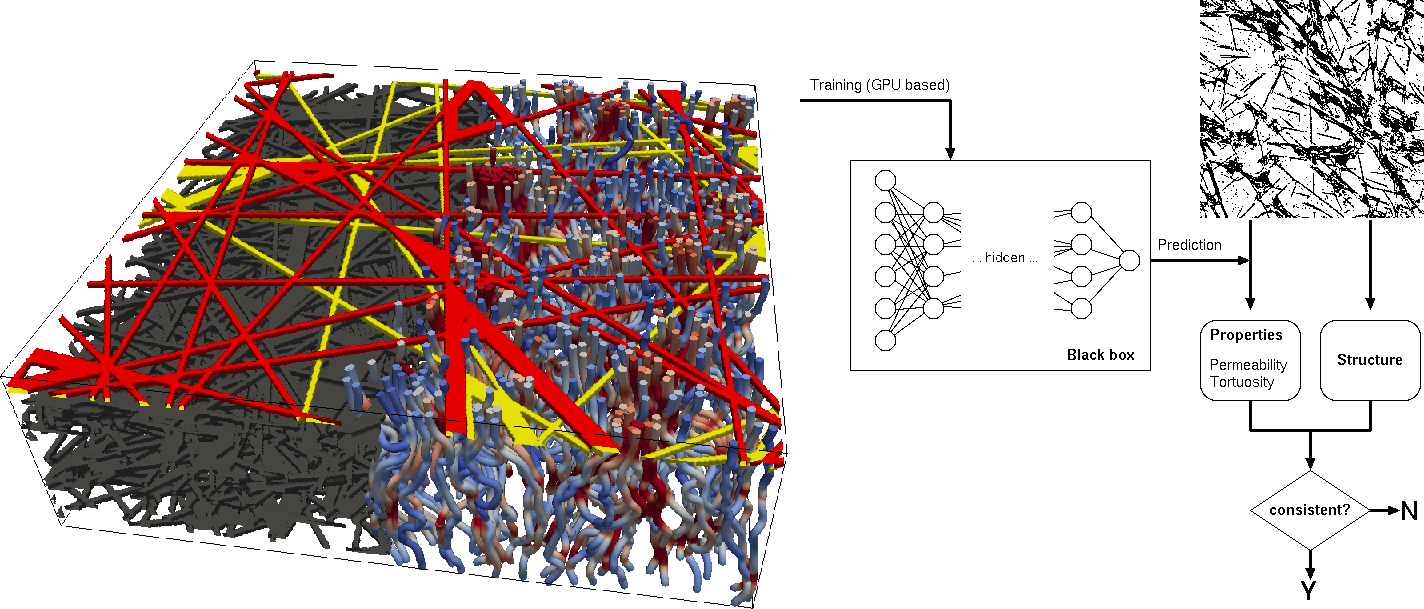
Gas diffusion layers (GDLs) are porous transport layers that are used in fuel cells to allow the transport of fluids from the flow channels to the membrane. This requires good gas permeability in the through-plane (TP) direction. For transport under the ribs of a flow field, a good permeability in the in-plane (IP) direction is also desired. Ye et al. [1] investigated the effect of GDL compression on the bypass of gases below the ribs of the flow field. A critical review of mesoscale modeling in electrochemical devices was presented by Ryan and Mukherjee [2]. Holzer et al. [3] evaluated the permeability of dry GDLs and several other properties of the micro-structure. The porosity and shape of the pores was investigated by Zenyuk et al. [4]. They used X-ray tomography for the analysis of structural properties of a GDL under compression. Meanwhile, Bao et al. [5] reconstructed fiber-based GDLs, calculated the impact of compression on the micro-structure by means of the finite element method (FEM), and then analyzed the compressed GDL using computational fluid dynamics (CFD). The relevance of compression on the properties of GDLs was shown by Bosomoiu et al. [6], who investigated the micro-structure of paper-type GDLs via X-ray tomography. They analyzed GDLs under ribs and under the channels of a flow field, and also analyzed them in fresh and aged states. Permeability and tortuosity were some of the features addressed in their studies. Mukherjee et al. [7] measured the TP and IP permeability of GDLs, with and without polytetrafluorethylene (PTFE), and with and without micro-porous layer (MPL). In order to reduce costs, GDLs from novel materials were developed by Leonard et al. [8]. Zhang et al. [9] analyzed GDL properties using Lattice–Boltzmann (LB) simulations based on reconstructed micro-structures. Artificial intelligence (AI) enters the picture when machine learning (ML) or the deep learning (DL) methods are applied in the field of electrochemical research. Ding et al. [10] recently presented an overview of the application of ML in the field of fuel cell research, in particular for polymer electrolyte fuel cells (PEFCs). However, the use of AI methods is still growing and is beyond of the scope of this extensive review article. In previous investigations, the suitability of convolutional neural networks (CNN) was demonstrated by Froning et al. [11] for the prediction of the TP permeability of paper-type GDLs. The data were previously generated via LB simulations. In a similar manner, a CNN was developed by Cawte and Bazylak [12], predicting the permeability of fibrous GDLs. In their study they used the pore network modeling (PNM) method to generate their data. The accuracy of predicting the permeabilities of porous media using CNNs in the context of LB simulations was shown by Wang et al. [13]. In turn, the relevance of investigations in the GDL micro-structure was pointed out by Pan et al. [14], who summarized the mechanics, techniques and modeling approaches for GDL degradation. Using similar ML methods, Jafarizadeh et al. [15] coupled their ML application with CFD and applied it to a variety of metal foams. Yeh et al. [16] presented a CNN in the field of signal processing that is robust against noise added to datasets for prediction. The performance prediction of PEFCs by a neural network (NN) was coupled to flow channel optimization by Li et al. [17]. Applied to X-ray tomography, Shum et al. [18] used ML algorithms for the water segmentation in GDLs of PEFCs. For high-temperature PEFCs, Zhu et al. utilized a NN to predict performance for a variety of parameters [19], achieving a percentage accuracy compared to numerical methods. Buchaniec et al. [20] investigated the accuracy of gray-box models and applied this technique to the triple-phase boundaries (TPBs) in the micro-structure of a solid oxide fuel cell (SOFC) anode. Meanwhile, Yasuda et al. [21] presented a data-driven framework for the characterization of porous materials, coupling ML methods with genetic algorithms. The permeability was in the focus of their recent studies. In the field of geoscience, ML and DL methods are well established. Arigbe et al. [22] used DL for the prediction of relative permeability in real-time. However, there are also pitfalls in the use of AI. As reported by Hurtz [23], an AI program that declassified world-class Go players was recently defeated by an amateur Go player, underlining the fact that any AI code is bounded by the scope of its training data.
Previous work [11] was extended in order to apply its previously-developed CNN to real image data. Although the training and classical validation was performed on artificial data, real data from image sources can suffer from image errors, which are caused by several factors. In Section 2, methods, both AI-related and physics-based, are briefly summarized. Furthermore, several groups of image data are introduced. The preparation of the data for the training process and the subsequent prediction is described in Section 3. The validation in Section 4 addresses not only the validation of the artificial geometry data but also aspects that occurred in real data obtained from image sources. The results are presented in Section 5. After discussing them in Section 6, the work is summarized in Section 7.
2. Methods and Data
Fibrous GDLs of the Toray type are characterized with the ML method, in particular using a CNN presented by Froning et al. [11], as shown in Section 2.1 and Section 2.2. The image data of the micro-structure is labeled by post-processing LB simulations, as is briefly described in Section 2.3. Subsequently, Section 2.4 and Section 2.5 provide an overview on the data in the study. Finally, Section 2.6 introduces the physical interpretation of the results predicted by the CNN.
2.1. An Overview on the Machine Learning Model
As outlined in Section 2.2, a CNN was developed in order to predict characteristics of porous structures, namely the permeability and tortuosity. The geometry of the structures is specified using black/white (BW) images. The CNN was trained using the same micro-structures as published earlier [24]. Each data point was data point was given by 65 images, having dimensions of 512x512. The resolution of them was . The Section 2.4 summarizes the details.
Finally, the ML model was applied to real micro-structures introduced in Section 2.5. This data has different sizes and image resolutions than the training data. Furthermore, imaging errors are present that were not contained in the training data.
The high performance computer CLAIX at RWTH Aachen University was used for the training phase. Each of the graphic nodes of this system has two graphics processing units (GPUs) of the kind ‘Tesla V100 SXM2 32 GB’.
2.2. Convolutional Neural Network Model
The Python-based framework TensorFlow [25] was used to implement a CNN for the prediction of the characteristics of a GDL with its fiber-based micro-structure. Its architecture, as in previous work [11], is illustrated in Figure 1. The red-shaped layers are also analyzed in detail. The first layer, marked as ‘0/Input’, contains the input micro-structure of 512x512x65 dimensions. The parameters of the convolution layers were chosen to reduce the flat shape of the 3D filters to a more regular one, from 512x512x65 on the input layer, down to, e.g., 8x8x8 in the eighth layer. Layer ‘1/Convolution’ is the first hidden layer of the CNN. The structure shrank in both the x and y directions. The layer ‘3/Convolution’ also shrank in two dimensions. The third dimension was not reduced because of its flat 3D shape. The architecture shown in Figure 1 was already used earlier [11] to predict the TP permeability of Toray GDL. The same architecture – predicting one feature out of a stack of images – was trained separately to four features, namely TP permeability, TP tortuosity, IP permeability, and IP tortuosity. All of these the features were simulated earlier by means of the LB method [24].
2.3. Lattice–Boltzmann Simulations
Material characteristics have been previously obtained from fiber-based GDLs using the technique of LB simulations [24,26,27]. The micro-structure of a porous GDL is specified by a stack of BW images. Using a stochastic geometry model, several representations of a paper-type GDL were constructed, being analyzed by Froning et al. [24,26]. This work employs this method to obtain the permeability and tortuosity of Toray GDL given by a stack of images, both TP and IP. Because of the layer-wise construction of the fibers in the plane, the IP characteristics only needed to be determined for one direction. Another kind of GDL, represented by a stochastic model and also as a reconstruction of real data, was investigated by Froning et al. [27].
Transport simulations of gas flow through the porous micro-structure were calculated in a domain defined by a series of BW images. A small free space buffer was added upstream and downstream of the porous media to allow for physically meaningful boundary conditions. As was described in more detail in Froning et al. [24], a velocity boundary was applied at the input and a constant pressure condition at the output. Wall boundary conditions were specified at the other four sides of the simulation domain. As before, the permeability was calculated from the resulting flow field using Darcy’s law.
In Equation (1) the permeability is a function of the flux q, the dynamic viscosity , and the pressure drop . The tortuosity was calculated by Equation (2).
This is the simplest variant of a set of equations presented by Koponen et al. [28] for the estimation of the flow-based tortuosity in porous structures. The tortuosity was calculated as the ratio between the average values of the absolute velocity and of the x component. The transport simulations were run on JURECA [29].
2.4. Basic Data
The training data for the ML model is referred to as basic data in this section. Each data point consists of a stack of images constructed by a geometry model developed by Thiedmann et al. [30] and Wang et al. [31]. They developed a fiber model of the micro-structure of Toray 090 GDL. Their studies are based on the stochastic analysis of real fibers. In order to achieve the porosity of the real material they added binder material, again using a stochastic approach. The binder model of Thiedmann et al. [30] is represented by a width of binder covering parts of the fibers [30]. Figure 2 illustrates the this approach in selected images.
The data in Figure 2A—D were published by Froning et al. [24], both uncompressed and compressed. The total number of available data points is given by
- the number of the realizations of the fiber geometry: 25,
- the number of parameters used for different binder distributions: four,
- and the number of compression levels - six steps from 0% (uncompressed) to 50% – in steps of 10% – were used.
In this way, a total number of geometries could be available. It was already stated by Froning et al. [24] that not all of the LB simulations did converge. This was especially the case for the higher compressed micro-structures. From this reason, only 541 data points were available for training.
Based on Thiedmann et al. [30], the underlying fibers were also the subject of a high-accuracy LB simulation by Lintermann and Schröder [32]. They used periodic boundary conditions and a circular cross section of the fibers, whereas in this work wall boundary conditions were used, with coarser mesh based on a quadratic cross-section of the fibers. The reason was to obtain a better comparison with real data from X-ray tomography [30,31].
2.5. Real Data
The ML model was applied to real data from different sources.
- R1
- One image series of Toray GDL was reconstructed from the BESSY synchrotron, the image source from which the GDL model of Thiedmann et al. [30] was validated.
- R2
- Two image series were obtained from a Nano CT Zeiss Xradia Versa 420 at the IEK-14 at the Forschungszentrum Jülich, allowing a minimal voxel size of . Hoppe [33] investigated Toray TGP-H-060 GDL, one series with labels (Figure 5), and
- R3
- one without (Figure 6).
In 2011, series R1 was obtained from the BESSY synchrotron for validation of the Thiedmann geometry model [30]. The gray level images were segmented into binary BW images, but their quality was not sufficient for LB simulations. Figure 3 shows two of the 200 images of dimensions 1250x1250. The images have a resolution of . That defines a square section with a side length of 1.875 mm. The porosity of the image stack – calculated by counting pixels – is 0.782.
The resolution of the images in Figure 3 is the same as in the training data, but the images are larger and are more than 130. This led to the opportunity to randomly select a number of 3D sections of dimensions 130x512x512 out of the image stack of 200x1250x1250. The resulting permeabilities (TP and IP) predicted by the CNN show a statistical variation, changing with the position of the 3D subset.
The difference between Toray 060 and 090 is only the thickness: according to the data sheet, Toray 060 has a thickness of , whereas Toray 090 has one of . Hoppe [33] experimnentally analyzed the micro-structure of GDLs of different types, one of them being Toray GDL under compression. Figure 4 (A) displays schematically the membrane electrode assembly (MEA) with a GDL on both sides in the experimental setup of a compression device. The images of the R2 and R3 series were obtained from a Nano CT Zeiss Xradia Versa 420. Figure 4 (B) shows an example.
GDLs were compressed by different levels of compression. Series R2 was from the channel side of a punch with a 1.0 mm slit, representing the 1.0 mm channel of a flow field. Series R3 was from the block side, i.e., the flat punch vis-à-vis a punch with a 0.8 mm slit. The images of both the R2 and R3 series spanned a region from one rib across the channel to the other rib in the scheme of Figure 4A. Hoppe [33] observed that the entire MEA deformed under compression, and therefore affected both GDLs. The GDL on the channel side also intruded into the channel.
The gray level images were segmented to black/white (BW) ones in order to provide binary micro-structures for the LB simulations as introduced by Froning et al. [24]. The BW images in Figure 5 and Figure 6 display similar segmentation artifacts as those from the X-ray synchrotron in Figure 3. BW images of series R2 and R3 could only be created in thin slices – no more than 40 images per sample – due to the low quality of the images. Because this is too small for robust LB simulations [24], the image packs were stacked one above each other until at least 120 images were achieved. Regarding the transport simulations, an unrealistic periodicity was introduced into the micro-structure. Care must be taken at these inner breaking faces, as they can possibly cause unpredictable side effects. The dimensions of the image series are summarized in Table 1.
2.6. Evaluation of the Predictions
In particular, the predictions of the real data from Section 2.5 are interpreted according to established relationships known in the characterization of porous material.
Based on the work of Tomadakis and Robertson [34], the Kozeny–Carman trend was already successfully used by Froning et al. [24] in the description of porous material.
With the Kozeny–Carman Equation (3), the permeability of a porous material is related to morphological characteristics of the micro-structure, namely the total volume and the inner surface of the solid structure . is the Kozeny constant, representing the shape of the micro-structure. Furthermore, it is known that the product of the permeability and tortuosity is related to the fraction of the total volume and the inner surface
– as long as the shape of the micro-structure does not change under compression. That allows a Kozeny–Carman (KC) trend to be defined.
The subscript ‘’ in Equation (5) denotes a reference value of compression. In [24], a value of 0% was used. With this relationship, the consistency of , calculated for compressed material (), can be justified. The training data (from [24]) consists of ensembles of 25 stochastic micro-structures for each pair of binder type and compression level. When the Kozeny–Carman trend (equation (5)) was applied to the LB simulations, the trend was applied with ‘’ being the average values of 25 realizations of compression for each binder type.
3. Data Preparation
3.1. Domain Size Normalization
The training data from previous investigations [24] were also used in this study. The micro-structures are represented by series of images of the dimensions 512x512 each. The number of images is related to the amount of compression. They are ranging from 65 in case of 50% compression up to 130 for uncompressed micro-structures. Because a fixed size is needed for the CNN, the data must be transformed to this domain size. Based on the given data, the target size was chosen to be 65x512x512. For each fiber layer, the geometry model defines five BW images in the uncompressed state [24], all of them being identical. Compressing the images from 130 to 65 creates gray level images in which intermediate gray levels where different images are merged by the compression routine. Figure 7 illustrates intermediate gray levels on image triples after compression, exemplarily on two image series. The labels in Figure 7 and Figure 2 – (B) and (D) – are corresponding to each other.
3.2. Real Data
The image stack R1 has images larger than those of the training dataset. The image resolution of both the training data and the R1 series is the same: . For the prediction, 50 sections of dimensions 130x512x512 at random positions were cut out of the images stack of 200x1250x1250. Random positions were chosen to avoid any systematic influence. As a consequence, a set of 50 geometries were available for the prediction.
The real data of series R2 and R3 introduced in Section 2.5 has images with a resolution of , whereas the CNN was trained with image resolutions of . In a first step, the images were re-scaled – a correction step in the x and y directions, which was easily done with the tools of ImageMagick [35]. In the z-direction, this re-scaling must be overlaid with the compression algorithm introduced in Section 3.1. The R2 series has images larger than 512x512. For the prediction, a section of 512x512 was cut out of each of the R2 images. The images of R3 are smaller than 512 pixels in y direction, even after re-scaling. The images are first doubled, introducing a break in the center of the images, and then a 512x512 section was cut out, like in R2.
4. Validation
As in previous work [11], the data was validated using five-fold cross-validation. Fold no. 4 was selected for presenting detailed results.
The CNN was trained using 244 iterations with different labels, all of them from fold no. 4:
- A)
- permeability
- B)
- tortuosity
- C)
- permeability
- D)
- tortuosity
It was necessary to train the tortuosity features with instead of . Five folds were trained, each of them randomly splitting the data into training and test data in the ratio of 80:20. The development of the MSE during the training of fold no. 4 is displayed in Figure 8.
The training history does not appear suspicious, but an overfitting effect was observed in the IP tortuosity of the real material, series R3, where was predicted. The training was re-run with only 122 iterations, and was then used for the prediction of results. This is also discussed in detail in Section 5.
The three layers that were marked in red shapes in Figure 1 are visualized in Figure 9, as suggested by Nguyen et al. [36]. The data in each layer is three-dimensional. For visualization, only the first image of the image stack is shown. Figure 9 displays the first image of the input data. Convolution layers, together with succeeding filters, help to detect features of the input data. Typically, on top of the network, local features are detected, whereas deeper in the network, more complex features are learned [37]. The convolution creates smaller image stacks but several channels, eight in the case of the layer ‘1/Convolution’ and 16 in the case of the layer ‘3/Convolution’. In the diagram, only four of each are displayed. The subsequent layers show the result of the convolution steps that creates gray level images, although the visualization in Figure 9 displays different colors. The gray level images become blurred as the size is reduced. The hidden layers of the CNN represent parameters of the fitting procedure during the training. In the prediction, they show a kind of shadow of the input data. With increasing depth in the network, the shadows become increasingly blurred, mimicking more complex features of the micro-structure.
5. Results
The CNN was trained separately with permeability and tortuosity to achieve models to predict permeability and tortuosity. A training with was not successful, which demonstrates the dependency of the method from the absolute range of the characteristics. The accuracy of the predicted permeability and tortuosity is shown in Figure 10. The diagrams contain the values of the uncompressed data of fold no. 4. The predictions were obtained using separated CNN weights for permeability and tortuosity, TP and IP.
The symbols in Figure 10a–c are close to the ideal line, representing a good agreement between the predicted data and labeled data. The effect of the binder type on the permeability and TP tortuosity, which was not explicitly trained, is represented by the predicted values – the information is inherent in the trained data. The scale of Figure 10d is different from Figure 10b, because the IP tortuosity varies in a closer range than the TP tortuosity. This is in agreement with the original data calculated by LB simulations by Froning et al. [24].
The real data of Toray GDL consists of 50 sub-regions randomly cut out of the image stack of series R1, and two series R2 and R3 taken from an channel/rib assembly. The predicted data for the cut-outs of series R1 are summarized in Table 2. The product of the permeability and tortuosity will be used later in this section in comparison with series R2 and R3.
In Table 2, the min/max values of the product are different from the product of the separate min/max values of and , because low values for the tortuosity typically correspond to high values for the permeability and vice versa. The average values in Table 2 are close to the medians for all features. This confirms the absence of skewness in the distributions that could occur in the systematic selection of the positions from where the sub-sections were cut out of the R1 image stack. The average values of the predicted TP and IP permeabilities and tortuosities are compared with the previously-published [24] values, separated according to the inherent binder model as introduced in Figure 2. The predicted values best fit to the published values of binder models B and C, representing binder widths of and . The statistical spread can be expressed by the dimensionless variation coefficient , being the standard deviation and the average value. The variation coefficient of the permeability (TP and IP) is smaller than that of the training data as published in [24]. The variation coefficient of the predicted tortuosities is close to that of the predicted permeabilities. Within the training data, it was somewhat smaller.
The binder widths in variants A and D were extreme values in the original development of the underlying binder model by Thiedmann et al. [38]. Manual measurements of the binder width in the BW images as shown in Figure 3 are hardly representative because of significant imaging errors. These imaging errors also inhibited a successful LB simulation of this micro-structure.
In series R2, the GDL was embedded in an assembly with a 1.0 mm channel width and a 0.8 mm channel width in series R3. The resolution of the images – – was adapted to the resolution of the training data in the pre-processing step (). Table 3 summarizes the predicted permeability.
The LB simulations in the IP direction did not converge on meaningful physical values. It is believed that the tight stacking of the images led to significant errors at the artificial inner breaking faces. These breaking faces are closer than the minimum domain size (100 in each coordinate direction) for these kinds of LB simulations, as identified by Froning et al. [24].
The inner structure is characterized by the porosity and the relationship which is used in the Kozeny–Carman trend, Equations (4) and (5). The values for in the table are related to the resolution of of the original images (see Section 3.2).
Mangal et al. [39] measured the TP permeability of Toray GDL as , which is closer to the results of the LB simulations in artificial structures by Froning et al. [24] than to those from the segmentations of real data in Table 3. This indicates that the image segmentation possibly caused larger errors than the LB ones and the ML predictions.
The IP permeability is systematically larger than the TP permeability, which is consistent with systematic investigations into the artificial micro-structures of Toray GDLs [24]. The permeability of series R2 along the compression of the material is depicted in Figure 11. Series R3 is shown in Figure 12.
Feser et al. [40] measured the IP permeability of three kinds of GDL, one of them being Toray 060, under mechanical compression. They observed a decrease in the IP permeability of Toray GDL by a factor of approximately two under compressions of up to 24%. Their experiments showed variances of only 10–15%. This behavior is consistent with the predicted values in the IP columns of Table 3 and the corresponding symbols in Figure 11 and Figure 12.
The IP permeability and tortuosity were calculated in only one direction – the x coordinate – because the geometry model of Thiedmann et al. [30] was stochastically-invariant in the plane. The real data from Hoppe [33], however, was not invariant in its two IP directions because of the morphological changes of the micro-structure under compression. The x coordinate is the transport direction in the IP simulations. According to Figure 4, this direction is across the channel in the mechanical compression setup of Hoppe [33]. This fact may affect the LB simulations presented in Table 3 and Figure 11.
The consistency of the predicted data was evaluated via the product . According to Equation (4), a constant was fitted to match with . The latter characterizes the compression of the material, assuming an almost similar shape of the inner structure. Series R3 shows some outliers of in Table 3, namely for compression levels 24%, 28% and 31%.
The KC trend (Equation (4)) was fitted to the predicted values for for the real data from series R2 and R3. According to Equation (4), a constant factor was determined that minimized the sum of the squared errors. The resulting factor was 0.91 for the TP values and 1.77 for the IP ones. The relationship of series R2 is shown in Figure 13. The data is presented in relation to the compression. Therefore the straight line from the fit procedure follows the irregular shape of the displayed abscissa . The predicted values for show a good agreement with the Karman-Cozeny trend (equation(4)). Although the LB simulations in the IP direction failed in most cases, the ML predictions are also consistent in this case. The failing LB simulations may be a consequence of the fact that the images needed to be stacked upon each other. In IP direction, the wrong shear layers potentially led to a different type of error than in the TP direction. For comparison, the average of the predicted of the R1 series was also inserted in Figure 13, including a small error bar representing the standard deviation from Table 2. This entry for uncompressed data does not conflict with an extrapolation of the R2 series of compressed geometries in Figure 13.
The relationship of series R3 is shown in Figure 14. The fitted factors for the KC trend of this data were 0.65 for the TP direction and 1.32 for the IP one. In comparison to Figure 13, the predicted for the R3 series shows less agreement with than before, especially for higher compression levels. This is in accordance with the presence of outliers in the entries in Table 3. Also, the R1 value for is further away from a meaningful extrapolation of the corresponding values of the compressed R3 series in Figure 14 than it was previously, in the R2 series. The sub-optimal agreement of the KC trend with along the compression indicates that the underlying micro-structure – in this case its representation by BW images – changes its shape under compression.
The deviation in the KC trend in Figure 14 is in agreement with the observation that the LB simulations of these micro-structures failed more often than for the R2 series.
6. Discussion
The prediction of the permeability and tortuosity of Toray GDL was successfully applied to segmented images of the micro-structure of real data. A re-scale of different image resolutions and domain sizes led to consistent results.
Applied to real image data with unknown errors in the segmentation, overfitting effects were observed. In contrast to introductory examples [25], where the test dataset is usually of the same image quality as the training dataset, overfitting was not detected in the test data. Additional consistency checks were necessary in the case of the R3 series, where meaningless values () were predicted for the IP tortuosity.
As in previous work [24], the Kozeny–Carman trend on the product of both the permeability and tortuosity characteristics was applied to judge the consistency of the predicted results.
Using real data, re-sizing and re-scaling was applied to the micro-structure, because the CNN requires a 3D input geometry of fixed size. For this purpose, two image series, R2 and R3, were available.
The re-scaling from of the micro-structure to of the training data obviously did not hurt the accuracy: the features of the R2 series were satisfactorily predicted. That was not the case with the R3 series though.
One difference between the R2 and R3 series is the small size of the sample in the y direction. The images of both series must be stacked upon each other in direction z to achieve the the training size. Only for the R3 series was this procedure applied also in direction y. The inaccuracy of the R3 series was observed in both the TP and IP directions. Moreover, the images of R2 were taken from the channel side of the compression device setup. The R3 images were taken from the block side. Although it was observed by Hoppe [33] that the complete MEA was deformed under the channel, the impact of deformation on the GDL micro-structure is expected to be lower on the block side than on the channel one. The high relevance of the GDL deformation under compressed flow fields was shown by Hoppe et al. [41], who investigated the GDL compression under misaligned flow fields.
The IP characteristics of the training data were only available for one direction [24]. This is absolutely sufficient, given of the stochastic nature of the underlying geometry model [30]. The geometries of the training data were homogeneously compressed. In contrast, the real data of the R2 and R3 series were in-homogeneously compressed [33]: according to Figure 4, there are regions under the channel and under the rib. In the arrangement of Figure 4, the IP characteristics differ, along and perpendicular, to the channel. However, this cannot be distinguished by a model that was trained for homogeneous compression.
From the application’s view, the permeability of the GDL on the flow field side – R2 – is expected to be higher than that of the GDL on the block side – R3. This is indeed predicted by the ML model, but it must be conceded that the predictions of the R3 series possibly cannot be trusted because of the KC trend.
Nevertheless, it must be noted that imaging errors could have occurred in different degrees of severity in both series. In this work, the KC trend was used to justify the consistency of the ML predictions. It may be that other methods are viable for evaluating the accuracy of predictions in case an application were to suffer from other effects than the training data.
7. Conclusions
The CNN architecture for the prediction of permeability developed in previous work is also able to train and predict the tortuosity of paper-type GDLs. Applied to images from a different source than those of the training set, the consistency of the prediction must be verified by an additional criterion. The effect of compression on the characteristics of the porous media was verified using the Kozeny-Carman trend. This relationship was also used to identify the sub-optimal segmentation of the micro-structure, leading to a deviation between the Kozeny–Carman equation and the product of the permeability and tortuosity. For different situations, another criterion could possibly help justify the consistency of the predictions.
Author Contributions
Conceptualization, D.F. and E.H.; Formal analysis and methodology, D.F.; Investigation, D.F. and E.H.; Software, D.F.; Validation, D.F. and E.H.; Writing, D.F.; Supervision, R.P.
Funding
This research was funded by the Deutsche Forschungsgemeinschaft (DFG, German Research Foundation) – 491111487.
Data Availability Statement
Not applicable
Acknowledgments
The authors gratefully acknowledge the computing time provided to them at the NHR Center NHR4CES at RWTH Aachen University (project number p0020317), which is funded by the Federal Ministry of Education and Research, and the state governments participating on the basis of the resolutions of the GWK for national high performance computing at universities (www.nhr-verein.de/unsere-partner). The authors acknowledge the computing time granted by the JARA Vergabegremium and provided on the JARA Partition part of the supercomputer JURECA at Forschungszentrum Jülich.
Conflicts of Interest
The authors declare no conflict of interest.
References
- Ye, D.H.; Gauthier, E.; Cheah, M.J.; Benziger, J.; Pan, M. The Effect of Gas Diffusion Layer Compression on Gas Bypass and Water Slug Motion in Parallel Gas Flow Channels. AIChE J. 2015, 61, 355–367. [Google Scholar] [CrossRef]
- Ryan, E.M.; Mukherjee, P.P. Mesoscale modeling in electrochemical devices—A critical perspective. Prog. Energy Combust. Sci. 2019, 71, 118–142. [Google Scholar] [CrossRef]
- Holzer, L.; Pecho, O.; Schumacher, J.; Marmet, P.; Stenzel, O.; Büchi, F.; Lamibrac, A.; Münch, B. Microstructure-property relationships in a gas diffusion layer (GDL) for Polymer Electrolyte Fuel Cells, Part I: Effect of compression and anisotropy of dry GDL. Electrochim. Acta 2017, 227, 419–434. [Google Scholar] [CrossRef]
- Zenyuk, I.V.; Parkinson, D.Y.; Connolly, L.G.; Weber, A.Z. Gas-diffusion-layer structural properties under compression via X-ray tomography. J. Power Sources 2016, 328, 364–376. [Google Scholar] [CrossRef]
- Bao, Z.; Li, Y.; Zhou, X.; Gao, F.; Du, Q.; Jiao, K. Transport properties of gas diffusion layer of proton exchange membrane fuel cells: Effects of compression. Int. J. Heat Mass Transf. 2021, 178, 121608. [Google Scholar] [CrossRef]
- Bosomoiu, M.; Tsotridis, G.; Bednarek, T. Study of effective transport properties of fresh and aged gas diffusion layers. J. Power Sources 2015, 285, 568–579. [Google Scholar] [CrossRef]
- Mukherjee, M.; Bonnet, C.; Lapique, F. Estimation of through-plane and in-plane gas permeability across gas diffusion layers (GDLs): Comparison with equivalent permeability in bipolar plates and relation to fuel cell performance. Int. J. Hydrog. Energy 2020, 45, 13428–13440. [Google Scholar] [CrossRef]
- Leonard, D.; Babu, S.K.; Baxter, J.; III, H.M.; Cullen, D.; Borup, R. Natural fiber-derived gas diffusion layers for high performance, lower cost PEM fuel cells. J. Power Sources 2023, 564, 232619. [Google Scholar] [CrossRef]
- Zhang, H.; Zhu, L.; Harandi, H.B.; Duan, K.; Zeis, R.; Sui, P.C.; Chuang, P.Y.A. Microstructure reconstruction of the gas diffusion layer and analyses of the anisotropic transport properties. Energy Convers. Manage. 2021, 241, 114293. [Google Scholar] [CrossRef]
- Ding, R.; Zhang, S.; Chen, Y.; Rui, Z.; Hua, K.; Wu, Y.; Li, X.; Duan, X.; Wang, X.; Li, J.; Liu, J. Application of Machine Learning in Optimizing Proton Exchange Membrane Fuel Cells: A Review. Energy AI 2022, 9, 100170. [Google Scholar] [CrossRef]
- Froning, D.; Wirtz, J.; Hoppe, E.; Lehnert, W. Flow Characteristics of Fibrous Gas Diffusion Layers Using Machine Learning Methods. Appl. Sci. 2022, 12, 12193. [Google Scholar] [CrossRef]
- Cawte, T.; Bazylak, A. A 3D convolutional neural network accurately predicts the permeability of gas diffusion layer materials directly from image data. Curr. Opin. Electrochem. 2022, 35, 101101. [Google Scholar] [CrossRef]
- Wang, Y.D.; Chung, T.; Armstrong, R.T.; Mostaghimi, P. ML-LBM: Predicting and Accelerating Steady State Flow Simulation in Porous Media with Convolutional Neural Networks. Transp. Porous Media 2021, 138, 49–75. [Google Scholar] [CrossRef]
- Pan, Y.; Wang, H.; Brandon, N.P. Gas diffusion layer degradation in proton exchange membrane fuel cells: Mechanisms, characterization techniques and modelling approaches. J. Power Sources 2021, 513, 230560. [Google Scholar] [CrossRef]
- Jafarizadeh, A.; Ahmadzadeh, M.; Mahmoudzadeh, S.; Panjepour, M. A New Approach for Predicting the Pressure Drop in Various Types of Metal Foams Using a Combination of CFD and Machine Learning Regression Models. Transp. Porous Media 2023, 147, 59–91. [Google Scholar] [CrossRef]
- Yeh, R.; Hasegawa-Johnson, M.; Do, M.N. Stable and symmetric filter convolutional neural network. 2016 IEEE International Conference on Acoustics, Speech and Signal Processing (ICASSP). IEEE, 2016, pp. 2652–2656. [CrossRef]
- Li, H.W.; Liu, J.N.; Yang, Y.; Lu, G.L.; Qiao, B.X. Coupling flow channel optimization and Bagging neural network to achieve performance prediction for proton exchange membrane fuel cells with varying imitated water-drop block channel. Int. J. Hydrog. Energy 2022, 47, 39987–40007. [Google Scholar] [CrossRef]
- Shum, A.D.; Liu, C.P.; Lim, W.H.; Parkinson, D.Y.; Zenyuk, I.V. Using Machine Learning Algorithms for Water Segmentation in Gas Diffusion Layers of Polymer Electrolyte Fuel Cells. Transp. Porous Med. 2022, 144, 715–737. [Google Scholar] [CrossRef]
- Zhu, G.; Chen, W.; Lu, S.; Chen, X. Parameter study of high-temperature proton exchange membrane fuel cell using data-driven models. Int. J. Hydrog. Energy 2019, 44, 28958–28967. [Google Scholar] [CrossRef]
- Buchaniec, S.; Gnatowski, M.; Brus, G. Integration of Classical Mathematical Modeling with an Artificial Neural Network for the Problems with Limited Dataset. Energies 2021, 14, 5127. [Google Scholar] [CrossRef]
- Yasuda, T.; Ookawara, S.; Yoshikawa, S.; Matsumoto, H. Materials processing model-driven discovery framework for porous materials using machine learning and genetic algorithm: A focus on optimization of permeability and filtration efficiency. Chem. Eng. J. 2023, 453, 139540. [Google Scholar] [CrossRef]
- Arigbe, O.D.; Oyeneyin, M.B.; Arana, I.; Ghazi, M.D. Real-time relative permeability prediction using deep learning. J. Petrol. Explor. Prod. Technol. 2018, 9, 1271–1284. [Google Scholar] [CrossRef]
- Hurtz, S. Brettspiel Go: Hobbyspieler schlägt "übermenschliche" KI. https://www.sueddeutsche.de/wirtschaft/go-ki-kellin-pelrine-lee-sedol-alphago-hobbyspieler-1.5754972. Online: 2023-02-20 20:12.
- Froning, D.; Brinkmann, J.; Reimer, U.; Schmidt, V.; Lehnert, W.; Stolten, D. 3D analysis, modeling and simulation of transport processes in compressed fibrous microstructures, using the Lattice Boltzmann method. Electrochim. Acta 2013, 110, 325–334. [Google Scholar] [CrossRef]
- Galeone, P. Hands-On Neural Networks with TensorFlow 2.0; Packt Publishing: Birmingham, UK, 2019. [Google Scholar]
- Froning, D.; Gaiselmann, G.; Reimer, U.; Brinkmann, J.; Schmidt, V.; Lehnert, W. Stochastic Aspects of Mass Transport in Gas Diffusion Layers. Transp. Porous Media 2014, 103, 469–495. [Google Scholar] [CrossRef]
- Froning, D.; Yu, J.; Gaiselmann, G.; Reimer, U.; Manke, I.; Schmidt, V.; Lehnert, W. Impact of compression on gas transport in non-woven gas diffusion layers of high temperature polymer electrolyte fuel cells. J. Power Sources 2016, 318, 26–34. [Google Scholar] [CrossRef]
- Koponen, A.; Kataja, M.; Timonen, J. Tortuous flow in porous media. Phys. Rev. E 1996, 54, 406–410. [Google Scholar] [CrossRef] [PubMed]
- Krause, D.; Thörnig, P. JURECA: Modular supercomputer at Jülich Supercomputing Centre. J. Large-Scale Res. Facil. JLSRF 2018, 4. [Google Scholar] [CrossRef]
- Thiedmann, R.; Fleischer, F.; Hartnig, C.; Lehnert, W.; Schmidt, V. Stochastic 3D Modeling of the GDL Structure in PEMFCs Based on Thin Section Detection. J. Electrochem. Soc. 2008, 155, B391–B399. [Google Scholar] [CrossRef]
- Wang, Y.; Cho, S.; Thiedmann, R.; Schmidt, V.; Lehnert, W.; Feng, X. Stochastic modeling and direct simulation of the diffusion media for polymer electrolyte fuel cells. Int. J. Heat Mass Transf. 2010, 53, 1128–1138. [Google Scholar] [CrossRef]
- Lintermann, A.; Schröder, W. Lattice–Boltzmann simulations for complex geometries on high-performance computers. CEAS Aeronaut. J. 2020, 11, 745–766. [Google Scholar] [CrossRef]
- Hoppe, E. Kompressionseigenschaften der Gasdiffusionslage einer Hochtemperatur-Polymerelektrolyt-Brennstoffzelle. PhD thesis, RWTH Aachen University, 2021.
- Tomadakis, M.M.; Robertson, T.J. Viscous Permeability of Random Fiber Structures: Comparison of Electrical and Diffusional Estimates with Experimental and Analytical Results. J. Compos. Mater. 2005, 39, 163–188. [Google Scholar] [CrossRef]
- The ImageMagick Development Team. ImageMagick. https://imagemagick.org. Accessed: 2021-01-04.
- Nguyen, A.; Yosinski, J.; Clune, J. Understanding Neural Networks via Feature Visualization: A Survey. In Explainable AI: Interpreting, Explaining and Visualizing Deep Learning; Springer International Publishing, 2019; pp. 55–76. 76. [CrossRef]
- El-Amir, H.; Hamdy, M. Deep Learning Pipeline; Apress, Berkeley, CA, 2020. [CrossRef]
- Thiedmann, R.; Hartnig, C.; Manke, I.; Schmidt, V.; Lehnert, W. Local Structural Characteristics of Pore Space in GDLs of PEM Fuel Cells Based on Geometric 3D Graphs. J. Electrochem. Soc. 2009, 156, B1339. [Google Scholar] [CrossRef]
- Mangal, P.; Pant, L.M.; Carrigy, N.; Dumontier, M.; Zingan, V.; Mitra, S.; Secanell, M. Experimental study of mass transport in PEMFCs: Through plane permeability and molecular diffusivity in GDLs. Electrochim. Acta 2015, 167, 160–171. [Google Scholar] [CrossRef]
- Feser, J.; Prasad, A.; Advani, S. Experimental characterization of in-plane permeability of gas diffusion layers. J. Power Sources 2006, 162, 1226–1231. [Google Scholar] [CrossRef]
- Hoppe, E.; Janßen, H.; Müller, M.; Lehnert, W. The impact of flow field plate misalignment on the gas diffusion layer intrusion and performance of a high-temperature polymer electrolyte fuel cell. J. Power Sources 2021, 501, 230036. [Google Scholar] [CrossRef]
Figure 1.
CNN architecture of the proposed ML model.
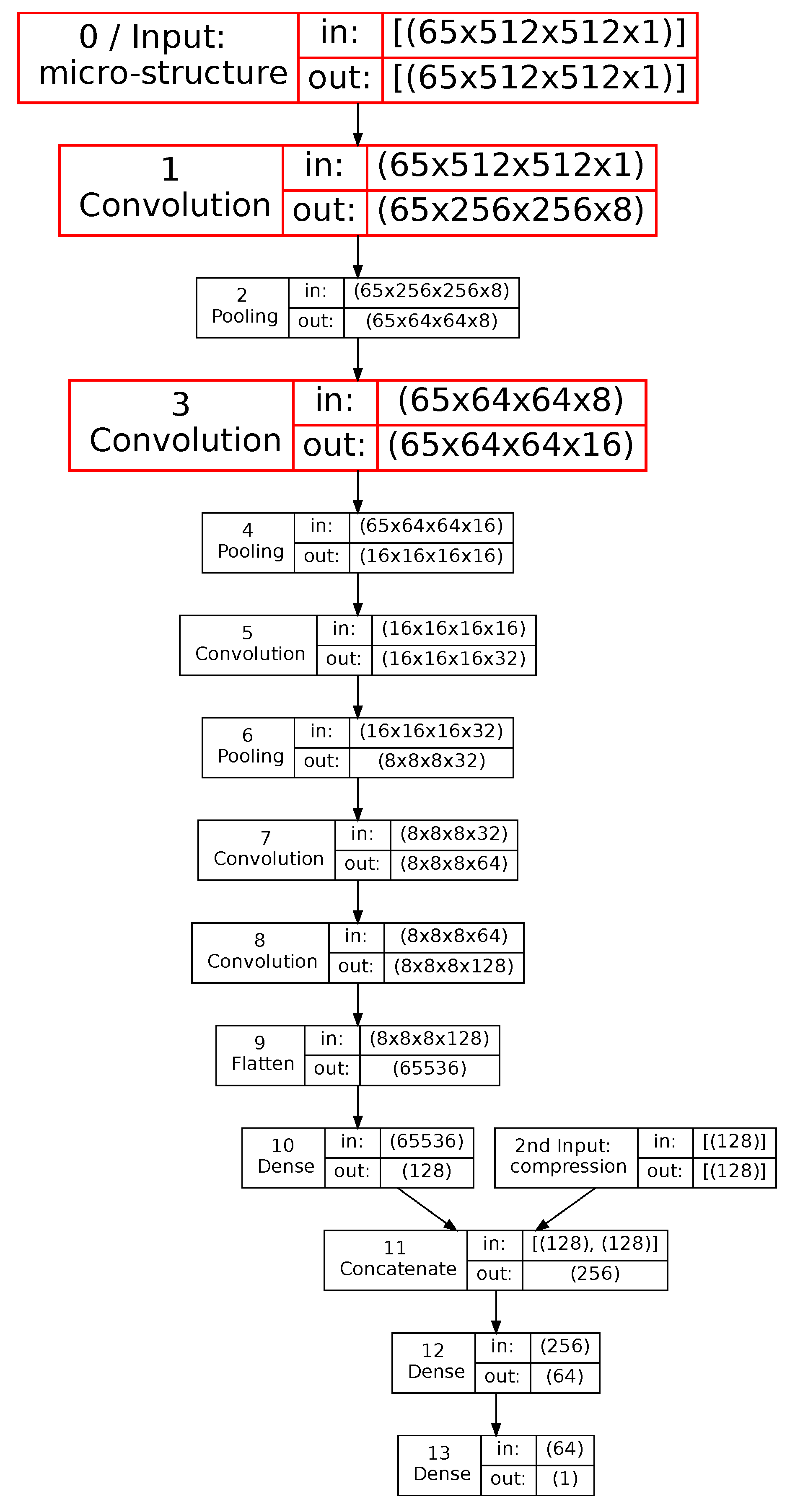
Figure 2.
Four different radii of binder illustrated on selected representations of fibers; A) = ; B) = ; C) = ; and D) .
Figure 2.
Four different radii of binder illustrated on selected representations of fibers; A) = ; B) = ; C) = ; and D) .
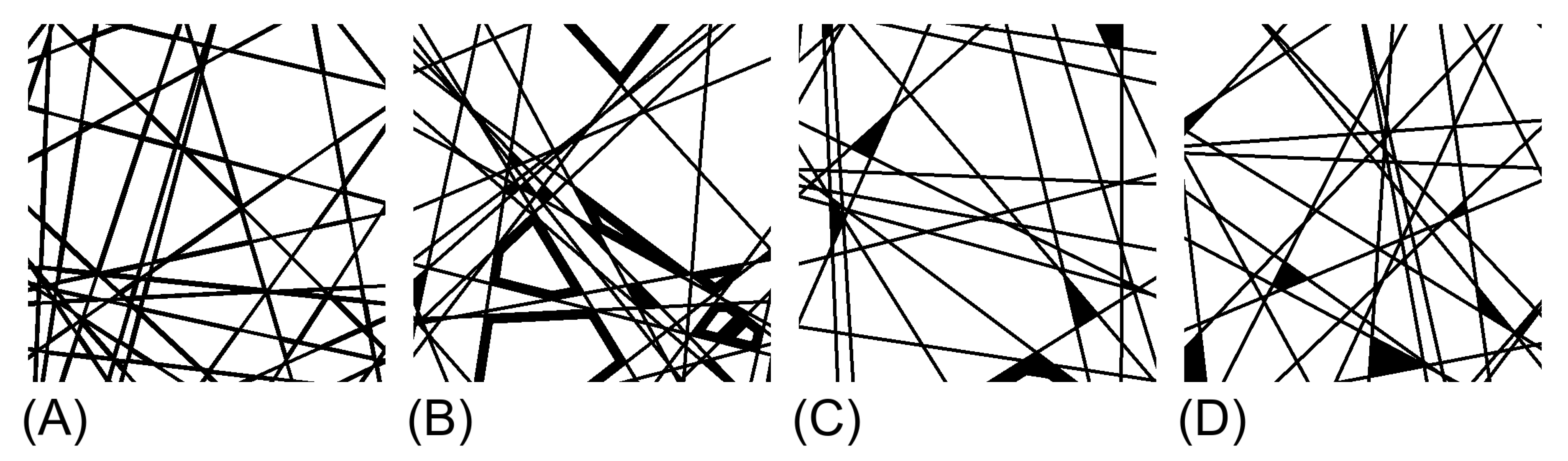
Figure 3.
X-ray synchrotron images of dimensions 1250x1250 from Toray 090 material; A) image no. 56 of 200; B) image no. 163 of 200.
Figure 3.
X-ray synchrotron images of dimensions 1250x1250 from Toray 090 material; A) image no. 56 of 200; B) image no. 163 of 200.
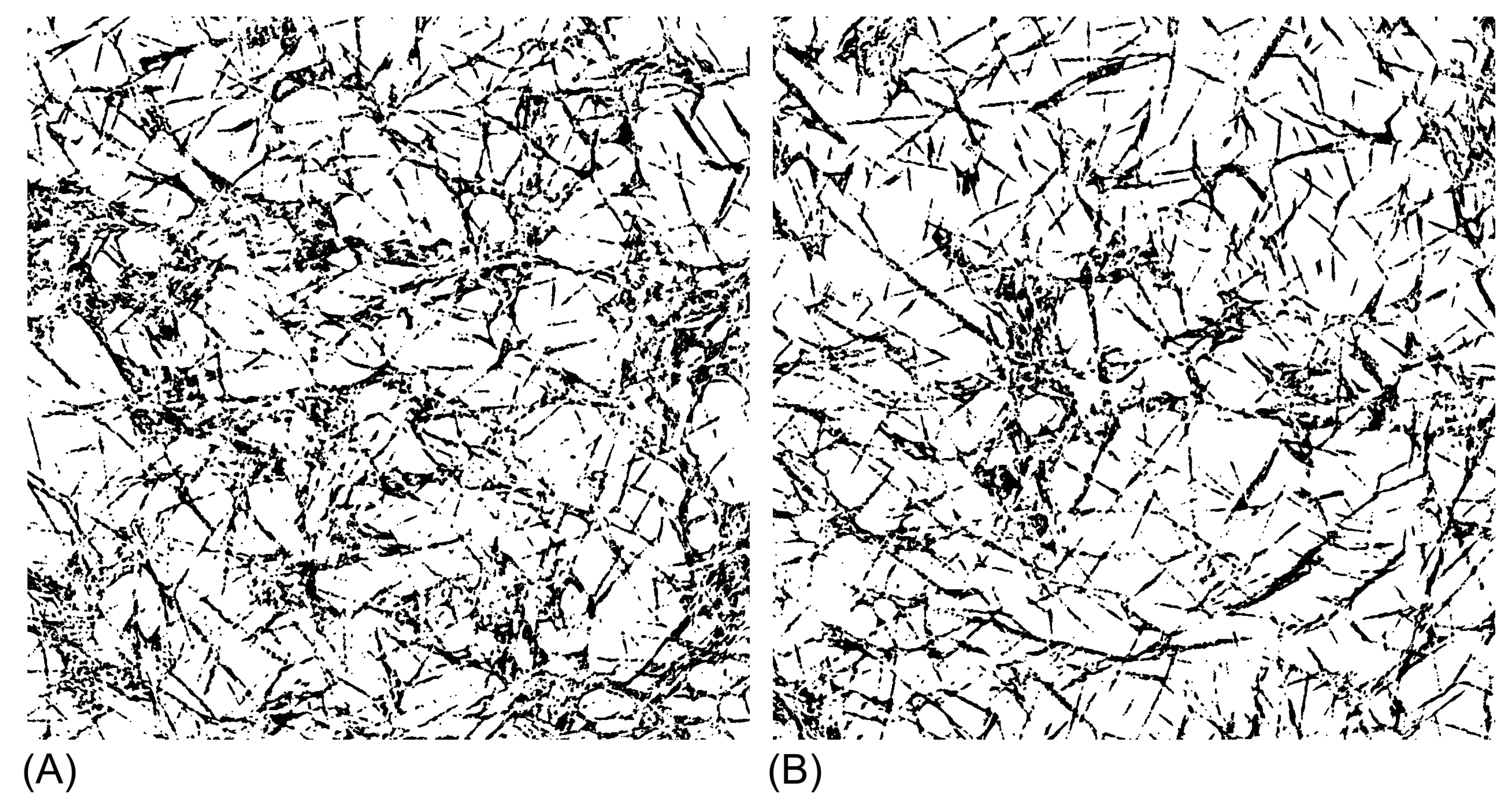
Figure 4.
Compressed images, taken from a Nano CT Zeiss Xradia Versa 420; A) Schematic arrangement in the compression device with GDLs on the channel (R2) and block sides (R3), with BW image samples (not in scale); B) sample image from a nano CT Zeiss Xradia Versa 420.
Figure 4.
Compressed images, taken from a Nano CT Zeiss Xradia Versa 420; A) Schematic arrangement in the compression device with GDLs on the channel (R2) and block sides (R3), with BW image samples (not in scale); B) sample image from a nano CT Zeiss Xradia Versa 420.
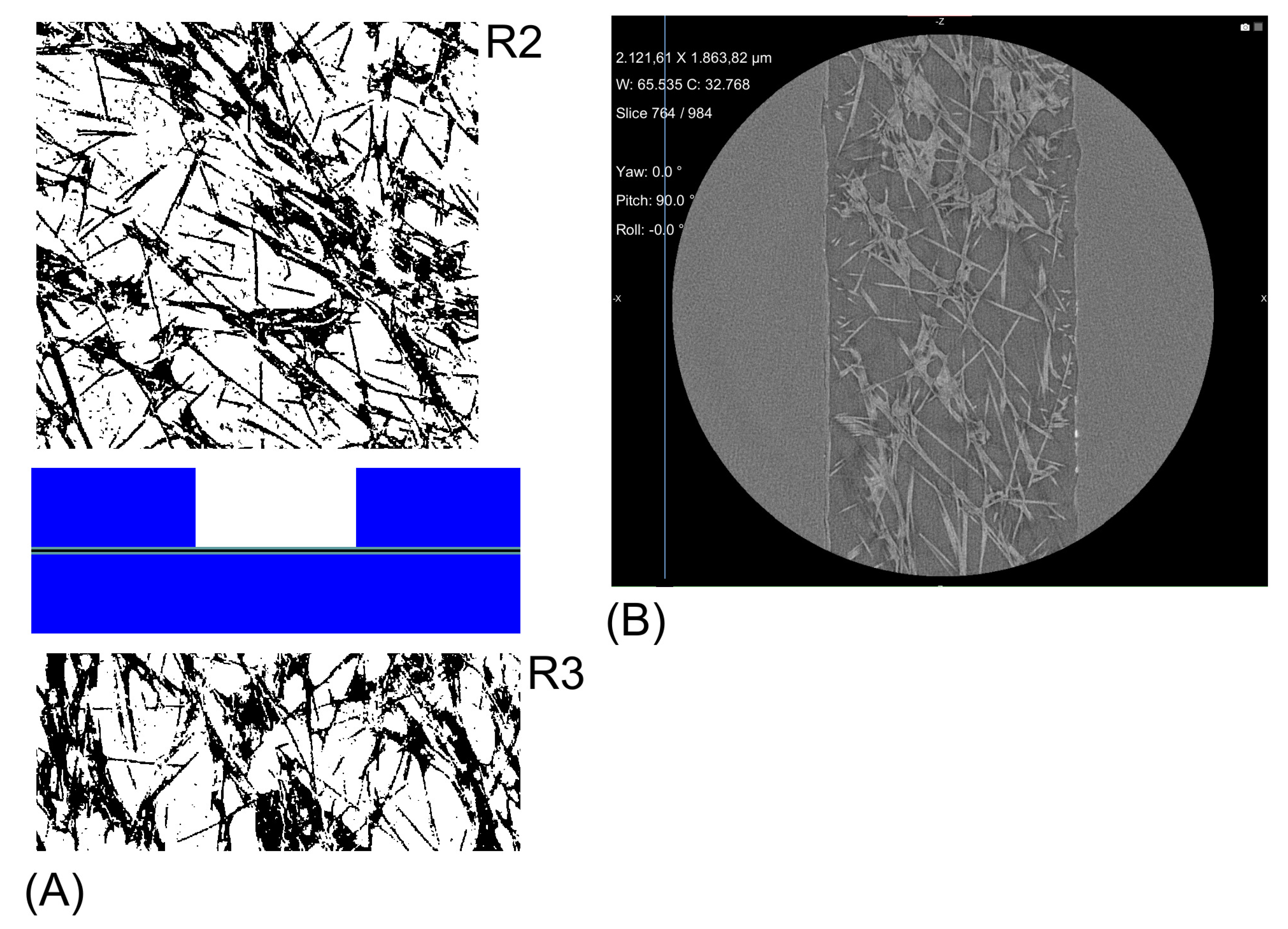
Figure 5.
Images from real Toray data under a flow field with 1.0 mm channel width, series R2: A) 6% compression, image No. 5 of 40; B) 6% compression, image No. 20 of 40; C) 6% compression, image No. 24 of 40; D) 6% compression, image No. 26 of 40.
Figure 5.
Images from real Toray data under a flow field with 1.0 mm channel width, series R2: A) 6% compression, image No. 5 of 40; B) 6% compression, image No. 20 of 40; C) 6% compression, image No. 24 of 40; D) 6% compression, image No. 26 of 40.
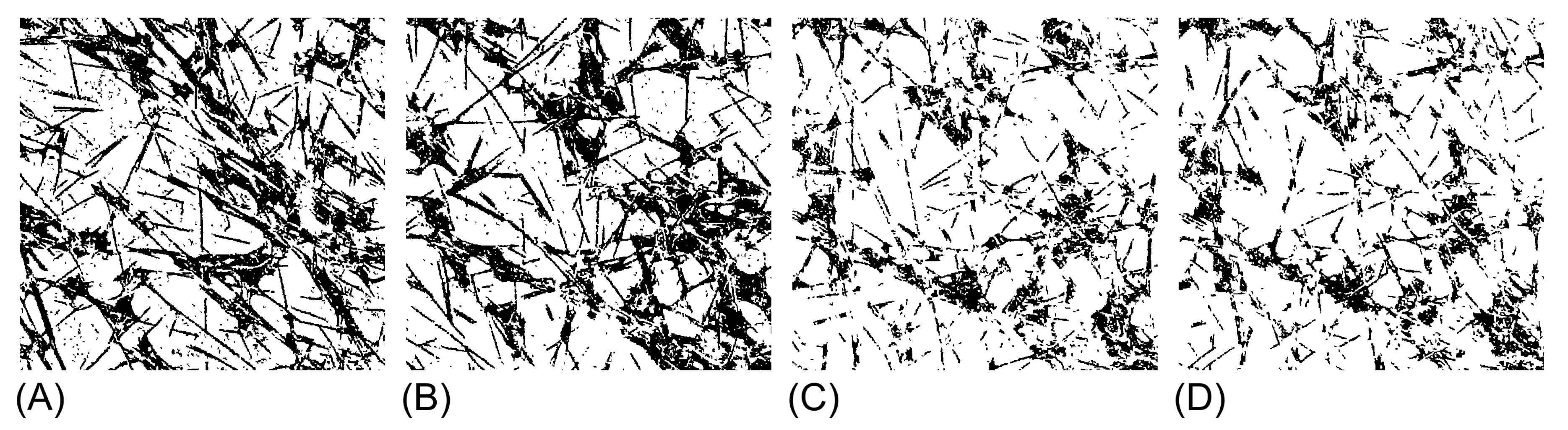
Figure 6.
Images from real Toray data under a flow field with 0.8 mm channel width, series R3: A) 7% compression, image No. 1 of 40; B) 7% compression, image No. 2 of 40; C) 7% compression, image No. 13 of 40; D) 7% compression, image No. 18 of 40.
Figure 6.
Images from real Toray data under a flow field with 0.8 mm channel width, series R3: A) 7% compression, image No. 1 of 40; B) 7% compression, image No. 2 of 40; C) 7% compression, image No. 13 of 40; D) 7% compression, image No. 18 of 40.
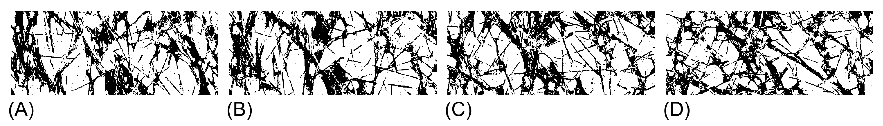
Figure 7.
Demonstration of image compression: 50% compression results in pairwise merging of two BW images to one gray level one. Three gray level images were merged from six BW images; B) images 23 to 28 of a stack with = ; D) images 23 to 28 of a stack with , annotation as in Figure 2.
Figure 7.
Demonstration of image compression: 50% compression results in pairwise merging of two BW images to one gray level one. Three gray level images were merged from six BW images; B) images 23 to 28 of a stack with = ; D) images 23 to 28 of a stack with , annotation as in Figure 2.
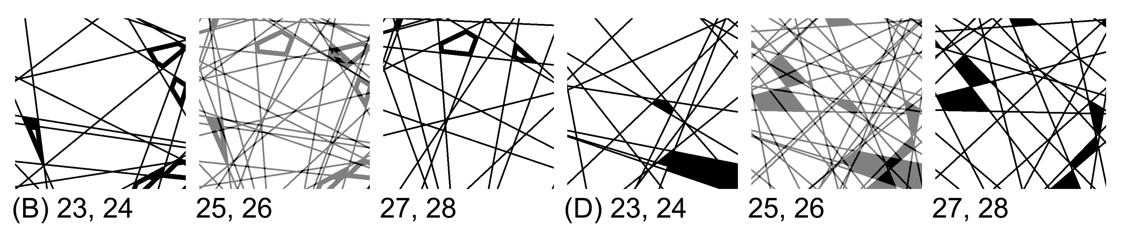
Figure 8.
Training history, fold 4.
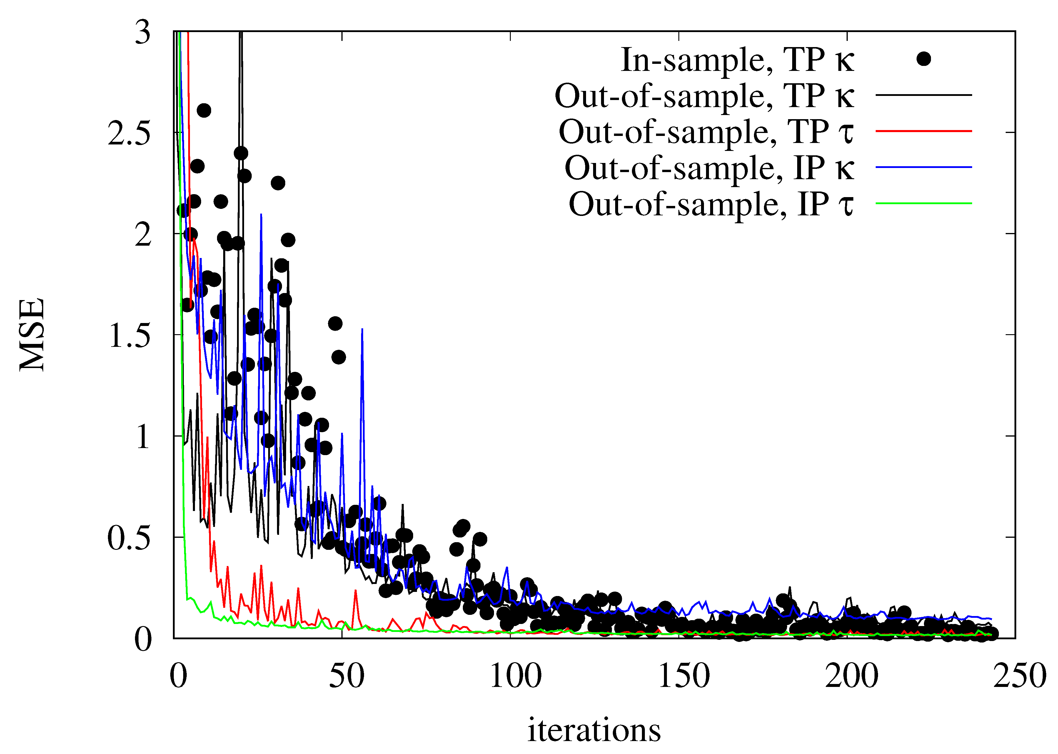
Figure 9.
Three layers of the CNN during the prediction of an image stack. The images are not to scale.
Figure 9.
Three layers of the CNN during the prediction of an image stack. The images are not to scale.
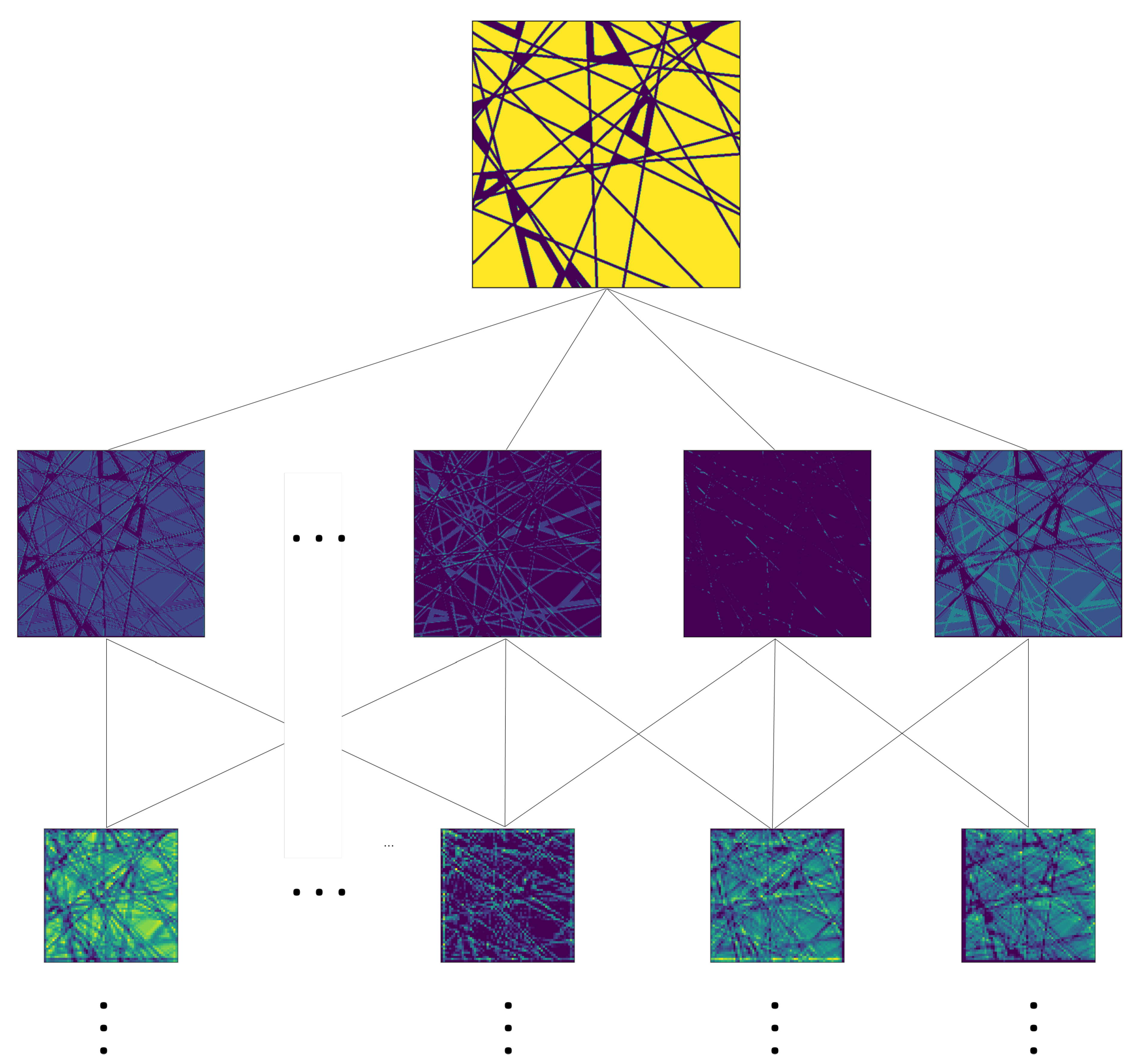
Figure 10.
Accuracy of the predicted permeability and tortuosity for different binder widths , uncompressed; a) TP ; b) IP ; c) TP ; and d) IP .
Figure 10.
Accuracy of the predicted permeability and tortuosity for different binder widths , uncompressed; a) TP ; b) IP ; c) TP ; and d) IP .
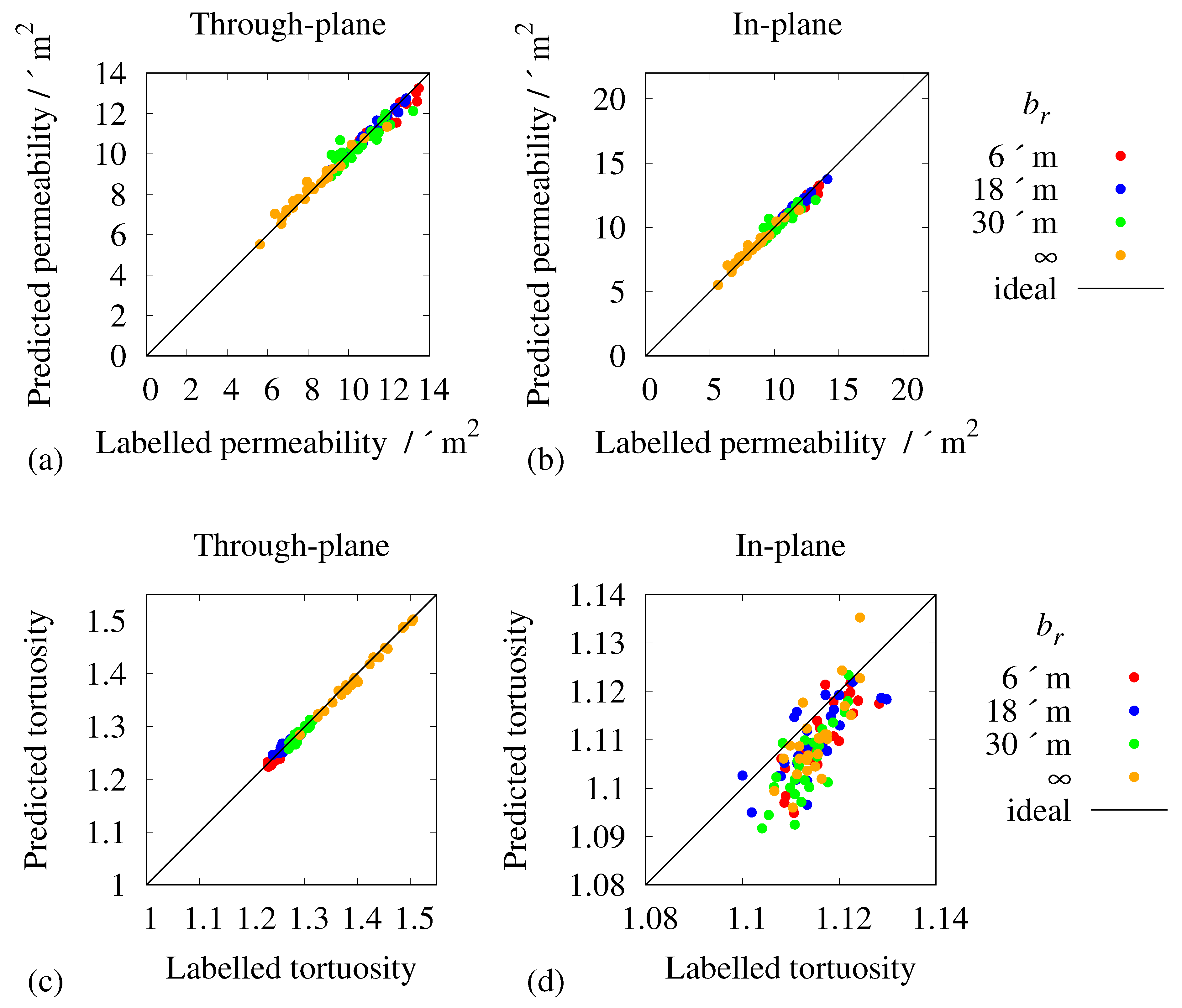
Figure 11.
Permeability of the compressed GDL, series R2, calculated with LB simulations and predicted by the CNN.
Figure 11.
Permeability of the compressed GDL, series R2, calculated with LB simulations and predicted by the CNN.
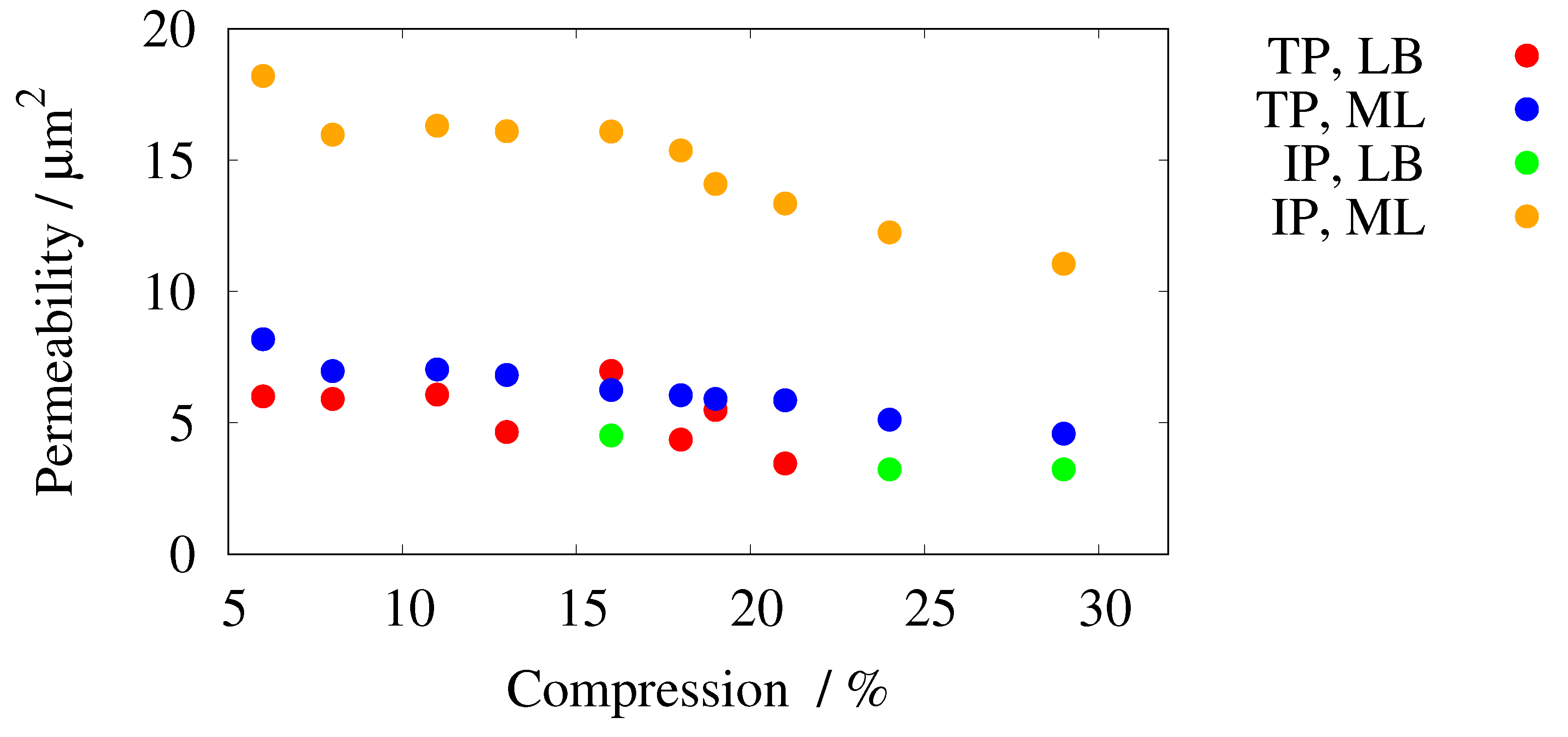
Figure 12.
Permeability of the compressed GDL, series R3, calculated with LB simulations and predicted by the CNN.
Figure 12.
Permeability of the compressed GDL, series R3, calculated with LB simulations and predicted by the CNN.
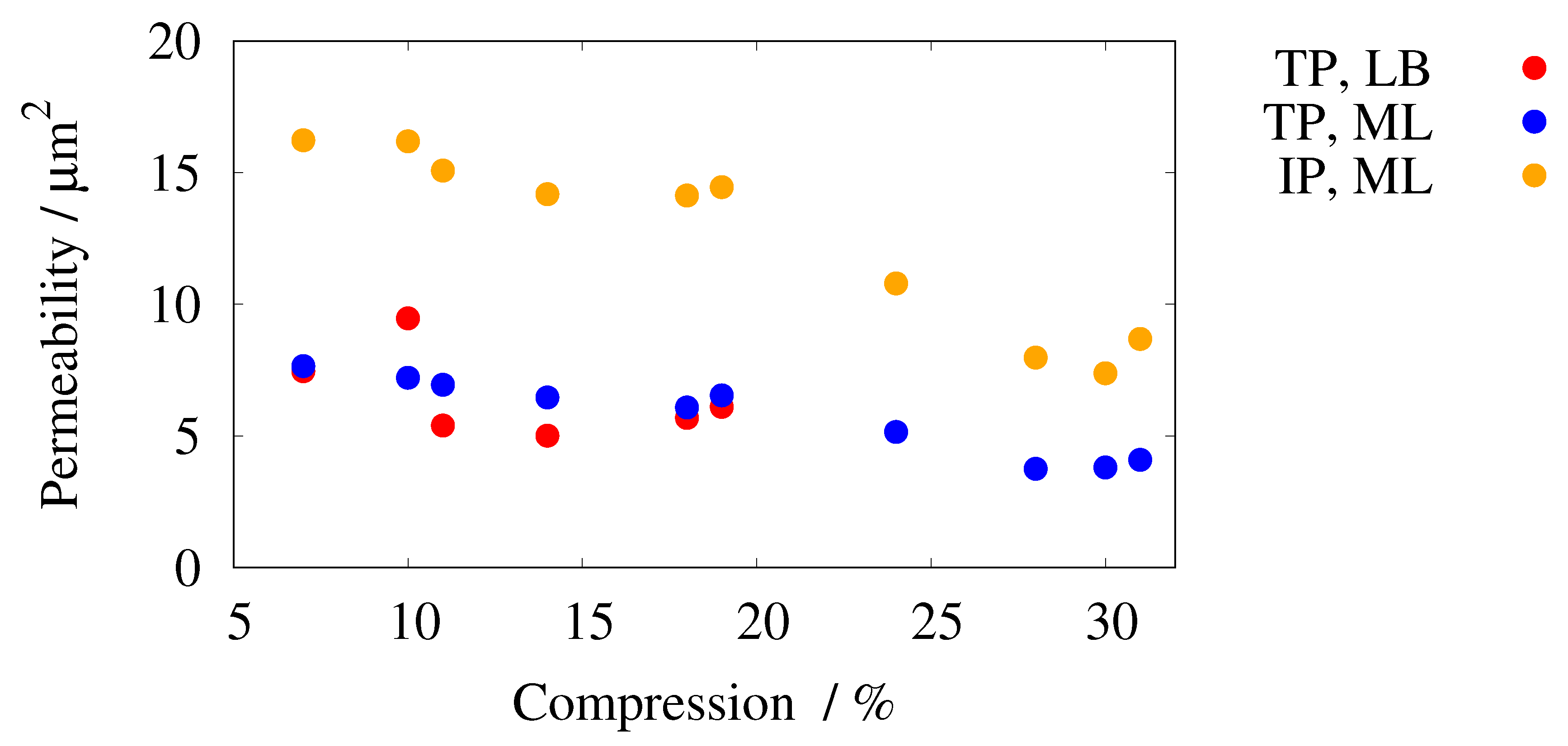
Figure 13.
Consistency of the predicted values of the R2 data with the Kozeny–Carman (KC) trend.
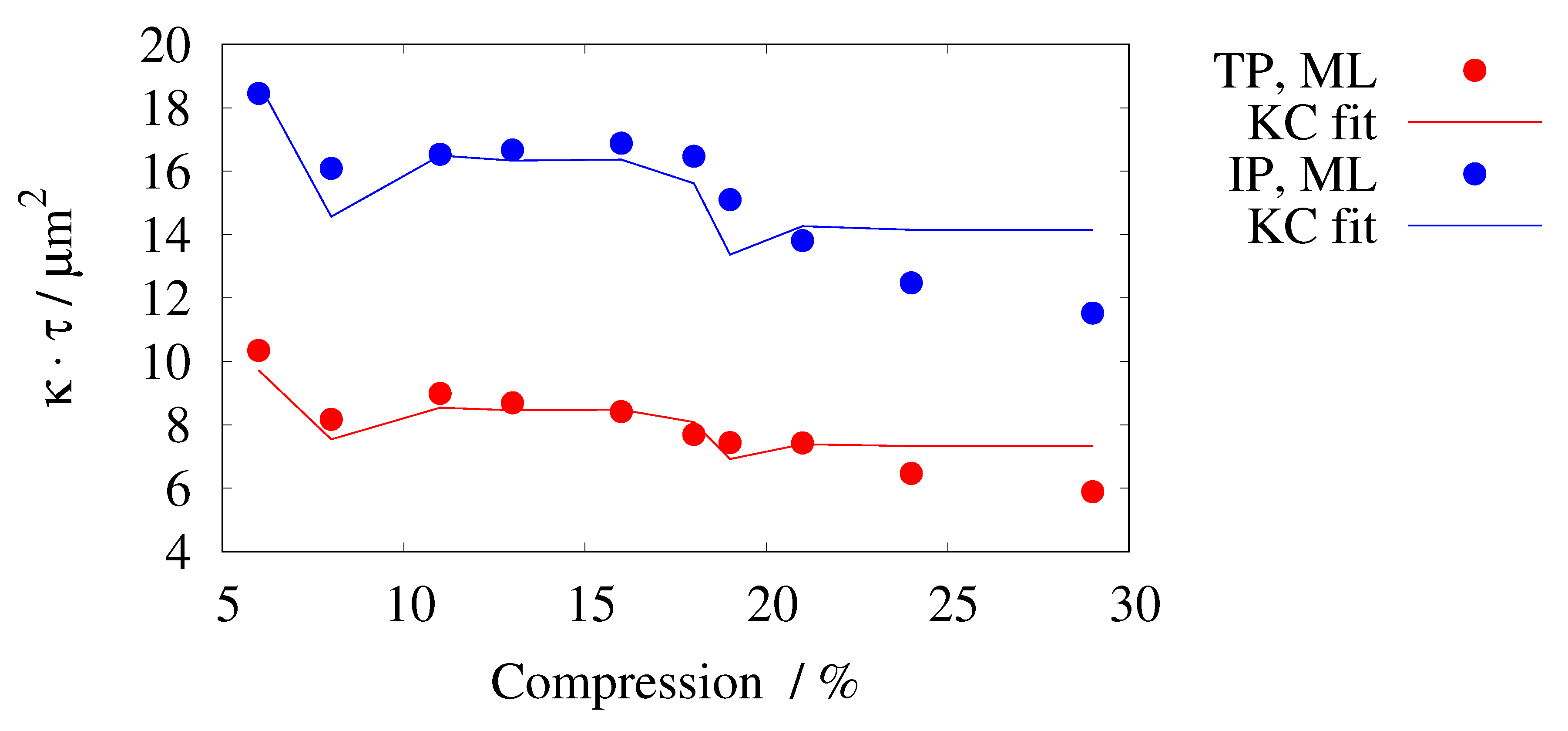
Figure 14.
Consistency of the predicted values of the R3 data with the Kozeny–Carman (KC) trend.
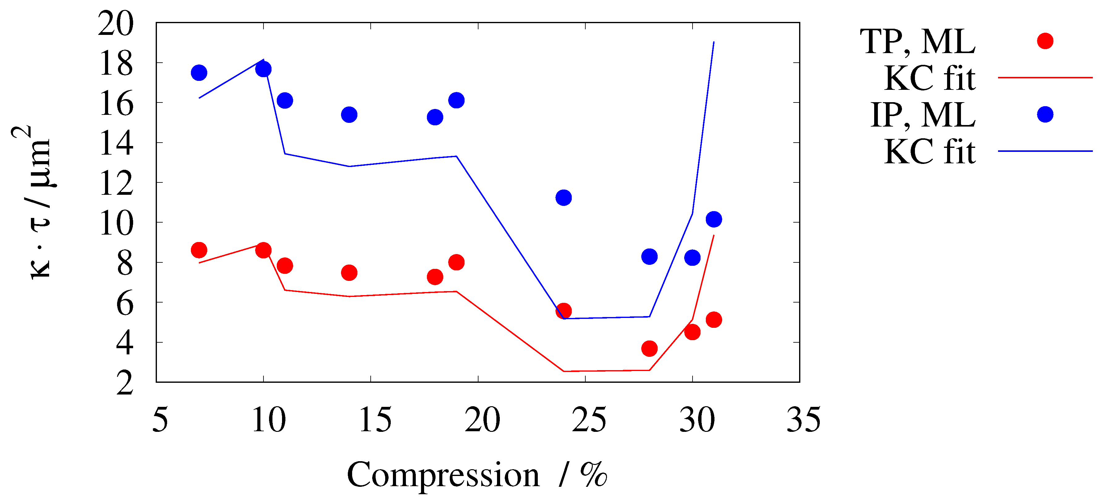

Table 1.
Dimensions of the images series R1, R2, and R3.
| Series | No. | Comp. | No. of | Dimensions |
| % | images | |||
| R1 | 1 | 0 | 200 | 1250x1250 |
| R2 | 1 | 6 | 40 | 694x670 |
| 2 | 8 | 22 | 671x688 | |
| 3 | 11 | 27 | 697x661 | |
| 4 | 13 | 40 | 684x673 | |
| 5 | 16 | 22 | 682x682 | |
| 6 | 18 | 40 | 673x687 | |
| 7 | 19 | 21 | 685x680 | |
| 8 | 21 | 40 | 688x677 | |
| 9 | 24 | 40 | 670x685 | |
| 10 | 29 | 40 | 670x685 | |
| R3 | 1 | 7 | 40 | 760x310 |
| 2 | 10 | 40 | 760x310 | |
| 3 | 11 | 40 | 760x310 | |
| 4 | 14 | 40 | 760x310 | |
| 5 | 18 | 40 | 760x310 | |
| 6 | 19 | 40 | 760x310 | |
| 7 | 24 | 40 | 760x310 | |
| 8 | 28 | 40 | 760x310 | |
| 9 | 30 | 40 | 760x310 | |
| 10 | 31 | 40 | 760x310 |
Table 2.
Tortuosity and permeability of 50 sub-sections of real data of series R1, predicted by the CNN, were trained with fold no. 4. The physical units of the variance are the square of the units in the column headers. The lower section shows the characteristics of the training data.
Table 2.
Tortuosity and permeability of 50 sub-sections of real data of series R1, predicted by the CNN, were trained with fold no. 4. The physical units of the variance are the square of the units in the column headers. The lower section shows the characteristics of the training data.
| TP | IP | |||||
| min | 8.89 | 1.17 | 11.73 | 17.44 | 1.07 | 19.23 |
| max | 11.94 | 1.36 | 15.18 | 19.82 | 1.14 | 22.02 |
| average | 10.54 | 1.27 | 13.43 | 18.83 | 1.10 | 20.80 |
| median | 10.54 | 1.28 | 18.85 | 1.10 | ||
| std. deviation | 0.62 | 0.038 | 0.75 | 0.56 | 0.014 | 0.69 |
| variance | 0.38 | 0.32 | ||||
| var. coeff. | ||||||
| average (B) in [24] | 11.18 | 1.27 | 17.98 | 1.11 | ||
| average (C) in [24] | 10.51 | 1.29 | 17.81 | 1.11 | ||
| favored: | C | B | B | B, C | ||
Table 3.
The tortuosity and permeability of real data, predicted by the CNN, trained with fold no. 4. The series are annotated according to Section 2.5.
Table 3.
The tortuosity and permeability of real data, predicted by the CNN, trained with fold no. 4. The series are annotated according to Section 2.5.
| Series | No. | Comp. | Porosity | TP | IP | |||||||
| % | ||||||||||||
| R2 | 1 | 6 | 0.688 | 7.12 | 1.22 | 1.26 | 6.01 | 8.18 | 1.01 | 18.20 | ||
| 2 | 8 | 0.666 | 6.38 | 1.13 | 1.17 | 5.91 | 6.97 | 1.01 | 15.97 | |||
| 3 | 11 | 0.678 | 6.72 | 1.15 | 1.28 | 6.07 | 7.03 | 1.01 | 16.31 | |||
| 4 | 13 | 0.669 | 6.74 | 1.23 | 1.27 | 4.65 | 6.82 | 1.04 | 16.10 | |||
| 5 | 16 | 0.669 | 6.74 | 1.11 | 1.35 | 6.98 | 6.25 | 1.05 | 16.09 | |||
| 6 | 18 | 0.669 | 6.59 | 1.25 | 1.27 | 4.36 | 6.05 | 1.07 | 15.37 | |||
| 7 | 19 | 0.680 | 6.05 | 1.12 | 1.26 | 5.49 | 5.91 | 1.07 | 14.09 | |||
| 8 | 21 | 0.644 | 6.42 | 1.26 | 1.27 | 3.46 | 5.86 | 1.03 | 13.35 | |||
| 9 | 24 | 0.640 | 6.41 | 1.27 | 1.27 | 3.23 | 5.12 | 1.02 | 12.25 | |||
| 10 | 29 | 0.640 | 6.41 | 1.27 | 1.28 | 3.23 | 4.59 | 1.04 | 11.05 | |||
| R3 | 1 | 7 | 0.685 | 7.61 | 1.18 | 1.13 | 7.46 | 7.65 | 1.08 | 16.23 | ||
| 2 | 10 | 0.709 | 7.91 | 1.15 | 1.19 | 9.46 | 7.21 | 1.09 | 16.19 | |||
| 3 | 11 | 0.669 | 7.02 | 1.20 | 1.13 | 5.39 | 6.94 | 1.07 | 15.08 | |||
| 4 | 14 | 0.666 | 6.86 | 1.20 | 1.16 | 5.01 | 6.46 | 1.09 | 14.18 | |||
| 5 | 18 | 0.678 | 6.91 | 1.18 | 1.20 | 5.68 | 6.08 | 1.08 | 14.13 | |||
| 6 | 19 | 0.685 | 6.89 | 1.18 | 1.22 | 6.54 | 1.11 | 14.45 | ||||
| 7 | 24 | 0.597 | 4.61 | 1.08 | 5.15 | 1.04 | 10.79 | |||||
| 8 | 28 | 0.555 | 4.84 | 0.98 | 3.75 | 1.04 | 7.97 | |||||
| 9 | 30 | 0.570 | 6.69 | 1.19 | 3.80 | 1.12 | 7.38 | |||||
| 10 | 31 | 0.592 | 8.87 | 1.25 | 4.09 | 1.17 | 8.68 | |||||
Disclaimer/Publisher’s Note: The statements, opinions and data contained in all publications are solely those of the individual author(s) and contributor(s) and not of MDPI and/or the editor(s). MDPI and/or the editor(s) disclaim responsibility for any injury to people or property resulting from any ideas, methods, instructions or products referred to in the content. |
© 2023 by the authors. Licensee MDPI, Basel, Switzerland. This article is an open access article distributed under the terms and conditions of the Creative Commons Attribution (CC BY) license (http://creativecommons.org/licenses/by/4.0/).
Copyright: This open access article is published under a Creative Commons CC BY 4.0 license, which permit the free download, distribution, and reuse, provided that the author and preprint are cited in any reuse.


