Submitted:
28 April 2023
Posted:
04 May 2023
Read the latest preprint version here
Abstract
High-precision ground point cloud data has a wide range of applications in various fields, and the separation of ground points from non-ground points is a crucial preprocessing step. Therefore, designing an efficient, accurate, and stable ground extraction algorithm is of great significance for improving the processing efficiency and analysis accuracy of point cloud data. The study area in this article was a Park in Guilin, Guangxi, China. The point cloud was obtained by utilizing the UAV platform. In order to improve the stability and accuracy of the Filter algorithm, this article proposed a triangular grid filter based on Slope Filter, found violation points by the spatial position relationship within each point in the triangulation network, improved KD-Tree-Based Euclidean Clustering, and applied it to the non-ground points extraction, this method has good accuracy, stability and achieves good results in separating ground points from non-ground points. At first, using Slope Filter to remove some non-ground points, to reduce the error of taking ground points as non-ground points; Secondly, established a triangular grid based on the triangular relationship between each point, the violation-triangle can determin through the grid, and then the corresponding violation points were found in the violation-triangle; Thirdly, according to the three-point collinear method to extract the regular points, used these points to extract the regular landmarks by KD-Tree-Based Euclidean Clustering and Convex Hull Algorithm; Finally, removed disperse points and irregular landmarks by Clustering Algorithm. In order to confirm the superiority of this algorithm, this article compared the filter effects of various algorithms on the study area and filtered the 15 sample data provided by ISPRS, and obtained an average error of 3. 46%. The results showed that the algorithm in this article have a high processing efficiency and accuracy, which can greatly improve the processing efficiency of point cloud data in practical applications.
Keywords:
Slope Filter
; point cloud
; triangular grid
; KD-Tree-Based Euclidean Clustering
1. Introduction
Airborne Lidar technology combines global positioning system, laser scanner and inertial navigation system, which can obtain high-precision ground point cloud data quickly and efficiently[1]. Airborne Lidar point cloud data is an important data source for obtaining spatial three-dimensional information. Because of its ability to accurately express the location of ground objects, it is widely used in many fields such as constructing digital elevation model (DEM), contour production, and three-dimensional model generation. However, due to the massive and disordered characteristics of point cloud data, the classification and feature extraction of point cloud data is particularly important, point cloud filter is undoubtedly an important step in it.
There are many scholars have compared the current mainstream filter algorithms. Sithole used 8 Filter algorithms to filter different point cloud data and compared their errors, they concluded that the adaptive irregular triangulation filter method has the best filter effect [2]. Zou compared and analyzed three commonly used filter methods from both qualitative and quantitative aspects, and obtained the most suitable point cloud filter algorithm for different terrain data [3]. From the above, it can be seen that the point cloud Filter algorithm has received extensive attention from scholars.
At present, the commonly used point cloud filter algorithms mainly include Segmentation-Based Filtering, Cloth Simulation Filter, and Slope Filter algorithm[4]. The progressive triangulation filter algorithm is proposed by Lin, the principle is to select the lowest point in the local area as the seed point of TIN, and then used the remaining points to iteratively encrypt the triangular mesh[5]. However, this method usually cannot preserve the points on the scarp when meeting steep slopes, it will misjudge the non-ground points close to the ground as ground points. The Cloth Simulation Filter is proposed by Zhang, the principle is to flip the original point cloud data up and down, and then projected the flipped point cloud data and cloth node simulated to the same horizontal plane, found the point corresponding to each node in the cloth and recorded the height of the corresponding point before projection, finally, compared the distance between the laser point cloud and the cloth node in the same horizontal coordinate, if the distance exceeds the set threshold, marked it as a non-ground point, otherwise it is marked as a ground point[6]. The Cloth Simulation Filter has five adjustable parameters to complete the point cloud filter work. In the actual filter process, the filter effect is mainly improved by modifying the two parameters of grid resolution and cloth hardness, but the Cloth Simulation Filter has poor filter effect in the face of multi-storey buildings. The Slope Filter is proposed by Vosselman, the principle is to distinguish ground points and non-ground points according to the difference of slope [7], however, the method of fixed slope is not reasonable enough to be applied to the whole situation. On the basis of three commonly used Filter methods, many scholars have also proposed improvement methods. Sithole improves the Slope Filter, the slope threshold can change with the terrain, which enhances the applicability of the algorithm[2], this method requires multiple parameters to be set manually , in order to improve the accuracy, efficiency and adaptability of the point cloud filter, Zhu also proposed an adaptive threshold point cloud filter method based on multi-level moving surface fitting [8], this algorithm can obtain good filter effect in complex and continuous terrain areas, but the filter effect in discontinuous terrain areas needs to be improved. Wang also proposed a Multi-scale Adaptive Point Cloud Slope Filter method based on Slope Filter. This method referenced on the idea of multi-scale virtual network and used distance weighting to realize multi-scale adaptive point cloud slope Filter[9], however, this method is less stable than triangulation filter in urban scene areas.
This article got the non-ground points by finding the violation points and using these points for KD-Tree-Based Euclidean Clustering, the non-ground features are expressed in the form of cluster points. There are many scholars have studied the extraction of objects by clustering methods, Region growing[10] and K-means algorithms[11] have been employed for direct clustering in the 3-D model[12].Rodriguez and Laio proposed a clustering by fast search and find of density peaks[13], Chen applied the exponential function density clustering method to indoor objects extraction and achieved good results[14]. These researches showed that it is feasible to use clustering algorithm for objects extraction. Sun used the hierarchical Euclidean Clustering to extract the building rooftop patches[Error! Reference source not found.], Guo used KD-Tree-Based Euclidean Clustering for point cloud extraction and segmentation[12], Gamal used DGCNN and Euclidean Clustering to finish the segmentation of Lidar buildings[16], these researches are proved that the Euclidean Clustering method is feasible for the extraction of regular buildings, and KD-Tree-Based Euclidean Clustering can increase the clustering operation speed, this method can be applied to the segmentation of large scene point clouds, so this article proposed an extraction method for regular landmarks by using KD-Tree-Based Euclidean Clustering, by calculating the violation point and collinear judgment to reduce the number of seeds that need index, and the calculation amount is reduced.
Therefore, this article proposed a triangular mesh filter method based on Slope Filter(Figure 1). At first, using Slope Filter to remove some non-ground points to reduce the error of taking ground points as non-ground points; Secondly, established a triangular grid based on the triangular relationship between each point, the violation-triangular can determin through the grid, and then the corresponding violation points were found in the violation triangle; Thirdly, according to the three-point collinear method to extract the regular points, used these points to extract the regular landmarks by KD-Tree-Based Euclidean Clustering and Convex Hull Algorithm; Finally, removed disperse points and irregular landmarks by Clustering Algorithm.
2. Algorithm Principle
2.1. Data Preprocessing
Due to factors such as the number of echoes set and occlusion during point cloud acquisition, the point cloud density may be too high or too low. Therefore, before processing point cloud data, resampling is required. Resampling can be divided into up-sampling and down-sampling, down-sampling involves extracting signals, while up-sampling involves interpolating signals. This experiment mainly explores point cloud Filter, so the research data only needed to be down-sampled, in this article, we used setting distance to down-sample point cloud data. Specifically, we divide the point cloud data into a three-dimensional grid, and keep everyone point in each grid, through down-sampling, point cloud density can be reduced, the calculation during subsequent filter processes can be reduced, and improved the calculation speed. During the working process of Lidar, abnormal noise points may be generated due to various factors such as wind, water vapor, and illumination. This article used Statistical Filter method to remove the noise points, the principle is to calculate the average distance from each point to its neighboring points, and determined the distance threshold based on the normal distribution. If is less than , the point was considered an interior point and kept. If is more than , the point was considered a noise point and removed.
2.1. Slope Filter
Slope is a variable representing the degree of surface undulation, the meaning of Slope Filter is to judge whether the grid slope value in the set grid is within the set range, and on this basis to determine whether the grid is a ground point. This method was first proposed by Vosselman and then improved by Sithole to make the method suitable for steep terrain, the principle of slope Filter method is to establish a two-dimensional grid for the whole test area, each grid records the lowest point elevation of the internal storage point cloud to obtain the elevation grid(Figure 2), obtain elevation values within a two-dimensional horizontal grid in sequence(Figure 3), and then calculate the slope value within the grid(, Equation(1)), judging the attributes of the grid sequentially(Figure 4)and extracting the point cloud with the ground attribute. If the height difference between the point cloud and lowest point in the grid is within the threshold, the point cloud can be considered the ground points.
are the grid positions with lower elevation and their corresponding elevation values in the elevation grid; are the grid positions with higher elevation and their corresponding elevation values in the elevation grid.
2.1. Constructing a triangular grid and identifying violation points.
The Delaunay triangulation method is used to construct a triangular mesh for point clouds in this article, it has the properties of empty circumcircles and maximum minimum angles[17], in other words, the circumcircle of either triangle is empty for two adjacent triangles, it means don’t have any points contained. In this way can avoid the generation of elongated triangles, and this method is widely used in 3D modeling, low poly modeling, facial construction fields [18], the triangular grid is constructed by this method in this article(Figure 5). It is found that there is no elongated triangle in the internal triangular grid except for the narrow triangle generated by cutting the point cloud area at the boundary, after generating the triangular grid, it is necessary to judge the positional relationship between the triangles in the grid, acquiring each triangle attribute in turn, and if there is a common edge between two triangles, it can be considered that the two triangles are adjacent, for triangles on the boundary, if the number of adjacent triangles is less than 3, the triangle is considered a boundary triangle, in order to reduce the computational workload in the iterative process, skip judgment violation point. then calculate the angle between the adjacent triangles in sequence. The process is as follows:
- (1)
- Calculating the normal vector of adjacent triangles in sequence by the calibration number of triangles(, Equation(2)), then substitute coordinates into (2) to get surface normal vector(, Equation(3)).
- (2)
- According to the angle between two planes is equal to the angle between normal vectors of two planes to obtain the angle between two triangles(, Equation(4)).
- (3)
- Judging the angle and longest side length of each triangle with threshold, if them are more than the threshold range, the selection of threshold angle and side length of 70°and 4 m can realize the extraction of most scene violation points, mark these triangles as violation triangles, if not, continue until judge all triangles.
- (4)
- Extracting the maximum value of each violation triangles as violation points.
2.4. Collinear judgment
The collinearity detection algorithm mainly relies on the slope between two points to make the determination[19], this method is applied to the contour extraction of buildings[20,21], the algorithm follows these steps: First, a point randomly selected from violation points as the center of the circle, and then find two other points that are closest to this point, next, calculate the slopes of two lines that connect two points to the center point, and compare them to the slope between the two outliers(m, Equation(5)). If the absolute difference between these two slopes is less than threshold, it is considered that these three points are collinear.
is angle difference between two of the three points, are the abscissa of three points,are the ordinate of three points .
2.5. Cluster Point Classification
This article used KD-Tree-Based Euclidean Clustering to distinguish violation points, the principle is that if the distance between points is less than the threshold, it means that the two points are locally connected to the same point set. If the distance between points is more than the distance, it means that the two points are locally connected and do not belong to the same point set(Figure 6). In this article,the detail process is as follows(Figure 7):
- (1)
- Select a point from the regular violation point set T which judged by the collinear judgment as the cluster center point.
- (2)
- Do a neighbor point index based on KD-Tree for the original point cloud data.
- (3)
- Find the points within the distance threshold and add these points to the undetermined set P.
- (4)
- Check whether the number of points in p increases or height difference overrun,if is,repeated steps 2-3 until the number of points in P does not increase.
- (5)
- Output P set and removed P from Q.
- (6)
- Remove the points that are repeated with P from T to avoid repeated operations to increase the amount of calculation.
- (7)
- Check whether all the points in T had calculated and repeat steps 2-6 until there are unoperated points.
3. The Procedure of Experiment
3.1. Experimental Data and Evaluation Criteria
The study area in this article is a Park in Guilin, Guangxi, China(Figure 8). the point cloud was obtained by utilizing the UAV platform. This article adopted the filter error evaluation criteria proposed by ISPRS in 2003, which includes Type I error, Type II error, and total error. Type I error is the error of misclassifying ground points as non-ground points, while Type II error is the error of misclassifying non-ground points as ground points, the total error is the ratio of the two types of errors to the total number of points in the point cloud(Table 1).
3.2. The Process of Triangulation Method Filter
Selecting a representative and diverse area to verify the algorithm of this article(Figure 9)The study area contains various types of scene elements, such as dense forests, buildings and steep slopes. The terrain in this area is uneven and the buildings are multistory and irregular, it means that a more stringent test for point cloud filter algorithms. At first, constructing a triangular grid for the study area(Figure 5), then, determining the adjacent relationships between triangles in the gird and get the angles of each adjacent triangles by the cross product of vectors, comparing the angles of each adjacent triangles and threshold, if the angle exceed the threshold range, mark two triangles about this angle as violation triangles, on this basis, get the longest edge expect the common edges of violation triangles, if the longest edge exceed threshold, marking the highest point of the triangle which have the longest edge as regular violation points(Figure 10), based on the image of violation points, it can be seen that the Triangulation Grid Algorithm can roughly extract the outline of the buildings based on the distance and angle, then, using the three-point collinearity method to determine whether the regular violation points are collinear, if they are collinear, marking these point until traverse all regular violation points. In this image(Figure 11), it can be seen that the outer contour of the building, however there are still some forest points mixed in what are judged as regular violation points, these points will be removed in the subsequent clustering step. Then using these regular violation points as centers, clustering the original point cloud by the distance of each points, this article used different colors to represent the point groups after Euclidean Clustering(Figure 12). In detail, at first, selecting a point from the regular violation points, take this point as clustering center and take the clustering threshold to find the cluster group of this point, of course, it is necessary to set an elevation threshold,the elevation threshold of 3 m can achieve most scenes, in order to prevent the ground points within the threshold range added to the clustering group as non-ground points, after completing the clustering grouping of this point, removing the regular violation points which in the group to avoid repeated operations, then, repeat above process until all regular points have obtained their group. Finally, traversing the number of points in each groups, retaining the group which the number of points exceed the set value, the steep point may be used as the violation point when extracting, because the steep point is connected to the ground,the number of points after clustering is the largest, by limiting the number of points after clustering, the steep points are avoided as non-ground points, then removing the group if the number of points is less than the set value, The reasons for this situation are:
- (1)
- There are several separate points in the same area, and the distance between them also within the distance threshold, this situation needs to remove, because it will be easy to remove the ground points between these separate points.
- (2)
- The points in the group may be due to the collinear situation of some forest points, because the forest is roughly uneven, and this is a reason why set an elevation value, these group may be composed of forest points that are misjudged as regular violation points and forest points close to them.
It is necessary to establish the outer contour of the ground objects in the first non-ground points extraction process. The process is to use the outer contour to warp the non-ground objects, in this process, some non-ground points that are not identified by the clustering method are also wrapped into the non-ground point clusters,such as the points inside the house, based on this method,the calculation amount of the second non-ground points filter is also reduced. Using the Convex Hull Algorithm to find the boundry of these clustering groups(Figure 13), then, finding the points located in the boundry from the original point and removing them, these removed points are non-ground points.
After removing some non-ground points, generate a new three-dimensional grid and repeat the previous process again to get violation points(Figure 14). However, unlike the previous process, it is necessary to reduce the screening conditions for the second screening violation points, and removed the screening condition of distance, because the screening condition of distance will take the non-ground points adjacent close to the ground as the ground points, not only that, reducing the threshold of the clustering distance in the point cloud clustering process, because the second round of screening is mainly aimed at scattered and irregular points, so use lower clustering distance is more appropriate. After completing the above process, the purpose of separating ground points from non-ground points is achieved, the blue points in the image are the original points of the study area, the red points are the points after Triangular Grid Filter. It can be seen that most of the non-ground points are separated from the original points, however, the clustering algorithm has limitations, it may misclassify some ground points which located in clusters of non-ground points as non-ground points, like the area marked(Figure 15), to address this issue , this article used Slope Filter before Triangular Grid Filter to extract ground points. Slope Filter classified low points with a slope attribute of ground as ground points and selected points located at height from the classified ground points as non-ground points. Slope Filter has limitations and can not adjust its slope threshold adaptively based on the terrain conditions, but it can complement triangular grid filter in this article to improve the filter efficiency and accuracy. This article used Slope Filter with high threshold to extract the ground points embedded in non-ground points(Figure 16), then using triangular grid filter to complete the separation of ground points and non-ground points(Figure 17). The blue points are the original points, the red points are the points after filter. It can be seen that the method combining two methods significantly improves the accuracy of ground points filter, the filter effect of the marked area has also been significantly improved, based on it, this article compared other popular filter algorithms with this article method(Figure 18-23). In these images, the study area after EMD Filter, most non-ground points were removed, but there are still three group non-ground points neglected(Figure 18). The study area after SMRF Filter, most non-ground points were removed, with the process of filter, some ground points also removed like the blue marked area, and there are some points in three red marked area were neglected(Figure 19); The study area after Segmentation-Based Filtering, most non-ground points were removed expect some non-ground points close ground, but there are still some non-ground points were neglected like the points in the red area(Figure 20). The study area after Slope Filter, there are many ground points were removed in the blue marked area, and many non-ground points were neglected in the red marked area, we can see that the traditional Slope Filter has been unable to apply to most scenes, especially in the presence of composite buildings(Figure 21). The study area after Cloth Simulation Filter, most non-ground points were removed, but there are still some non-ground points were left and with the process of Filter, many ground points located on slope scarp were removed(Figure 22). The study area after combining Slope Filter and Triangular Grid Filter, almost non-ground points were removed, especially the points of buildings, with the help of Slope Filter, some ground points in the forest were retained like the red marked area(Figure 23). From these images, The triangular grid filter method based on Slope Filter has the best effect.
3.3. Data Comparison
To verify the filter performance in this scene, this article compared the errors of the study area according to the ISPRS standards. From this table(Table 2), it can be seen that the method in this article achieved better results with other methods. This is because the building in the study area has complex multi-layered structures and most Filter algorithms are based on grid filter, when facing the non-ground points on multi-layered buildings, the points on the lower layers may be misclassified as ground points to lead the first type of error become large. As for Cloth Simulation Filter, the effect is affected by the cloth hardness, this method is easy to misclassify nearby buildings ground points as non-ground points. when only using the Triangular Grid Filter, in dense forest areas this method may remove ground points inside the convex hull boundary as non-ground points, leading to a large type I error, Slope Filter sets a threshold to filter out high-slope areas in dense forest areas, reducing type I error, therefore, the combination of Slope Filter and triangular mesh algorithm can achieve good filter results in this study area.
In order to verify the Filter effect of the algorithm in other scenarios, this article used the point cloud which standard dataset publicly released by ISPRS as the accuracy comparison dataset(Figure 24-38), in these figures, (a) is the filtered result figure, (b) is the detail method figure. In (a) ,the white points are the filtered result, the blue points are the ground points marked by the original point cloud,the red points are the non-ground points marked by the original point cloud. In (b), the white points are the ground points after filtered, the red points are type II error points,the blue points are type I error points. This article calculated type I error, type II error, and total error in each sample(Table 3), and comparing the total error with other methods(Table 4). In Sample 1-1, almost non-ground points were removed and most ground points were retained, expect some ground points closed to buildings after filter in this article, because these buildings on hillside are close to the ground points(Figure 24). In sample 1-2, almost non-ground points were removed and most ground points were retained, because some ground points are close to building points or vegetation points, these ground points were removed, the distance threshold was too large(Figure 25)In Sample 2-1, some ground points are removed, because there are some non-ground points are close to ground points of scene boundary, and the distance threshold was too large(Figure 26). In sample 2-2, there are some ground points were removed because these points are located on the slope, these points have too large inclination angle or at the boundary of the scene(Figure 27). In Sample 2-3, the points of bridge and buildings were removed, but there are some ground points were removed because these points are located on the slope, and these points closed to non-ground points(Figure 28). In Sample2-4, almost points of buildings and vegetation were removed, but there are some ground points were removed, because these points are close to non-ground points(Figure 29). In Sample 3-1, almost non-ground points were removed, but there are some ground points in buildings were removed, because these points are close to non-ground points that belonged to low buildings(Figure 30). In Sample 4-1, almost buildings are removed, but there are some ground points are removed, because these points are at the boundary of the scene and there is discontinuous terrain in the middle(Figure 31). In Sample 4-2, almost non-ground points were removed, but there are some ground points were removed because these points on the slope and closed to non-ground points(Figure 32). In Sample 5-1, almost non-ground points were removed, but there are some ground points were removed because these points are close to non-ground points, and the distance threshold is too large(Figure 33). In Sample 5-2, almost non-ground points were removed, but some ground points on the ridge were removed, because the angle between the points of the ridge is large and closed to the non-ground points(Figure 34). In Sample 5-3, almost non-ground points were removed, but the ground points on the slope were removed, because the angle between the points on the discontinuous slope is too large(Figure 35)In Sample5-4, almost non-ground points were removed, there are some ground points closed to non-ground points were removed, because the distance threshold is too large(Figure 36). In Sample 6-1, most non-ground points are removed, but there are some non-ground points were retained, because these non-ground points are close to a lot ground points, if remove these non-ground points will reduce filter efficiency and accuracy(Figure 37). In Sample 7-1, almost non-ground points were removed, but there are some ground points on the slope were removed, because the angle between the points on the slope is too large, these points were misjudged as non-ground point(Figure 38). By observing the filtered samples,the poor filter effect in each sample is found and marked, by amplifying the detail, it can be found that most of the poor filter is due to the misclassification of ground points as non-ground points. Above all, these samples showed that the method proposed by this article can complete the point cloud filter of most scenes, but some ground points will be misjudged as non-ground points, because the distance and angle thresholds cannot be adaptively changed. This is also the improvement direction of our follow-up plan.
With the compared of different methods, The type I, type II error and total error of the method proposed by this article are much smaller than other commonly filter methods in the study area , and the Filter effect is the best(Table 2). In 15 samples, the method proposed by this article can remove most of the non-ground points, but it will inevitably remove some ground points in the filter process, resulting in a large type I error. In addition,we found that the average of type II error is higher than type I error(Table 3), the main reason is that in the filtering process, there are several samples with a small mount of non-ground points, therefore, even if there are fewer non-ground points that are not identified in the filter process, it will lead to a large type II error, however, from the overall situation comparison, it can still found that type I error in most samples is greater than type II error. Comparing with the Filter methods proposed by other scholars, our method outperforms other methods in most scenarios expect, in addition to some scenarios, the average error is smaller than other methods, is 3. 68%(Table 4). In order to more intuitively see the error between different methods,we made the error comparison diagram of each samples(Figure 39),the result showed that the error in these samples is better than other methods except in the four samples,there are large number of near-ground points in these samples, it is easy to cause higher type I error, because the clustering threshold cannot be adaptively changed. Further analysis of the results, it is found that our method has a good effect in urban samples, compared with other methods, the total error is the smallest in urban samples expect sample 2-4, as for rural samples, our method is not the smallest in three samples, but the filter effect is not bad, so it can be seen that this method has a certain effect on the extraction of large scene buildings, and the extraction effect of scattered points and small objects is also good, from the range of curve changes in each scene,we can see that compared with other methods, the error amplitude of this method fluctuates little, the filter effect of each sample is relatively stable, and the error is controlled within 10%, it showed that this method has strong adaptability and can play a good filter effect for point cloud data in multiple scenes.
In order to more intuitively observe whether the ground point cloud after filter can be applied to practice, this article selected a sample from the urban and rural samples as the verification, and used the original data(Figure 40(a),41(a)), the ground data in the original data(Figure 40(b),41(b)), the filter data(Figure 40(c),41(c)) to make the surface reconstruction model.The result showed that the model generated by the filter points removed almost non-ground objects, and retained the geomorphological features on this basis, the generated terrain model is almost the same as the model composed of ground points, the results confirmed that the filter method in this article has certain utility, and can meet the requirements of point cloud filter.
4. Discussion
As an effective tool of point cloud filter, Slope Filter has been widely used in the classification of ground points and non-ground points, dividing the study are into grids is the first key step in this method. the ground grids and non-ground grids are distinguished by these grids, then, calculating the slope separately to get the lower points as the ground points. This article proposed a Filter method based on Slope Filter, obtaining the adjacent state between each points,get the information of distances and angles of each point, then calculate the violation points. The principle is that there must be a certain violation area between the non-ground area and the ground area, simply speaking, there will be an unnatural angle and distance area, unlike the ground slope will rise slowly at a certain natural angle, therefore, this article establishes a triangular grid to obtain the violation area, selecting two adjacent triangles in the gird, if the angle of these’ planes is too large, and the length of any edge in the two planes exceeds threshold, it can be determined that the triangle with the longest edge is the unnatural area, and then find the violation point from this triangle.
The large area usually uses airborne radar to obtain point cloud data, the characteristics of this method are that the horizontal of the points presents a certain distance distribution, it can be thought that if there is no contact with other objects in scanning, the points of same object often appear as a cluster point, based on this idea, this article adds KD-Tree-Based clustering algorithm to classify the objects in the scene,this method can express the distance relationship of each point,and is applied to the extraction of building point cloud, however, there are still some problems in point cloud filter, for point cloud with near-ground scattered point such as forest, it is easy to eliminate the ground points near the scattered points as non-ground points by using a large clustering threshold. So, this article proposed to use large threshold to extract higher non-ground points, most of these non-ground points are buildings. This article used a three-point collinear because these points are distributed regularly. after clustering and eliminating these regular violation points, using the lower threshold to eliminate scatter points. In the process of airborne radar scanning, it is inevitable to scan the building facade, because of this reason, this article added a height threshold to avoid the mutual conduction between the points in the clustering process and the ground points being eliminated.
Compared with using the grid, triangular grid can more accurately express the relationship between each point, it can filter non-ground points when facing multiple buildings with different heights, and determine whether the points are the ground points in the face of discontinuous areas, this method is accurate, efficient and can be applied to a variety of scenarios. The total error of the point cloud filter algorithm is only 3. 68%, the error is smaller than most algorithms, and the error source is mainly due to type I error, the source of it are:(1)In the process of judging the violation point, the ground points which in the area with large slope change,so these points were judged as violation points, but, with the development with the technology of LiDAR, the density and quality of the point cloud will be improved, the subsequent misjudgment of the violation point will be reduced. (2)Due to the limitation of clustering algorithm, some ground points closed to non-ground points will be judged as non-ground, in the process of calculating the sample data from ISPRS, there is a situation that type I error is too large, the reason for this situation is that the number of the non-ground points in the sample data is too small, if using this method repeatedly to separate the point cloud, the total error will be too large. However, in order to confirm the practicability of the algorithm in a variety of areas, the type II error is reduced as much as possible. In summary, this algorithm provided a new idea for point cloud filter, and its efficiency can be improved with the development of point cloud quality and clustering algorithm.
The research content of this article still has limitations:
- (1)
- Clustering algorithm is still not perfect, can not adjusted the distance threshold by the point cloud distribution in the scene.
- (2)
- The filter effect is poor when the slope changes greatly on the discontinuous ground.
- (3)
- This method needs to construct a triangular grid for each point in the point cloud, so the processing speed of point cloud data with large scenes is relatively slow, and complex scenes require repeated operations.
5. Conclusions
In this article, a novel and efficient triangular grid algorithm based on Slope Filter is proposed, and this method can be applied to a variety of areas, it can express the spatial attributes of each points better by establishing a triangular grid, using the clustering algorithm to achieve the transformation from the violation point to the violation cluster point, and can improve the operation efficiency in the point cloud filter process. In order to verify the applicability and accuracy of the algorithm in this article, 15 samples data published by ISPRS were used to compare with other algorithms, calculating the total error of each samp and comparing with other Filter methods, this method is more accurate and stable.
In future work, our method has the following aspects worthy of future research and improvement:
- (1)
- Optimize the clustering algorithm and establish a clustering algorithm that can change the distance threshold with the point cloud density.
- (2)
- Optimize the process of triangular mesh establishment to reduce the time of grid establishment process, improve the operation rate and the efficiency of the algorithm.
- (3)
- Improve the algorithm structure, so that it can achieve good results when facing discontinuous areas with large slope changes.
Author Contributions
Supervision, Chuanli Kang, Siyi Wu, Yiling Lan, Chongming Geng and Sai Zhang; Writing – original draft, Zitao Lin; Writing – review & editing, Chuanli Kang and Zitao Lin. All authors will be informed about each step of manuscript processing including submission, revision, revision reminder, etc. via emails from our system or assigned Assistant Editor.
Funding
This study was supported by the National Natural Science Foundation of China(41961063, 42064002)
Institutional Review Board Statement
Not applicable.
Informed Consent Statement
Not applicable.
Data Availability Statement
Not applicable.
Acknowledgments
The authors would like to thank the editors and the reviewers for their valuable suggestions.
Conflicts of Interest
The authors declare no conflict of interest.
Abbreviations
The following abbreviations are used in this manuscript:
| ISPRS | International Society for Photogrammetry and Remote Sensing |
| EMD | Empirical Mode Decomposition |
| SMRF | Simple Morphological Filter |
References
- Lv, D.; Ying, X.; Cui, Y.; et al. Research on the technology of LIDAR data processing[C]//2017 First International Conference on Electronics Instrumentation & Information Systems (EIIS). IEEE, 2017: 1-5.
- Sithole, G.; Vosselman, G. Report: ISPRS comparison of filters[J]. ISPRS commission III, working group, 2003, 3.
- Zou, Z.; Zou, J.; Hu, H. Comparative analysis of different airborne LiDAR point cloud filtering algorithms. Surveying geographic information 2021, 46, 52–56. [Google Scholar] [CrossRef]
- Haozhong H, Penghao S U, Ran W, et al. The feasibility study of DEM production based on dense matching point cloud[J]. Bulletin of Surveying and Mapping (9): 170. [CrossRef]
- Lin, X.; Zhang, J. Segmentation-based filtering of airborne LiDAR point clouds by progressive densification of terrain segments[J]. Remote Sensing 2014, 6, 1294–1326. [Google Scholar] [CrossRef]
- Zhang, W.; Qi, J.; Wan, P.; et al. An easy-to-use airborne LiDAR data Filter method based on cloth simulation[J]. Remote sensing 2016, 8, 501. [Google Scholar] [CrossRef]
- Vosselman, G. Slope based Filter of laser altimetry data[J]. International archives of photogrammetry and remote sensing 2000, 33, 935–942. [Google Scholar]
- Xiaoxiao, Z.; Cheng, W.; Xiaohuan, X.; et al. Adaptive threshold point cloud Filter method for multi-level moving surface fitting [J][J]. Journal of Surveying and Mapping 2018, 47, 153–160. [Google Scholar]
- Wang, W.; Li, Z.; Fu, Y.; et al. A Multi-scale Adaptive Slope Filter Algorithm for Point Cloud[J]. Journal of Wuhan University(Information Science Edition) 2022, 47, 438–446. [Google Scholar]
- Shahzad, M.; Zhu, X.X. Reconstructing 2-D/3-D building shapes from spaceborne tomographic SAR point clouds[C]//3rd ISPRS Commission Symposium on Photogrammetric Computer Vision (ISSN: 0031-868X). ISPRS, 2014, 40: 313-320.
- Zhu, X.X.; Shahzad, M. Facade reconstruction using multiview spaceborne TomoSAR point clouds[J]. IEEE Transactions on Geoscience and Remote Sensing 2013, 52, 3541–3552. [Google Scholar] [CrossRef]
- Guo, Z.; Liu, H.; Shi, H.; et al. KD-Tree-Based Euclidean Clustering for Tomographic SAR Point Cloud Extraction and Segmentation[J]. IEEE Geoscience and Remote Sensing Letters 2023. [Google Scholar] [CrossRef]
- Rodriguez, A.; Laio, A. Clustering by fast search and find of density peaks[J]. science 2014, 344, 1492–1496. [Google Scholar] [CrossRef]
- Chen, X.; Wu, H.; Lichti, D.; et al. Extraction of indoor objects based on the exponential function density clustering model[J]. Information Sciences 2022, 607, 1111–1135. [Google Scholar] [CrossRef]
- Sun, S.; Salvaggio, C. Aerial 3D building detection and modeling from airborne LiDAR point clouds[J]. IEEE Journal of Selected Topics in Applied Earth Observations and Remote Sensing 2013, 6, 1440–1449. [Google Scholar] [CrossRef]
- Gamal, A.; Wibisono, A.; Wicaksono, S.B.; et al. Automatic LIDAR building segmentation based on DGCNN and euclidean clustering[J]. Journal of Big Data 2020, 7, 1–18. [Google Scholar] [CrossRef]
- Xu, Z.; Kang, R.; Lu, R. 3D reconstruction and measurement of surface defects in prefabricated elements using point clouds[J]. Journal of Computing in Civil Engineering 2020, 34, 04020033. [Google Scholar] [CrossRef]
- Caumon, G.; Collon-Drouaillet, P.; Le Carlier de Veslud, C.; et al. Surface-based 3D modeling of geological structures[J]. Mathematical geosciences 2009, 41, 927–945. [Google Scholar] [CrossRef]
- Greene, E.; Frawley, W.; Swimm, R. Individual differences in collinearity judgment as a function of angular position[J]. Perception & psychophysics 2000, 62, 1440–1458. [Google Scholar]
- Huang, J.; Stoter, J.; Peters, R.; et al. City3D: Large-scale building reconstruction from airborne LiDAR point clouds[J]. Remote Sensing 2022, 14, 2254. [Google Scholar] [CrossRef]
- Albano, R. Investigation on roof segmentation for 3D building reconstruction from aerial LIDAR point clouds[J]. Applied Sciences 2019, 9, 4674. [Google Scholar] [CrossRef]
- Huang, N.E. Review of empirical mode decomposition[C]//Wavelet Applications VIII. SPIE, 2001, 4391: 71-80.
- Pingel, T.J.; Clarke, K.C.; McBride, W.A. An improved simple morphological filter for the terrain classification of airborne LIDAR data[J]. ISPRS journal of photogrammetry and remote sensing 2013, 77, 21–30. [Google Scholar] [CrossRef]
- Pfeifer, N.; Reiter, T.; Briese, C.; et al. Interpolation of high quality ground models from laser scanner data in forested areas[J]. International archives of Photogrammetry and Remote sensing 1999, 32, 31–36. [Google Scholar]
- Sohn, G.; Dowman, I.J. Terrain surface reconstruction by the use of tetrahedron model with the MDL criterion[C]//International Archives of Photogrammetry Remote Sensing and Spatial Information Sciences. Natural Resources Canada 2002, 34, 336–344. [Google Scholar]
- Elmqvist, M. Automatic ground modeling using laser radar data[J]. Master's thesis LiTH-ISY-EX-3061, Linkoping University, 2000.
- Roggero, M. Airborne laser scanning-clustering in raw data[J]. International Archives of Photogrammetry Remote Sensing and Spatial Information Sciences 2001, 34, 227–232. [Google Scholar]
- Brovelli, M.A.; Cannata, M.; Longoni, U.M. Managing and processing LIDAR data within GRASS[C]//Proceedings of the GRASS users conference. 2002, 29: 1-29.
- Wack, R.; Wimmer, A. Digital terrain models from airborne laserscanner data-a grid based approach[J]. Int. Arch. Photogramm. Remote Sens. Spat. Inf. Sci. 2002, 34, 293–296. [Google Scholar]
Figure 1.
Algorithm flowchart.
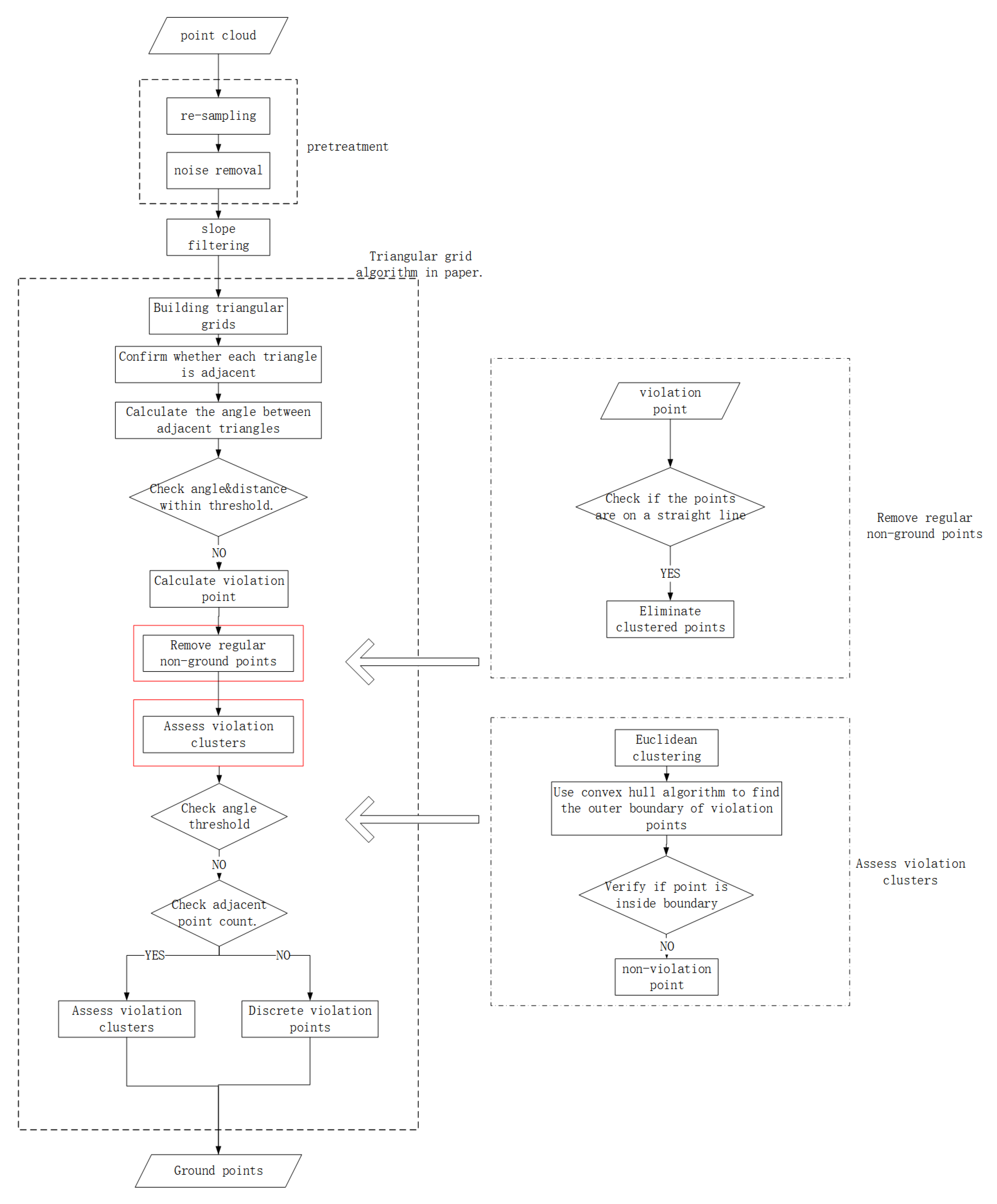
Figure 2.
How to obtain elevation grid.
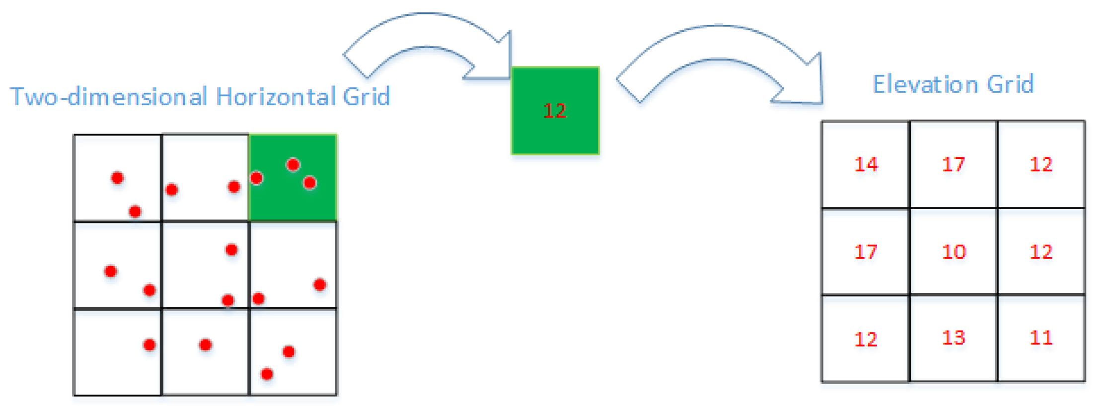
Figure 3.
How to obtain slope grid.
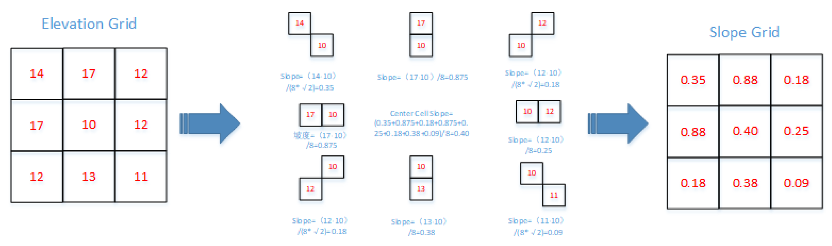
Figure 4.
How to obtain attribute grid.
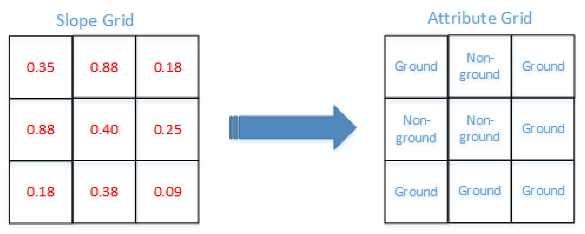
Figure 5.
Triangular grid.
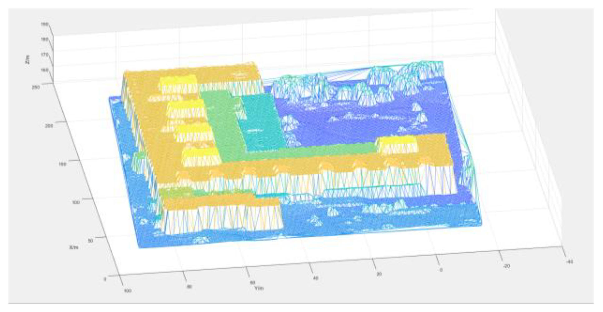
Figure 6.
The Euclidean Clustering.

Figure 7.
The Euclidean Clustering process.
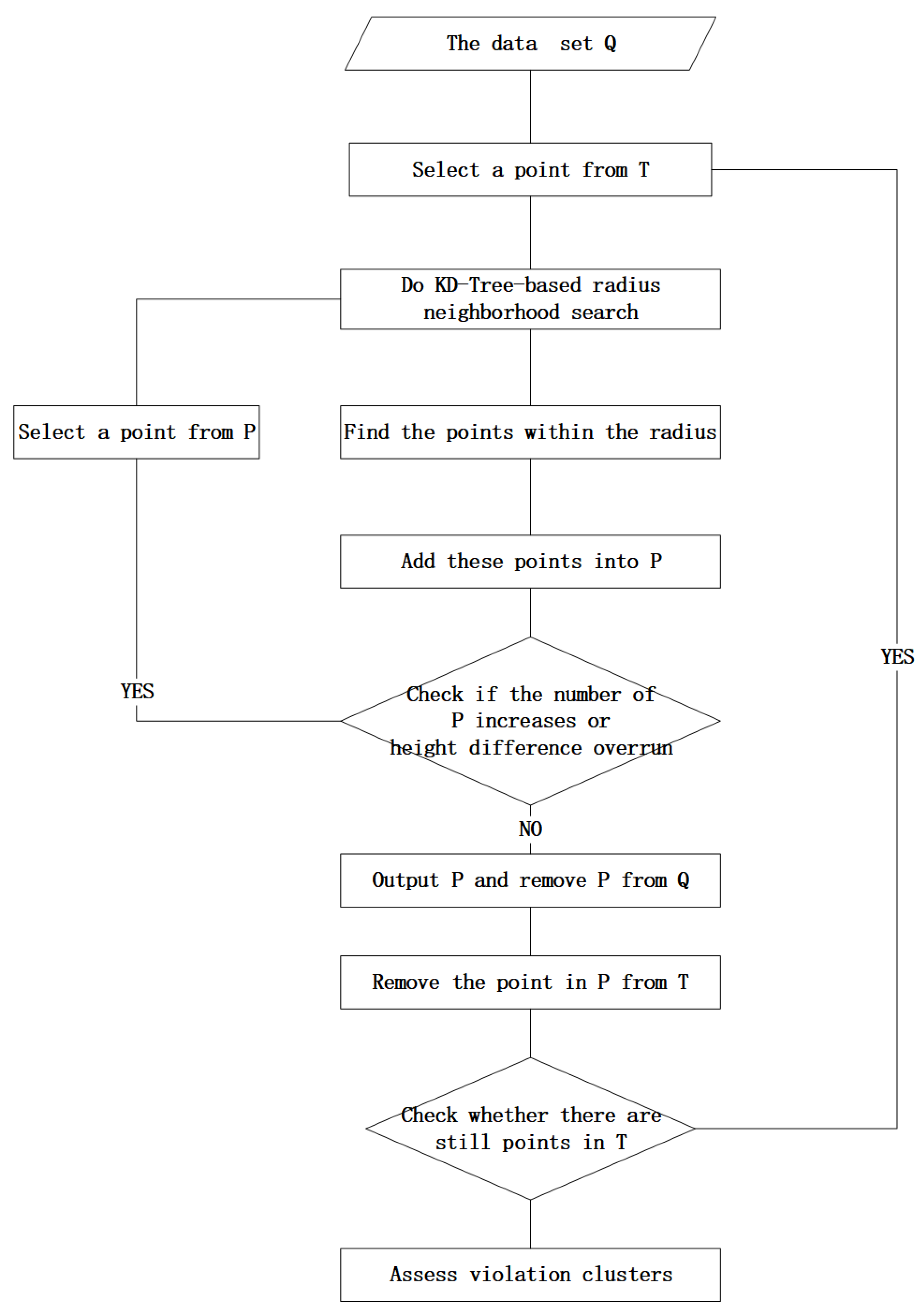
Figure 8.
The whole study point cloud.
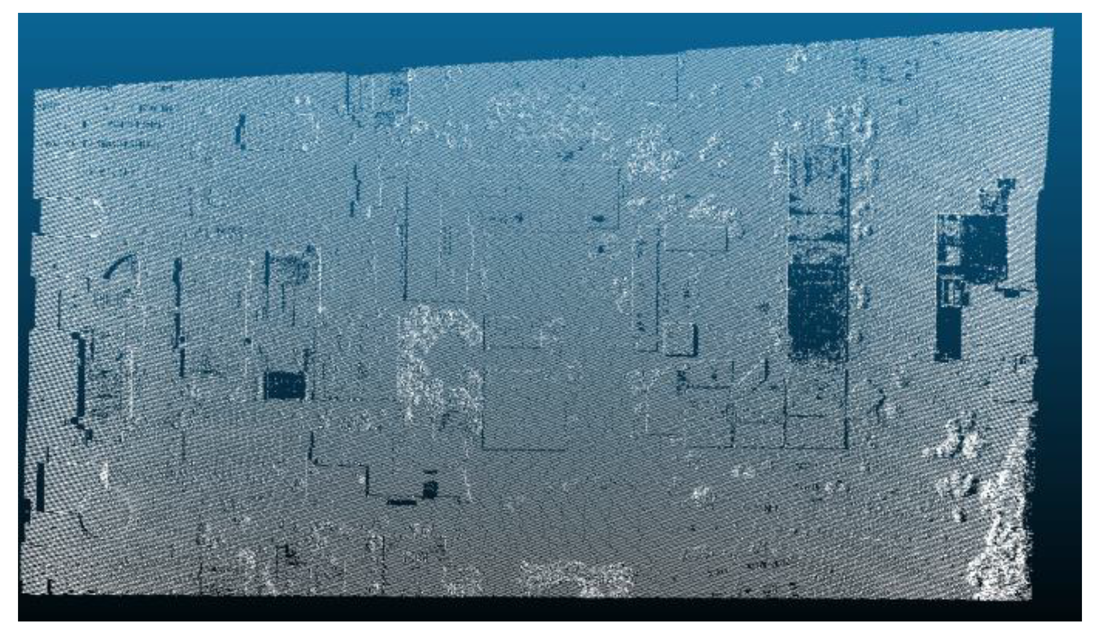
Figure 9.
The study area point cloud.
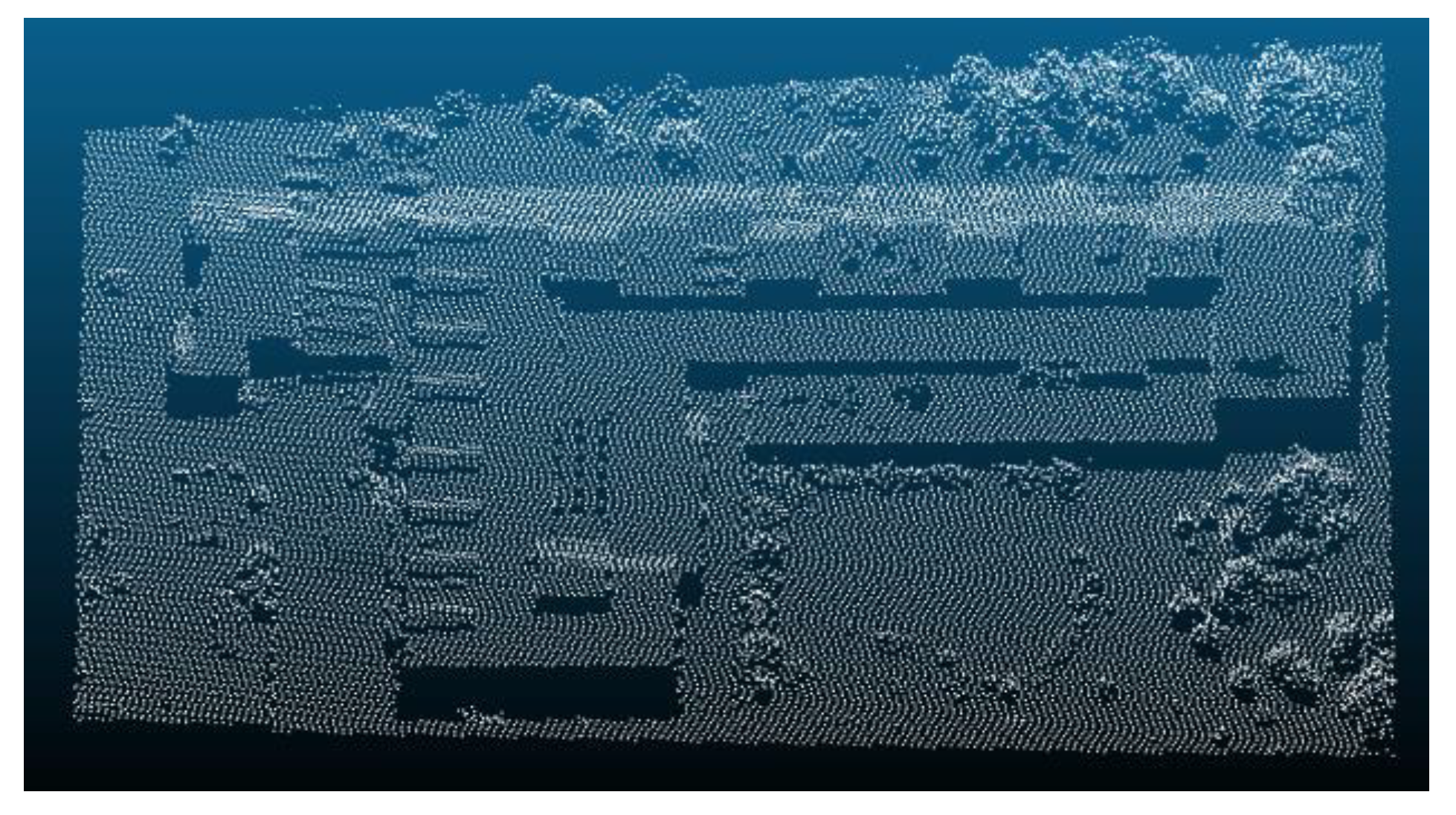
Figure 10.
The violation points.
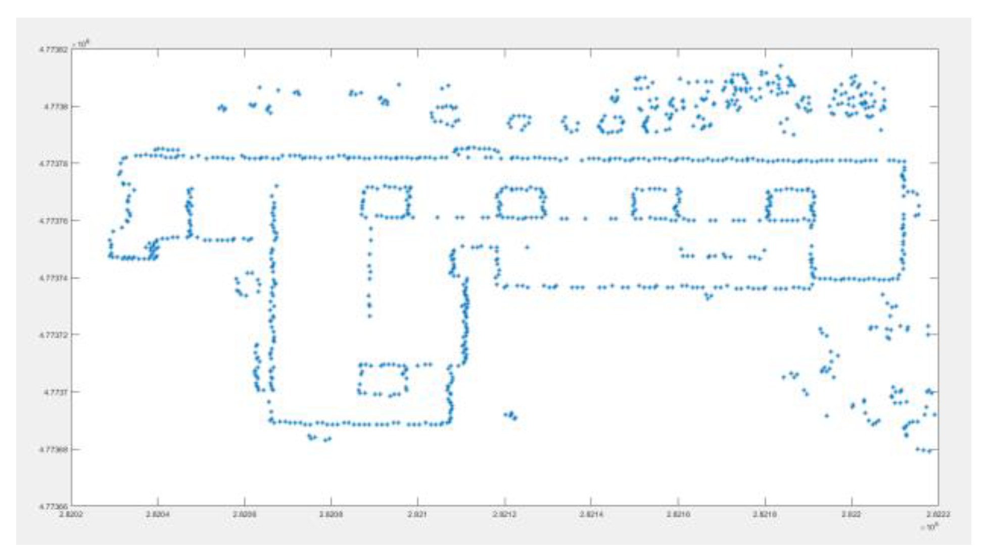
Figure 11.
The regular violation point.
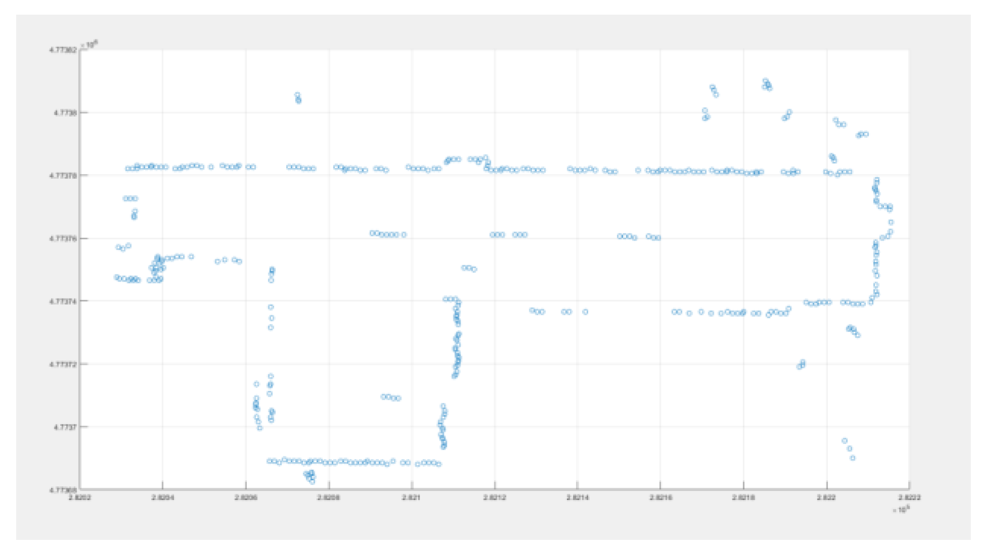
Figure 12.
The clustering result.
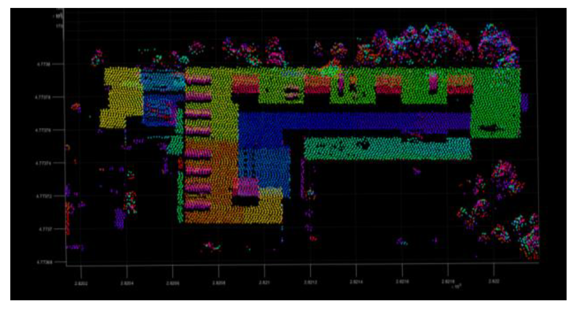
Figure 13.
The boundry of the clustering points.
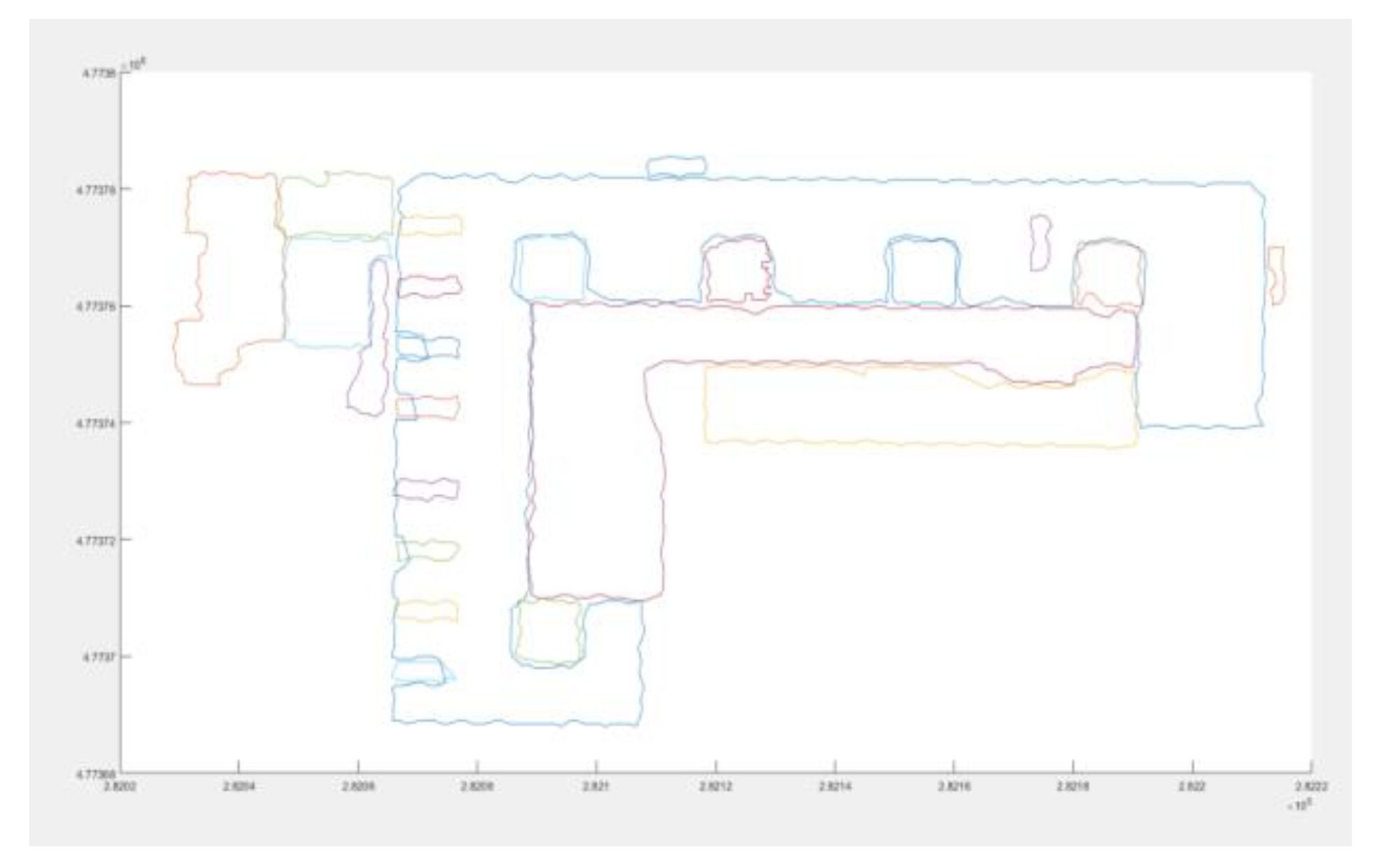
Figure 14.
The violation points of second round.
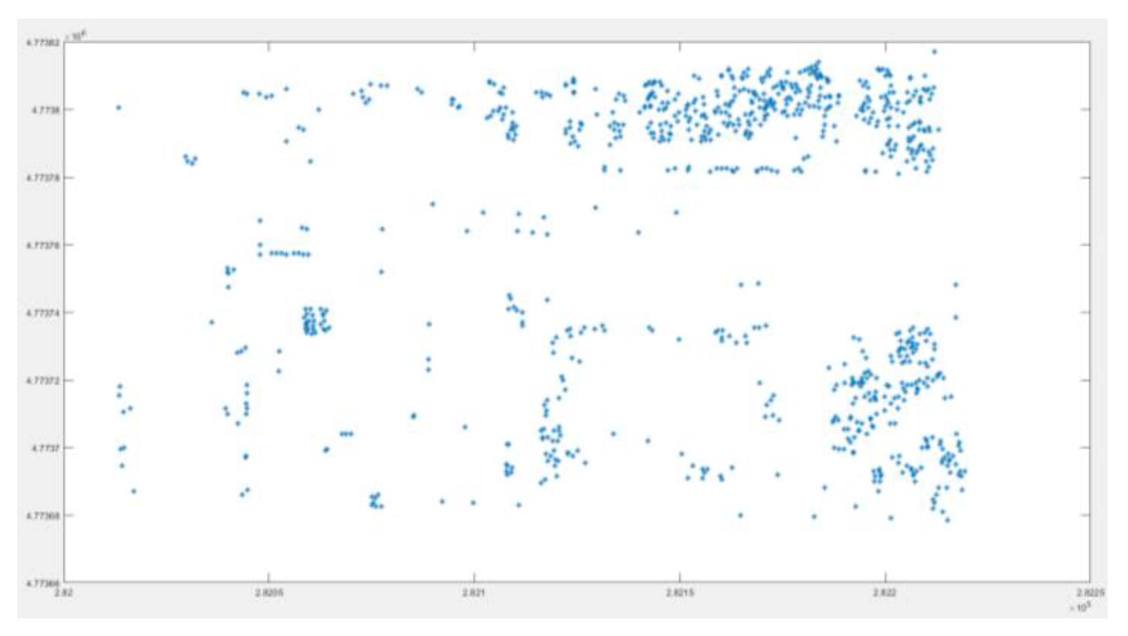
Figure 15.
The Study area after Triangular Grid Filter.
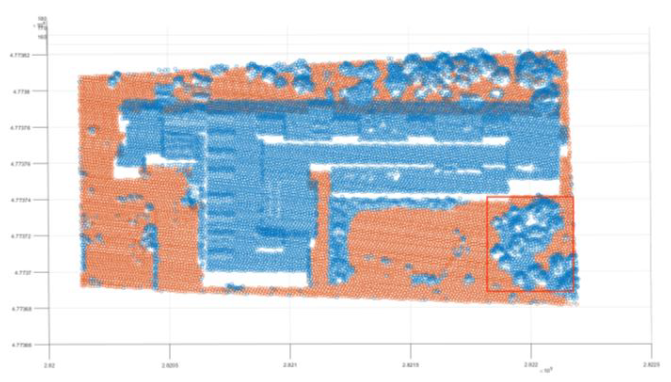
Figure 16.
The study area after Slope Filter with high threshold.
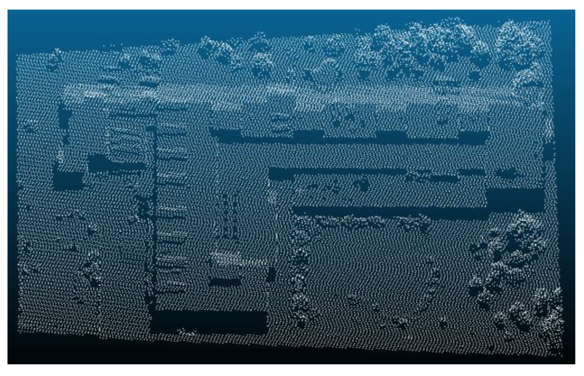
Figure 17.
The study area after filter combining two methods.
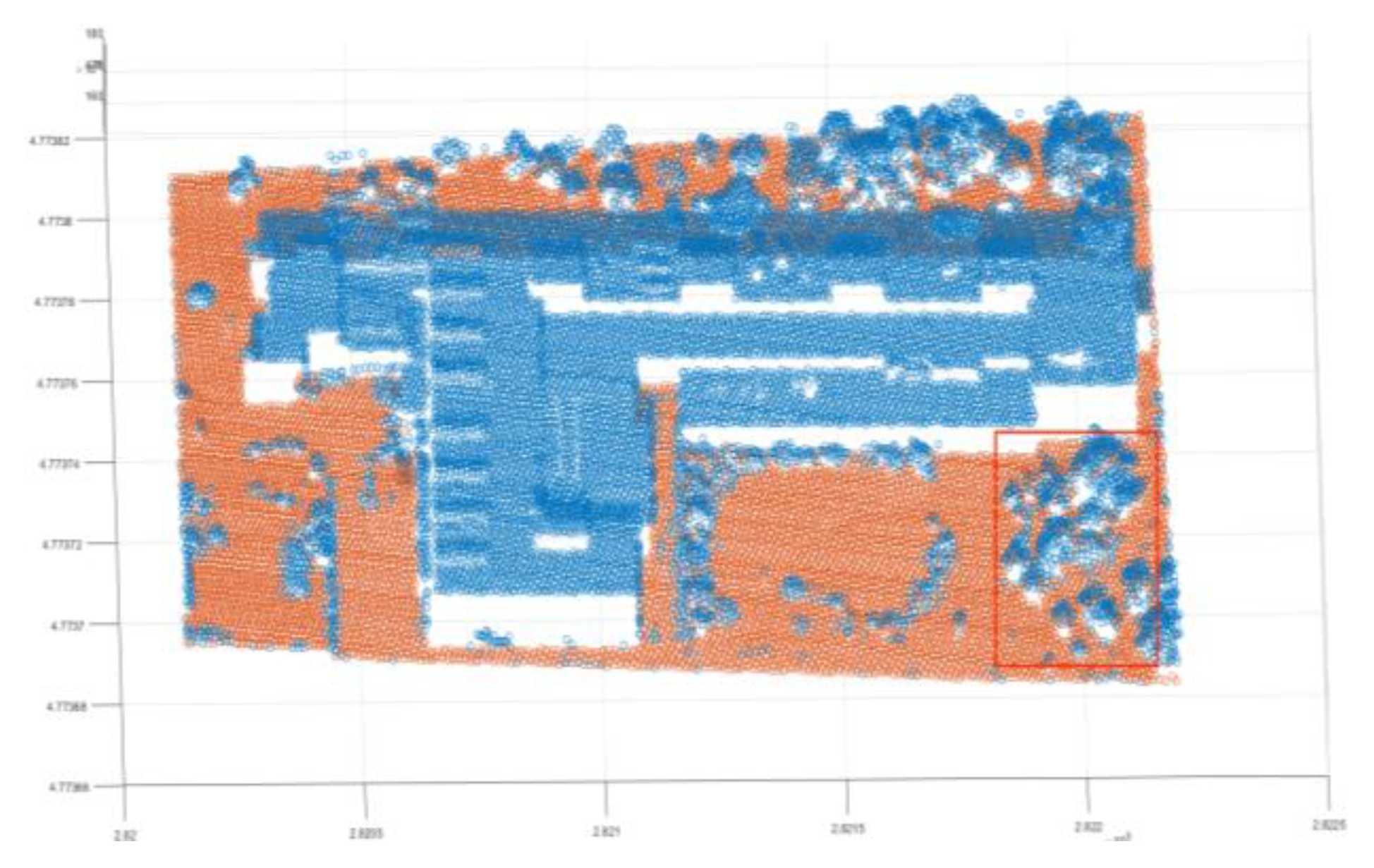
Figure 18.
EMD Filter.
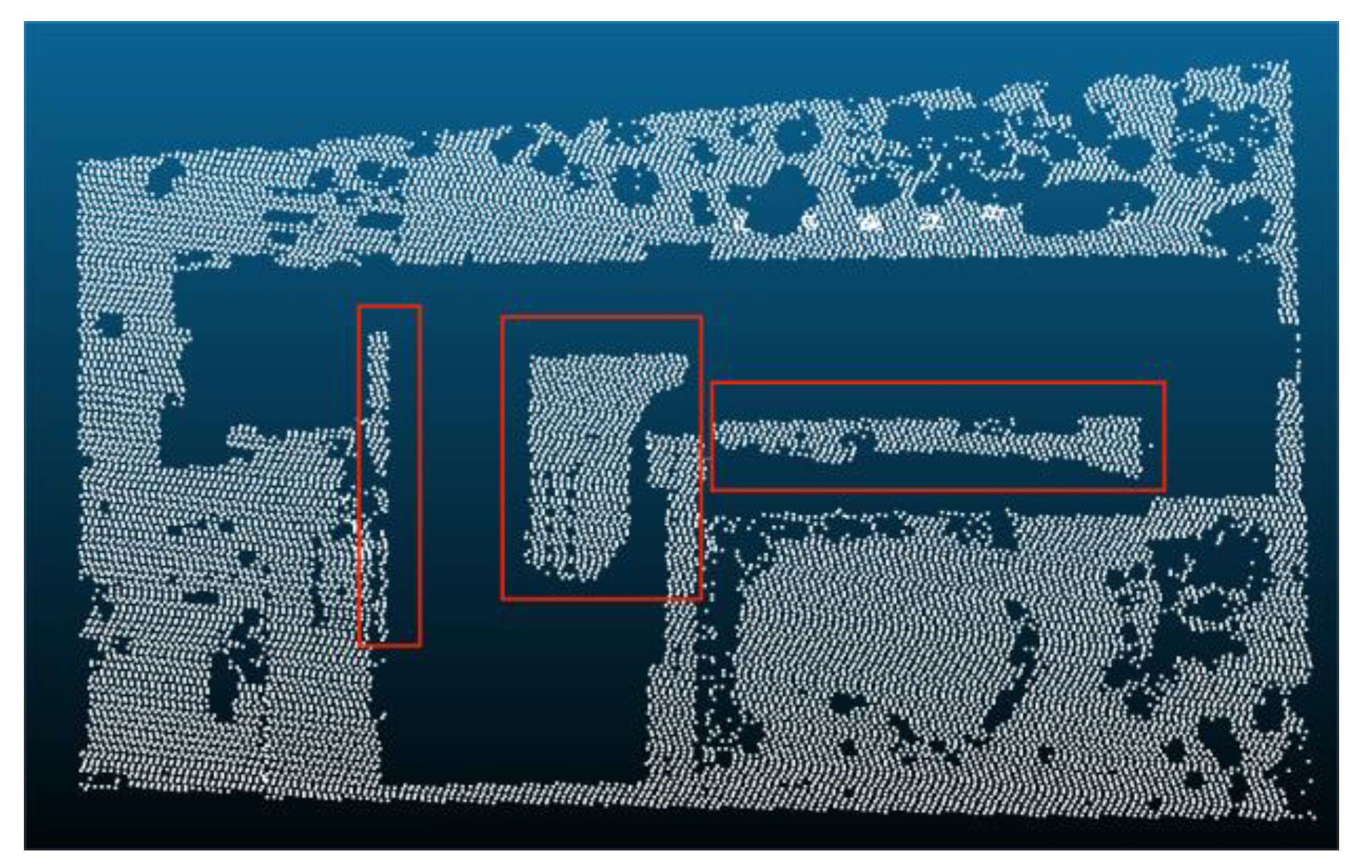
Figure 19.
SMRF Filter.
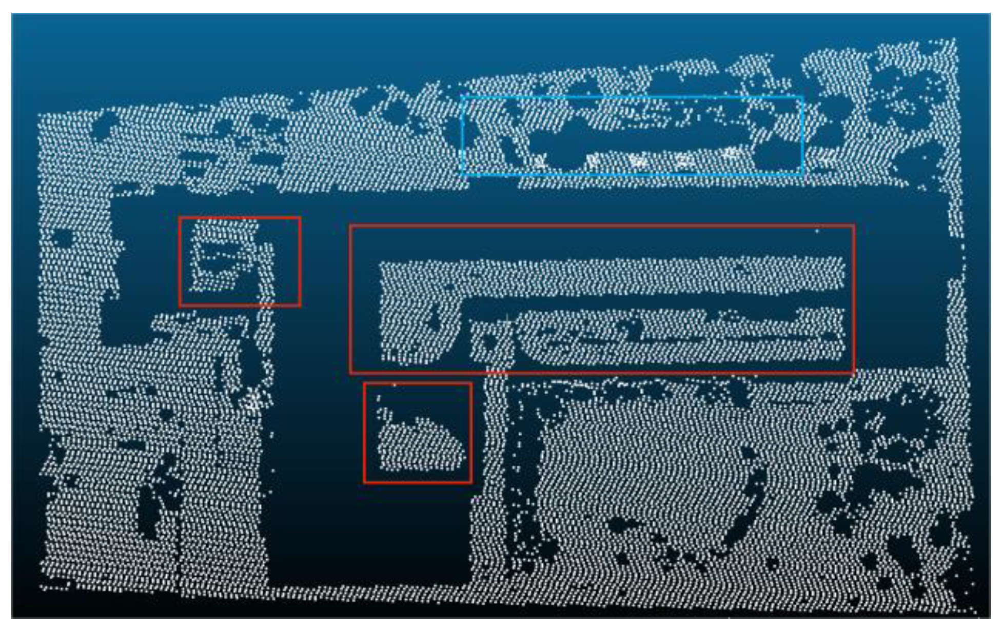
Figure 20.
Progressive Triangular Mesh Filter.

Figure 21.
Slope Filter.
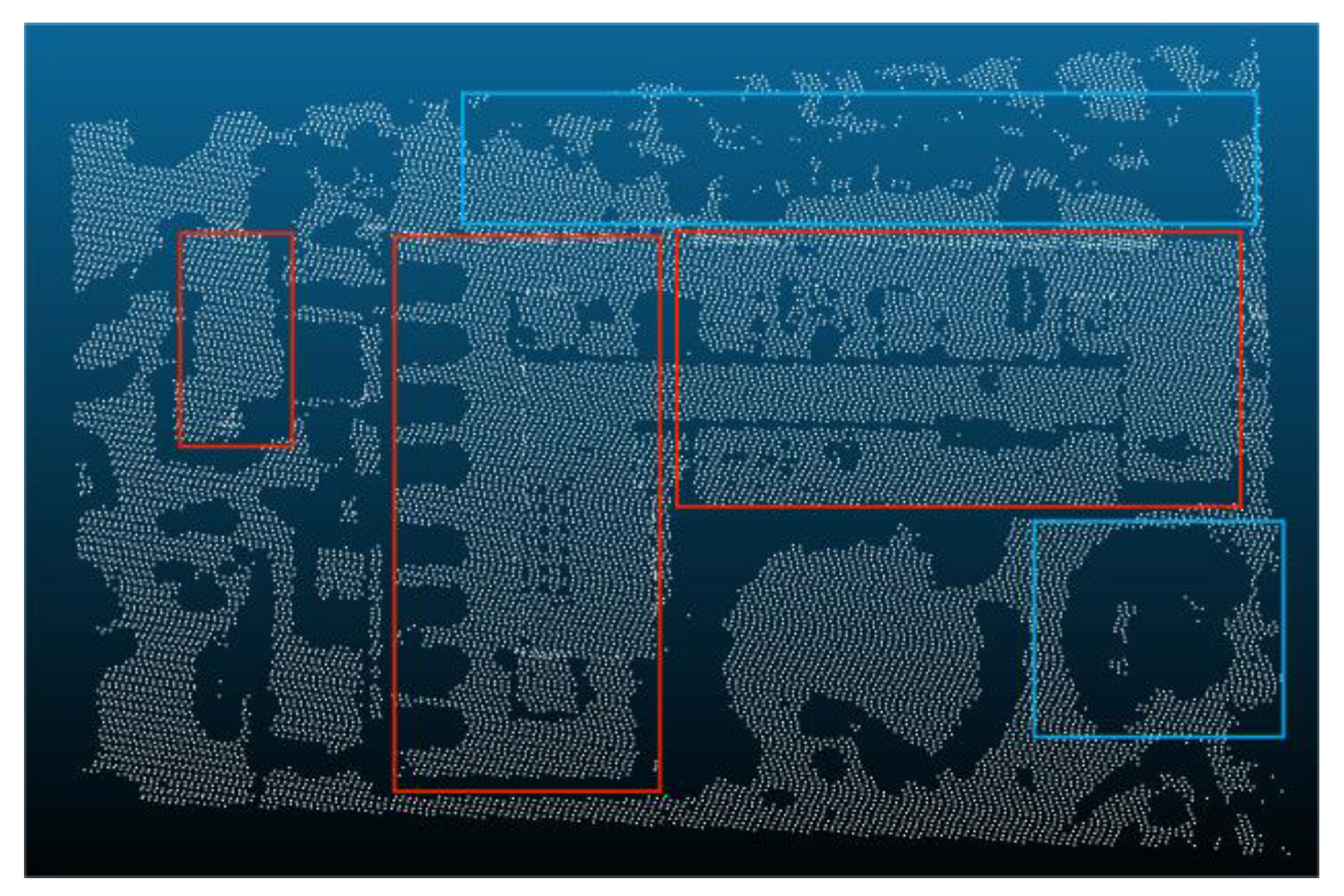
Figure 22.
Cloth Simulation Filter.
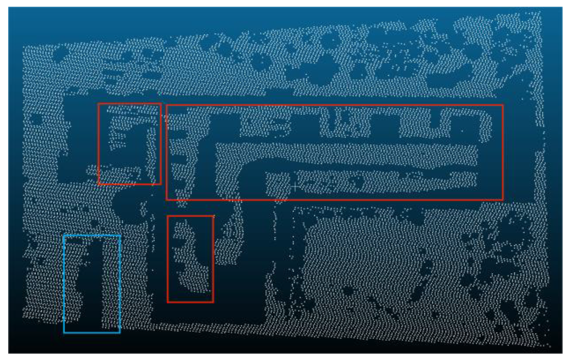
Figure 23.
Combining Slope Filter and Triangular Grid Filter.
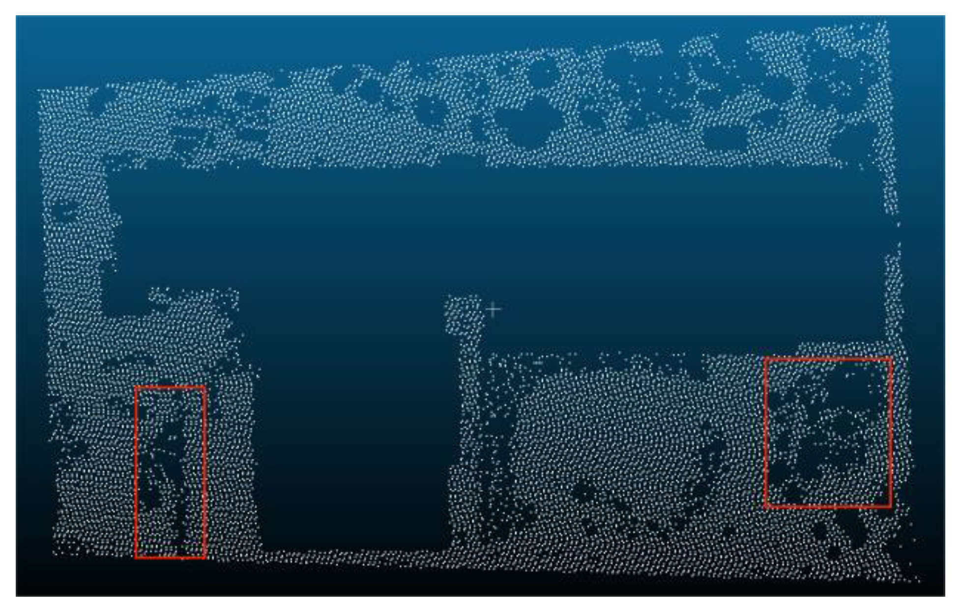
Figure 24.
Sample 1-1 after filter.
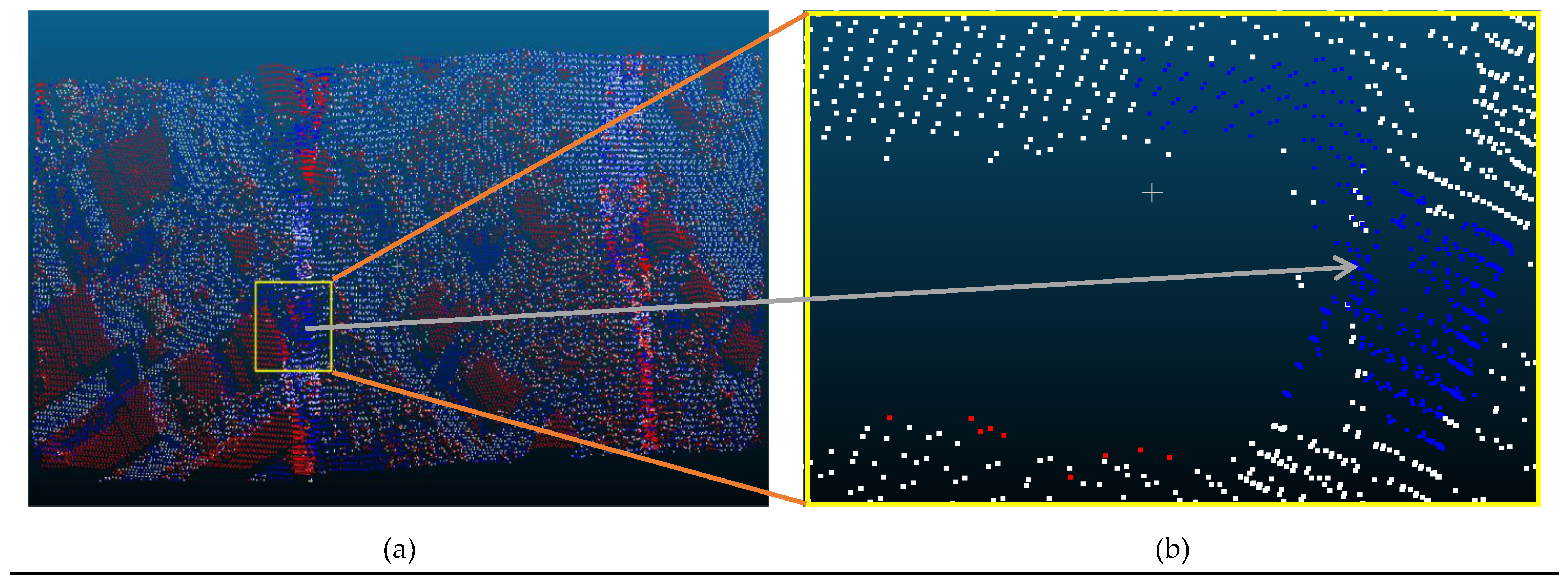
Figure 25.
Sample 1-2 after filter.
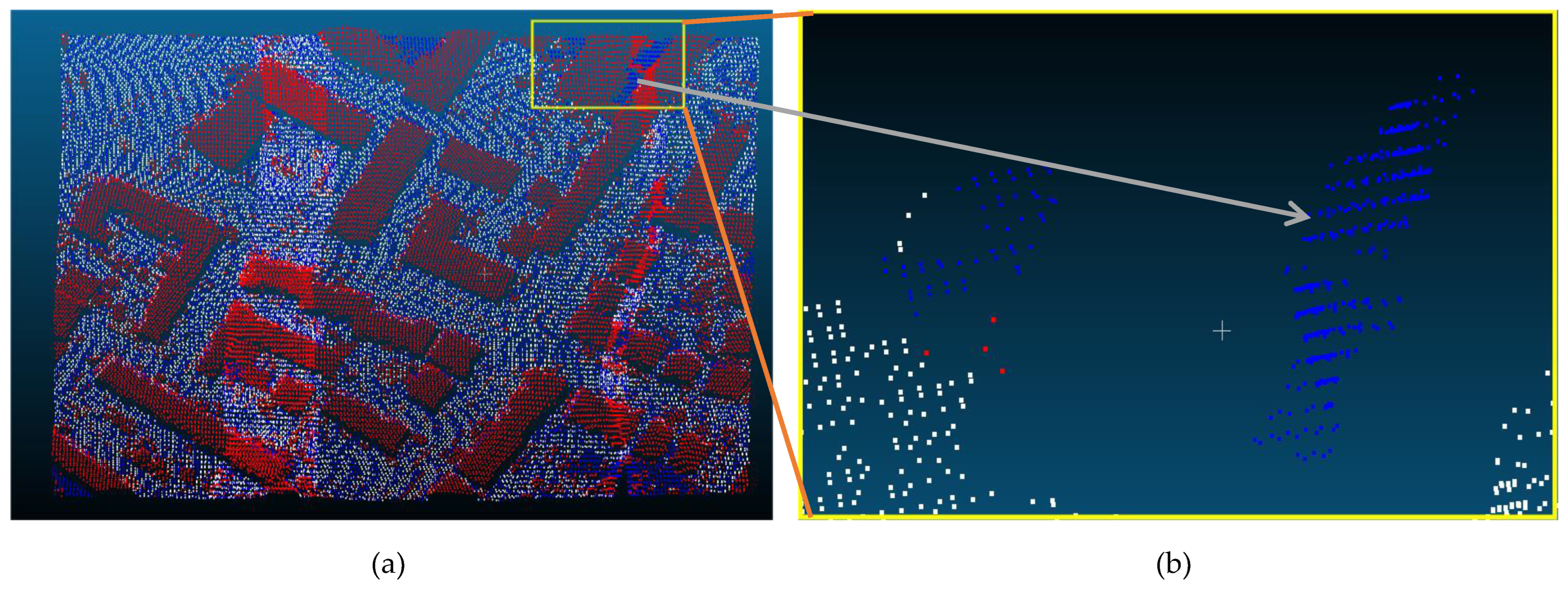
Figure 26.
Sample 2-1 after filter.
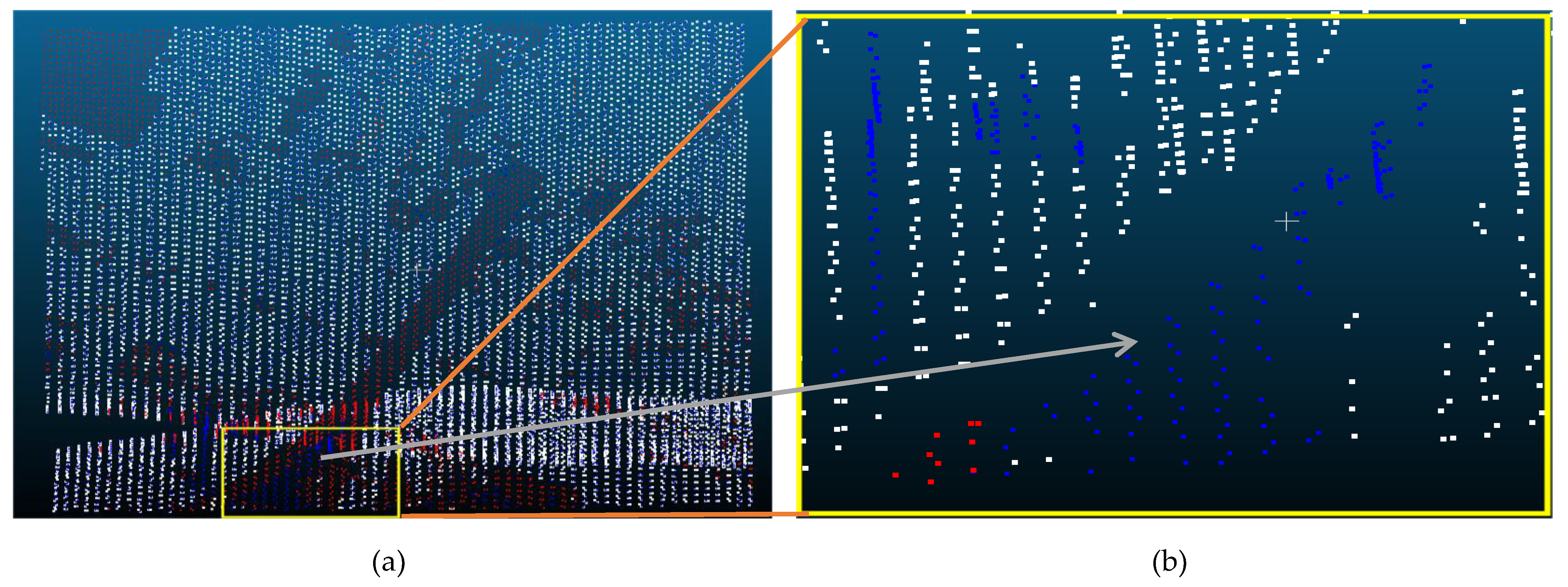
Figure 27.
Sample 2-2 after filter.
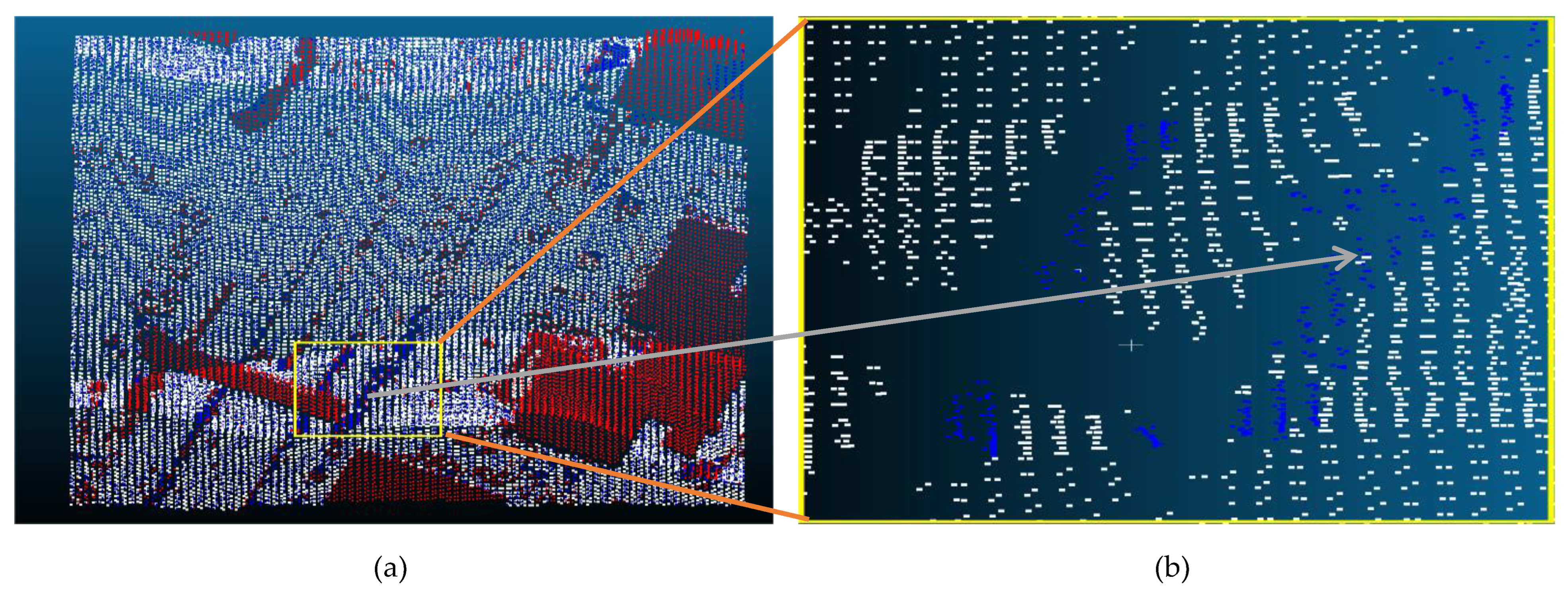
Figure 28.
Sample 2-3 after filter.
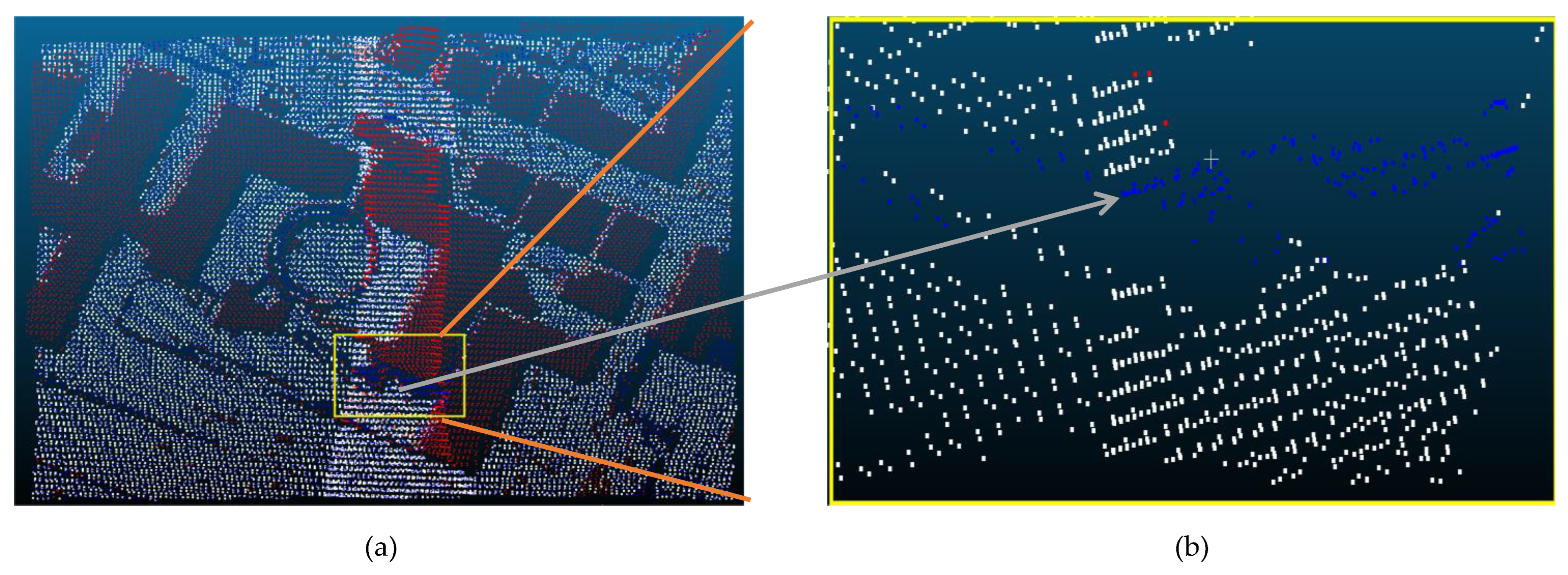
Figure 29.
Sample 2-4 after filter.
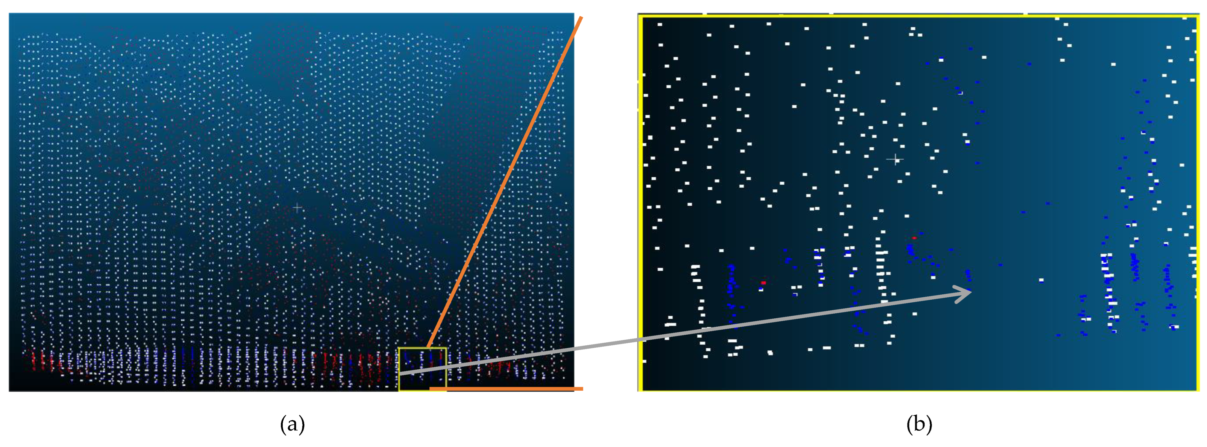
Figure 30.
Sample 3-1 after filter.
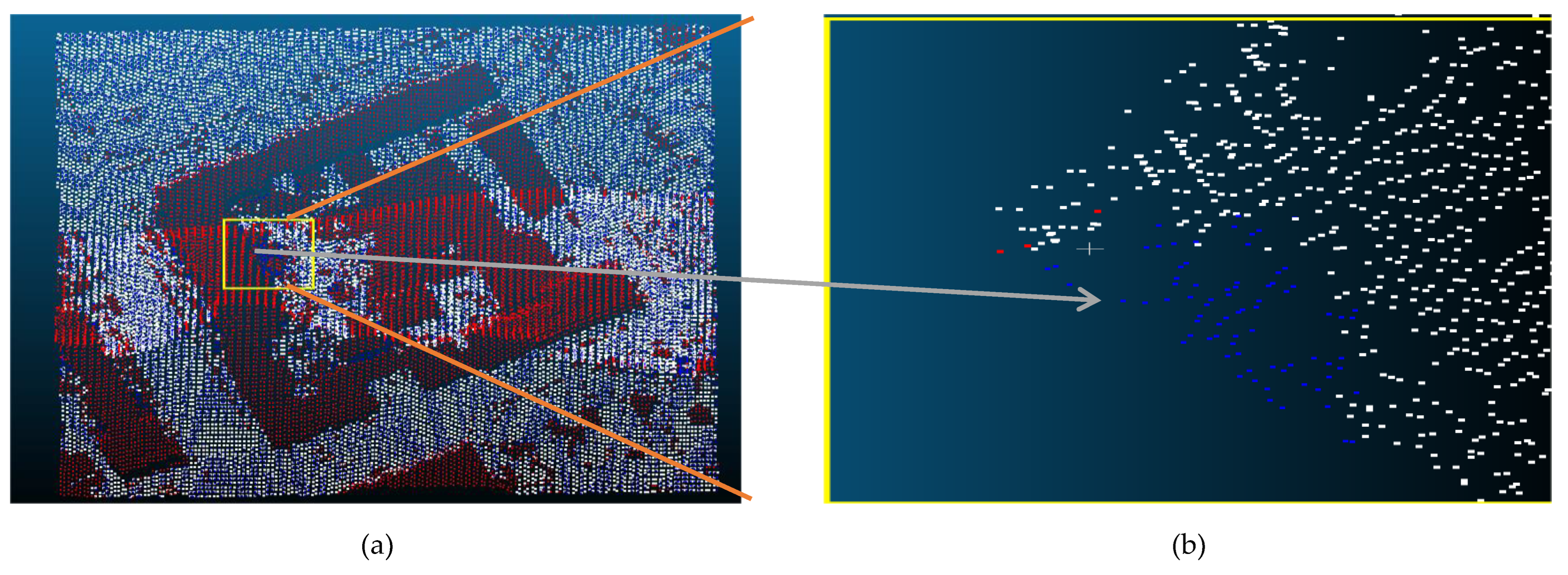
Figure 31.
Sample 4-1 after filter.

Figure 32.
Sample 4-2 after filter.
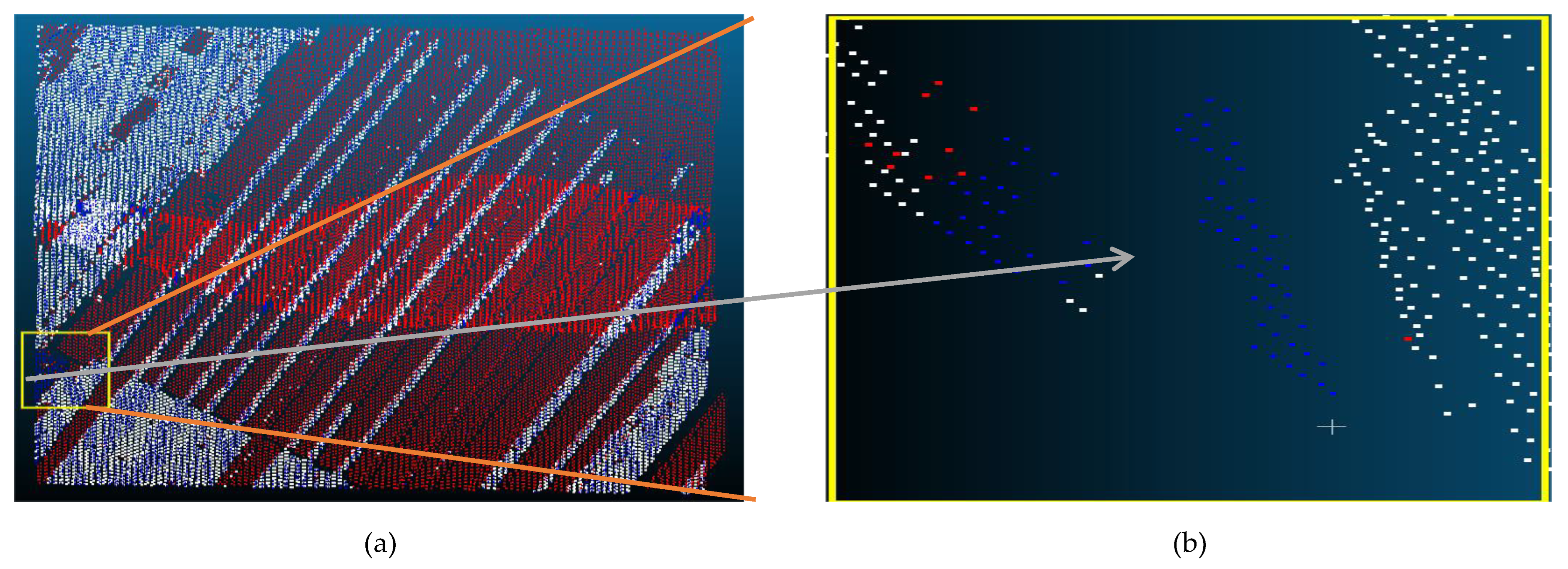
Figure 33.
Sample 5-1 after filter.
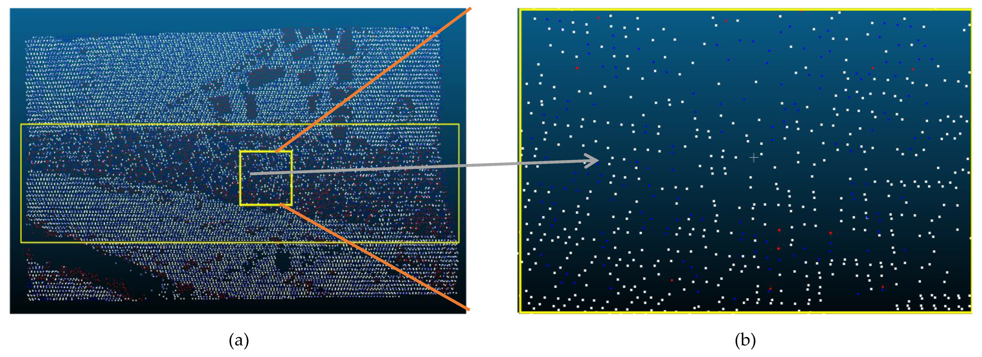
Figure 34.
Sample 5-2 after filter.
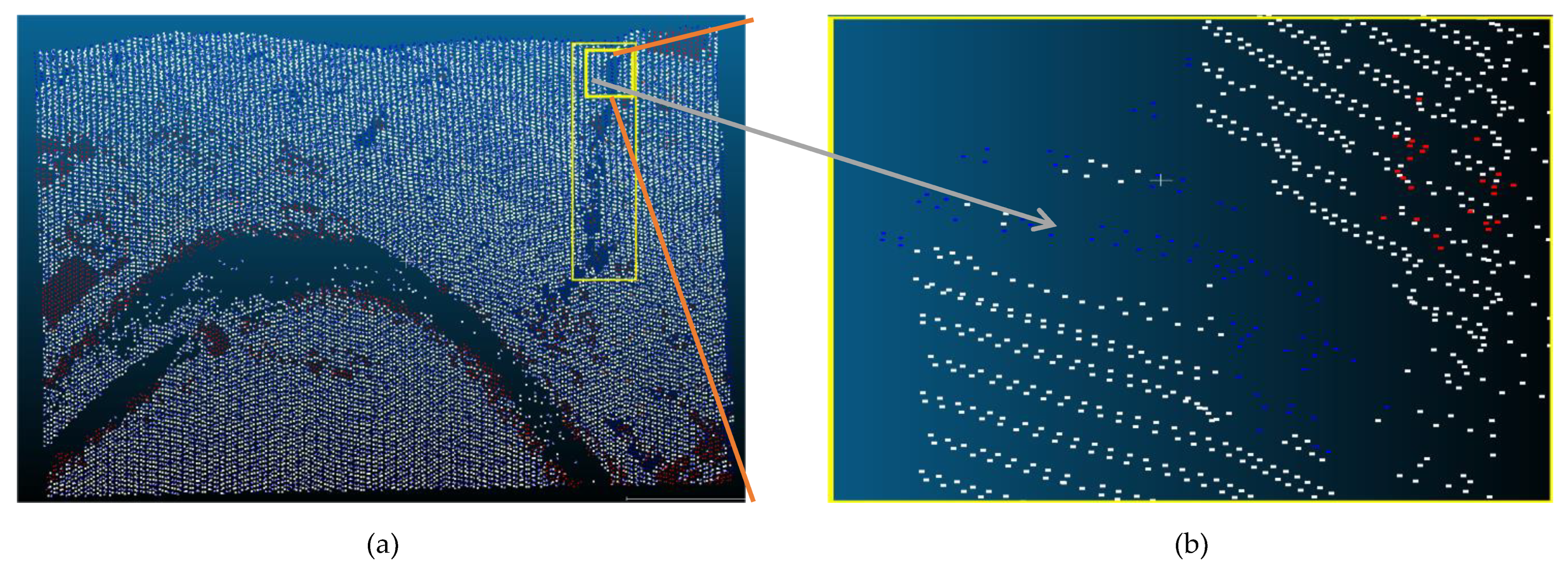
Figure 35.
Sample 5-3 after filter.
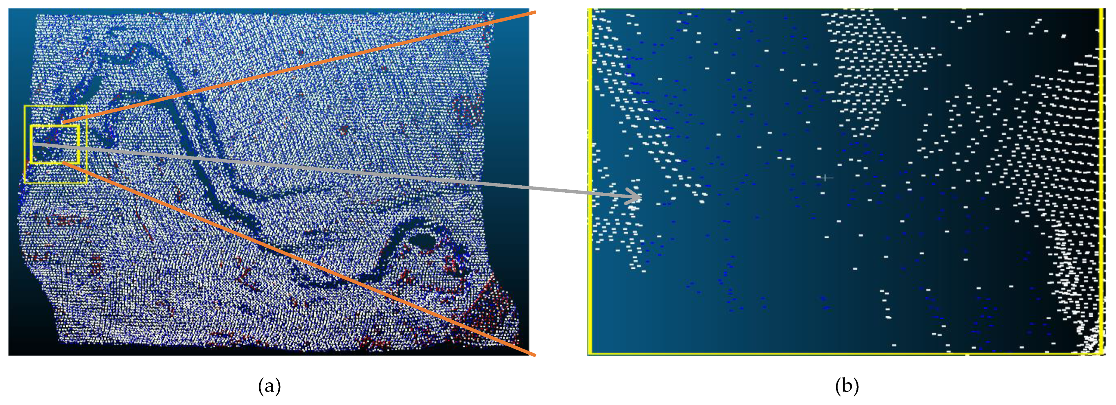
Figure 36.
Sample 5-4 after filter.
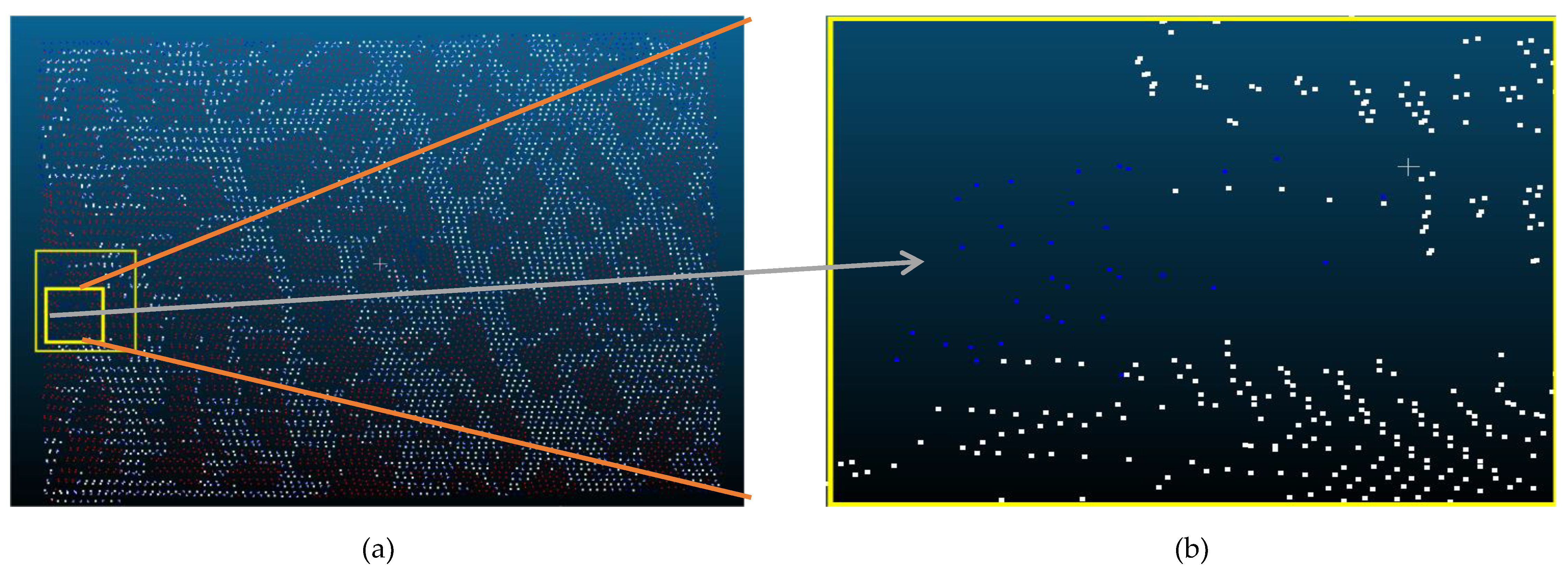
Figure 37.
Sample 6-1 after filter.
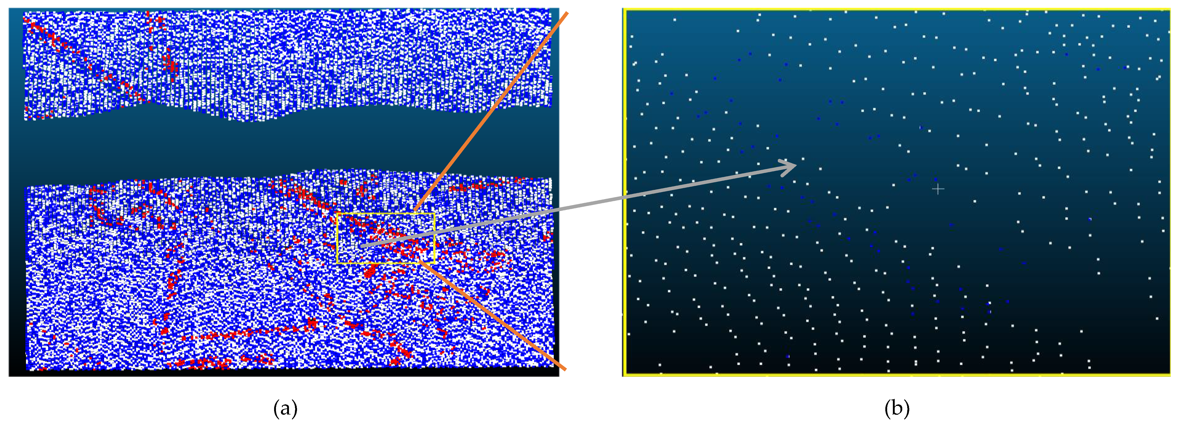
Figure 38.
Sample 7-1 after filter.
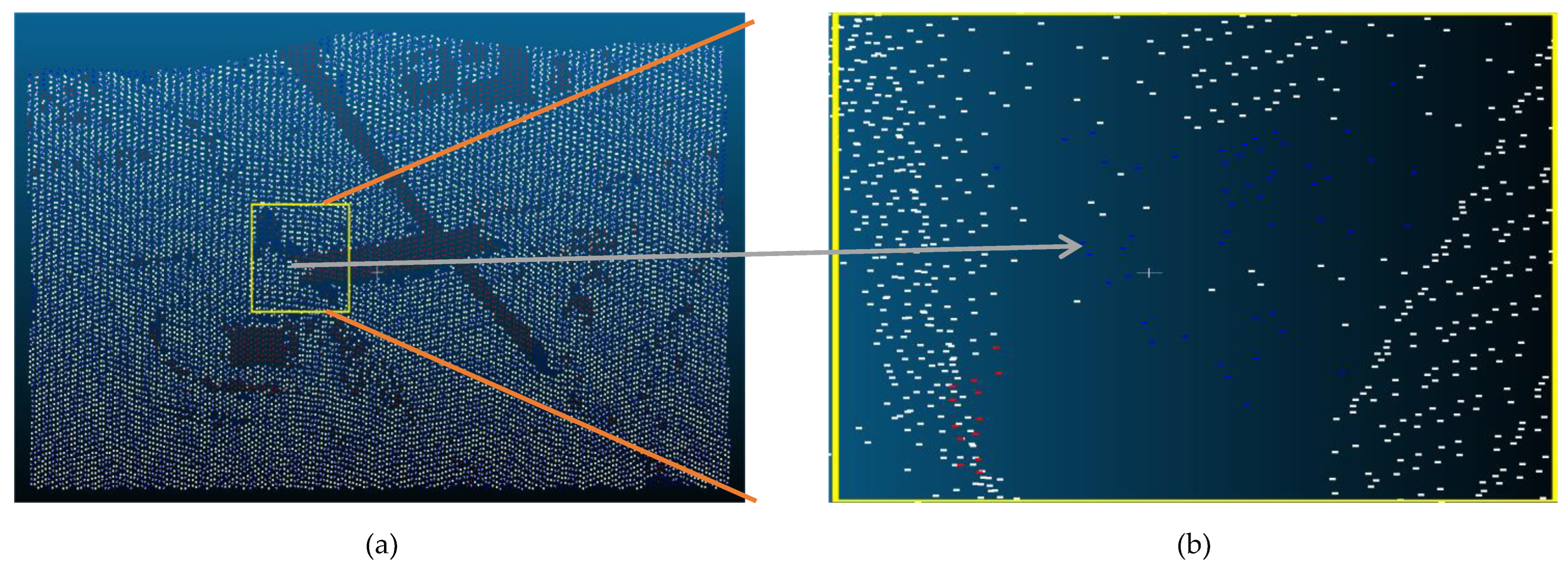
Figure 39.
The error of different methods in each sample.
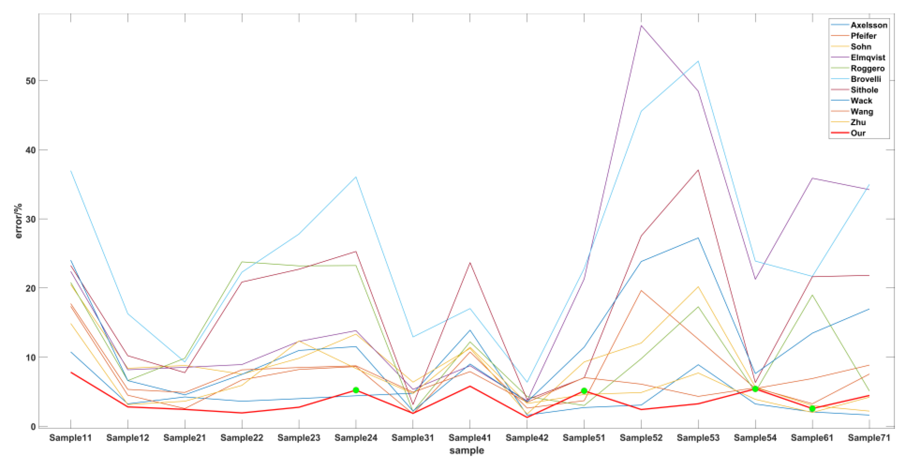
Figure 40.
Sample 3-1 surface reconstruction.
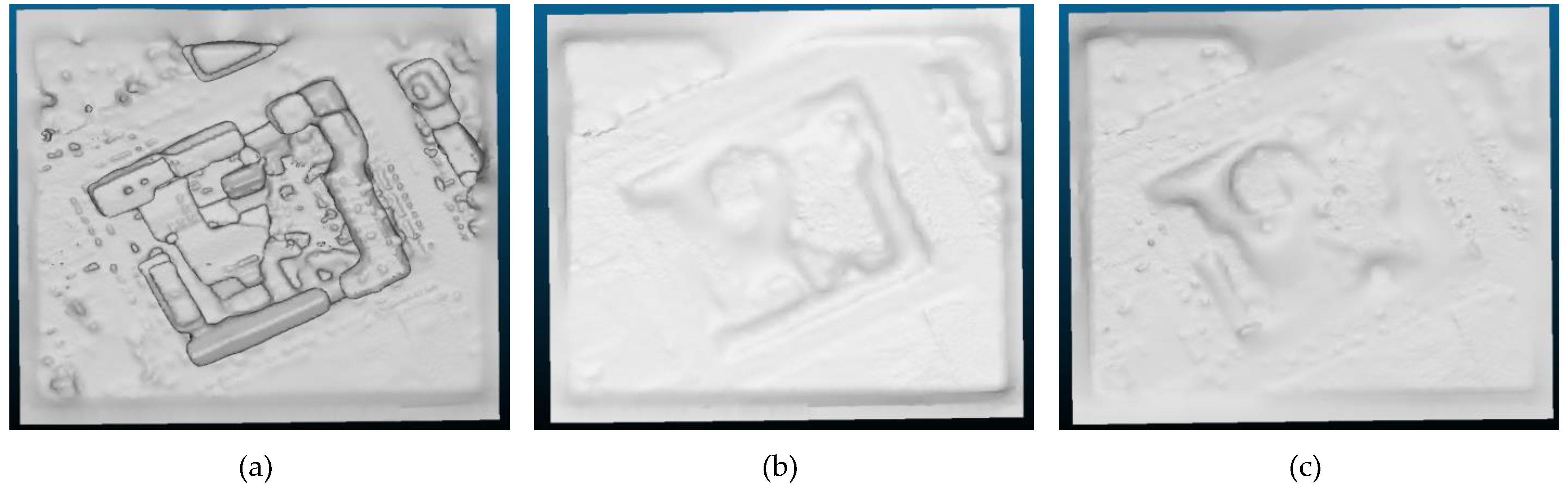
Figure 41.
Sample 5-4 surface reconstruction.
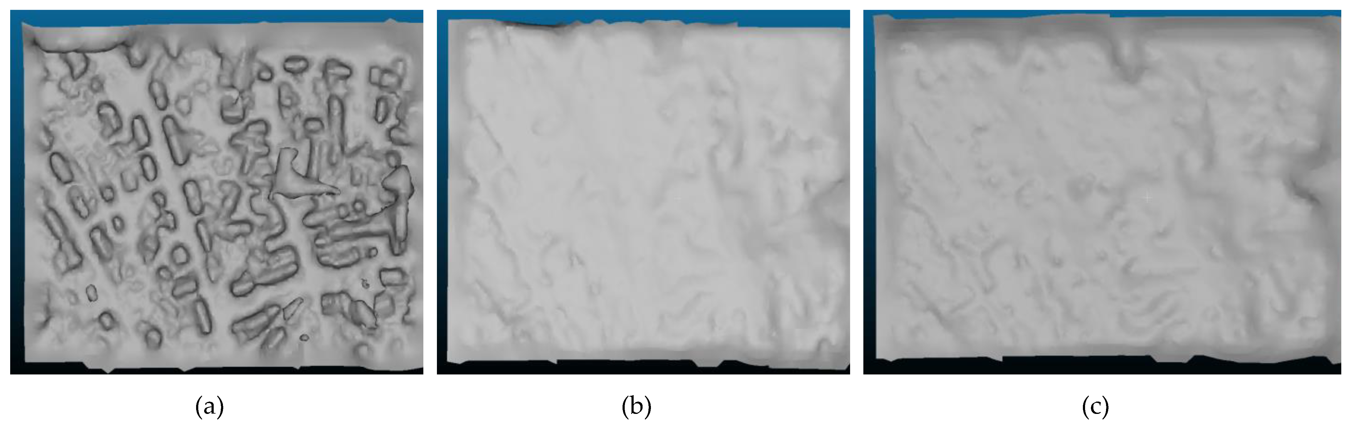

Table 1.
Filter Error Definition.
| Reference Data | Filtered data | Reference Data | |
| The point of ground | The point of non-ground | ||
| The point of ground | a | b | e = a + b |
| The point of non-ground | c | d | f = c + d |
| The point after Filter | g = a + c | h = b + d | n = a + b + c + d |
Table 2.
Three Type errors of Different Methods(%).
| Filter approach | Type I error | Type II error | Total Error |
|---|---|---|---|
| EMD Filter[22] | 3. 5 | 33. 2 | 15. 4 |
| SMRF Filter[23] | 2. 4 | 35. 4 | 15. 8 |
| Segmentation-Based Filtering[5] | 1. 66 | 1. 64 | 1. 65 |
| Slope Filter[7] | 8. 5 | 23. 8 | 14. 7 |
| Cloth Simulation Filter[6] | 4. 57 | 2. 61 | 3. 77 |
| Our | 0. 76 | 0. 39 | 0. 55 |
Table 3.
Three Type errors of Different Samples(%).
| Sample | Type I error | Type II error | Total Error |
|---|---|---|---|
| 1-1 | 10.76 | 3.86 | 7. 82 |
| 1-2 | 4.68 | 2.32 | 2. 81 |
| 2-1 | 2.70 | 1.57 | 2. 45 |
| 2-2 | 2.10 | 0. 72 | 1. 94 |
| 2-3 | 3.32 | 2.14 | 2. 76 |
| 2-4 | 5.26 | 5.15 | 5. 23 |
| 3-1 | 1.90 | 1.87 | 1. 88 |
| 4-1 | 10.64 | 0. 98 | 5. 80 |
| 4-2 | 3.76 | 0.26 | 1. 29 |
| 5-1 | 5.74 | 2.93 | 5. 13 |
| 5-2 | 2.14 | 4.91 | 2. 43 |
| 5-3 | 2.41 | 23. 47 | 3. 26 |
| 5-4 | 5.72 | 5.15 | 5. 41 |
| 6-1 | 1.05 | 31.76 | 2. 57 |
| 7-1 | 1.77 | 25.59 | 4. 46 |
| average | 4.26 | 7.51 | 3. 68 |
Table 4.
The Total Error Of Different Methods(%).
| Site | Sample | Axelsson [5] |
Pfeifer [24] |
Sohn [25] |
Elmqvist [26] |
Roggero [27] |
Brovelli [28] |
Sithole [2] |
Wack [29] |
Wang [9] |
Zhu [8] |
Our |
|---|---|---|---|---|---|---|---|---|---|---|---|---|
| Urban | 1-1 | 10. 76 | 17. 35 | 20. 49 | 22. 40 | 20. 80 | 36. 96 | 23. 25 | 24. 02 | 17. 74 | 14. 87 | 7. 82 |
| 1-2 | 3. 25 | 4. 50 | 8. 39 | 8. 18 | 6. 61 | 16. 28 | 10. 21 | 6. 61 | 5. 34 | 3. 14 | 2. 81 | |
| 2-1 | 4. 25 | 2. 57 | 8. 8 | 8. 53 | 9. 84 | 9. 30 | 7. 76 | 4. 55 | 4. 90 | 3. 63 | 2. 45 | |
| 2-2 | 3. 63 | 6. 71 | 7. 54 | 8. 93 | 23. 78 | 22. 28 | 20. 86 | 7. 51 | 8. 17 | 5. 92 | 1. 94 | |
| 2-3 | 4. 00 | 8. 22 | 9. 84 | 12. 28 | 23. 20 | 27. 80 | 22. 71 | 10. 97 | 8. 50 | 12. 34 | 2. 76 | |
| 2-4 | 4. 42 | 8. 64 | 13. 33 | 13. 83 | 23. 25 | 36. 06 | 25. 28 | 11. 53 | 8. 75 | 8. 36 | 5. 23 | |
| 3-1 | 4. 78 | 1. 80 | 6. 39 | 5. 34 | 2. 14 | 12. 92 | 3. 15 | 2. 21 | 4. 93 | 4. 74 | 1. 88 | |
| 4-1 | 13. 91 | 10. 75 | 11. 27 | 8. 76 | 12. 21 | 17. 03 | 23. 67 | 9. 01 | 7. 91 | 11. 44 | 5. 80 | |
| 4-2 | 1. 62 | 2. 64 | 1. 78 | 3. 68 | 4. 30 | 6. 38 | 3. 85 | 3. 54 | 3. 48 | 3. 30 | 1. 29 | |
| Rural | 5-1 | 2. 72 | 3. 71 | 9. 31 | 21. 31 | 3. 01 | 22. 81 | 7. 02 | 11. 45 | 7. 05 | 4. 61 | 5. 13 |
| 5-2 | 3. 07 | 19. 64 | 12. 04 | 57. 95 | 9. 78 | 45. 56 | 27. 53 | 23. 83 | 6. 10 | 4. 89 | 2. 43 | |
| 5-3 | 8. 91 | 12. 60 | 20. 19 | 48. 45 | 17. 29 | 52. 81 | 37. 07 | 27. 24 | 4. 33 | 7. 71 | 3. 26 | |
| 5-4 | 3. 23 | 5. 47 | 5. 68 | 21. 26 | 4. 96 | 23. 89 | 6. 33 | 7. 63 | 5. 57 | 3. 90 | 5. 41 | |
| 6-1 | 2. 08 | 6. 91 | 2. 99 | 35. 87 | 18. 99 | 21. 68 | 21. 63 | 13. 47 | 3. 26 | 2. 01 | 2. 57 | |
| 7-1 | 1. 63 | 8. 85 | 2. 20 | 34. 22 | 5. 11 | 34. 98 | 21. 83 | 16. 97 | 7. 56 | 4. 21 | 4. 46 | |
| average | 4. 82 | 8. 02 | 9. 35 | 20. 73 | 12. 34 | 25. 78 | 17. 48 | 12. 04 | 6. 91 | 6. 34 | 3. 68 | |
Disclaimer/Publisher’s Note: The statements, opinions and data contained in all publications are solely those of the individual author(s) and contributor(s) and not of MDPI and/or the editor(s). MDPI and/or the editor(s) disclaim responsibility for any injury to people or property resulting from any ideas, methods, instructions or products referred to in the content. |
© 2023 by the authors. Licensee MDPI, Basel, Switzerland. This article is an open access article distributed under the terms and conditions of the Creative Commons Attribution (CC BY) license (http://creativecommons.org/licenses/by/4.0/).
Copyright: This open access article is published under a Creative Commons CC BY 4.0 license, which permit the free download, distribution, and reuse, provided that the author and preprint are cited in any reuse.


