
Submitted:
02 May 2023
Posted:
03 May 2023
You are already at the latest version
Abstract
The influence of small-scale processes at the ocean-atmosphere boundary layer such as spray and foam on the surface waves prediction is studied. Estimates of the effect of including the exact number of specific fragmentation "parachute" type in the spray on the resulting drag coefficient is shown. For the estimates, the numerical simulations within WAVEWATCH III wave model are performed. The parameterizations of wind input were tested within WAVEWATCH III wave model: default ST4 and ST6 parameterizations and the ST1 and ST6 parameterizations used together with the implemented drag coefficient parameterization. The proposed parameterization takes into account the presence of foam and spay. The obtained results are compared with the NDBC buoys data. The importance of small-scale processes for waves at hurricane winds prediction and the prospects for their inclusion in modern numerical wave models is shown.
Keywords:
drag coefficient
; parameterizations
; wave model
; spray
; ocean-atmosphere boundary layer
1. Introduction
Numerical wave models based on the spectral representation of the wave distribution (WAVEWATCH III [1], SWAN [2], WAM [3]) generalize the main experimental and theoretical achievements obtained over the past years of the theory of surface waves [4]. In accordance with the increasing requirements for numerical forecasts, their spatial resolution is constantly increasing, however, increasing the spatial resolution in modern models of the circulation of the atmosphere and ocean requires, in turn, improving the quality of the description of the surface layer of the atmosphere, taking into account the heterogeneity of the underlying surface, which is determined by the sea state, the presence foam or ice, complex multi-phase composition of atmospheric air in strong winds, when wave breaking leads to the formation of spray. The construction of models of such complex phenomena must inevitably be based on experimental studies. In this case, the greatest difficulty is to take into account small-scale processes near the interfaces between atmosphere and hydrosphere, which, in principle, cannot be resolved in global numerical models and are specified in parametric dependencies using the so-called bulk formulas. For the boundary layer of the atmosphere and the hydrosphere, typical examples here are the effects associated with the waves breaking, the formation of spray, foam bubbles, which is especially important in the case of high wind speeds and hurricane conditions. To date, the average intensity of emerging storms is increasing due to climate change [5]. Hurricanes are accompanied by strong winds that create large waves that are dangerous for coastal areas in terms of flooding and possible erosion of the coastline. At the same time, high-precision forecasts of the weather and the sea surface will ensure the safety of the population and minimize losses from such natural phenomena.
Taking into account the designated importance of small-scale processes in extreme weather events (storms and hurricanes), their detailed studies have recently been carried out in the framework of laboratory modeling on experimental stands. The obtained results demonstrated the great influence of marine aerosol on the Earth system, including the physics and chemistry of the atmosphere above the oceans, and marine geochemistry and biogeochemistry in general [6,7]. It affects atmospheric transparency, remote sensing and air quality. The effect of sea spray can be considered as a plausible reason for the decrease in the surface drag coefficient in hurricane-force winds. The corresponding decrease in turbulent stress is explained in [8] by the exchange of momentum between the droplets and the air flow.
In this paper, we make the estimates of the parameters of exchange processes at the boundary between the ocean and the atmosphere under hurricane conditions based on the numerical prediction of surface waves. This took into account the effect that was recently named the main mechanism for the formation of spray in strong winds, fragmentation of the "parachute" type (see [9,10,11]). The proposed parameterization was subsequently tested taking into account small-scale processes in the WAVEWATCH III (WW3) wave model.
2. Methods
WW3 is based on the numerical solution of the equation for the spectral density of wave action N in the approximation of phase averaging:
The left hand side of the equation (1) describes the kinematics of waves, σ is the radian frequency, k is the wavenumber, θ is the wave direction. In the right hand side, there are terms that describe the wind input Sin, dissipation mainly due to wave breaking Sdis, and 4-wave nonlinear interaction of waves Snl. The model can take into account the processes of wave attenuation due to bottom friction, three-wave interaction in shallow water, energy dissipation on bottom inhomogeneities, the influence of currents, tides, the presence of subgrid-scale islands and ice cover.
In this paper, we focus on the Sin source term and its influence on the resulting wave parameters. In general, wind wave growth Sin is described by Miles mechanism and is given as wave growth under wind input as follows [12]:
here β is wind wave growth rate [12], it expresses wave growth by the wind input:
here с is phase velocity of the wave. β coefficient depends on friction velocity u*, which is formulated by the turbulent momentum flux:
here is air density, - fluctuation components of wind speed.
Experimental measurement of the magnitude of the turbulent momentum flux is a difficult task. One of the most common methods is the gradient method. The gradient method uses a logarithmic law based on the Prandtl and Karman boundary layer theory for a flat plate: under conditions of neutral stratification in a layer of constant flows (where the turbulent momentum flux does not depend on height), the wind speed profile is close to logarithmic (see, for example, [13]):
Here is the Von Kàrmàn constant, z0 is the roughness parameter. By analogy with the resistance of a flat plate, the drag coefficient of the water surface is introduced, which relates the measured wind speed and the turbulent momentum flux (friction velocity):
where U10 is 10 m wind speed.
The parameterization of the CD drag coefficient is of great importance in momentum exchange in the atmospheric surface boundary layer especially at hurricane winds. Thus, to refine the wind input on waves at high (hurricane) wind speeds, it is necessary to use the parameterization of the drag coefficient, which takes into account additional effects that occur at such wind speeds, in particular, the influence of emerging spray and foam.
Wind input and dissipation in the WW3 wave model are represented by different parameterizations. The ST1 model (WAM 3) [14] is given by two empirical formulas. The first one is for the wind wave growth rate:
where Cin=0.25 is a constant parameter, is the relation of the air and water densities, θw is the mean wind direction, c is the phase velocity, N(k,θ) is the is the wave action density spectrum. The second one is the parameterization of the drag coefficient proposed in [15]:
This parameterization provides a relationship between the 10 m wind speed and friction velocity .
Here the omni-directional action density is obtained by integration over all directions:
The A(k) is the inverse directional spectral narrowness and is defined as:
for all directions .
The value of W takes into account the direction of the wind, considering W as the sum of the winds in the direction of the waves and the headwinds, so that they complement each other.
The drag coefficient is determined by the expression:
The parameterization was proposed in [19] and takes into account the saturation and further decrease in extreme winds of water resistance at wind speeds exceeding 30 m/s. To prevent u⋆ from dropping to zero in very strong winds (U10 ≥ 50.33 m/s), expression (18) was modified to give u⋆ = 2.026 m/s.
It should be noted that the parameterization ST6 also has a negative input term to attenuate wave growth in those parts of the wave spectrum where there is a negative component of wind stress (13), in addition to positive wind input. The growth rate for headwinds is negative [20].
ST4 [21] is also the modern widely used models of wind input. This parameterization is set iteratively, based on the WAM 4 model for the "positive contribution" of the wind, but introduces corrections that reduce the drag coefficient at high wind speeds. This is achieved by reducing the contribution of wind input at high winds.
3. Results and Discussion
3.1. Simulation
In this paper, a case of Irma hurricane is considered to test different parameterizations of wind input and drag coefficient parameterizations. It took place in 30/08/2017 - 12/09/2017 in the North Atlantic Ocean. Hurricane Irma was an extremely powerful Cape Verde hurricane. Irma developed from a tropical wave near Cape Verde on August 30, then it rapidly intensified into a Category 3 hurricane on the Saffir–Simpson wind scale on August 31. The intensity fluctuated on the next days, but on September 4, Irma resumed intensifying, becoming a Category 5 hurricane on the next day. The best track of the hurricane is made by USA National Hurricane Center and is shown on the Figure 1 taken from the tropical cyclone report [22]. The red dashed line shows the area that is considered in the simulation. NDBC buoys used for the further analysis are shown on the map by yellow points.
The numerical simulations of waves under hurricane Irma conditions are performed within WW3. The modelling covered the period of 01/09/2017 – 09/09/2017. The longitudes and latitudes of the considered area varied from 14 up to 24 degrees and from 280 up to 330 degrees respectively. The frequencies ranged in the interval from 0,037 Hz up to 2,97 Hz, 24 angular directions are considered. The ETOPO1 data is used to create bathymetry and mask files. The waves developed under wind forcing from the CFSv2 reanalysis with spatial resolution of 0,2050 [23]. It is necessary to mention, that in this test simulation the waves developed from the calm initial conditions and there are no waves in the considered area at the beginning of the simulation. The results are obtained after few hours from the beginning of the simulation. The simulations are carried out at the IAP RAS cluster using pure MPI option of the model code.
First, default approach is considered: two state-of-the-art parameterizations of wind input (ST4 [21] and ST6 [16,17]) are tested. The resulting significant wave height distribution is obtained for two types of wind input parameterizations: ST4 and ST6. The model reproduces the rotating and motion of the hurricane, and the asymmetry of the wave field distribution can be seen. On the Figure 2 the typical phases of a hurricane development and the increase of its intensification are shown. ST6 parameterization gives values higher than ST4 on approximately 15%. On September 6, the following hurricane Jose is also obtained.
3.2. Estimation of the air-sea exchange processes parameters
On the basis of the obtained in the simulations data, the parameters of exchange processes at the ocean - atmosphere boundary layer under hurricane conditions are estimated. Using the results of the wind and wave parameters obtained in the calculations, we estimated the surface drag coefficient and the effects associated with the formation of sea spray. The small-scale effect of "parachute" type fragmentation is taken into account [9,10,11]. The mechanism is the inflation and subsequent rupture of short-lived, sail-like elevations of the water surface. This process is similar to the “parachute” type fragmentation of liquid drops and jets in gas flows.
Based on the obtained data, a spray generation function is proposed for the parachute-type rupture mechanism, which depends on the wave fetch and satisfies both laboratory and field conditions, using the dimensionless Reynolds number (Re) [24]:
where u* is wind friction velocity, σp is peak frequency of surface waves, ν is the air kinematic viscosity. The function that best describes the experimental data is selected, it shows that the exact number of "parachutes" can be determined by the following equation (see Figure 3 a):
where M0=2.08, M1=972.
Taking into account the statistics of events associated with the formation of spray, the contribution of spray to the processes of exchange between the atmosphere and the ocean is estimated (see [11,25]). In particular, this makes it possible to explain the unusual nonmonotonic dependence of the sea surface drag coefficient on wind speed (see Figure 3b).
The curve in Figure 3b is obtained for a certain wave age parameter, defined as the ratio of the 10 m wind speed to the phase velocity of the waves corresponding to the peak in the frequency spectrum of surface waves c:
The surface drag coefficient is also estimated for the wave parameters calculated in the WW3 model for Hurricane Irma. On Figure 4 the examples of the distribution of parameters that determine the formation of spray and other exchange parameters associated with it are shown. Figure 4a shows the wind speed and direction distribution in Hurricane Irma according to the CFSv2 reanalysis. On Figure 4b, the frequency of the spectrum peak distribution calculated in the WW3 model is shown. On Figure 4c, the distribution of the surface drag coefficient estimated for the parameters in Figure 4 a, b, taking into account the contribution of sea spray and foam is shown. A decrease in the surface drag coefficient in the area of strong winds is demonstrated. The pronounced asymmetry of the distribution of surface drag coefficient in the direction of the storm center motion reflects the asymmetry of the surface wind and the wave distribution.
Thus, the estimates allow us to conclude that it is important to take into account the effect of spray and foam in the numerical simulation wave parameters. To take into account the effect of spray and foam in the parameterization of drag coefficient and, subsequently, in the wave model, it is convenient to obtain a formula expression for CD. Such an expression is obtained [30] in the framework of numerical experiments with the Lagrangian stochastic model (LSM), the drag coefficient depends on 10 m wind speed and wave age parameter and it is different for two ranges of wind speeds:
The feature of the obtained expression for CD includes the dependence not only on the wind speed, but also on the wave age, which is especially important at high wind speeds. Wave age varies in time and the values are completely different for the short waves that are in the beginning of the simulation (Ω=1 ÷ 1.5) to hurricane waves (Ω is up to 3) and then for the swell (Ω<1). On Figure 5 the change in the value of the wave age at one of the points in space where the hurricane passed is displayed. It can be seen that at first the wave age corresponds to the presence of short waves, however, from the moment the hurricane wind approaches, a sharp change in the peak frequency of the wave occurs, since in the two-peak model for describing the wave spectrum long waves begin to exceed short waves.
For simulation in the WW3 model, the parameterization (22, 23) is used together with the parameterization of the wave growth rate β with respect to ST1 and ST6. For the initial range of wind speeds (up to 18.67 m/s and 17.36 m/s, respectively), the drag coefficient parameterization (8) and (18) respectively is used.
It should be noted that the default ST1 parameterization with drag coefficient parameterization (8) cannot be used in hurricane conditions, precisely because the CD parameterization is not applicable to such conditions, does not have a decrease or stabilization of the CD value. If the proposed parameterization (22, 23) is used, this problem is removed, and the use of parameterization is permissible. On Figure 6 a, b a comparison of the parameterizations (8) and (18) and the new parameterization (22, 23) correspondingly is given. The new parameterization in Figure 6 is constructed with the value of wave age Ω=3, which is typical for hurricane conditions. The new expression for CD has a maximum shifted to higher wind speeds than, for example, (18). It corresponds to [31], where it is shown that the CD parameterizations obtained in the open ocean have an inflection at much higher wind speeds than the parameterizations obtained in the coastal zone. The new parameterization, shown in Figure 6b, has a larger area under the curve than CD ST6 (18), in the case of high wind speeds. However, it is important to note that a change in the wave age will change the CD values; as the wave age decreases, it will increase. However, in the range of wind speeds 20 m/s<U10<30 m/s, expression (18) provides larger values of CD than (22, 23). Nevertheless, under hurricane conditions significant wave heights calculated using the new parameterization can be expected to be higher than those calculated using the old ones.
3.3. Implementation of new drag coefficient parameterization
To use the CD parameterization in the form as in Figure 6, the program codes w3flx1md and w3flx4md are modified for the ST1 and ST6 parameterizations, respectively. In the w3flx1md module, in the speed range U10<18.67 m/s the expression (8) is used, in the w3flx4md module, in the speed range U10<17.36 m/s, the expression (18) is used. Further, for both parameterizations, the expression (22, 23) was specified, and (22) was performed for ST1 in the speed range 18.67m/s<U10<30 m/s, for ST6 - in the speed range 17.36 m/s<U10<30 m/s (see Figure 6). Using these modified blocks, simulations are performed for the Hurricane Irma test case. The model performed well, it also reproduces the rotating and motion of the hurricane and the asymmetry of the wave distribution. On Figure 7 simulations using the ST1 (left) and ST6 (right) parameterizations are shown, each of which is applied with the CD spray specified by the formula (22, 23), respectively. This comparison allows us to see the difference in the way β is set. Waves simulated under the hurricane using ST6, where the parameter β is set in a more complex way than in ST1, taking into account, for example, a negative wave growth rate in a headwind, are better grouped and have a typical structure. For the ST1 case, some "blurring" of surface waves away from the main waves under the action of a hurricane wind is observed. It does not correspond Figure 2, where the simulation using the default models ST4 and ST6 are shown.
The simulated significant wave height of surface waves induced by the hurricane is compared with the NDBC buoys data. We examine significant wave height (Hs) and 10 m wind speed at three NDBC buoys. The buoy 41040 is located at (307.28, 14.45); 41043 is located at (295.17,21.12); 41044 is located at (301.26, 21.71). Buoys location is shown in the Figure 1. The NDBC buoys have a frequency range from 0.02 to 0.485 Hz. The wave instrumentation and data acquisition of the NDBC buoys are described in [32].
First, the wind measured on the buoys and the wind in the reanalysis that is used in the wave simulation at the same points are compared. The CFSv2 reanalysis reproduces well the shape of the wind recorded by the buoy but it overestimates the wind speed measured on the buoys especially at high wind speeds. For the buoy 41044, it is a slight overestimation, for the buoy 41040 it's more noticeable because it has rather short peaks at its time series. (Figure 8) The most striking difference is shown for the buoy 41043, it records the highest wind speeds and it is overestimated on approximately 35% (Figure 7 b).
The comparison of the simulated significant wave height of surface waves and the observational ones is performed. In the beginning of the simulation, the calculated values underestimate the buoys measurements due to the simulation assumption, according to which the simulation is carried out from the calm initial conditions, respectively, not all the swell coming from the outside is considered. Then, when the hurricane winds are coming, the values of Hs in the simulations increase rapidly whereas the buoy data shows smooth growth. The predicted extreme values under high speed wind conditions have close results for all the used parameterizations. In the Figure 8c the good correlation between the measured and observed significant wave heights are obtained. The measured wind on the buoy 41044 (Figure 8c) matches the CFSv2 reanalysis wind, and the simulated values of Hs using ST4 and ST6 default parameterizations fit the measured one but it doesn't describe the sharp increase. At the same time, ST1 and ST6 with the CD spray fit the sharp increase but overestimate the decrease of Hs after the sharp increase. ST6 with the CD spray describes the result more variably in time, which corresponds to the measurements, in contrast to the smooth curve obtained as a result of the ST1 with the CD spray simulation. In the Figure 8a the described tendency persists, however, taking into account the difference in the measured wind speed and the reanalysis allows us to conclude that the wind correction will lead to a better fit of ST6 with the CD spray to the measurements. Besides, ST6 with the CD spray shows good temporal variability consistent with measurements. In the Figure 8b the biggest difference in the measured wind speed and the reanalysis is observed. It leads to the overestimation of the measured significant wave height by all the parameterizations. ST6 with the CD spray also shows good temporal variability for this buoy. This allows us to conclude about the importance of small-scale processes when modeling waves at hurricane winds and the prospects for their inclusion in modern numerical wave models.
4. Conclusions
The estimates of the parameters of exchange processes at the boundary of the ocean and the atmosphere under hurricane wind conditions are performed. For the estimates, the numerical simulation within WAVEWATCH III wave model is performed. First, the wind and wave parameters obtained in the simulation are used to estimate the drag coefficient parameterization including the exact measured number of "parachutes" in the spray [9,10,11]. Then the parameterizations of wind input are tested within WAVEWATCH III wave model. They include default ST4 and ST6 parameterizations and the ST1 and ST6 parameterizations used together with the proposed drag coefficient parameterization [30]. This parameterization is implemented in WAVEWATCH III wave model on the basis of w3flx1md and w3flx4md modules to use in ST1 and ST6 parameterizations respectively. The obtained results are compared with the NDBC buoys data. ST6 with the CD spray shows good temporal variability for all the considered buoys. Also, the proposed parameterization demonstrated good tracking of sharp peaks of significant wave height. It can be explained by the fact that the parameterization depends not only on the wind speed, but also on the age of the waves. This is especially important in hurricane conditions. The variability of wave age during the calculation in the presence of a hurricane is demonstrated: short waves in the beginning of the simulation have wave age values in the range Ω =1 ÷ 1.5, and then for the waves under the hurricane wind speed it changes to the values up to 3. Thus, the importance of taking into account small-scale processes at the ocean and the atmosphere boundary layer, such as spray and foam, in numerical models of wind waves is demonstrated. Further increase in spatial resolution and accuracy of the simulation shows the prospect of such studies and the need to refine the parameterizations for the case of extreme weather conditions.
Author Contributions
Conceptualization, A.K. and Y.T.; methodology, A.K.; software, A.D.; validation, G.B. and A.K.; writing—original draft preparation, A.K.; writing—review and editing, A.K.; visualization, G.B.; supervision, Y.T.; project administration, Y.T.; funding acquisition, A.K. All authors have read and agreed to the published version of the manuscript.
Funding
This research was funded by RSF grant # 21-77-00076.
Data Availability Statement
Data are available upon reasonable request.
Conflicts of Interest
The authors declare no conflict of interest.
References
- WAVEWATCH III R© Development Group. User manual and system documentation of WAVEWATCH III (R) version 5.16. Technical note, NOAA/NWS/NCEP/MMAB, 2016, 326 pp. + Appendices.
- Swan Team. SWAN User Manual version 40.51. Department of Civil Engineering, University of Technology, Environmental Fluid Mechanics Section, 2006, 129 p.
- Günter, H.; Hasselmann, S.; Janssen, P. A. E. M. The Wam Model. Cycle 4. Technical Report No. 4, 1992. 101 p.
- Roland, A.; Ardhuin, F. On the developments of spectral wave models: numerics and parameterizations for the coastal ocean // Ocean Dynamics. 2014, v. 64, №6, pp. 833-846.
- Vincent, E. M.; Emanuel, K. A.; Lengaigne, M.; Vialard, J.; Madec, G. Influence of upper ocean stratification interannual variability on tropical cyclones // Journal of Advances in Modeling Earth Systems. 2014, v. 6, №3, 680-699.
- Lewis, E. R.; Schwartz, S. E. Sea salt aerosol production: mechanisms, methods, measurements and models—A Critical Review, Geophys. Monogr. Ser. 2004, vol. 152, 413 pp., AGU,Washington, D. C.
- de Leeuw, G.; Andreas, E.L.; Anguelova, M.D.; Fairall, C.W.; Lewis, E.R.; O'Dowd, C.; Schulz, M.; Schwartz, S.E. Production flux of sea spray aerosol. Rev. Geophys. 2011, 49. [Google Scholar] [CrossRef]
- Andreas, E. L. Spray stress revisited, J. Phys. Oceanogr. 2004, 34, 1429–1440. [Google Scholar] [CrossRef]
- Troitskaya, Y. I.; Ermakova, O.; Kandaurov, A.; Kozlov, D.; Sergeev, D.; Zilitinkevich, S. Fragmentation of the “bag-breakup” type as a mechanism of the generation of sea spray at strong and hurricane winds Doklady Earth Sciences 2017,1330-1335.
- Troitskaya, Y.; Kandaurov, A.; Ermakova, O.; Kozlov, D.; Sergeev, D.; Zilitinkevich, S. Bag-breakup fragmentation as the dominant mechanism of sea-spray production in high winds. Sci. Rep. 2017, 7, 1–4. [Google Scholar] [CrossRef] [PubMed]
- Troitskaya, Y.; Druzhinin, O.; Kozlov, D.; Zilitinkevich, S. The “Bag Breakup” Spume Droplet Generation Mechanism at High Winds. Part II: Contribution to Momentum and Enthalpy Transfer. Journal of Physical Oceanography 2018, v. 48, №9, pp. 2189-2207.
- Miles, J. W. On the generation of surface waves by shear flows. Journal of Fluid Mechanics 1957, v. 3, 185 – 204.
- Sutton, G. MICROMETEOROLOGY Scientific American 1964, v. 211, №4, 62-77.
- Snyder, R.L.; Dobson, F.W.; Elliott, J.A.; Long, R.B. Array measurements of atmospheric pressure fluctuations above surface gravity waves. J. Fluid Mech. 1981, 102, 1–59. [Google Scholar] [CrossRef]
- Wu, J. Wind-stress coefficients over sea surface from breeze to hurricane. J. Geophys. Res. Ocean. 1982, 87, 9704–9706. [Google Scholar] [CrossRef]
- Rogers, W.E.; Babanin, A.V.; Wang, D.W. Observation-Consistent Input and Whitecapping Dissipation in a Model for Wind-Generated Surface Waves: Description and Simple Calculations. J. Atmos. Ocean. Tech. 2012, 29, 1329–1346. [Google Scholar] [CrossRef]
- Zieger, S.; Babanin, A.V.; Erick Rogers, W.; Young, I.R. Observation-based source terms in the third-generation wave model WAVEWATCH. Ocean Model. 2015, 96, 2–25. [Google Scholar] [CrossRef]
- Komen, G.J.; Hasselmann, K. On the Existence of a Fully Developed Wind-Sea Spectrum. J. Phys. Oceanogr. 1984, 14, 1271–1285. [Google Scholar] [CrossRef]
- Hwang, P. A. A note on the ocean surface roughness spectrum. Journal of Atmospheric and Oceanic Technology 2011, 28(3), 436–443. [Google Scholar] [CrossRef]
- Donelan, M. A. Wind-induced growth and attenuation of laboratory waves. Institute of mathematics and its applications conference series 1999, Vol. 69. Oxford; Clarendon.
- Ardhuin, F.; Rogers, E.; Babanin, A.V.; Filipot, J.-F.; Magne, R.; Roland, A.; Van Der Westhuysen, A.; Queffeulou, P.; Lefevre, J.-M.; Aouf, L.; et al. Semiempirical Dissipation Source Functions for Ocean Waves. Part I: Definition, Calibration, and Validation. J. Phys. Oceanogr. 2010, 40, 1917–1941. [Google Scholar] [CrossRef]
- Cangialosi, J.P.; Latto, A.S.; Berg, R. Hurricane Irma National hurricane center tropical cyclone report, al112017, 2018.
- Saha, S.; Moorthi, S.; Wu, X.; Wang, J.; Nadiga, S.; Tripp, P.; Behringer, D.; Hou, Y.-T.; Chuang, H.-Y.; Iredell, M.; et al. The NCEP Climate Forecast System Version 2. J. Clim. 2014, 27, 2185–2208. [Google Scholar] [CrossRef]
- Zhao, D.; Toba, Y.; Sugioka, K.-I.; Komori, S. New sea spray generation function for spume droplets. J. Geophys. Res. Atmos. 2006, 111. [Google Scholar] [CrossRef]
- Troitskaya, Y. I.; Ermakova, O.; Kandaurov, A.; Kozlov, D.; Sergeev, D.; Zilitinkevich, S. Non-monotonous dependence of the ocean surface drag coefficient on the hurricane wind speed due to the fragmentation of the ocean-atmosphere interface Doklady Earth Sciences, 2017, 1373-1378.
- Powell, M.D.; Vickery, P.J.; Reinhold, T.A. Reduced drag coefficient for high wind speeds in tropical cyclones. Nature 2003, 422, 279–283. [Google Scholar] [CrossRef] [PubMed]
- Holthuijsen, L. H.; Powell, M. D.; Pietrzak, J. D. Wind and waves in extreme hurricanes. Journal of Geophysical Research: Oceans 2012, v. 117, №C9.
- Jarosz, E.; Mitchell, D.A.; Wang, D.W.; Teague, W.J. Bottom-Up Determination of Air-Sea Momentum Exchange Under a Major Tropical Cyclone. Science 2007, 315, 1707–1709. [Google Scholar] [CrossRef]
- Richter, D.H.; Bohac, R.; Stern, D.P. An Assessment of the Flux Profile Method for Determining Air–Sea Momentum and Enthalpy Fluxes from Dropsonde Data in Tropical Cyclones. J. Atmospheric Sci. 2016, 73, 2665–2682. [Google Scholar] [CrossRef]
- Troitskaya, Y.; Druzhinin, O.; Gladskikh, D.; Ermakova, O.; Soustova, I. Simulation of Inertial Droplet Dispersion and the Spray Mediated Fluxes in the Atmospheric Boundary Layer Above Waved Water Surface: A Lagrangian Stochastic Model Versus Direct Numerical Simulation. Boundary-Layer Meteorol. 2023, 188, 135–158. [Google Scholar] [CrossRef]
- Chen, S.; Qiao, F.; Zhang, J.A.; Xue, Y.; Ma, H.; Chen, S. Observed Drag Coefficient Asymmetry in a Tropical Cyclone. J. Geophys. Res. Oceans 2022, 127. [Google Scholar] [CrossRef]
- Steele, K.; Lau, J. ; Hsu,Y.-H. Theory and application of calibration techniques for an NDBC directional wave measurements buoy IEEE Journal of Oceanic Engineering 1985, v. 10, №4, 382-396.
Figure 1.
Best track positions for Hurricane Irma, 30 August–12 September 2017 taken from [22]. Red dashed line shows the area that is considered in the simulation. NDBC buoys are shown by yellow points.
Figure 1.
Best track positions for Hurricane Irma, 30 August–12 September 2017 taken from [22]. Red dashed line shows the area that is considered in the simulation. NDBC buoys are shown by yellow points.
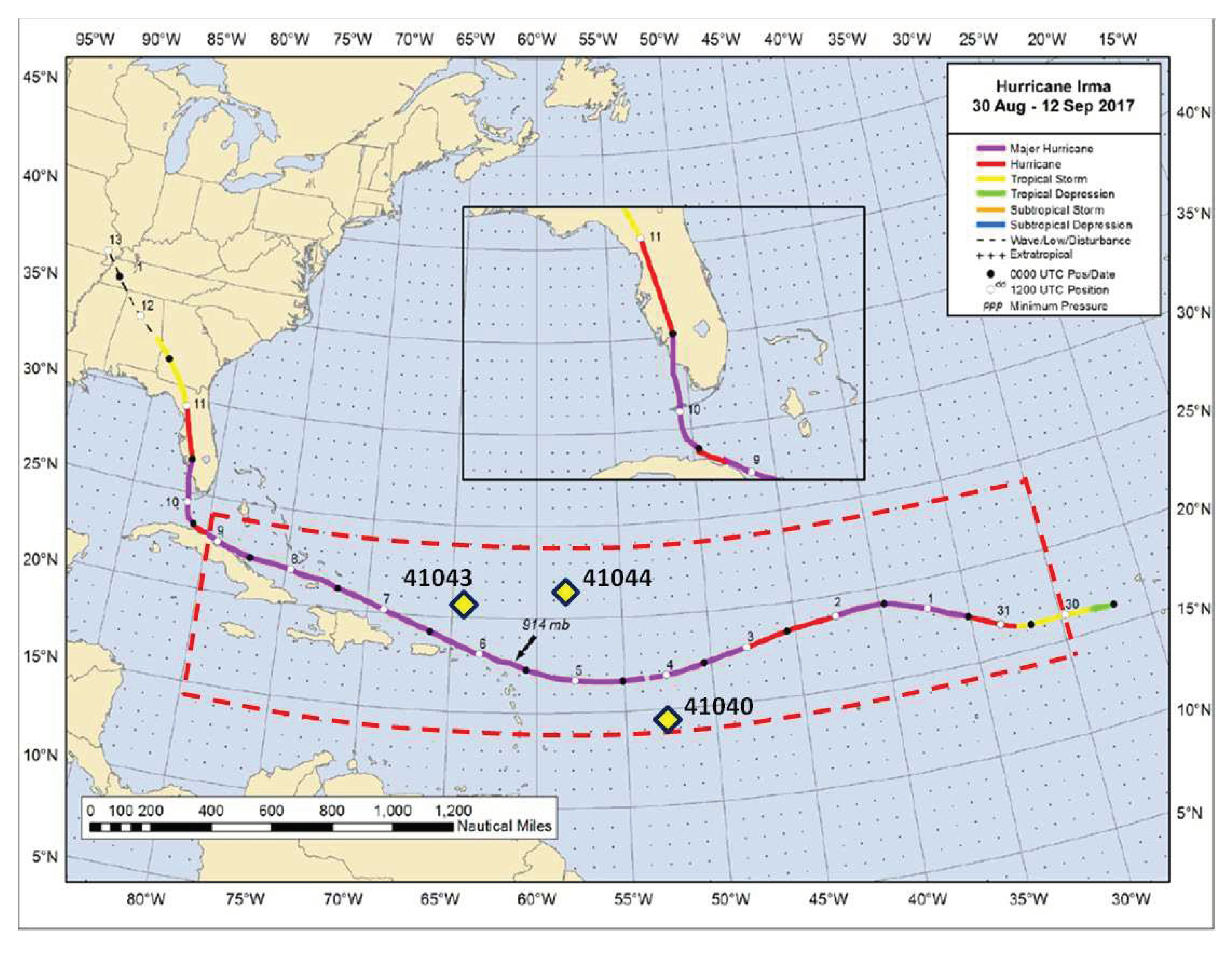
Figure 2.
The evolution of significant wave height distribution under hurricane Irma conditions simulated in WW3 with (a) ST4 wind input and (b) ST6 wind input at the fixed time. First line is the sea state on September 3, 2nd - September 5, 3d - September 6, 4th - September 7.
Figure 2.
The evolution of significant wave height distribution under hurricane Irma conditions simulated in WW3 with (a) ST4 wind input and (b) ST6 wind input at the fixed time. First line is the sea state on September 3, 2nd - September 5, 3d - September 6, 4th - September 7.
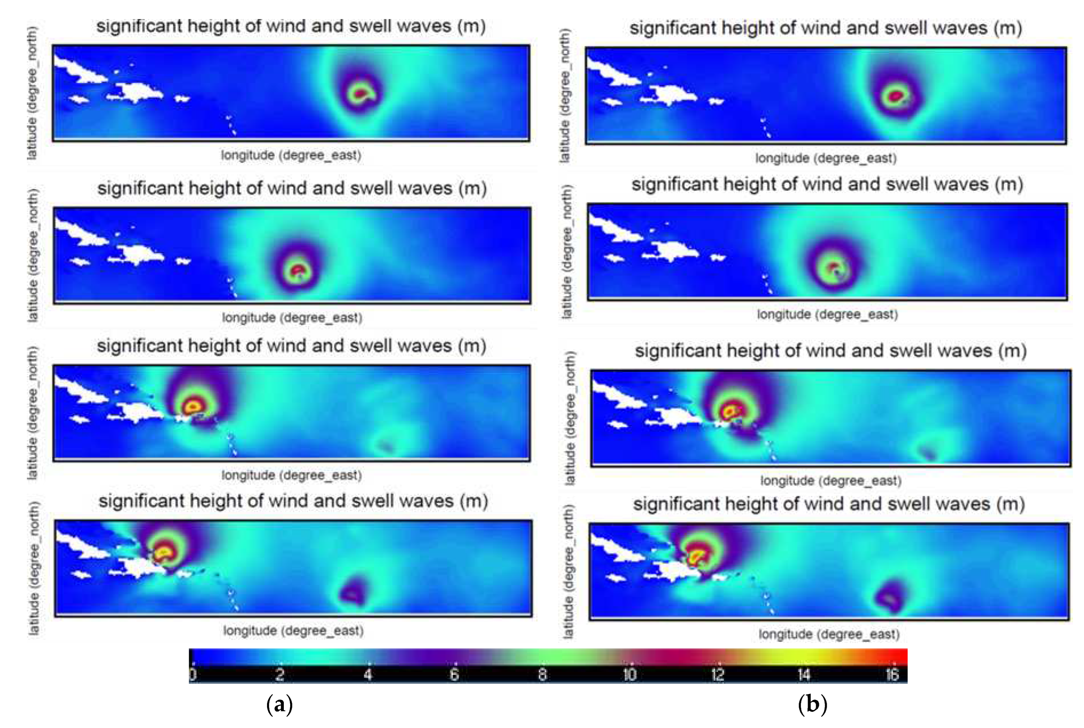
Figure 3.
a) The exact number of "parachutes" depending on the Reynolds number; b) the drag coefficient depending on the wind speed. Red line - estimates of the model from [9,11] for the wave age parameter Ω=3, symbols are presented for the available experimental data [26,27,28,29].
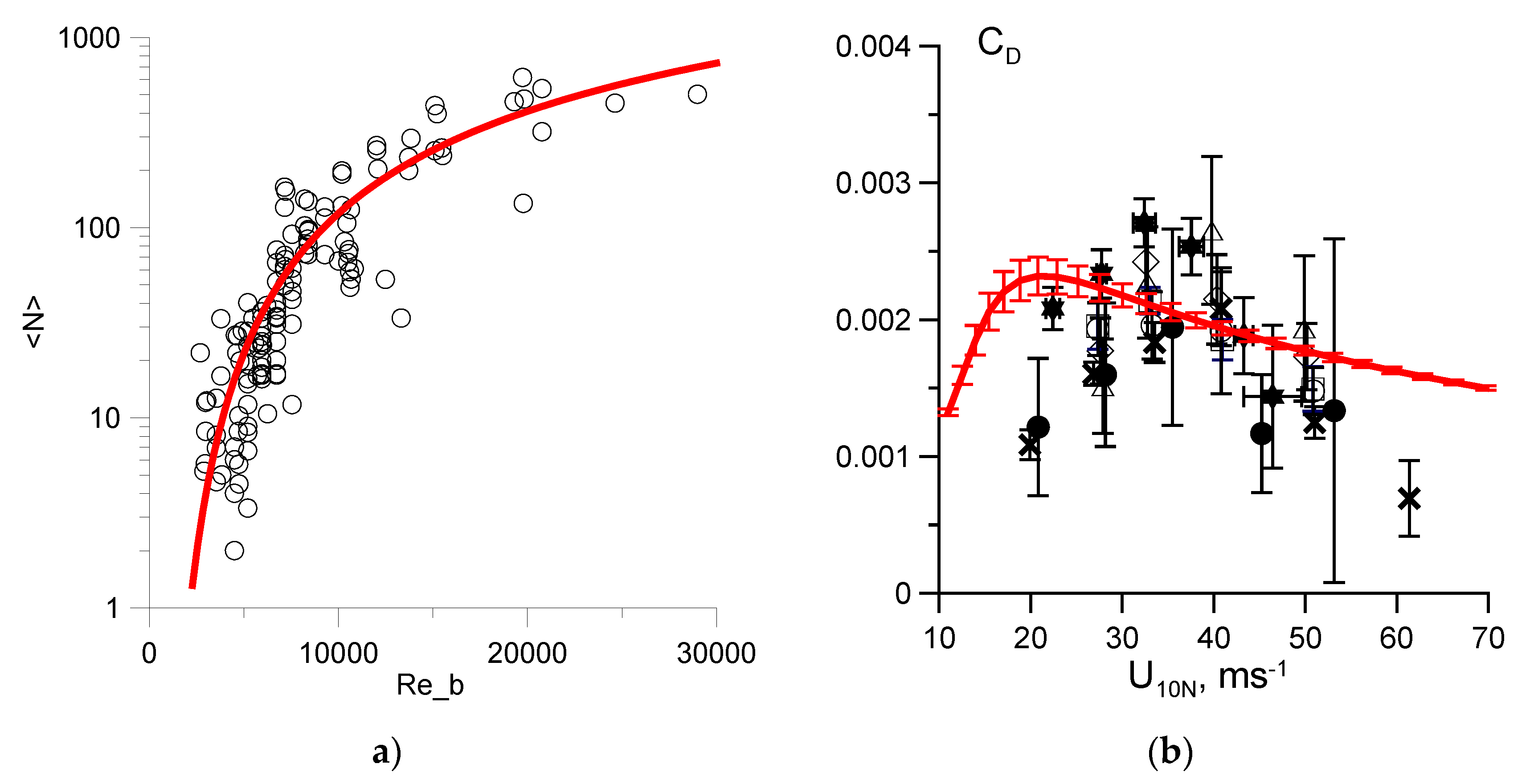
Figure 4.
(a) Wind speed distribution, black arrows indicate wind direction, large green arrow indicates hurricane direction, color scales are in m/s. (b) Spectrum peak frequency, the color scale is presented in Hz. (c) surface drag coefficient, the color scale is dimensionless. The horizontal axis is relative longitude, the vertical axis is relative latitude, both are in degrees.
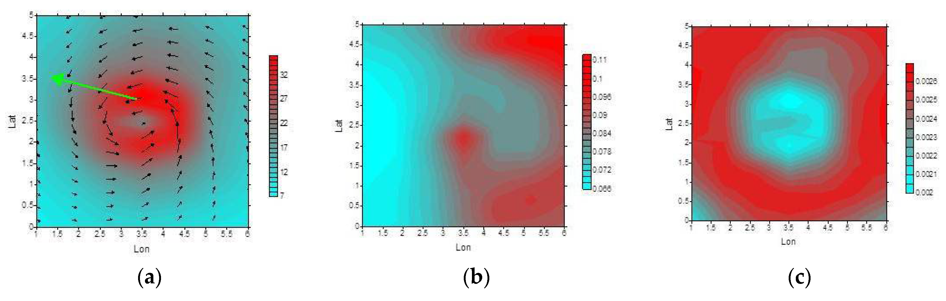
Figure 5.
Wave age time series in the simulation.
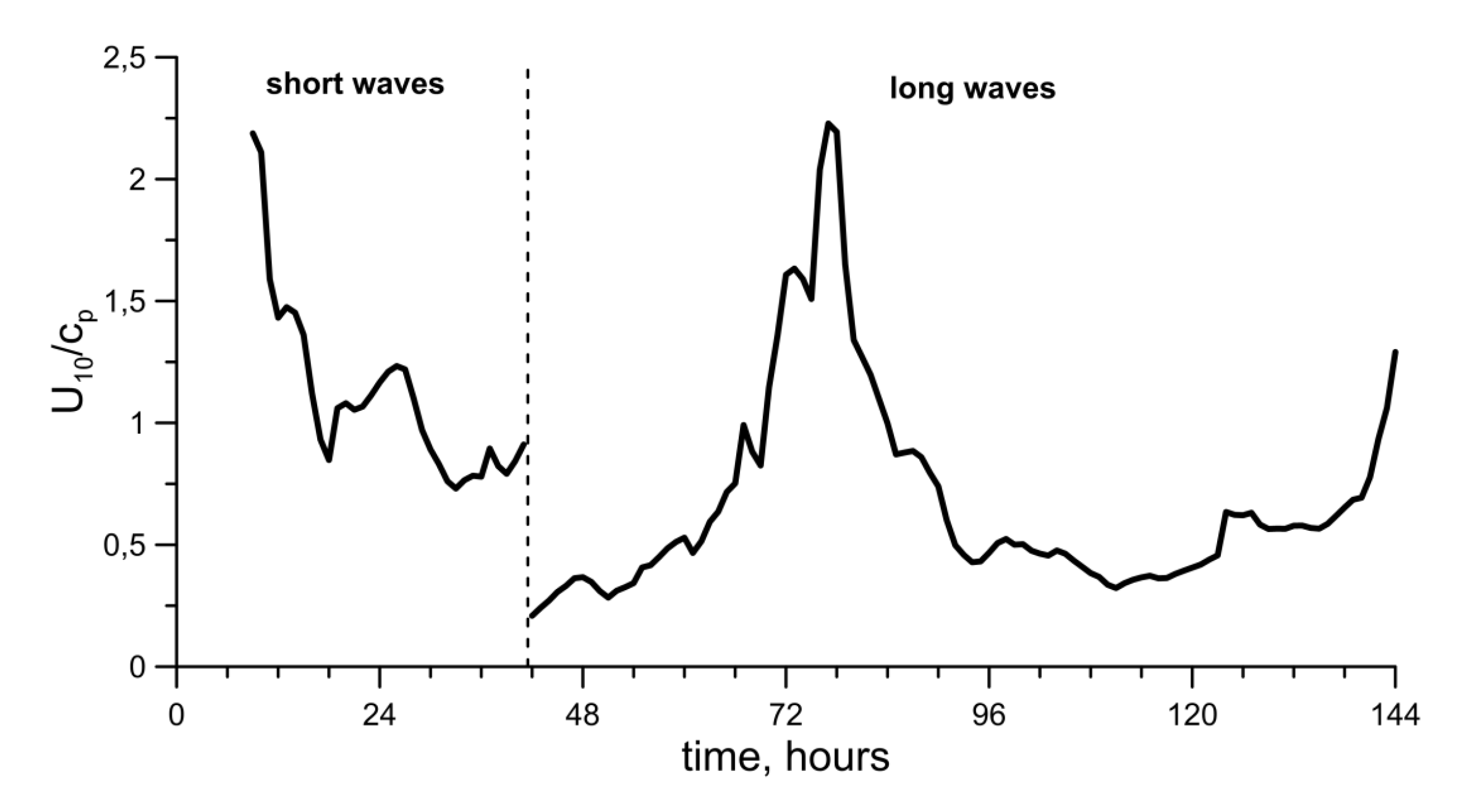
Figure 6.
Drag coefficient parameterization (a) CD spray ST1, dashed line is (8), blue line is resulting parameterization including spray and foam (22, 23) (b) CD spray ST6, dashed line is (18), red line is resulting parameterization including spray and foam (22, 23).
Figure 6.
Drag coefficient parameterization (a) CD spray ST1, dashed line is (8), blue line is resulting parameterization including spray and foam (22, 23) (b) CD spray ST6, dashed line is (18), red line is resulting parameterization including spray and foam (22, 23).
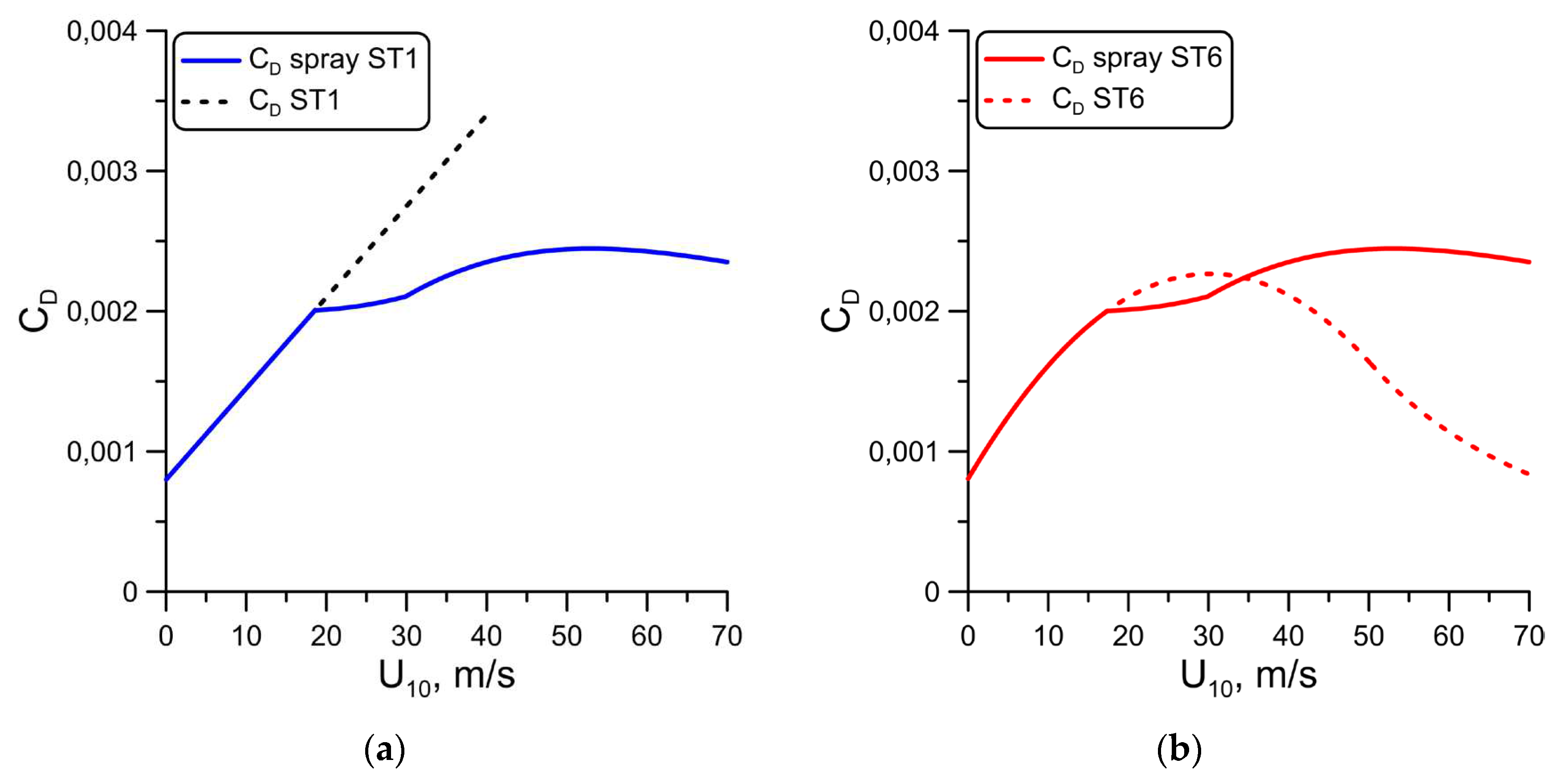
Figure 7.
The evolution of significant wave height distribution under hurricane Irma conditions simulated in WW3 with (a) ST1 CD spray (22, 23) wind input and (b) ST6 wind input CD spray (22, 23) at the fixed time. First line is the sea state on September 3, 2nd - September 5, 3d - September 6, 4th - September 7.
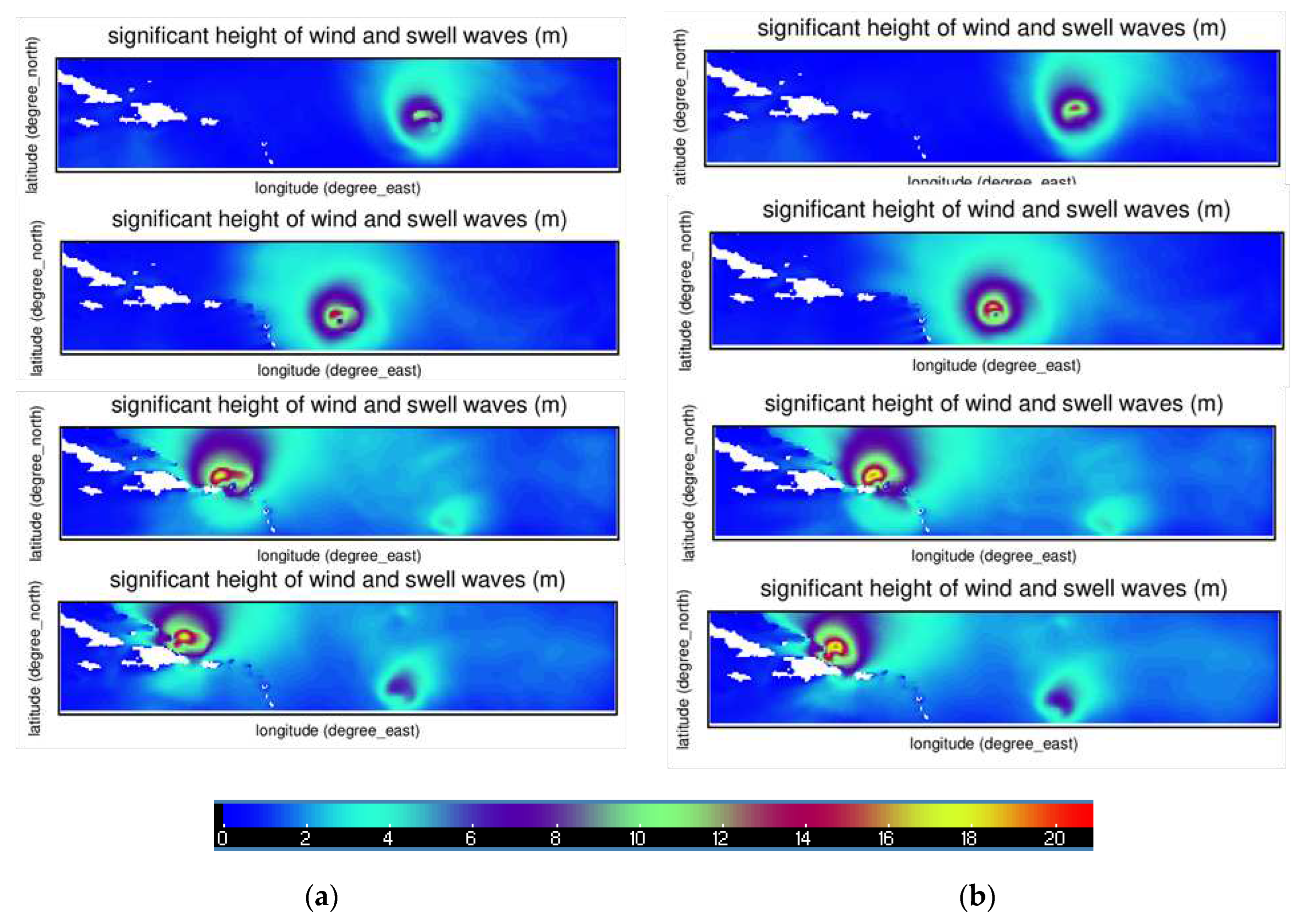
Figure 8.
Top: significant wave height simulated in WW3 with ST4 (green), ST6 (red dashed), ST6 with the CD spray (red), ST1 with the CD spray (blue) and buoy data (black). Down: 10 m wind speed for buoy data (black), CFSv2 reanalysis data (magenta). The data is shown for the period for the period from 02/09/2017 to 08/09/2017 for (a) – buoy 41040, (b) – buoy 41043, (c) – buoy 41044.

Disclaimer/Publisher’s Note: The statements, opinions and data contained in all publications are solely those of the individual author(s) and contributor(s) and not of MDPI and/or the editor(s). MDPI and/or the editor(s) disclaim responsibility for any injury to people or property resulting from any ideas, methods, instructions or products referred to in the content. |
© 2023 by the authors. Licensee MDPI, Basel, Switzerland. This article is an open access article distributed under the terms and conditions of the Creative Commons Attribution (CC BY) license (http://creativecommons.org/licenses/by/4.0/).
Copyright: This open access article is published under a Creative Commons CC BY 4.0 license, which permit the free download, distribution, and reuse, provided that the author and preprint are cited in any reuse.


