
Submitted:
28 April 2023
Posted:
28 April 2023
Read the latest preprint version here
Abstract
For order-of-addition experiments, the response is affected by the addition order of the experimental materials. Consequently, the main interest focuses on creating a predictive model and an optimal design for optimizing the response. Van Nostrand (1995) proposed the pairwise-order (PWO) model for detecting PWO effects. Under the PWO model, the full PWO design is optimal under various criteria but is often unaffordable because of the large run size. In this paper, we consider the D-, A- and M.S.-optimal fractional PWO designs. We first present some results on information matrices. Then, a flexible and efficient algorithm is given for generating these optimal PWO designs. Numerical simulation shows that the generated design has an appealing efficiency in comparison with the full PWO design, though with only a small fraction of runs. Several comparisons with existing designs illustrate that the generated designs achieve better efficiencies, and the best PWO designs and some selected 100% efficient PWO designs generated by the new algorithm are reported.
Keywords:
Pairwise-order model
; D-optimal
; A-optimal
; M.S.-optimal
; particle swarm optimization
; Fedorov exchange algorithm
1. Introduction
In some specific experiments, such as a chemical experiment with a number of reactants that are added into an apparatus sequentially rather than simultaneously, different orders of adding the components involved in the system yield different responses. Therefore, researchers are more interested in how the addition sequence of reactants affects the response. Experiments with this feature are referred to as order-of-addition (OofA) experiments and are widely applied to chemical-related areas and food industries, as well as biochemistry and measurement processes. The earliest research on OofA experiments can perhaps be traced back to the study of a lady tasting tea in Fisher (1937). Another study appeared in Fuleki and Francis (1968) that evaluated an experiment for extracting anthocyanins from cranberries. During the past decades, the approach of OofA experiments has been proposed in many practical studies; for example, see the references Jourdain et al. (2009), Karim, Mccormick, and Kappagoda (2000), Olsen et al. (1994) and so on.
For the objective of optimizing and predicting the response, a statistical model and an optimal design are created for the OofA experiment. The idea of pairwise-order (PWO) modeling and designing the OofA experiment has been presented in Van Nostrand (1995). Recently, Voelkel (2019) proposed a number of design criteria. Voelkel (2019) provided theoretical results on the full PWO design and construction of the optimal PWO design, which has the same correlation structure as the full PWO design, namely, the same information matrix. A recent review on OofA experiments and PWO models can be found in Lin and Peng (2019).
In fact, the PWO model is also a regression model. Then, a family of criteria can be applied to find optimal designs under the PWO model, such as D-, A- and -optimal designs. The optimality proof indicates that a full PWO design with distinct permutations of components is D-, A- and -optimal, but the run size is extremely large. Taking as an example, there are distinct permutations. Consequently, over three million runs of experiments should be implemented, which is impractical. Therefore, fractions of full PWO designs with a smaller number of runs are preferable.
Recently, four kinds of fractional PWO designs have been studied. Peng, Mukerjee, and Lin (2019) introduced a method for constructing optimal PWO designs. This method limits the run size to , which is also too many for experimenters to afford. For instance, if , the method needs at least 30240 runs to be implemented. Yang, Sun, and Xu (2021) and Zhao, Lin, and Liu (2022) provided construction methods based on an orthogonal array, the resulting designs are component orthogonal arrays (COAs) and OofA orthogonal arrays (OofA-OAs), in which the run size is also inflexible. Zhao, Lin and Liu (2021) provided a minimal-point design with runs. The run size is small, but the efficiency is relatively low. However, theoretical constructions of these fractional PWO designs are highly dependent on run size. Winker, Chen, and Lin (2020) applied the threshold accepting algorithm to construct the optimal designs (D-efficiency for application) based on the pairwise-order (PWO) model and the tapered PWO model, the designs obtained by threshold accepting algorithm for with respectively, are provided for practical uses. The present paper also provides a computer algorithm to construct the PWO design with a flexible run size, and D-, A-, and -optimal PWO designs can be constructed using the proposed algorithm. When compared with the full PWO designs, the constructed designs possess high efficiencies.
This paper is organized as follows. We first introduce the PWO model in Section 2. Section 3 gives a review of Fedorov’s exchange algorithm for constructing the D-optimal designs. Then, this algorithm is modified and extended for constructing A- and -optimal designs. Some theoretical results on the information matrix and algorithm are also provided in Section 3. In Section 4, based on the exchange algorithm and particle swarm optimization (PSO) algorithm, a novel hybrid algorithm is proposed to achieve D-, A- and -optimal PWO designs. Some numerical results are given in Section 5. Finally, concluding remarks are provided in Section 6.
2. Model specification
Now, we introduce the Van Nostrand PWO model. Suppose there are m components denoted as . Any treatment in the OofA experiment corresponds to a permutation of , denoted as , and the first-order PWO model can be expressed as
where each is a PWO indicator between j and k,
For an n-point PWO design, let Y be the n-dimensional response vector, Z be the design matrix with columns corresponding to PWO indicators , and , where denotes the transpose. Then, the first-order PWO model can be written as
or
where with is the model matrix, and represents the parameter of interest. Mee (2020) extended the PWO model to the high-order case. Here, we only consider a first-order PWO model. The proposed algorithms also apply to a higher-order PWO model.
Furthermore, we refer to as the information matrix of an n-point PWO design. Under the PWO model (3), the variance-covariance matrix of the least squares estimator of is proportional to . Hence, it is desirable to maximize the matrix under some criteria. The popular criteria include the D-criterion , the A-criterion , the -criterion (see the reference Atwood 1969). Note that is interpreted as for singular . Let be the full PWO design and the corresponding information matrix be . For clarity, we take as an example to illustrate the characteristics of the full PWO design under D-, A- and -criteria. The levels of PWO factors in the full PWO design with 3 components are as follows.

Table 1.
Full PWO design with 3 components
| Run | Order-of-Addition | |
|---|---|---|
| 1 | 1 2 3 | |
| 2 | 1 3 2 | |
| 3 | 2 1 3 | |
| 4 | 2 3 1 | |
| 5 | 3 1 2 | |
| 6 | 3 2 1 |
From this, we obtain
and and .
3. Exchange algorithms for constructing D-, A-, and -optimal designs
Theoretical constructions on optimal designs are always complicated; hence, computer algorithms are applied for constructing approximate and exact optimal designs in the literature. Exchange algorithm is one of the popular computer algorithms for constructing optimal designs for the cases with the design points being selected from a finite design space. Fedorov (1972) first proposed an exchange algorithm for generating D-optimal designs. This algorithm chooses n points to include in the design from a finite set of possible points called candidate points, and it starts with nonsingular n-point designs and then adds and deletes one observation in order to achieve increases in the determinant. After that some improved implementations are proposed based upon Fedorov’s exchange algorithm, such as the Kiefer round-off algorithm, the Mitchell algorithm, the Wan Schalkwyk algorithm, the combined Fedorov, the Wynn-Mitchell algorithm and so on; see the references Mitchell (1992), Nguyen and Miller (1992).
3.1. The single-point exchange procedure
Consider an n-point design under model (3), with a corresponding model matrix . If , then the D-, A- and -criteria maximize and respectively, which are equivalent to maximizing and respectively, where .
Inspired by Fedorov’s exchange algorithm, we develop a new exchange algorithm for generating D-, A- and -optimal designs simultaneously. This algorithm is realized by multiple iterations of the single-point exchange procedure which works as follows.
Single-point exchange procedure:
Let X be the model matrix of the original design and ,
- (1)
- Find a vector x among the vectors of the complementary design such that is maximum and add x to the current n-point design;
- (2)
- Find a vector among the vectors of the current -point design such that is minimum and remove .
When use the single-point exchange procedure for generating the D-, A- and -optimal designs, the objective functions are denoted as and with and defined as bellow:
where is the moment matrix of the current design and M is updated to when a candidate point from the complementary design is added to the current design. Here, the complementary design consists of all candidate points from the design space except for the n points of the current design.
Theorem 1.
The proof of this theorem uses some matrix theories, and we present it in the appendix. This result implies that exchange algorithm will return local D-, A- and -optimal designs over multiple iterations of the single-point exchange procedure.
3.2. The technique for avoiding the singularity of the matrix for the exchange algorithm
For generating optimal design using a computer search algorithm, the solution is often trapped into the local optimal design. Thus random exchange method is always used to avoid this drawback. For constructing D-, A- and -optimal designs using a computer search algorithm, a random selected initial design possibly corresponds to a singular moment matrix, especially for the case with a rather small number of n, and computation problem then arises. Taking the case with as an example. Among all options of n-point design, a large proportion of them correspond to a badly conditioned matrix M. As shown in Figure 1, all the reciprocal condition numbers are near 0, and the reciprocal condition number below is counted in the first bin of each histogram with a probability exceeding .
A random selected initial design will return a computationally singular matrix M with a large probability. For this reason, we address the issue of avoiding singularities of M and in the single-point exchange algorithm. Two types of techniques are provided regarding this issue. The first technique is to start with a nonsingular design instead of starting with a randomly selected design.
Remark 1.
If the initial design has nonsingular moment matrix, then by and , where , both and are nonsingular matrices during each iteration of the single-point exchange algorithm which is performed recursively.
This technique is practical since a nonsingular initial design with n points can be obtained by appending randomly selected distinct points to the minimal-point design provided in Zhao, Lin, and Liu (2021). However, in the hybrid algorithm, the design is updated via both the single-point exchange procedure and some random exchange procedure.
The second technique is inspired by the DETMAX algorithm in Mitchell (2000), a specified nonsingular matrix multiplied by a very small positive parameter is added to matrix M or . Taking M as an example, we do not consider directly, but instead attempt to calculate , where is the number of candidate points, and is the model matrix of the full design composed of all candidate points. Then, one technique that we can use to avoid the singularity of the matrix is as follows.
Remark 2.
To appreciate the degree of error involved in considering the alternative matrix, one can make the following calculations. Let
Then, extend in a Taylor series about to obtain the linear approximation:
For small , the error in considering instead of is nearly . In the proposed algorithm, the value of is set at 0.005, which is found to be quite satisfactory in simulations. This choice based on run size of the full PWO is sufficiently large such that , and the error will be less than .
Note that in this paper, we adopt the technique described in Remark 2 to avoid the singularity of the matrix.
3.3. The performance of the exchange algorithm
Now we discuss the performance of the exchange algorithm. The single-point exchange procedure is performed recursively, and the D-, A- and -efficiencies of the generated designs are calculated. For brevity, the cases with components are considered and the run sizes are fixed at . The following Figure 2 shows that the efficiencies are deeply increased in former iterations but then stabilized at slows on one value as the number of iterations increased. Therefore, the exchange algorithm yields locally optimal designs that approximate a global optimal design in a reasonable number of iterations.
To illustrate the performance of the exchange algorithm for constructing D-, A- and -optimal designs, 1000 designs are generated by the exchange algorithm with respective to each pair of the objective functions defined in equations (4)-(6). The initial designs are randomly selected. We list the minimum, average and maximum efficiencies of the generated designs in Table 2. Obviously, the generated designs are largely depended on the initial designs, most of them are locally optimal designs and some of them even have lower efficiencies than 80%, see the numbers in a bold font. Thus, in the next section, we proposed a more robust hybrid algorithm which combines the exchange algorithm and the particle swarm algorithm to produce approximate optimal designs with higher efficiency than the designs generated by exchange algorithm.
Table 2.
Efficiencies of 1000 designs generated by the exchange algorithm
| D-efficiency | A-efficiency | -efficiency | ||||||||
|---|---|---|---|---|---|---|---|---|---|---|
| m | Runs | Min | Ave | Max | Min | Ave | Max | Min | Ave | Max |
| 4 | 12 | 97.4% | 99.8% | 100% | 32.1% | 65.3% | 92.4% | 76.3% | 97.7% | 100% |
| 5 | 20 | 94.2% | 96.0% | 97.0% | 19.5% | 51.7% | 73.9% | 74.4% | 96.5% | 98.2% |
| 6 | 30 | 93.8% | 95.8% | 97.1% | 19.1% | 48.0% | 69.5% | 95.2% | 96.8% | 98.1% |
| 7 | 42 | 93.7% | 95.3% | 96.7% | 33.4% | 47.7% | 63.4% | 95.9% | 97.1% | 98.0% |
4. Constructions on D-, A- and -optimal PWO designs using a hybrid algorithm combining the exchange algorithm and PSO algorithm
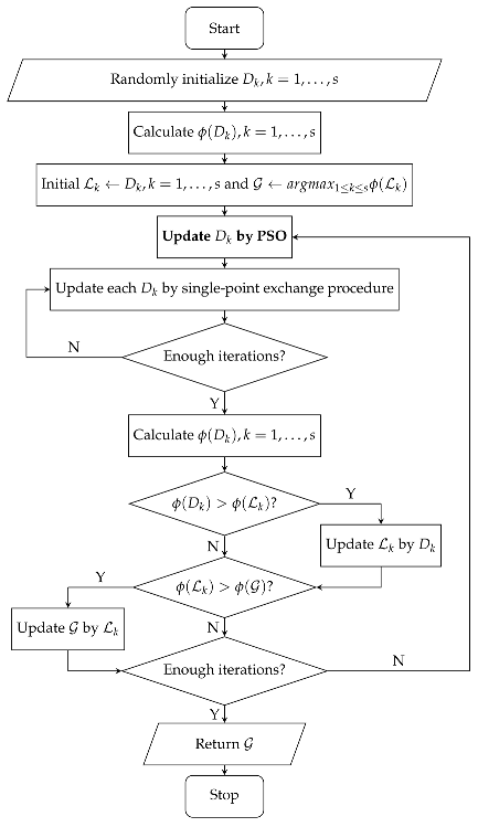
Before introducing the new algorithm, we add some details of the PSO algorithm. PSO is a population-based stochastic algorithm for optimization. Each population member is described as a particle that moves around a search space testing new criterion values. All particles survive from the beginning of a trial until the end, and their interactions result in iterative improvement of the quality of the problem solutions over time. The most common type of implementation defines the particles’ behavior as adjusting toward each of its personal best position(local-best) and global-best position so that its trajectory shifts to new regions of the search space and the particles gradually cluster around the optima. For applications to find optimal experimental designs, a particularly challenging task is to redefine the particle designs’ movement toward its personal local-best design and global-best design. A review of some recent applications of PSO and its variants to tackle various types of efficient experimental design is Chen, Chen, and Wang (2022). Since finding optimal PWO designs for OofA experiment is to solve a discrete optimization problem, we utilize a update procedure for the particle designs that is similar to the modified PSO algorithms in Chen et al. (2014) and Phoa et al. (2016). Each particle design relates to its personal local-best design which is derived by exchange procedures starting from itself. During each iteration, the current particle design is adjusted toward its personal local-best design as well as the global-best design by exchanging points with each other.
Now, we introduce a new hybrid algorithm called Ex-PSO algorithm, which combining the single-point exchange algorithm and PSO algorithm for generating D-, A-, and -optimal designs. The single-point exchange algorithm is used for generating the local-best design with respect to each particle design. The PSO algorithm ensure the particle designs gradually cluster around the optimal PWO design. To avoid singularity, the technique proposed in Remark 2 is used; hence, a parameter with a small value is involved in this algorithm.
Since the Ex-PSO algorithm involves a set of parameters denoted as , we also refer to it as Ex-PSO for generating optimal PWO design with m components and n runs. For clarity, we create a programming chart to illustrate the steps of Ex-PSO. Further, we explain the optimization process and the uses of these parameters as follows. Denote s and as the local-best designs and the global-best design respectively. These designs are updated during each iteration of the Ex-PSO algorithm. Each local-best design is derived from the current particle design via a fixed number of iterations of the single-point exchange procedure, denoted as . In addition, the global-best design is the optimal local-best design that maximizes . And the number of iterations of the PSO algorithm is denoted as . Meanwhile, two parameters are used to control the PSO behavior of the Ex-PSO algorithm: and , which account for the velocities at which each current design drifts toward the corresponding local-best and global-best design. More specifically, during each iteration of the PSO algorithm, we randomly exchange points from the difference set with points from and then randomly exchange points from the difference set with points from . This procedure corresponds to the “Update by PSO" box in the programming chart.
Finally, we note that the Ex-PSO algorithm is implemented in MATLAB running on Intel(R) Core(TM) i7-8550U GHz with 8 GB Memory. Take the case of for example, it takes 30.42 seconds for running Ex-PSO.
5. Numerical simulations
In this section, we illustrate the performances of the obtained designs constructed by the Ex-PSO algorithm. For brevity, the generated designs are denoted as Ex-PSO-D, Ex-PSO-A and Ex-PSO-M.S. designs that respectively correspond to the objective functions (4)-(6) which are considered in the exchange algorithm. Numerical simulations show that these designs are powerful for fitting PWO models in terms of the D-, A- and -efficiencies. The efficiencies are derived from comparison with the full PWO design, since the information matrix of the full PWO design has been proven to be universally optimal. Therefore, we have the D-, A- and -efficiencies that calculate , and respectively, where and are the information matrices of the obtained design and full PWO design respectively, and p is the number of the columns of the model matrix X.
Ex-PSOAlgorithm: Ex-PSO
Clearly, the number of PSO particles (s), the maximum iteration counts of single-point exchange algorithm and PSO algorithm () and the numbers of pairs of exchanging points with which each particle design drifts toward the local-best and global-best design , control the optimization process of Ex-PSO algorithm. It seems reasonable that these parameters should be larger for larger problems. In our test of searching for optimal PWO designs with components, we recommend that these parameters to set at , , , . Furthermore, we recommend to set the maximum iteration counts of exchange algorithm and PSO at and respectively, which achieves high computational efficiency. Further, to demonstrate the performance of such a set of parameters, we randomly run the algorithm Ex-PSO for one hundred times for generating the Ex-PSO-A designs, because the exchange algorithm seems inefficient under A-optimal criterion, as shown in Table 2. Therefore, one hundred Ex-PSO-A designs with components and runs are generated, and Figure 3 highlights that all Ex-PSO-A designs reach at least of the efficiency of the full PWO design. For the cases with large m, the settings on maximum iterations, and may not be enough, but the Ex-PSO algorithm still returns approximate optimal PWO designs; see Tables 4-6 in the following part.
To illustrate the advantages of the obtained designs for fitting PWO model, we compare the Ex-PSO-D designs for 4 components and 12 runs with the optimal PWO design in Peng, Mukerjee, and Lin (2019).
Example 1.
The following is aEx-PSO-Ddesign with 4 components and 12 runs generated by Ex-PSO.
The information matrix of this design under the first-order PWO model is
If rows are rearranged, this design is the same as the optimal PWO design with runs constructed by Peng, Mukerjee, and Lin (2019). This design also features projective properties (Voelkel and Gallagher 2019). All 4 subsets of three components correspond to two-times-replicated three-component designs.
Table 3.
An Ex-PSO-D design with 4 components and 12 runs
| Run | Order-of-Addition | |
|---|---|---|
| 1 | 1 4 2 3 | |
| 2 | 1 2 4 3 | |
| 3 | 1 3 2 4 | |
| 4 | 2 1 3 4 | |
| 5 | 2 4 3 1 | |
| 6 | 2 3 4 1 | |
| 7 | 3 1 4 2 | |
| 8 | 3 2 1 4 | |
| 9 | 3 4 1 2 | |
| 10 | 4 1 3 2 | |
| 11 | 4 2 1 3 | |
| 12 | 4 3 2 1 |
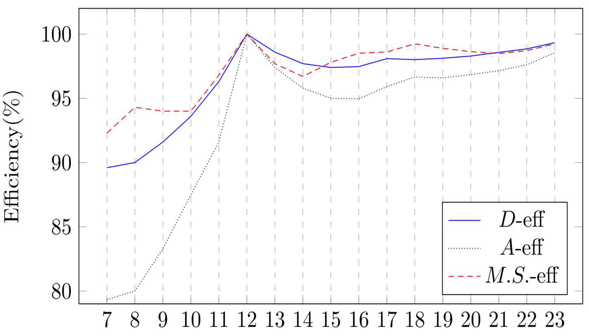
Furthermore, for the OofA experiment with 4 components, we generated optimal PWO designs with 7 to 23 runs using the Ex-PSO algorithm. Figure 4 shows the efficiencies of these designs. Clearly, all the obtained designs with reach at least efficiency of the full PWO design, though with less than one fifth of the runs. Especially for the cases with , the design attains the same efficiency as the full PWO design.
Furthermore, we compare four types of fractional PWO designs, which are COA, and the corresponding designs obtained by the threshold accepting algorithm (Winker, Chen, and Lin 2020), the Federov’s exchange algorithm (which iteratively optimizes a delta function of the and x where is in the design and x is not, see reference to section 3.3 in Fedorov 1972) and the Ex-PSO algorithm, denoted as , , and respectively. is the best result obtained over repeated runs of threshold accepting algorithm with up to 10000000 iterations, is generated by the optFederov function (implemented in the R library AlgDesign) with , and is the best result obtained over five repeated runs of the Ex-PSO algorithm with and . The optimal PWO design constructed in Peng, Mukerjee, and Lin (2019) which serves as a benchmark for evaluating fractional PWO designs is also listed here and denoted as . In addition, the new hybrid algorithm needs exhaustive search over the design space during the single-point exchange procedure, and it can be computational expensive if m is large. Hence, we only report designs with where . Nevertheless, given the tremendous growth in computational resources available, it is feasible to conduct the Ex-PSO algorithm for constructing designs with .
Tables 4-6 exhibit the values of , , , and D-, A- and -efficiency (in parentheses) for the corresponding designs. Note that the larger the value of is, the better, while smaller values of and are better. For any number of components, is not unique and the corresponding or is by no means a fixed value. Hence, is not listed in Tables 5 and 6. From the tables, we can find that reach a higher efficiency than the other types of designs under the PWO model in most cases. Further, we report the best PWO designs with and under the D-, A- and -optimal criteria in the supplementary material.
Table 4.
Comparison of and D-efficiency of PWO designs
| m | n | |||||
|---|---|---|---|---|---|---|
| 4 | 7 | - | - | 0.6966(89.6%) | 0.6966(89.6%) | 0.6966(89.6%) |
| 12 | 0.7773(100%) | 0.7064(90.9%) | 0.7773(100%) | 0.7773(100%) | 0.7773(100%) | |
| 5 | 11 | - | - | 0.6379(90.3%) | 0.6211(87.9%) | 0.6379(90.3%) |
| 20 | - | 0.6354(89.9%) | 0.6855(97.0%) | 0.6840(96.8%) | 0.6855(97.0%) | |
| 60 | 0.7067(100%) | - | 0.7067(100%) | 0.7061(99.9%) | 0.7067(100%) | |
| 6 | 16 | - | - | 0.5778(88.1%) | 0.5612(85.6%) | 0.6002(91.5%) |
| 30 | - | 0.5710(87.1%) | 0.6344(96.7%) | 0.6372(97.2%) | 0.6381(97.3%) | |
| 120 | 0.6558(100%) | - | 0.6552(99.9%) | 0.6555(99.95%) | 0.6558(100%) | |
| 7 | 22 | - | - | 0.5016(81.2%) | 0.5325(86.2%) | 0.5409(87.6%) |
| 42 | - | 0.5800(93.9%) | 0.5958(96.4%) | 0.5996(97.0%) | 0.5998(97.1%) | |
| 840 | 0.6178(100%) | - | 0.6178(100%) | 0.6177(99.99%) | 0.6178(100%) |
Table 5.
Comparison of and A-efficiency of PWO designs
| m | n | |||||
|---|---|---|---|---|---|---|
| 4 | 7 | - | - | 17.5000(67.4%) | - | 14.8750(79.3%) |
| 12 | 11.8000(100%) | 14.5000(81.4%) | 11.8000(100%) | 11.8000(100%) | 11.8000(100%) | |
| 5 | 11 | - | - | 28.2898(74.2%) | - | 26.4773(79.3%) |
| 20 | - | 26.0000(80.8%) | 22.4550(93.5%) | 22.3910(93.8%) | 22.3311(94.0%) | |
| 60 | 21.0000(100%) | - | 21.0337(99.8%) | 21.0000(100%) | 21.0000(100%) | |
| 6 | 16 | - | - | 46.0558(72.0%) | - | 40.8428(81.2%) |
| 30 | - | 45.3736(73.0%) | 35.3203(93.8%) | 35.0989(94.4%) | 35.0144(94.7%) | |
| 120 | 33.1429(100%) | - | 33.2443(99.7%) | 33.2023(99.8%) | 33.1721(99.9%) | |
| 7 | 22 | - | - | 76.4729(63.1%) | - | 72.4088(66.6%) |
| 42 | - | 57.1177(84.5%) | 51.6845(93.4%) | 51.0578(94.5%) | 51.5024(93.7%) | |
| 840 | 48.2500(100%) | - | 48.2583(99.98%) | 48.2738(99.95%) | 48.2555(99.99%) | |
| Note: with is omitted because it reports an error of “singular design" | ||||||
| when running the optFederov function from the AlgDesign package in R. | ||||||
Table 6.
Comparison of and -efficiency of PWO designs
| m | n | ||||
|---|---|---|---|---|---|
| 4 | 7 | - | - | 10.4694(92.3%) | 10.4694(92.3%) |
| 12 | 9.6667(100%) | 10.3333(93.6%) | 9.6667(100%) | 9.6667(100%) | |
| 5 | 11 | - | - | 18.5207(95.4%) | 18.5207(95.4%) |
| 20 | - | 19.0000(93.0%) | 18.0400(97.9%) | 18.0000(98.2%) | |
| 60 | 17.6667(100%) | - | 17.6667 (100%) | 17.6667(100%) | |
| 6 | 16 | - | - | 31.0000(94.6%) | 30.9688(94.7%) |
| 30 | - | 31.3333(93.6%) | 29.8756(98.2%) | 29.8311(98.3%) | |
| 120 | 29.3333(100%) | - | 29.3556(99.92%) | 29.3733(99.89%) | |
| 7 | 22 | - | - | 47.5702(95.3%) | 47.7686(94.9%) |
| 42 | - | 45.8095(99.0%) | 45.9048 (98.8%) | 46.1905(98.1%) | |
| 840 | 45.3333(100%) | - | 45.3349(99.99%) | 45.3368(99.99%) |
We conclude this section with some numerical results on constructions of fractional PWO designs which have the same correlation structure as the full PWO design. Since these designs are 100% efficient under diverse design criteria including the D-, A-, -optimal criteria, we call them fully efficient PWO designs. Using the Ex-PSO algorithm, we find the following results.
Remark 3.
Removing components from a fully efficient PWO design with m components will result in a fully efficient PWO design with components.
Remark 4.
The fully efficient PWO designs exist for the cases (i) , ; (ii) , ; and (iii) , .
For saving space, some selected fully efficient PWO designs with minimized runs for are exhibited in Table 7, other fully efficient PWO designs and the MATLAB codes for the Ex-PSO algorithm are available upon request.
Table 7.
Selected fully efficient PWO designs for
| runs 1-12 | runs 13-24 | runs 1-12 | runs 13-24 | ||
| 1 2 4 3 | 1 2 3 5 4 | 1 2 5 4 6 3 | 4 2 1 3 6 5 | 1 2 3 7 4 6 5 | 4 5 2 6 7 1 3 |
| 1 3 4 2 | 1 4 3 5 2 | 1 2 5 4 6 3 | 4 2 5 3 6 1 | 1 5 6 3 2 7 4 | 4 6 3 7 1 2 5 |
| 1 3 2 4 | 1 5 3 2 4 | 1 3 4 2 5 6 | 4 6 3 2 5 1 | 1 6 5 7 4 2 3 | 4 7 1 3 6 5 2 |
| 2 1 4 3 | 2 4 3 1 5 | 1 3 6 2 5 4 | 5 1 2 4 3 6 | 1 7 4 3 2 5 6 | 5 2 4 3 6 1 7 |
| 2 3 1 4 | 2 5 1 4 3 | 1 4 6 5 2 3 | 5 4 3 2 1 6 | 2 5 4 1 7 6 3 | 6 1 2 4 5 7 3 |
| 2 3 4 1 | 3 1 4 2 5 | 2 3 4 5 1 6 | 5 2 1 6 3 4 | 2 7 6 3 1 5 4 | 6 4 2 1 3 7 5 |
| 3 1 4 2 | 3 2 4 5 1 | 2 6 1 5 3 4 | 5 3 6 2 1 4 | 3 2 1 6 4 7 5 | 6 5 1 3 4 7 2 |
| 3 2 4 1 | 3 5 4 2 1 | 2 6 4 3 1 5 | 5 6 4 1 2 3 | 3 2 6 5 7 4 1 | 6 7 2 3 4 5 1 |
| 4 1 2 3 | 4 2 1 5 3 | 3 1 2 6 4 5 | 6 2 1 4 3 5 | 3 4 1 5 7 2 6 | 7 4 6 5 3 2 1 |
| 4 2 1 3 | 4 5 1 2 3 | 3 1 5 6 4 2 | 6 2 5 3 4 1 | 3 5 1 4 6 2 7 | 7 2 1 5 3 4 6 |
| 4 3 1 2 | 5 2 3 1 4 | 3 5 2 4 6 1 | 6 3 5 1 4 2 | 3 5 7 6 2 1 4 | 7 5 1 2 6 4 3 |
| 4 3 2 1 | 5 4 3 1 2 | 4 1 5 6 3 2 | 6 4 5 1 3 2 | 4 2 5 3 7 1 6 | 7 5 3 6 4 1 2 |
6. Concluding Remarks
For the OofA experiments, the study of the optimal fraction of the PWO design has received considerable attention in the literature. The fractional PWO design with the same correlation structure as the full PWO design is optimal under diverse design criteria but exists only for some fixed run sizes, such as runs. Theoretical constructions on optimal PWO designs are also heavily constrained by the run size. In this paper, we present a flexible and effective searching algorithm, the Ex-PSO algorithm. Even though the candidate fractional PWO designs are extremely massive, this algorithm generates high efficient designs with only one hundred iterations. Moreover, it’s an interesting but difficult problem to obtain more general theoretical results which cover Remark 4 as special cases. While Remark 3 gives a fresh insight into constructions of the fully efficient PWO design with m components basing on the fully efficient PWO design with components. To that effect, more theoretical results on the fully efficient PWO designs for general m will be studied in our future work.
It is worth noting that the Ex-PSO designs are possibly to an optimal PWO designs given the tremendous growth in computational resources available, thus it provides instructions for exploring theoretical results on optimal PWO designs. In addition, the Ex-PSO algorithm applies not only to PWO design but also to any type of design with finite candidate points. Therefore, this algorithm has many potential applications, such as constructing optimal designs for an alternative model of the OofA experiment or other kinds of experiments, and there are still many issues for further study.
Acknowledgments
The authors thank the editor and two referees for their valuable comments and suggestions. This work was supported by the National Natural Science Foundation of China (grant nos. 11971098, 11971097, 12101258 and 12131001), National Key Research and Development Program of China (No. 2020YFA0714102) and Education Department Science and Technology Project of Jilin Province under Grant JJKH20220152KJ.
Appendix A. The proof of Theorem 1
To prove Theorem 1, the following two lemmas are useful.
Lemma A.1.For a nonsingular matrix M,
- (1)
- is nonsingular, and , where ;
- (2)
- if is nonsingular, then and , where .
The proof of this lemma is straightforward according to matrix theory and is thus omitted.
Lemma A.2.Let M be a nonsingular matrix and ; we have and .
Proof: According to Lemma A.1, we have
and
Proof of Theorem 1
Since Fedorov’s exchange algorithm has proved this result for the case with , and defined as Equation (4), hence we only prove this result for the other two cases.
First, we prove that the design generated by single-point exchange procedure leads to no increase in .
Let X be the model matrix of the current design and denote , which is updated as after exchanging x for according to the single exchange procedure. The following delta function evaluates the multiple changes from to :
Based on step (2) of this procedure, we know that . In the combination of Lemma A.2, we obtain
Thus, is obtained, which means does not increase in the single-point exchange procedure.
Second, we prove that the design generated in single-point procedure leads to no increase in .
To calculate the multiple exchange on the during each iteration of the single-point exchange procedure, we define a delta function as follows:
By step (2) of this procedure, we have and
Theorem 1 is proved.
Appendix B. Best PWO designs under the D-optimal criterion
Table B.1.
D-Optimal PWO designs for
| 7 runs | 12 runs | ||||||||||
|---|---|---|---|---|---|---|---|---|---|---|---|
| runs 1-7 | runs 8-12 | ||||||||||
| 1 | 2 | 3 | 4 | 1 | 2 | 4 | 3 | 3 | 2 | 1 | 4 |
| 1 | 3 | 4 | 2 | 1 | 2 | 3 | 4 | 3 | 2 | 4 | 1 |
| 2 | 1 | 4 | 3 | 1 | 3 | 4 | 2 | 4 | 1 | 3 | 2 |
| 3 | 1 | 2 | 4 | 2 | 1 | 4 | 3 | 4 | 2 | 1 | 3 |
| 3 | 2 | 4 | 1 | 2 | 3 | 4 | 1 | 4 | 2 | 3 | 1 |
| 4 | 1 | 3 | 2 | 3 | 1 | 4 | 2 | 4 | 3 | 1 | 2 |
| 4 | 2 | 3 | 1 | ||||||||
Table B.2.
D-Optimal PWO designs for
| 11 runs | 20 runs | |||||||||||||
|---|---|---|---|---|---|---|---|---|---|---|---|---|---|---|
| runs 1-10 | runs 11-20 | |||||||||||||
| 1 | 5 | 3 | 4 | 2 | 1 | 5 | 2 | 3 | 4 | 3 | 5 | 4 | 1 | 2 |
| 2 | 5 | 3 | 4 | 1 | 1 | 2 | 5 | 4 | 3 | 3 | 4 | 2 | 1 | 5 |
| 2 | 3 | 1 | 4 | 5 | 1 | 3 | 4 | 2 | 5 | 4 | 1 | 5 | 3 | 2 |
| 2 | 4 | 1 | 3 | 5 | 1 | 4 | 2 | 3 | 5 | 4 | 3 | 1 | 5 | 2 |
| 3 | 2 | 5 | 1 | 4 | 2 | 1 | 4 | 3 | 5 | 4 | 3 | 5 | 1 | 2 |
| 3 | 4 | 5 | 1 | 2 | 2 | 5 | 4 | 1 | 3 | 4 | 5 | 3 | 2 | 1 |
| 4 | 2 | 5 | 1 | 3 | 2 | 3 | 4 | 5 | 1 | 5 | 1 | 3 | 2 | 4 |
| 4 | 3 | 1 | 2 | 5 | 2 | 4 | 5 | 3 | 1 | 5 | 2 | 3 | 1 | 4 |
| 4 | 5 | 3 | 2 | 1 | 3 | 2 | 1 | 5 | 4 | 5 | 3 | 1 | 4 | 2 |
| 5 | 1 | 2 | 4 | 3 | 3 | 5 | 2 | 1 | 4 | 5 | 4 | 2 | 1 | 3 |
| 5 | 4 | 2 | 3 | 1 | ||||||||||
Table B.3.
D-Optimal PWO designs for
| 16 runs | 30 runs | ||||||||||||||||
|---|---|---|---|---|---|---|---|---|---|---|---|---|---|---|---|---|---|
| runs 1-15 | runs 16-30 | ||||||||||||||||
| 1 | 6 | 5 | 2 | 4 | 3 | 1 | 6 | 2 | 5 | 3 | 4 | 4 | 5 | 1 | 6 | 2 | 3 |
| 1 | 2 | 4 | 5 | 3 | 6 | 1 | 2 | 6 | 3 | 5 | 4 | 4 | 5 | 2 | 6 | 1 | 3 |
| 1 | 5 | 3 | 6 | 4 | 2 | 1 | 3 | 4 | 2 | 5 | 6 | 4 | 5 | 3 | 1 | 2 | 6 |
| 2 | 1 | 3 | 5 | 4 | 6 | 1 | 4 | 6 | 3 | 5 | 2 | 5 | 2 | 1 | 3 | 6 | 4 |
| 2 | 3 | 6 | 5 | 4 | 1 | 2 | 1 | 5 | 4 | 6 | 3 | 5 | 2 | 3 | 1 | 4 | 6 |
| 3 | 1 | 4 | 2 | 6 | 5 | 2 | 6 | 4 | 1 | 5 | 3 | 5 | 4 | 1 | 3 | 6 | 2 |
| 3 | 2 | 5 | 1 | 6 | 4 | 2 | 3 | 5 | 4 | 6 | 1 | 5 | 4 | 3 | 6 | 1 | 2 |
| 3 | 4 | 5 | 1 | 6 | 2 | 3 | 1 | 5 | 2 | 6 | 4 | 5 | 6 | 3 | 1 | 2 | 4 |
| 4 | 1 | 3 | 5 | 2 | 6 | 3 | 1 | 6 | 4 | 2 | 5 | 5 | 6 | 3 | 4 | 2 | 1 |
| 4 | 2 | 5 | 1 | 6 | 3 | 3 | 2 | 6 | 5 | 1 | 4 | 6 | 1 | 5 | 4 | 2 | 3 |
| 4 | 3 | 6 | 5 | 2 | 1 | 3 | 2 | 4 | 1 | 6 | 5 | 6 | 1 | 2 | 3 | 4 | 5 |
| 5 | 2 | 6 | 3 | 1 | 4 | 3 | 4 | 6 | 1 | 5 | 2 | 6 | 2 | 1 | 4 | 5 | 3 |
| 5 | 4 | 6 | 3 | 1 | 2 | 3 | 5 | 6 | 2 | 1 | 4 | 6 | 2 | 4 | 3 | 5 | 1 |
| 6 | 1 | 4 | 2 | 3 | 5 | 4 | 2 | 1 | 3 | 5 | 6 | 6 | 3 | 5 | 4 | 2 | 1 |
| 6 | 3 | 2 | 4 | 1 | 5 | 4 | 2 | 6 | 5 | 3 | 1 | 6 | 5 | 1 | 3 | 2 | 4 |
| 6 | 5 | 1 | 3 | 2 | 4 | ||||||||||||
Table B.4.
D-Optimal PWO designs for
| 22 runs | 42 runs | |||||||||||||||||||
|---|---|---|---|---|---|---|---|---|---|---|---|---|---|---|---|---|---|---|---|---|
| runs 1-21 | runs 22-42 | |||||||||||||||||||
| 1 | 7 | 5 | 2 | 6 | 4 | 3 | 1 | 7 | 6 | 5 | 2 | 3 | 4 | 4 | 3 | 7 | 5 | 6 | 2 | 1 |
| 1 | 4 | 3 | 6 | 5 | 7 | 2 | 1 | 4 | 7 | 2 | 3 | 6 | 5 | 4 | 7 | 2 | 1 | 5 | 6 | 3 |
| 2 | 5 | 6 | 1 | 3 | 4 | 7 | 1 | 4 | 3 | 2 | 7 | 6 | 5 | 4 | 6 | 2 | 1 | 7 | 5 | 3 |
| 2 | 6 | 3 | 4 | 7 | 1 | 5 | 1 | 5 | 6 | 4 | 2 | 7 | 3 | 4 | 6 | 5 | 3 | 7 | 1 | 2 |
| 3 | 1 | 2 | 5 | 6 | 7 | 4 | 1 | 6 | 2 | 4 | 5 | 3 | 7 | 5 | 1 | 6 | 4 | 7 | 3 | 2 |
| 3 | 2 | 7 | 4 | 6 | 5 | 1 | 2 | 1 | 4 | 3 | 6 | 7 | 5 | 5 | 2 | 1 | 7 | 4 | 6 | 3 |
| 3 | 7 | 5 | 6 | 1 | 4 | 2 | 2 | 3 | 7 | 1 | 6 | 4 | 5 | 5 | 2 | 3 | 6 | 4 | 1 | 7 |
| 3 | 5 | 4 | 1 | 7 | 6 | 2 | 2 | 3 | 5 | 4 | 7 | 6 | 1 | 5 | 3 | 1 | 4 | 6 | 7 | 2 |
| 4 | 2 | 1 | 7 | 5 | 3 | 6 | 2 | 5 | 7 | 1 | 3 | 4 | 6 | 5 | 7 | 2 | 6 | 1 | 4 | 3 |
| 4 | 5 | 6 | 1 | 2 | 7 | 3 | 2 | 5 | 4 | 7 | 3 | 6 | 1 | 6 | 1 | 7 | 2 | 3 | 4 | 5 |
| 5 | 2 | 7 | 1 | 6 | 3 | 4 | 2 | 5 | 6 | 1 | 3 | 7 | 4 | 6 | 1 | 5 | 3 | 4 | 2 | 7 |
| 5 | 3 | 6 | 7 | 2 | 4 | 1 | 2 | 6 | 7 | 5 | 4 | 3 | 1 | 6 | 3 | 2 | 4 | 7 | 5 | 1 |
| 5 | 4 | 6 | 3 | 2 | 7 | 1 | 2 | 6 | 4 | 7 | 3 | 5 | 1 | 6 | 3 | 4 | 5 | 1 | 2 | 7 |
| 5 | 7 | 4 | 2 | 3 | 6 | 1 | 3 | 1 | 7 | 2 | 5 | 6 | 4 | 6 | 7 | 1 | 3 | 5 | 2 | 4 |
| 6 | 1 | 7 | 5 | 3 | 4 | 2 | 3 | 1 | 5 | 6 | 2 | 7 | 4 | 6 | 7 | 1 | 4 | 2 | 5 | 3 |
| 6 | 2 | 1 | 3 | 7 | 5 | 4 | 3 | 2 | 4 | 1 | 6 | 5 | 7 | 7 | 3 | 1 | 4 | 5 | 2 | 6 |
| 6 | 2 | 5 | 4 | 7 | 3 | 1 | 3 | 7 | 5 | 4 | 1 | 2 | 6 | 7 | 3 | 6 | 4 | 2 | 5 | 1 |
| 6 | 4 | 1 | 3 | 2 | 5 | 7 | 3 | 6 | 5 | 7 | 4 | 2 | 1 | 7 | 4 | 1 | 6 | 2 | 3 | 5 |
| 6 | 7 | 4 | 3 | 2 | 5 | 1 | 4 | 1 | 3 | 2 | 5 | 6 | 7 | 7 | 4 | 5 | 3 | 6 | 1 | 2 |
| 7 | 1 | 3 | 2 | 5 | 4 | 6 | 4 | 1 | 5 | 7 | 3 | 2 | 6 | 7 | 6 | 3 | 2 | 1 | 5 | 4 |
| 7 | 1 | 4 | 6 | 2 | 5 | 3 | 4 | 2 | 6 | 3 | 1 | 5 | 7 | 7 | 6 | 5 | 4 | 1 | 3 | 2 |
| 7 | 6 | 3 | 2 | 1 | 4 | 5 | ||||||||||||||
Appendix C. Best PWO designs under the A-optimal criterion
Table C.1.
A-Optimal PWO designs for
| 7 runs | 12 runs | ||||||||||
|---|---|---|---|---|---|---|---|---|---|---|---|
| runs 1-7 | runs 8-12 | ||||||||||
| 1 | 3 | 4 | 2 | 1 | 4 | 3 | 2 | 3 | 1 | 2 | 4 |
| 2 | 1 | 4 | 3 | 1 | 2 | 3 | 4 | 3 | 2 | 4 | 1 |
| 2 | 3 | 1 | 4 | 2 | 1 | 3 | 4 | 3 | 4 | 2 | 1 |
| 3 | 1 | 2 | 4 | 2 | 1 | 4 | 3 | 4 | 1 | 3 | 2 |
| 3 | 2 | 4 | 1 | 2 | 4 | 3 | 1 | 4 | 1 | 2 | 3 |
| 4 | 1 | 2 | 3 | 3 | 1 | 4 | 2 | 4 | 2 | 3 | 1 |
| 4 | 3 | 2 | 1 | ||||||||
Table C.2.
A-Optimal PWO designs for
| 11 runs | 20 runs | |||||||||||||
|---|---|---|---|---|---|---|---|---|---|---|---|---|---|---|
| runs 1-10 | runs 11-20 | |||||||||||||
| 1 | 4 | 2 | 3 | 5 | 1 | 5 | 3 | 4 | 2 | 3 | 5 | 1 | 4 | 2 |
| 2 | 1 | 5 | 4 | 3 | 1 | 2 | 5 | 4 | 3 | 3 | 5 | 2 | 4 | 1 |
| 2 | 1 | 3 | 4 | 5 | 1 | 3 | 2 | 4 | 5 | 4 | 1 | 5 | 2 | 3 |
| 2 | 3 | 5 | 4 | 1 | 2 | 1 | 4 | 3 | 5 | 4 | 2 | 1 | 3 | 5 |
| 2 | 4 | 5 | 1 | 3 | 2 | 5 | 4 | 3 | 1 | 4 | 2 | 5 | 1 | 3 |
| 3 | 4 | 1 | 2 | 5 | 2 | 3 | 5 | 4 | 1 | 4 | 3 | 1 | 5 | 2 |
| 4 | 1 | 3 | 5 | 2 | 2 | 3 | 4 | 1 | 5 | 4 | 5 | 3 | 2 | 1 |
| 4 | 3 | 2 | 5 | 1 | 3 | 1 | 4 | 2 | 5 | 5 | 1 | 2 | 4 | 3 |
| 4 | 5 | 2 | 3 | 1 | 3 | 2 | 1 | 5 | 4 | 5 | 2 | 3 | 1 | 4 |
| 5 | 1 | 3 | 4 | 2 | 3 | 2 | 4 | 5 | 1 | 5 | 4 | 1 | 3 | 2 |
| 5 | 3 | 1 | 2 | 4 | ||||||||||
Table C.3.
A-Optimal PWO designs for
| 16 runs | 30 runs | ||||||||||||||||
|---|---|---|---|---|---|---|---|---|---|---|---|---|---|---|---|---|---|
| runs 1-15 | runs 16-30 | ||||||||||||||||
| 2 | 1 | 5 | 6 | 3 | 4 | 1 | 3 | 2 | 6 | 4 | 5 | 4 | 1 | 5 | 2 | 3 | 6 |
| 3 | 1 | 2 | 4 | 5 | 6 | 1 | 3 | 5 | 6 | 2 | 4 | 4 | 2 | 1 | 3 | 5 | 6 |
| 3 | 1 | 6 | 4 | 5 | 2 | 1 | 4 | 2 | 6 | 3 | 5 | 4 | 3 | 2 | 5 | 6 | 1 |
| 3 | 5 | 2 | 4 | 1 | 6 | 1 | 4 | 3 | 6 | 2 | 5 | 4 | 6 | 1 | 2 | 3 | 5 |
| 3 | 5 | 6 | 4 | 1 | 2 | 2 | 1 | 6 | 4 | 5 | 3 | 4 | 5 | 1 | 6 | 3 | 2 |
| 4 | 2 | 3 | 6 | 5 | 1 | 2 | 1 | 6 | 3 | 5 | 4 | 5 | 2 | 3 | 1 | 4 | 6 |
| 4 | 3 | 6 | 2 | 1 | 5 | 2 | 1 | 4 | 5 | 6 | 3 | 5 | 2 | 4 | 6 | 1 | 3 |
| 4 | 5 | 6 | 2 | 3 | 1 | 2 | 3 | 5 | 1 | 6 | 4 | 5 | 3 | 4 | 1 | 2 | 6 |
| 5 | 1 | 6 | 4 | 3 | 2 | 2 | 5 | 3 | 6 | 4 | 1 | 5 | 6 | 1 | 3 | 4 | 2 |
| 5 | 1 | 3 | 4 | 6 | 2 | 2 | 5 | 4 | 3 | 1 | 6 | 6 | 1 | 4 | 2 | 5 | 3 |
| 5 | 3 | 2 | 6 | 1 | 4 | 3 | 1 | 2 | 5 | 4 | 6 | 6 | 2 | 1 | 5 | 3 | 4 |
| 6 | 1 | 5 | 2 | 4 | 3 | 3 | 1 | 4 | 5 | 6 | 2 | 6 | 2 | 3 | 4 | 5 | 1 |
| 6 | 1 | 3 | 4 | 5 | 2 | 3 | 2 | 4 | 6 | 1 | 5 | 6 | 4 | 3 | 1 | 5 | 2 |
| 6 | 2 | 3 | 5 | 1 | 4 | 3 | 4 | 6 | 5 | 2 | 1 | 6 | 5 | 1 | 2 | 4 | 3 |
| 6 | 2 | 4 | 5 | 1 | 3 | 3 | 5 | 2 | 6 | 1 | 4 | 6 | 5 | 4 | 3 | 2 | 1 |
| 6 | 5 | 3 | 4 | 1 | 2 | ||||||||||||
Table C.4.
A-Optimal PWO designs for
| 22 runs | 42 runs | |||||||||||||||||||
|---|---|---|---|---|---|---|---|---|---|---|---|---|---|---|---|---|---|---|---|---|
| runs 1-21 | runs 22-42 | |||||||||||||||||||
| 1 | 3 | 7 | 4 | 2 | 6 | 5 | 1 | 2 | 7 | 3 | 5 | 4 | 6 | 4 | 7 | 3 | 6 | 1 | 5 | 2 |
| 1 | 5 | 4 | 6 | 3 | 7 | 2 | 1 | 3 | 7 | 6 | 5 | 2 | 4 | 4 | 7 | 6 | 1 | 2 | 5 | 3 |
| 1 | 6 | 7 | 4 | 5 | 3 | 2 | 1 | 5 | 4 | 6 | 3 | 7 | 2 | 4 | 5 | 2 | 1 | 3 | 6 | 7 |
| 1 | 6 | 3 | 4 | 5 | 7 | 2 | 1 | 6 | 2 | 5 | 3 | 4 | 7 | 5 | 1 | 7 | 4 | 3 | 6 | 2 |
| 2 | 7 | 6 | 1 | 4 | 3 | 5 | 1 | 6 | 4 | 7 | 3 | 2 | 5 | 5 | 3 | 6 | 4 | 1 | 7 | 2 |
| 2 | 4 | 5 | 6 | 1 | 3 | 7 | 1 | 6 | 4 | 5 | 2 | 7 | 3 | 5 | 7 | 3 | 2 | 4 | 1 | 6 |
| 2 | 6 | 5 | 4 | 3 | 1 | 7 | 2 | 1 | 4 | 5 | 7 | 6 | 3 | 5 | 7 | 3 | 6 | 1 | 4 | 2 |
| 3 | 6 | 1 | 5 | 7 | 2 | 4 | 2 | 7 | 6 | 5 | 1 | 4 | 3 | 5 | 6 | 4 | 3 | 1 | 2 | 7 |
| 3 | 6 | 2 | 5 | 1 | 4 | 7 | 2 | 4 | 3 | 5 | 6 | 7 | 1 | 6 | 1 | 7 | 3 | 5 | 2 | 4 |
| 3 | 6 | 4 | 2 | 7 | 1 | 5 | 2 | 4 | 5 | 6 | 1 | 3 | 7 | 6 | 1 | 3 | 4 | 5 | 2 | 7 |
| 4 | 1 | 6 | 2 | 7 | 3 | 5 | 2 | 6 | 5 | 4 | 7 | 1 | 3 | 6 | 1 | 5 | 3 | 7 | 4 | 2 |
| 4 | 1 | 5 | 2 | 7 | 3 | 6 | 3 | 1 | 2 | 4 | 6 | 7 | 5 | 6 | 2 | 3 | 5 | 1 | 4 | 7 |
| 4 | 2 | 3 | 5 | 6 | 7 | 1 | 3 | 1 | 7 | 2 | 6 | 4 | 5 | 6 | 2 | 4 | 1 | 7 | 5 | 3 |
| 4 | 3 | 1 | 7 | 5 | 6 | 2 | 3 | 2 | 7 | 1 | 5 | 4 | 6 | 6 | 3 | 5 | 2 | 7 | 4 | 1 |
| 4 | 7 | 6 | 5 | 3 | 1 | 2 | 3 | 4 | 2 | 1 | 7 | 5 | 6 | 6 | 7 | 4 | 3 | 1 | 2 | 5 |
| 5 | 3 | 2 | 7 | 4 | 1 | 6 | 3 | 4 | 5 | 7 | 1 | 2 | 6 | 6 | 7 | 5 | 2 | 3 | 1 | 4 |
| 5 | 6 | 3 | 1 | 4 | 2 | 7 | 3 | 6 | 2 | 7 | 1 | 4 | 5 | 7 | 1 | 5 | 2 | 6 | 4 | 3 |
| 7 | 1 | 6 | 2 | 4 | 5 | 3 | 4 | 2 | 6 | 3 | 1 | 5 | 7 | 7 | 2 | 1 | 3 | 5 | 6 | 4 |
| 7 | 1 | 3 | 2 | 5 | 6 | 4 | 4 | 2 | 6 | 7 | 5 | 1 | 3 | 7 | 4 | 5 | 1 | 6 | 2 | 3 |
| 7 | 5 | 2 | 3 | 1 | 4 | 6 | 4 | 2 | 3 | 1 | 6 | 5 | 7 | 7 | 5 | 2 | 6 | 3 | 1 | 4 |
| 7 | 6 | 3 | 4 | 2 | 1 | 5 | 4 | 3 | 7 | 6 | 5 | 2 | 1 | 7 | 6 | 3 | 4 | 2 | 5 | 1 |
| 7 | 6 | 5 | 4 | 2 | 1 | 3 | ||||||||||||||
Appendix D. Best PWO designs under the -optimal criterion
Table D.1.
-Optimal PWO designs for
| 7 runs | 12 runs | ||||||||||
|---|---|---|---|---|---|---|---|---|---|---|---|
| runs 1-7 | runs 8-12 | ||||||||||
| 1 | 2 | 4 | 3 | 1 | 4 | 3 | 2 | 2 | 3 | 1 | 4 |
| 2 | 1 | 3 | 4 | 1 | 4 | 2 | 3 | 3 | 2 | 1 | 4 |
| 2 | 4 | 3 | 1 | 1 | 2 | 3 | 4 | 3 | 4 | 1 | 2 |
| 3 | 1 | 4 | 2 | 1 | 3 | 2 | 4 | 3 | 4 | 2 | 1 |
| 3 | 2 | 4 | 1 | 2 | 4 | 1 | 3 | 4 | 2 | 1 | 3 |
| 4 | 1 | 3 | 2 | 2 | 4 | 3 | 1 | 4 | 3 | 1 | 2 |
| 4 | 2 | 1 | 3 | ||||||||
Table D.2.
-Optimal PWO designs for
| 11 runs | 20 runs | |||||||||||||
|---|---|---|---|---|---|---|---|---|---|---|---|---|---|---|
| runs 1-10 | runs 11-20 | |||||||||||||
| 1 | 5 | 2 | 4 | 3 | 1 | 5 | 3 | 4 | 2 | 3 | 5 | 2 | 1 | 4 |
| 1 | 5 | 3 | 4 | 2 | 1 | 2 | 5 | 4 | 3 | 4 | 1 | 3 | 2 | 5 |
| 1 | 3 | 2 | 4 | 5 | 1 | 3 | 4 | 5 | 2 | 4 | 2 | 5 | 1 | 3 |
| 2 | 5 | 1 | 4 | 3 | 2 | 1 | 4 | 3 | 5 | 4 | 2 | 3 | 1 | 5 |
| 2 | 5 | 3 | 4 | 1 | 2 | 1 | 5 | 3 | 4 | 4 | 3 | 1 | 5 | 2 |
| 2 | 3 | 1 | 4 | 5 | 2 | 3 | 1 | 4 | 5 | 4 | 5 | 1 | 2 | 3 |
| 3 | 5 | 1 | 4 | 2 | 2 | 3 | 4 | 5 | 1 | 4 | 5 | 3 | 2 | 1 |
| 3 | 5 | 2 | 4 | 1 | 3 | 1 | 4 | 2 | 5 | 5 | 1 | 2 | 4 | 3 |
| 4 | 1 | 2 | 3 | 5 | 3 | 2 | 5 | 4 | 1 | 5 | 3 | 2 | 4 | 1 |
| 4 | 3 | 2 | 1 | 5 | 3 | 5 | 1 | 4 | 2 | 5 | 4 | 2 | 3 | 1 |
| 4 | 5 | 2 | 1 | 3 | ||||||||||
Table D.3.
-Optimal PWO designs for
| 16 runs | 30 runs | ||||||||||||||||
|---|---|---|---|---|---|---|---|---|---|---|---|---|---|---|---|---|---|
| runs 1-15 | runs 16-30 | ||||||||||||||||
| 1 | 2 | 6 | 4 | 5 | 3 | 1 | 4 | 2 | 3 | 5 | 6 | 4 | 2 | 1 | 6 | 3 | 5 |
| 1 | 3 | 4 | 6 | 5 | 2 | 1 | 4 | 3 | 2 | 6 | 5 | 4 | 5 | 6 | 2 | 3 | 1 |
| 1 | 5 | 2 | 4 | 3 | 6 | 1 | 4 | 5 | 3 | 6 | 2 | 5 | 1 | 6 | 3 | 4 | 2 |
| 2 | 6 | 3 | 4 | 5 | 1 | 2 | 1 | 6 | 5 | 3 | 4 | 5 | 1 | 2 | 6 | 4 | 3 |
| 2 | 5 | 1 | 3 | 4 | 6 | 2 | 6 | 4 | 5 | 1 | 3 | 5 | 2 | 1 | 3 | 4 | 6 |
| 3 | 2 | 6 | 1 | 5 | 4 | 2 | 3 | 5 | 6 | 1 | 4 | 5 | 3 | 1 | 2 | 4 | 6 |
| 3 | 4 | 1 | 2 | 5 | 6 | 2 | 3 | 4 | 1 | 5 | 6 | 5 | 3 | 6 | 4 | 2 | 1 |
| 3 | 5 | 1 | 6 | 4 | 2 | 2 | 4 | 6 | 5 | 3 | 1 | 5 | 4 | 2 | 3 | 6 | 1 |
| 4 | 1 | 3 | 6 | 2 | 5 | 3 | 1 | 6 | 5 | 2 | 4 | 5 | 4 | 6 | 1 | 3 | 2 |
| 4 | 2 | 3 | 5 | 6 | 1 | 3 | 2 | 5 | 4 | 1 | 6 | 6 | 1 | 2 | 3 | 4 | 5 |
| 4 | 6 | 5 | 3 | 1 | 2 | 3 | 2 | 6 | 4 | 1 | 5 | 6 | 2 | 1 | 5 | 4 | 3 |
| 5 | 3 | 6 | 2 | 4 | 1 | 3 | 4 | 6 | 2 | 5 | 1 | 6 | 3 | 1 | 4 | 2 | 5 |
| 5 | 4 | 2 | 1 | 6 | 3 | 3 | 4 | 6 | 5 | 1 | 2 | 6 | 3 | 1 | 5 | 2 | 4 |
| 5 | 6 | 1 | 4 | 3 | 2 | 4 | 1 | 3 | 5 | 2 | 6 | 6 | 4 | 3 | 5 | 2 | 1 |
| 6 | 1 | 2 | 3 | 5 | 4 | 4 | 1 | 6 | 2 | 5 | 3 | 6 | 5 | 4 | 1 | 2 | 3 |
| 6 | 4 | 2 | 1 | 5 | 3 | ||||||||||||
Table D.4.
-Optimal PWO designs for
| 22 runs | 42 runs | |||||||||||||||||||
|---|---|---|---|---|---|---|---|---|---|---|---|---|---|---|---|---|---|---|---|---|
| runs 1-21 | runs 22-42 | |||||||||||||||||||
| 1 | 2 | 3 | 6 | 7 | 4 | 5 | 1 | 7 | 2 | 6 | 3 | 4 | 5 | 4 | 2 | 6 | 7 | 3 | 5 | 1 |
| 1 | 2 | 5 | 7 | 6 | 3 | 4 | 1 | 7 | 2 | 4 | 5 | 6 | 3 | 4 | 3 | 5 | 1 | 7 | 2 | 6 |
| 1 | 4 | 3 | 6 | 2 | 5 | 7 | 1 | 7 | 5 | 3 | 2 | 6 | 4 | 4 | 7 | 5 | 3 | 2 | 1 | 6 |
| 2 | 1 | 6 | 5 | 4 | 3 | 7 | 1 | 3 | 2 | 5 | 7 | 4 | 6 | 4 | 5 | 3 | 6 | 2 | 1 | 7 |
| 2 | 5 | 4 | 6 | 3 | 1 | 7 | 1 | 3 | 4 | 5 | 6 | 2 | 7 | 4 | 5 | 7 | 6 | 2 | 1 | 3 |
| 3 | 4 | 1 | 7 | 5 | 6 | 2 | 1 | 4 | 3 | 2 | 6 | 7 | 5 | 4 | 6 | 3 | 7 | 1 | 5 | 2 |
| 3 | 4 | 2 | 7 | 6 | 5 | 1 | 1 | 5 | 7 | 4 | 2 | 3 | 6 | 5 | 2 | 1 | 6 | 4 | 3 | 7 |
| 4 | 5 | 2 | 6 | 7 | 1 | 3 | 1 | 6 | 5 | 2 | 4 | 7 | 3 | 5 | 3 | 2 | 4 | 7 | 6 | 1 |
| 4 | 5 | 3 | 1 | 7 | 2 | 6 | 2 | 7 | 5 | 1 | 3 | 4 | 6 | 5 | 4 | 1 | 6 | 3 | 7 | 2 |
| 4 | 6 | 1 | 7 | 2 | 5 | 3 | 2 | 3 | 4 | 1 | 6 | 5 | 7 | 5 | 7 | 4 | 2 | 3 | 6 | 1 |
| 5 | 2 | 1 | 7 | 3 | 4 | 6 | 2 | 3 | 5 | 6 | 4 | 7 | 1 | 5 | 6 | 7 | 3 | 1 | 2 | 4 |
| 5 | 3 | 6 | 1 | 7 | 4 | 2 | 2 | 4 | 7 | 6 | 1 | 5 | 3 | 6 | 1 | 4 | 2 | 5 | 3 | 7 |
| 5 | 3 | 6 | 2 | 4 | 7 | 1 | 2 | 4 | 3 | 7 | 1 | 6 | 5 | 6 | 1 | 5 | 3 | 4 | 7 | 2 |
| 6 | 1 | 4 | 5 | 7 | 3 | 2 | 2 | 5 | 3 | 7 | 1 | 4 | 6 | 6 | 2 | 5 | 1 | 7 | 4 | 3 |
| 6 | 3 | 2 | 1 | 7 | 4 | 5 | 2 | 6 | 3 | 1 | 7 | 5 | 4 | 6 | 5 | 3 | 4 | 1 | 2 | 7 |
| 6 | 3 | 5 | 7 | 1 | 2 | 4 | 3 | 1 | 4 | 6 | 7 | 2 | 5 | 6 | 7 | 2 | 5 | 4 | 1 | 3 |
| 6 | 7 | 5 | 4 | 2 | 3 | 1 | 3 | 2 | 6 | 4 | 5 | 1 | 7 | 6 | 7 | 4 | 5 | 1 | 2 | 3 |
| 7 | 1 | 5 | 4 | 6 | 3 | 2 | 3 | 7 | 6 | 4 | 2 | 5 | 1 | 7 | 1 | 3 | 6 | 5 | 4 | 2 |
| 7 | 2 | 4 | 3 | 1 | 5 | 6 | 3 | 7 | 5 | 6 | 1 | 2 | 4 | 7 | 4 | 6 | 1 | 3 | 2 | 5 |
| 7 | 3 | 2 | 6 | 1 | 5 | 4 | 3 | 6 | 7 | 2 | 1 | 4 | 5 | 7 | 5 | 3 | 4 | 1 | 2 | 6 |
| 7 | 5 | 1 | 3 | 2 | 4 | 6 | 4 | 2 | 1 | 7 | 5 | 6 | 3 | 7 | 6 | 3 | 5 | 2 | 1 | 4 |
| 7 | 6 | 2 | 4 | 5 | 1 | 3 | ||||||||||||||
References
- Atwood C., L. 1969. “Optimal and efficient designs of experiments." The Annals of Mathematical Statistics 40 (5): 1570-1602. [CrossRef]
- Chen P., Y. , Chen R. B., and Wang W. K. 2022. Particle swarm optimization for searching efficient experimental designs: A review. C: Reviews.
- Chen R., B. , Hsu Y. W., Hung Y., and Wang W. C. 2014. “Discrete particle swarm optimization for constructing uniform design on irregular regions." Computational Statistics & Data Analysis 72: 282-297. [CrossRef]
- Eberhart R., C. , and Kennedy J. 2002. “A new optimizer using particle swarm theory," MHS’95. Proceedings of the Sixth International Symposium on Micro Machine and Human Science. [CrossRef]
- Fedorov V., V. 1972. Theory of optimal experiments.
- Fisher R., A. 1937 The Design of Experiments. London: Edinburgh.
- Fuleki, T. , Francis F. J. 1968. “Quantitative methods for anthocyanins." Journal of Food Science 33: 266-274.
- Jourdain L., S. , Schmitt C., Leser M. E., Murray B. S., and Dickinson E. 2009. “Mixed layers of sodium caseinate+dextran sulfate: influence of order of addition to oil-water interface." Langmuir 25: 10026-10037. [CrossRef]
- Karim, M. , Mccormick K., and Kappagoda C. T. 2000. “Effects of cocoa extracts on endothelium-dependent relaxation." The Journal of Nutrition 130: 2105S-2108S. [CrossRef]
- Lin D. K., J. , and Peng J. Y. 2019. Order-of-addition Experiments: A review and some new thoughts, Quality Engineering 31: 49-59. [CrossRef]
- Mak, S. , and Joseph V. J. 2018. “Minimax and minimax projection designs using clustering." Journal of Computational and Graphical Statistics 27: 166-178. [CrossRef]
- Mee R., W. 2020. “Order-of-Addition Modeling." Statistica Sinica 30 (3): 1543-1559.
- Mitchell T., J. 2000. “An Algorithm for the construction of `D-Optimal’ experimental designs." Technometrics 42 (2): 48-54. [CrossRef]
- Nguyen N., K. , and Miller A. J. 1992. “A review of some exchange algorithms for constructing discrete D-optimal designs." Computational Statistics & Data Analysis 14: 489-498. [CrossRef]
- Olsen G., J. , Matsuda H., Hagstrom R., and Overbeek R. 1994. “Fastdnaml: a tool for construction of phylogenetic trees of dna sequences using maximum likelihood." Computer Applications in the Biosciences: CABIOS 10: 41-48. [CrossRef]
- Peng J., Y. , Mukerjee R., and Lin D. K. J. 2019. “Design of order-of-addition experiments." Biometrika 106 (3): 683-694. [CrossRef]
- Phoa F. K., H. , Chen R. B., Wang W. C., and Wong W. 2016. “Optimizing two-level supersaturated designs using swarm intelligence techniques." Technometrics 58: 43-49. [CrossRef]
- Van Nostrand R., C. 1995. Design of experiments where the order-of-addition is important.
- Voelkel J., G. 2019. “The Design of order-of-addition experiments." Journal of Quality Technology 51 (3): 230-241. [CrossRef]
- Voelkel J., G. , and Gallagher K. P. 2019. “The design and analysis of order-of-addition experiments: An introduction and case study." Quality Engineering 31(4): 1-12. [CrossRef]
- Winker, P. , Chen J. B., and Lin D. K. J. 2020. “The construction of optimal design for order-of-addition experiment via threshold accepting." Chap 6 in: Contemporary Experimental Design, Multi-variate Analysis and Data Mining. Switzerland: Cham.
- Yang J., F. , Sun F. S., and Xu H. Q. 2021. “A component-position model, analysis and design for order-of-addition experiments." Technometrics 63 (2): 212-224. [CrossRef]
- Zhao Y., N. , Lin D. K. J., and Liu M. Q. 2021. “Designs for order of addition experiments." Journal of Applied Statistics 48 (8), 1475-1495. [CrossRef]
- Zhao Y., N. , Lin D. K. J., and Liu M. Q. 2022. “Optimal designs for order-of-addition experiments." Computational Statistics & Data Analysis 165. [CrossRef]
Figure 1.
Distributions of the reciprocal condition numbers of matrix M for all PWO designs with and randomly selected PWO designs with .
Figure 1.
Distributions of the reciprocal condition numbers of matrix M for all PWO designs with and randomly selected PWO designs with .
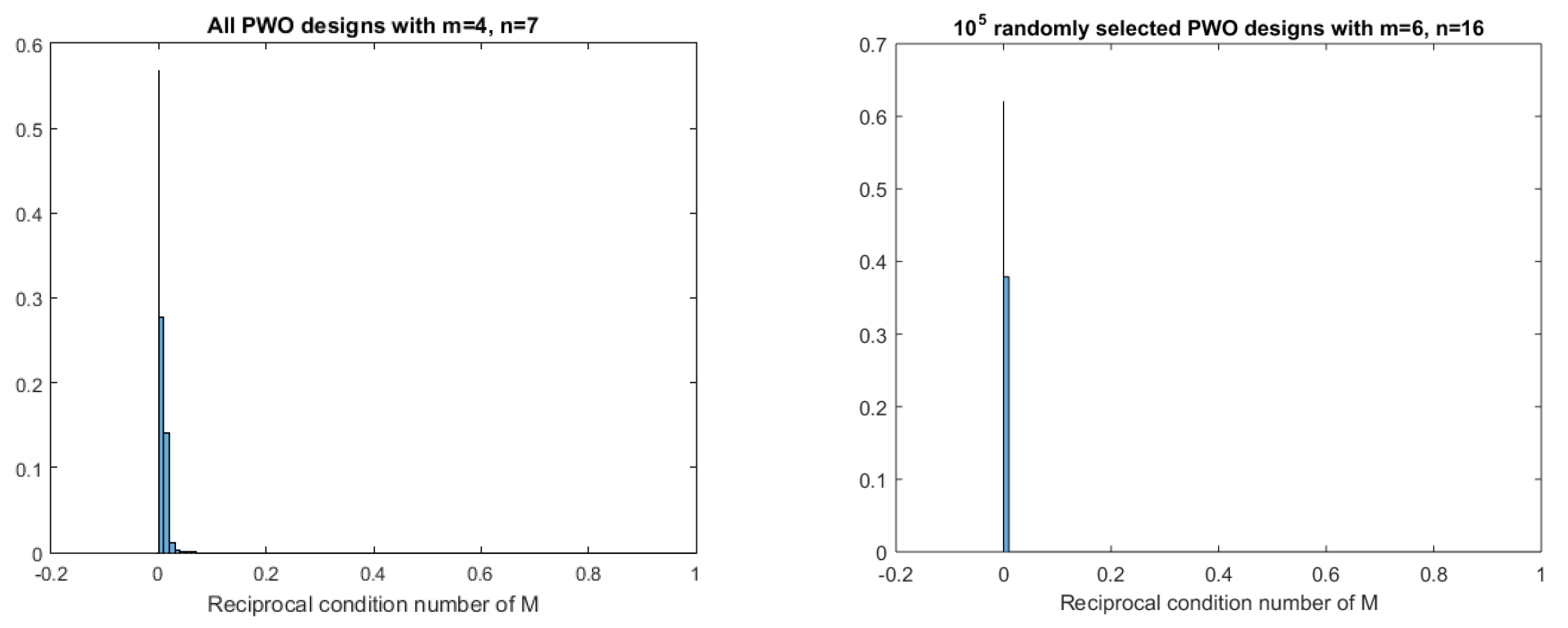
Figure 2.
D-, A- and -efficiencies of PWO designs generated initial design, and each graph contains four lines corresponding to PWO designs with components and runs, respectively.
Figure 2.
D-, A- and -efficiencies of PWO designs generated initial design, and each graph contains four lines corresponding to PWO designs with components and runs, respectively.
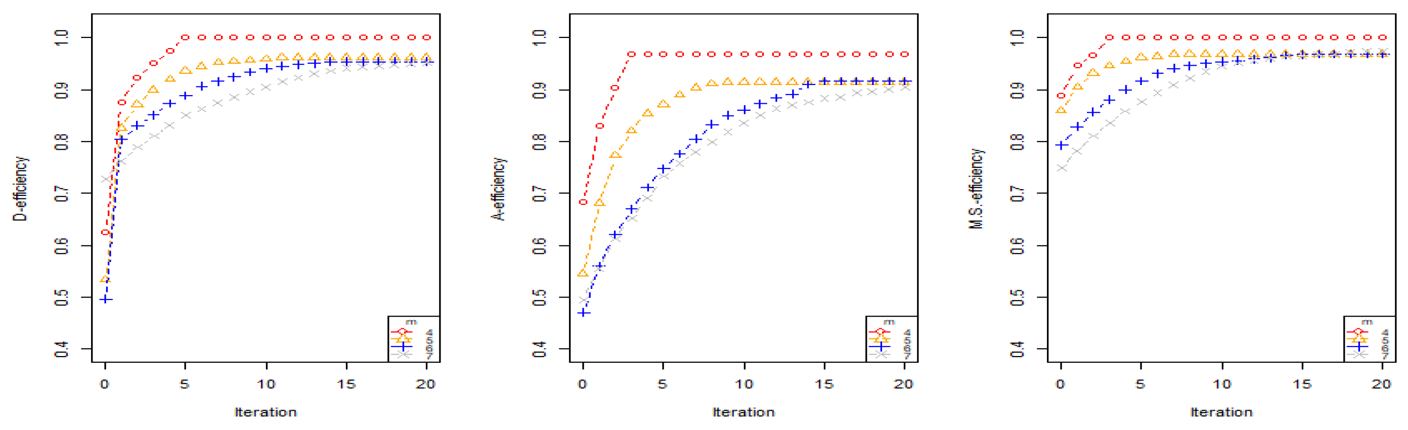
Figure 3.
Boxplot of the A-efficiencies for the Ex-PSO-A designs with components and generated by one hundred runs of Ex-PSO.
Figure 3.
Boxplot of the A-efficiencies for the Ex-PSO-A designs with components and generated by one hundred runs of Ex-PSO.
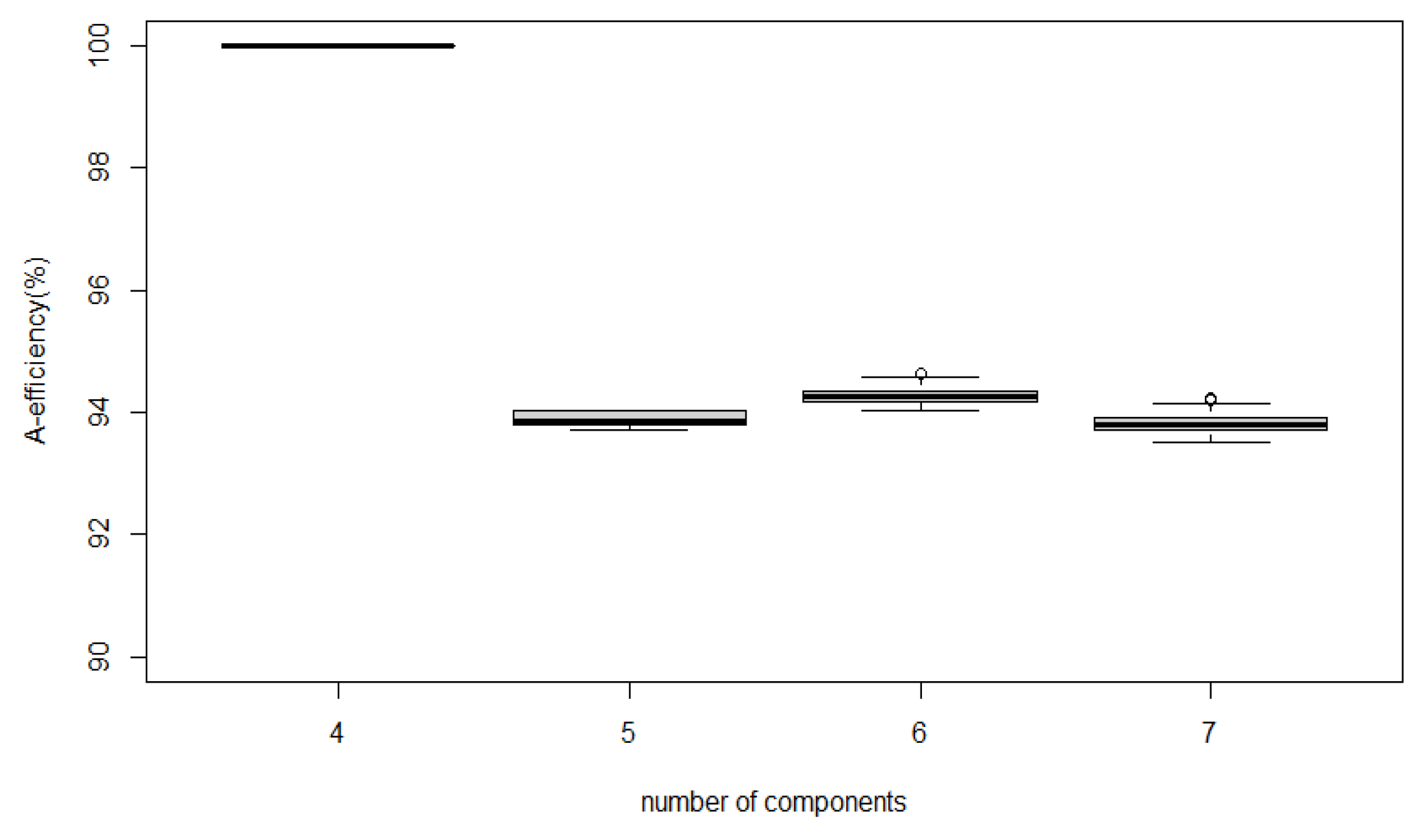
Figure 4.
Relative efficiencies of Ex-PSO designs with compared with the full PWO design for the OofA experiment with 4 components.
Figure 4.
Relative efficiencies of Ex-PSO designs with compared with the full PWO design for the OofA experiment with 4 components.
Disclaimer/Publisher’s Note: The statements, opinions and data contained in all publications are solely those of the individual author(s) and contributor(s) and not of MDPI and/or the editor(s). MDPI and/or the editor(s) disclaim responsibility for any injury to people or property resulting from any ideas, methods, instructions or products referred to in the content. |
© 2023 by the authors. Licensee MDPI, Basel, Switzerland. This article is an open access article distributed under the terms and conditions of the Creative Commons Attribution (CC BY) license (http://creativecommons.org/licenses/by/4.0/).
Copyright: This open access article is published under a Creative Commons CC BY 4.0 license, which permit the free download, distribution, and reuse, provided that the author and preprint are cited in any reuse.


