Submitted:
20 April 2023
Posted:
21 April 2023
You are already at the latest version
Abstract
As semi-airborne mineral exploration has limited budgets, it is critical to design experimental procedures that generate data maximizing the desired information We investigate the effects of transmitter-receiver geometries for a variety of anomalies and semi-airborne layouts. Our simulations indicate that 200 m flight line spacing and 100 m point distance are the optimal trade-off between coverage and survey progress for various targets. Based on the target size and distance between the transmitter and the target, the transmitter length should be at least equal to the length of the target and for more than 1 km, at least two or three times the target size. Likewise important are the location and direction of the transmitter cables, which can have great impact on the result of inversion and should be parallel to the target strike. By using more than one transmitter, better results are obtained. If the strike of the target is known, transmitters should be parallel to each other and if not, it is better to use perpendicular transmitters. Results showed that the optimal distance between transmitters is 3 km. Our simulations show that it is even possible to recover targets just below the transmitter in corresponding areas of masked data.
Keywords:
Geophysical survey
; Semi-airborne electromagnetics
; Inversion
; Mineral exploration
1. Introduction
Considering the role of minerals in providing the basic needs of various industries, it seems necessary to search for them with efficient methods. Nowadays, it is not possible to search for mineral resources only by using surface geological information. Electromagnetic geophysical methods are highly effective in searching for the mentioned sources. These methods are used in almost all stages of exploration operations, which are cheap, reliable, and in many cases reduce big investment risks. By using geophysics, it is possible to identify parts of the earth that have different physical characteristics from the surrounding environment, such as mineralized zones. The ultimate goal of all applied geophysical explorations is to achieve an accurate picture of the properties of materials below the surface of the earth. The actual structures below the Earth's surface are often very complex. Therefore, an attempt is made to provide a simpler model of the earth that is controlled by a finite number of parameters. Resistivity is among the most important geophysical parameters and used to identify and explore areas prone to mineralization. Required steps are preliminary geological investigations, data collection, and finally, interpretation. Most geophysical studies deal with mathematics governing the problem for the data processing, modelling and inversion [1,2].
An important link that has barely been addressed is the data collection itself and the related design of surveys that in the end dictates the quality of subsurface information provided by practical implementations of geophysical methods. King & Constable [3] investigated resolution and depth sensitivity in different CSEM systems. They find the tradeoffs between different systems such as nodal and towed CSEM to reach greater depth with better resolution. Maurer et al. [4] used examples from direct-current electrical and frequency-domain EM applications, with approaches to quantitative experimental design. These approaches are repeated forward modelling and the data importance function, which shows the influence of each data point on determining the final inversion. In the end, they proposed a method based on global optimization algorithms that can be customized for individual needs. Henning et al. [5] introduced a procedure to reduce the number of geoelectrical multielectrode measurements of a survey. The reduction is achieved by an optimization of the resulting sensitivity distribution using a superposition of different measurements in comparison with a target sensitivity distribution. To distinguish between important and non-important measurements, they used the absolute value of weighting factors and neglected measurements with small weights. Coscia et al. [6] designed optimized electrode configurations to employ cross-hole electrical resistivity tomography for monitoring fast hydrological processes that involve complex interactions between a river and the adjacent groundwater. Loke & Wilkinson [7] also worked on optimizing arrays for Electrical Imaging Surveys. They worked on optimizing non-traditional arrays. So that when a new set of electrodes is added to the array they can calculate model resolution changes, instead of entire resolution matrix, faster by parallel computing using GPUs. Nowruzi [8] and Ahmadi [9] investigated the theoretical and practical concepts of geometric probabilities, and presented the relations of geometric probabilities to determine the probability of the intersection of various geometric shapes with different types of grids (Buffon's needle problem). Since the geometric parameters of mineral deposits are of a probable nature, the exploration of mineral deposits is also of a probable nature and is always associated with uncertainty and some risk. Agocs [10] is one of the first that studied the effect of changing the distance of flight lines and the location of these lines in airborne surveys by using the relationships related to the probability of discovery, which are obtained based on geometric probability theories and Buffon's needle problem. McCammon [11] and Chung [12] also used this theory to study the effect of the distance of the parallel survey lines on the possibility of deposit exploration. There are other studies that have been done in other methods, for example, seismic tomography [13,14] and reflection surveys [15,16,17].
There are only very few studies on the survey design of airborne electromagnetics (AEM), especially semi-airborne EM. In the DESMEX project, Becken et al. [18] developed a new semi-airborne (EM) system with data analysis in the frequency domain. Smirnova et al. [19] studied the source parameters such as current, cable length and frequency on simple 1D models and showed how fields behave in different backgrounds for a 2 km source. They demonstrated how the field decays and goes into the noise level based on current, cable length for two different frequencies. They used 3D synthetic models to show the dependence of the response with frequency, depth, and thickness of the conductor and transmitter-receiver distance on real data. Chen & Sun [20] used layered synthetic models to investigate the characteristics of semi-airborne transient EM (SATEM) with different parameters such as flight altitude, offsets, and geometry positions and defined an ellipse equation to separate suitable and unsuitable areas for survey with SATEM system. This ellipse equation fits better to short-line sources and not long sources. Ke et al. [21] worked on multi-component 3D inversion of SATEM systems in presence of topography. They used synthetic modelling to demonstrate the importance of multi-component inversion. They first used single component 3D inversion to detect a plate in vertical and horizontal situations. Their study showed that using single-component inversion does not give good results. For example, using just the z-component, they could only detect the top of vertical plate. Then they present different complex models using multi-component inversion. In the following, we will first talk about the inversion method and then about the survey parameters involved in data collection, cost, and time.
2. Methodology
2.1. Scheme
Airborne electromagnetic (AEM) methods measure the magnetic field to calculate the resistivity distribution of the earth’s subsurface and are widely used mineral exploration and groundwater studies [22,23]. AEM surveys can cover large areas in short times and are much more efficient than ground geophysics. Most importantly, they can handle rough or even inaccessible terrain and topography. Because the power of a pure airborne transmitter is practically limited, the penetration depth of pure airborne EM is limited to a few hundred meters. However, modern exploration targets are at increasingly greater depths up to 1 km, requiring greater transmitter moments for sufficient signal-to-noise ratios. The semi-airborne EM (SAEM) method uses ground-based transmitters and airborne magnetic field receivers, as illustrated in Figure 1. This method allows the usage of powerful transmitters on the ground, whereas the advantages of survey efficiency and spatial coverage of AEM can be partially maintained when a passive sensor system is carried by aircraft in the vicinity of the transmitter cable [1]. In this study, for modelling and inversion, we used frequencies from 16 to 1024 Hz in octave steps that are similar to mid-range frequencies of the “SQUID bird” that was developed jointly by the Leibniz Institute of Photonic Technology and Supracon AG, Jena, Germany [24,25].
2.2. Forward problem and Inversion
We solve the total-field formulation of the Maxwell equations (Eq 1) based on accurate second order finite element forward operator with the open-source toolbox custEM [26]
where the ω is the angular frequency, σ the electric conductivity, and je the source-current density. custEM implements a finite-element discretization on unstructured meshes and Nédélec basis functions in collaboration with the direct solver MUMPS. The time-harmonic curl-curl equation for the electric field with the common quasi-static approximation for the frequency range of CSEM methods reads. Finally, we solve a linear system of equations AE=b for each frequency and calculate the magnetic field using equation 2 [26,27].
Most recently, Rochlitz [28] presented a new inversion workflow based on the pyGIMLi [29] framework, which solves equation 3 with a least-squares conjugate gradient solver [30] avoiding any matrix-matrix multiplication.
where J is the Jacobian matrix containing sensitivities of N data observations d to M model parameters m (the logarithmized conductivities), f(m) is the forward response of the model m, Wd is the error-weighting matrix with inverse errors, and Wm is the smoothness operator. The inverse solver also involves the model and data transformations, whose inner derivatives are used to scale the model, data and the Jacobian matrix. We use a two-sided logarithmic transformation [28] to constrain the resistivity between and Ωm (Eq 4).
In addition to performance and convenience improvements, custEM includes sub-modules for explicit Jacobian calculations and a communication interface with pyGIMLi's inverse solver. All vectors are assembled only locally on cells, avoiding equivalent vector derivative expressions for system matrix derivatives. Various shapes of receiver patches with individual field components and transmitter relationships allow grouping electric- and magnetic field data sets without memory or computation overhead. Additionally, we eliminate unnecessary back-substitutions for masked data, i.e., below the noise level [28].
3.4. Synthetic experiments
For the experimental design, we have conducted synthetic experiments using a relatively simple model of a conducting block in a resistive background. The resistivity of the block and background are 1 and 300 m. Gaussian noise has been added to the data and the regularization parameter was selected such that the data are fit within the noise level and have a smoother result. As error model (standard deviation of the noise and inverse weighting) we used a relative error of 5% and an optimistic absolute error level of 1 pT/A. The flight altitude is 50 m above the ground. The receivers cover an area of around 10 km2 (3×3.2 km).
Due to the fact that the field is very strong at the location of the transmitter and decays rapidly near the transmitter, in many cases, the data surveyed on or near the transmitter cannot be used for inversion because they can cause artificial effects and mask the anomalies [26,32]. In these cases, we do not consider the data up to a certain distance from the transmitter, in our case, 400 m, and remove data around the transmitter.
3. Single and Multi-component inversion
The synthetic model consists of a block with dimensions of 200×1000×500 m buried at 150 m from the ground level. Figure 1 displays a sketch of this model.. In this model, the transmitter is a two-km-long cable that is placed parallel to the block strike. Figure 2 shows the inversion results with subfigures a,b,c, and d are the case of a single component inversion and subfigures a and b are the x-component results. Resistivity distribution is better describing the edges of the body in the x direction. Anomaly of the body less inclined towards the transmitter but on the other hand effect of the body reach the surface. In the same way in subfigures c and d (z-component result), the resistivity is more limited to the edges in z direction but more tends towards the transmitter. We can recover the body properly with lower resistivity resolution. Subfigures e and f shows that, with using multi-component inversion the block edges are better recovered in all directions and, moreover, the maximum resistivity values are higher. Our results are in agreement with Ke et al. [21] studying multi-component inversion. As a result, all other modellings you will see in the following are multi-component inversion results.
4. Survey parameters
4.1. Surveying grid size (data density)
With point and line spacing parameter we examined the effect of data point density on the result of inversion, number of flight lines or cost. Table 1 shows the variables of this modeling.
Figure 3 shows the results. Subfigures a,b are the results for 100×100 m survey grid and we can see better result that is closer to the body properties or higher resolution, but takes 19 hours to run. Subfigures c,d are the 200×100 m grid size that gives a reasonable result with respect to the run time and resolution. Most importantly, in this case, flight lines are half of the 100×100m grid and this means less costs. The subfigures e,f are the 200×200 m result that are lower in resolution. Based on the results of the inversions with different grid sizes. The more the flight lines spacing increases and therefore the number of data points decreases, the lower the resolution becomes. However, a denser flight line spacing increases the number of flight lines and more data points increase inversion time, as Table 1 shows by the factor of 2 or 3. Therefore, we used 200×100 m data spacing for modelling in this study because it is faster to run and needs less flight lines in survey.
4.2. Transmitter length
In this step, we examine the effect of the transmitter length. We consider the same model for this, but this time the block is located at 50m depth. It is worth mentioning that we could use a really long transmitter like 10 km or more, but we consider practical limitations of the transmitter layout for real surveys. Therefore, the objective is to achieve a good trade-off between resolution and installation effort. Starting with the block 1 km from the transmitter, the transmitter length increases from 1 km to 3 km. In this case, the block is close to the transmitter and as a result, the signal is strong at the block. Figure 4a indicates that using a transmitter length of at least equal to the length of the target provides a good target recovery. For obtaining a good result with higher resolution, it is better to use a transmitter with twice the length of the target (Figure 4c).
Next, we put the block 2 km away from the transmitter, and at this distance, the signal is weaker in comparison with the previous model (Figure A1). Again, transmitter length changes from 1 km to 3 km. We can see in Figure 4b that 1 km transmitter does not produce a strong enough primary field at the block. As result resolution is weak. Transmitter with twice the length of the target block gives fair result (Figure 4d) and using a transmitter three times the length of the target (Figure 4f) gives a better result in this distance. In this situation it is better to use a transmitter with three times the length of the target.
In the last model the block is at 3 km from Transmitter, in this situation signal at the block location is weak (Figure 5). Figure 5a shows that with 1 km transmitter, we can’t see the block at all because of the weak signal at that distance. Using the 2 and 3 km length transmitter doesn’t give reasonable results (subfigures 5b, 5c), we even used a 4 km transmitter, but the results are just slightly better in resolution (Figure 5d). Another important point here is that even with a long transmitter such as 4 km, the maximum distance that we can rely on the data is 3 km from the transmitter. We recommend that for long distances it is better to use transmitters with at least four times the length of the target.
4.3. Transmitter orientation with respect to the block
In many cases of mineral exploration, there is at least some geological and geometric information on the target based on preliminary studies. In this situation, we have some general knowledge of the target, and it is the best-case scenario because we know we should lay down the transmitter cable parallel to the main strike of the target to have the best coupling of the transmitter and target. To demonstrate this, we assume the same model as in the previous section. Figure 4c shows that the best results are obtained when the target is closer to the transmitter (1 km) and the transmitter length is twice the length of the target. This time we laid down the cable perpendicular to the body. Figure 6a shows that, in this model the block strikes perpendicular to the transmitter. In this situation even when the right side of the block is only located 500m from the transmitter, the results are not good. we can’t recover the body boundaries but just front of the body. In Figure 6b the conductive body is 2km away from the transmitter and we can’t even see the front of the body in good resolution. This examination shows the importance of doing geological studies to obtain information on the target geometry before designing the survey.
4.4. Using more than one transmitter
In the previous modellings, we used only one transmitter. By looking closely at the results (Figure 3b,d,f), the anomaly tends toward the transmitter and this can mislead the interpretation. For example, we can lose the symmetry of the target. Another consequence of using only one transmitter is that if a conductive body is located behind the front body, it can mask by the front body (Figure 7a). A significant decay happens in the field after the front body, and this causes a loss of accuracy in the interpretation behind the block. To overcome these problems, it is better to use more than one transmitter on both sides. Figure 7b shows that with using two transmitter, both blocks are recovered in good resolution and we can distinguish them. In next steps we will see the results of doing this even in greater depths of 300 m. Using multiple transmitters helps to improve resolution at greater depths. Therefore, it is important to use more than one transmitter. In the next steps we will talk about how to use these transmitters in terms of their orientation and distance.
4.5. Transmitter orientation with respect to each other
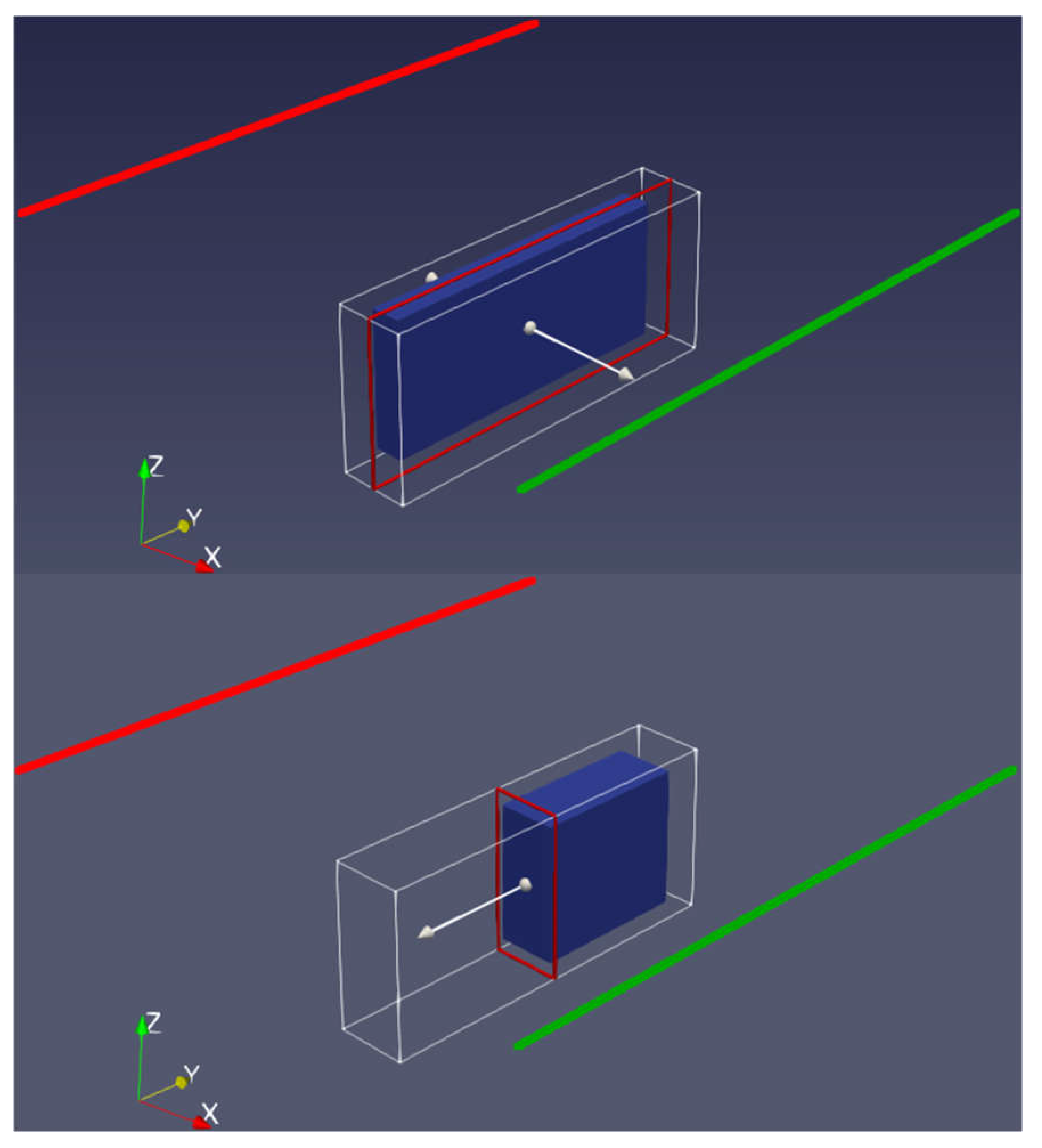
In previous models, we assumed to know the general strike of the target and we laid down the Tx cable parallel and also perpendicular to it. The results showed that the parallel configuration is much better. If we don’t know the target geometry, one reasonable idea is to use more than one transmitter in a way that the transmitters are perpendicular to each other. A sketch of such a model is presented in Figure A2 in the Appendix. Figure 8 shows the results using the perpendicular layout. The body was recovered much better with higher resolution and the resistivity distribution is more limited to the body. To prove this design method, we considered a more complex model that includes a dipping plate with dimensions of 100x500x100 m, a dip angle of 45 degrees and an azimuth of 45 degrees. The centre of the plate is located at a depth of 300 m from the surface of the earth. Figure 9a shows front view and 9b side view of the plate inversion. Plate recovered with good resolution so that resistivity distribution follows the plate geometry. In the absence of information about the target, it is better to use at least two perpendicular transmitters. From a logistic point of view (i.e. the installation of grounding points), it is better if one end of the transmitters is close to each other or use the same grounding station at the same end (Figure A2 in the Appendix).
4.6. The distance of the transmitters from each other
In case we have general information on the target, we can use parallel transmitters on both sides of the target. Now we investigate the optimal distance between these two transmitters and how this distance affects the depth of investigation. We considered a model that includes a block at different depths of 150, 300, and 500 m from the surface of the earth. Two transmitters are considered parallel to this block. The geometry of this model is presented in Appendix Figure A4, which are located at a distance of 2, 3, and 4 km from each other.
First, we investigated the case when the transmitter distance is 2 km. Figure 10a shows the result for a body located at 150m depth. The body is recovered with high resolution so that resistivity distribution is more limited to the edges. We can see the geometry or edges of the target better. In the same way, Figures 10d and g shows the results for body located at depths 300 and 500 m. As the body moves towards depth, the resolution decreases but still we can detect it. This means that by using 2 km distance between transmitters we can detect targets up to 1 km depth.
For further investigation and to achieve the optimal distance, the distance between transmitters changed to 3 and 4 km. Figure 10b shows that, for the block near surface (150m) and in the case where the distance between the transmitters is around three km, it is still possible to determine the location of the block. But Figure 10c shows with 4 km distance between the transmitters, the resistivity distribution moves toward the surface, but we can still see the body with lower resolution. When the same block goes to a depth of 300 m, we can detect it with acceptable resolution using 3 km distance between the transmitters (Figure 10e). Figure 10f shows using 4 km distance between the transmitters body recovered with low resolution.
Figure 10g, h and i shows the results for body located at 500 m depth. Based on Figure 10h when the distance between the transmitters is three km, we can recover the body with low resolution. But Figure 10i shows for a distance of 4 km it is practically impossible to detect the boundaries or location of the block.
The results show that the closer the transmitters, the better the results are (Figures 10a, d, and g), but this proximity causes a smaller area to be covered per helicopter flight resulting in more flights and thus increased costs. As a result, the optimal distance between two transmitters in this case for exploration up to a maximum depth of 1 km is 3 km (Figures 10b, e, and h). It is important to note that the length of the transmitter is 2 km, which is close to the average length of the surveys done by the LIAG [19,28]. Of course, you can use a transmitter of any length, but the limitations of the real field do not allow it in most cases.
4.7. Anomalies under the transmitter
As mentioned before, we do not consider the data points up to a certain distance from the transmitter, typically 400 m [28,32]. By considering a respective model as before, we removed the data around the transmitter up to a distance of 400 m from each side. The results showed that in this case, when the block is located at a depth of 150 m below the transmitter, it is recovered well (Figures 11a and b). In the second case, when the block is placed at a depth of 300 m, it is relatively well recovered (Figures 11c and d), but when it goes to a depth of 500 m, it becomes difficult to identify its location (Figure 11e and f). As explained in the previous section, it is better to use two transmitters, and with this method, we can use one of the transmitters to cover the data near the other one, which helps to estimate the depth of the investigation and the better resolution of the results. Figure 12 shows, covering the masked data point with another transmitter helps imaging the block at 500 m depth with higher resolution, compared to one transmitter. We conclude that we can still recover an anomaly underneath the Transmitter without data points located exactly on top of the body.
5. Discussion
We used synthetic modelling and inversion to examine how different field survey parameters affect the inversion results and to optimize them. At first, we showed the importance of multicomponent inversion .Using all three components increases the accuracy in recovering the resistivity of the body and its boundaries. Our results are in agreement with Ke et al. [21]. The number of flight lines is one of the most important factors affecting the cost of the survey. In general, denser lines lead to a better data coverage, which suggest a steadly increasing resolution of inversion.However, depending on the target size and geometry, there is a reasonable limit of data density to recover conductive bodies well. Collecting more data hardly increases the resolution anymore and only produces additional survey costs as well asprocessing and inversion runtimes. By examining different models, we concluded that a line spacing of 200 m with 100 m in-line spacing provides the otimal trade-off between cost and resolution.
The longer the transmitter is, the stronger the signal will be. However, the installation of the transmitter, including finding suitable grounding locations and laying out cables, is strongly controlled by the field conditions. The models showed that in general, if the distance between the transmitter and the target is 1 km, the minimum length of the transmitter should be at least equal to the largest target dimension. For better results, it should be twice the target dimension. If the target is located within 2 km of the transmitter, the minimum length of the transmitter should be three times the length of the target, and if the target is within 3 km, a transmitter with a length of at least four times is needed. Figure A1 shows that the signal becomes extremely weak and unreliable after three km and goes below the typical noise level.
An important issue to be considered before installing the transmitter is its orientation relative to the target geometry. In this case, it is necessary to use geological studies before geophysical surveying to determine the general strike of the target and install the cable parallel to it to obtain the highest coupling. Results showed that the transmitter orientation has a great impact on the inversion result. If the cable is roughly perpendicular to the target, it is difficult to image the whole target (Figure 6). We also showed that if one body is placed behind another, it is be difficult to distinguish both or even to detect the further as it is masked by the first (Figure 7). As a result, we suggest using more than one transmitter. When having information about the strike direction, two transmitters should be installed parallel on both sides of the target, with the optimal distance of 3 km assuming 2 km transmitter lengths (Figure 7&Figure 10). If the information about the strike direction is limited, the best method is to use transmitters with different orientations depending on local conditions (Figure 8&Figure 9). Finally, our studies showed that even if data are removed in a certain distance from the transmitter, the body under the transmitter can still be recovered. In case of larger target depths, it is nevertheless suggested to use multiple transmitters for improving the resolution at depth.
The main reason for using a semi-airborne EM system is to cover wide areas in short time with superior signal to-noise ratios compared to pure airborne EM systems. Furthermore, airborne methods in general help to work in arbitrary topography, e.g. impassable or rough terrain. Our study tried to find general rules to optimize the trade-off between resolution and costs. Summarizing the individual survey parameters and arguments discussed previously, we suggest a survey layout scheme by using eight main transmitters with lengths of 2 to 3 km (Figure 13). For this design with overlapping injection points, we need only nine grounding positions (using main transmitters only) instead of 16 used for eight separated transmitters, which means less logistic effort. Here, six of the transmitters are parallel to each other and two others are perpendicular. With this layout, we are minimizing the number of perpendicular transmitters to two only. As we showed before, this approach helps to image the subsurface with a much higher resolution. This layout can cover an area of 36 km2 with high resolution (inside of the 2x2 transmitter square) and a total area of 84 km2 (outside). The optional transmitters (green lines) will further improve resolution, particularly in cases of unknown strike direction, and increase the area to 144 km2. Note that this scheme can be arbitrarily extended to larger survey areas by moving the transmitter combination by steps of 3 km in all directions.
We used comparatively simple models in terms of conductivity and geometry. For future studies, we suggest moving toward more realistic geological settings for addressing goals in real mineral exploration. One of the most important features of the real world is topography. In the present of topography, sometimes helicopters need to fly at higher altitude, which means larger offsets. Motional noise can affect the data processing and extracting x, y, and z components. One of the interesting future studies can be using the total magnetic field vector in terms of Amplitude and Phase for the inversion. Using different error models also should be studied. In this study, we used 7 frequencies from 16 to 1024 that is a limited range of frequencies for our modelling and suggest using lower and higher frequencies to examine the outcome.
6. Conclusions
Our experiments show that multi-component inversion is very important, particularly in complex survey areas. Since many mineral deposits are embedded in complex geological structures, we suggest relying on systems with multi-component surveying capabilities which became increasingly available in recent years. The exploration stage is one of the most expensive stages in mineral economics. Our modelling suggests 200 m flight line spacing to reduce the survey costs while obtaining reliable results at the same time. Data gaps in the vicinity of transmitters do not significantly limit the resolution capabilities just below the transmitters. Very long transmitters produce the strongest signals, but in reality, the length of the transmitter is often controlled by the field conditions. We suggest using multiple transmitters with a length of 2 to 3 km, which produce sufficient signal quality up to distances of 3 km. By using appropriate geological studies before designing survey plans, the mineralization type and strike can be determined to some extent. A parallel transmitter layout according to this information maximizes the target resolution capabilities. To get an even better image of the targets, we recommend two parallel transmitters at 3 km distance on both sides. In cases where mineralization is very complex so that it is impossible to detect its strike, several perpendicular transmitters should be used. Finally, we presented a general scheme that is very suitable for covering large areas for simultaneously obtaining maximum information at an optimal cost.
Author Contributions
Conceptualization and methodology, T.G. and S.N.; software, R.R. and T.G.; formal analysis, S.N.; writing—original draft preparation, S.N.; writing—review and editing, R.R. and T.G.; visualization, S.N. and T.G.; project administration and funding acquisition, T.G.; All authors have read and agreed to the published version of the manuscript.
Funding
The paper is financially supported by the Federal Ministry of Education and Research (BMBF) of Germany under grant numbers 033R385D and 033R130DN.
Conflicts of Interest
The authors declare no conflict of interest.
Appendix A
Figure A1.
Synthetic data of one flight line over a homogeneous half space 300 Ωm. Frequency is 512 Hz. a. data without noise b. noisy data.
Figure A1.
Synthetic data of one flight line over a homogeneous half space 300 Ωm. Frequency is 512 Hz. a. data without noise b. noisy data.
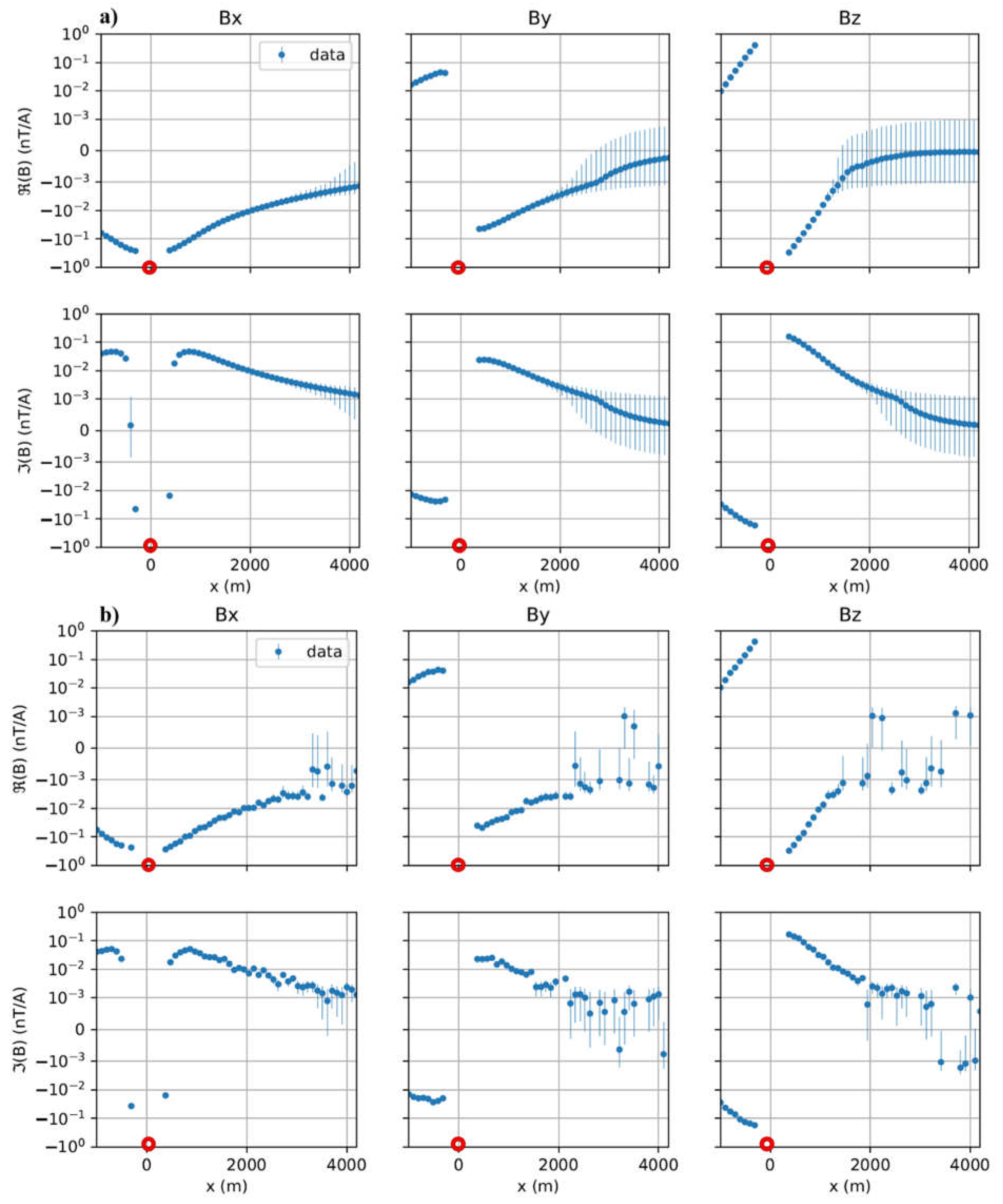
Figure A2.
Sketch of the model using two transmitters perpendicular to each other. Red line is the Transmitter one and Green line is Transmitter two.
Figure A2.
Sketch of the model using two transmitters perpendicular to each other. Red line is the Transmitter one and Green line is Transmitter two.
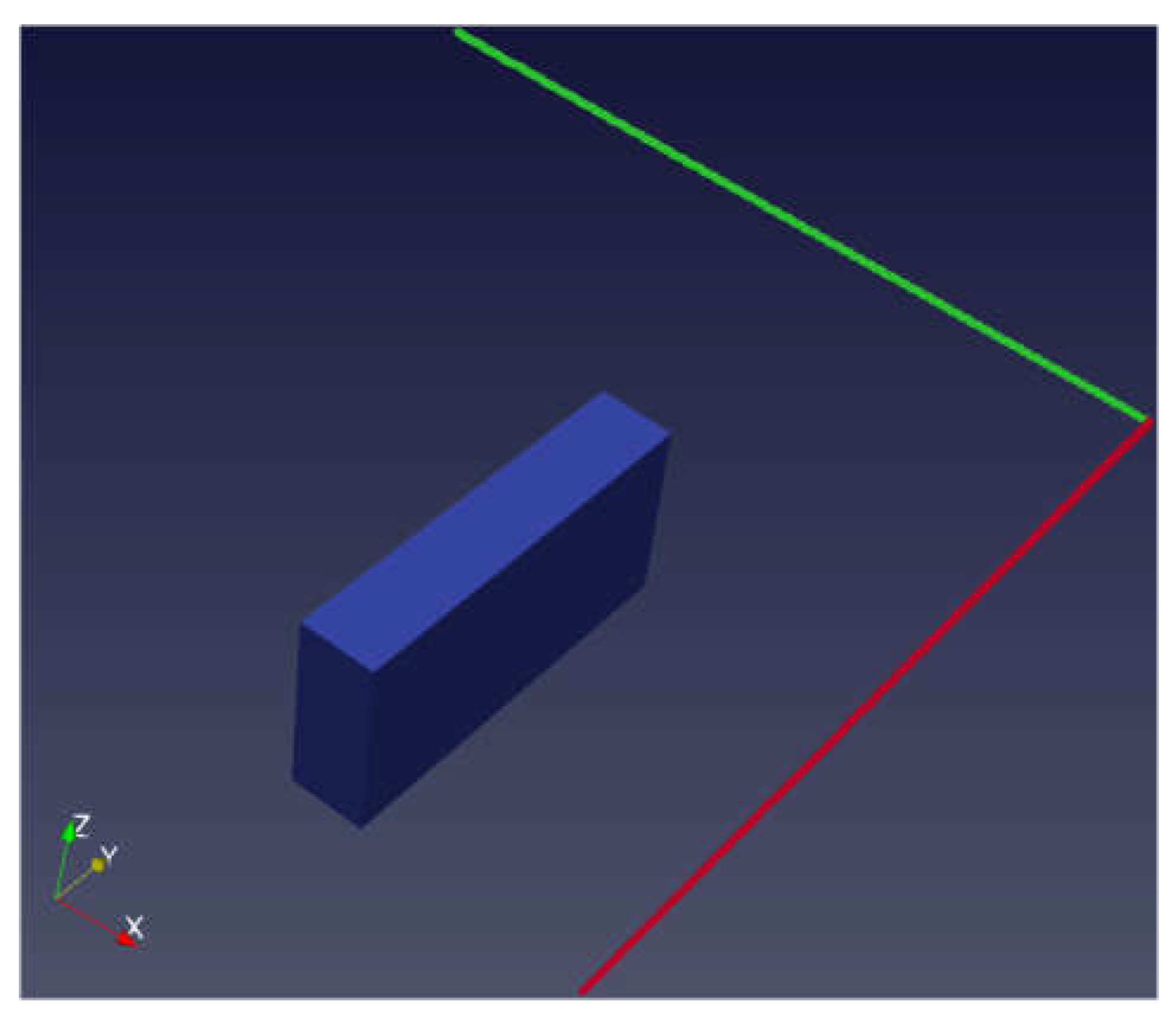
Figure A3.
Sketch of the dipping plate using two transmitters perpendicular to each other. Plane views are 45 degrees in xy plane. Red line is Transmitter 1 and Green line is Transmitter 2.
Figure A3.
Sketch of the dipping plate using two transmitters perpendicular to each other. Plane views are 45 degrees in xy plane. Red line is Transmitter 1 and Green line is Transmitter 2.
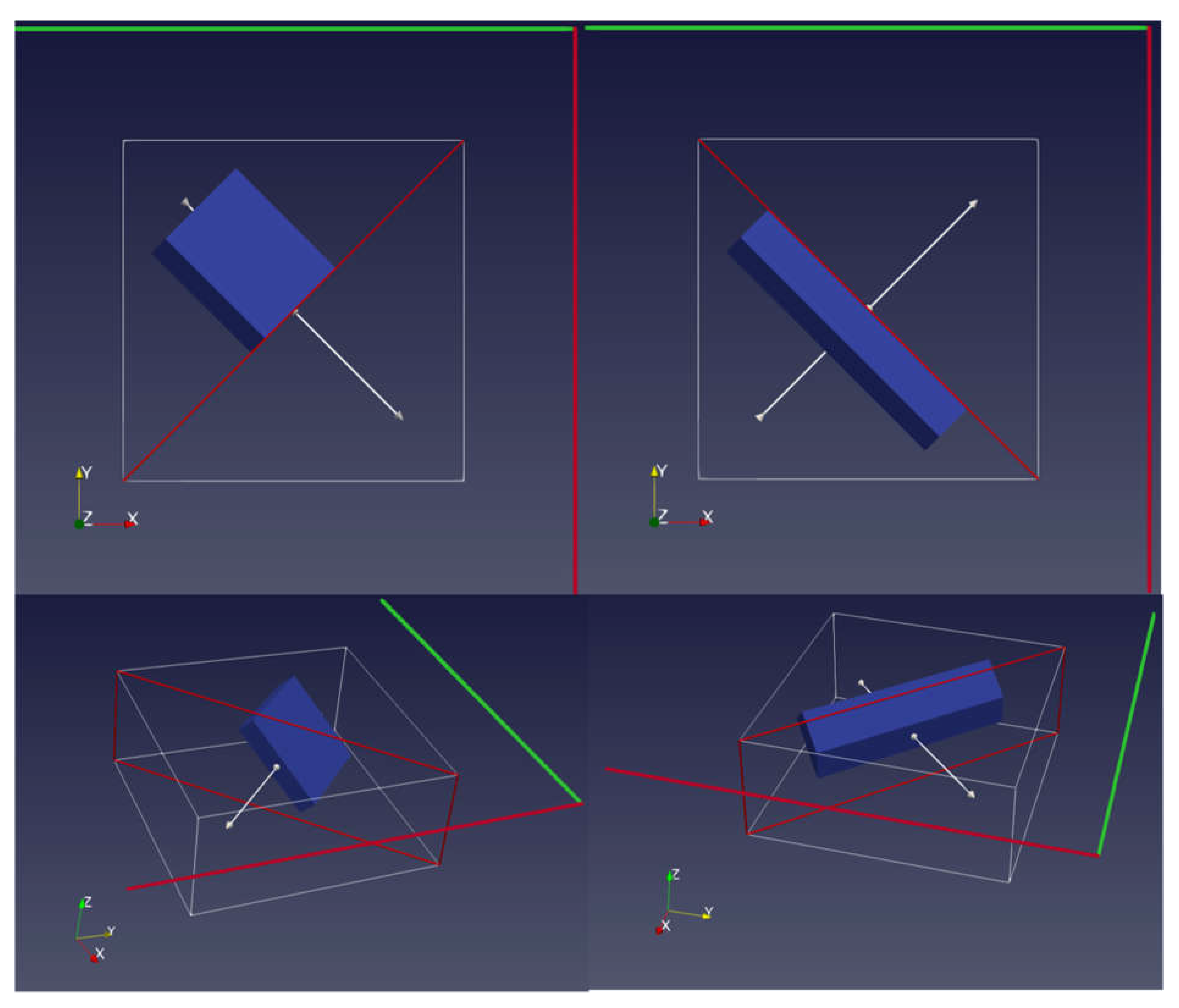
Figure A4.
Sketch of the model using two transmitter parallel to each other. Red line is the Transmitter 1 and Green line is Transmitter 2.
Figure A4.
Sketch of the model using two transmitter parallel to each other. Red line is the Transmitter 1 and Green line is Transmitter 2.
References
- Kearey P, Brooks M, Hill I. An introduction to geophysical exploration. John Wiley & Sons; 2002 Apr 26.
- Dentith M, Mudge ST. Geophysics for the mineral exploration geoscientist. Cambridge University Press; 2014 Apr 24.
- King, R. B., & Constable, S. How low can you go: An investigation of depth sensitivity and resolution using towed marine CSEM systems. Geophysical Prospecting 2023. [CrossRef]
- Maurer, H., Boerner, D. E., & Curtis, A. Design strategies for electromagnetic geophysical surveys. Inverse Problems 2000, 16(5), 1097. [CrossRef]
- Hennig, T., Weller, A., & Möller, M. Object orientated focussing of geoelectrical multielectrode measurements. Journal of Applied Geophysics 2008, 65(2), 57-64. [CrossRef]
- Coscia, I., Marescot, L., Maurer, H., Greenhalgh, S., & Linde, N. Experimental design for crosshole electrical resistivity tomography data sets. Ext. Abstr. Near Surface 2008-14th EAGE European Meeting of Environmental and Engineering Geophysics 2008. 64. EAGE Publications BV. [CrossRef]
- Loke, M. H., & Wilkinson, P. (2009, September). Rapid parallel computation of optimized arrays for electrical imaging surveys. Ext. Abstr. Near Surface 2009-15th EAGE European Meeting of Environmental and Engineering Geophysics 2009. 134. EAGE Publications BV. [CrossRef]
- Nowruzi, GH. Optimum design of survey grid in magnetic studies. University College of Engineering 1997, 30(2), Tehran.
- Ahmadi, R. Application of geometric probability to design exploration grid of mineral deposits, case study: porphyry copper index located in the south-west of Kerman. Journal of Analytical and Numerical Methods in Mining Engineering 2018, 8(15), 39-54.
- Agocs, W.B. Line spacing effect and determination of optimum spacing illustrated by Marmora, Ontario magnetic anomaly, Geophysics 1955, 20 (4), 871-885. [CrossRef]
- McCammon, R.B. Target intersection probabilities for parallel line and continuous grid types of search. Journal of Mathematical Geology 1977, 9 (4), 369–382. [CrossRef]
- Chung, C. F. Application of the Buffon needle problem and its extensions to parallel-line search sampling scheme. Journal of the International Association for Mathematical Geology 1981, 13, 371-390. [CrossRef]
- Ajo-Franklin, J. B. Optimal experiment design for time-lapse traveltime tomography. Geophysics 2009, 74(4), Q27-Q40. [CrossRef]
- Brenders, A. J., & Pratt, R. G. Waveform tomography of marine seismic data: What can limited offset offer?. In 2007 SEG Annual Meeting 2007. OnePetro.
- Curtis, A., & Snieder, R. Reconditioning inverse problems using the genetic algorithm and revised parameterization. Geophysics 1997, 62(5), 1524-1532. [CrossRef]
- Liner, C. L., Underwood, W. D., & Gobeli, R. 3-D seismic survey design as an optimization problem. The Leading Edge 1999, 18(9), 1054-1060. [CrossRef]
- Sirgue, L., & Pratt, R. G. Efficient waveform inversion and imaging: A strategy for selecting temporal frequencies. Geophysics 2004, 69(1), 231-248. [CrossRef]
- Becken, M., Nittinger, C. G., Smirnova, M., Steuer, A., Martin, T., Petersen, H., ... & DESMEX Working Group. DESMEX: A novel system development for semi-airborne electromagnetic exploration. Geophysics 2008, 85(6), E253-E267. [CrossRef]
- Smirnova, M. V., Becken, M., Nittinger, C., Yogeshwar, P., Mörbe, W., Rochlitz, R., Steuer, A., Costabel, S., Smirnov, M. & DESMEX Working Group. A novel semiairborne frequency-domain controlled-source electromagnetic system: Three-dimensional inversion of semiairborne data from the flight experiment over an ancient mining area near Schleiz, Germany. Geophysics 2019, 84(5), E281-E292. [CrossRef]
- Chen, C., & Sun, H. Characteristic analysis and optimal survey area definition for semi-airborne transient electromagnetics. Journal of Applied Geophysics 2020, 180, 104134. [CrossRef]
- Ke, Z., Liu, Y., Su, Y., Wang, L., Zhang, B., Ren, X. & Ma, X. Three-Dimensional Inversion of Multi-Component Semi-Airborne Electromagnetic Data in an Undulating Terrain for Mineral Exploration. Minerals 2023, 13(2), 230. [CrossRef]
- Siemon, B., Christiansen, A.V., & Auken, E. A review of helicopter-borne electromagnetic methods for groundwater exploration. Near Surface Geophysics 2009, 7(5-6), 629-646. [CrossRef]
- Smith, R. Electromagnetic induction methods in mining geophysics from 2008 to 2012. Surveys in Geophysics 2014, 35, 123-156. [CrossRef]
- Stolz, R., Zakosarenko, V., Schulz, M., Chwala, A., Fritzsch, L., Meyer, H. G., & Köstlin, E. O. Magnetic full-tensor SQUID gradiometer system for geophysical applications. The Leading Edge 2006, 25(2), 178-180. [CrossRef]
- Rudd, J., Chubak, G., Larnier, H., Stolz, R., Schiffler, M., Zakosarenko, V., ... & Meyer, M. Commercial operation of a SQUID-based airborne magnetic gradiometer. The Leading Edge 2022, 41(7), 486-492. [CrossRef]
- Rochlitz, R., Skibbe, N., & Günther, T. custEM: Customizable finite-element simulation of complex controlled-source electromagnetic data. Geophysics 2019, 84(2), F17-F33. [CrossRef]
- Rochlitz, R. Analysis and open-source Implementation of Finite Element Modeling techniques for Controlled-Source Electromagnetics, Ph.D. thesis, Westfälische Wilhelms-Universität Münster, 2020.
- Rochlitz, R., Becken, M., & Günther, T. Three-dimensional inversion of semi-airborne electromagnetic data with a second-order finite-element forward solver. Geophysical Journal International 2023, 234(1), 528-545. [CrossRef]
- Rücker, C., Günther, T., & Wagner, F. M. pyGIMLi: An open-source library for modelling and inversion in geophysics. Computers & Geosciences 2017, 109, 106-123. [CrossRef]
- Günther, T., Rücker, C., & Spitzer, K. Three-dimensional modelling and inversion of DC resistivity data incorporating topography—II. Inversion. Geophysical Journal International 2006, 166(2), 506-517. [CrossRef]
- Kim, H. J., & Kim, Y. A unified transformation function for lower and upper bounding constraints on model parameter in electrical and electromagnetic inversion. Journal of Geophysics and Engineering 2011, 8(1), 21-26. [CrossRef]
- Steuer, A., Smirnova, M., Becken, M., Schiffler, M., Günther, T., Rochlitz, R., ... & Müller, F. Comparison of novel semi-airborne electromagnetic data with multi-scale geophysical, petrophysical and geological data from Schleiz, Germany. Journal of Applied Geophysics 2020, 182, 104172. [CrossRef]
Figure 1.
Sketch of the 3D SAEM model. White points are receivers (50 m in the air), red line is the ground transmitter. Data points are removed within 400 m distance from the Transmitter. The resistivities of the block and background are 1 and 300 m.
Figure 1.
Sketch of the 3D SAEM model. White points are receivers (50 m in the air), red line is the ground transmitter. Data points are removed within 400 m distance from the Transmitter. The resistivities of the block and background are 1 and 300 m.
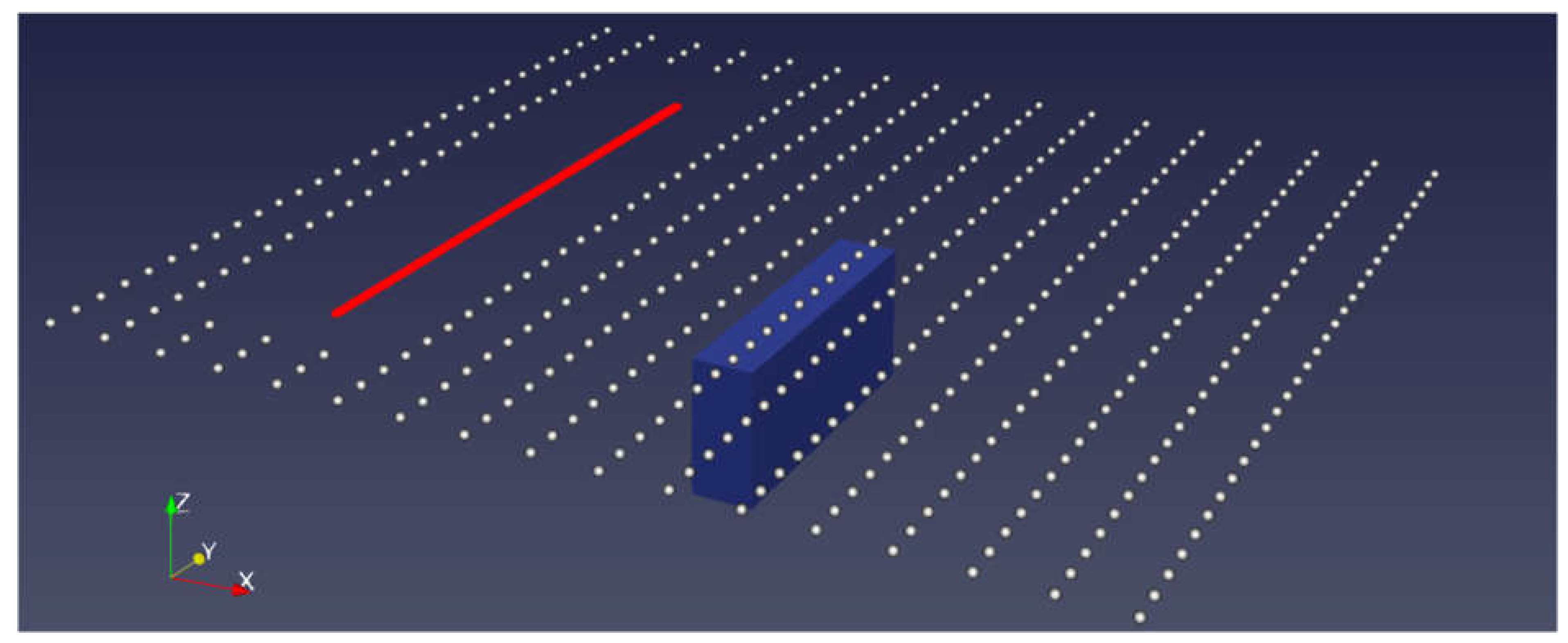
Figure 2.
Cross-sections (y-z and x-z planes) of inversion results for different components: a, b. x-component, c, d. z-component, e, f. xyz (multi)-component. In all the figures of this article, when the transmitter is perpendicular to the plane, it is shown as a red circle whereas it is shown as a red straight line when parallel to the plane. .
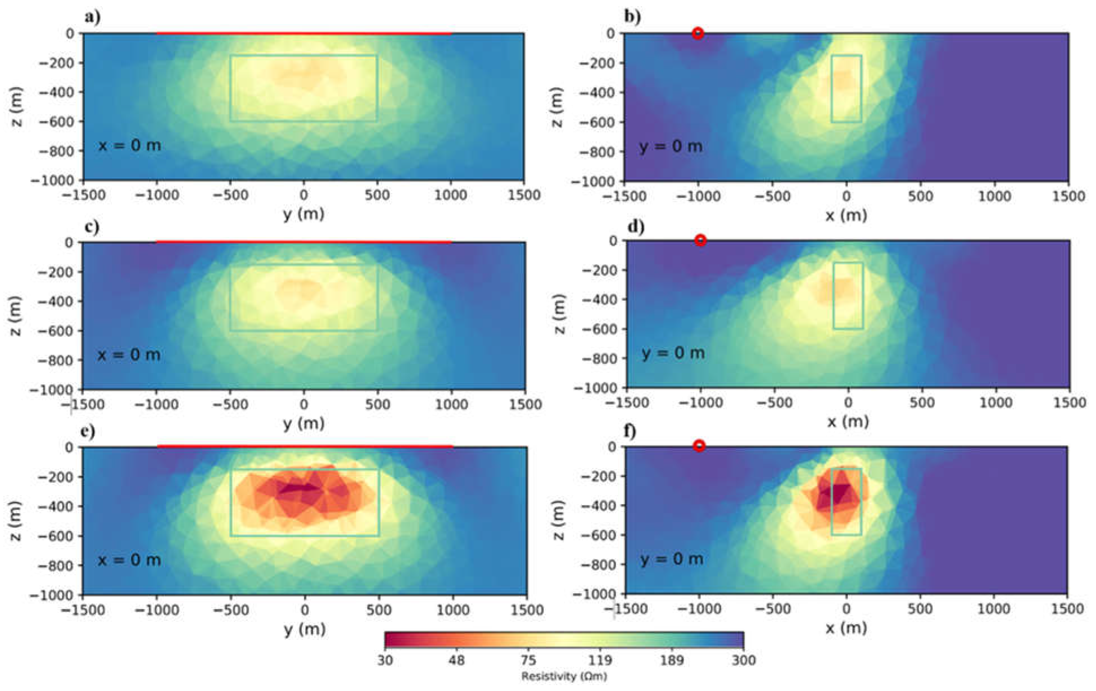
Figure 3.
Inversion results for different measuring grid sizes: a,b. 100×100 m c,d. 200×100 m e,f. 200×200 m. Blue dots are receiver positions.
Figure 3.
Inversion results for different measuring grid sizes: a,b. 100×100 m c,d. 200×100 m e,f. 200×200 m. Blue dots are receiver positions.
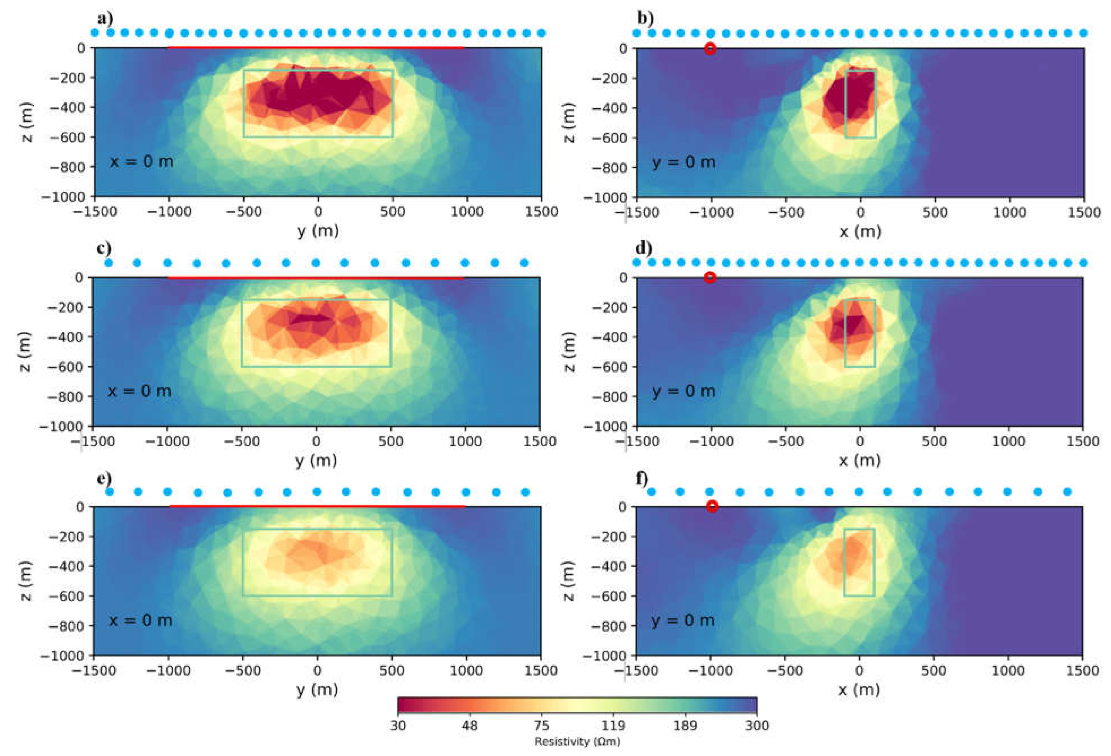
Figure 4.
Inversion results for different transmitter lengths a,b. 1 km. c,d. 2 km. e,f. 3 km. The conductive body is located a,c,e. 1 km from the transmitter. b,d,f. 2 km from the transmitter.
Figure 4.
Inversion results for different transmitter lengths a,b. 1 km. c,d. 2 km. e,f. 3 km. The conductive body is located a,c,e. 1 km from the transmitter. b,d,f. 2 km from the transmitter.
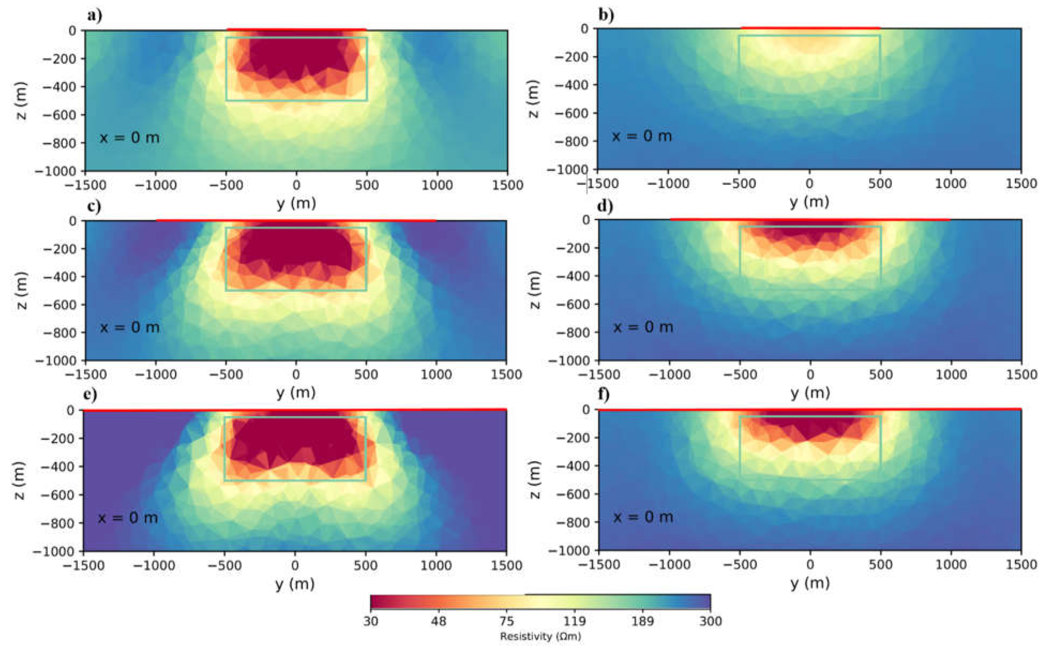
Figure 5.
Inversion results for different transmitter lengths (a 1 km, b 2 km, c 3 km, d 4 km), in this case conductive body located 3 km away from the transmitter.
Figure 5.
Inversion results for different transmitter lengths (a 1 km, b 2 km, c 3 km, d 4 km), in this case conductive body located 3 km away from the transmitter.
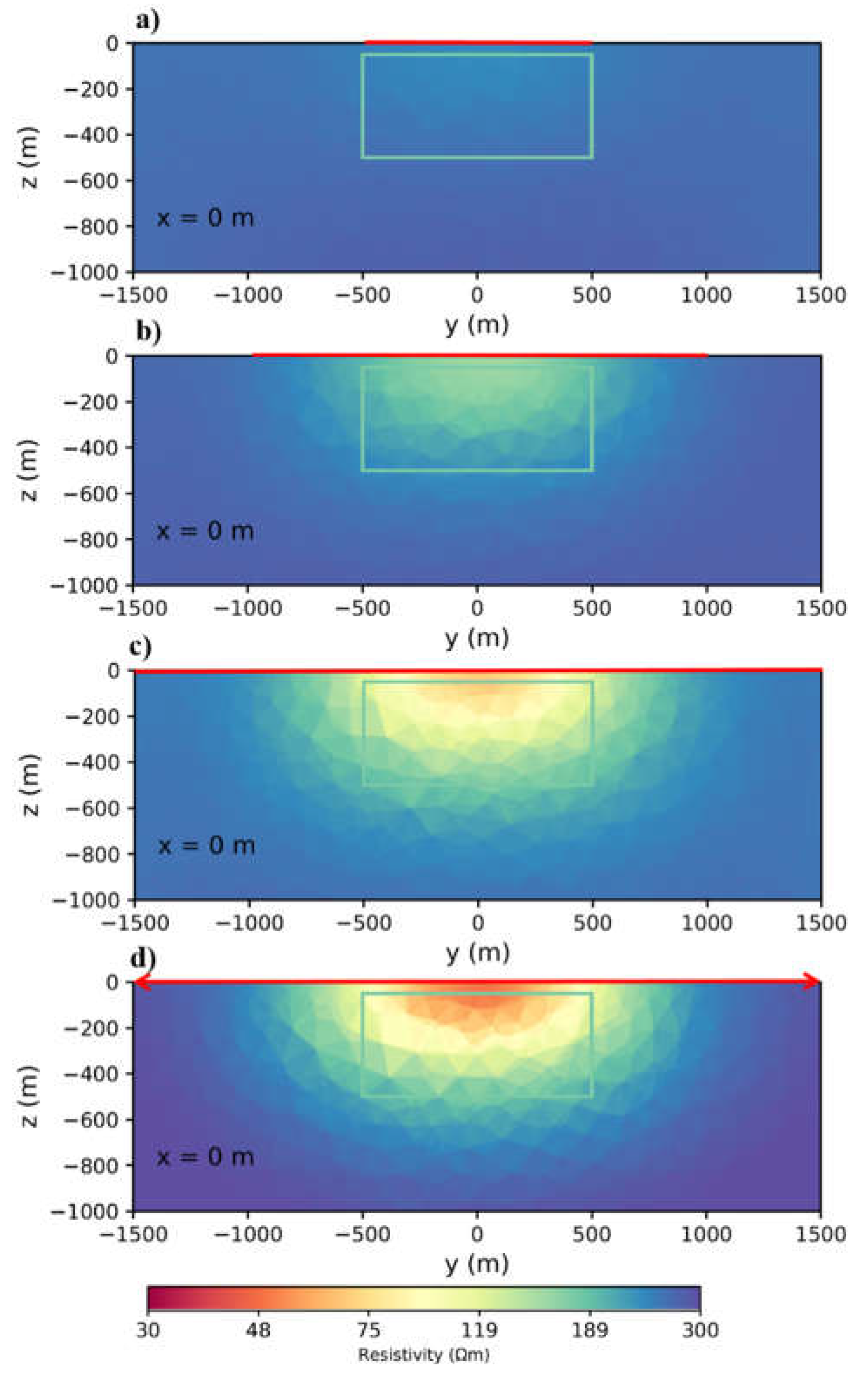
Figure 6.
Inversion results of transmitter at different distance of a. 1 km away from the centre of the conductive body. b. 2 km away from the centre of the conductive body. Transmitter is perpendicular to the general strike of the body.
Figure 6.
Inversion results of transmitter at different distance of a. 1 km away from the centre of the conductive body. b. 2 km away from the centre of the conductive body. Transmitter is perpendicular to the general strike of the body.
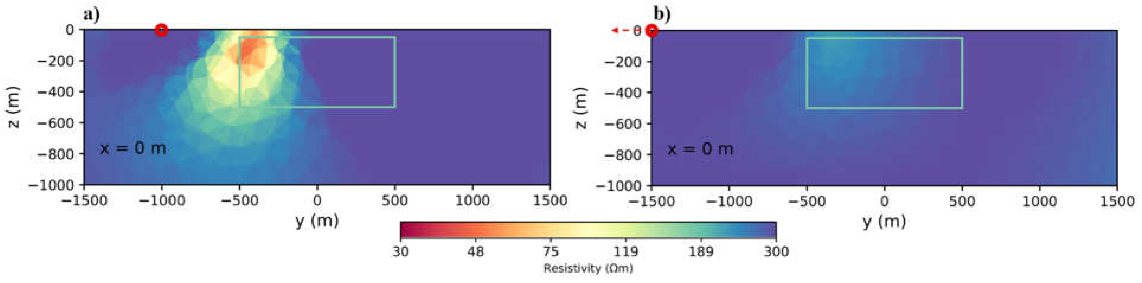
Figure 7.
Inversion result for using single and double transmitters, the first transmitter (Tx1) will be displayed in red and the second transmitter (Tx2) will be displayed in green. Inversion results of a. two conductive bodies and one transmitter. b. Two conductive bodies and two transmitters on both sides.
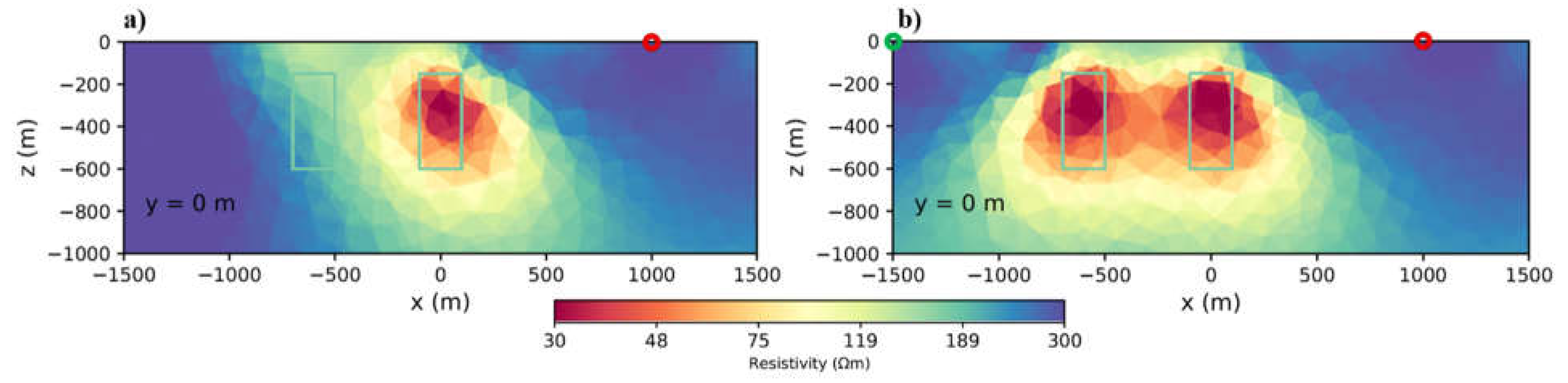
Figure 8.
Inversion results of using two transmitters perpendicular to each other.
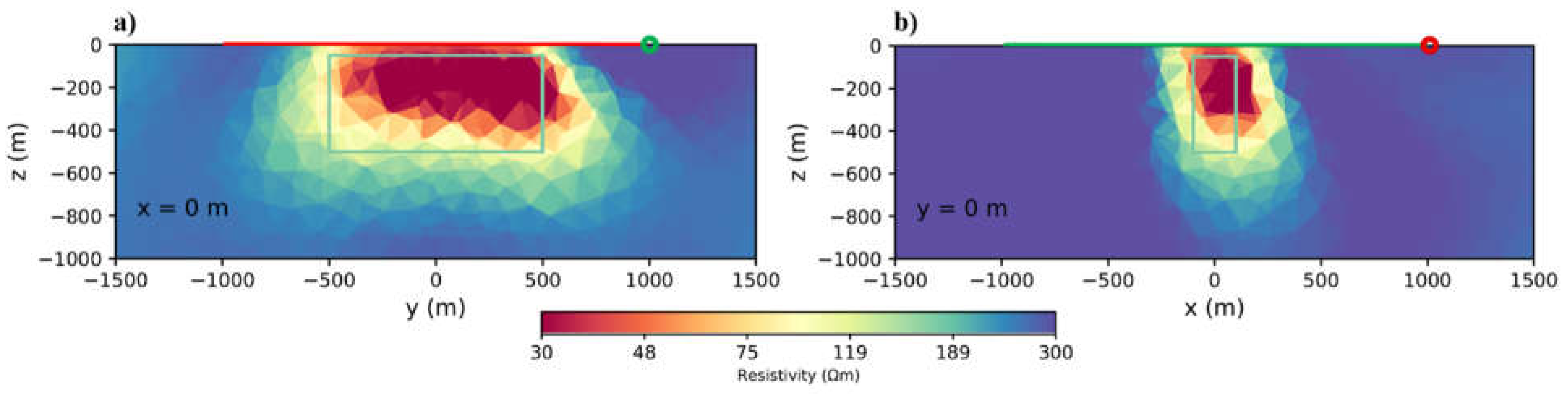
Figure 9.
Inversion results of using two transmitters perpendicular to each other; in this case, the conductive body is a dipping plate. For a better understanding of the plane views please refer to the Appendix Figure A3.
Figure 9.
Inversion results of using two transmitters perpendicular to each other; in this case, the conductive body is a dipping plate. For a better understanding of the plane views please refer to the Appendix Figure A3.
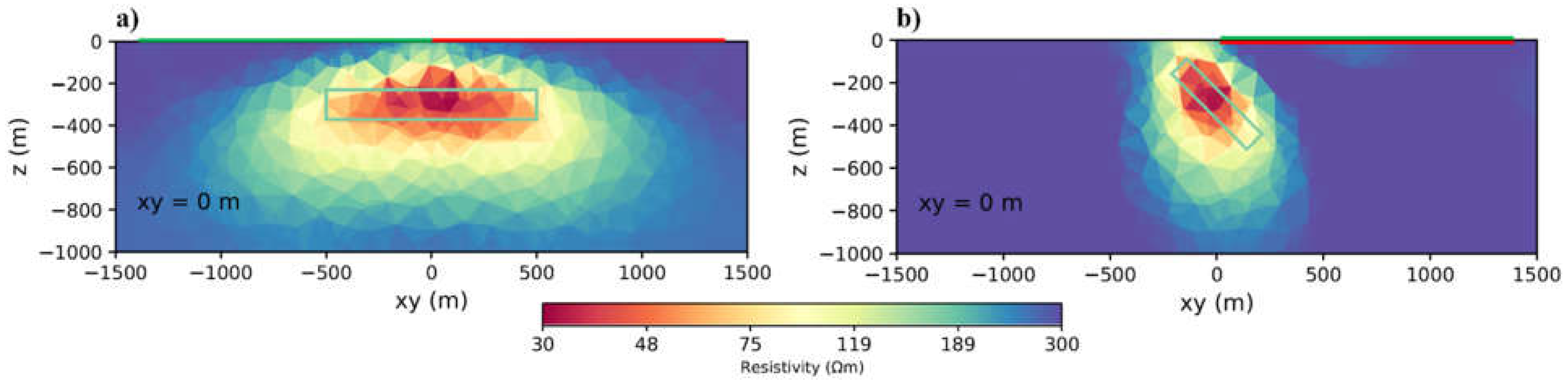
Figure 10.
Inversion results for a body located at different depths: a,b,c: 150 m. d,e,f: 300 m. g,h,i: 500 m from the surface. And for different transmitter distances: a,d,g: 2km, b,e,h: 3km. c,f,i: 4 km.
Figure 10.
Inversion results for a body located at different depths: a,b,c: 150 m. d,e,f: 300 m. g,h,i: 500 m from the surface. And for different transmitter distances: a,d,g: 2km, b,e,h: 3km. c,f,i: 4 km.
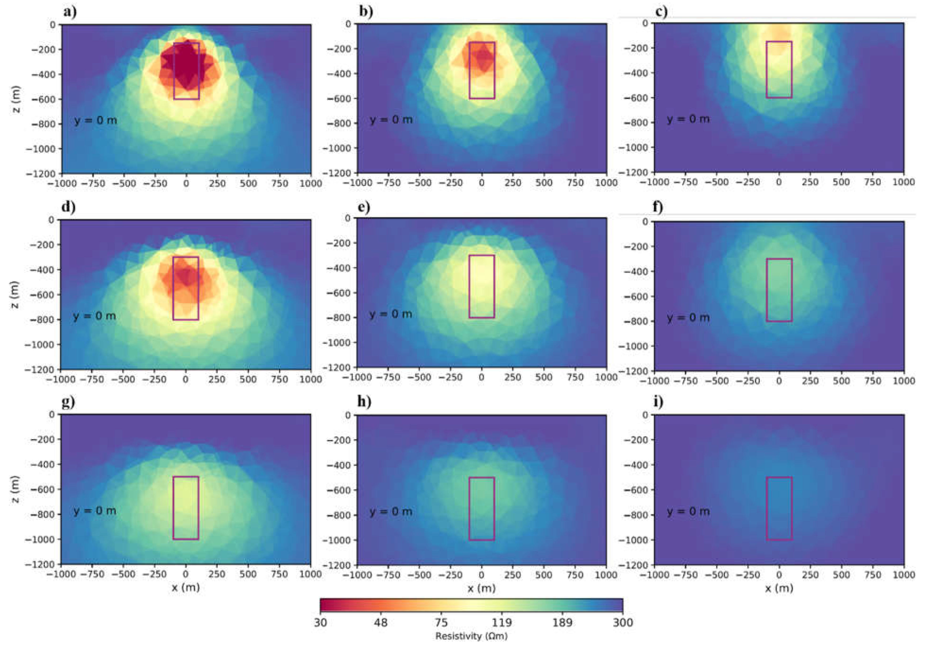
Figure 11.
Inversion results using a body located under the transmitter and different depths below the surface: a, b. 150m . c, d. 300m . e, f. 500m .
Figure 11.
Inversion results using a body located under the transmitter and different depths below the surface: a, b. 150m . c, d. 300m . e, f. 500m .
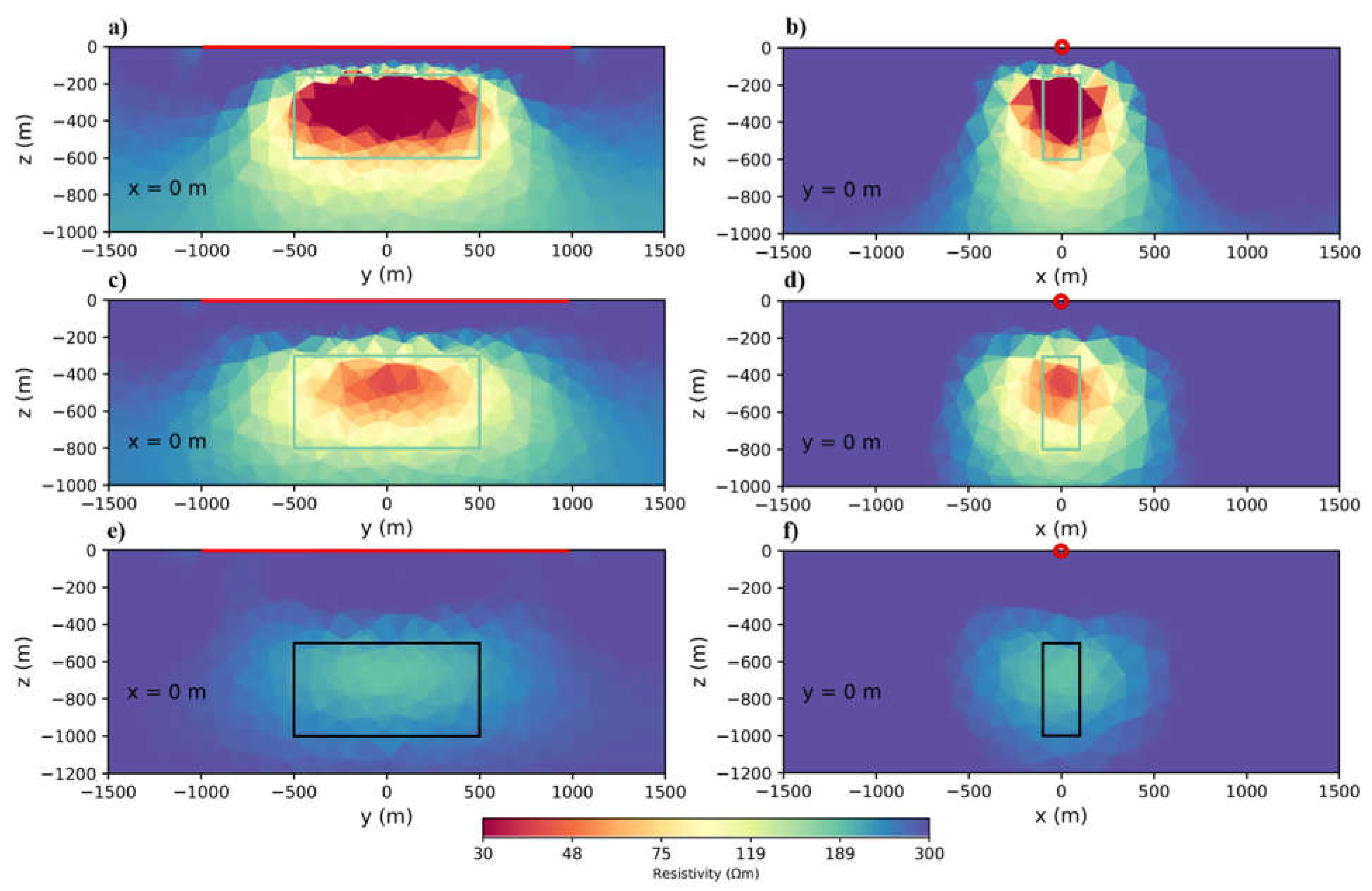
Figure 12.
Inversion results using a body located under two transmitter and different depths of a,b. 150m. c,d. 300m. e,f. 500m. In this case body located exactly under the transmitter Tx1 and 2 km away from transmitter Tx2.
Figure 12.
Inversion results using a body located under two transmitter and different depths of a,b. 150m. c,d. 300m. e,f. 500m. In this case body located exactly under the transmitter Tx1 and 2 km away from transmitter Tx2.
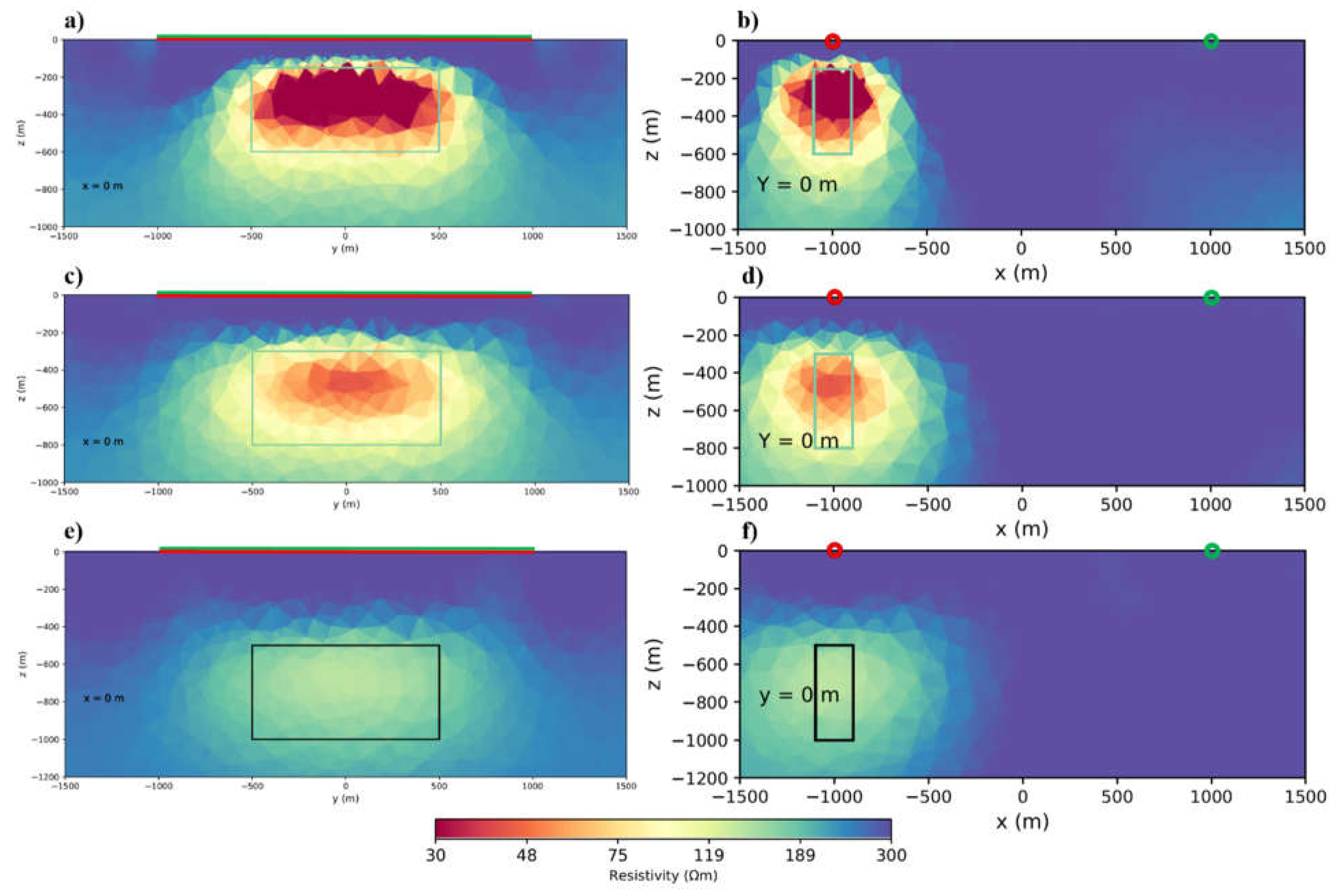
Figure 13.
Recommended optimized survey layout (to be adapted to field conditions). The length of all transmitters and spacing between parallel transmitters is 3 km, using common groundings that reduce logistic effort. Three of the overlapping flight patches are given for example (each covering an area of 24 km2): A over the lower left Tx (dashed blue), B over the lower right Tx (solid blue), and C over the optional Tx (dashed green).
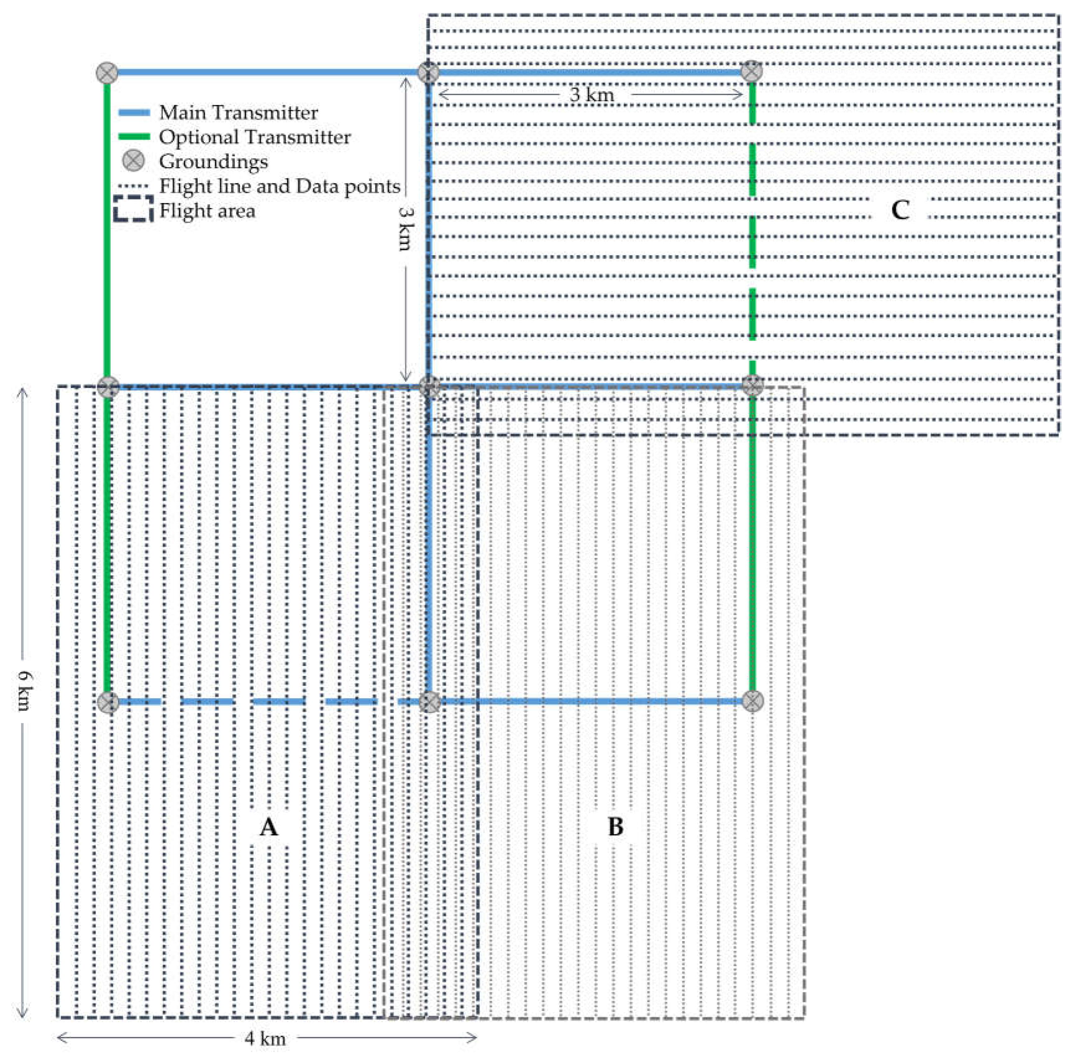

Table 1.
Summary of the data points spacing, number of data points and runtime.
| Grid size (m) | Number of data points | Runtime (Hours) |
|---|---|---|
| 100×100 | 1023 | 19 |
| 200×100 | 528 | 6 |
| 200×200 | 272 | 3 |
Disclaimer/Publisher’s Note: The statements, opinions and data contained in all publications are solely those of the individual author(s) and contributor(s) and not of MDPI and/or the editor(s). MDPI and/or the editor(s) disclaim responsibility for any injury to people or property resulting from any ideas, methods, instructions or products referred to in the content. |
© 2023 by the authors. Licensee MDPI, Basel, Switzerland. This article is an open access article distributed under the terms and conditions of the Creative Commons Attribution (CC BY) license (https://creativecommons.org/licenses/by/4.0/).
Copyright: This open access article is published under a Creative Commons CC BY 4.0 license, which permit the free download, distribution, and reuse, provided that the author and preprint are cited in any reuse.


