
Submitted:
14 April 2023
Posted:
14 April 2023
You are already at the latest version
Abstract
Many problems in the fields of finance and actuarial science can be transformed into the problem of solving backward stochastic differential equations (BSDE) and partial differential equations (PDE) with jumps, which are often difficult to solve in high-dimensional cases. To solve this problem, this paper applies the deep learning algorithm to solve a class of high-dimensional nonlinear partial differential equations with jump terms and their corresponding backward stochastic differential equations (BSDE) with jump terms. Using the nonlinear Feynman-Kac formula, the problem of solving this kind of PDE is transformed into the problem of solving the corresponding backward stochastic differential equations with jump terms, and the numerical solution problem is turned into a stochastic control problem. At the same time, the gradient and jump process of the unknown solution are separately regarded as the strategy function and they are approximated respectively by using two multilayer neural networks as function approximators. Thus, deep learning-based method is used to overcome the “curse of dimensionality” caused by high-dimensional PDE with jump, and the numerical solution is obtained. In addition, this paper proposes a new optimization algorithm based on the existing neural network random optimization algorithm, and compares the results with the traditional optimization algorithm, and achieves good results. Finally, the proposed method is applied to three practical high-dimensional problems: Hamilton-Jacobi-Bellman equation, bond pricing under the jump Vasicek model and high-dimensional option pricing model with default risk. The proposed numerical method has obtained satisfactory accuracy and efficiency. The method has important application value and practical significance in investment decision-making, option pricing, insurance and other fields.
Keywords:
Deep learning
; Backward stochastic differential equation
; Nonlinear Feynman-Kac formula
; High dimensional PDE
; Derivatives pricing
; Neural network
1. Introduction
High-dimensional (dimension ≥ 3) nonlinear partial differential equations (PDEs) are one of the topics that attract much attention and have been widely used in many fields. Many practical problems require the use of high-dimensional PDE, for example: the Schrodinger equation of the quantum many-body problem, whose PDE dimension is about three times that of the electron or quantum (particle) in the system; Black Scholes equation used to price financial derivatives, where the dimension of PDE is the number of relevant financial assets under consideration; Hamilton-Jacobi-Bellman equation in dynamic programming. Although high-dimensional nonlinear partial differential equations have strong practicability, there are few explicit solutions, or the analytical expressions are too complex, so they often need to be solved by some numerical methods. However, in practical applications, high-dimensional nonlinear partial differential equations are usually very difficult to solve, which is still one of the challenging topics in the academic community. The difficulty is that, due to the " curse of dimensionality " [1], the time complexity of traditional numerical solutions will increase exponentially with the increase of dimensions, thus requiring a lot of computing resources. However, because these equations can solve many practical problems, we urgently need to approximate the numerical solution of this high-dimensional nonlinear partial differential equation.
In recent years, deep learning algorithms have gradually emerged and achieved success in many application fields. Therefore, many scientists try to apply deep learning algorithms to solve high-dimensional PDE problems, and have achieved good results. In 2017, E W. Han et al. [2,3] proposed the deep BSDE method and systematically applied the deep learning to general high-dimensional PDE for the first time. After that, Han et al. (2018) [4] further extended the deep BSDE method to the field of random games, and also achieved good results. Beck et al. (2019) [5] extended the method to the case of 2BSDE and the corresponding fully nonlinear PDE. Raissi et al.(2017)[6] use the latest development of probabilistic machine learning to infer the control equation represented by a parametric linear operator, and modifies the prior value of the Gaussian process according to the special form of such operator, which is then used to infer the parameters of the linear equation from the scarce and possibly noisy observations. Sirignano et al. (2018) [7] proposed to use a deep neural network approach to approximate the solution of high-dimensional PDE. In a batch of randomly sampled time and space, the network was trained to meet differential operators, initial conditions and boundary conditions. The above series of achievements show that it is feasible to solve high-dimensional PDE with deep learning-based method.
In this paper, we mainly apply the deep learning algorithm to a special class of high-dimensional nonlinear partial differential equations with jumps, and obtain a numerical solution of the equation. Specifically, through mathematical derivation and equivalent formula expression of high-dimensional PDE and backward stochastic differential equation, the problem of solving partial differential equation is equivalent to the problem of solving BSDE, and then it is transformed into a stochastic control problem. Then, a deep neural network framework is designed to fit the problem. Therefore, this method can be used to solve high-dimensional PDE and corresponding backward stochastic differential equations simultaneously.
The method introduced in this paper to solve a kind of high-dimensional PDE with jump by using deep learning is mainly applied in the financial field, and has important applications in financial derivatives pricing, insurance investment decision-making, small and micro enterprise financing, risk measurement mechanism and other issues.
2. Background Knowledge
2.1. A class of PDE
The Materials and Methods should be described with sufficient details to allow others to replicate and build on the published results. Please note that the publication of your manuscript implicates that you must make all materials, data, computer code, and protocols associated with the publication available to readers. Please disclose at the submission stage any restrictions on the availability of materials or information. New methods and protocols should be described in detail while well-established methods can be briefly described and appropriately cited.
We consider a class of semilinear parabolic PDE with jump term in the following form:
Let , , and and be continuous functions. For all , , function to be solved has a terminal value condition and satisfies:
Where we introduce two operators:
Here is the time variable, is the -dimensional space variable, is the nonlinear part of the equation, represents the gradient of with respect to , represents the Hessian matrix of with respect to . In particular, this equation can be regarded as a special case of partial integro-differential equation. What we are interested in is the solution at , , which is .
2.2. Backward Stochastic Differential Equations with Jumps
Let be a complete probability space, be the d-dimensional standard Brownian motion in this probability space, be the normal filtration generated by in space . , , , are integrable -adapted stochastic processes. For a class of forward backward stochastic differential equations with jump terms, it has the following form:
Where is the compensated Poisson measure, is a centralized Poisson process with the compensator intensity such that , is the Poisson process in the probability space such that .
Under the standard Lipschitz assumptions on the coefficients , , , , , the existence and uniqueness of the solution have been proved. [8]
2.3. The Generalized Nonlinear Feynman-Kac Formula
Under the appropriate regularization assumption, and satisfies equation (1) and linear growth condition , , , the following relationships are established almost everywhere:
2.4. Improvement of Neural Network Parameter Optimization Algorithm
Adam (Adaptive Moment Estimation) algorithm is an algorithm that combines RMSProp algorithm with classical momentum in physics. It dynamically adjusts the learning rate of each parameter by using the first-order moment estimation and second-order moment estimation of gradient. Adam optimizer is one of the most popular classical optimizers in deep learning, and it also shows excellent performance in practice. [11]
Although Adam combines RMSprop with momentum, the adaptive moment estimation with Nesterov acceleration is often better than momentum. Therefore, we consider introducing Nesterov acceleration effect [12] into Adam algorithm, that is, using Nadam (Nesterov-accelerated Adaptive Moment Estimation) optimization algorithm. The calculation formula is as follows:
For parameters of neural network , is the gradient of .Besides, and are the first order moment estimate and the second order moment estimate of the gradient respectively, which can be regarded as the estimation of the expectation and , here and are their attenuation rates respectively. Moreover, and are the correction for and , which can be approximated as an unbiased estimate of the expectation. It can be seen that Nadam has a stronger constraint on the learning rate, and has a more direct impact on the update of the gradient. Therefore, we try to apply the new optimization algorithm to our method and compare the results with the traditional Adam algorithm.
3. Main Theorem
3.1. Basic Ideas
In this paper we propose a deep learning-based PDE numerical solution for nonlinear PDE with jump terms in the form of Equation (2.1). The basic idea of the algorithm are as follows:
By using the generalized nonlinear Feynman-Kac formula, the PDEs to be solved can be equivalently constructed using BSDEs with jumps.
Taking the gradient operator and the jump term of the solution of the function to be solved as policy functions, the problem of solving the numerical solution of BSDEs can be considered as a stochastic control problem, which can be further considered as a reinforcement learning problem.
Two different depth neural networks are used to approximate this pair of high-dimensional strategy functions, and the neural networks are trained by deep learning method to obtain the numerical solution of the original equation.
3.2. Transforming the Nonlinear PDE Numerical Solution Problem into a Stochastic Control Problem
It is well known that PDE and BSDE can be linked by the generalized nonlinear Feynman-Kac formula under appropriate assumptions. Thus, the solution of the above equation is equivalent to the viscous solution of the semilinear parabolic PDE partial differential equation with jump term in (2.1). [13,14] Because the numerical solution of the traditional partial differential equation does not perform well in high dimensions, we can estimate the solution of equation (2.1) by estimating the solution of equation (2.4).
For the stochastic control problem related to equation (2.4), under the appropriate regularity assumption, for the nonlinear function , it holds that a group of solution functions composed of , and is the unique global minimum of the following functions :
We regard and as the policy function of deep learning problem, and use DNN to approximate and . In this way, the stochastic process corresponds to the solution function of the stochastic control problem and can be solved by using the strategy functions and , and thus we can transform the nonlinear partial differential equation into a stochastic control problem.
3.3. Forward Discretization of the Backward Stochastic Differential Equations with Jumps
For the following BSDE:
We will discretize it in the time dimension and divide the time interval into N partitions, so that and , assuming , we use Euler scheme for discretization:
Where , , .
In this way we can start from the initial value of (3.2) and finally obtain the approximation of the Euler format of (3.2) at N partitions.
3.4. General Framework for Neural Networks
Two feedforward neural networks are established at each time step in (3.3) and (3.4). One is to approximate the gradient of the unknown solution, which means to approximate the function , and this neural network is recorded as , such that represents all parameters of this neural network and indicates that this neural network is used to approximate at time . Another is to approximate the jump process of the unknown solution, which means to approximate the function and this neural network is recorded as , such that represents all parameters of this neural network, and indicates that this network is used to approximate at time . For the convenience of expression, we can suppose ,, . As shown in Figure 1, all sub neural networks are stacked together to form a complete neural network.
in the initial layer is a random variable. , and in the initial layer is unknown, and we treat it as parameters of the neural network. And , and corresponds to the value of the BSDE with jumps as follows:
And
In this neural network, the of the current layer is related to the of the previous layer, and at the same time the of the current layer is related to the , , and of the previous layer. However, there are no and in the current layer. Therefore, as shown in the Figure 1, our solution is to start from the of the current layer to build two sub neural networks to represent these two values. In addition, the construction of the final loss function can be obtained from a given terminal value condition , that is, in the neural network, which also corresponds to in the nonlinear Feynman-Kac formula.
Specifically, for , we can set , as parameters to obtain the appropriate Euler approximation of the process forward:
For all appropriate , we have . For all appropriate , we have . Then we can get a suitable approximation of :
The mean square error between the final output of neural network and the true value at the terminal time is selected as the loss function:
is the set of all training parameters of the above system, such that . This loss function is used since . And the expectation in the loss function in (3.10) is the expectation for all sample paths, but due to the infinite number of sample paths, it is not possible to traverse the entire training set. Therefore, we adopt an optimization method based on stochastic gradient descent. In each iteration of gradient descent, only a portion of samples are selected to estimate the loss function, thereby obtaining the gradient of the loss function over all parameters, and obtaining a one-step neural network parameter update.
Like this, the back propagation of this neural network uses optimizer to update the parameters layer by layer. When DNN is trained, is fixed as the parameter value. Take this parameter value out and it is the required value.
3.5. Details of the Algorithms
The detailed steps of our proposed algorithm based on deep learning to numerically solve the BSDE with jumps is presented as follows.
According to our algorithm, which uses a deep learning-based neural network solver, the BSDE with jumps in the form of equation (2.4) can be numerically solved in the following ways:
- Simulate sample paths using standard Monte Carlo methods
- Use a deep neural network (DNN) to approximate and, and then plug them into the BSDE with jumps to perform a forward iterative operation in time
For simplicity, here we use the one-dimensional case as an example, and the high-dimensional case is similar. We divide the time interval into N partitions, so that and , assuming , and . The detailed steps are as follows:
- (1)
- N Monte Carlo paths of the diffusion process are sampled by Euler scheme:
This step is the same as the standard Monte Carlo method. Other discretization schemes can also be used, such as logarithmic Euler discretization or Milstein discretization.
- (2)
- At , the initial value , and is randomly selected as parts of the neural network parameters, and , and are all constant random numbers selected from an empirical range.
- (3)
- At each time step , given , and are approximated using deep neural networks, respectively. Note that every time , two sub neural networks are used for all Monte Carlo paths. In our one-dimensional case, as described in Section 3.4, we introduce two sub deep neural networks: , such that and , such that . And , , .
- (4)
- For , we have
According to this formula, we can directly calculate the at the next time step. This process does not require any parameters to be optimized. In this way, the BSDE with jumps propagates forward in time direction from to . Along each Monte Carlo path, as the BSDE with jumps propagating forward in time from 0 to T, is estimated as , where is all the hyper-parameters for the N-1 layers neural networks.
- (5)
- Calculate the following loss function:
Where g is the terminal function.
- (6)
- Use stochastic optimization algorithms to minimize the loss function:
The estimated value is the desired initial value at time t=0.
4. Numerical Results
In this section, we will use the depth neural network to code the theoretical framework of the proposed algorithm. In this paper, three classical high-dimensional PDEs with important applications in finance-related fields are selected for numerical simulation, they are: financial derivative pricing under jump-diffusion model, Bond pricing under Vasicek model with jump, Hamilton-Jacobi-Bellman equation.
The numerical experiments in this paper uses a 64-bit Windows 10 operating system, based on the PyTorch deep learning framework in Python. All examples in this section are calculated based on 1000 sample paths, each chosen for a time partition of N = 100. We ran each example 10 times independently to calculate the average result. All neural network parameters will be initialized by uniform distribution. Each sub neural network of each time node contains 4 layers: one d-dimensional input layer, two (d+10)-dimensional hidden layers, one d-dimensional output layer. We use the rectifier function (ReLU) as the activation function. Batch Normalization (BN) techniques are used after each linear transformation and before activation.
4.1. Pricing of Financial Derivatives under Jump Diffusion Model
In this section, we will apply the proposed method to the pricing of derivatives related to a 100-dimensional jump diffusion model. In this model, the stock price satisfies the following jump diffusion model [15]:
| if an asset price does not jump | |
| if an asset price jumps |
Where is the constant discount rate, is the average number of jumps per unit time of the stock price, is the constant volatility. represents the jump magnitude. Assuming that the jump amplitude is fixed and V is constant, we can let and . This equation can be written as .
It is known that the European call option with the stock as the underlying asset satisfies the following partial differential equation:
For all , , , . Suppose , , , , , , , , , , here , , are randomly selected in , .
After calculation, Table 1 and Table 2 show the important numerical results of solving the related derivative pricing problem of the 100-dimensional jump diffusion model with Adam and NAdam optimizers respectively, including that with the change of iteration steps, mean and standard deviation of loss function , mean and standard deviation of loss function, and running time. Only the numerical results of iteration steps are selected as typical examples for display.
It can be seen from Table 1 and Table 2 that when the iteration steps are the same, the calculation time required for using the two optimizers is not very different. As the iteration progresses, the loss function value of the Nadam optimizer is smaller than that of the Adam optimizer at the same iteration steps, and the final loss function value is also smaller.
Figure 2 and Figure 3 show the changes of the initial value estimate and loss function with the number of iteration steps when Adam and NAdam optimizers are used for solving. It can be seen that the initial value estimates and loss functions of the numerical solutions of the two methods converge rapidly. However, the convergence speed of the latter is obviously faster than that of the former, whether it is the initial value estimate or the loss function. Among them, the former tends to converge after about 1500 iterations, while the latter tends to converge after about 700 iterations. When the iteration is 4000 times, the numerical solution obtained by Adam algorithm is 0.32143775, while the numerical solution obtained by NAdam algorithm is 0.32273737, which is similar.
4.2. Bond Pricing under the Jumping Vasicek Model
In this section, we use the proposed method to solve the pricing problem of a class of bonds with interest rates subject to the Vasicek model with jumps. [16,17] In this model, short-term interest rate obeys the following stochastic differential equations:
i.e., each part of follows:
For all , , , . Suppose , , , , , , , , , are randomly selected in, , . Then, for the zero-coupon bond price paying 1 at maturity T under the above jump Vasicek model, it satisfies that for all , , and the following partial differential equation holds:
After calculation, Table 3 and Table 4 show the important numerical results of solving a class of bond pricing problems with interest rates subject to the Vasicek model with jumps using Adam and NAdam optimizers respectively, including that with the change of iteration steps, mean and standard deviation of loss function , mean and standard deviation of loss function, and running time. Only the numerical results of iteration steps are selected as typical examples for display.
It can be seen from Table 3 and Table 4 that with the iteration, the loss function value of the NAdam optimizer is smaller than that of the Adam optimizer at the same iteration steps, and the final loss function value is smaller, but the cost is that the operation time becomes longer.
Figure 4 and Figure 5 show the changes of the initial value estimate and loss function with the number of iteration steps when Adam and NAdam optimizers are used for solving. It can be seen that the initial value estimates and loss functions of the numerical solutions of the two methods converge rapidly. However, the convergence speed of the latter is obviously faster and more stable than the former, whether it is the initial value estimate or the loss function. When the iteration is 4000 times, the numerical solution obtained by Adam algorithm is 0.25530547, while the numerical solution obtained by NAdam algorithm is 0.27403888. The difference is not significant.
4.3. Hamilton-Jacobi-Bellman (HJB) Equation
In fields such as finance, investment, and risk management, optimization and control problems are often involved, and these problems are often represented by stochastic optimal control models. One way to solve this kind of control problem is to obtain and solve the Hamilton-Jacobi-Bellman equation (HJB equation for short) of the corresponding control problem according to the principle of dynamic programming. In this section, we use the proposed method to solve a class of 100-dimensional HJB equations [9]:
For all , , , . Suppose , , , , , , , , where,are randomly selected in , , , it satisfies that for all , , and the following partial differential equation holds:
After calculation, the important numerical results of solving a class of HJB equations with Adam and NADam optimizers are shown in Table 5 and Table 6 respectively, including that with the change of iteration steps, mean and standard deviation of loss function , mean and standard deviation of loss function, and running time. Only the numerical results of iteration steps are selected as typical examples for display.
It can be seen from Table 5 and Table 6 that with the iteration, the loss function value of the NAdam optimizer is smaller than that of the Adam optimizer at the same iteration steps, and the final loss function value is smaller, but the operation time is longer.
Figure 6 and Figure 7 show the changes of the initial value estimate and loss function with the number of iteration steps when Adam and NAdam optimizers are used for solving. It can be seen that the convergence speed of the latter is obviously faster than that of the former, whether it is the initial value estimate or the loss function. Among them, the former tends to converge after about 7000 iterations, while the latter tends to converge after about 5500 iterations. After 8000 iterations, the numerical solution obtained by Adam algorithm is 2.73136686, while the numerical solution obtained by NAdam algorithm is 2.6456454, with little difference between the two.
5. Conclusions
In this paper, we propose an algorithm that can be used to solve a class of partial differential equations with jump terms and their corresponding backward stochastic differential equations. Through the nonlinear Feynman-Kac formula, the above-mentioned high-dimensional nonlinear PDE with jumps and its corresponding BSDE can be expressed equivalently, and the numerical solution problem can be regarded as a stochastic control problem. Next, we treat the gradient and jump process of the unknown solution separately as policy functions, and use two neural networks at each time division to approximate the gradient and jump process of the unknown solution respectively. In this way, we can use deep learning to solve the " curse of dimensionality " caused by high-dimensional PDE with jumps and obtain numerical solutions.
Among them, jump process can depict the sudden impact of the outside world in its process, so that it can accurately depict a class of uncertain things, and this situation is most common in financial markets. In this way, we extend the numerical solution problem of high-dimensional PDE to the case of jump diffusion. Furthermore, we can use this algorithm to solve a series of problems in finance, insurance, actuarial modeling and other fields, such as the pricing problem of some special path dependent financial derivatives, and the bond pricing problem under the jump diffusion model of interest rates.
In addition, we attempt to replace the traditional Adam algorithm with the new stochastic optimization approximation algorithm and apply it to our algorithm. Next, focusing on the financial field, we applied our algorithm to solve three common high-dimensional problems in finance-related fields and then compared the results. We concluded that our algorithm performs well in numerical simulation. It is also concluded that after applying the new optimizer to the deep learning algorithm, the convergence speed of the model is mostly faster, and the generalization ability is significantly improved, at the cost of the operation time may be longer.
Funding
This research received no external funding.
Conflicts of Interest
The authors declare no conflict of interest.
References
- Kang, W. , Wilcox L. C. Mitigating the curse of dimensionality: sparse grid characteristics method for optimal feedback control and HJB equations. Computational Optimization and Applications 2017, 68, 289–315. [Google Scholar] [CrossRef]
- E. W., Han J., Jentzen A. Deep learning-based numerical methods for high-dimensional parabolic partial differential equations and Backward Stochastic Differential Equations. Communications in Mathematics and Statistics 2017, 5, 349–380. [Google Scholar] [CrossRef]
- Han, J. , Jentzen A., E W. Solving high-dimensional partial differential equations using deep learning. Proceedings of the National Academy of Sciences of the United States of America 2018, 115, 8505–8510. [Google Scholar] [CrossRef] [PubMed]
- Han, J. , Hu R. Deep fictitious play for finding Markovian Nash equilibrium in multi-agent games. Proceedings of The First Mathematical and Scientific Machine Learning Conference 2020, 107, 221–245. [Google Scholar]
- Beck, C. , E W., Jentzen A. Machine learning approximation algorithms for high-dimensional fully nonlinear partial differential equations and second-order backward stochastic differential equations. Journal of Nonlinear Science 2019, 29, 1563–1619. [Google Scholar] [CrossRef]
- Raissi M, Perdikaris P. , Karniadakis G. E. Machine learning of linear differential equations using Gaussian processes. Journal of Computational Physics 2017, 348, 683–693. [Google Scholar] [CrossRef]
- Sirignano, J. , Spiliopoulos K. DGM: A deep learning algorithm for solving partial differential equations. Journal of Computational Physics 2018, 375, 1339–1364. [Google Scholar] [CrossRef]
- S. Tang, X. Li, Necessary conditions for optimal control of stochastic systems with random jumps. SIAM Journal on Control Optimization 1994, 32, 1447–1475.
- Rong, S. , Theory of stochastic differential equations with jumps and applications[M]. London: Springer, 2005. 205-290.
- Łukasz Delong, Backward stochastic differential equations with jumps and their actuarial and financial applications [M]. London: Springer, 2013. 85-88.
- Henry-Labordere P, Oudjane N, Tan X, Touai N, Warin X, et al. Branching diffusion representation of semilinear PDEs and Monte Carlo approximation. Annales de 1’Institut Henri Poincar"e, Probabilit"es et Statistiques 2019, 55, 184–210. [Google Scholar]
- Ilya Sutskever, James Martens, George Dahl, and Geoffrey Hinton, On the importance of initialization and momentum in deep learning[C]. Proceedings of the 30th International Conference on Machine Learning ICML 2013. pages 1139–1147, 2013.
- G. Barles, R. Buckdahn, E. Pardoux, Backward stochastic differential equations and integral-partial differential equations. Stochastics Reports 1997, 60, 57–83. [Google Scholar] [CrossRef]
- R. Buckdahn, E. Pardoux, BSDE’s with jumps and associated integro-partial differential equations[M]. Preprint.
- Merton R, C. , Option Pricing when Underlying Stock Returns are Discontinuous. Journal of Financial Economics 1976, 3, 125–144. [Google Scholar] [CrossRef]
- Li, S. , Zhao X., Yin C., et al. Stochastic interest model driven by compound Poisson process and Brownian motion with applications in life contingencies. Quantitative Finance and Economic 2018, 2, 731–745. [Google Scholar] [CrossRef]
- Jiang, Y. , Li J., Convergence of the Deep BSDE method for FBSDEs with non-Lipschitz coefficients. Probability, Uncertainty and Quantitative Risk 2021, 6, 391–408. [Google Scholar] [CrossRef]
Figure 1.
Deep neural network framework.
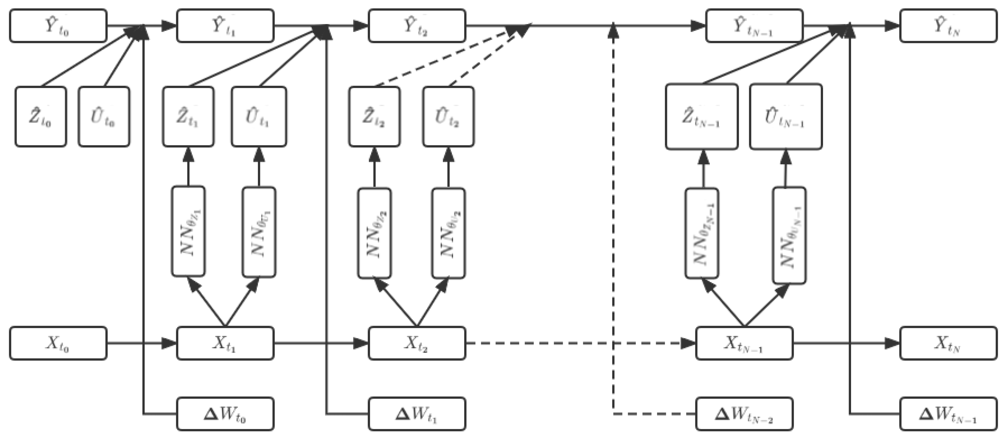
Figure 2.
Changes of initial value estimation and loss function with iteration steps under Adam optimizer.
Figure 2.
Changes of initial value estimation and loss function with iteration steps under Adam optimizer.
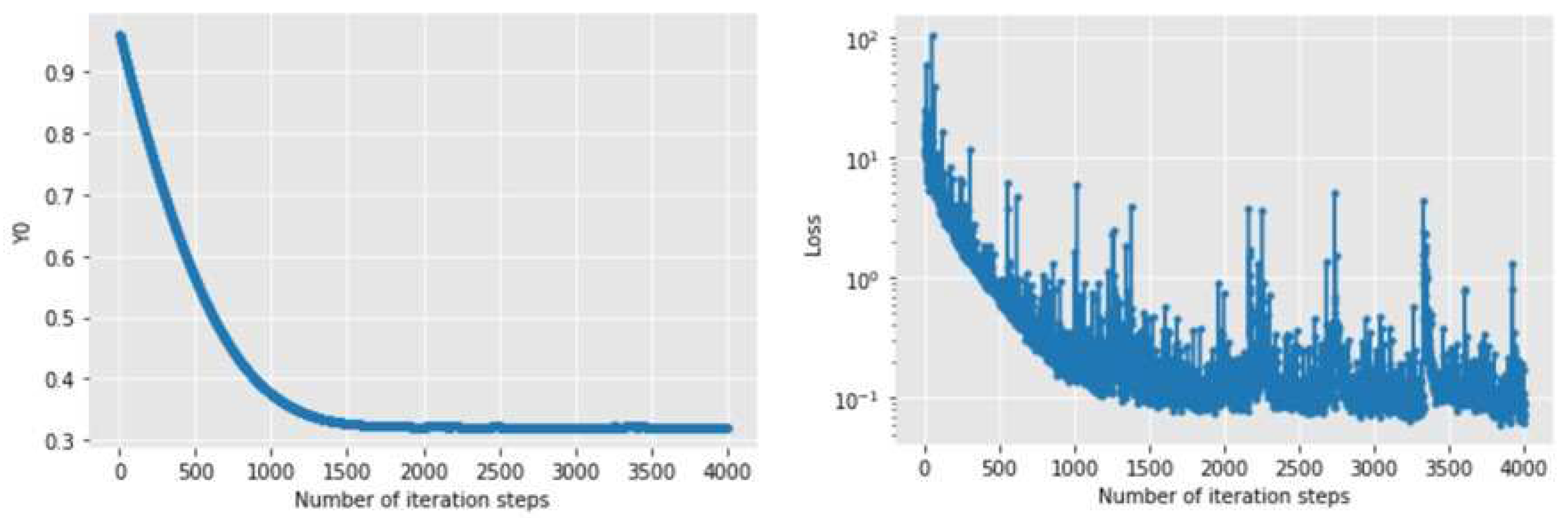
Figure 3.
Changes of initial value estimation and loss function with iteration steps under NAdam optimizer.
Figure 3.
Changes of initial value estimation and loss function with iteration steps under NAdam optimizer.
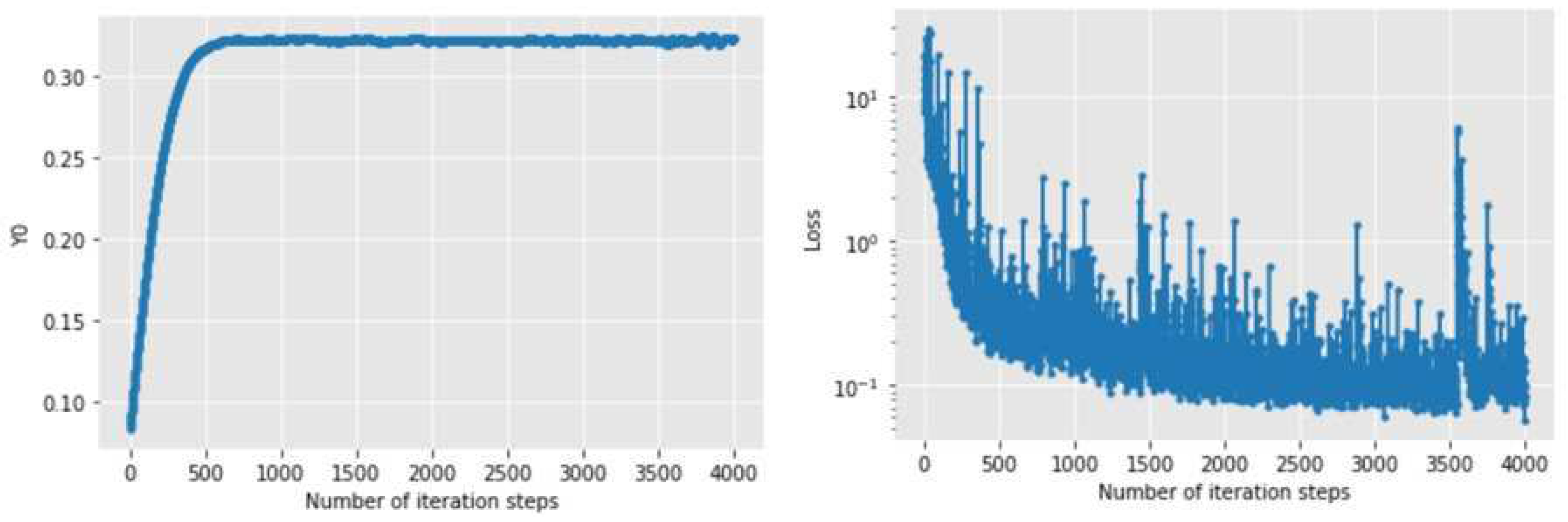
Figure 4.
Changes of initial value estimation and loss function with iteration steps under Adam optimizer.
Figure 4.
Changes of initial value estimation and loss function with iteration steps under Adam optimizer.
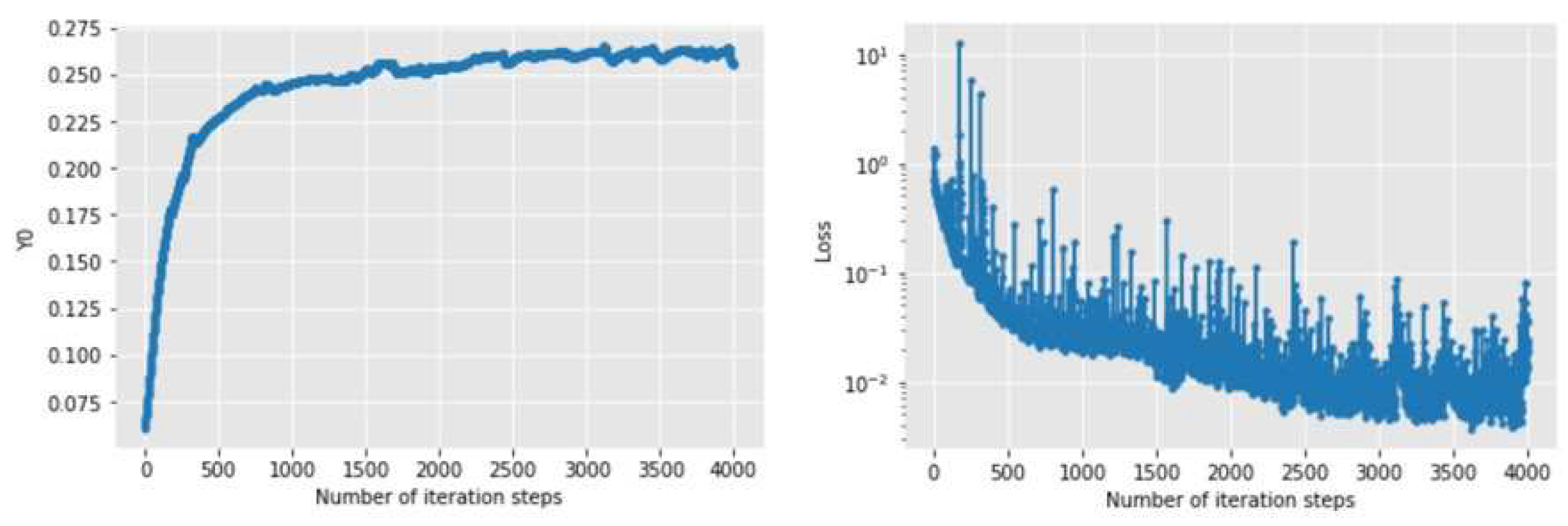
Figure 5.
Changes of initial value estimation and loss function with iteration steps under NAdam optimizer.
Figure 5.
Changes of initial value estimation and loss function with iteration steps under NAdam optimizer.
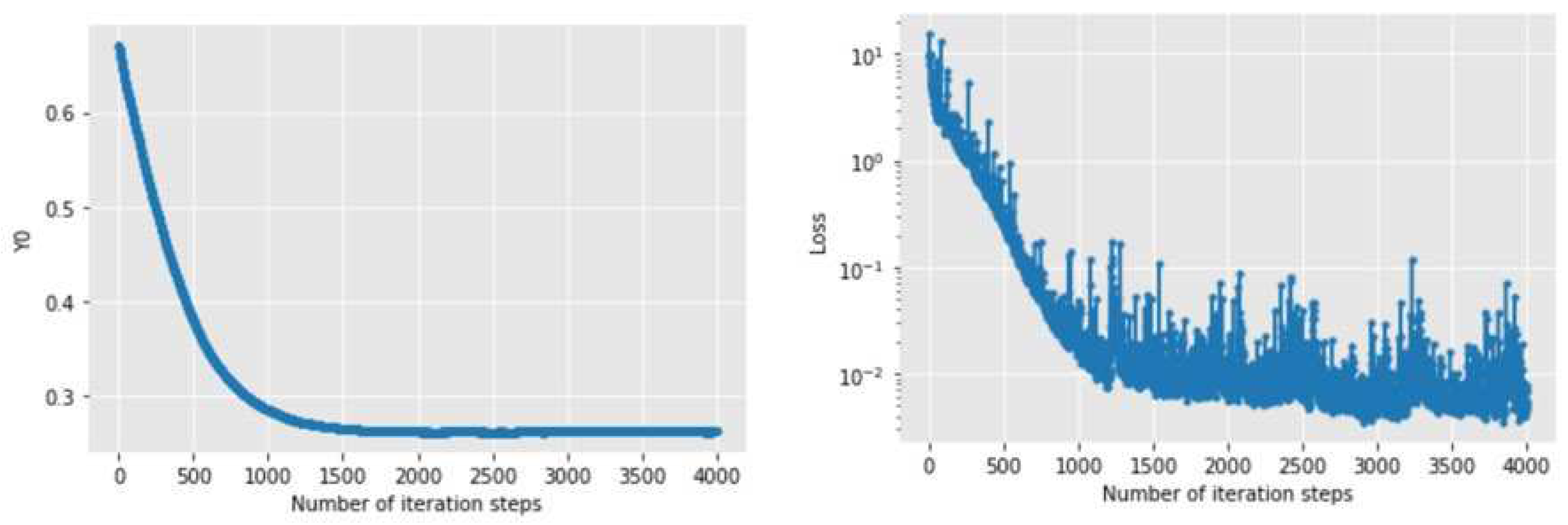
Figure 6.
Changes of initial value estimation and loss function with iteration steps under Adam optimizer.
Figure 6.
Changes of initial value estimation and loss function with iteration steps under Adam optimizer.
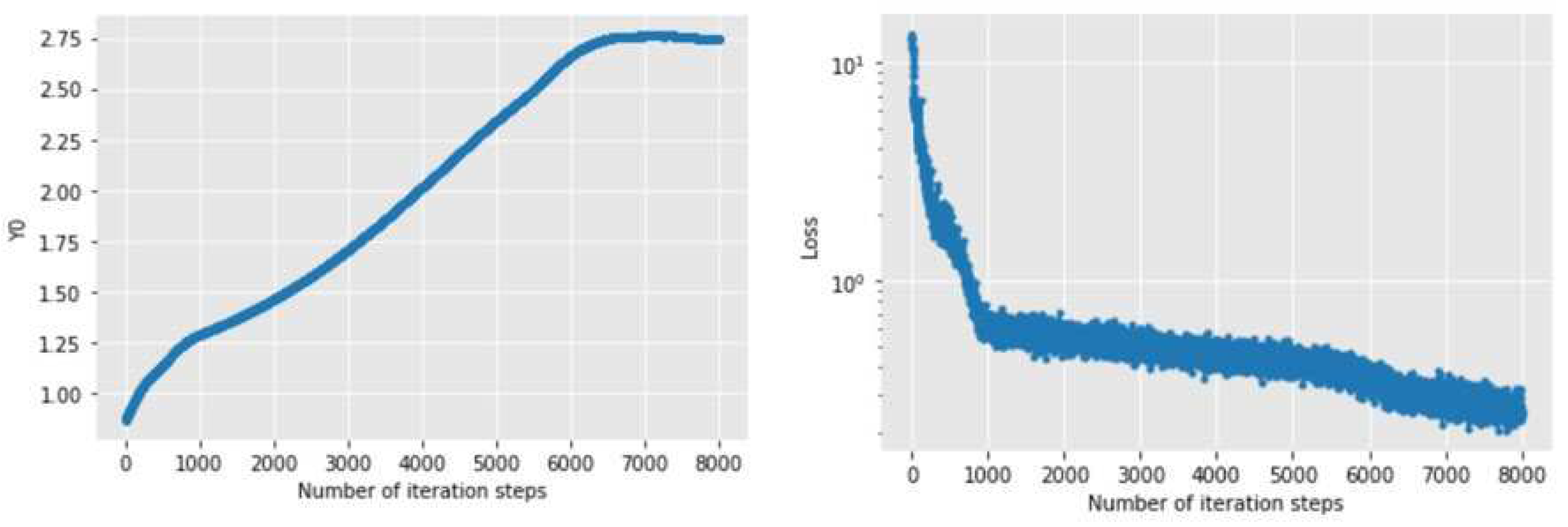
Figure 7.
Changes of initial value estimation and loss function with iteration steps under NAdam optimizer.
Figure 7.
Changes of initial value estimation and loss function with iteration steps under NAdam optimizer.
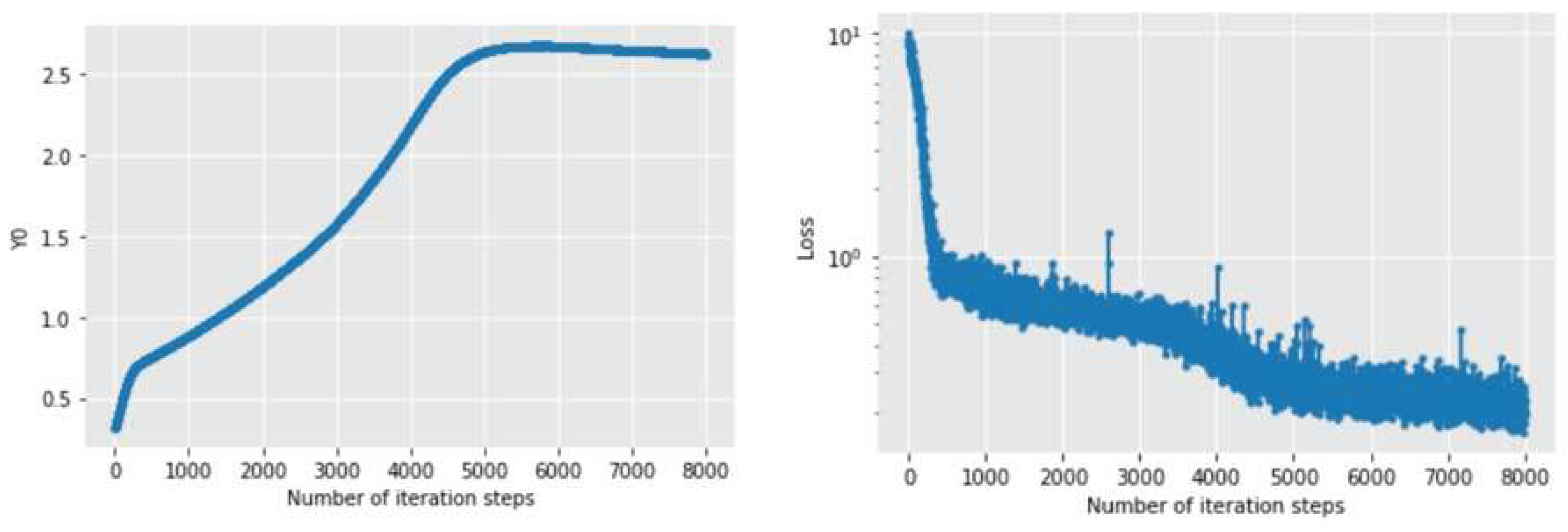

Table 1.
Numerical results with Adam optimizer.
| Number of iteration steps m | Mean of the loss function | Standard deviation of the loss function | Runtime in second | ||
|---|---|---|---|---|---|
| 1000 | 0.5989 | 0.1719 | 1.2743 | 7.7509 | 474 |
| 2000 | 0.4664 | 0.1235 | 1.2532 | 4.3095 | 891 |
| 3000 | 0.4183 | 0.1623 | 1.0894 | 3.7375 | 1271 |
| 4000 | 0.3940 | 0.1465 | 0.6269 | 2.4771 | 1676 |
Table 2.
Numerical results with NAdam optimizer.
| Number of iteration steps m | Mean of the loss function | Standard deviation of the loss function | Runtime in second | ||
|---|---|---|---|---|---|
| 1000 | 0.2821 | 0.0625 | 1.1528 | 2.7450 | 549 |
| 2000 | 0.3019 | 0.0484 | 0.6747 | 2.0031 | 828 |
| 3000 | 0.3084 | 0.0406 | 0.4911 | 1.6566 | 1206 |
| 4000 | 0.3117 | 0.0356 | 0.4134 | 1.4535 | 1651 |
Table 3.
Numerical results with Adam optimizer.
| Number of iteration steps m | Mean of the loss function | Standard deviation of the loss function | Runtime in second | ||
|---|---|---|---|---|---|
| 1000 | 0.2096 | 0.0435 | 0.1405 | 0.4825 | 538 |
| 2000 | 0.2300 | 0.0370 | 0.0820 | 0.3464 | 924 |
| 3000 | 0.2396 | 0.0331 | 0.0585 | 0.2849 | 1296 |
| 4000 | 0.2450 | 0.0302 | 0.0463 | 0.2476 | 1779 |
Table 4.
Numerical results with NAdam optimizer.
| Number of iteration steps m | Mean of the loss function | Standard deviation of the loss function | Runtime in second | ||
|---|---|---|---|---|---|
| 1000 | 0.2828 | 0.0293 | 0.0323 | 0.1310 | 652 |
| 2000 | 0.2772 | 0.0215 | 0.0224 | 0.1033 | 1326 |
| 3000 | 0.2757 | 0.0177 | 0.0172 | 0.0855 | 1957 |
| 4000 | 0.2750 | 0.0154 | 0.0150 | 0.0753 | 2581 |
Table 5.
Numerical results with Adam optimizer.
| Number of iteration steps m | Mean of the loss function | Standard deviation of the loss function | Runtime in second | ||
|---|---|---|---|---|---|
| 2000 | 1.2504 | 0.1521 | 1.3142 | 1.4709 | 857 |
| 4000 | 1.4850 | 0.2820 | 0.9090 | 1.1166 | 1770 |
| 6000 | 1.7704 | 0.4768 | 0.7447 | 0.9412 | 2906 |
| 8000 | 2.0139 | 0.5904 | 0.6314 | 0.8386 | 3864 |
Table 6.
Numerical results with NAdam optimizer.
| Number of iteration steps m | Mean of the loss function | Standard deviation of the loss function | Runtime in second | ||
|---|---|---|---|---|---|
| 2000 | 0.8762 | 0.1941 | 1.2294 | 1.5767 | 1649 |
| 4000 | 1.2456 | 0.4419 | 0.8682 | 1.1733 | 3104 |
| 6000 | 1.6858 | 0.7241 | 0.6715 | 0.9980 | 4527 |
| 8000 | 1.9266 | 0.7531 | 0.5606 | 0.8855 | 5948 |
Disclaimer/Publisher’s Note: The statements, opinions and data contained in all publications are solely those of the individual author(s) and contributor(s) and not of MDPI and/or the editor(s). MDPI and/or the editor(s) disclaim responsibility for any injury to people or property resulting from any ideas, methods, instructions or products referred to in the content. |
© 2023 by the authors. Licensee MDPI, Basel, Switzerland. This article is an open access article distributed under the terms and conditions of the Creative Commons Attribution (CC BY) license (http://creativecommons.org/licenses/by/4.0/).
Copyright: This open access article is published under a Creative Commons CC BY 4.0 license, which permit the free download, distribution, and reuse, provided that the author and preprint are cited in any reuse.


