
Submitted:
19 April 2023
Posted:
20 April 2023
Read the latest preprint version here
Abstract
We present a new model formulation for a class of capacitated lot-sizing problem considering setup costs, product returns, and remanufacturing (CLSP-RM). We investigate a broad class of instances that fall into two groups, in the first group we can reformulate the problem with a relaxation and test whether the original problem is solvable. The relaxation gives near optimal solutions and the solution of this class does not give any difficulty to known solvers such as Cplex, Gurobi or Xpress. The second group of instances are of category NP and will be solved with a simple period-by-period simulation
Keywords:
Simulation based optimization
; capacitated lot-sizing problem
; heuristics
; remanufacturing
1. Introduction
The production planning with consideration of recycling options has received increasing attention in the last few years [1]. The literature describes two different categories of recycling production planning problems. In the first category (Cat. 1), the given external demand of the products has to be satisfied by remanufactured or newly produced goods Figure 1. Only two types of inventories are regulated: the inventory of new products and the inventory of remanufactured products, and this is the category that has been thoroughly investigated by numerous authors. It is assumed that new and remanufactured products are identical, and hence, both are regarded as serviceables, i.e., entities that can be used to satisfy demands. In the second category (Cat. 2) the additional feature of this problem is that in each period a deterministic amount of returned items enters the system. These returns can be remanufactured and used to satisfy the demand for remanufactured products in addition to the regular production of new items. Thus, there are three types of inventory: new product inventory, remanufactured product inventory and returned product inventory (Figure 1). This situation is typical in paper manufacturing. Demand for recovered paper has increased enormously worldwide, making separate collection more attractive again. Peter Probst, CEO of LEIPA Group, Germany (Viadrina University, 05.2019) explains the advantage: "paper recycling proves to be economically and ecologically efficient, because the production of recycled paper requires considerably less water and considerably less energy than the production of virgin fiber papers. In addition, the transport distances are generally shorter as well. Recycled paper comes from Germany, while the fresh fibers and fresh fiber papers are also imported to Germany in larger proportions". Paper production is also energy intensive. It takes as much energy to produce one ton of paper from fresh wood fibers as it does to produce one ton of steel ([2]).
2. Literature Review
Publications regarding Category 1: [3] analyzes several CLSP-RM formulations with the column generation method, where he uses the idea of Garfinkel and Nemhauser (1969), namely the Set Partitioning Problem (SPP). [4] compared MIP approaches to the economic lot-sizing with remanufacturing (ELSR) and proposes a shortest path formulation. [5] studied another multi-item variant of the problem and propose a variable neighborhood search heuristic. The polynomial-time heuristics of [6] also belongs to this category, where there is also an excellent compilation of the methods developed by [7,8,9,10,11].
Publications regarding category 2: The only publication known to us is that of [12] where he presents a Lagrange relaxation to solve the problem. Based on Zhang’s model we formulate the same problem but taking more general capacity constraints and doing more extensive numerical experiments.
The capacitated lot sizing problem model is NP-hard. The proof of this statement is to be found in [13,14]. [15] has shown that even the two-item problem with constant capacity is NP-hard. Many methods have been proposed to solve the CLSP [16]. In general, these heuristics do not use random numbers. However, many heuristics cannot guarantee the generation of a feasible solucion [15]. These heuristic methods used to solve a CLSP class problem are generally based on the definition of a multitude of rules derived from demand, capacity, setup costs, inventing costs and productions costs e.g. [9,10,17]. The solution margin varies between 1% and 10% [12,17].
The contribution of this work is: independently of the input parameters of the problem, we organize the production in the framework of feasibility and randomly. A simple simulation with quasi-random numbers ( ) will be presented. The heuristic will always generate a feasible solution, if the problem is solvable. After simulating N production plans we choose the cheapest one. The scheduling is very simple, the results are quite acceptable considering the size of the presented problems.
It is well known that the of [18,19,20] have significant properties [21]. The most important of these are: they are uniformly distributed. These are some allow us a systematic search of the solution in the set of admissible points with a few . We implement a search algorithm with Halton’s and compare it with numerical solutions by the Gurobi solver.
In Section 3 we propose a new mathematical programming formulation for the problem. In Section 4 we present a relaxation of the problem without capacity constraints (Model A) and we will see that the solution obtained for the chosen class of tasks is very close to the optimal solution of the original problem. In Section 5, we present a heuristic solution method (Model B) for another class of tasks. In Section 6, we report the results of computational experiments. In Section 7 we present some conclusions and suggested directions for further research.
3. Problem Description
We assume that a factory produces two types of products, one manufactured from raw materials and the other remanufactured from collected used products. The demands for these two products are separate, deterministic, and time varying during a finite planing horizon, and should be satisfied without backlogging. The costs consist of fixed setup cost, linear production cost proportional to the production quantity, and linear inventory holding costs. All cost components are considered for both manufacturing and remanufacturing activities per unit and periode [12]. The following Table 1 summarize the notation used in this paper.
We make the following assumptions, which are necessary for the feasibility of the problem
- The demand for new products and remanufactured products are separate and backlog is not allowed.
- The manufacturing capacity is sufficient to meet the demands in each period, in particularly we have: the capacity can satisfy the demands for new products and remanufactured products simultaneously, i.e.
-
Initial and end inventory stocks are zero, (We can always transform a problem with non zero initial or final stock by adapting the demand), i.e.The demand will be fully satisfied if the final inventories are zero.
- The quantity of returned products can satisfy the demand for remanufactured products i.e.
-
In economic terms, inventory holding cost of returned products is less than that of remanufactured products.This hypothesis can be found in [22] too.
Hence, the problem can be formulated as
subject to
The objective function (5) minimizes the sum of setup cost, production cost, and inventory cost for new products and remanufactured products in all periods. Constraints (6)–(8) are the inventory balance constraints for new products, remanufactured products and returned products. Constraints (9) represent capacity constraints for manufacturing and remanufacturing activities. Constraints (10), (11) allow production only with the according setups (i.e ) (12) and (13) are the standard integrality and non-negative constraints.
3.1. Rewriting the Optimization Problem
are replaced in the objective function by
And with a bit of algebraic transformations, we obtain
With the notation
our model is finally
Subject to
4. Model A (Relaxation)
According to our conditions (1) and (3) the general problem has a solution, if the total pro-period demand is less than the pro-period capacity (i.e.). However there are situations, where conditions (1) and (3) are satisfied but is not satisfied. We need a feasibility routine which ensures that all demand is satisfied without backlogging. Indeed there are periods (or could be) in which total demand exceeds total capacity. In this case some inventory will have to be build up in earlier periods which slack capacity. We explain how to shift excess demand to earlier periods in which slack capacity is available. We use and complement the idea of [23].
We define
It is easy to see that the sum is null.
Remark 1.
The vector is very useful. Because gives the amount of stock to accumulate () or reduce () in each period so that production does not exceed available capacity pro period. And allows us to determine a good permissible solution.
We see that the demand transformation done in Table 4 is a valid (permissible) solution to the problem (16)–(24). There are many ways to make this transformation, for this reason to transform the demand in an optimal way we formulate the following problem.
Subject to
If the model (25)-(33) has no solution, it means the model (16)-(24) has no solution too.
We have a problem with no capacity restrictions. We solve this problem and compare it with the optimal solution of the initial problem (16)-(24).

Table 3.
Original Data.
| t | w | |||||
|---|---|---|---|---|---|---|
| 1 | 198 | 153 | 183 | 336 | 609 | 57 |
| 2 | 806 | 84 | 302 | 386 | 632 | 246 |
| 3 | 223 | 100 | 146 | 246 | 101 | -145 |
| 4 | 283 | 100 | 127 | 227 | 295 | 68 |
| 5 | 500 | 248 | 598 | 846 | 620 | -226 |
| 6 | 500 | 0 | 0 | 0 | 561 | 0 |
| Sum | 2510 | 685 | 1356 | 2041 | 2818 | 0 |
Table 4.
Demand Transformation.
| t | ||||||
|---|---|---|---|---|---|---|
| 1 | 195 | 198 | 393 | 609 | 393 | 609 |
| 2 | 42 | 590 | 632 | 632 | 1025 | 1241 |
| 3 | 101 | 0 | 101 | 101 | 1126 | 1342 |
| 4 | 295 | 0 | 295 | 295 | 1421 | 1637 |
| 5 | 52 | 568 | 620 | 620 | 2041 | 2257 |
| 6 | 0 | 0 | 0 | 561 | 2041 | 2818 |
| Sum | 685 | 1356 | 2041 | 2818 |
Remark 2.
It is important to clarify that this task only makes sense if the vector w is not equal to the null vector. If the vector w is equal to the null vector it means that in each period In this case a relaxation is not possible and the problem (16)-(24) will be solved with a heuristic method (Model B).
5. Model B (Simulation)
5.1. Low Discrepancy Sequences
The generation of random numbers with a computer is not possible Knuth [24]. As John von Neumann said: Any one who considers arithmetical methods of producing random digits is, of course, in a state of sin, [25]. An excellent overview of the methods of generating pseudo-random numbers are available eg. [24,26] or [27].
In this section we explain the number-theoretical concept of discrepancy. Then, we introduce the Halton sequence which is probably the easiest low-discrepancy (low discrepancy sequences are called quasi-random sequences) number generation method to describe.
Definition 1.
Let a sequence of real numbers with . The discrepancy for the sequence is defined as
where l is any subinterval and denotes the number of elements of the sequence, that belongs to the interval
A measure for how a sequence of real numbers , is equidistributed on an interval is the discrepancy . Low-discrepancy sequences, also known as quasirandom sequences, are numbers that are better equidistributed in a given volume than pseudo-random numbers.
Remark 3.
A sequence of real numbers is said equidistributed on the interval if [18].
The ( ) of Halton, Sobol and Niederreiter have a low discrepancy . While pseudorandon sequences have a discrepancy [26]. Figure 2 uses two-dimensional projection of a pseudorandom sequence and of a low-discrepancy (Halton) sequence to demonstrate the fundamental difference between the two classes of sequences.
The desirable properties of a sequence of this ( ) may be summarized as follows ([20]):
- the least period length should be sufficiently large,
- it should have littie intrinsic structure (such as lattice structure),
- it should have good statistical properties,
- the algorithm generating the sequence should be reasonably efficient.
It’s easy to generate sequences of Halton with the following Algorithm 1, [20].
| Algorithm 1:Construction of Halton sequences |
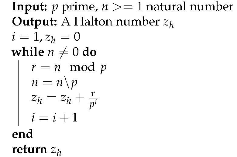 |
The following Halton sequences of Table 5 are constructed according to Algorithm 1 that uses a prime number as its base.
Remark 4.
To generate the n-th Halton point in a sequence consider the base ary expansion of a where the ary coefficients Then the n-th Halton point is It’s easy to build a Halton-sequence with the following observation: If then else if then where (details see [21]). This method is very efficient and will be used in this paper.
5.2. Notation
We use the following notation
| Name | Meaning | ||
| = | = | 0 | |
| = | = | 0 | |
| = | = | 0 | |
| = | = | 0 | |
| = | = | 0 |
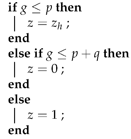
The notation means and the number z is simulated with the following distribution
We generate a pseudorandom number to decide, that values take z, see Algorithm 2.
| Algorithm 2:Simulation of z with distribution (35) |
 |
In Model B (Section 5) we will investigate the class of problems with the condition
If this condition is not satisfied, the problem is easily solved with Model A (Section 4).
5.3. Simulation
The simulation is based on the following lemma.
Lemma 1.
Let and Then
Proof.
The proof proceeds by induction on t. In fact, if because and , we can choose such that .
By induction hypothesis
Then we can choose such that □
Remark 5.
If in Lemma 1 then production in period t is because production up to period satisfies demand up to period t.
Remark 6.
Lemma 1 gives the following lower bound for the production of the products
5.4. Basis of the Simulation
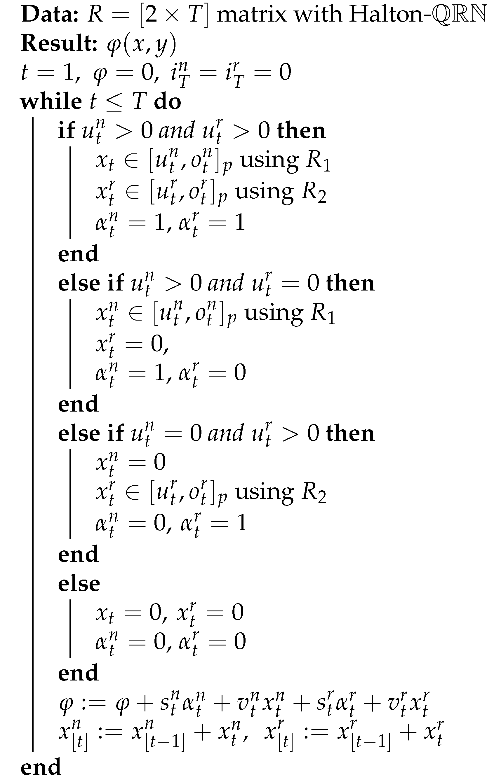
The production plan is created step by step starting from period . To determine the production in period t, we know the selected production until period . In each period, using the constraints of the task (16)-(24) for the production of the products, we determine a lower and an upper bound. Then the production quantity is chosen randomly between the lower and upper limits. These production quantities affect the lower and upper bounds of the future period. We continue in this way until the period . Then we calculate the value of the cost function( i.e. objective function). We repeat this procedure (N times) and choose the production plan with the lowest cost. The advantages of this method, we do not have to worry about the inventory, production or setup costs. The method is now presented in more detail.
Proposition 1.
If then else
Proof.
From (17) we get
If then total production of new products up to period satisfies total demand up to period t and therefore nothing is produced in period i.e. .
If then the production has a lower bound. From (40) we obtain
□
Proposition 2.
If then else and
Proof.
From (18) and (19)
If , then total production up to period satisfies total demand up to period t and therefore nothing is produced in period i.e. .
If then the production has an upper and lower bound. From (43) results the assertion. □
Proposition 3.
If and then
And
Proof.
From (20) and Remark 6
From (2)
From From (46) and (47)
Therefore we simulate the production according to (35)
From (20) using of (49) we get
and then from (2) we obtain
From (50), (51) and (42) results
Therefore we simulate the production according to (35)
□
5.5. Simulation of the Objective Function
Let R be a matrix with Halton’s
We simulate the production starting in period t=1. The calculation of the objective function is carried out with Algorithm 3 using proposition (1), (2) and (3)..
| Algorithm 3:Calculation of the objective function |
 |
Remark 7.
- The generation of the matrix requires operations.
- Die evaluation of the function with Algorithm 3 requires operations
Then, the computational complexity of the simulation with N points and T periods is
6. Numerical Experiments
6.1. Test Design
We analyse the quality of our solution approach of model A and model B by defining 11 problem classes (PC) by varying the number of periods, see Table 6. The planning horizon T is made very large because in the paper industry planning is done daily. Each PC consists of 200 test instances (TI). In model A, 1824 of the 2200 TI were solvable, in model B 2200. In total, we examined 4024 TI. Model A and Model B are implemented on a computer with , ,.
We vary different parameters to define the TI, e.g., the time between orders (TBO) to determine setup costs. The specifications of the parameters are designed in an exaggerated form, which may not occur in practice, to make the TI as difficult as possible.
The parameters for generating data sets (see Table 7) use the following notation where is a random number, that means the values are uniformly distributed on the interval
6.2. Model A
We randomly generate capacities , then with condition (1) randomly generate aggregate demand . This latter is then randomly cut into and . The remaining parameters according to Table 7.
6.2.1. Results of Model A
The solution of problem (25)-(33) (TD) and the optimal solution of problem (16)-(24) (OP) were found with the Gurobi solver version 9.0.3.
We randomly generated 200 instances per PC and usually between 10 and approx. 20% of the instances have no solution (see line Count). This justifies the fact that the problem is not standard. For example, in Table A1 we see that of the 200 instances for problem class , only 167 had a solution.
With the following notation, we can better understand the results of Table A1.
| T | |
| m | |
| solution of problem (25)-(33) | |
| solution of problem (16)-(24) | |
In Table A1 the relative error for Total costs (Tc) and CPU-time for every problem class was calculated as
This is exactly how we calculated the relative errors in inventory cost and setup cost.
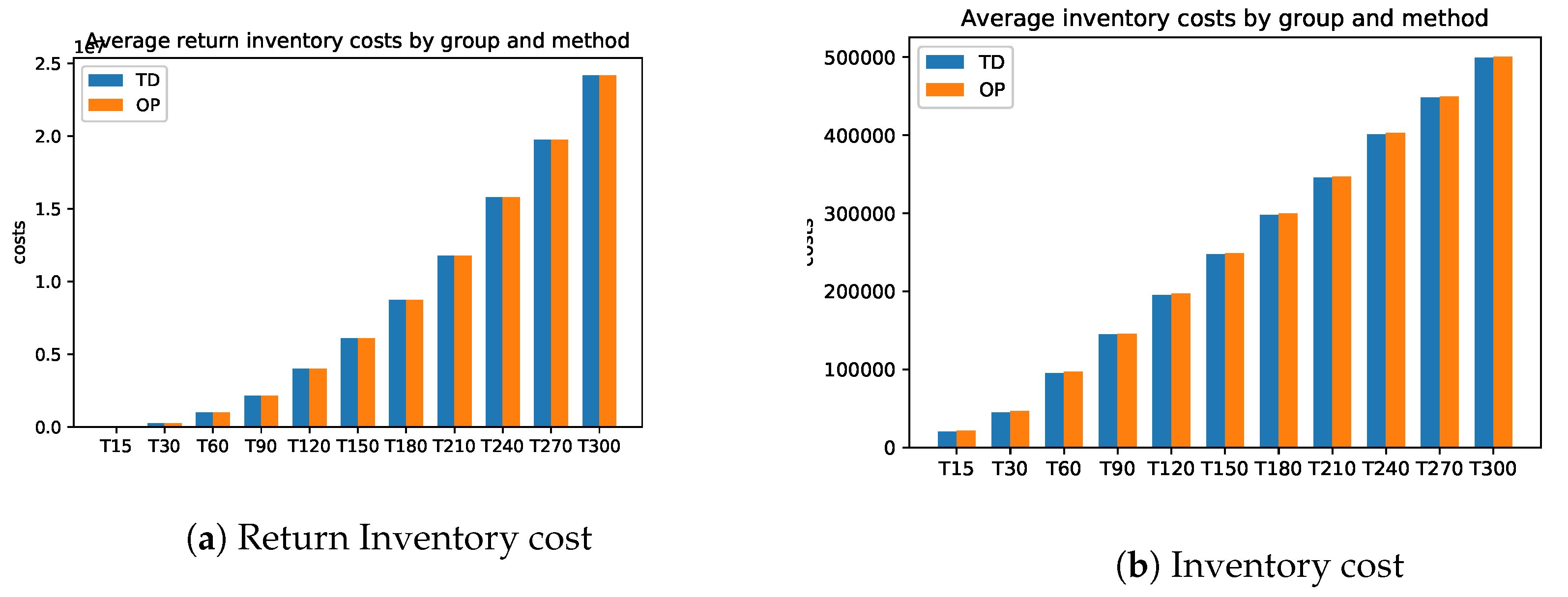
Attached in Appendix A are the results of the average total cost, average CPU time, average Inventory costs
There is hardly any difference between the cost of relaxation (TD) and the original task (OP). Only the computation time for relaxation is faster. The longer the planning horizon, the smaller the difference between the optimal solutions of the problems TD and original optimization task OP. This feature applies to the stocks of the return and setup costs too. On the other hand, the inventory costs for problem TD are always smaller than the inventory costs of problems OP. For more details, please see Figure A1 and Appendix A.1 for the exact calculations. However, we see beyond doubt that this class of problems can be solved very well either with the relaxation TD or directly with a standard solver (here Gurobi).
6.3. Model B
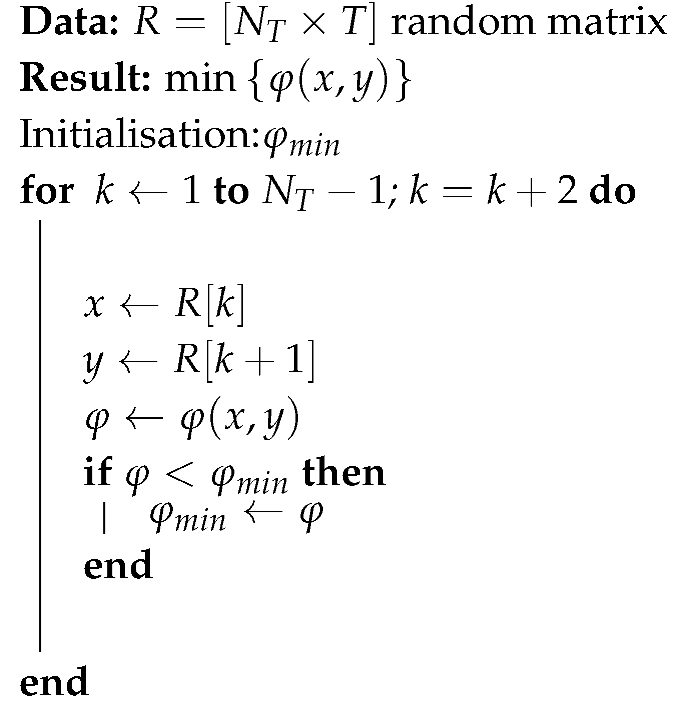
[13] have shown that several families of CLSP are Np-hard. For the construction of the Np-hard instances (2200 instances) we follow the findings of [14]. They use the following notation , where and specify respectively the number of items, a special structure for the setup costs, the holding costs, production costs, and capacities. In this paper [14] they show that the following class 2/C/G/A/C is NP-hard. For this reason we have created 2200 instances, where the set-up costs per product and capacities per instance are constant. The holding cost do not necessarily follow a specified pattern, the production costs can be chosen arbitrarily. The maximum calculation time for Gurobi is 600 seconds. The heuristic operates according to the number of simulations, which gradually increases with the number of periods. The largest group T300 uses 130 seconds. The parameters for generating data sets (see Table 8) use the following notation where is a random number, that means the values are uniformly distributed on the interval
The important assumption in model B is: the capacities for each TI is constant, the set-up costs in each TI and for each product are constant. These parameters vary between a minimum and a maximum depending on the T parameter.
The capacities for each TI vary according to the parameter T. For example if the capacities are between 600 and 800. If the capacities vary between 3000 and 5500. Analogously the other parameters. The remaining parameters according to Table 8.
For the simulation we used following parameters:
is the Halton’s numbers used for T periods (see Table 9).
All instances for have the same schema Step 1 until Step 5. We used (see Table 10).
| Algorithm 4:Heuristic: blind search |
 |
6.3.1. Results of Model B
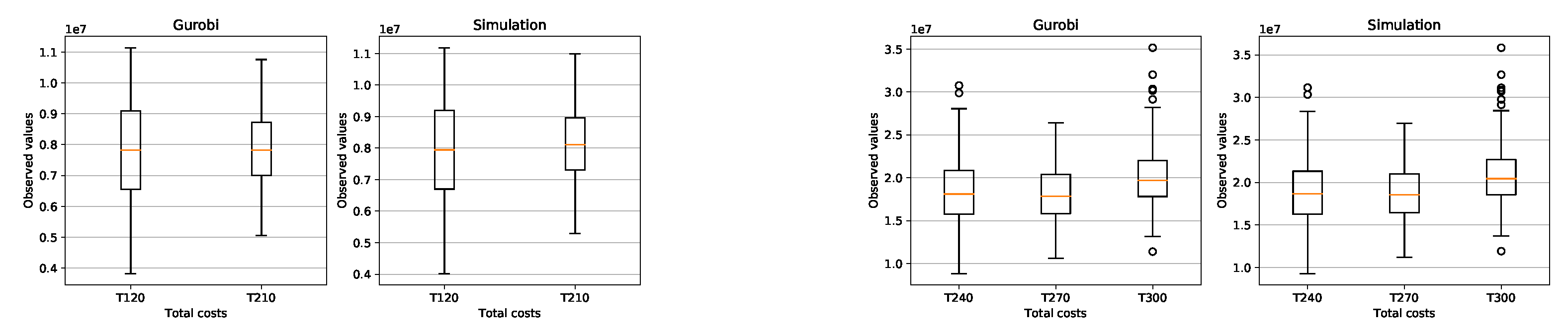
We generated 200 random instances for each problem class (PC) and with a Box-plot we compared the feasible solutions of the problem (16)-(24) found by Gurobi 9.0.3 with the solution of the simulation presented in this paper and clearly see the similarity of the results found (see Figure A4 and Figure A5).
With the following notation we present the results (see Table A3).
| T | |
| m | |
| with Simulation | |
| with Gurobi |
In Table A3 the relative error for Total costs (Tc) and CPU-time for every problem class was calculated as
The graphical comparison is shown in Figure A3.
This is exactly how we calculated the relative errors in inventory cost and setup cost. Attached in Appendix B are the results of the average total cost, average CPU time, average Inventory costs. Figure A3 (average CPU time) clearly shows that the Gurobi admissible solution for the PC from T150 to T300 are not optimal and that the CPU of the simulation is much faster.
The simulation in average determines the setup costs and return inventory costs always higher than Gurobi. On the other hand, the inventory costs of Gurobi are higher than the simulation. What can we say about the quality of the solution of the problems? the simulation could not give a better solution than Gurobi’s solution. Gurobi solved the (PC) problems up to T120 in an optimal way. The problems from T150 to T300 were not solved optimally by Gurobi, since it would take too much time due to the Np-hard category of the problem. The simulation found feasible solutions much faster than Gurobi. Here is the advantage of the simulation, the simplicity of its implementation and the speed in finding an acceptable solution.
7. Conclusions and Outlook
We have analyzed a problem that belongs to the NP-hard class. However, the choice of the parameters is very important to obtain a problem that is really Np-hard. With the choice of parameters made in model A, we see that this class of problems is easily solved with a standard solver. By doing a relaxation of the problem, the solution is found more quickly. The error rate is between 0.02% and 2% (taking into account more than 1800 instances).
If we choose the parameters according to model B, Gurobi needs a lot of time to find the optimal solution. In this kind of problem the presented simulation can help a lot in finding a good solution. We have seen that the error rate is between 1.7% and 3.5% (taking into account more than 2000 instances). The simulation is sometimes better than Gurobi, but on average Gurobi solves the problem with a maximum time of 600 seconds better than the simulation. The great advantage of the simulation is that the calculation is extremely fast and easy.Thanks to the Halton numbers, few simulations are needed to obtain a very good approximation of the solution.
The simulation has a general character and can be adapted to investigate even more complex problems of the Np-hard category ( for example, researching CLSP problems with n products).
The quality of the solutions can be improved by increasing the number of simulations but it is necessary to have a fairly fast computer. In this work we use at most 10 million simulations. Another parameter that influences the quality of the solutions is the correct choice of the probability p (see (35)). Is there an optimal probability? This is a question for further research.
Acknowledgments
My special thanks to Luis Aurelio Rocha of Passau University for his comments on this work.
Abbreviations
The following abbreviations are used in this manuscript:
| Low-discrepancy sequences, also known as Quasirandom sequences, | |
| CLSP | capacitated lot-sitzing problem |
Appendix A. Results Visualization
Appendix A.1. Model A
Figure A1.
Model A: Average Totalcost and CPU Time.
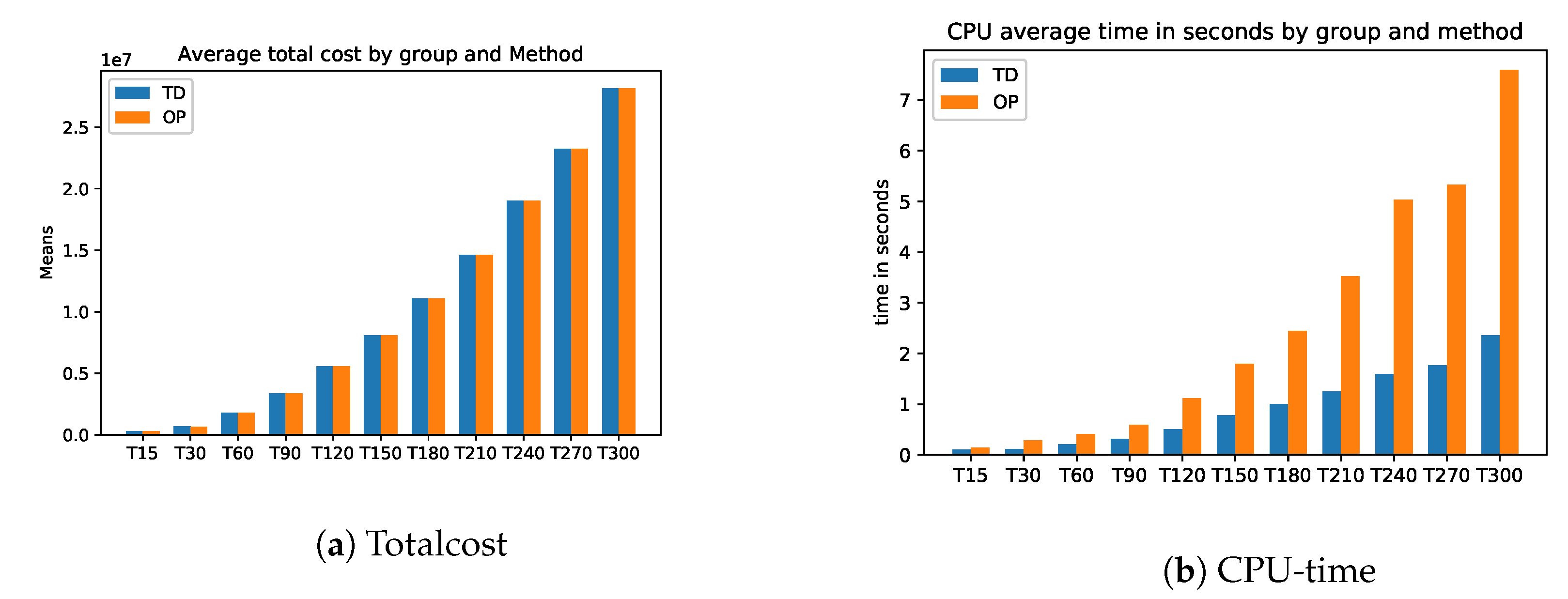
Figure A2.
Model A: Average Inventory cost.
Appendix A.2. Model B
Visualization of the results and average costs.
Figure A3.
Model B: Average Total cost and CPU time.
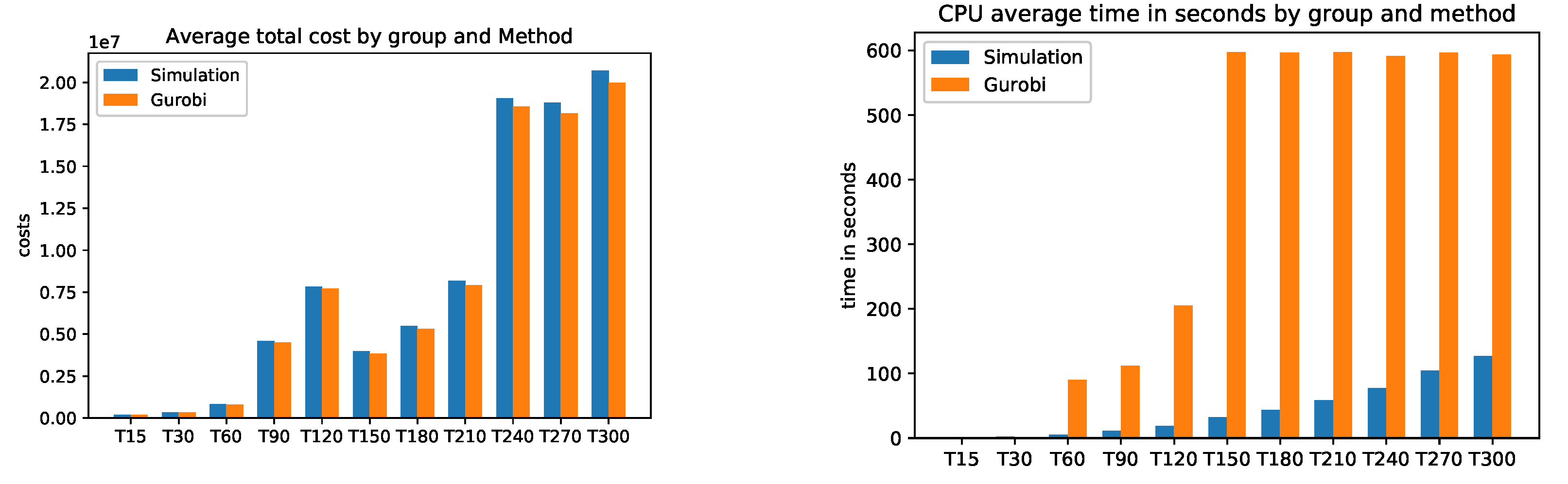
Figure A4.
Model B: Total costs.
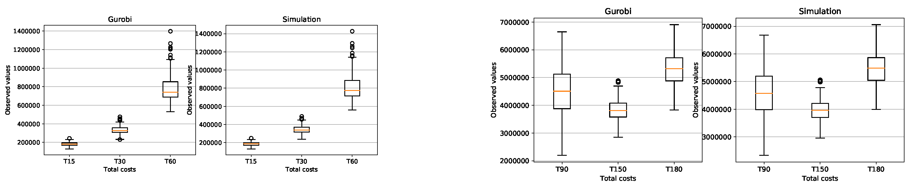
Figure A5.
Model B: Total costs.
Appendix B. Average Costs
Appendix B.1. Model A
Table A1.
Model A: Average Total Costs.
| Total Costs | T | 15 | 30 | 60 | 90 | 120 | 150 |
|---|---|---|---|---|---|---|---|
| Count | 172 | 155 | 167 | 162 | 166 | 164 | |
| TD | Mean | 274061 | 665537 | 1798127 | 3348945 | 5552436 | 8062797 |
| Std. | 87161 | 151370 | 389288 | 660684 | 906092 | 1349699 | |
| Optimal | Mean | 268593 | 659453 | 1792494 | 3344788 | 5546715 | 8058311 |
| Std. | 83431 | 148783 | 385859 | 659403 | 904686 | 1348457 | |
| Relative error | Tc | 2,04% | 0,92% | 0,31% | 0,12% | 0,10% | 0,06% |
| Total costs | T | 150 | 180 | 210 | 240 | 270 | 300 |
| Count | 164 | 164 | 168 | 168 | 170 | 168 | |
| TD | Mean | 8062797 | 11087631 | 14620895 | 19015245 | 23243458 | 28160753 |
| Std. | 1349699 | 1811439 | 2199306 | 2911556 | 3384673 | 3870830 | |
| Optimal | Mean | 8058311 | 11081145 | 14614610 | 19008049 | 23237758 | 28154353 |
| Std. | 1348457 | 1808995 | 2198938 | 2910200 | 3382841 | 3868995 | |
| Relative error | Tc | 0,06% | 0,06% | 0,04% | 0,04% | 0,02% | 0,02% |
Table A2.
Model A: Average CPU time.
| CPU Time | T | 15 | 30 | 60 | 90 | 120 | 150 |
|---|---|---|---|---|---|---|---|
| Count | 172 | 155 | 167 | 162 | 166 | 164 | |
| TD | Mean | 0,10 | 0,11 | 0,21 | 0,31 | 0,50 | 0,78 |
| Std. | 0,06 | 0,05 | 0,10 | 0,16 | 0,26 | 0,39 | |
| Optimal | Mean | 0,14 | 0,28 | 0,41 | 0,59 | 1,12 | 1,79 |
| Std. | 0,06 | 0,11 | 0,17 | 0,30 | 0,51 | 1,42 | |
| Relative error | CPU | -25,27% | -59,97% | -49,61% | -47,53% | -55,39% | -56,26% |
| CPU Time | T | 150 | 180 | 210 | 240 | 270 | 300 |
| Count | 164 | 164 | 168 | 168 | 170 | 168 | |
| TD | Mean | 0,78 | 1,00 | 1,25 | 1,59 | 1,77 | 2,36 |
| Std. | 0,39 | 0,47 | 0,69 | 0,82 | 0,90 | 1,39 | |
| Optimal | Mean | 1,79 | 2,44 | 3,52 | 5,03 | 5,33 | 7,60 |
| Std. | 1,42 | 1,73 | 3,00 | 3,50 | 3,98 | 5,97 | |
| Relative error | CPU | -56,26% | -59,00% | -64,53% | -68,46% | -66,87% | -68,94% |
Appendix B.2. Model B
Table A3.
Model B: Average Total Costs.
| Total Costs | T | 15 | 30 | 60 | 90 | 120 | 150 |
|---|---|---|---|---|---|---|---|
| Count | 200 | 200 | 200 | 200 | 200 | 200 | |
| Simulation | Mean | 185971 | 342933 | 815220 | 4576352 | 7829443 | 3979678 |
| Std. | 21273 | 45909 | 155884 | 858442 | 1559305 | 397507 | |
| Gurobi | Mean | 182040 | 332163 | 784654 | 4498331 | 7718552 | 3845522 |
| Std. | 21125 | 45150 | 155097 | 882996 | 1594738 | 393440 | |
| Relative error | Tc | 2,16% | 3,24% | 3,90% | 1,73% | 1,44% | 3,49% |
| Total costs | T | 150 | 180 | 210 | 240 | 270 | 300 |
| Count | 200 | 200 | 200 | 200 | 200 | 200 | |
| Simulation | Mean | 3979678 | 5477237 | 8177244 | 19065355 | 18786745 | 20708665 |
| Std. | 397507 | 593444 | 1275892 | 4030464 | 3201422 | 3672141 | |
| Gurobi | Mean | 3845522 | 5318346 | 7905438 | 18570461 | 18146172 | 19992493 |
| Std. | 393440 | 590176 | 1265172 | 4055425 | 3179322 | 3670651 | |
| Relative error | Tc | 3,49% | 2,99% | 3,44% | 2,66% | 3,53% | 3,58% |
Table A4.
Model B: Average CPU time.
| CPU Time | T | 15 | 30 | 60 | 90 | 120 | 150 |
|---|---|---|---|---|---|---|---|
| Count | 200 | 200 | 200 | 200 | 200 | 200 | |
| Simulation | Mean | 0,79 | 2,28 | 5,94 | 11,68 | 19,87 | 34,12 |
| Std. | 0,13 | 0,13 | 0,16 | 0,18 | 0,23 | 0,54 | |
| Gurobi | Mean | 0,12 | 1,57 | 90,38 | 111,93 | 204,94 | 597,03 |
| Std. | 0,08 | 1,53 | 156,10 | 186,04 | 245,47 | 36,02 | |
| Relative error | CPU | 552,92% | 44,87% | -93,43% | -89,56% | -90,31% | -94,28% |
| CPU Time | T | 150 | 180 | 210 | 240 | 270 | 300 |
| Count | 200 | 200 | 200 | 200 | 200 | 200 | |
| Simulation | Mean | 34,12 | 46,26 | 62,84 | 77,96 | 101,69 | 130,17 |
| Std. | 0,54 | 0,58 | 1,22 | 2,63 | 2,74 | 3,78 | |
| Gurobi | Mean | 597,03 | 596,88 | 597,47 | 591,51 | 596,54 | 593,22 |
| Std. | 36,02 | 4,06 | 3,92 | 33,19 | 3,80 | 7,14 | |
| Relative error | CPU | -94,28% | -92,25% | -89,48% | -86,82% | -82,95% | -78,06% |
Table A5.
Model B: Inventory costs.
| Inventory Costs | T | 15 | 30 | 60 | 90 | 120 | 150 |
|---|---|---|---|---|---|---|---|
| Count | 200 | 200 | 200 | 200 | 200 | 200 | |
| Simulation | Mean | 28307 | 52842 | 112536 | 253095 | 340599 | 260657 |
| Std. | 5341 | 8170 | 12391 | 86118 | 107587 | 28744 | |
| Gurobi | Mean | 27801 | 57117 | 132943 | 509248 | 790970 | 318360 |
| Std. | 6907 | 12243 | 29889 | 194930 | 324335 | 43350 | |
| Relative error | Inv. | 1,82% | -7,49% | -15,35% | -50,30% | -56,94% | -18,13% |
| Inventory costs | T | 150 | 180 | 210 | 240 | 270 | 300 |
| Count | 200 | 200 | 200 | 200 | 200 | 200 | |
| Simulation | Mean | 260657 | 345666 | 542344 | 990715 | 1147482 | 1282444 |
| Std. | 28744 | 38613 | 75292 | 175805 | 161861 | 196713 | |
| Gurobi | Mean | 318360 | 507104 | 835915 | 1859977 | 1730800 | 1959659 |
| Std. | 43350 | 89630 | 191367 | 486708 | 372666 | 455506 | |
| Relative error | Inv. | -18,13% | -31,84% | -35,12% | -46,74% | -33,70% | -34,56% |
Table A6.
Model B: Return stock cost.
| Return Inventory Costs | T | 15 | 30 | 60 | 90 | 120 | 150 |
|---|---|---|---|---|---|---|---|
| Count | 200 | 200 | 200 | 200 | 200 | 200 | |
| Simulation | Mean | 45867 | 92667 | 249888 | 3690209 | 6646915 | 821946 |
| Std. | 18040 | 35850 | 137395 | 1028216 | 1793396 | 208315 | |
| Gurobi | Mean | 41356 | 74641 | 195294 | 3346068 | 6070949 | 700634 |
| Std. | 17493 | 33456 | 133042 | 1109603 | 1957840 | 207573 | |
| Relative error | Ret. Inv. | 10,91% | 24,15% | 27,96% | 10,28% | 9,49% | 17,31% |
| Return Inventory costs | T | 150 | 180 | 210 | 240 | 270 | 300 |
| Count | 200 | 200 | 200 | 200 | 200 | 200 | |
| Simulation | Mean | 821946 | 1548362 | 2628642 | 9347966 | 7251886 | 8608929 |
| Std. | 208315 | 482657 | 1041268 | 4406311 | 2744151 | 3706917 | |
| Gurobi | Mean | 700634 | 1293559 | 2169556 | 8142232 | 6309891 | 7524531 |
| Std. | 207573 | 477084 | 1026872 | 4293352 | 2685984 | 3610684 | |
| Relative error | Ret. Inv. | 17,31% | 19,70% | 21,16% | 14,81% | 14,93% | 14,41% |
Table A7.
Model B: Average Setup costs.
| Setup Costs | T | 15 | 30 | 60 | 90 | 120 | 150 |
|---|---|---|---|---|---|---|---|
| Count | 200 | 200 | 200 | 200 | 200 | 200 | |
| Simulation | Mean | 50033 | 106876 | 238570 | 293071 | 388685 | 1521814 |
| Std. | 10663 | 17638 | 31424 | 27563 | 34664 | 212705 | |
| Gurobi | Mean | 55707 | 114588 | 248504 | 307481 | 408104 | 1458747 |
| Std. | 10343 | 17268 | 30443 | 27399 | 37230 | 201433 | |
| Relative error | Setup | -10,19% | -6,73% | -4,00% | -4,69% | -4,76% | 4,32% |
| Setup Costs | T | 150 | 180 | 210 | 240 | 270 | 300 |
| Count | 200 | 200 | 200 | 200 | 200 | 200 | |
| Simulation | Mean | 1521814 | 1699197 | 2214098 | 2828660 | 3716988 | 4920930 |
| Std. | 212705 | 233148 | 330991 | 404730 | 467555 | 902775 | |
| Gurobi | Mean | 1458747 | 1641182 | 2118141 | 2669355 | 3397775 | 4526298 |
| Std. | 201433 | 223689 | 310292 | 367954 | 412785 | 200 | |
| Relative error | Setup | 4,32% | 3,53% | 4,53% | 5,97% | 9,39% | 8,72% |
References
- Thierry, M.; Salomon, M.; Van Nunen, J.; Van Wassenhove, L. Strategic issues in product recovery management. California Management Review 1995, 37, 114–135. [Google Scholar] [CrossRef]
- Umweltbundesamt. Papier und Druckerzeugnisse, 2020.
- Sahling, F. A Column-Generation Approach for a Short-Term Production Planning Problem in Closed-Loop Supply Chains. BuR- Business Research 2016, 6, 55–75. [Google Scholar] [CrossRef]
- Helmrich, R.; Jans, M.; van den Heuvel, W.; Wagelmans, A. Economic lot-sizing with remanufacturing: Complexity and efficient formulations. IISE Transactions 2014, 46(1), 67–86. [Google Scholar] [CrossRef]
- Sifaleras, A.; Konstantaras, I. Variable neighborhood descent heuristic for solving reverse logistics multi-item dynamic lot-sizing problems. Electronic Notes in Discrete Mathematics 2015, 47, 69–76. [Google Scholar] [CrossRef]
- Kilic, O.; van den Heuvel, W. Economic lot sizing with remanufacturing: Structural properties and polynomial-time heuristics. IISE Transactions 2019, 51, 1318–1331. [Google Scholar] [CrossRef]
- Richter, K.; Weber, J. Thre reverse Wagner/Whitin model with variable manufacturing and remanufacturing cost. International Journal of Production Economics 2001, 71, 447–456. [Google Scholar] [CrossRef]
- Richter, K.; Sombrutzki, M. Remanufacturing planing for the reverse Wagner/Whitin models. Journal of Operational Research 2000, 121, 304–315. [Google Scholar] [CrossRef]
- Teunter, R.; Bayindir, Z.; van den Heuvel, W. Dynamic lot sizing with product returns and remanufacturing. Int. Journal of Production Research 2006, 4377–4400. [Google Scholar] [CrossRef]
- Schulz, T. A new Silver-Meal basic heuristic for the single-item dynamic lot sizing problem with returns and remanufacturing. International Journal of Production Research 2011, 2519–2533. [Google Scholar] [CrossRef]
- Cunha, J.; Melo, R. A computational comparison of formulations for the economic lot-sizing with remanufacturing. Computers & Industrial Engineering 2016, 92, 72–81. [Google Scholar]
- Zhang, Z.; Jiang, H.; Pan, X. A lagrangian relaxation based approach for the capacitated lot sizing problem in closed-loop supply chain. Int. J. Productions Economics 2012, 140, 249–255. [Google Scholar] [CrossRef]
- Florian, M.; Lenstra, J.; Rinnooy, K. Deterministic production planning algorithms and complexity. Management Science 1980, 26, 669–679. [Google Scholar] [CrossRef]
- Bitran, G.; Yanasse, H. Computational complexity of the capacitated lot size problem. Management Science 1982, 28, 1174–1186. [Google Scholar] [CrossRef]
- Dixon, P. Multi-Item Lot-Sizing with Limited Capacity. dissertation, University of Waterloo, Ontario, 1979.
- Karimi, B.; Fatemi Ghomi, S.; Wilson, J.M. The capacitated lot sizing problem review of models and algorithms. OMEGA 2003, 31, 365–378. [Google Scholar] [CrossRef]
- Maes, J.; McClain, J.; Van Wassenhove, L. Multilevel capacitated lotsizing complexity and LP-based heuristics. Journal of Operational Research 1991, 53, 131–148. [Google Scholar] [CrossRef]
- Sobol, I. Calculation of improper integrals using uniformly distributed sequences. Soviet Math. Dokl. 1973, 14, 734–738. [Google Scholar]
- Halton, J.H. On the efficiency of certain quasi-random sequences of points in evaluating multi-dimensional integrals. Numer. Math. 1960, 2, 84–90. [Google Scholar] [CrossRef]
- Niederreiter, H. Quasi-Monte Carlo methods and pseudo-random numbers. Bull. Am. Math. Soc. 1978, 84, 957–1041. [Google Scholar] [CrossRef]
- Klinger, B. Numerical Integration of Singular Integrands using Low-Discrepancy Sequences. Computing 1997, 59, 223–236. [Google Scholar] [CrossRef]
- Heuvel, W.; Wagelmans, A. Four equivalent lot-sizing models. Operations Research Letters 2008, 36, 465–470. [Google Scholar] [CrossRef]
- Maes, J.; Van Wassenhove, L. A simple heuristic for the multi item single level capacitated lotsizing problem. Operations research letters 1986, 4, 265–273. [Google Scholar] [CrossRef]
- Knuth, D.E. The Art of Compute Programming: Seminumerical Algorithms. Volume 2.; Addison-Wesley, 1981.
- von Neumann, J. Various techniques used in connection with random digits. Monte Carlo Method, Appl. Math. Series 1951, 12, 36–38. [Google Scholar]
- Niederreiter, H. Random Number Generation and Quasi-Monte Carlo Methods.; SIAM, 1992.
- Tezuka, S. Uniform Random Numbers: Theory and Practice.; Kluwer Academic, 1995.
- Chaitin, G. Information, Randomness and Incompleteness. Papers on Algorithmic Information Theory. 1987, p. 236.
- Kolmogorov, A.; Uspenskii, V. Algorithms and randomness. Teor. Veroyatnost i Primenen. 1987, 32, 425–455. [Google Scholar] [CrossRef]
- Schnorr, C. Zufälligkeit und Wahrscheinlichkeit. Lecture Notes in Math. 1971, 218, 109. [Google Scholar]
Figure 1.
Dynamic Capacitated Lot-Sizing with Produkt Returns and Remanufacturing.
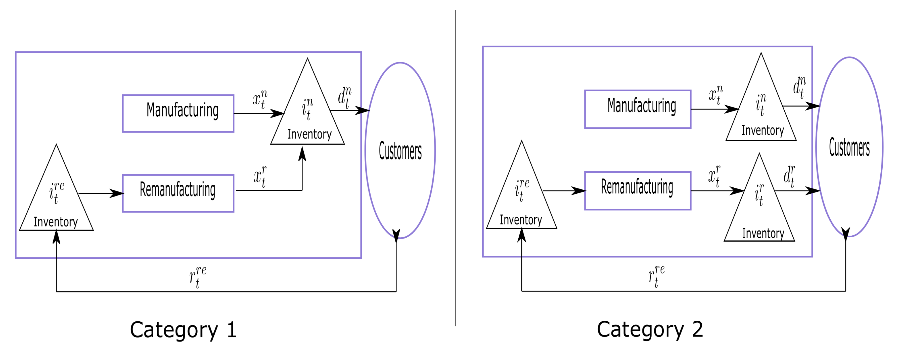
Figure 2.
Two-dimensional projection of 5000 Halton and Pseudorandom points.
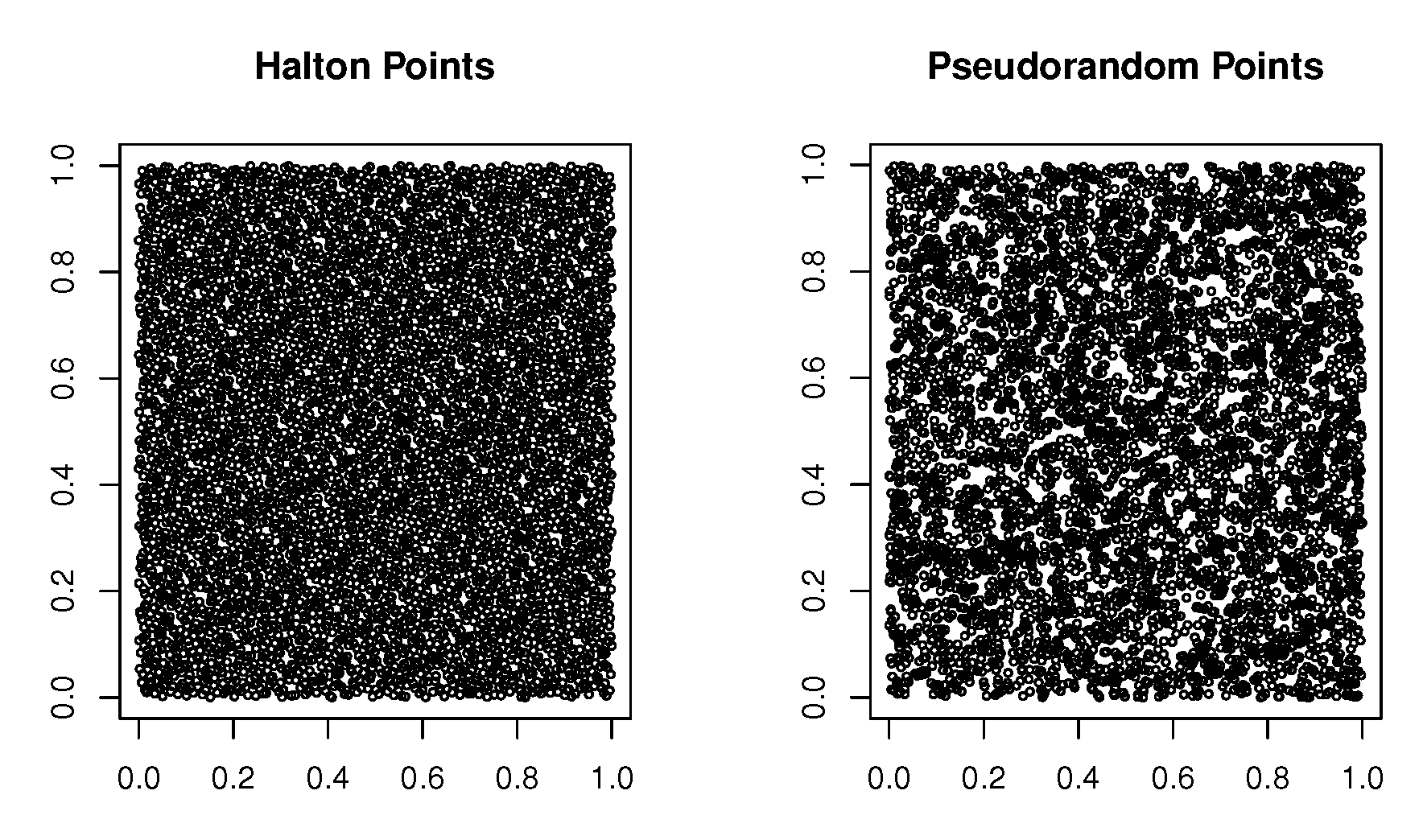
Table 1.
Data and parameters.
| Name | Paramenter |
|---|---|
| T | Number of time periods |
| Initial inventory stocks | |
| Cost per unit and period t | |
| Setup cost for manufacturing new product | |
| Setup cost for remanufacturing product | |
| production cost of new product | |
| production cost of remanufactured product | |
| holding cost of new product | |
| holding cost of remanufactured product | |
| holding cost of returned product | |
| Demand and return in period t | |
| Demand of new product | |
| Demand of remanufactured product | |
| Quantity of returned product | |
| Available Capacities in period t | |
| capacities for manufacturing and | |
| remanufacturing | |
| (capacity requirement for new product and | |
| recovery product is set to one). | |
Table 2.
Decision variables.
| Name | Paramenter |
|---|---|
| 1, if new products are manufactured | |
| in period t; 0, otherwise | |
| quantity of new products manufactured | |
| in period t | |
| inventory stock of new products | |
| at the end of period t | |
| 1, if returned products are remanufactured | |
| in period t; 0, otherwise | |
| quantity of returned products remanufactured | |
| in period t | |
| inventory stock of remanufactured | |
| products at the end of period t | |
| inventory stock of returned products | |
| at the end of period t |
Table 5.
Halton Numbers.
| Prime Numbers | ||||
|---|---|---|---|---|
| 2 | 3 | 5 | 7 | |
| n | Halton numbers | |||
| 1 | 0,5 | 0,33333333 | 0,2 | 0,14285714 |
| 2 | 0,25 | 0,66666667 | 0,4 | 0,28571429 |
| 3 | 0,75 | 0,11111111 | 0,6 | 0,42857143 |
| 4 | 0,125 | 0,44444444 | 0,8 | 0,57142857 |
| 5 | 0,625 | 0,77777778 | 0,04 | 0,71428571 |
Table 6.
Problem classes.
| PC1 | PC2 | PC3 | PC4 | PC5 | PC6 | |
|---|---|---|---|---|---|---|
| T | 15 | 30 | 60 | 90 | 120 | 150 |
| PC7 | PC8 | PC9 | PC10 | PC11 | ||
| T | 180 | 210 | 240 | 270 | 300 |
Table 7.
Parameters for Model A.
| with condition (1) | |
|---|---|
| with condition (4) | with condition (3) |
| = | |
| = |
Table 8.
Model B: Parameters.
| with condition (1) | |
|---|---|
| with condition (4) | with condition (3) |
Table 9.
Periods, Halton’s numbers.
| T | |
|---|---|
| 15 | 491520 |
| 30 | 983040 |
| 60 | 1966080 |
| 90 | 2949120 |
| 120 | 3932160 |
| 150 | 4915200 |
| 180 | 5898240 |
| 210 | 6881280 |
| 240 | 7864320 |
| 270 | 8847360 |
| 300 | 9830400 |
Table 10.
Schematic of the simulation.
| Step 1 | Initialisation:, |
|---|---|
| Step 2 | If stop; otherwise go to Step 3. |
| Step 3 | Using Algorithm 4 and calculate the function |
| Step 4 | If then . |
| Step 5 | and go to Step 2. |
Disclaimer/Publisher’s Note: The statements, opinions and data contained in all publications are solely those of the individual author(s) and contributor(s) and not of MDPI and/or the editor(s). MDPI and/or the editor(s) disclaim responsibility for any injury to people or property resulting from any ideas, methods, instructions or products referred to in the content. |
© 2023 by the authors. Licensee MDPI, Basel, Switzerland. This article is an open access article distributed under the terms and conditions of the Creative Commons Attribution (CC BY) license (http://creativecommons.org/licenses/by/4.0/).
Copyright: This open access article is published under a Creative Commons CC BY 4.0 license, which permit the free download, distribution, and reuse, provided that the author and preprint are cited in any reuse.