
Submitted:
10 April 2023
Posted:
11 April 2023
You are already at the latest version
Abstract
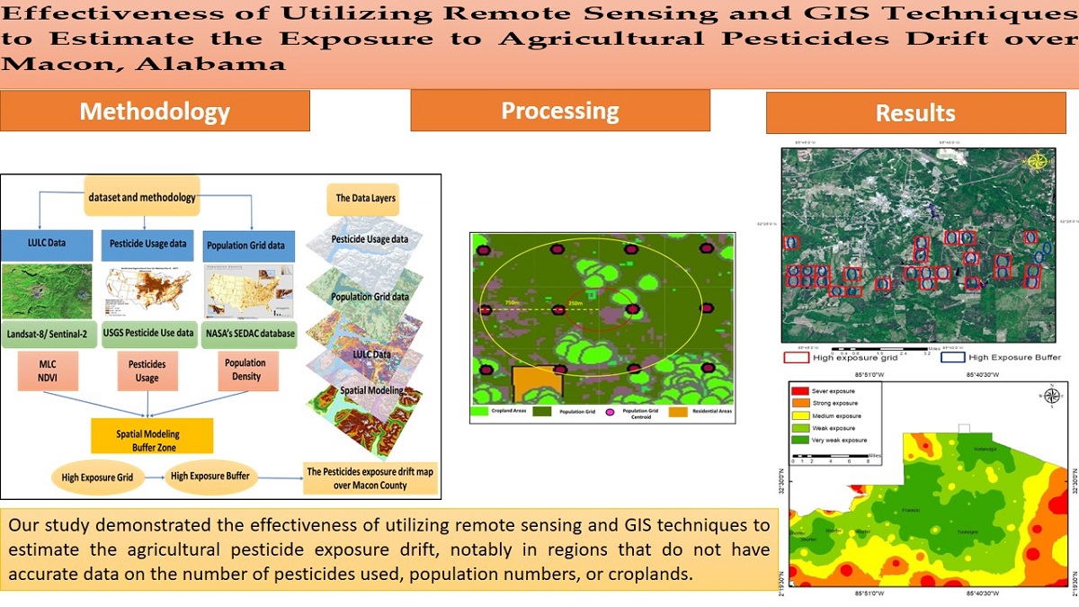
Agricultural workers utilize pesticides extensively on their farms to control weeds and insects, as well as increase crop productivity. Despite these advantages, their excessive use poses a seri-ous threat, particularly to the population living at the nexus of urban and rural areas. Exposure to pesticide drift can be investigated using geospatial tools. Remote sensing technology and Geographic Information Systems (GIS) techniques have been used intensively and constitute trusted tools in different sectors, especially in agriculture. Remote sensing depends on pro-cessing the electromagnetic radiation reflected and emitted from the ground target and can be used to identify the spectral signature of crops exposed to pesticides. GIS has powerful tools for building a spatial geo-database of pesticide exposure drift. Therefore, the major objective of the research was to explore the effectiveness of using remote sensing and GIS techniques to estimate the exposure to pesticides in Macon County (Alabama). To achieve this objective, Maximum Likelihood Classification (MLC) was used to identify accurate cropland areas. The Landsat-8 and Sentinel-2 satellite images. Available agricultural pesticide usage data (seven of the seventeen organophosphates used in Alabama) were obtained through the United States Geological Survey (USGS). The results indicated that 6.6% of Macon County’s residents are considered potentially severely exposed, and the potentially affected population resides primarily in rural areas. While 23 percent of residents of rural edges are considered to have potentially medium to high expo-sure. In addition, 38% of residents living in suburban areas are considered to have potentially low-to-medium exposure. Also, the results indicated that both GIS and remote sensing can play an effective role in estimating pesticide exposure drift.
Keywords:
Agricultural pesticides
; spray drift
; MLC
1. Introduction
Chemical treatments known as pesticides are frequently utilized in agriculture. These substances work to eliminate undesirable organisms, including fungi, weeds, and insects, that could otherwise ruin crops or limit their productivity. Other sectors also use pesticides to destroy exotic plants, remove weeds and shrubs from roads, and limit the formation of algae in water bodies. Pesticides have been heavily utilized in agriculture all over the world to guarantee higher crop yields [1,2,3]. According to the World Atlas 2022, the USA uses 850,984,332 pounds of pesticides annually, making it the second-largest consumer after China [4]. Herbicides account for 40% of pesticide use globally, followed by insecticides at 17% and fungicides at 10% [5]. They are naturally poisonous, making up one of the most dangerous classes of pollutants for flora, animals, and the environment [6].
Short- and long-term exposure to pesticides can cause congestion of the heart, lungs, and kidneys, weight loss, and reproductive effects. Children are predominantly vulnerable to the impacts of pesticide drift due to their age, weight, and development [7]. Previous health studies on pesticide drift have established a relationship between exposure to pesticides in residential areas near agricultural fields and the high number of childhood cancers and brain tumors [8,9,10]. Moreover, exposure to pesticides is associated with adverse reproductive and neurologic/neurobehavioral effects and thyroid dysfunction [11,12,13,14].
Pesticide drift refers to the off-target movement of pesticide droplets during and after treatment. The coarse droplets move over short distances and fall near the launch point. While fine particles can remain suspended in air currents for prolonged periods and be carried away from the target areas to their adjacent ones. As a result, pesticide drift has become an increasingly debatable issue at the urban-rural margins and affects social justice, especially concerning quality of life [15]. It is widely confirmed that farmers and communities surrounding agricultural areas are the most at-risk groups for pesticide drift. However, applicators are always the most vulnerable to pesticide application, due to insufficient protection, droplet drift, leaks, and other defects in spraying equipment [16].
Pesticide drift exposure is usually classified into two categories based on the type of application: occupational and non-occupational exposure drift. Occupational exposure drift occurs during pesticide spraying in pesticide users and their immediate family members, farmers, and applicators [17].
While non-occupational pesticide exposure occurs in residential areas and around water bodies near pesticide application locations, where chemicals drift from 50 m to 2 km within residential areas and human activity centers, depending on the type of treatment, whether ground, orchards, or aerial application. Despite the significant impacts of pesticide exposure drift on population and health conditions, there have only been a few research studies that have measured non-occupational exposure drift; this is due to being constrained by detailed pesticide source data and measuring drift exposure applications on a local scale [18,19].
To estimate the agricultural pesticide drift impacts, it is vital to acquire detailed data concerning the pesticide labels and application type and to determine the buffer zone between the cropland and the nearest residential area. This study is primarily concerned with measuring non-occupational exposure drift because its negative effects on residential areas and water bodies are greater than those from occupational exposure. Therefore, assessing agricultural pesticide exposure drift at the county level is of utmost importance from meteorological, health, and environmental perspectives.
Monitoring the concentrations of pesticides in the atmosphere is one of the research issues worth studying, due to the significant impact on the drift of insecticides from their target, and modern techniques face many difficulties in this type of complex study. It is recognized that satellite images are used to determine land use and land cover due to the dependence on those satellites for monitoring and measurement at different radiometric, spectral, spatial, and temporal resolutions. These satellite images can be obtained free of charge from the US Geological Survey website (https://earthexplorer.usgs.gov/). Landsat satellite images allow researchers to create an innovative opportunity to study the impact of exposure to pesticide drift from the target, especially in agricultural areas where ground measurements are not available, such as Macon County in Alabama [20,21].
Controlling studies concerning pesticides and human beings is far more complex due to the myriad factors that influence human disease and health. There are countless classes and types of pesticides on the market, all of which interact with organisms differently, making studies on pesticides all the more daunting due to the massive number of pesticides on the market.
It is worth mentioning that we found some studies around the US that described ways to analyze exposure to environmental pesticides using modern techniques. They mainly monitored the possibility of using modern techniques to calculate quantities of agricultural pesticides applied in the vicinity of a residential site as a proxy for non-food exposures. Marusek [22] and Ritz [23] focused on the surrounding agricultural land using GIS. Nuckols [24], Ward [25] and Teysseire [26] used the dwelling distance from the fields, but they took into account the possibility of obstacles such as forests and trees.
Previous studies have utilized remote sensing and GIS techniques to study the impact of pesticide exposure drift on the community and environment, particularly in counties without a record of pesticide use. Hence, their methods and findings will be more beneficial at the county level, such as in Macon County. Dappen [27] used the supervised classification technique using GIS to create a land use land cover map. It was created on a large scale for the 2005 growing season so that it could be developed to include the entire state of Nebraska. Moreover, Wang [28] created a model for assessing the potential spray drift in off-croplands. The study concluded that spray drift can be simulated and estimated according to the application type and the buffer zone range from the unintended targets.
Notably, previous research supported the idea that pesticide exposure drift might be estimated by combining population, and land use land cover data with standard pesticide usage data. Wan [29] provided an overview of potential pesticide exposure without detailed pesticide usage data in Nebraska. His methodology examines the acreage of corn and soybeans within a 450-m buffer zone from a population centroid to determine the possible population in Madison County exposed to pesticide drift. Wan utilized county-wide USGS pesticide usage estimates, which are calculated by a survey. He used census data, available pesticide data, and land use land cover data. He overlaid them all as layers in GIS.
Wan conducted a weighted pesticide exposure study and found that 12% of Nebraska residents were at risk due to exposure to pesticide drift. Brouwer [30] created a spatiotemporal model to estimate potential environmental exposure to individual pesticides in the Netherlands as part of an ongoing case-control study on Parkinson’s disease. Ann Myers [31] assessed the potential population in Madison County exposed to pesticide drift, which is accomplished by examining the amount of cotton, corn, and soybean within a 450-m buffer zone from a population centroid. A quick inspection of previous studies reveals that there are no attempts to conduct studies related to an estimate of the agricultural pesticides’ exposure drift over Macon, Alabama. Particularly in the sense of the concurrent rural and urban population exposure to pesticide drift.
Overall, based on available studies, it can be noted that most of them were not spatially evenly distributed in the United States, and many US states did not receive adequate study, despite the significance of understanding how pesticide use affects residential areas, applicators, and the environment. This is a result of the scarcity of pertinent data, particularly for the state of Alabama, which is needed for further study. Recalling all these challenges, the utilization of agricultural pesticides in Alabama has raised the risk of pesticide drift, particularly when more people live on agricultural land and are exposed to more chemicals. According to estimates, Macon County used 3.89 kg/ha of pesticides in 2021, which is more than the global average of 2.63 kg/ha [32,33].
Therefore, the major purpose of this study is to assess the effectiveness of utilizing remote sensing and GIS techniques to estimate the exposure to agricultural pesticides drifting over Macon, Alabama. The current study focuses on answering the following questions: How could pesticide exposure drift be estimated at the county level using data on Land use land cover, population grids, and available pesticide usage? And 2) how to upscale such results to serve decision-makers in the state of Alabama.
2. Materials and Methods
2.1. Study area
Figure 1 depicts the location of Macon County, which is in east-central Alabama. The county has a total area of 392,830 acres, or roughly 650 square miles when water bodies are included. Macon County shares borders with Montgomery County to the west, Elmore County to the northwest, Tallapoosa County to the north, Lee County to the northeast, Russell County to the east, and Bullock County to the south. 18,439 people were living in Macon County in 2020 [34]. The largest city, Tuskegee, has 9,395 residents [35].
There are other minor communities in the County, including the incorporated cities of Notasulga, Franklin, and Shorter. Due to the continual presence of humid tropical air from the Gulf of Mexico, Macon County experiences lengthy, hot summers. The winters are cold and rather short. An unusual cold wave lasts for one or two days. The entire year sees a considerable amount of precipitation, and extended droughts are uncommon. For the growth of all crops, summer precipitation, primarily in the form of thunderstorms, is typically sufficient. Twisters and other severe local storms occasionally occur in or close to the county. Every few years, a tropical depression or hurricane remnant that has gone inland causes unusually heavy rains for one to three days in the summer or fall [36].
Cropland and pastureland cover around 109,800 acres, or 23%, of the total land area in Macon County. In Macon County, where cotton is regarded as the primary crop grown, small grains and legumes are being sown as a winter cover crop by certain cotton farmers. Also grown on smaller plots of land are soybeans, vegetables, and corn that is largely used for silage [37]. Consequently, this study focuses on the most used agricultural pesticides in Alabama, covering 26,305 acres. The data has been obtained from the USGS website under the Pesticide National Synthesis Project [38]. This study intended to determine what areas of Macon County might be at higher risk of exposure using remote sensing and GIS techniques.
The current study relied on evaluating pesticide exposure risk by overlaying land use land cover data with pesticide usage data and gridded population data. Accordingly, this study was based on three prime inputs: land use land cover, the available amount of pesticide, and gridded population data for Macon County. Figure 2 provides a comprehensive picture of the study dataset and methodology for estimating the agricultural pesticide exposure drift over Macon County.
2.2. The data
2.2.1. Land use land cover data (LULC).
The crops map was extracted from the CropScape-Cropland Data Layer project, National Agricultural Statistics Service (NASS)/USDA https://nassgeodata.gmu.edu/CropScape/ (Figure 3) [39]. LULC data were derived from Landsat-8 OLI and Sentinel-2, which can be used to identify specific crops and other land uses. The 2021 Macon County land use and land cover data was compiled using supervised classification. The Maximum Likelihood Classification (MLC) was used to classify the crops based on pixel spectral signatures, using ArcGIS 10.8.2 and ERDAS IMAGIN 16 software.

Table 1.
Specifications of Landsat-8 images.
| Image Number | Date of acquisition | Time of acquisition (AM) | Cloudiness % | |
|---|---|---|---|---|
| Row | Path | |||
| 038 | 019 | 08/06/2020 | 10:23 | 6.04 |
| 037 | 020 | 08/06/2020 | 10:24 | 5.74 |
The optoelectronic multispectral sensor on SENTINEL-2 allows for surveying with a resolution of 10 to 60 m in the visible, near-infrared (VNIR), and short-wave infrared (SWIR) spectral zones, with 13 spectral channels. This ensures the collection of variations in vegetation status, including temporal changes. Sentinal-2 pictures were retrieved via the Copernicus Open Access Hub. https://scihub.copernicus.eu/. https://www.usgs.gov/media/files/sentinel-2-terms-and-conditions
2.2.2. Pesticide usage data.
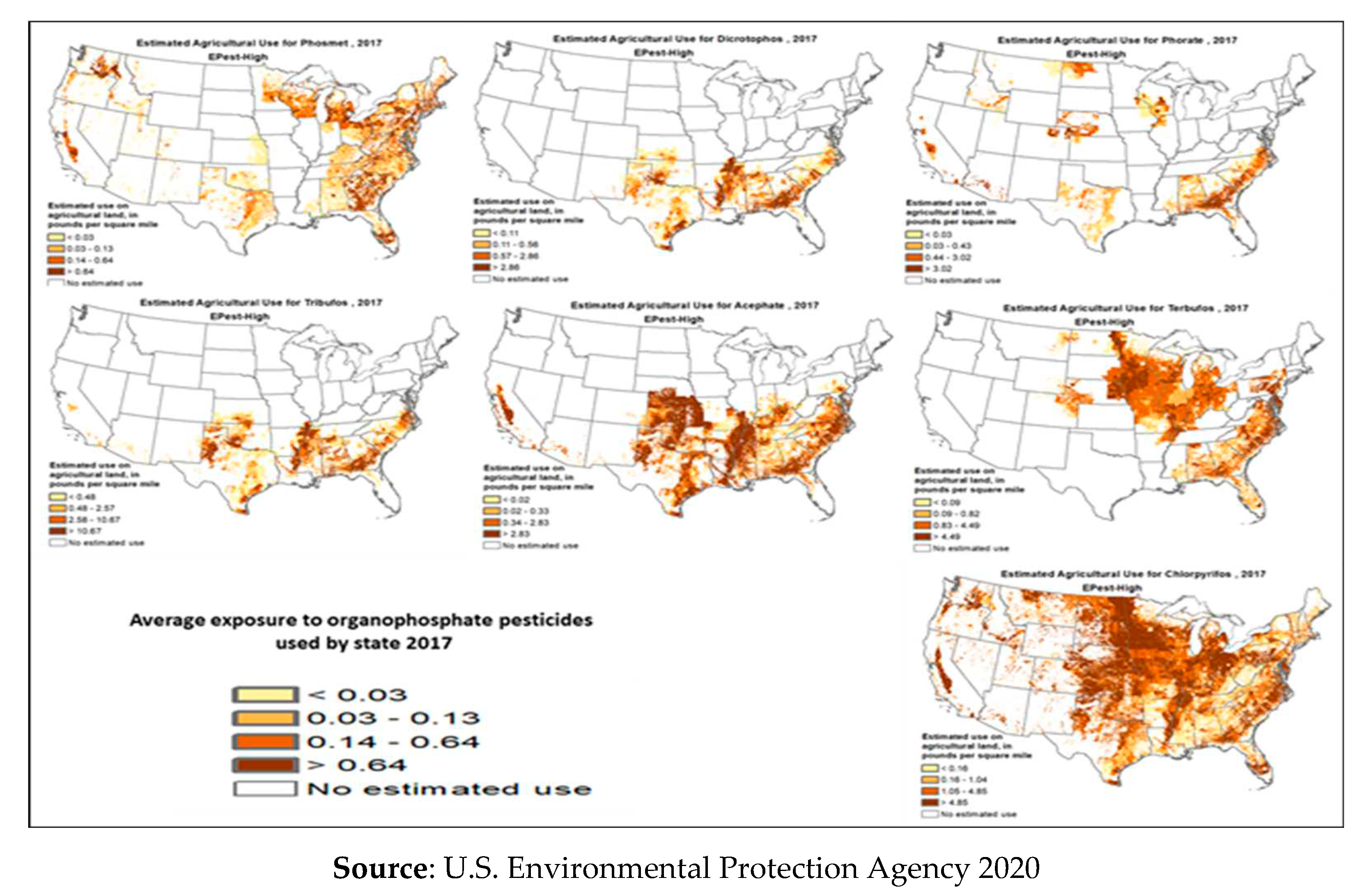
The annual agricultural pesticide database at the U.S. Geological Survey (USGS) are displayed in (Table 2 and Table 3) to specify the amount of data on pesticide consumption. Pesticide use reporting data both USEPA and the USDA National Agricultural Statistics Service (NASS) collect annual data on the sale and use of pesticides at the state level Figure 3) [39,40].
Figure 3.
The average exposure to organophosphate pesticides used by the state in 2020.
2.2.3. Gridded population data.
Population data were obtained from the 2021 NASA’s SEDAC (Socioeconomic Data and Applications Center) project at Columbia University database, which aggregates census block data and residential/household information into latitude-longitude grids at a 30 arc-second resolution [41]. The SEDAC data was selected to avoid irregular unit shapes of census units and to achieve high-resolution exposure information that also could be up-scaled to census units [29]. SEDAC enables this study to work outside of census blocks and buffer population over land cover data. The data frame projection was set to the total population using GCS_WGS_1984, and datum D_WGS_84 (www.earthdata.nasa.gov).
2.3. The Methodology.
The methodology for the current study was modeled from various studies: [27,28,29,30,31]. The methodology has assumed that all croplands in Macon County are using pesticides and that all public and private farms adhere to restrictions concerning the standard quantities of pesticides used. Furthermore, pesticides will drift off-target evenly taking the primary drivers (wind, followed by humidity, and nozzle technology) into account. Pesticide weight and specific drift potential for the chemical were accounted for.
Supervised classification with the maximum likelihood method has been performed to classify different LULC types based on pixel training spectral signatures for each class, we divided the map into four categories. The classified cropland uses included all crops in Macon County using ArcGIS 10.8.2. The MLC method takes into account the variance of each signature and assumes that the probability of class membership is the same for all classes. When comparing a pixel to a signature, this variance is crucial. The following is the maximum likelihood equation for each of the classes:
Where X is the measurement vector of the pixel, Mc is the mean vector of the class, T is the matrix transpose function, D is the weighted distance, 1n is a natural logarithm function, COV is the covariance matrix for a certain class. According to Wan, 2015, in the current study, agriculture pesticide drifts exposure linked to the Macon population grid level is calculated using a buffer zone-based exposure drift model.
Where Ci represents the number of pixels for the Ith crop, Wi represents the average pesticide usage for the Ith crop, Pt represents the total amount of pesticide used for the entire county, Pci represents the total pesticide usage for the crop I within the county.
To convert the population raster grid to points, to calculate the population volume and density; we created for each cell of the input raster dataset, a point positioned at the centers of cells that they represent. Using raster to point, centroids were created on each cell creating a point at the cell center with the grid code that equates to the total population value of the cell.
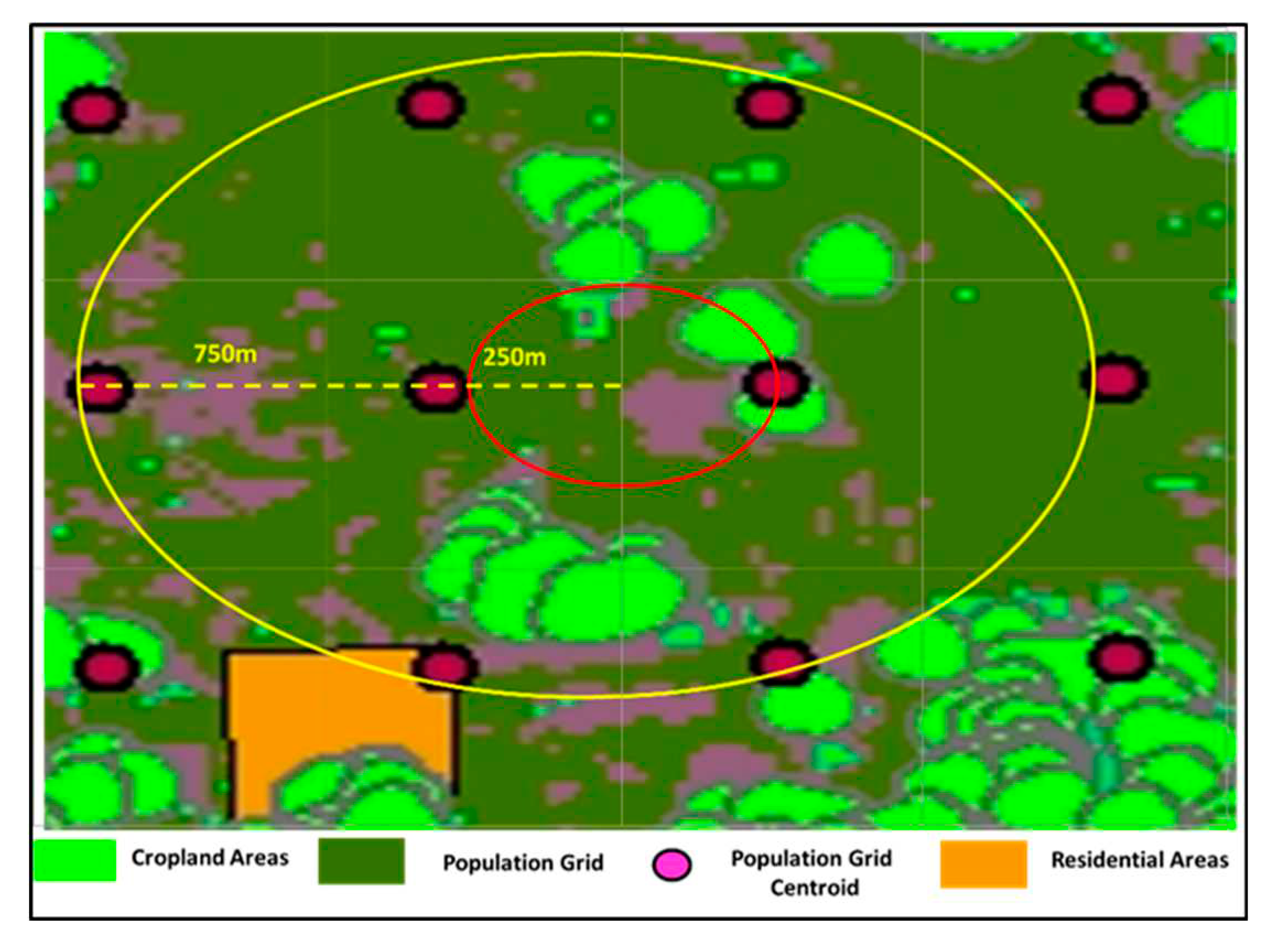
As many GIS-based exposure drift studies rely on pesticides spreading within a particular buffer zone to measure exposure, the accuracy of the buffer zone becomes vital. Establishing a specific buffer zone is complex due to various considerations such as climate conditions, chemical compositions of pesticides, and application techniques [31]. We converted a raster dataset obtained from NASA’s SEDAC database to point to features, for each cell of the input raster dataset, centroids were created on each cell creating a point at the cell center with the grid code that equates to the total population value of the cell. From this centroid, a 400-m buffer zone was created off the pivotal point of each cell.
A buffer zone has been created for each population grid, measured all pixels in the buffer that were classified as cropland areas, and summarized the estimated pesticide usage. To calculate the buffer zone, a distance of 750 m was used as a mean pesticide drifting distance, and this distance was added to the length of population grids, which is approximately 1000 m divided into four sides:
Where Bz is the buffer zone, Pd is the mean pesticides drift, and Pg is the population grid. It is noteworthy that this equation agrees with [25,26,27,28,29,30,31], [42,43,44] studies. A proximity measure, for example, determines that an individual or area unit is exposed to agricultural pesticide drift if its location is within a certain distance of agricultural land; an acreage measure assumes that exposure level is proportional to the total acreage of agricultural lands surrounding the residential location.
From this centroid, a 437.5-m buffer was created off the pivotal point of each cell. Utilizing the geodesic method which maintained an oval shape and was converted into arc seconds. All the buffer zones with a centroid located within Macon County were selected. Zonal statistics were run using the 437.5-m circle to calculate the total cropland pixels for each circle as shown in (Figure 4). The pesticide-weighted exposure has been calculated by creating a buffer zone for each residential area and calculating all pixels that were classified crops within the specified buffer zone, and finally, summarizing the amount of estimated pesticide use.
Figure 4.
Buffer zone-based pesticide exposure and population grid modeling.
3. Results and discussion
Despite the study’s limitations, the study’s assumptions were mostly reasonable and appropriate for achieving spatial accuracy at the county level. Our study assumed that all crops in Macon County used permitted pesticides in the amounts specified. Our research also hypothesized that pesticides would drift evenly away from their intended targets, depending on the type of application used (ground, orchard, or aerial); thus, standard distances for each application were used.
Due to a lack of accurate pesticide data in Macon County; our study developed a method that maximizes the benefits of GIS applications and remote sensing tools in extracting land use land cover data, population distribution data, and pesticide use data at the county level to estimate agricultural pesticide exposure drift.
This study defined the main categories of land use land cover, and utilized the Normalized Difference Vegetation Index (NDVI) as an indicator to calculate the MLC using a data reduction technique enhanced by resizing the spatial resolution of Landsat (30m) with the Sentinel-2 satellite image (10m). Our study maximized the benefits of the MLC method by obtaining accurate data (30m) for Macon County as shown in (Figure 5) and in a 10-m spatial resolution for the cropland, water bodies, vegetation, forests, and residential areas of Macon County as shown in (Figure 6 and Figure 7).
(Figure 6 and Figure 7) depict the classes of land cover categories for the main cities in Macon County with 10 m spatial resolution. Notably, all categories exhibited a great match with ground reality after applying the accuracy assessment, with only a few exceptions for some grid points in the southern margins of Macon County. In Macon County, agriculture constitutes the predominant type of land use. Due to its flat topography and rich soil, Macon County is perfect for mono-cropping, which is the method used for growing cotton and corn.
The water bodies contributed 2.5% of the total Macon County area, and the residential area explains 6.6% of the maximum likelihood classification results. Where the percentage of croplands was about 15.5%, and finally, the forests and vegetation areas represented the majority of Macon County, where they represented about 76%. This percentage can be expected, given the agricultural nature of Macon County. In particular, they often receive larger amounts of pesticides than other urban counties, and accordingly, they are more sensitive to even small amounts of seasonal pesticide applications. We relied on the croplands shown in (Figure 6 and Figure 7) to estimate the quantities of pesticide usage in kilograms.
Figure 8 shows the population-gridded data that has been derived and employed to fill the gap in obtaining accurate data, particularly regarding the volume and distribution of the population in Macon County. The spatial pattern of population density is mostly homogeneous to the pesticide usage display, with the population in the central and western regions and Tuskegee experiencing no exposure.
This study found that 62% of the population of rural areas in the eastern and southern parts are exposed to the drift of pesticides within buffer zone 437.5 m, and this percentage increases and reaches 74% when applying the 380-m buffer zone range, as shown in (Figure 9).
In detail, the results further indicate that 6.6 percent of about 1000 residents of Macon County’s total population are considered potentially severely exposed, and the affected population resides primarily in rural areas. The results indicate that 23 percent of about 3340 residents of Macon County’s total rural population are considered potentially medium- to high exposure. While 38% of about 5,500 residents in a suburban area are considered to have potentially low to medium exposure.
Pesticide exposure is almost non-existent in the county’s south and east-central regions (which are primarily covered by forest). It can be observed from (Figure 10 and Figure 11) that the pesticides used are in close accordance with crop distributions and local geographic characteristics. Macon County is the least populated in the eastern part of Alabama, where more croplands and forests and fewer residential areas occur, with about 19532 persons in 2020.
Higher pesticide exposure occurs in the southern and eastern parts of Macon County, whereas the northern part of the county is located close to a main urban area and has considerably less exposure. Residents in Tuskegee City, the county seat and first most populated area, showed very weak exposure to pesticides, as shown in (Figure 11).
Figure 11. Illustrates the average of pesticide exposure categories over Macon County based on Wan’s (2015) proposed exposure model, which has been upscaled from population grid exposure data. The population in the middle and northwestern provinces, as well as those in the capital Tuskegee, Notasulga, Shorter, and Franklin, were exposed to moderate-to-weak drift. Accordingly, the current study could estimate the total residential exposure to drift and identify areas of high exposure.
Figure 11. Also explains that the southern and eastern boundaries of Tuskegee town have had agricultural areas, and thus high exposure to pesticides, but at the same time have exceeded the maximum limit of the buffer zone, and thus the risk of exposure to pesticide drift for Tuskegee residents is very weak.
Figure 12. Depicts the pattern of Organophosphate Pesticide exposure drift in Macon County, which was derived from exposure information from population grids and based on Table 2 data. It can be concluded that the area under the administration of Macon County reached 38,963 acres, which represents 1.20% of Alabama. It is also clear that acres of harvested cropland reached 26,305 acres, which represents 1.19% of Alabama, the square miles of harvested cropland in Macon County in 2021 reached 41 SQ_MI_HC.
It can be observed that the log of the concentration of pesticide uses across harvested cropland for EPest-high estimates for Macon County is 2.3 kg For EPest-high estimates, the pesticide concentration across harvested cropland was 199.61 pounds per square mile. The sum of the EPest-high estimates for pesticides is 3721.66 kg. The sum of the EPest-high estimates for pesticides in pounds (lbs) reached 8204.72. The urban agricultural interface of the county were with high levels of exposure drift, those with average exposure greater than 25 kg/ha were concentrated. Urban areas had substantially lower exposure risk levels lower than 10 kg/ha.
Figure 12 also illustrates pesticide usage in Macon County in 2020. As shown in the figure, high-usage areas were mostly concentrated in the county’s southern and central regions, which corresponded to the main cropland concentration areas. Albeit with their coverage of more than 25.000 kg of agricultural pesticide usage, the characterization of Tuskegee, Notasulga, Franklin, Woodland, and Shorter in the high-usage pesticide category is not well understood from a practical perspective.
This is mainly due to the uneven geographical distribution of pesticide information over time and space, particularly at more residential sites, and also attributed to high population density, and the long distance of cropland away from those cities.
4. Conclusion
This study proposed a remote sensing and GIS approach to generate helpful information about Macon population exposure to pesticide drift on a county level. This study illustrated how to generate practical indicators of pesticide exposure drift using the suggested method based on the usage of organophosphate pesticides. Albeit with the current study limitations, it provided a real and accurate assessment of pesticide exposure drift. This methodology should serve as a framework to inform more detailed studies that combine the trends of drift. This study concluded that an essential limitation in pesticide drift exposure is that it is difficult to determine the area of the buffer zone. Also, it may be attributed to local factors related to the area of the study area and the extent to which residential areas are close to or far from agricultural areas.
It can be concluded that the overlay of population grid data, and pesticide usage data with LULC was remarkably useful for identifying residential areas in Macon County with potentially high risks of exposure to pesticide drift. In this study, remote sensing and GIS tools provided an accurate spatial analysis of potential pesticide exposure drift, indicating that rural populations in Macon County are disproportionally exposed to pesticide drift. Also, allow researchers to examine high-exposure areas more closely.
Our study demonstrated that Macon County is a mix of rural and urban residents, making it well suited to determine how many of the county’s residents are at high exposure and to examine the spatial pattern of potential population grid exposure to pesticide drift. This study also concluded that rural residents have a higher pesticide exposure risk than urban residents, which poses a hazard for farmers and applicators utilizing pesticides in their practices. We concluded that the potential exposure to pesticide drift was concentrated in rural areas, with low population densities in Macon County’s central and southern regions. The potential exposure to pesticide drift is further reduced away from rural areas, especially near major cities in the center and west.
The current study accords with Dappen et al., (2008) and Wan (2015) that rural areas are at a higher pesticide exposure drift, indicating the necessity for a more accurate examination of rural areas. Future research should focus on isolating rural areas and estimating pesticide exposure drift based on the actual number of rural populations. Estimating the exposure drift at the county and state levels is unreliable when non-rural areas are considered, and it reduces the potential impact of exposure outcomes. The lack of a suitable model for estimating pesticide drift in Alabama motivated the work team to develop previous research attempts and a model that is compatible with the residential environment and weather conditions of Macon County, and previous research backs it up.
This study provided an accurate evaluation of pesticide drift; it could be the first study of the Southeastern Counties that can highlight potential geographic areas of high exposure drift. Our study also demonstrated the effectiveness of utilizing remote sensing and GIS techniques to estimate the agricultural pesticide exposure drift, notably in regions that do not have accurate data on the number of pesticides used, population numbers, or croplands.
Author Contributions
All authors listed have made a substantial, direct, and intellectual contribution to the work and approved it for publication.
Funding
This work is funded by the 1890 Capacity Building Grants Program (CBG) [Grant No. 2020-38821-31084 /project accession No. 1021820] from the USDA National Institute of Food and Agriculture.
Data Availability Statement
The datasets generated during and/or analyzed during this study are available from the corresponding author on reasonable request.
Acknowledgments
The authors would like to thank USDA National Institute of Food and Agriculture for Support and financing.
Conflicts of Interest
The authors declare no conflict of interest. The funders had no role in the design of the study; in the collection, analyses, or interpretation of data; in the writing of the manuscript; or in the decision to publish the results.
References
- Benbrook, Charles, M. 2019. “How did the US EPA and IARC reach Diametrically Opposed Conclusions on the Genotoxicity of Glyphosate-based Herbicides?” Environmental Sciences Europe 31, no. 1: 2.
- Burchfield, Shelbie, L., Denise, C. Bailey, Callie, E. Todt, Rachel, D. Denney, Rekek Negga, and Vanessa, A. Fitsanakis. “Acute exposure to a glyphosate-containing herbicide formulation inhibits Complex II and increases hydrogen peroxide in the model organism Caenorhabditis elegans.” Environmental Toxicology and Pharmacology 66 (2019): 36-42.
- Centner, Terence, J., Levi Russell, and Matthew Mays. “Viewing evidence of harm accompanying uses of glyphosate-based herbicides under US legal requirements.” Science of the Total Environment 648 (2019): 609-617.
- Worldatlas (2022) https://www.worldatlas.com/articles/toppesticide-consuming-countries-of-the-world.html.
- Sharma, A., Kumar, V., Shahzad, B. et al. Worldwide pesticide usage and its impacts on ecosystem. SN Appl. Sci. 1, 1446 (2019). [CrossRef]
- Wang, Magnus, and Dirk Rautmann. 2008. “A Simple Probabilistic Estimation of Spray Drift— Factors Determining Spray Drift and Development of a Model.” Environmental Toxicology and Chemistry 27, no. 12: 2617-2626.
- Boffetta, Paolo, Hans-Olov Adami, Colin Berry, and Jack, S. Mandel. 2013. “Atrazine and Cancer: A Review of the Epidemiologic Evidence.” European Journal of Cancer Prevention 22, no. 2: 169-180.
- Chen, Mei, Chi-Hsuan Chang, Lin Tao, and Chensheng Lu. 2015. “Residential exposure to pesticide during childhood and childhood cancers: A meta-analysis.” Pediatrics 136, no. 4: 719-729.
- VoPham, Trang, Maria, M. Brooks, Jian-Min Yuan, Evelyn, O. Talbott, Darren Ruddell, Jaime, E. Hart, Chung-Chou, H. Chang, and Joel, L. Weissfeld. 2015. “Pesticide Exposure and Hepatocellular Carcinoma Risk: A Case-Control Study using a Geographic Information System (GIS) to link SEER-Medicare and California Pesticide Data.” Environmental Research 143: 68-82.
- Curl, C.L., Spivak, M., Phinney, R. et al. Synthetic Pesticides and Health in Vulnerable Populations: Agricultural Workers. Curr Envir Health Rpt 7, 13–29 (2020). [CrossRef]
- Koureas, M., Tsakalof, A., Tsatsakis, A., Hadjichristodoulou, C., 2012. A systematic review of biomonitoring studies to determine the association between exposure to organophosphorus and pyrethroid insecticides and human health outcomes. Toxico. Lett. 210, 155–168.
- Sanchez-Santed, F., Colomina, M.T., Hern’ andez, E.H., 2016. Organophosphate pesticide exposure and neurodegeneration. Cortex 74, 417–426.
- Lacasana, ˜ M., Lopez-Flores, ´ I., Rodríguez-Barranco, M., Aguilar-Garduno, C., BlancoMunoz, J., P.´erez-M.´ endez, O., Gamboa, R., Bassol, S., Cebrian, M.E., 2010. Association between organophosphate pesticides exposure and thyroid hormones in floriculture workers. Toxicol. Appl. Parmaco. 243, 19-26.
- Yan, Holly. “The EPA Says Glyphosate, the Main Ingredient in Roundup, Doesn’t Cause Cancer. Others aren’t so sure.” May 3, 2019. CNN.com. https://www.cnn.com/2019/05/01/health/epa-says-glyphosate-is-safe/index.html.
- Blair, Aaron, Beate Ritz, Catharina Wesseling, Laura Beane Freeman. 2014. “Pesticides and Human Health.” Occupational Environmental Medicine 0: No 0. 1-2.
- Wesseling C, McConnell R, Partanen, T., Hogstedt, C. Agricultural pesticide use in developing countries: Health effects and research needs. Int J Health Serv. 1997;27:273–308. [CrossRef]
- Allpress, J.L., Curry, R.J., Hanchette, C.L., Phillips, M.J., & Wilcosky, T.C. (2008). A GIS-based method for household recruitment in a prospective pesticide exposure study. International Journal of Health Geographics, 7(1), 18.
- Shirangi, A., Nieuwenhuijsen, M., Vienneau, D., & Holman, C.J. (2011). Living near agricultural pesticide applications and the risk of adverse reproductive outcomes: A review of the literature. Pediatric and Perinatal Epidemiology, 25(2),172e191.
- Figueiredo DM, Krop EJM, Duyzer J, Gerritsen-Ebben RM, Gooijer YM, Holterman HJ, Huss A, Jacobs CMJ, Kivits CM, Kruijne R, Mol HJGJ, Oerlemans A, Sauer PJJ, Scheepers PTJ, van de Zande JC, van den Berg E, Wenneker M, Vermeulen RCH. Pesticide Exposure of Residents Living Close to Agricultural Fields in the Netherlands: Protocol for an Observational Study. JMIR Res Protoc. 2021 Apr 28;10(4):e27883. [CrossRef]
- Maxwell, Susan, K., Matthew Airola, and John, R. Nuckols. 2010. “Using Landsat Satellite Data to Support Pesticide Exposure Assessment in California.” International Journal of Health Geographics 9, no. 1: 46.
- Maxwell, Susan, K., Jaymie, R. Meliker, and Pierre Goovaerts. 2010. “Use of Land Surface Remotely Sensed Satellite and Airborne Data for Environmental Exposure Assessment in Cancer Research.” Journal of Exposure Science and Environmental Epidemiology 20, no. 2: 176.
- Marusek JC, Cockburn MG, Mills PK, Ritz BR. Control selection and pesticide exposure assessment via GIS in prostate cancer studies. Am J Prev Med [Internet]. 2006; 30(2 SUPPL.):S109–16.
- Ritz, B., Costello, S. Geographic model and biomarker-derived measures of pesticide exposure and Parkinson’s disease. In: Mehlman MA and Soffritti M and Landrigan P and Bingham E and Belpoggi F, editor. Living in a chemical world: Framing the future in light of the past. 2006. p. 378–87.
- Nuckols JR, Gunier RB, Riggs P, Miller R, Reynolds, P., Ward MH. Linkage of the California Pesticide Use Reporting Database with spatial land use data for exposure assessment. Environ Health Perspect. 2007; 115(5):684–9.
- Ward, Mary, H., Jay Lubin, James Giglierano, Joanne, S. Colt, Calvin Wolter, Nural Bekiroglu, David Camann, Patricia Hartge, and John, R. Nuckols. 2006. “Proximity to Crops and Residential Exposure to Agricultural Herbicides in Iowa.” Environmental Health Perspectives 114, no. 6: 893.
- Teysseire R, Manangama G, Baldi I, Carles C, Brochard P, Bedos C; et al. (2020) Assessment of residential exposures to agricultural pesticides: A scoping review. PLoS ONE 15(4): e0232258. [CrossRef]
- Dappen, P., Merchant, J., Ratcliffe, I., & Robbins, C. (2007). Delineation of 2005 land use patterns for the state of Nebraska. Lincoln, NE: Center for Advanced Land Management Information Technologies, School of Natural Resources, University of Nebraska-Lincoln.
- Wang, Anthony, Sadie Costello, Myles Cockburn, Xinbo Zhang, Jeff Bronstein, and Beate Ritz. 2011. “Parkinson’s Disease Risk from Ambient Exposure to Pesticides.” European Journal of Epidemiology 26, no. 7: 547-555.
- Wan, Neng. 2015. “Pesticides Exposure Modeling Based on GIS and Remote Sensing Land Use Data.” Applied Geography 56: 99-106.
- Brouwer, Maartje, Hans Kromhout, Roel Vermeulen, Jan Duyzer, Henk Kramer, Gerard Hazeu, Geert De Snoo, and Anke Huss. 2018. “Assessment of residential environmental exposure to pesticides from agricultural fields in the Netherlands.” Journal of Exposure Science and Environmental Epidemiology 28, no. 2: 173.
- Anna Myers, 2019. “Modeling Exposure to Pesticide Drift in Madison County, Illinois.” A Thesis Submitted in Partial Fulfillment of the Requirements for the Degree of Master of Science in the Field of Geography. Southern Illinois University Edwardsville, P.76.
- USGS (United States Geological Survey). 2019. Pesticide use maps. https://water.usgs.gov/nawqa/pnsp/usage/maps/show_map.php?year=2015%26map=GLYPHOSATE%26hilo=L.
- Wieben, C.M., 2021, Estimated annual agricultural pesticide use by major crop or crop group for states of the conterminous United States, 1992-2019 (including preliminary estimates for 2018-19): U.S. Geological Survey data release. [CrossRef]
- USA Facts. 2020. Who is the American farmer? https://usafacts.org/articles/farmer-demographics/.
- ADECA, “Memorandum of Understanding between the State of Alabama Department of Finance and ADECA,” 2020. https://governor.alabama.gov/assets/2020/07/Finance-ADECA-MOU-ABCfor-Students.pdf (accessed Apr. 18, 2023).
- USDA (United States Department of Agriculture). 2021. Pesticide use and markets. https://www.ers.usda.gov/topics/farm-practices-management/chemical-inputs/pesticide-use-markets.aspx.
- Farm Service Agency, U.S. Department of Agriculture. https://www.fsa.usda.gov/online-services/fsa-online-data-resources/index(Last seen, 02/22/2022).
- Pesticide National Synthesis Project, National Water-Quality Assessment (NAWQA) Project. https://water.usgs.gov/nawqa/pnsp/usage/maps/compound_listing.php (Last seen, 02/25/2022).
- CropScape-Cropland Data Layer project, National Agricultural Statistics Service (NASS)/USDA https://nassgeodata.gmu.edu/CropScape/ (Last seen, 02/01/2023).
- U.S. Environmental Protection Agency. Refined Ecological Risk Assessment for Atrazine. By Frank, T. Farruggia, Colleen, M. Rossmeisl, James, A. Hetrick, Melanie Biscoe, Rosanna Louie-Juzwiak, and Dana Spatz, Washington, D.C. April 12, 2019. https://www.regulations.gov/document?D=EPA-HQ-OPP-2013-0266-0343.
- Socioeconomic Data and Applications Center (SEDAC), Population Estimation Service (PES). https://sedac.ciesin.columbia.edu/data/collection/gpw-v4/population-estimation-service.
- Atay, Eren, and Peter Ayebare. 2017. “Determination of Buffer-Zones Using Agricultural Information System.” TEM Journal 6, no. 2: 363.
- Bell, Erin, M., Irva Hertz-Picciotto, and James, J. Beaumont. 2001. “A Case-Control Study of pesticides and fetal death due to congenital anomalies.” Epidemiology 12, no. 2: 148-156.
- Bellaloui, Nacer, Krishna, N. Reddy, Robert, M. Zablotowicz, and Alemu Mengistu. 2006. “Simulated glyphosate drift influences nitrate assimilation and nitrogen fixation in non-glyphosate-resistant soybean.” Journal of Agricultural and Food Chemistry 54, no. 9: 3357-3364.
Figure 1.
The location of Macon County, Alabama.
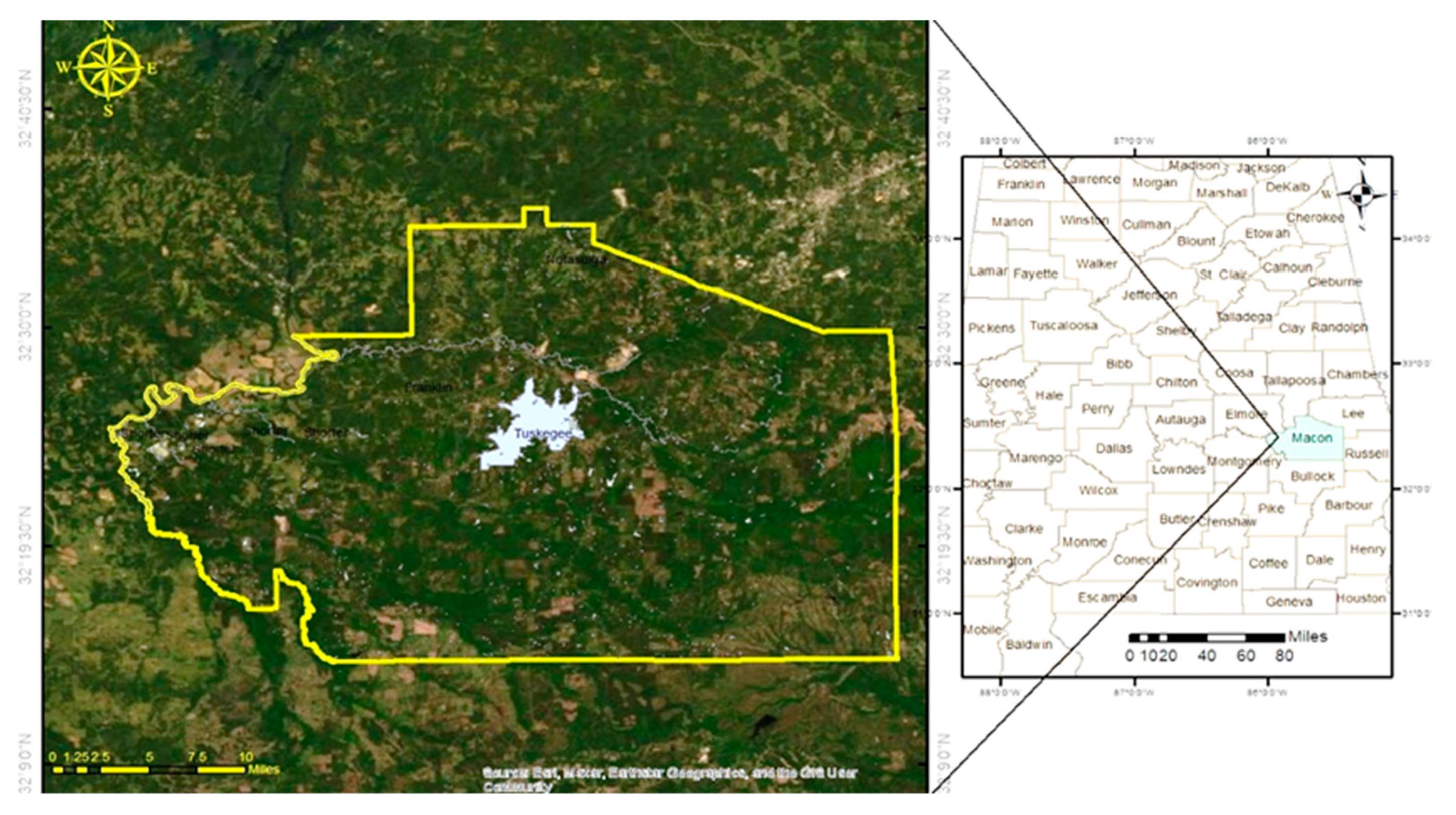
Figure 2.
The study dataset and methodology.
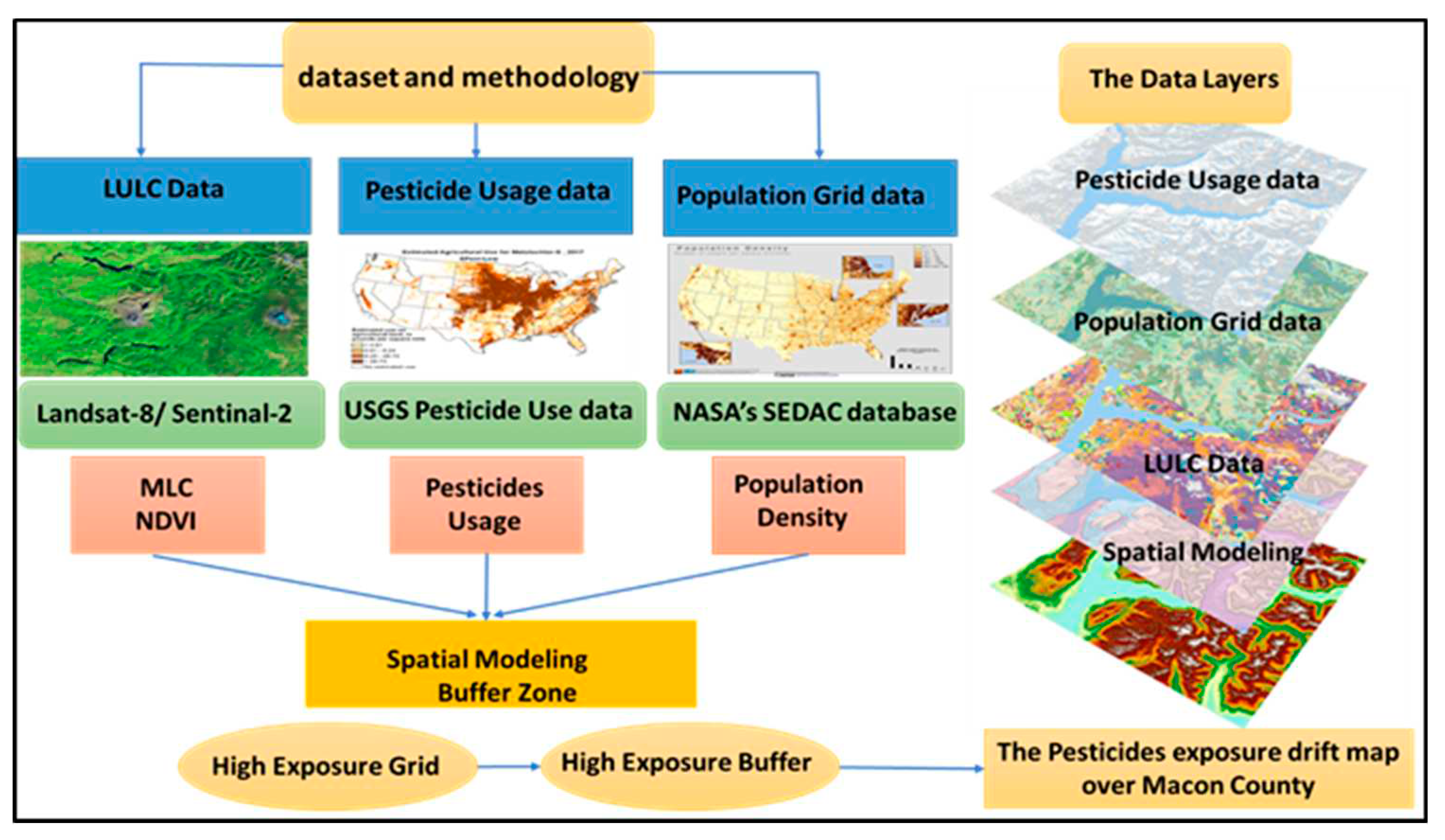
Figure 3.
The cropland layer data over Macon County, 2021

Figure 5.
Supervised classification of Macon County 30 m.
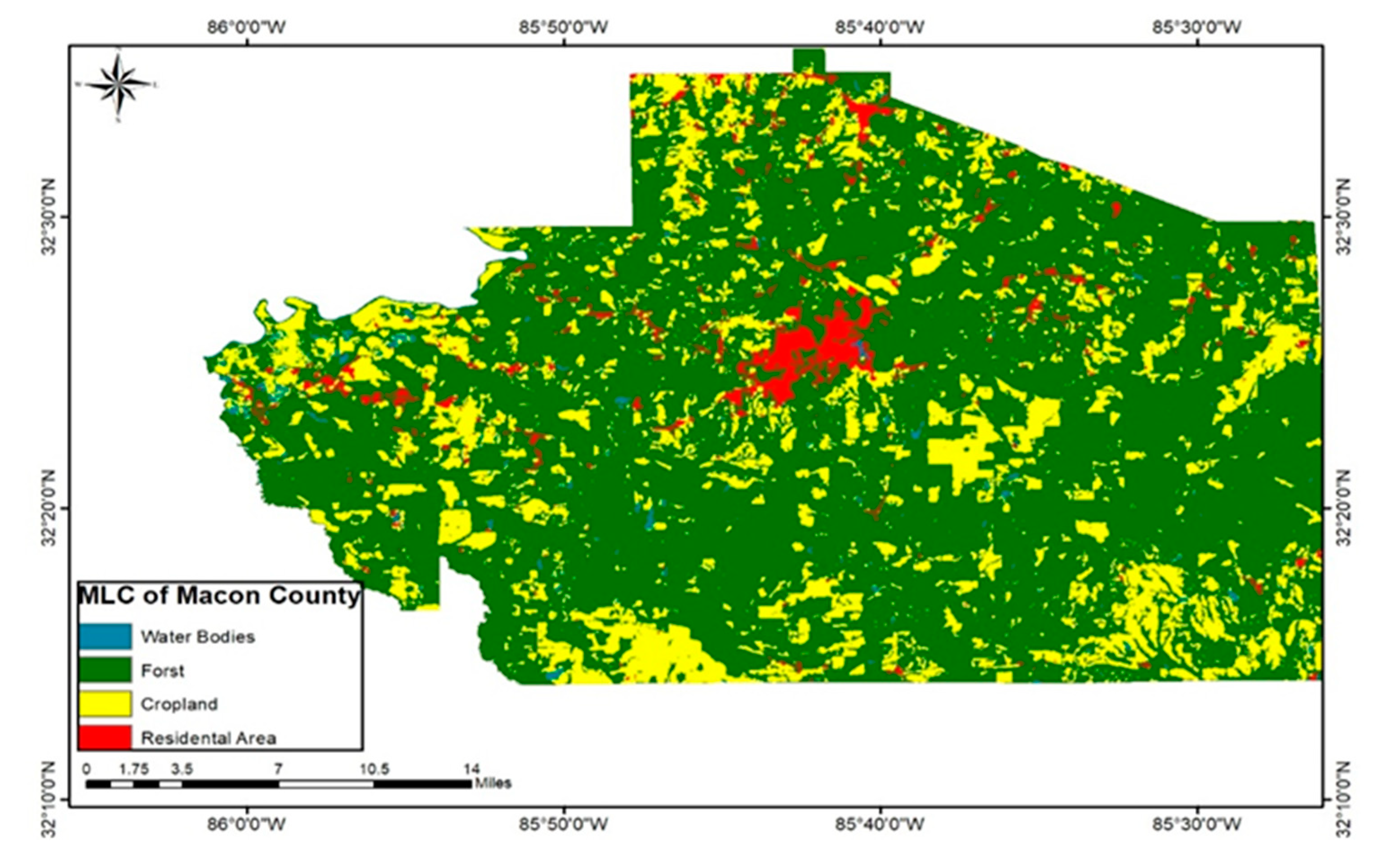
Figure 6.
Maximum Likelihood Classification of Tuskegee on the right and Franklin in the lift 10 m.
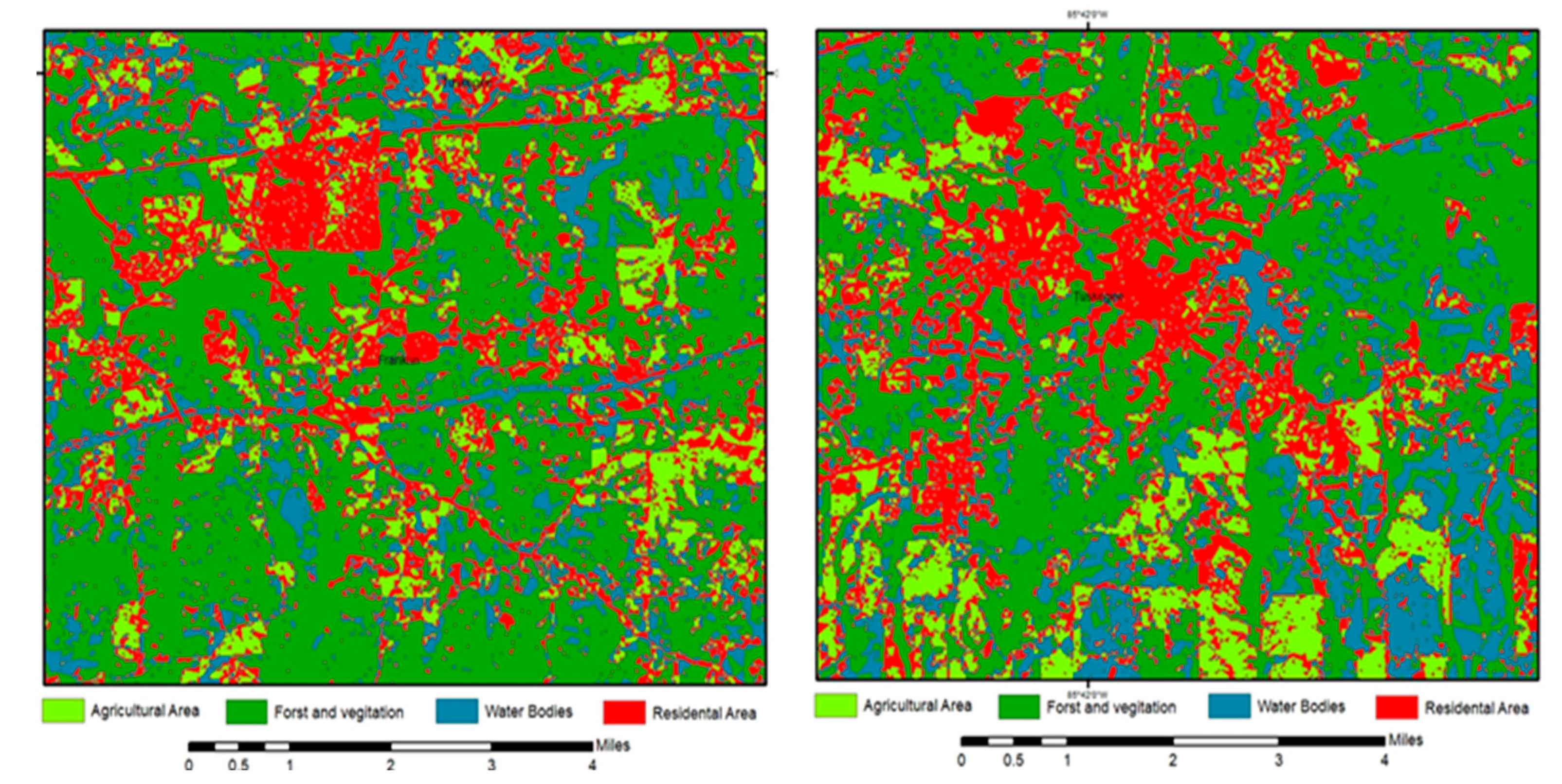
Figure 7.
Maximum Likelihood Classification of Notasulga on the right and Shorter on the left 10 m.
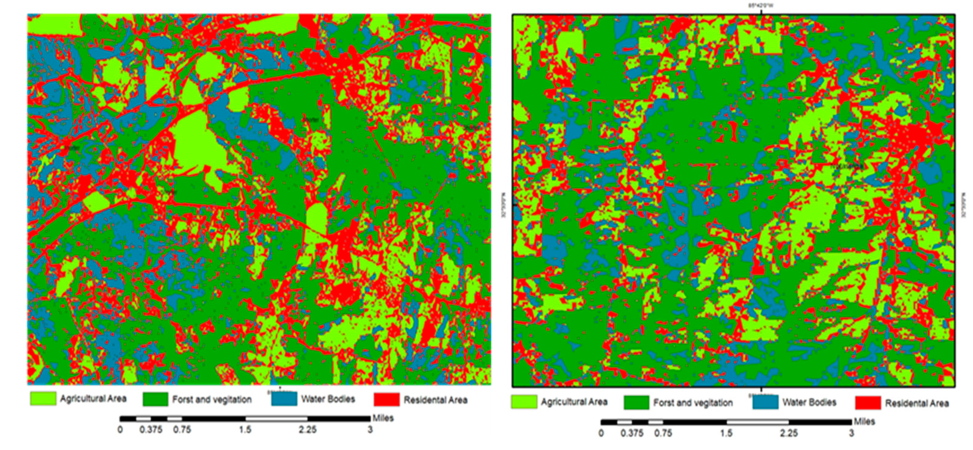
Figure 8.
Population Gridded data of Macon County.(Derived from NASA’s SEDAC Map Database)
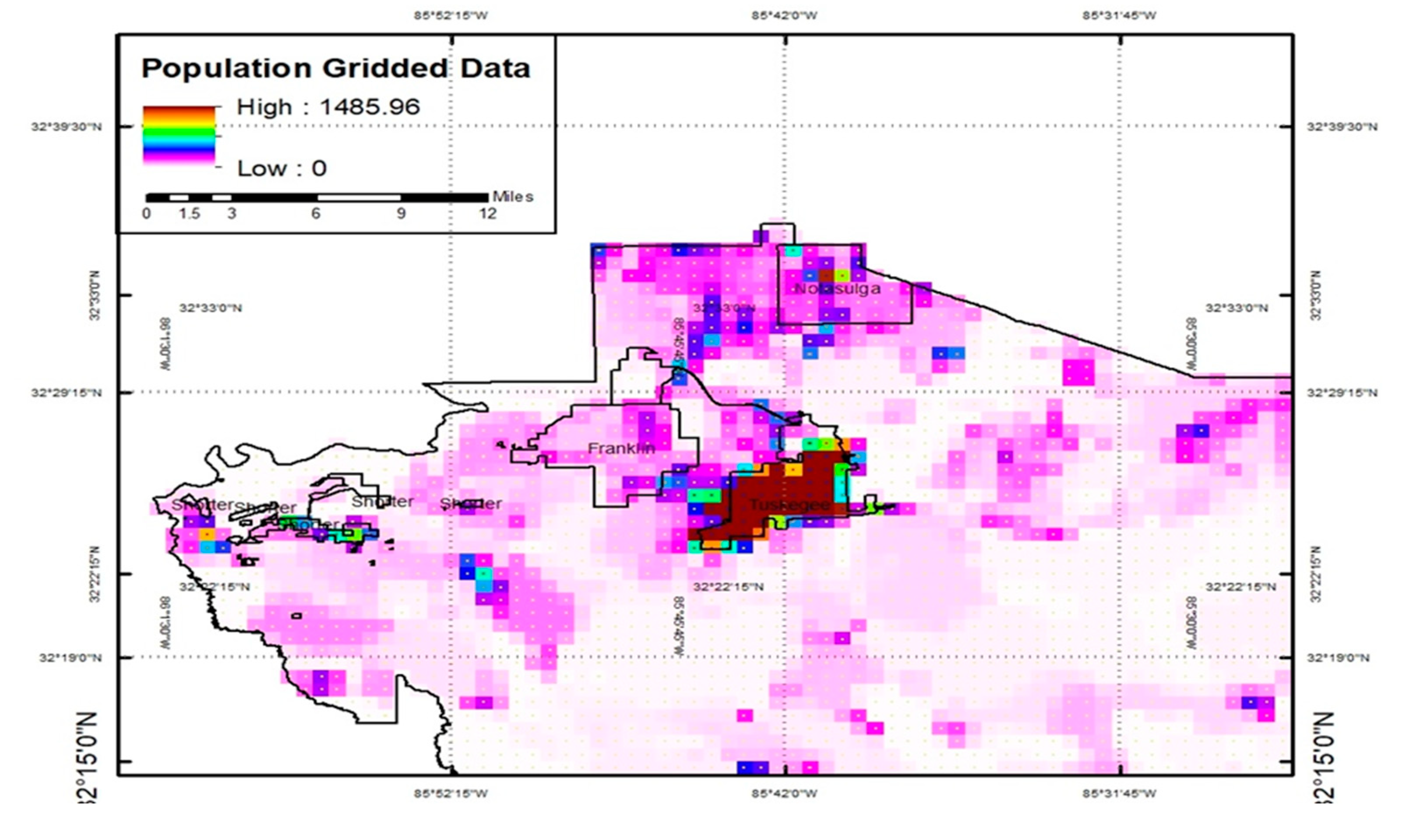
Figure 9.
Buffer zone-based pesticide exposure and population grid modeling.
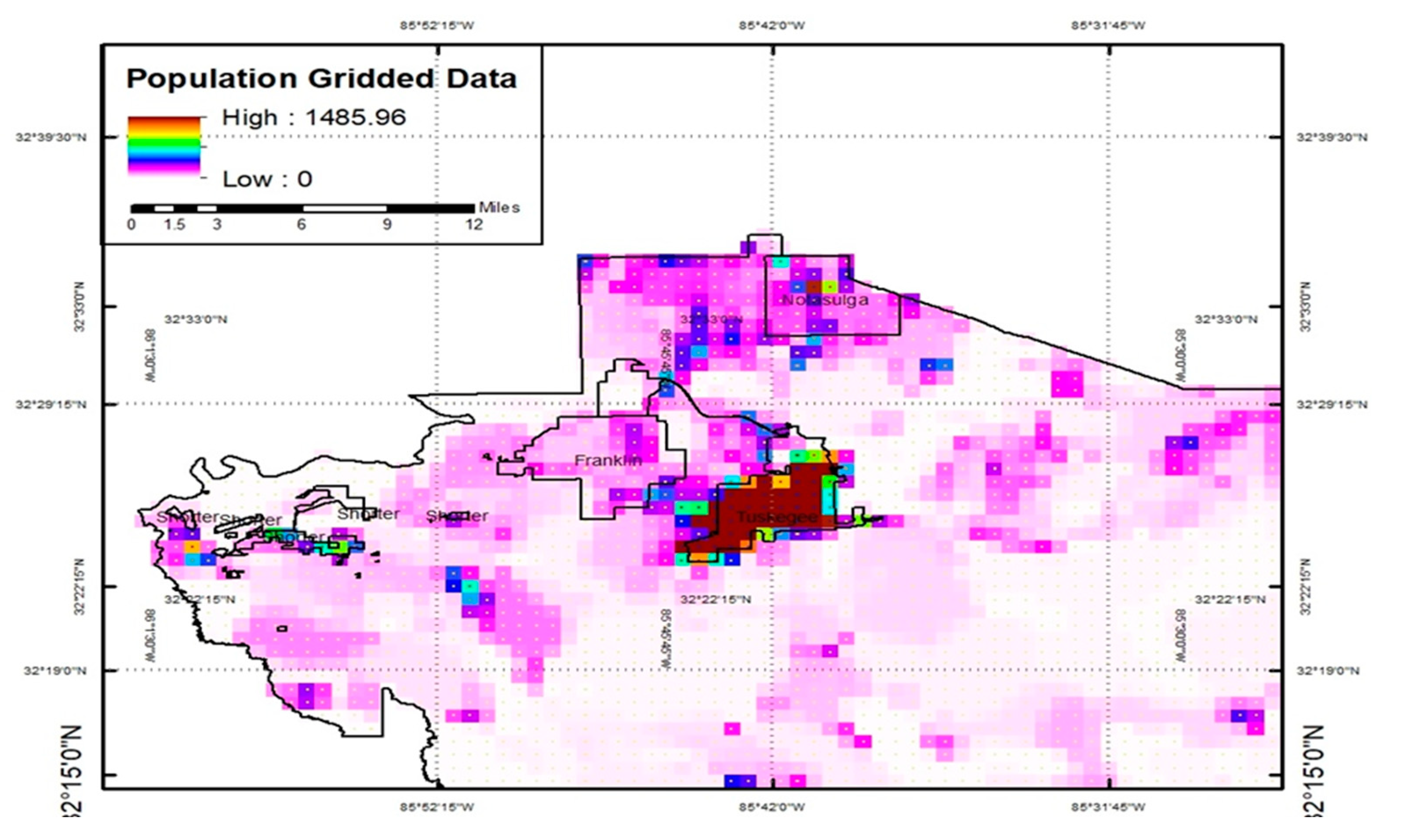
Figure 10.
The Potential high and low pesticide exposure drifts over Tuskegee.
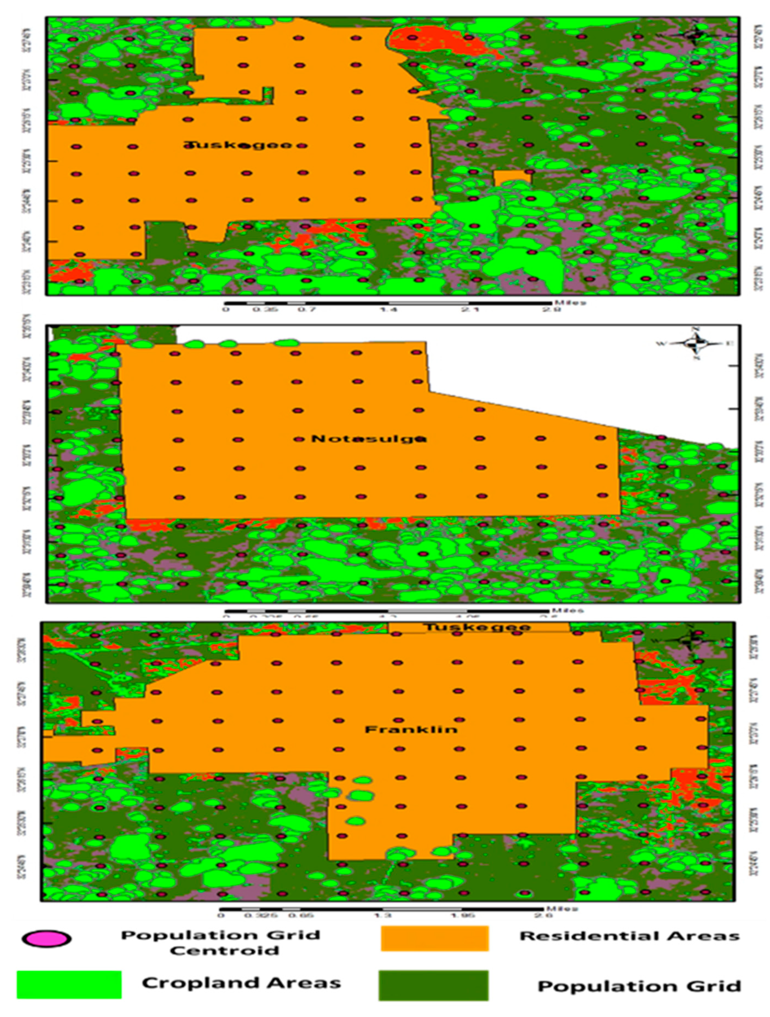
Figure 11.
The average of pesticide exposure categories over Macon County.
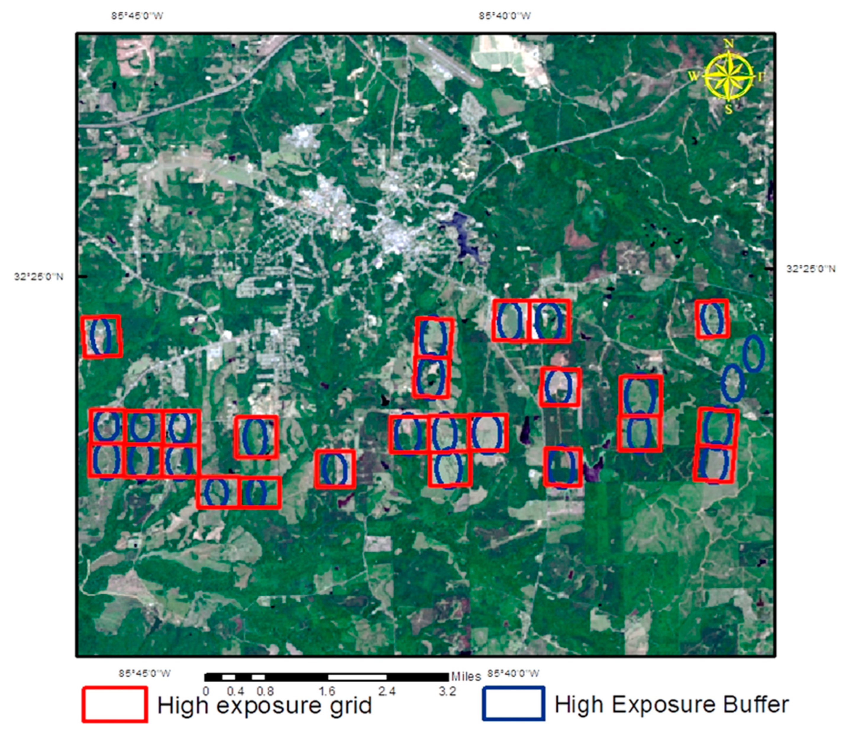
Figure 12.
The Pesticides usages over Macon County in (Kg) 2020.
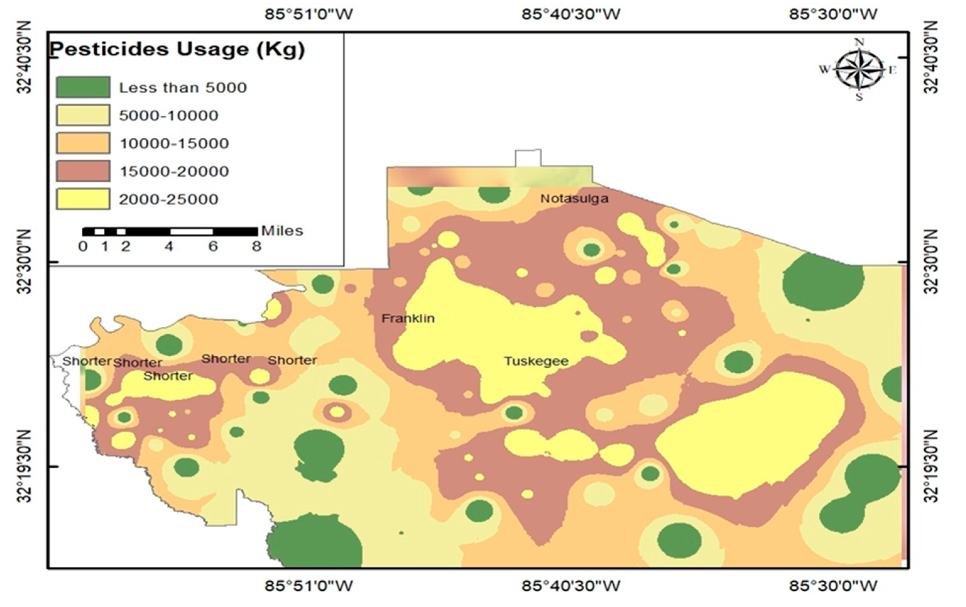
Table 2.
The pesticides usage in Macon County compared with Alabama, 2020.
| Items | Definition | Alabama | Macon | % |
|---|---|---|---|---|
| ATLAS_ACRE | Area of the administrative region in acres | 32,413,19 | 389,636 | 1.20 |
| ACRES_HC | Acres of harvested cropland | 2,205,766 | 26,305 | 1.19 |
| SQ_MI_HC | Square miles of harvested cropland | 50,647 | 41.00 | 0.1 |
| AGG_HI_KG | The sum of the EPest-high estimates for all 7 organophosphates, in kilograms (kg) | 235,141 | 3721.60 | 1.6 |
| AGG_HI_LB | The sum of the EPest-high estimates for all 7 organophosphates, in pounds (lbs) | 518,396 | 8204.72 | 1.5 |
| HI_LOG_RAT | The log of the concentration of organophosphate use across- harvested cropland for EPest-high estimates | 1,455.00 | 2.30 | 0.16 |
| HILBSQMIHC | The concentration of organophosphate unused cross harvested cropland, for EPest-high estimates, in pounds per square mile | 12.100.40 | 199.61 | 1.7 |
Source: U.S. Environmental Protection Agency 2020.
Table 3.
Organophosphate Pesticide Usage in Macon County, 2020.
| Pesticide name | Usage kg |
|---|---|
| ACEPHATE | 24.70 |
| CHLORPYR | 50.60 |
| DICROTOP | 94.30 |
| PHORATE | 410.50 |
| PHOSMET | 170.30 |
| TERBUFOS | 150.00 |
| TRIBUFOS | 2843.30 |
| Total | 3743.70 |
Source: U.S. Environmental Protection Agency 2020.
Disclaimer/Publisher’s Note: The statements, opinions and data contained in all publications are solely those of the individual author(s) and contributor(s) and not of MDPI and/or the editor(s). MDPI and/or the editor(s) disclaim responsibility for any injury to people or property resulting from any ideas, methods, instructions or products referred to in the content. |
© 2023 by the authors. Licensee MDPI, Basel, Switzerland. This article is an open access article distributed under the terms and conditions of the Creative Commons Attribution (CC BY) license (http://creativecommons.org/licenses/by/4.0/).
Copyright: This open access article is published under a Creative Commons CC BY 4.0 license, which permit the free download, distribution, and reuse, provided that the author and preprint are cited in any reuse.


