
Submitted:
10 April 2023
Posted:
10 April 2023
You are already at the latest version
Abstract
The use of plant growth-promoting bacteria can be one option for mitigating the impact of abiotic constraints on different cropping systems in the tropical semi-arid region. The aim of this study was to evaluate growth, leaf gas exchange and yield in maize inoculated with Bacillus aryabhattai, and subjected to water and salt stress. The experiment followed a randomised block design, in a split plot arrangement, with six repetitions. The plots comprised two levels of electrical conductivity for the irrigation water (ECw): 0.3 dS m-1 and 3.0 dS m-1; the subplots consisted of three irrigation depths (ID1: 50%, ID2: 75%, and ID3: 100% of the crop evapotranspiration (ETc)); while the sub-subplots included the presence or absence of Bacillus aryabhattai inoculant. A water deficit of 50% of the ETc resulted in the principal negative effects on growth, reducing the leaf area and stem diameter. The use of Bacillus aryabhattai mitigated salt stress and promoted better leaf gas exchange by increasing the CO2 assimilation rate, stomatal conductance, and internal CO2 concentration. However, irrigation with brackish water (3.0 dS m-1) reduced the instantaneous water use efficiency of the maize. Inoculation partially reduced the effects of abiotic stress due to morpho-physiological traits, and increased yield potential under water deficit with no salt stress.
Keywords:
Zea Mays
; abiotic stress
; microorganisms
; salinity
; water deficit
1. Introduction
Maize (Zea mays L.), with its origin in Central America, is of great economic importance, and is cultivated worldwide. In Brazil it is one of the main cereals produced (21,581.9 million hectares), with emphasis on food for human and animal consumption and bioenergy production [1,2,3,4]. The crop has gradually expanded into arid and semi-arid regions, where it helps to solve problems related to food security in places that have limited water resources [5,6].
The semi-arid region of Brazil is considered one of the largest semi-arid regions, with approximately 27 million inhabitants [7], where irrigation is an important tool for ensuring food security [8]. Characteristics of the region are high temperatures, high evapotranspiration, and a low rainfall rate [9,10]. Water shortages and high salt concentrations in the groundwater are problems that limit agricultural production in this region [8,11].
An excess of salts in the soil solution reduces water absorption by plants, and alters metabolic and morphological structures, causing a reduction in seed germination, growth, and productivity in agricultural crops [12,13,14]. Water and salt stress reduce the soil water potential, making the soil solution unavailable, or not readily available, for nutrient uptake by plants. These stresses have a negative effect on physiological processes, causing partial closure of the stomata, limiting the internal CO2 concentration, reducing the rates of photosynthesis and transpiration, and consequently water use efficiency and agricultural crop yields worldwide [15,16,17]. [18], evaluating the interaction between salt and water stress in the courgette, found a reduction in photosynthesis and transpiration. Similarly, [19] found a reduction in the productivity of peanuts under salt and water stress.
It should be noted that various strategies have been used in the scientific environment to mitigate salt and water stress. One alternative to mitigate the effects of such stress, and ensure production in agroecological systems, is the use of microbial inoculants formulated with plant growth-promoting bacteria (PGPB) [20,21,22]. These microorganisms can offer protection to plants against water deficit by maintaining moisture levels, and providing better root development and nutrient supply. Researchers are seeking to identify microorganisms, together with their action mechanisms, which are able to mitigate abiotic stress [23,24]. Various promising studies have found that inoculating maize with beneficial microorganisms results in greater productivity [25].
Given this promising scenario, the present study tested the hypothesis that the use of plant growth-promoting bacteria mitigates the effect of abiotic stress (salt and water) on the agronomic performance of maize. The aim of this study, therefore, was to evaluate the growth, leaf gas exchange, and production parameters of maize inoculated with Bacillus aryabhattai, under water and salt stress.
2. Material and Methods
2.1. Location and characterisation of the experimental area
The experiment was conducted from 25 August to 17 November 2022 (dry season) under field conditions at the Piroás Experimental Farm (PEF) (04° 14' 53" S; 38° 45'10" W, at a mean altitude of 240 m), belonging to the Universidade da Integração Internacional da Lusofonia Afro-Brasileira (UNILAB), in Redenção, in the state of Ceará.
The climate in the region is type BSh', with very hot temperatures, and rainfall mainly during the summer and autumn [26]. The amount of rainfall, and the maximum and minimum air temperature was recorded daily throughout the experiment, as well as the average relative humidity (Figure 1), monitored by means of a Data logger (HOBO® U12-012 Temp/RH/Light/Ext).
2.2. Experimental design and treatments
The experimental design was of randomised blocks in a split-plot arrangement, with six repetitions. The plots comprised two levels of electrical conductivity for the irrigation water (ECw): water supply (0.3 dS m-1) and a brackish solution (3.0 dS m-1). The subplots consisted of three irrigation depths (ID1= 50%; ID2= 75% and ID3= 100% of the crop evapotranspiration [ETc]). The sub-subplots included the presence or absence of Bacillus aryabhattai inoculant (Figure 2).
2.3. Irrigation management
A drip irrigation system was used, at a spacing of 0.3 m, corresponding to one emitter per plant. Emitters of 4, 6 and 8 L h-1 were used to standardise the irrigation time, affording water regimes of 50%, 75% and 100% of the ETc, respectively. Uniformity tests were carried out, returning a distribution coefficient of 92%.
Irrigation management was estimated daily from the reference evapotranspiration, using data from a Class A evaporimeter pan. The crop evapotranspiration, in mm day-1, was calculated from the evaporation measured in the Class A pan, as per Equation 1.
where:
- ETc – Crop evapotranspiration, in mm day-1;
- ECA - Evaporation measured in the class A pan, in mm/day-1;
- Kp - Class A pan coefficient, dimensionless;
- Kc - Crop coefficient, dimensionless.
The following crop coefficients (Kc) were adopted: 0.86 (up to 40 days after sowing - DAS); 1.23 (from 41 to 53 DAS); 0.97 (from 54 to 73 DAS), and 0.52 (from 74 DAS to the end of the cycle) [28]. A leaching fraction of 15% was added to the applied irrigation depth [29]. The irrigation time was obtained using Equation 2:
where:
- It - Irrigation time (min);
- ETc - Crop evapotranspiration for the period (mm);
- Sd - Spacing between emitters;
- Af - Application efficiency (0.92);
- q- Flow rate (L h-1).
Table 2 shows the total irrigation depth applied during the experiment throughout the crop cycle, based on each treatment.
The water supply (control treatment - 0.3 dS m-1) came from the dam belonging to FEP, and was stored in 500-L tanks, and used in preparing the 3.0 dS m-1 saline solution, by dissolving sodium chloride (NaCl), calcium chloride (CaCl22H2O) and magnesium chloride (MgCl26H2O), maintaining the proportions predominantly found in the principal water sources of the northeast of Brazil, of 7:2:1 [30], and based on the relationship between the ECw and its molar concentration (mmolc L-1 = CE × 10). The electrical conductivity of the water was periodically monitored using a bench conductivity meter (AZ® 806505 pH/Cond./TDS/Salt). The water was sent for its chemical characteristics to be determined following the methodology of [31], and was classified using the methodology described by [32]. The results are shown in Table 3.
The experiment was irrigated daily with water of 0.3 dS m-1 up to 10 days after sowing (DAS), with a water depth of 100% of the ETc. The treatments including the water regimes and ECw were started att 11 DAS.
2.4. Agroecological maize production system (plant material, inoculation, and fertilisation)
Seeds of the ‘BRS Caatingueiro’ cultivar were used, sown manually with five seeds per hole, at a spacing of 0.8 × 0.2 m between the rows and plants. This cultivar is used by producers in the region and has a super-early cycle. At 10 DAS, with the plant stand already established, thinning was carried out to leave one plant per hole.
Inoculation using the Bacillus aryabhattai CMAA 1363 isolate, licensed by the Brazilian Agricultural Research Corporation (Embrapa), took place immediately before planting, with the application of 4 mL of isolate kg-1 of seed directly onto the seeds. The rhizobacteria belongs to the inoculant class, with a concentration of 1×10⁸ UFC/mL.
Fertiliser management was based on the chemical analysis of the soil (Table 1), and used organic fertiliser (cattle manure and cattle bio-fertiliser) applied as base and topdressing as recommended by [33] for irrigated maize in the state of Ceará, equal to 90 kg ha-1 N, 40 kg ha-1 P2O5 and 30 kg ha-10 K2O.
2.5. Variables under analysis
2.5.1. Growth
At 42 DAS, the following variables were evaluated: plant height (PH, cm), using a tape measure in centimetres, measuring from the soil to the apex of the plant; number of leaves (NL), by directly counting the fully expanded leaves; stem diameter (SD, mm), measured two centimetres from the ground using a pachymeter, in millimetres; leaf area (LA, cm²), using an area integrator (Area meter, LI-3100, Li-Cor, Inc. Lincoln, NE, USA).
2.5.2. Leaf gas exchange
At 49 DAS, gas exchange measurements were taken using the third fully expanded leaf from the apex of the plant. The net photosynthetic rate (A, µmol CO2 m-2 s-1), stomatal conductance (gs, mol m-2 s-1), rate of transpiration (E, mmol m-2 s-1) and internal CO2 concentration (Ci, µmol mol -1) were measured using an infrared gas analyser (Li-6400XT, LICOR, USA), under the following conditions: ambient air temperature, CO2 of 400 ppm and photosynthetically active radiation of 1800 µmol m-2 s-1, between 09:00 and 11:00. The instantaneous water use efficiency (WUEi) was estimated from the photosynthesis and transpiration data. The relative chlorophyll index (RCI, SPAD), was measured on the same leaves, using a portable meter (SPAD - 502 Plus, Minolta, Japan).
2.5.3. Yield
To determine the production parameters, two harvests of green ears were carried out (80 and 85 DAS), when the following were evaluated: ear length (EL, cm), measuring longitudinally, using a ruler graduated in centimetres; ear diameter (ED, mm), measuring transversely using a digital pachymeter; ear yield with straw (EYWS, kg ha-1) and ear yield without straw (EYWoS, kg ha-1), estimated from the mean weight of the ear and the stipulated plant stand per hectare (62,500 plants ha-1).
2.6. Data analysis
The data obtained were submitted to the Kolmogorov-Smirnov test of normality at a level of 0.05 probability. After verifying the normality, analysis of variance was applied using the F-test (p < 0.05). In cases of statistical significance, the mean values were compared by Tukey’s test (p < 0.05), using the Assistat 7.7 Beta software [34].
3. Results and Discussion
3.1. Growth
The analysis of variance revealed that the leaf area and stalk diameter were significantly influenced by the water regime alone, and by the interaction between the electrical conductivity of the water and inoculation. Leaf area was significantly affected by the electrical conductivity of the water, and by the interaction between the water regime and inoculation. The triple interaction of the factors ECw × ID × INOC, had a significant influence on plant height. The number of leaves was not significantly influenced by any of the factors (Table 5).
The height of the maize plants under low electrical conductivity and full irrigation (100% of the ETc), using water of lower salinity (0.3 dS m-1), was greater regardless of inoculation; however, under irrigation at 75% of the ETc, inoculated plants differed statistically from uninoculated plants, showing higher values (97.44 cm). Similarly, under irrigation with water of higher salinity (3.0 dS m-1), there was a significant difference from the water regime only, of 75%, with the inoculated plants obtaining the highest mean value (100.73 cm) (Figure 3).
The maize plants showed greater height when Bacillus aryabhattai was used under moderate deficit (75% of the ETc), regardless of the quality of the water used, indicating the beneficial effect of this stress condition. Rhizosphere bacteria show beneficial effects in various crops, possessing several mechanisms that help to mitigate water stress, especially in relation to strengthening phytohormone activity (abscisic acid, gibberellins, cytokinins and auxins) [23,35].
The mitigating effect of water stress in maize by bacteria of genus Bacillus sp. was also reported by [36] under the conditions of a reduced water supply (30% of field capacity), where inoculated plants were taller by around 27.29% compared to uninoculated plants. [37] found that the optimal irrigation regime (100%) had a positive influence on the height of maize plants compared to lower percentages (50% and 75%).
From Figure 4A, it can be seen that between the water regimes, ID1 and ID2, the stem diameter does not differ statically at the lower values (11.55 and 12.77 mm, respectively), whereas ID3, at 100%, resulted in larger diameters (14.85 mm). Optimal water conditions contribute to turgor pressure, allowing plant cells to develop internal hydrostatic pressure in the cell walls that is essential for cell expansion; on the other hand, a water deficit mainly inhibits leaf expansion and stem growth due to a reduction in pressure [38].
This result is similar to that of [37], who used different irrigation rates estimated by a class A pan (50%, 75%, 100% and 125% of the ETc), where the greatest stalk diameter for green maize (11.72 mm) was obtained using the highest rate. Evaluating different irrigation depths in a subsurface drip system, [39] found that reductions starting at 80% of the required depth cause a reduction in stalk diameter in maize.
The stem diameter was statistically greater when associating water of lower salinity (0.3 dS m-1) with inoculated plants, with a mean value of 15.04 mm. When using brackish water, the stem diameter was smaller regardless of inoculation, but showing higher values in inoculated plants in a direct comparison (12.61 mm) (Figure 4B).
The harmful effects of salinity on water and nutrient uptake resulted in a reduction in stem diameter; however, these effects were mitigated when using Bacillus aryabhattai. Inoculation in the presence of rhizobacteria may have mitigated the osmotic effects imposed by salt stress, via biochemical changes in the plant or rhizosphere, increasing the physiology of the exposed plants and facilitating water uptake [40,41].
Studying different levels of electrical conductivity for the water (0.2, 1.3, 2.6, 3.9 and 5.2 dS m-1), [42] found a linear reduction in stalk diameter in maize with the increasing salinity of the irrigation water. Similar results were found by [43], who reported that the use of brackish water up to 30 DAS reduced the stem diameter in the cowpea.
It can be seen that the leaf area differs statically between the levels of electrical conductivity for the irrigation water, with a higher mean value for irrigation water of lower conductivity (0.3 dS m-1= 380.97 cm²) (Figure 5A). The reduction in leaf elongation is a mechanism of survival and water conservation, where under stress conditions, the plants close their stomata and reduce transpiration. In addition, osmotic effects directly interfere with the water uptake of plants [16,44].
[45] achieved similar results working with maize under salt stress, where the leaf area underwent a significant reduction of 19.9% in relation to the lowest level of salt (0.5 dS m-1). Working with maize, [16] saw a reduction in leaf area of 15.3% 45 DAS under salt stress (3 dS m-1).
As shown in Figure 5B, the leaf area was statistically smaller when associating the water regime of 50% with no inoculant (334.47 cm²); however, in inoculated plants, the ID of 50% (398.19 cm2) and 100% (405.19 cm2) of the ETc were statistically superior to the ID of 75% of the ETc (349.93 cm²).
This result reflects the behaviour of plants subjected to water stress, i.e. they tend to reduce their leaf area as a mechanism for reducing water loss by transpiration, since the water absorption capacity of plants is directly affected by the water content of the soil [5,38]. However, the use of inoculants may have increased colonisation in the soil adhering to the roots, increasing moisture, and improving the ratio of root-adhering soil to root tissue, promoting greater resistance to water stress, and consequently, greater leaf area development [24]. [46], evaluating maize seeds treated with exopolysaccharide-producing bacteria, found an increase in the soil moisture content, and a greater leaf area.
3.2. Leaf gas exchange
As shown in the summary of the analysis of variance of the physiological variables (Table 6), the net photosynthetic rate and the internal CO2 concentration were significantly influenced by the interaction between the electrical conductivity of the water and inoculation. Transpiration, on the other hand, was influenced by the ECw × ID interaction, while the chlorophyll index was independently influenced by the same factors. The ECw × ID and ID × INOC interactions influenced leaf temperature. On the other hand, the electrical conductivity of the water was the single significant factor for water use efficiency. The triple interaction of the factors ECw × ID × INOC had a significant influence on stomatal conductance.
From Figure 6, it can be seen that the photosynthetic rate was higher when the maize crop was subjected to irrigation with brackish water (3.0 dS m-1), with and without inoculation. This behaviour is possibly be linked to the presence of magnesium chloride in the irrigation water of higher salinity, since chloride is a crucial micronutrient in capturing light, helping the function of the enzyme that catalyses the photolysis of water in photosystem II, while magnesium is the central macronutrient of chlorophyll, a molecule located in the chloroplasts that are responsible for capturing sunlight during photosynthesis [47,48].
When observing the effect of salt stress without the use of inoculants, [25], evaluating the photosynthetic rate of maize in pots under irrigation with brackish water, found a reduction in this variable in the presence of salt stress, 45 days after sowing. [49], investigating the effects of water salinity on photosynthesis in peanut plants inoculated with Bradyrhizobium sp., found similar results to the present study regarding the mitigating effect of the inoculant in plants grown under salt stress.
Figure 7 shows that in water of lower salinity, inoculated plants achieved greater stomatal conductance under the irrigation regimes of 50% and 75%, with no statistical difference for the regime of 100% (full irrigation). At the highest level of salinity, the opposite occurred, where plants with inoculant achieved greater stomatal conductance under the irrigation regime of 100% only, the other regimes showing no statistical difference. [50] emphasise that this result may be linked to the participation of resistance-promoting bacteria, i.e. those that have the ability to branch the roots and release exudates that increase the relative water content of the rhizosphere, thereby better coping with stress conditions.
[18], studying the courgette irrigated with brackish water under water stress, found that the isolated effect of irrigation water with increasing levels of salts was lower stomatal conductance. However, when using strains of growth-promoting bacteria in maize, [51] reported similar results to the present study. For those authors, inoculated plants were better able to adjust to stress, showing greater conductance compared to uninoculated plants. Reinforcing the above, [52] described how resistance-promoting bacteria promote a significant increase in osmoprotectants under salt stress, improving the water potential and hydraulic conductivity that positively affect stomatal opening.
It can be seen from Figure 8, that the internal CO2 concentration was higher when the maize was irrigated with water of lower salinity (0.3 dS m-1), demonstrating the negative effects of salt stress, which interferes in the osmotic, toxic and nutritional processes, and affects net CO2 assimilation [17].
Similar trends were observed by [53] studying salt stress in okra, where an increase in the electrical conductivity of the irrigation water promoted a reduction in the internal CO2 concentration. The same authors confirm that salt stress induces partial stomatal closure as an attempt by the plant to minimise water loss, which in return reduces the entry of CO2 from the atmosphere into the leaf mesophyll and, since no exchange takes place, reduces its concentration in the substomatal cavity.
According to Figure 9, there was no significant difference in plant transpiration between the water regimes when irrigated with water of lower salinity. However, when compared to higher levels of salinity, the 75% and 100% regimes promoted greater transpiration. Salt and water stress induce osmotic adjustment, and are considered an important mechanism for the maintenance of water uptake and cell turgor under stress conditions [54].
Different results, with a reduction in plant transpiration when the electrical conductivity of the irrigation water was increased, were found by [55], cultivating irrigated maize under a water regime of 100% of the ETc. [14] also showed a reduction in transpiration in maize irrigated with brackish water.
The chlorophyll index in the maize was higher under an electrical conductivity of 3.0 dS m-1, and was statistically different from the lower salinity (0.3 dS m-1) (Figure 10A). This response may be related to the conditions of low CO2 availability due to stomatal closure and physiological imbalances linked to the high salt content, reaffirming that the chlorophyll content is influenced by both biotic and abiotic factors [38].
Under the influence of the applied water regimes, the chlorophyll index reached the highest value when 50% of the ETc was used, in relation to the other regimes, showing that under the conditions of the present study the water deficit did not negatively affect this variable (Figure 10B). The opposite result to that of a study by [56], who found a reduction in the chlorophyll index following a reduction in the irrigation depth, for five irrigation depths at different sampling times.
The internal leaf temperature (Figure 11A) significantly increased when using water of higher salinity (3.0 dS m-1), with an increase of 2.82, 2.64 and 2.04 ºC for the irrigation depths of 50%, 75% and 100%, respectively, compared to water of lower salinity (0.3 dS m-1). Following the trend for transpiration under salt stress, leaf temperature gradually increased. It should be noted that plants under salt stress show great difficulty in absorbing water from the soil; as such, there is an increase in internal temperature, since water helps in the thermal regulation of plants, even under conditions of high transpiration [38,39,40,41,42,43,44,45,46,47,48,49,50,51,52,53,54,55]. It is worth noting that transpiration via movement of the stomata helps in reducing leaf temperature (cooling), which is crucial during the day when the leaf absorbs large amounts of energy from the sun [38].
Irrigating peanut plants with brackish water (1, 2, 3, 4, and 5 dS m-1), [49], reported a linear increase in internal leaf temperature. [57], studying maize, also found that salinity afforded an increase in leaf temperature, reaching 36.7 °C.
It can be seen from Figure 11B that only inoculated plants under the ID of 100% of the ETc. differed statistically from the other treatments, with the highest values (30.7 ºC). The symbiosis between plants and microorganisms tends to afford better osmotic adjustment, improving transpiration and reducing leaf temperature [58]. Under the conditions of the present study, the heat dissipation mechanism of the inoculated plants under full irrigation (100%) was possibly not compromised, since the recorded temperatures are within the range for plants with a C4 metabolism, such as maize [38].
Evaluating the peanut under inoculation with Bradyrhizobium sp., [49] obtained different results to those of the present study, where inoculated plants showed a lower leaf temperature.
Instantaneous water use efficiency in maize plants under irrigation at the higher level of salinity (3.0 dS m-1), was lower by around 17.6% in relation to irrigation at 0.3 dS m-1 (Figure 12). Salt stress induced by irrigation results in limited water uptake due to osmotic and physiological effects, in addition to biochemical changes, which result in reduced water use efficiency [14].
A reduction in the instantaneous water use efficiency of maize at 49 DAS was also reported by [59], when irrigating the crop with brackish water of 4.5 dS m-1 under field conditions in the northeast of Brazil.
3.3. Yield
The summary of the analysis of variance of the yield parameters (Table 7), shows the significant influence of the ECw × INOC and ID × INOC interactions on ear length, while the diameter was not affected by any of the factors. On the other hand, for ears with straw and ears without straw, the yield was significantly influenced by the interaction of the factors under study (ECw × ID × INOC).
Ear length was not statistically affected when using water of lower or higher salinity in the presence of Bacillus aryabhattai; however, salt stress promoted greater ear length in inoculated maize plants, and was statistically superior to water of lower salinity in the absence of the inoculant (Figure 13A). These data reveal the possible mitigating effect of Bacillus in saline environments. The inoculant may have generated a mechanism of plant protection against salt stress through the production of auxins and increased nitrogen fixation [20,60], reflecting in greater performance for ear length.
Studies by [61] using maize seeds inoculated with ‘Graminante®’, a commercial biotechnological product based on Azospirillum spp., and irrigated with low-salinity water, returned similar results to the present study for ear length. [62] also found a reduction in ear length in maize plants irrigated with brackish water with an electrical conductivity of 3.0 dS m-1 under field conditions, when studying the effect of poultry biofertiliser - a mixture of live microorganisms (bacteria, yeasts, algae and filamentous fungi), which, when made available to plants through various methods, colonise the rhizosphere and/or the interior of the plant, and promote growth by increasing the supply of primary nutrients [63].
Figure 13B shows that the ears of inoculated plants were superior once irrigated with 75% and 100% of the ETc, differing statistically from the deficit irrigation of 50%, with a superiority of 4.6% and 12.3% respectively. In the absence of the inoculant, however, there was no difference between the water regimes under study.
The present study shows that the use of Bacillus Aryabhattai may have produced compatible osmolytes, small organic molecules such as betaine that assist during environmental stress [64,65], and biofilm formation, that acts by forming a hydrated microenvironment around the root, retaining water, and making it available for longer [66], thereby mitigating water stress in maize grown under field conditions in the semi-arid region of the northeast of Brazil. The opposite effect to that seen in the present study was reported by [67] when irrigating uninoculated maize with brackish water at 100% of the ETc. The same authors found no significant effect for ear length.
Irrigation with water of lower salinity at 100% of the ETc in inoculated maize plants (Figure 14A), afforded the highest ear yield with straw (4,058 kg ha-1), higher than the treatment with 50% and 75% of the ETc. Inoculated plants irrigated with brackish water at 75% of the ETc were statistically superior to those from the other regimes. This effect may be related to the protection imposed on the soil by Bacillus aryabhattai, which plays an important role in the rhizosphere, improving the soil structure by increasing the volume of macropores, increasing water availability, and binding cations such as Na+ that help mitigate salt stress [60,68,69]. [70], growing uninoculated maize under field conditions, irrigated with low-salinity water at 100% of the ETc, recorded superior results to those of the present study, achieving a productivity of 10 t ha-1.
For ear yield without straw, the water of lower salinity together with the irrigation depth of 100% of the ETc (3,098 kg ha-1) was statistically superior to the other treatments, while salt stress showed no statistical difference between the factors under study (Figure 14B). Similar trends to the data found in the present study were reported by [71], when evaluating the use of Bacillus subtilis in seeds of the ‘Pioneer 3431’ simple hybrid maize cultivar irrigated at 100% of the ETc with low-salinity water. [72], growing uninoculated maize with low-salinity water, found a higher yield than in the present study (6,150 kg ha-1).
4. Conclusions
Our results showed that the maize crop responded independently to the stresses under study (saline and water), whether in combination, independently or interacting with the use of a Bacillus aryabhattai based inoculant. However, this study is the first to report in a practical way the effect of inoculation with Bacillus aryabhattai on the agronomic performance of maize under salt and water stress in an agroecological system. In general, a water deficit of 50% of the ETc resulted in the principal negative effects on growth, reducing leaf area and stem diameter. The use of Bacillus aryabhattai mitigated salt stress and promoted better performance in leaf gas exchange, by increasing the CO2 assimilation rate, stomatal conductance, and internal CO2 concentration. However, irrigation with brackish water (3.0 dS m-1) reduced the instantaneous water use efficiency of the maize.
Overall, inoculation partially reduced the effects of abiotic stress by means of morphophysiological characteristics, such as increased leaf area and plant height, as well as with no salt stress. These observations reinforce the hypothesis that inoculation mitigates the effect of abiotic stress (salt and water) in maize plants, making it an option in regions with a scarcity of low-salinity water. However, further studies are needed to understand how Bacillus aryabhattai acts on morphophysiological and production characteristics under stress conditions, in order to develop efficient strategies to mitigate the harmful effects of salt and water stress in the semi-arid region of the northeast of Brazil.
Author Contributions
Conceptualization, H.C.S., G.G.S., T.V.A.V., A.P.A.P., and F.D.B.S; methodology, H.C.S., G.G.S., T.V.A.V., A.P.A.P., M.V.P.S., F.G.S.A., and S.P.G.; investigation, H.C.S., C.I.N.L., M.V.P.S., G.G.S, G.F.G., and J.M.S.G.; writing-original draft preparation, H.C.S., G.G.S, C.I.N.L., T.V.A.V., and S.P.G.; writing-review and editing, H.C.S., A.P.A.P., G.G.S., F.G.S.A., and F.D.B.S.; project administration, G.G.S., and T.V.A.V. All authors have read and agreed to the present version of the manuscript.
Funding
Not applicable.
Data Availability Statement
Not applicable.
Acknowledgments
Acknowledgments are due to the the Conselho Nacional de Desenvolvimento Científico e Tecnológico (CNPq), Improvement of Higher Level Personnel Agency (CAPES), for the financial support provided for this research and award of fellowship to the first author.
Conflicts of Interest
The authors declare there to be no conflicts of interest.
References
- Fornasieri Filho, D. Manual da cultura do milho. Jaboticabal: FUNEP, 2007. 576 p.
- Dantas Junior, E.E.; Chaves, L.H.G.; Fernandes, J.D. Lâminas de irrigação localizada e adubação potássica na produção de milho verde, em condições semiáridas. Revista Espacios 2016, 37, 1-9.
- Lopes, J.R.F.; Dantas, M.P.; Ferreira, F.E.P. Identificação da influência da pluviometria no rendimento do milho no semiárido brasileiro. Rev. Bras. Agric. Irrig. 2019, 13, 3610-3618.
- CONAB - Companhia Nacional de Abastecimento. Ministério da Agricultura, Pecuária e Abastecimento. Safra Brasileira de Grãos: Boletim de grãos 2019/2020. Available online: https://portaldeinformacoes.conab.gov.br/safra-estimativa-de-evolucao-graos.html. (accessed on 05 March 2023).
- Song, L.; Jin, J.; He, J. Effects of Severe Water Stress on Maize Growth Processes in the Field. Sustainability 2019,11, 5086. [CrossRef]
- Sah, R.P.; Chakraborty, M.; Prasad, K.; Pandit, M.; Tudu, V.K.; Chakravarty, M.K.; Narayan, S.C.; Rana, M.; Moharana, D. Impact of water deficit stress in maize: Phenology and yield components. Sci. Rep. 2020, 10, 2944. [CrossRef]
- SUDENE - Superintendência do Desenvolvimento do Nordeste. Nova delimitação do semiárido. 2017. Available online: http://antigo.sudene.gov.br/images/arquivos/semiarido/arquivos/Rela%C3%A7%C3%A3o_de_Munic%C3%Adpios_Semi%C3%A1rido.pdf. (accessed on 09 February 2023).
- Frizzone, J.A.; Lima, S.C.R.V.; Lacerda, C.F.; Mateos, L. Socio-Economic Indexes for Water Use in Irrigation in a Representative Basin of the Tropical Semiarid Region. Water 2021, 13, 2643. [CrossRef]
- Marengo, J.A.; Bernasconi, M. Regional differences in aridity/drought conditions over Northeast Brazil: Present state and future projections. Clim. Chang. 2015, 129, 103–115. [CrossRef]
- Cavalcante Júnior, R.G.; Freitas, M.A.V.; Silva, N.F.; Azevedo Filho, F.R. Sustainable groundwater exploitation aiming at the reduction of water vulnerability in the Brazilian semi-arid region. Energies 2019, 12, 904. [CrossRef]
- Lessa, C.I.N.; de Lacerda, C.F.; Cajazeiras, C.C.d.A.; Neves, A.L.R.; Lopes, F.B.; Silva, A.O.d.; Sousa, H.C.; Gheyi, H.R.; Nogueira, R.d.S.; Lima, S.C.R.V.; Costa, R.N.T.; Sousa, G.G.d. Potential of Brackish Groundwater for Different Biosaline Agriculture Systems in the Brazilian Semi-Arid Region. Agriculture 2023, 13, 550.
- Rajabi Dehnavi, A.; Zahedi, M.; Ludwiczak, A.; Cardenas Perez, S.; Piernik, A. Effect of Salinity on Seed Germination and Seedling Development of Sorghum (Sorghum bicolor (L.) Moench) Genotypes. Agronomy 2020, 10, 859. [CrossRef]
- Isayenkov, S.V., Maathuis, F.J.M. Plant salinity stress: Many unanswered questions remain. Front. Plant Sci. 2019, 10. [CrossRef]
- Islam, A.T.M.T.; Koedsuk, T.; Ullah, H.; Tisarum, R.; Jenweerawat, S.; Cha-um, S.; Datta, A. Salt tolerance of hybrid baby corn genotypes in relation to growth, yield, physiological, and biochemical characters. S. Afr. J. Bot. 2022,147, 808-819. [CrossRef]
- Lacerda, C.F.; Ferreira, J.F.S.; Suarez, D.L.; Freitas, E.D.; Liu, X.; Ribeiro, A.A. Evidence of nitrogen and potassium losses in soil columns cultivated with maize under salt stress. Rev. Bras. Eng. Agrícola Ambient. 2018, 22, 553-557. [CrossRef]
- Sousa, H.C.; Sousa, G.G.; Lessa, C.I.N.; Lima, A.F.S.; Ribeiro, R.M.R.; Costa, F.H.R. Growth and gas exchange of corn under salt stress and nitrogen doses. Rev. Bras. Eng. Agrícola Ambient. 2021, 25, 174-181. [CrossRef]
- Stadnik, B.; Tobiasz-Salach, R.; Mazurek, M. Effect of silicon on oat salinity tolerance: Analysis of the egipegenetic and physiological response of plants. Agriculture 2023, 13, 81.
- Sousa, H.C.; Sousa, G.G.de.; Cambissa, P.B.C.; Lessa, C.I.N.; Goes, G.F.; Silva, F.D. B.da.; Abreu, F.da S.; Viana, T.V.de A. Gas exchange and growth of zucchini crop subjected to salt and water stress. Rev. Bras. Eng. Agrícola Ambient. 2022, 26, 815-822. [CrossRef]
- Goes, G.F.; Sousa, G.G.; Santos, S.O.; Silva Júnior, F. B.; Ceita, E. D’A. R.; Leite, K.N. Produtividade da cultura do amendoim sob diferentes supressões da irrigação com água salina. Irriga 2021, 26, 210-220.
- Shilev, S. Plant-Growth-Promoting Bacteria Mitigating Soil Salinity Stress in Plants. Appl. Sci. 2020, 10, 7326. [CrossRef]
- Armanhi, J.S.L.; Souza, R.S.C.; Biazotti, B.B.; Yassitepe, J.E.D.C.T.; Arruda, P. Modulating drought stress response of maize by a synthetic bacterial community. Front. Microbiol. 2021, 12, 747541. [CrossRef]
- Poudel, M.; Mendes, R.; Costa, L.A.S.; Bueno, C.G.; Meng, Y.; Folimonova, S.Y.; Garrett, K.A.; Martins, S.J. The role of plant-associated bacteria, fungi, and viruses in drought stress mitigation. Front. Microbiol. 2021, 12, 743512. [CrossRef]
- Kavamura, V.N.; Santos, S.N.; Silva, J.L.; Parma, M.M.; Ávila, L.A.; Visconti, A.; Zucchi, T.D.; TaketanI, R.G.; Andreote, F.D.; Melo, I.S. de. Screening of Brazilian cacti rhizobacteria for plant growth promotion under drought. Microbiol. Res. 2013, 168, 183-191. [CrossRef]
- Niu, X.; Song, L.; Xiao, Y.; Ge, W. Drought-tolerant plant growth-promoting rhizobacteria associated with foxtail millet in a semi-arid agroecosystem and their potential in alleviating drought stress. Front. Microbiol. 2018, 8, 2580. [CrossRef]
- Sousa, S.M.; De Oliveira, C.A.; Andrade, D.L.; Carvalho, C.G.De; Ribeiro, V.P.; Pastina, M.M.; Marriel, I.E.; Lana, U.G. de P.; Gomes, E.A.P. Tropical Bacillus Strains Inoculation Enhances Maize Root Surface Area, Dry Weight, Nutrient Uptake and Grain Yield. J. Plant Growth Regul. 2021, 40, 867-877. [CrossRef]
- Alvares, C.A.; Stape, J.L.; Sentelhas, P.C.; Gonçalves, J.L.M.; Sparovek, G. Köppen’s climate classification map for Brazil. Meteorol. Z. 2013, 22, 711-728.
- Teixeira, P.C.; Donagemma, G.K.; Fontana, A.; Teixeira, W. Manual de métodos de análise de solo. 3. ed. Brasília, DF: Embrapa, 2017. p.573.
- Souza, L.S.B. de; Moura, M.S.B. de; Sediyama, G.C.; Silva, T.G.F. da. Requerimento hídrico e coeficiente de cultura do milho e feijão-caupi em sistemas exclusivo e consorciado. Rev. Caatinga 2015, 28, 151-160.
- Ayers, R.S.; Westcot, D.W. Water Quality for Agriculture; Food and Agriculture Organization of the United Nations (FAO): Rome, Italy, 1985; p. 174.
- Medeiros, J. F. Qualidade da água de irrigação utilizada nas propriedades assistidas pelo "GAT" nos Estados do RN, PB, CE e avaliação da salinidade dos solos. Dissertação (Mestrado em Engenharia Agrícola) - Universidade Federal da Paraíba, Campina Grande, 1992. Available online: http://dspace.sti.ufcg.edu.br:8080/jspui/handle/riufcg/2896. (accessed on 08 January 2023).
- Silva, F.C. Manual de análises químicas de solos, plantas e fertilizantes. Brasília: Embrapa Comunicação para Transferência de Tecnologia, 1999; p.370.
- Richards, L.A. Diagnosis and improvement of saline and alkali soils. US Department of Agriculture, Washington, USA, 1954; p.160.
- Fernandes, V.L.B. Recomendações de adubação e calagem para o estado do Ceará. Fortaleza: UFC, 1993; p.248.
- Silva, F. de A.S.; Azevedo, C.A.V. de. The Assistat Software Version 7.7 and its use in the analysis of experimental data. Afr. J. Agric. Res. 2016, 11, 3733-3740.
- Bulgarelli, D.; Schlaeppi, K.; Spaepen, S.; Van Themaat, E.V.L.; Schulze-Lefert, P. Structure and functions of the bacterial microbiota of plants. Annu. Rev. Plant Biol. 2013, 64, 807-838. [CrossRef]
- Kavamura, V.N. Bactérias associadas às cactáceas da Caatinga: promoção de crescimento de plantas sob estresse hídrico. Tese (Doutorado em Ciências) - Escola Superior de Agricultura “Luiz de Queiroz”, 2012. Available online: http://www.teses.usp.br/teses/disponiveis/11/11138/tde-25102012-095956/. (accessed on 10 February 2023).
- Oliveira, E.J.; Melo, H.C.de; Trindade, K.L.; Guedes, T.de M.; Sousa, C.M. Morphophysiology and yield of green corn cultivated under different water depths and nitrogen doses in the cerrado conditions of Goiás, Brazil. Res., Soc. Dev. 2020, 9, e6179108857.
- Taiz, L.; Zeiger, E.; Moller, I. M.; Murphy, A. Fisiologia e desenvolvimento vegetal. 6.ed. Porto Alegre: Artmed, 2017. 858p.
- Irmak, S.; Mohammed, A.T.; Kukal, M.S. Maize response to coupled irrigation and nitrogen fertilisation under center pivot, subsurface drip and surface (furrow) irrigation: Growth, development and productivity. Agric. Water Manag. 2020, 263, 107457.
- May, A.; Santos, M. de S.; Silva, E.H.F.M.da; Viana, R.da S.; Vieira Junior, N.A.; Ramos, N.P.; Melo, I.S. de. Effect of Bacillus aryabhattai on the initial establishment of pre-sprouted seedlings of sugarcane varieties. Res., Soc. Dev. 2021, 10, 1-9. [CrossRef]
- Qiu, Y; Fan, Y; Chen, Y; Hao, X; Li, S; Kang, S. Response of dry matter and water use efficiency of alfalfa to water and salinity stress in arid and semiarid regions of Northwest China. Agric. Water Manag. 2021, 254, 106934. [CrossRef]
- Ricardi, M.; Rosa, H.A. Desenvolvimento inicial do milho submetido a estresse salino. Rev. Cultiv. Saber 2018, 1, 174-184.
- Sá, F.; Ferreira Neto, M.; Lima, Y.; Paiva, E.; Prata, R.; Lacerda, C.; Brito, M. Growth, gas exchange and photochemical efficiency of the cowpea bean under salt stress and phosphorus fertilisation. Comum. Sci. 2018, 9, 668-679, 2018.
- Souza, M.V.P. de Sousa, G.G. de; Sales, J.R.S.; Freire, M.H. da C.; Silva, G.L.DA; Viana, T.V.de A. Água salina e biofertilisantes de esterco bovino e caprino na salinidade do solo, crescimento e fisiologia da fava. Rev. Bras. Cienc. Agrar. 2019, 14, 340-349.
- Oliveira, F.de A.; Medeiros, J.F.de.; Cunha, R.C.da; Souza, M.W.de L.; Lima, L.A. Uso de bioestimulante como agente amenizador do estresse salino na cultura do milho pipoca. Cienc. Agron. 2016, 47, 307-315.
- Naseem, H.; Bano, A. Role of plant growth-promoting rhizobacteria and their exopolysaccharide in drought tolerance of maize. J. Plant Interact. 2014, 9, 689-701. [CrossRef]
- Prado, R. M. Nutrição de plantas. 2. ed., São Paulo, SP: UNESP, 2020. 414 p.
- Jaghdani, S.J.; Janhns, P.; Trankner, M. The impact of magnesium deficiency on photosynthesis and photoprotection in Spinacia oleracea. Plant Stress 2021, 2, 1-11. [CrossRef]
- Lima, A.F.da S.; Santos, M.F.dos; Oliveira, M.L.; Sousa, G.G.de; Mendes Filho, P.F.; Luz, L.N.da. Physiological responses of inoculated and uninoculated peanuts under saline stress. Revista Ambiente & Água 2021, 16, e2643. [CrossRef]
- Cao, M.; Narayanan, M.; Shi, X.; Chen, X.; Li, Z.; Ma, Y. Optimistic contributions of plant growth-promoting bacteria for sustainable agriculture and climate stress alleviation. Environ. Res. 2023, 217, 114924. [CrossRef]
- Vishnupradeep, R.; Bruno, L.B.; Taj, Z.; Karthik, C.; Challabathula, D.; Kumar, A., Freitas, H.; Rajkumar, M. Plant growth promoting bacteria improve growth and phytostabilization potential of Zea mays under chromium and drought stress by altering photosynthetic and antioxidant responses. Environ. Technol. Innov. 2022, 25, 102154. [CrossRef]
- Mishra, P.; Mishra, J.; Arora, N.K.; Plant growth promoting bacteria for combating salinity stress in plants–Recent developments and prospects: A review. Microbiol. Res. 2021, 252, 126861. [CrossRef]
- Sales, J.R.da S.; Magalhães, C.L.; Freitas, A.G.S.; Goes, G.F.; Sousa, H.C. Sousa, G.G. de. Índices fisiológicos de quiabeiro irrigado com água salina sob adubação organomineral. Rev. Bras. Eng. Agrícola Ambient. 2021, 25, 466-471.
- Liao, Q.; Gu, S.; Kang, S.; Du, T.; Tong, L.; Wood, J.D.E.; Ding, R. Mild water and salt stress improve water use efficiency by decreasing stomatal conductance via osmotic adjustment in field maize. Sci. Total Environ. 2022, 805, 150364. [CrossRef]
- Rodrigues, V.D.S.; Sousa, G.G.D.; Soares, S.D.C.; Leite, K.N.; Ceita, E.D.; Sousa, J.T.M.D. Gas exchanges and mineral content of corn crops irrigated with saline water. Rev. Ceres 2021, 68, 453-459.
- Nascimento, F.N; Bastos, E.A; Cardoso, M.J; Júnior, A.S.A; Ribeiro, V.Q. Parâmetros fisiológicos e produtividade de espigas verdes de milho sob diferentes lâminas de irrigação. Revista Brasileira de Milho e Sorgo 2015, 14, 167-181. [CrossRef]
- Hessini, K.; Issaoui, K.; Ferchichi, S.; Saif, T.; Abdelly, C.; Siddique, K.H.M.; Cruz, C. Interactive effects of salinity and nitrogen forms on plant growth, photosynthesis and osmotic adjustment in maize. Plant Physiol. Biochem. 2019, 139, 171-178. [CrossRef]
- Abdel Latef, A.A.H., Abu Alhmad, M.F., Kordrostami, M.; Abo-Baker, A.B.A.E. Zakir, A. Inoculation with Azospirillum lipoferum or Azotobacter chroococcum Reinforces Maize Growth by Improving Physiological Activities Under Saline Conditions. J Plant Growth Regul 2020, 39, 1293-1306. [CrossRef]
- Cavalcante, E.S.; Lacerda, C.F.; Mesquita, R.O.; de Melo, A.S.; da Silva Ferreira, J.F.; dos Santos Teixeira, A.; Lima, S.C.R.V.; da Silva Sales, J.R.; de Souza Silva, J.; Gheyi, H.R. Supplemental Irrigation with Brackish Water Improves Carbon Assimilation and Water Use Efficiency in Maize under Tropical Dryland Conditions. Agriculture 2022, 12, 544. [CrossRef]
- Costa-Gutierrez, S.B.; Raimondo, E.E.; Lami, M.J.; Vincent, P.A.; Espinosa-Urgel, M.; Cristóbal, R. E. Inoculation of Pseudomonas mutant strains can improve growth of soybean and corn plants in soils under salt stress. Rhizosphere 2020, 16, 100255. [CrossRef]
- Cavallet, L.E.; Pessoa, A.C.S.; Helmich, J.J.; Helmich, P.R.; Ost, C. f. Produtividade do milho em resposta à aplicação de nitrogênio e inoculação das sementes com Azospirillum spp. Rev. Bras. Eng. Agric. Ambient. 2000, 4, 129-132. [CrossRef]
- Freire, M.H.da C.; Viana, T.V.de A.; Sousa, G.G. de.; Azevedo, B.M.de.; Sousa, H.C.; Goes, G.F.; Lessa, C.I.N.; Silva, F.D.B.da. Organic fertilisation and salt stress on the agronomic performance of maize crop. Rev. Bras. Eng. Agrícola Ambient. 2022, 26, 848-854.
- Marrocos, S.T.P; Junior, J.N; Granjeiro, L.C; Ambrosio, M.M de Q; Da Cunha, A.P.A. Composição química e microbiológica de biofertilisantes em diferentes tempos de decomposição. Rev. Caatinga 2012, 25, 34-43.
- Kumar, M.; Mishra, S.; Dixit, V.; Kumar, M.; Agarwal, L.; Chauhan, P.S.; Nautiyal, C.S. Synergistic effect of Pseudomonas putida and Bacillus amyloliquefaciens ameliorates drought stress in chickpea (Cicer arietinum L.). Plant Signal. Behav. 2016, 11.
- EMBRAPA - Empresa Brasileira de Pesquisa Agropecuária. Boletim de Pesquisa e Desenvolvimento. Isolamento e Potencial Uso de Bactérias do Gênero Bacillus na Promoção de Crescimento de Plantas em Condições de Déficit Hídrico. 2019. Available online:https://www.infoteca.cnptia.embrapa.br/infoteca/bitstream/doc/1114738/1/bol192.pdf. (accessed on 01 March 2023).
- Araújo, V.L.V.P.; Lira Júnior, M.A.; Souza Júnior, V.S.; Araújo Filho, J.C.; Fracetto, F.J.C.; Andreote, F.D.; Pereira, A.P.A.; Mendes Júnior, J.P.; Barros, F.M.R.; Fracetto, G.G.M. Bacteria fromm tropical semiarid temporary ponds promote maize growth under water stress. Microbiol. Res. 2020, 24, 126564.
- Rodrigues, V.S.; Bezerra, F.M.L.; Sousa, G.G.; Fiusa, J.N.; Viana, T.V.A. Yield of maize crop irrigated with saline waters. Rev. Bras. Eng. Agric. Ambient. 2020, 24, 101-105. [CrossRef]
- Qurashi, A.W.; Sabri, A.N. Bacterial exopolysaccharide and biofilm formation stimulate chickpea growth and soil aggregation under salt stress. Braz. J. Microbiol. 2012, 43, 1183-1191.
- Arora, N.K., Tewari, S., Singh, R. Multifaceted plant-associated microbes and their mechanisms diminish the concept of direct and indirect PGPRs. In: Plant-microbe Symbiosis: Fundamentals and Advances; Arora, N.K., Ed.; Springer: New Delhi, India, 2013; pp. 411-449.
- Cavalcante Filho, H.A.; Helcias, R.P.; Pereira, R.G.; Cavalcante M.; Medeiros, P.V.Q.; Andrade, A.R.S. Desempenho de cultivares de milho para produção de milho verde, minimilho e forragem. Revista de Ciências Agroveterinárias 2022, 21, 449-455.
- Mazzuchelli, R.C.L.; Sossai, B.F.; Araujo, F.F. Inoculação de Bacillus subtilis e Azospirillum brasilense na cultura do milho. Colloq. Agrariae 2014, 10, 40-47.
- Silva, G.C.; Schmitz, R.; Silva, L.C.; Carpanini, G.G.; Magalhães, R.C. Desempenho de cultivares para produção de milho verde na agricultura familiar do sul de Roraima. Revista Brasileira de Milho e Sorgo 2015, 14, 273-282. [CrossRef]
Figure 1.
Mean values for maximum (Max) and minimum (Min) temperature and relative humidity obtained during the experimental cycle.
Figure 1.
Mean values for maximum (Max) and minimum (Min) temperature and relative humidity obtained during the experimental cycle.
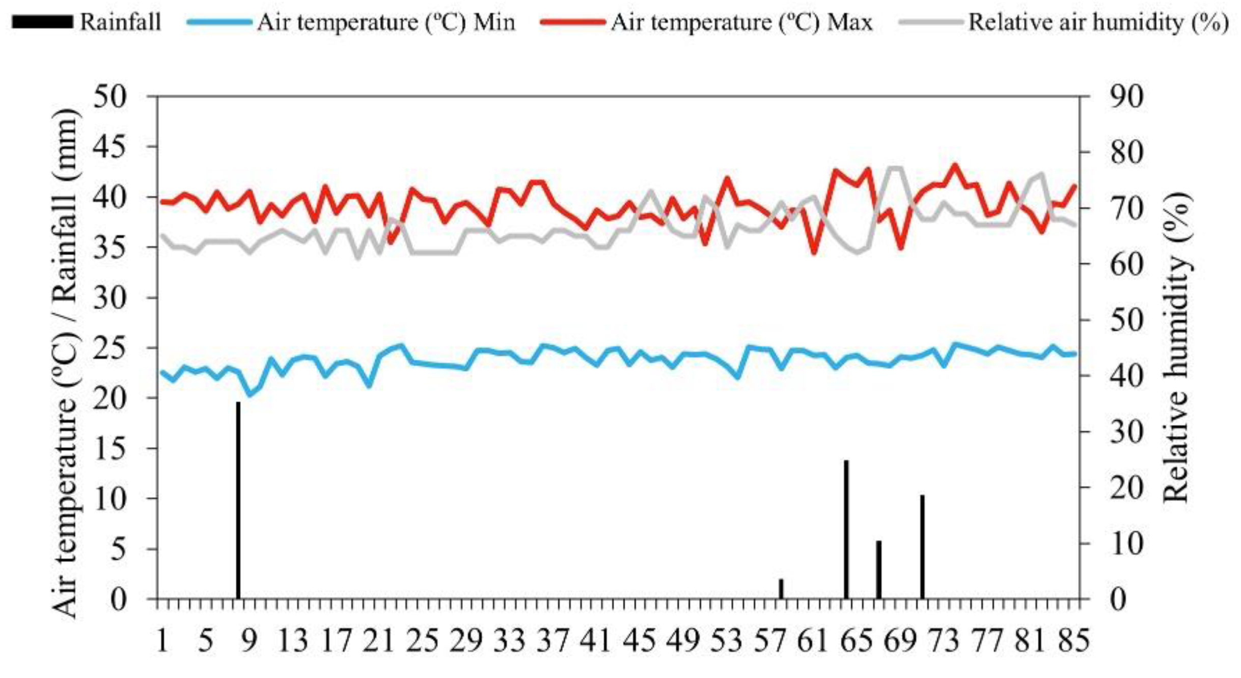
Figure 2.
Diagram of the experimental design showing (A) the composition and interaction of the study factors: electrical conductivity of the water, irrigation depths and inoculation, and (B) a timeline of the procedures carried out during the experiment.
Figure 2.
Diagram of the experimental design showing (A) the composition and interaction of the study factors: electrical conductivity of the water, irrigation depths and inoculation, and (B) a timeline of the procedures carried out during the experiment.
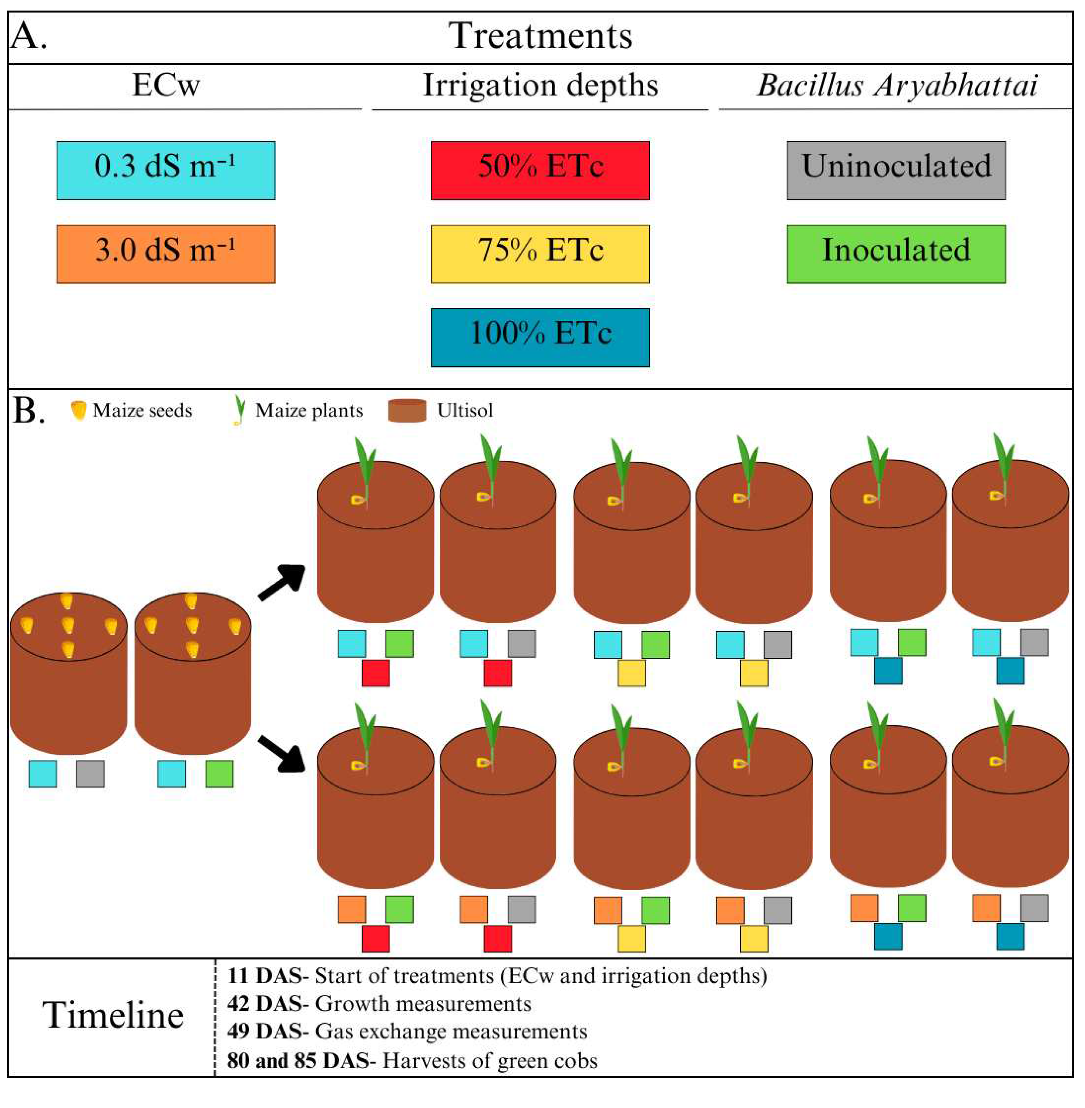
Figure 3.
Height in maize plants under different levels of electrical conductivity for the irrigation water, different irrigation depths, with and without inoculation, 42 days after sowing. Uppercase letters compare mean values between plants with and without inoculants, for the same electrical conductivity and irrigation depth by Tukey’s test (p ≤ 0.05). Error bars represent the standard error of the mean (n = 6).
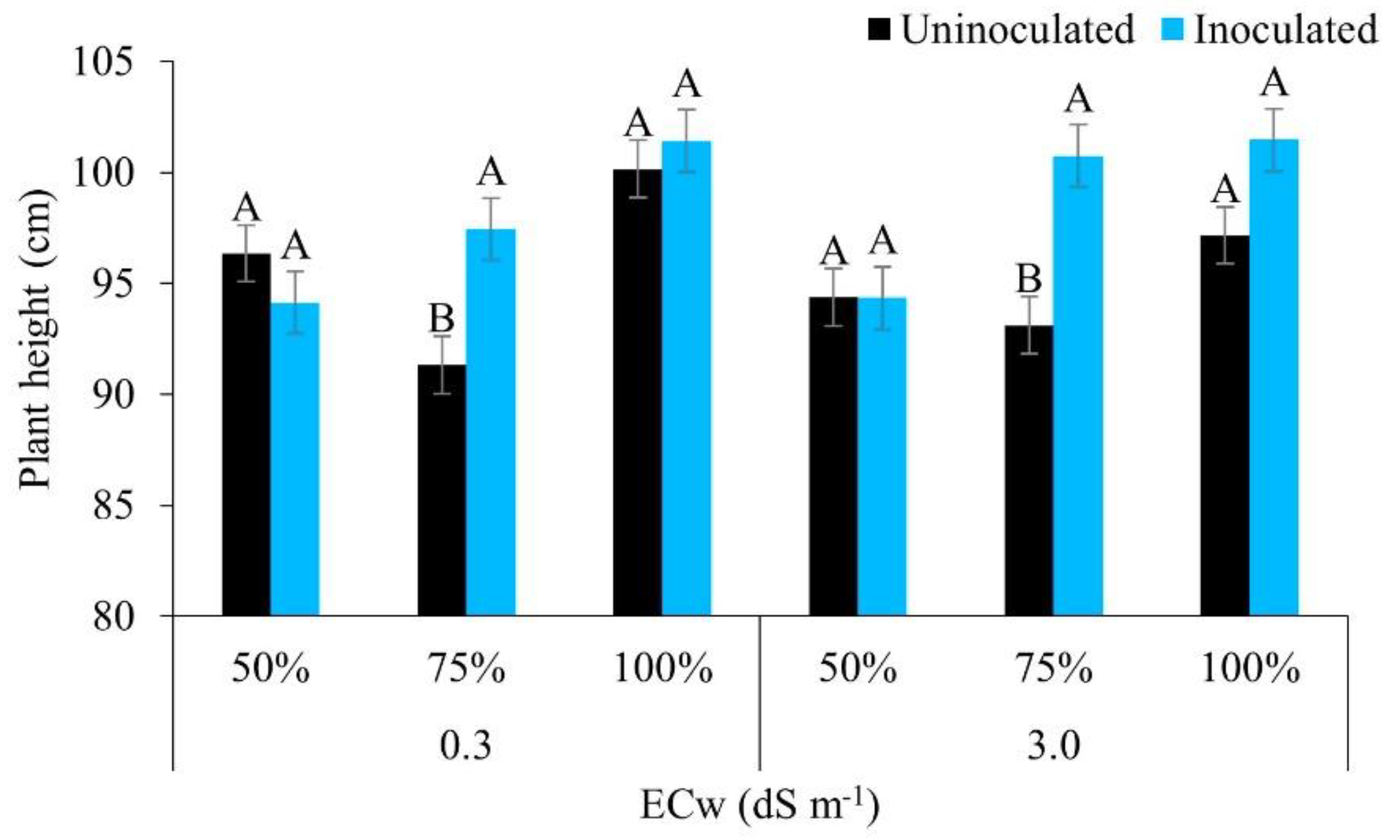
Figure 4.
Stem diameter in maize plants under different water regimes (A) and different levels of electrical conductivity for the irrigation water, with and without inoculation (B), 42 days after sowing. Figure A: Lowercase letters compare mean values by Tukey's test (p ≤ 0.05). Figure B: Lowercase letters compare mean values between ECw levels within each type of inoculation; uppercase letters compare mean values for the type of inoculation within each ECw by Tukey's test (p ≤ 0.05). Error bars represent the standard error of the mean (n = 6).
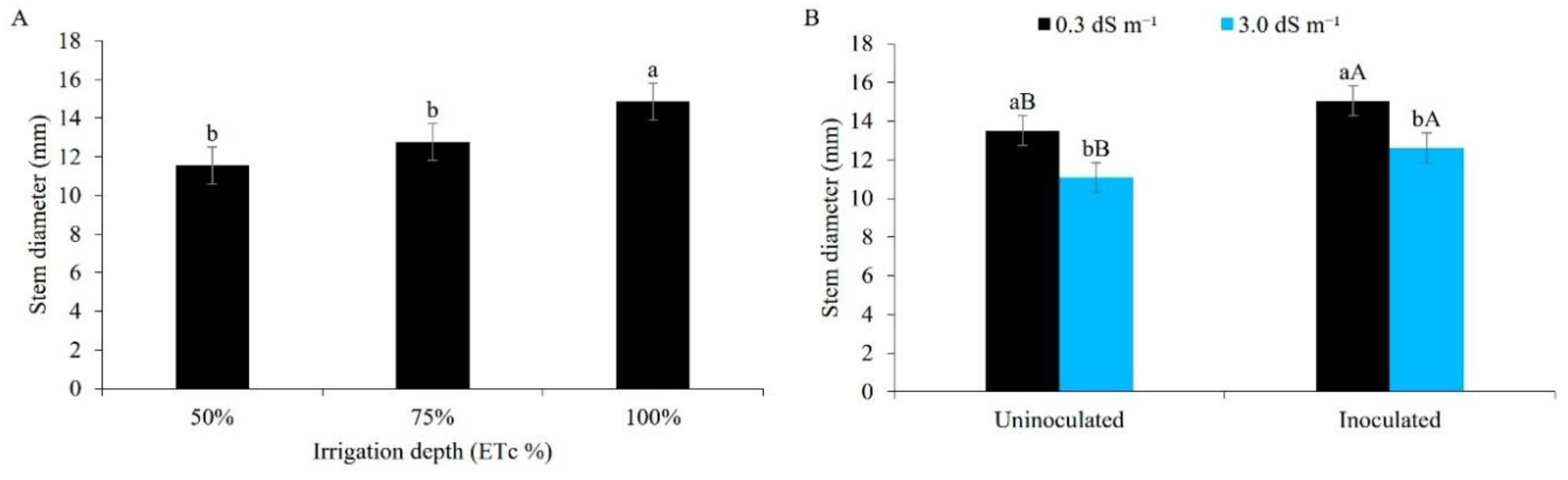
Figure 5.
Leaf area in maize plants under different levels of electrical conductivity for the irrigation water (A), and different irrigation depths, with and without inoculant (B), 42 days after sowing. Figure A: Lowercase letters compare mean values by Tukey's test (p ≤ 0.05). Figure B: Lowercase letters compare mean values between irrigation depths within each type of inoculation; uppercase letters compare mean values for the type of inoculation within each irrigation regime by Tukey's test (p ≤ 0.05). Error bars represent the standard error of the mean (n = 6).
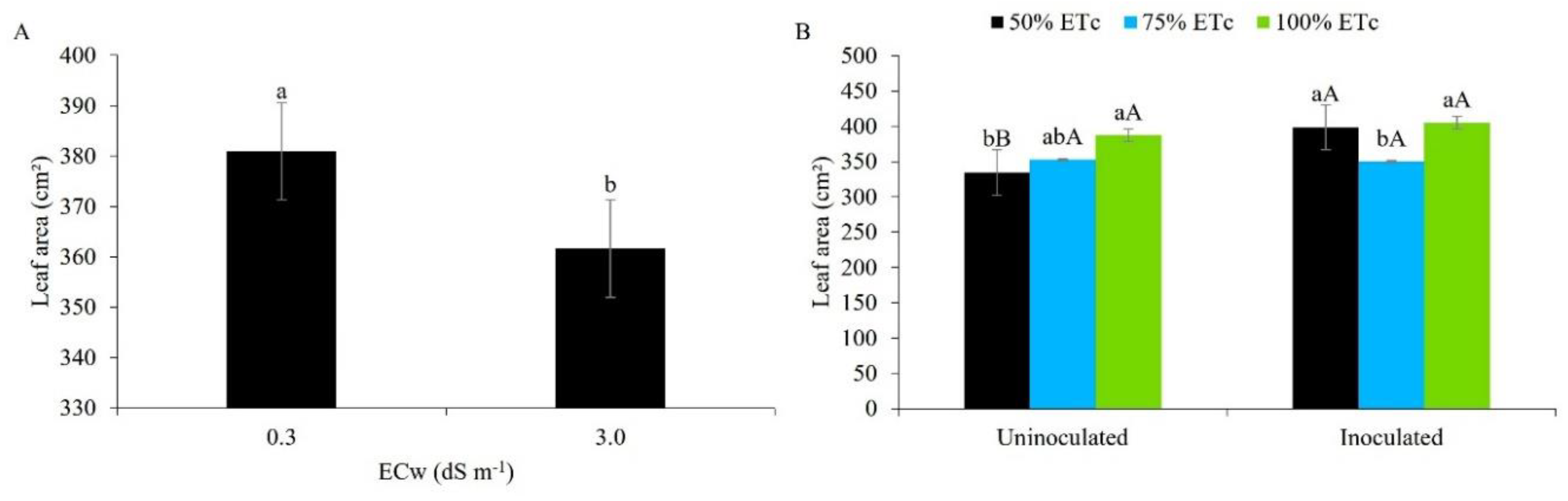
Figure 6.
Net photosynthetic rate (A) in maize plants under different levels of electrical conductivity for the irrigation water, with and without inoculation, 49 days after sowing. Lowercase letters compare mean values between ECw levels within each type of inoculation; uppercase letters compare means values for the type of inoculation within each ECw, by Tukey's test (p ≤ 0.05). Error bars represent the standard error of the mean (n = 6).
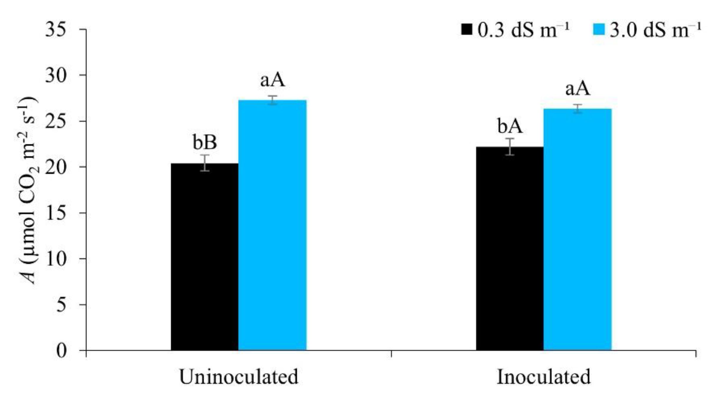
Figure 7.
Stomatal conductance (gs) in maize plants under different levels of electrical conductivity for the irrigation water and different water regimes, with and without inoculation, 49 days after sowing. Uppercase letters compare mean values between plants with and without inoculant within the same electrical conductivity and irrigation depth by Tukey’s test (p ≤ 0.05). Error bars represent the standard error of the mean (n = 6).
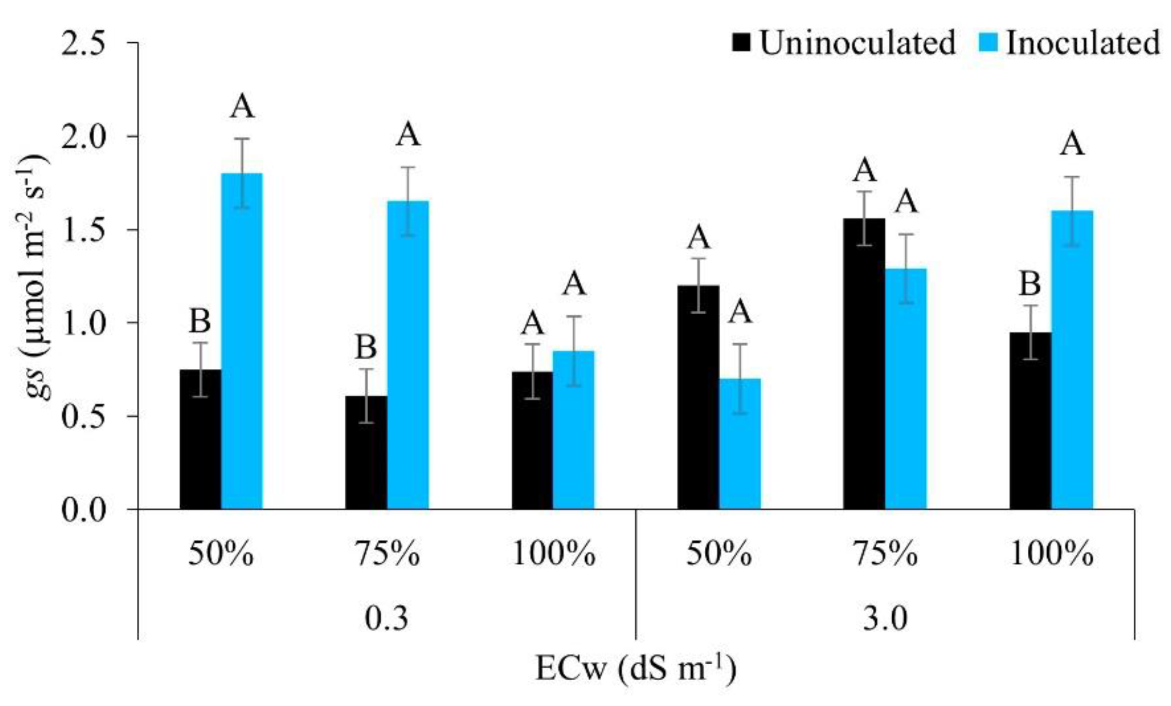
Figure 8.
Internal CO2 concentration (Ci) in maize plants under different levels of electrical conductivity for the irrigation water, with and without inoculation, 49 days after sowing. Lowercase letters compare mean values between ECw levels within each type of inoculation; uppercase letters compare mean values for the type of inoculation within each ECw, by Tukey’s test (p ≤ 0.05). Error bars represent the standard error of the mean (n = 6).
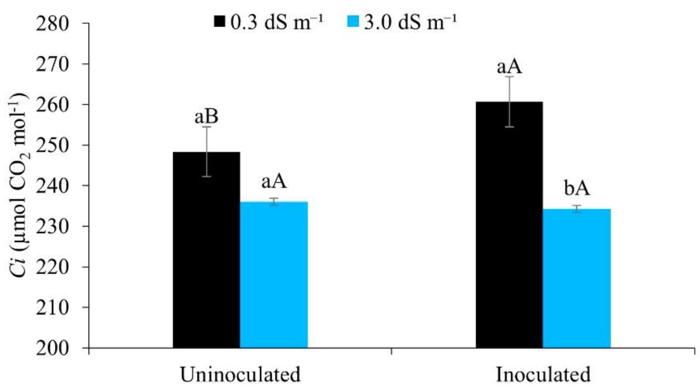
Figure 9.
Transpiration (E) in maize plants under different water regimes with and without inoculant, 49 days after sowing. Lowercase letters compare mean values between ECw levels within each water regime; uppercase letters compare mean values between water regimes at the same ECw, by Tukey’s test (p ≤ 0.05). Error bars represent the standard error of the mean (n = 6).
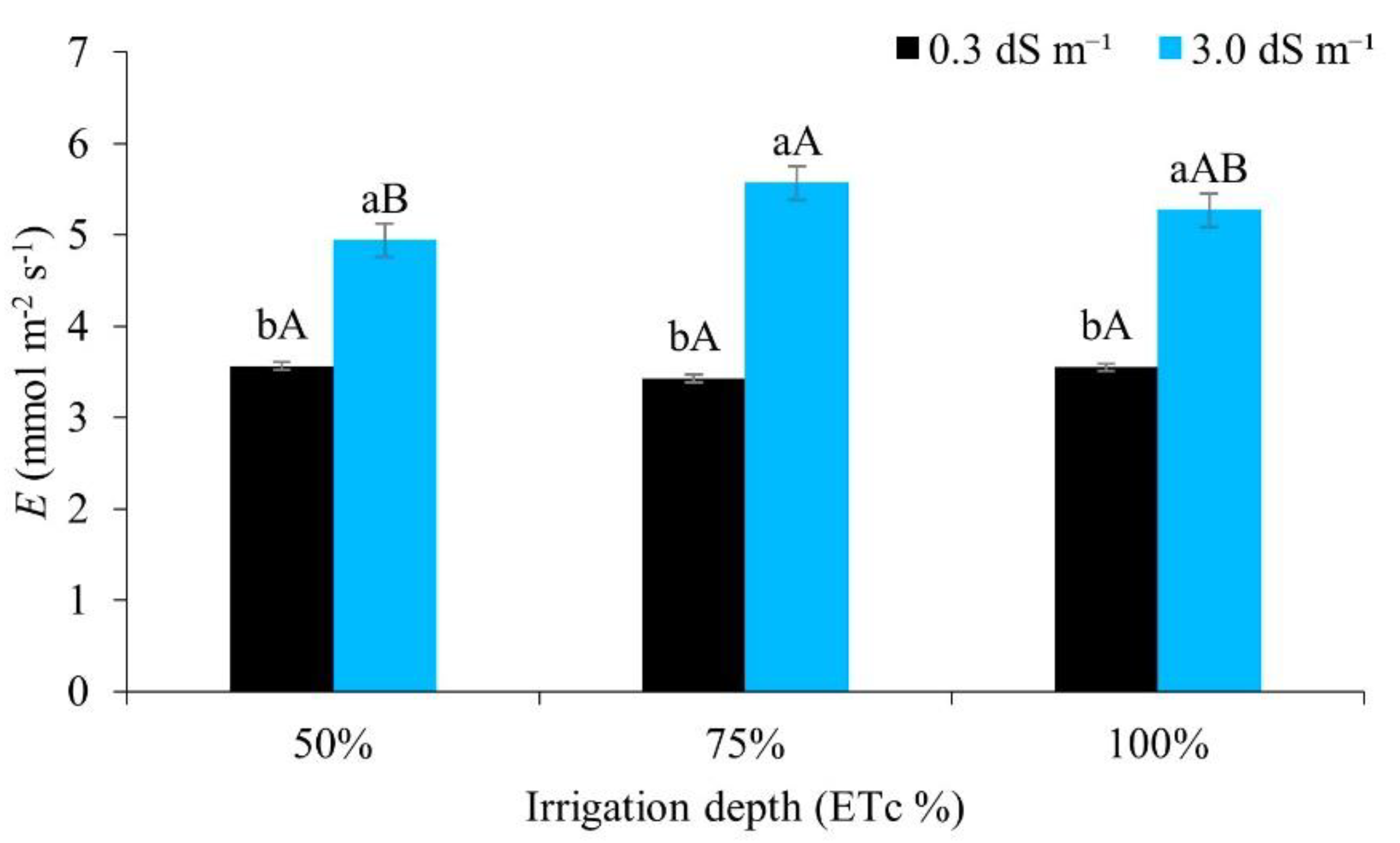
Figure 10.
Relative chlorophyll index (RCI) in maize plants under irrigation with water of different levels of electrical conductivity (A) and different water regimes (B), 49 days after sowing. Lowercase letters compare mean values by Tukey’s test (p ≤ 0.05). Error bars represent the standard error of the mean (n = 6).
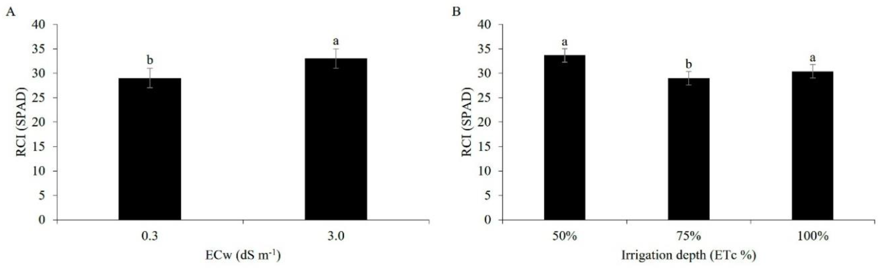
Figure 11.
Leaf temperature (LT) in maize plants under different levels of electrical conductivity for the irrigation water, different irrigation depths (A), and different water regimes, with and without inoculant (B), 49 days after sowing. Figure A: Lowercase letters compare mean values between ECw levels within each irrigation depth; uppercase letters compare mean values between irrigation depths at the same ECw by Tukey's test (p ≤ 0.05). Figure B: Lowercase letters compare mean values between irrigation depths within each type of inoculation; uppercase letters compare mean values between the types of inoculation within each irrigation depth by Tukey’s test (p ≤ 0.05). Error bars represent the standard error of the mean (n = 6).
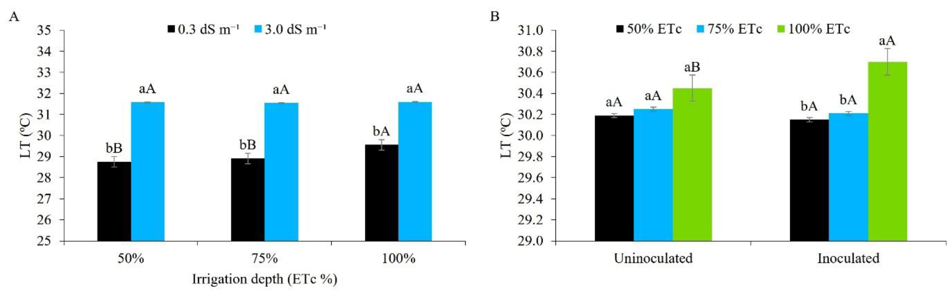
Figure 12.
Instantaneous water use efficiency (WUEi) in maize plants under different levels of electrical conductivity for the irrigation water, 49 days after sowing. Lowercase letters compare mean values by Tukey's test (p ≤ 0.05). Error bars represent the standard error of the mean (n = 6).
Figure 12.
Instantaneous water use efficiency (WUEi) in maize plants under different levels of electrical conductivity for the irrigation water, 49 days after sowing. Lowercase letters compare mean values by Tukey's test (p ≤ 0.05). Error bars represent the standard error of the mean (n = 6).
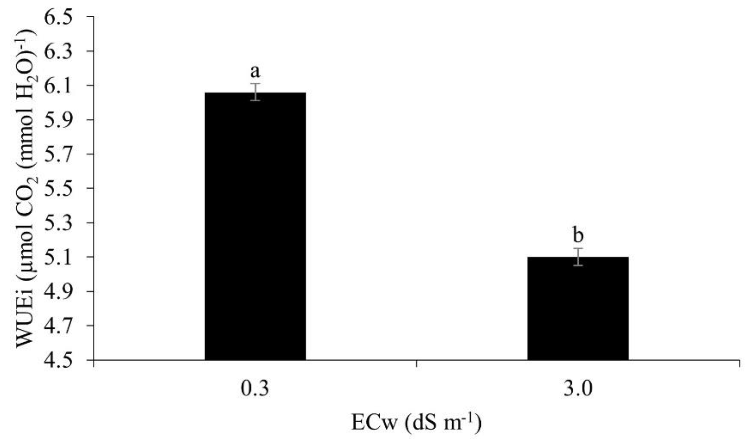
Figure 13.
Ear length in maize plants under different levels of electrical conductivity for the irrigation water, with and without inoculation (A), and different irrigation depths, with and without inoculation (B). Figure A: Lowercase letters compare mean values between ECw levels within each type of inoculation; uppercase letters compare mean values for the type of inoculation within each ECw, by Tukey's test (p ≤ 0.05). Figure B: Lowercase letters compare mean values between irrigation depths within each type of inoculation; uppercase letters compare mean values between the types of inoculation within each water regime, by Tukey's test (p ≤ 0.05). Error bars represent the standard error of the mean (n = 6).
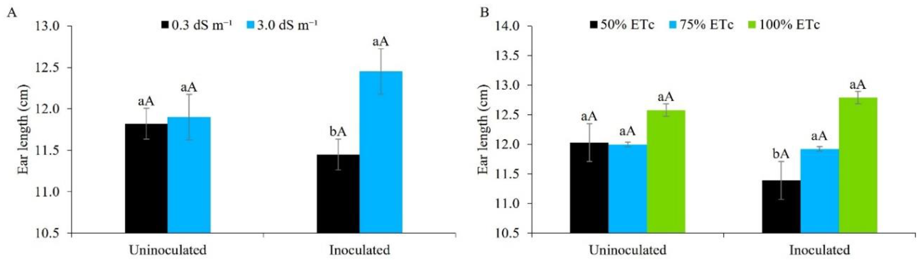
Figure 14.
Ear yield with straw (A) and ear yield without straw (B) in maize plants under different levels of electrical conductivity for the irrigation water, different irrigation depths, with and without inoculation. Uppercase letters compare mean values between plants with and without inoculant within the same electrical conductivity and irrigation depth by Tukey’s test (p ≤ 0.05). Error bars represent the standard error of the mean (n = 6).
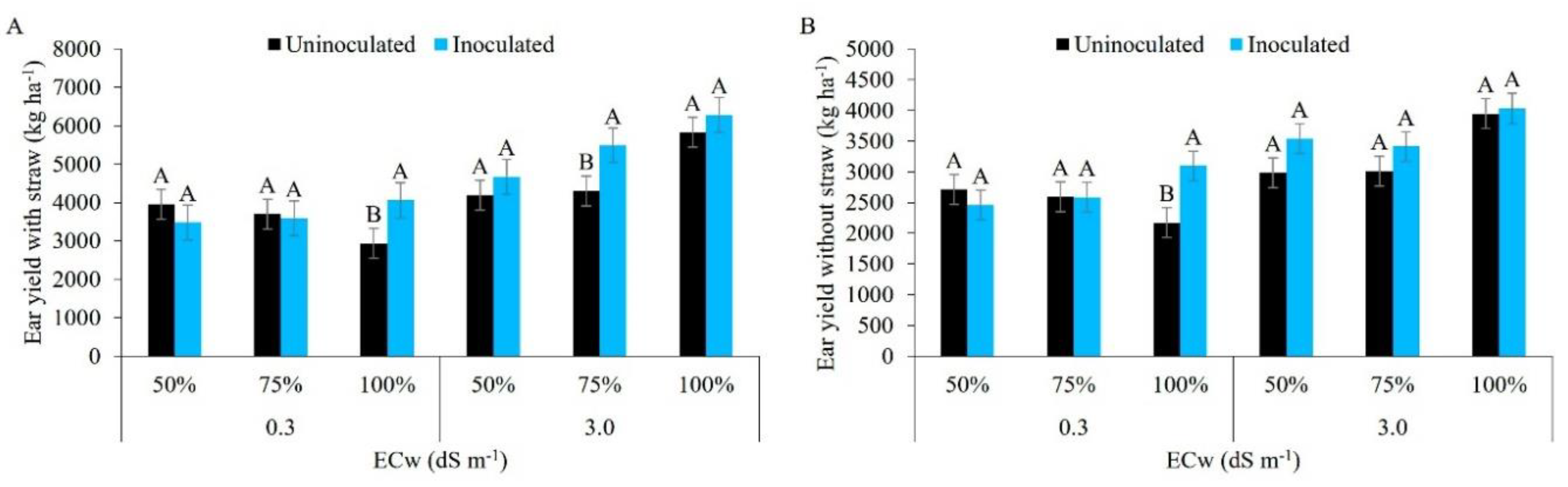

Table 1.
Chemical and physical characteristics of the soil sample before applying the treatments (0-20cm).
Table 1.
Chemical and physical characteristics of the soil sample before applying the treatments (0-20cm).
| pH | OM | N | C | P | Ca | Mg | Na | Al | H + Al | K | ECse | ESP | C/N | V | |
|---|---|---|---|---|---|---|---|---|---|---|---|---|---|---|---|
| H2O | ---------- g kg-1 ---------- | mg kg-1 | ----------------------- cmolc dm-3 ----------------------- | dS m-1 | % | % | |||||||||
| 5.6 | 11.59 | 0.71 | 6.72 | 20 | 3.20 | 2.60 | 0.07 | 0.35 | 2.15 | 0.17 | 0.76 | 1 | 9 | 74 | |
| SD (g cm-3) | CS | FS | Silt | Clay | Textural Classification | ||||||||||
| Bulk | Particle | ---------------------------------------- g kg-1 -------------------------------------- | |||||||||||||
| 1.31 | 2.61 | 507 | 283 | 133 | 77 | Loamy Sand | |||||||||
OM - Organic matter; ESP - Percentage of exchangeable sodium; ECse - Electrical conductivity of the soil saturation extract; V - Base saturation; SD - Soil density; CS - Coarse sand; FS - Fine sand.
Table 2.
Total irrigation depth applied in each treatment.
| ECw (dS m-1) |
ETc (%) |
Total depth applied (mm) | |
|---|---|---|---|
| Uninoculated | Inoculated | ||
| 0.3 | 50 | 260.4 | 260.4 |
| 75 | 390.6 | 390.6 | |
| 100 | 520.8 | 520.8 | |
| 3.0 | 50 | 260.4 | 260.4 |
| 75 | 390.6 | 390.6 | |
| 100 | 520.8 | 520.8 | |
Table 3.
Chemical characterisation and classification of the irrigation water used in the experiment.
Table 3.
Chemical characterisation and classification of the irrigation water used in the experiment.
| ECw | Ca2+ | Mg2+ | K+ | Na+ | Cl- | HCO3- | pH | CE | SAR | Classification¹ |
|---|---|---|---|---|---|---|---|---|---|---|
| dS m-1 | ---------mmolc L-1-------- | ---mmol L-1--- | in H2O | dS m-1 | (mmolc L-1)0,5 | |||||
| 0.3 | 0.6 | 1.4 | 0.2 | 0.4 | 2.5 | 0.1 | 6.9 | 0.3 | 0.4 | C2S1 |
| 3.0 | 6.33 | 7.64 | 2.0 | 15.6 | 25 | 1.0 | 7.79 | 3.0 | 5.9 | C4S2 |
1 - [32]; SAR - Sodium adsorption ratio.
Table 4.
Chemical characterisation of the organic fertilisers used in the experiment.
| Organic source | N | P | K+ | Ca2+ | Mg2+ |
|---|---|---|---|---|---|
| g L-1 | |||||
| Cattle manure | 0.96 | 0.47 | 0.59 | 1.10 | 0.25 |
| Cattle biofertiliser | 0.82 | 1.4 | 1.0 | 2.5 | 0.75 |
Table 5.
Summary of the analysis of variance for plant height (PH), number of leaves (NL), stem diameter (SD), and leaf area (LA), in maize plants under different levels of electrical conductivity for the irrigation water (ECw), irrigation depths (ID) and inoculation (INOC), 42 days after sowing.
Table 5.
Summary of the analysis of variance for plant height (PH), number of leaves (NL), stem diameter (SD), and leaf area (LA), in maize plants under different levels of electrical conductivity for the irrigation water (ECw), irrigation depths (ID) and inoculation (INOC), 42 days after sowing.
| Source of Variation | DF | Mean Square | |||
|---|---|---|---|---|---|
| PH | NL | SD | LA | ||
| Blocks | 5 | 29.67ns | 1.95ns | 1.53ns | 207.38ns |
| ECw | 1 | 0.06ns | 2.60ns | 87.96** | 5613.37* |
| Residual (ECw) | 5 | 27.97 | 0.61 | 2.74 | 412.05 |
| Irrigation depths (ID) | 2 | 21.30ns | 0.40ns | 56.08** | 10546.35** |
| Residual (ID) | 20 | 15.37 | 0.43 | 2.49 | 974.55 |
| Inoculation (INOC) | 1 | 9.56ns | 0.33ns | 35.25** | 10360.73** |
| Residual (INOC) | 30 | 16.57 | 0.54 | 3.05 | 1161.23 |
| ECw × ID | 2 | 160.75** | 0.25ns | 1.87ns | 2864.11ns |
| ECw × INOC | 1 | 149.91** | 0.004ns | 0.0007* | 2064.59ns |
| ID × INOC | 2 | 0.24* | 0.16ns | 0.27ns | 5769.978* |
| ECw × ID × INOC | 2 | 70.49* | 1.42ns | 4.56ns | 654.36ns |
| CV (%) - Ecw | 5.46 | 9.49 | 12.68 | 5.47 | |
| CV (%) - ID | 4.05 | 7.97 | 12.08 | 8.41 | |
| CV (%) - INOC | 4.20 | 8.95 | 13.37 | 9.18 | |
DF: Degrees of freedom; CV: Coefficient of variation; ns, *, and **: not significant, significant at p ≤ 0.05 and significant at p ≤ 0.01, respectively.
Table 6.
Summary of the analysis of variance for photosynthesis (A), stomatal conductance (gs), internal CO2 concentration (Ci), transpiration (E), relative chlorophyll index (RCI), leaf temperature (LT) and instantaneous water use efficiency (WUEi), in maize plants under different levels of electrical conductivity for the irrigation water (ECw), different irrigation depths (ID), and inoculation (INOC), 49 days after sowing.
| Source of Variation | DF | Mean Square | ||||||
|---|---|---|---|---|---|---|---|---|
| A | gs | Ci | E | RCI | LT | WUEi | ||
| Blocks | 5 | 9.03ns | 0.67ns | 798.40ns | 0.43** | 10.05ns | 3.67ns | 0.006* |
| ECw | 1 | 361.19** | 0.15ns | 4504.68* | 36.83** | 191.12** | 74.72** | 11.07** |
| Residual (ECw) | 5 | 7.25 | 0.16 | 303.63 | 0.00** | 2.94 | 0.61 | 0.28 |
| Irrigation depths (ID) | 2 | 2.14ns | 0.26ns | 315.25ns | 0.25ns | 92.35* | 0.77* | 0.22ns |
| Residual (ID) | 20 | 8.90 | 0.14 | 101.83 | 0.11 | 23.43 | 0.15 | 0.15 |
| Inoculation (INOC) | 1 | 2.13ns | 3.60** | 336.02ns | 0.11ns | 39.45ns | 0.04* | 0.01ns |
| Residual (INOC) | 30 | 3.13 | 0.18 | 110.47 | 0.16 | 9.78 | 0.02 | 0.21 |
| ECw × ID | 2 | 2.86ns | 1.46** | 9.75ns | 0.58* | 66.17ns | 0.67* | 0.01ns |
| ECw × INOC | 1 | 6.97* | 2.48** | 595.02* | 0.47ns | 0.09ns | 0.04ns | 0.008ns |
| ID × INOC | 2 | 1.88ns | 0.04ns | 234.33ns | 0.27ns | 4.97ns | 0.10* | 0.006ns |
| ECw × ID × INOC | 2 | 0.78ns | 2.57** | 110.47ns | 0.18ns | 0.87ns | 0.02ns | 0.27ns |
| CV (%) - ECw | 11.20 | 11.85 | 6.34 | 0.77 | 5.54 | 2.59 | 9.60 | |
| CV (%) - ID | 12.41 | 10.04 | 3.67 | 7.88 | 15.62 | 1.32 | 7.03 | |
| CV (%) - INOC | 7.37 | 14.05 | 3.82 | 9.11 | 10.09 | 0.50 | 8.31 | |
DF: Degrees of freedom; CV: Coefficient of variation; ns, *, and **: not significant, significant at p ≤ 0.05 and significant at p ≤ 0.01, respectively.
Table 7.
Summary of the analysis of variance for ear length (EL), ear diameter (ED), ear yield with straw (EYWS) and ear yield without straw (EYWoS), in maize plants under different levels of electrical conductivity for the irrigation water (ECw), different irrigation depths (ID), and inoculation (INOC).
| Source of Variation | DF | Mean Square | |||
|---|---|---|---|---|---|
| EL | ED | EYWS | EYWoS | ||
| Blocks | 5 | 3.09ns | 17.63ns | 6772473.13ns | 3162178.48ns |
| ECw | 1 | 5.15ns | 9.90ns | 40862788.82** | 14079648.00** |
| Residual (ECw) | 5 | 1.69 | 4.58 | 1711897.76 | 820739.41 |
| Irrigation depths (ID) | 2 | 1.35ns | 5.27ns | 3121961.40ns | 1275678.96* |
| Residual (ID) | 20 | 1.49 | 3.63 | 1464975.55 | 351695.38 |
| Inoculation (INOC) | 1 | 0.14ns | 0.38ns | 3533704.78** | 450274.80* |
| Residual (INOC) | 30 | 0.86 | 1.96 | 363835.20 | 309105.44 |
| ECw × ID | 2 | 0.34ns | 1.57ns | 5385095.95* | 1002466.33ns |
| ECw × INOC | 1 | 3.78* | 2.51ns | 1257793.16ns | 69497.37ns |
| ID × INOC | 2 | 6.11** | 1.65ns | 956622.93ns | 225383.24ns |
| ECw × ID × INOC | 2 | 1.27ns | 5.31ns | 1678902.68* | 1118325.91* |
| CV (%) - ECw | 10.92 | 6.24 | 29.91 | 29.74 | |
| CV (%) - ID | 10.24 | 5.56 | 27.67 | 19.47 | |
| CV (%) - INOC | 7.80 | 4.08 | 13.79 | 18.25 | |
DF: Degrees of freedom; CV: Coefficient of variation; ns, *, and **: not significant, significant at p ≤ 0.05 and significant at p ≤ 0.01, respectively.
Disclaimer/Publisher’s Note: The statements, opinions and data contained in all publications are solely those of the individual author(s) and contributor(s) and not of MDPI and/or the editor(s). MDPI and/or the editor(s) disclaim responsibility for any injury to people or property resulting from any ideas, methods, instructions or products referred to in the content. |
© 2023 by the authors. Licensee MDPI, Basel, Switzerland. This article is an open access article distributed under the terms and conditions of the Creative Commons Attribution (CC BY) license (https://creativecommons.org/licenses/by/4.0/).
Copyright: This open access article is published under a Creative Commons CC BY 4.0 license, which permit the free download, distribution, and reuse, provided that the author and preprint are cited in any reuse.


