Submitted:
27 February 2023
Posted:
27 February 2023
You are already at the latest version
Abstract
The cost to train a basic qualified U.S. Navy fighter aircraft pilot is nearly $10M. The training includes primary, intermediate, and advanced stages, with the advanced stage involving extensive flight training and being very expensive as a result. Despite the screening tests in place and early-stage attrition taking place, 4.5% of aviators undergo attrition in this most expensive stage. Key reasons for aviator attrition include poor flight scores, voluntary withdrawals, and medical causes. Reduction in late-stage attrition offers several financial and operational benefits to the U.S. Navy. To that end, this research leverages feature extraction and machine-learning techniques on the very sparse flight test grades of student aviators to identify those with a high risk of attrition early in training. Using about 10 years of historical U.S. Navy pilot training data, trained models accurately predicted 50% of attrition with a 4% false positive rate. Such models could help the U.S. Navy save nearly $20M a year in attrition costs. In addition, machine-learning models were trained that can recommend a suitable training aircraft type for each student aviator. These capabilities could help better answer the need for pilots and reduce the time and cost to train them.
Keywords:
Pilot Training
; Machine Learning
; Attrition Prediction
; Aircraft Suitability
; Cost Savings
; Automation
1. Introduction & Motivation
The U.S. Navy’s Chief of Naval Air Training (CNATRA) trains nearly 1,100 pilots every year in six training pipelines (strike, helo, tilt-rotor, and others) to fly different Navy aircraft. The six training pipelines are shown in Figure 1. Student aviators are assigned to those pipelines based on their performance in primary-stage training, the needs of the Navy, students’ preference, and the availability of training slots. During the course of training, student aviators undergo primary, sometimes intermediate, and advanced training stages depending on the assigned aircraft pipeline. Student aviators that successfully complete the advanced training stage receive “Wings of Gold” to become naval aviators i.e., qualified Navy pilots.
Pilot training is expensive and includes training on both sophisticated simulators and real aircraft, as well as the involvement of several instructors, schedulers, and others. The cost of training increases as student aviators advance through the stages and have increasing flight training. Despite the many screenings and early-stage attrition, 4.5% of advanced-stage aviators undergo attrition in this most expensive training stage. Reasons for aviator attrition include flight failure, academic failure, voluntary withdrawal (Drop on Request - DOR), medical failures, and others [1]. The distribution of attrition in primary, intermediate, and advanced stages by reason for attrition is shown in Figure 2. Figure 2 shows that, with the exception of the primary stage, flying-related reasons are predominant. Indeed, more than 50% of the attrition in the intermediate and advanced stages of training is reported as due to reasons related to poor flight scores.
DOR is the most observed reason for attrition in the primary training stage with lack of flying competency being a close second. As illustrated in Figure 3, 90% of DOR-related attrition occur in the first two quarters of primary training, while 60% and 80% of the attrition in the third and fourth quarters respectively, are due to a lack of flying competency. Figure 3 shows that attrition related to lack of flight competency represents more than 50% of estimated primary-stage attrition costs.
As illustrated in Figure 4, the cost to CNATRA and the U.S. Navy for each advanced stage student attrition is several times higher than that for those in the primary stage. This is due to the fact that the direct cost of attrition of each student is equivalent to the sum of all the costs of training received by the student up to that point. In addition, the amount of flight time as well as the cost per flight hour during the advanced training stage are much higher than during the primary training stage. Figure 4 shows the estimated direct cost of attrition of a strike pipeline student aviator in the primary, intermediate, and advanced training stages [3,4]. In particular, it shows that, for the strike pipeline, 4.5% of the students experience attrition in the advanced stage, where the cost of each attrition is $2M. Accordingly, by identifying such students during primary stage and preventing their advanced stage attrition, the U.S. Navy could save up to an estimated $1.7M for each student accurately identified. In addition, the late-stage attrition causes delays in meeting the U.S. Navy’s pilot demand [5].
Consequently, the goal of this research is to develop a data-driven approach informed by machine-learning techniques to predict the likelihood that a student aviator will not complete training. Making such predictions, though critical, is a challenging task due mainly to the many factors that affect the training process as well as the existence of different future scenarios. Section 2 discusses previous attempts at predicting student aviator attrition. Section 3 presents the approach proposed and its implementation as a means to address the aforementioned research objective. Section 4 analyzes and discusses the results. Finally, Section 5 concludes on the work conducted and discusses avenues for future work.
2. Background
While the U.S. Navy does an effective job at screening applicants for flight training through the Aviation Selection Test Battery (ASTB), a considerable percentage of selected applicants still undergo attrition, during training, for a variety of reasons. All-phase CNATRA attrition rates averaged 17% for Student Naval Aviators (SNA) and 23% for Student Naval Flight Officers (SNFO). Between 2003 and 2007, CNATRA reported 1,558 cases of student attrition [1]. Studies on what factors contribute to and help predict a student aviator’s success or risk of attrition have been ongoing for several decades [6,7,8,9,10,11,12]. These studies aimed to find statistical correlations between a pilot’s performance and other measures. However, many of their findings, if implemented, would have resulted in the rejection of many successful aviators as well [13,14]. These studies also reported on the challenges associated with the data used to make predictions, and in particular, the large number of influencing features and the sparsity of the data sets [15].
Compounded to the high attrition rate is the acute shortage in pilots in both the U.S. defense and commercial aviation sectors [16]. As a result, Defense agencies in the U.S. have been looking for solutions to reduce the time and cost to train pilots and meet the demand quickly. The new Naval Introductory Flight Evaluation (NIFE) program’s aeronautical adaptability screening is designed to identify concerns like motion sickness and anxiety early on to decrease DOR seen in 40% of student aviators that experienced attrition [17]. Still, 24% of the attrition was due to failing to meet flight competency levels and 9% was due to academic failure.
Collecting and analyzing instructor-given scores for different flight and academic tests and events is a feasible approach to predict the risk of attrition in later training stages. The recent improvements in machine-learning techniques as well as their ability to learn complex relationships between features, even in the case of missing data, make them a great candidate for this problem [18]. An example of such studies includes the use of linear regression models on U.S. Air Force pilot training data to provide guidance on the selection of students for each class [19]. The results suggested grouping students with similar numbers of flight-hours. Jenkins et.al. [18] leveraged different traditional and deep learning models on U.S. Air Force pilot training preliminary tests and previous flight experience data to determine whether a candidate would successfully complete pilot training. Results showed that ensemble tree-based approaches had a top classification accuracy of 94%. Based on their findings, the authors proposed a composite pilot selection index to be used to select candidates for pilot training.
Machine-learning techniques have also been applied and evaluated on U.S. Naval pilot training datasets. Erjevac [3] predicted the probability of success in primary stage training using decision tree-based methods at three stages (1. entry into flight school, 2. completion of Initial Flight School (IFS), and 3. completion of Aviation Pre-flight Indoctrination (API)). The models were trained on students trained between 2013 and 2018 using student features available from before the start of their training. Hence, the author suggested that the models could be used as a screening tool to avoid selecting applicants with a low probability of success. Another effort [2] used features generated from ASTB, IFS and API training of nearly 15,000 students aviators to predict the success in primary, intermediate and advanced stages of training. The author reported that machine-learning models such as multiple logistics, decision trees, random forests, and generalized linear models only explained a small amount of variation in training success or failure. It was also stated that ASTB scores had very little to no effect on predicting success in primary and advanced training. A different effort [20] looked at flight and academic test scores and collected features of nearly 19,000 student aviators across ASTB, IFS, primary, intermediate, and advanced training stages, and Fleet Replacement Squadron (FRS). Many challenges to applying machine-learning algorithms were reported, including the format in which flight and academic event data were being stored, missing data, as well as the lack of suitable features. Finally, Phillips et al. [21] extracted correlations between highly aggregated test score features and flight training success metrics such as Naval Standardized Scores.
Overall, the research studies published so far either use early-stage training data for screening and primary training stage success prediction or do not generate satisfactory results for intermediate and advanced-stage success prediction. Another shortcoming is the lack of methods capable of ingesting and pre-processing primary stage flight grades data at the flight item level without losing potentially useful information.
In this study, data-preprocessing and feature extraction methods that enable ingestion of flight and academic grades data at any point during primary stage training are developed. These features are then utilized to train and test different machine-learning models to predict the outcome of primary, intermediate, and advanced training stages. In addition, a pipeline suitability score is developed that recommends what aircraft platform might best fit a student aviator based on their primary training test scores. Finally, an attrition cost estimation model is developed that demonstrates that implementing these methods could significantly benefit CNATRA by reducing attrition costs and enabling more effective utilization of training resources.
3. Materials and Methods
The steps followed as part of this approach aim at predicting the risk of attrition and at generating pipeline suitability scores for Naval student aviators. As such, they are typical of a data science approach and include the identification and ingestion of relevant and available datasets, the pre-processing and extraction of features of interest and the training and testing of a number of machine-learning models. Each of these steps are discussed in detail below.
3.1. Datasets
Primary training stage academic and flight item grades were provided in .csv format for nearly 8,000 naval student aviators that were trained in between 2012 and 2019. The academic and flight tests given to students are dependent on the syllabus followed, and changes to syllabus over the years resulted in differences in the number and type of available flight and academic graded items. Information about training outcomes for the student aviators in primary, intermediate, and advanced stages of training was also made available as additional .csv sheets. Each student in these tables was identified with a unique "ID_CODE" number, which was used when merging related sheets. An overview of the different datasets leveraged for the purpose of this work is provided in Figure 5 and further discussed in the sections below.
3.1.1. Flight Grades Data
Ten .csv sheets were related to primary stage data which included primary stage syllabus status, attrition reason if any, syllabus-event names, flight hours, flight-item grades, and the Maneuver Item File ("MIF") data. The primary stage training included flight events such as "abort take-off," "arcing," and about 140 others with small differences from one syllabus to another. The ten tables were concatenated using the student IDs. A small number of students had been trained in more than one syllabus and were eliminated from the analysis. The flight grades were given on a scale of 1 to 5.
3.1.2. Academic Grades Data
For each student, about 100 entries were available, each corresponding to a syllabus event such as C2101. In many instances, a syllabus event was repeated due to an incompletion or the first instance being a warm-up event. In each entry, instructors tested and provided grades for only one or a small number of flight-graded items. Hence, most of the columns in each row were empty, resulting in the data being extremely sparse. To address this challenge and facilitate the use of data by machine-learning models, aggregation and feature extraction were performed which required input from subject matter experts. Eight .csv sheets with academic test grades were available. Most students in these tables had one row entry each with many columns filled for each academic grade obtained. However, academic test grades were not considered in the analysis for two reasons: 1) the large variance in the number of grades available for each student and, 2) academic failure not being the primary reasons for attrition.
3.1.3. Training Outcomes Data
Three tables with information on training outcomes at the primary, intermediate, and advanced stages of training were available. These tables included information such as student ID, aircraft pipeline assigned, syllabus completion status, and Naval Standardized Scores (NSS). For the students who were unsuccessful, the reason for attrition was also provided. For the purpose of this effort the completion status (attrite or successful) from different training stages were used to generate the targets for the attrition risk prediction and the pipeline recommendation models. Overall, about 10,000 unique student IDs were recorded with approximately 9,000, 3,000, and 6,000 students IDs available in primary, intermediate, and advanced training datasets, respectively. Among them, 2,243 unique IDs were present in both primary and intermediate datasets and 5,262 unique IDs were present in both primary and advanced datasets, as shown in Figure 6. The entries that are common to the flight grades and outcomes datasets provide both features and targets to train the machine-learning models. However, the syllabus completion status in each training stage is not directly used. The objective of the classification machine-learning models is to differentiate students who would complete all phases of training from those who would not (i.e., those who do/would not finish all stages of the training). Identifying the particular training stage at which a student would drop is not addressed as part of this effort. Finally, flight proficiency and skills required for different aircraft pipelines are different. Consequently, using intermediate and advanced stage syllabus completion status as targets, without pipeline information, is not optimal. As a result, pipeline recommender models, which indicate the suitability of a student for a particular aircraft, were also developed. These models are specific to each pipeline and use corresponding training completion status as targets.
3.2. Data Cleansing and Features Extraction
The datasets originated from different sources and required standardization and cleaning. The data has both numeric and nominal features, spelling errors, and multiple formatting styles, which were standardized. For example, some entries in the advanced stage syllabus track are “Adv_Stk”, while some are “ADV_STK”. One-hot integer encoding was used for categorical features. Through exploratory data analysis, such corrections were made, and outliers and erroneous inputs were removed.
The data that would be available for a student aviator at different points in training was identified along with the corresponding target(s) for prediction. At any selected point during training, a set of features and a target provide the data necessary to train a supervised machine-learning model.
- For the attrition prediction models: the syllabus completion status, which takes two values: “Complete” or “Attrite”, according to whether a student successfully completed all stages of training or not was used as the target.
- For the pipeline recommender models: each machine-learning model pertained to one aircraft pipeline. For a selected aircraft pipeline, the student aviators that were successful were given a positive label and all other students were given a negative label, indicating that they were not suitable for that pipeline. Models trained using data labeled in this way would try to mimic the current selection process.
Eighty-five percent of the 90 million cells in the concatenated flight grades table (600,000 rows and 140 columns) were empty. As a result, an aggregation and feature extraction strategy was needed so as to not lose key information. It is expected that a grade given by an instructor for a flight-graded item is indicative of the proficiency for that maneuver/skill, such as landing, take-off, headwork, and nearly 140 others. Following inputs from subject matter experts, the data was aggregated according to flight-graded items to capture maneuver/skill-specific proficiency levels as observed by flight instructors.
In particular, statistical features were generated from the multiple non-zero entries in each column for each student aviator. Five features: average, count, minimum, maximum, and trend over time, were calculated and stored for the flight graded items type columns. Other features such as total flight hours, number of days in training, the total number of events, failure rate, and others, were extracted from other columns, as shown in Figure 7. Overall, this resulted in about 700 features for each of 7,465 student aviators in the primary flight grades datasets. Still, 10% of the cells were empty, which can be accommodated by some machine-learning models. The reduction in empty cells by aggregation and feature extraction processes is shown in Figure 8, where white areas represent empty cells. Further, columns with only one unique value were eliminated and empty cells were filled in with the mean values of the corresponding columns.
Features datasets were also generated utilizing flight grades available only from the first quarter and up to the second and third quarters of primary training. The split into different quarters was performed based on the average number of events required by each student aviator to successfully complete primary-stage training. This allows for a more continuous attrition risk monitoring. The potential cost savings achieved through accurate attrition prediction is also more precisely calculated as attrition during Q-3 or Q-4 (third or fourth quarter) of the primary stage is more expensive than attrition during Q-1 or Q-2. For example, machine-learning models estimating the risk of attrition between the end of Q-1 and the end of the advanced training stage were trained using only Q-1 grades. Machine-learning models were also trained with all of the primary flight grade data and additional pipeline information from intermediate and advanced stages, when available, to estimate the risk of attrition. Flight grades from the intermediate and advanced stages, if available, should be used for the end of intermediate and advanced stages models to predict attrition in the advanced stage and Fleet Replacement Squadron (FRS) stage, respectively. The different models and the timeline at which they are to be used are depicted in Figure 9. Table 1 summarizes the data which was available and leveraged as part of this effort, along with the targets that the models would predict at the different training timelines.
3.3. Training Machine-Learning Models
The attrition risk prediction is approached as a binary supervised classification problem, with the probability of a positive classification (0 to 1) being used as the attrition risk score. In binary classification problems, class imbalance can be a challenge. Class imbalance refers to a significant difference in the number of positive class labels (student attrition) and negative class labels (successful students) as targets. The attrition rates in each of the three (primary, intermediate, and advanced) training stages varied between 3 and 8 percent in the provided datasets. Since machine-learning models perform better with close to equal distribution of class labels, advanced sampling strategies such as adaptive-synthetic (ADASYN) oversampling [22] and random undersampling (RUS) [23] were used in different models to reduce the class imbalance. Similarly, the pipeline recommender models were also framed as binary supervised classification problems, and undersampling and oversampling techniques were tested.
Many different types of machine-learning classification-models can be used to demonstrate the aforementioned approach and objectives. Results for relatively simple classifiers to advanced models combined with sampling techniques are generated and reported in this paper. Tested models include logistic regression, support vector machines (SVM), K-nearest neighbors (k-NN), decision trees, random forests, gradient boosting, XGBoost, light gradient boosting machines, and multi-layer perceptrons (MLP). A five-fold data split that randomly allocates 80% of the data to train the models and 20% to test them was implemented. To evaluate and compare the performance of the models, performance metrics that not only consider the accurate identification of attriting students (true positives) but also penalize false positives are needed. If a policy of proactive removal of students with a high risk of attrition is implemented, a false positive prediction would lead to additional costs equal to that needed to retrain another student to the same stage who would go on to be successful. In order to more precisely calculate the savings and additional costs due to accurate attrition prediction or false positives, true positive and false positive metrics were further classified based on when the attrition occurred or proactive removal would have been implemented. Cost savings and additional costs were calculated for each model’s predictions based on the estimated cost of training a student aviator in different stages of training. Other more direct machine-learning model performance metrics such as Area Under the Receiver Operating Characteristic Curve (AUROC), F-1 score, and Matthews Correlation Coefficient (MCC) were also calculated and reported.
The ROC (Receiver Operating Characteristic) curve is a graphical representation of the trade-off between the true positive rate (TPR) and false positive rate (FPR) of a binary classifier, as the classification threshold is varied. The AUROC is the area under this curve, ranging from 0 to 1, where a value of 0.5 indicates random guessing and a value of 1.0 indicates perfect discrimination between positive and negative classes.
F-1 scores range from 0 to 1, and it is a harmonic mean of precision and recall, two metrics that measure different aspects of the performance of a binary classifier. Precision is the proportion of true positives among all the instances that are predicted as positive. Recall is the proportion of true positives among all the instances that are actually positive. The F1 score combines these two metrics to provide a single score that balances the trade-off between precision and recall.
MCC is also a performance metric used to evaluate the performance of binary classification models. MCC metric considers all four possible outcomes of a binary classification problem, including true positives, true negatives, false positives, and false negatives. MCC ranges from -1 to +1, where a value of -1 indicates total disagreement between the predicted and true labels, 0 indicates no better performance than random guessing, and +1 indicates perfect agreement between the predicted and true labels. MCC is less sensitive to class imbalance than other metrics like accuracy and F1 score, and it can be a better metric to use when the classes are imbalanced.
Other data split ratios such as 70-30, 60-40, and 50-50 were also utilized. Oversampling and undersampling techniques were utilized to generate training datasets with 10% 25%, and even 50% (equal distribution) positive class labels. Only the training data was sampled so that evaluation is done only on real instances to generate true performance metrics. After evaluating the trained models on some initial datasets, the top-performing machine-learning algorithms were identified and further utilized. These included XGBoost, random forests, gradient boosting, and light gradient-boosting machines.
Pipeline recommender models were demonstrated to identify strike pipeline-suitable students from among all student aviators. This is one of the key pipelines in which the U.S. Navy and others are facing an acute shortage and is also one of the most demanding. Currently, an NSS score of 50 is used as a cutoff to qualify for the strike pipeline and the available slots are filled in the descending order of these scores. To train strike pipeline recommender/suitability models, all students were given a negative label except those that were selected for and were successful in the strike pipeline. Recommender models for other pipelines can also be similarly trained but were outside the scope of this effort. These models can be trained with all of the primary training stage data or flight grades data only up to the end of Q-1, Q-2, or Q-3. This depends on where continuous tracking of these estimates is the most useful, or how early CNATRA would like to be informed about the number of students suitable for the strike or other pipelines. Based on the suitability scores between 0 and 1, student aviators can be ranked according to the probability of success in that pipeline and selected in that order instead of the NSS values.
3.4. Attrition Costs Modeling and Savings Estimation
The cost of attrition at each of the primary stage quarters, intermediate, and advanced training were estimated from the literature for the strike pipeline (Figure 4). The cost savings achieved by proactively removing high-attrition risk student aviators for different scenarios were also calculated using data pertaining to these past students. The magnitude of the savings depends on the earliest time a machine-learning model predicted this outcome and when the attrition actually occurred.
Figure 10.
Attrition cost modeling and savings estimation excel tool with sample results.
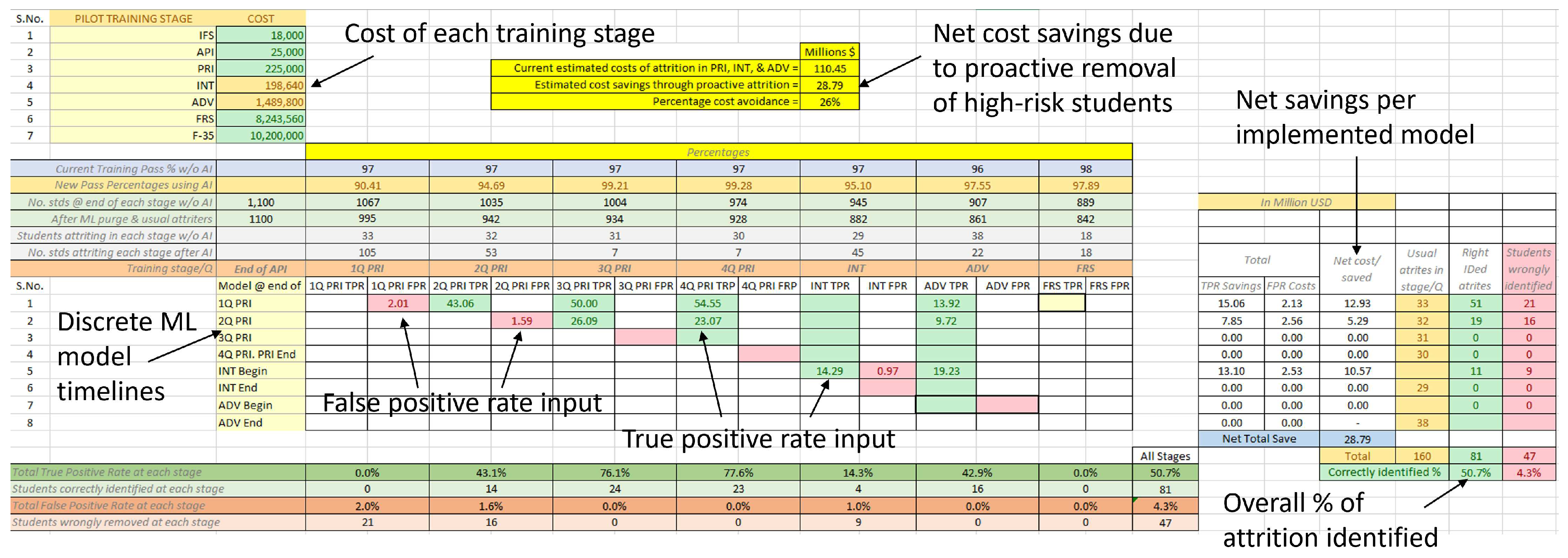
First, annual attrition costs to the U.S. Navy were estimated assuming 1,100 students in training, which is approximately the annual throughput of the U.S. Navy’s pilot training. Different aircraft (F-35, F-18, P3-P8, tilt rotors, and others) cost different total amounts to be trained on. The average cost to train aviators in different pipelines (including FRS stage) was estimated to be $6M. The cost of intermediate and advanced training was approximated accordingly. The attrition costs were then estimated as approximately $100 M per year using the observed attrition rates in primary (by quarter), intermediate, and advanced training stages.
Potential cost savings to the U.S. Navy were estimated by utilizing machine-learning models’ true positive and false positive performance metrics for each primary quarter, intermediate, and advanced stage. For example, if the end of primary stage attrition was predicted at the end of the first quarter of primary training, the direct cost savings are equal to the cost of providing training to a student aviator in the second, third, and fourth quarters of the primary stage. Each primary stage quarter was assumed to require an equal amount of resources. Assuming equal cost provides a conservative cost savings estimate as, in reality, later parts of primary training require more flight hours than earlier parts. For intermediate and advanced stages, the exact information on when a student aviator left the training program is not available and is assumed to be at the end of those stages. An Excel-based cost savings calculator was developed where a machine-learning model’s performance metrics can be input. This sheet calculates the cost savings due to true positive predictions, added costs due to false positives, and the net cost benefit or loss. Using this tool, at each decision point in time, the model with the best performance metrics and hence the most cost-benefit, if any, is chosen as the best one. After all such models’ results are entered, the cost savings per training stage as well as net value are calculated.
4. Results & Discussion
This section presents and discusses the results for both attrition prediction and pipeline suitability prediction. It then presents cost savings estimates resulting from pro-actively removing high-attrition risk students.
4.1. Attrition Prediction Results
Results are generated to demonstrate the feasibility of identifying likely unsuccessful student aviators using the proposed approach at different stages of training. Performance metrics for different machine-learning models utilizing only Q-1 primary stage flight grades data to predict attrition in Q-2, Q-3, or Q-4, on test data, is shown in Table 2. For instance, the gradient boosting model (GradBoost) has a false positive rate of 1.08% and true positive rates of 27.63%, 35.29%, and 43.75% for Q-2, Q-3, and Q-4, respectively. The model correctly identified 25 out of 66 flying-related attrition and 5 out of 23 DORs that occurred in those 3 quarters. Evaluation metrics MCC, F1, and AUROC, were respectively 0.41, 0.42, and 0.87.
The Receiver Operator Characteristic (ROC) curves for four models selected from the above table are shown in Figure 11.
Similarly different machine-learning models are evaluated to identify students that experienced attrition in either the intermediate or advanced stage after successfully completing primary training. ROC curves for different models are shown in Figure 12. Again, XG Boost models seem to perform the best with an AUROC value of 0.92. Further, the weight hyper-parameter given to the positive class labels (attrition class) in the XG Boost model was tuned by varying it to determine the most optimal value. Results showed that a value between 1 and 25 led to improved AUROC values. For each positive or negative prediction, the probability of a positive prediction can also be simultaneously generated.
Feature importance ranks, as generated by random forest models, are shown in Figure 14. The top 10 features that contribute the most to identifying attrition in the intermediate or advanced stage are depicted.
4.2. Pipeline Recommender Model Results
A number of models were trained to identify successful student aviators, at the end of primary training, who would be successful in the strike pipeline. The performance of those models against different performance metrics is summarized in Table 3. In addition, the ROC curves for the XG Boost, logistic regression, random forest, and LGBM models are provided in Figure 15. Figure 16 shows the normalized count of students according to their predicted strike-pipeline suitability scores (probability) compared to their target labels. The large distance between the two populations in the figure indicates that the models are performing well. It is important to note here that even the best-performing models classified some non-strike pipeline students as suitable for it. Some of these predictions may be due to the students’ preferences or the unavailability of strike pipeline slots during their transition to intermediate or advanced training. The others may be due to improper assignments that are expected to increase attrition rates in the later stages.
Similar to the attrition models, the top 10 features utilized by random forest models to classify a suitable strike pipeline student from others were identified. They are represented in Figure 17. These features could help guide instructors to concentrate on more important flight skills for students in primary training.
4.3. Potential Cost Savings Estimation
Potential cost savings through proactive removal of high attrition-risk students are estimated using the tool described in Section 3.4. After testing different models, the estimations shown are made using the models that give the most cost-benefit at each decision stage. It was observed that only models at three different instances during training resulted in cost savings being greater than additional costs due to false positive removals. The three models include one at end of Q-1, one at the end of Q-2, and the last one run at the beginning of intermediate training, which also included the training pipeline information. The false positive and true positive rates for different future training stages for these three models are shown in Figure 18. For example, the end of Q-1 model wrongly classified 2% of its active student population as having a high risk of attrition. This same model identified 43%, 50%, and 55% of those that experienced attrition during the second, third, and fourth quarters of primary training, respectively. It also identified 14% of students that experienced attrition in the advanced training.
Utilizing these three models, the estimated potential cost savings to the U.S. Navy was $29M per year, which corresponded to a 26% reduction in attrition costs. This assumed 1,100 student aviators at the beginning of primary training and using strike pipeline training costs. Considering other aircraft pipelines and lower average costs, the savings could still be nearly $20M per year. Results are indicated in Figure 19, which also shows True Positive Rate (TPR) savings, False Positive Rate (FPR) costs, and net benefit for each utilized model. The number of correctly identified and wrongly identified students is also reported for the test dataset. Overall, out of 160 students that experienced attrition in all the considered training stages, 81 (51%) were correctly identified and 47 (4%) would have been wrongly eliminated from training. It is important to note here that instructor-given grades and attrition decisions include human subjectivity, which make highly-accurate classification of students impossible. Also, the objective is not to identify all the students that would experience attrition, but to closely quantify the risk of attrition, which then can guide decision makers to make such decisions.
5. Conclusions & Future Work
This work demonstrated the feasibility of extracting useful features from primary training flight item grades and applying machine-learning techniques to identify U.S. naval student aviators with a high risk of attrition in primary, intermediate, and advanced stages of training. Using historical data, 50% of those that experienced attrition in later stages were identified with only 4% false positive rate. These results indicate that a 26% reduction in attrition costs for the U.S. Navy could be achieved by implementing a policy of proactive removal of all students identified to experience attrition. Alternatively, only students with very high attrition risk could be removed, while those with moderate risk could be provided with additional resources to improve their chances. These results could be further improved by incorporating additional information such as primary stage academic grades, students’ pipeline preferences, pipeline slots availability, intermediate and advanced stage flight, and academic grades, and by optimizing the hyper-parameters of the machine-learning models considered. Also, each machine-learning prediction could be supplemented by explanations [24] that can aid in implementing student-customized training activities.
In addition to attrition prediction, trained machine-learning models were demonstrated to successfully identify student aviators suitable for the strike pipeline. This could be similarly achieved for other pipelines. Students could be rank-ordered according to their probabilities of success, as provided by the machine-learning models. These ranks could help allocate students, especially when training slots are limited for one or more pipelines. Automated pipeline recommendations and rankings could help reduce the burden on flight instructors and reduce mismatches. This would further reduce attrition rates in intermediate and advanced training. These recommendations would also be beneficial when a student aviator chooses, or is required, to change pipelines during intermediate or advanced training.
This research demonstrated the strong potential and benefits of implementing data-driven techniques such as the ones discussed herein to improve U.S. naval pilot training operations. However, thorough testing and shadow real-time implementation may be needed before actively deploying and trusting their results.
Author Contributions
Conceptualization, J.P., N.R., and T.P.; methodology, J.P., O.F., and J.W; software, J.P.; validation, J.P., O.F., and J.W.; formal analysis, J.P. and J.W.; investigation, J.P.; resources, M.N., M.T., and B.A; data curation, M.N., M.T., and B.A.; writing—original draft preparation, J.P.; writing—review and editing, J.P., O.F., and N.R.; visualization, J.P. and O.F.; supervision, J.W. and D.M.; project administration, J.W. and D.M.; funding acquisition, J.P., J.W., M.N., M.T., and B.A. All authors have read and agreed to the published version of the manuscript.
Funding
This research was partially funded by the U.S. Naval Air Systems Command (NAVAIR), Contract Number N68335-21-C-0865.
Data Availability Statement
Data pertaining to the results is contained within the article. Restrictions apply to the availability of the data, utilized to extract features and train the machine-learning models, which were provided by the U.S. Navy.
Acknowledgments
The authors would like to thank Mr. Roger Jacobs for providing subject matter expertise during this project.
Conflicts of Interest
This study was conducted under a STTR grant to Global Technology Connection, Inc., and was funded by the U.S. Naval Air Systems Command.
Abbreviations
The following abbreviations are used in this manuscript:
| ADV | Advanced Training Stage |
| AUROC | Area Under the Receiver Operating Characteristic Curve |
| API | Aviation Preflight Indoctrination |
| ASTB | Aviation Selection Test Battery |
| CNATRA | Chief of Naval Air Training |
| DOR | Drop On Request |
| FNR | False Negative Rate |
| FPR | False Positive Rate |
| FRS | Fleet Replacement Squadron |
| IFS | Initial Flight School |
| INT | Intermediate Training Stage |
| MIF | Maneuver Item File |
| MCC | Matthews Correlation Coefficient |
| MLP | Multi-Layer Perceptron |
| NIFE | Naval Introductory Flight Evaluation |
| NSS | Naval Standardized Scores |
| PRI | Primary Training Stage |
| ROC | Receiver Operator Characteristic |
| SNA | Student Naval Aviators |
| SNFO | Student Naval Flight Officers |
| SVM | Support Vector Machine |
| TNR | True Negative Rate |
| TPR | True Positive Rate |
References
- Arnold, R.D.; Phillips, J.B. Causes of student attrition in US naval aviation training: A five year review from FY 2003 to FY 2007. Technical report, NAVAL AEROSPACE MEDICAL RESEARCH LAB PENSACOLA FL, 2008.
- Kamel, M.N. Employing Machine Learning to Predict Student Aviator Performance. Technical report, NAVAL POSTGRADUATE SCHOOL MONTEREY CA MONTEREY United States, 2020.
- Erjavec, S.J. ESTIMATING THE PROBABILITY THAT NAVAL FLIGHT STUDENTS WILL PASS PRIMARY FLIGHT TRAINING AT THREE KEY MILESTONES. PhD thesis, Monterey, CA; Naval Postgraduate School, 2019.
- Mattock, M.G.; Asch, B.J.; Hosek, J.; Boito, M. The relative cost-effectiveness of retaining versus accessing Air Force pilots. Technical report, RAND Corporation Santa Monica United States, 2019.
- Report to Congressional Armed Services Committees on Initiatives for Mitigating Military Pilot Shortfalls, 2019. https://prhome.defense.gov/Portals/52/Documents/Report%20to%20Congress%20on%20Initiatives%20for%20Mitigating%20Military%20Pilot%20Shortfalls%20cleared%20for%20public%20release.pdf.
- Griffin, G.; McBride, D. Multitask Performance: Predicting Success in Naval Aviation Primary Flight Training. Technical report, NAVAL AEROSPACE MEDICAL RESEARCH LAB PENSACOLA FL, 1986.
- Delaney, H.D. Dichotic listening and psychomotor task performance as predictors of naval primary flight-training criteria. The International Journal of Aviation Psychology 1992, 2, 107–120. [CrossRef]
- Carretta, T.R.; Ree, M.J. Air Force Officer Qualifying Test validity for predicting pilot training performance. Journal of Business and Psychology 1995, 9, 379–388. [CrossRef]
- Burke, E.; Hobson, C.; Linsky, C. Large sample validations of three general predictors of pilot training success. The International journal of aviation psychology 1997, 7, 225–234. [CrossRef]
- Hormann, H.J.; Maschke, P. On the relation between personality and job performance of airline pilots. The International Journal of Aviation Psychology 1996, 6, 171–178. [CrossRef]
- Bair, J.T.; Lockman, R.F.; Martoccia, C.T. Validity and factor analyses of naval air training predictor and criterion measurers. Journal of Applied Psychology 1956, 40, 213. [CrossRef]
- Rowe, N.C.; Das, A. Predicting success in training of Navy aviators. International Command and Control Research and Technology Symposium (ICCRTS), 2021. https://faculty.nps.edu/ncrowe/oldstudents/ICCRTS_aviator_training_ncrowe_21.htm.
- Street Jr, D.; Helton, K.; Dolgin, D. The unique contribution of selected personality tests to the prediction of success in naval pilot training. Technical report, NAVAL AEROSPACE MEDICAL RESEARCH LAB PENSACOLA FL, 1992.
- Bale, R.M.; Rickus, G.M.; Ambler, R.K. Prediction of advanced level aviation performance criteria from early training and selection variables. Journal of Applied Psychology 1973, 58, 347. [CrossRef]
- Hunter, D.R.; Burke, E.F. Meta analysis of aircraft pilot selection measures. Technical report, ARMY RESEARCH INST FOR THE BEHAVIORAL AND SOCIAL SCIENCES ALEXANDRIA VA, 1992.
- Caraway, C.L. A looming pilot shortage: It is time to revisit regulations. International Journal of Aviation, Aeronautics, and Aerospace 2020, 7, 3. [CrossRef]
- New Naval Introductory Flight Evaluation Program Provides Modern Foundation for Flight Tr.
- Jenkins, P.R.; Caballero, W.N.; Hill, R.R. Predicting success in United States Air Force pilot training using machine learning techniques. Socio-Economic Planning Sciences 2022, 79, 101121. [CrossRef]
- Akers, C.M. Undergraduate Pilot Training Attrition: An Analysis of Individual and Class Composition Component Factors 2020.
- Rowe, N.C. Automated Trend Analysis for Navy-Carrier Landing Attempts. Interservice/Industry Training, Simulation, and Education Conference (I/ITSEC), 2012. https://faculty.nps.edu/ncrowe/rowe_itsec12_paper12247.htm.
- Phillips, J.; Chernyshenko, O.; Stark, S.; Drasgow, F.; Phillips, I.; others. Development of scoring procedures for the Performance Based Measurement (PBM) test: Psychometric and criterion validity investigation. Technical report, NAVAL MEDICAL RESEARCH UNIT DAYTON WRIGHT-PATTERSON AFB OH, 2011.
- He, H.; Bai, Y.; Garcia, E.A.; Li, S. ADASYN: Adaptive synthetic sampling approach for imbalanced learning. 2008 IEEE international joint conference on neural networks (IEEE world congress on computational intelligence). IEEE, 2008, pp. 1322–1328.
- Mishra, S. Handling imbalanced data: SMOTE vs. random undersampling. Int. Res. J. Eng. Technol 2017, 4, 317–320.
- Lundberg, S.M.; Lee, S.I. A unified approach to interpreting model predictions. Advances in neural information processing systems 2017, 30.
Figure 1.
CNATRA’s six student navy aviator training pipelines [2].
Figure 1.
CNATRA’s six student navy aviator training pipelines [2].
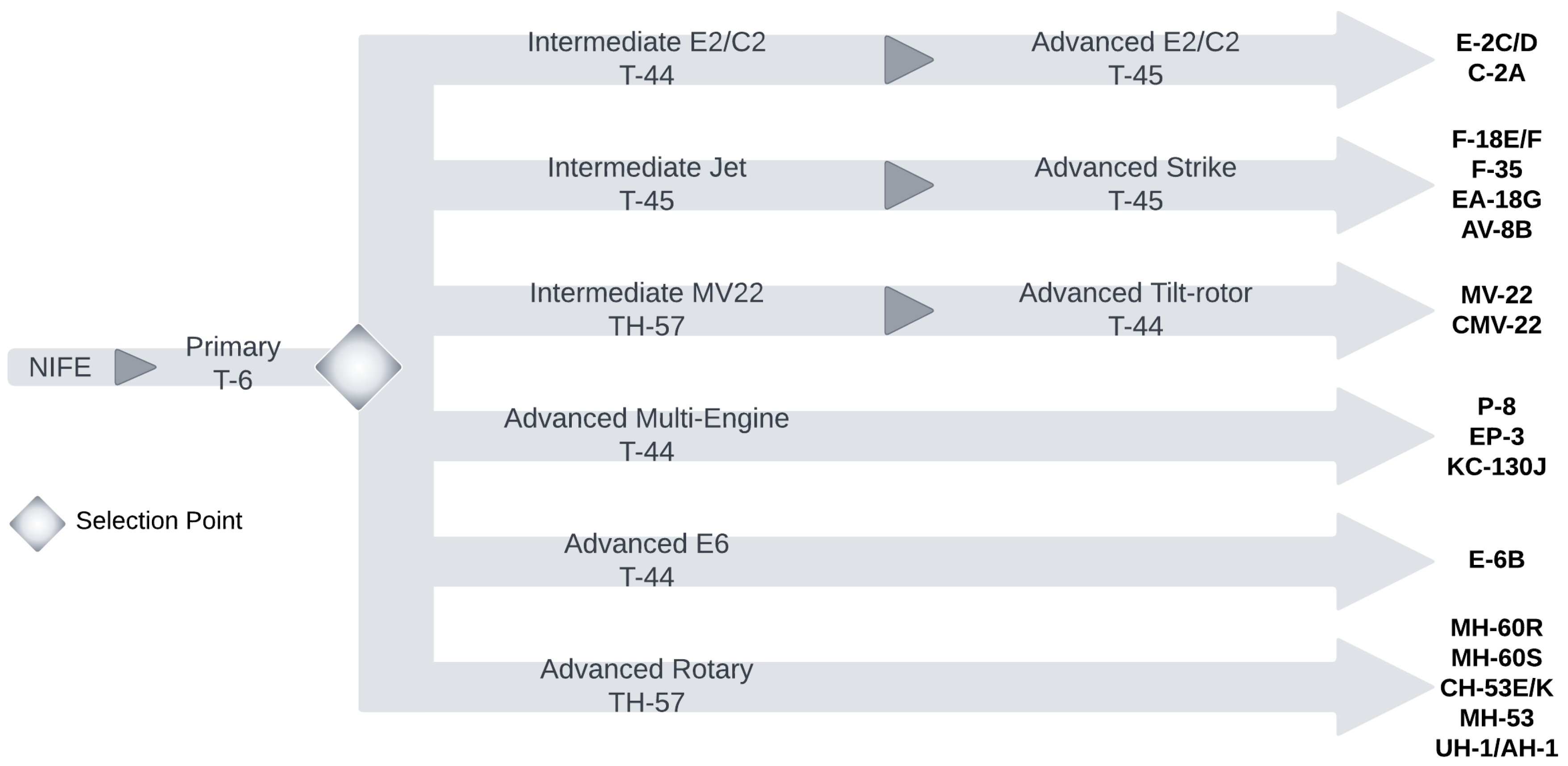
Figure 2.
Distribution of student attrition, by reason for attrition, during (a) Primary, (b) Intermediate, and (c) Advanced training stages.
Figure 2.
Distribution of student attrition, by reason for attrition, during (a) Primary, (b) Intermediate, and (c) Advanced training stages.
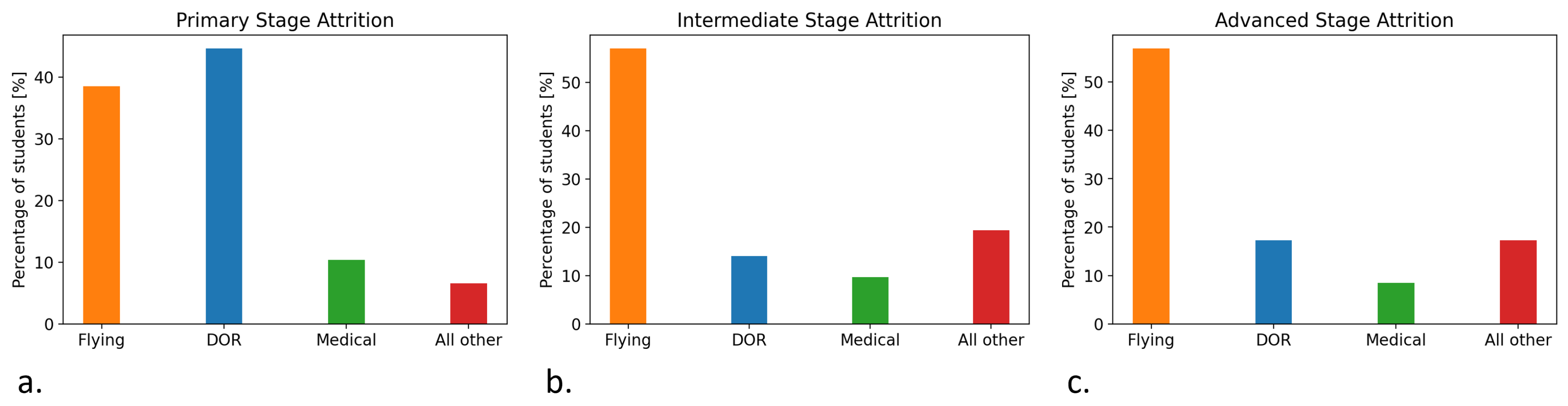
Figure 3.
Left: Reason for primary stage attrition by quarter; Right: Distribution of primary stage attrition cost by reason for attrition.
Figure 3.
Left: Reason for primary stage attrition by quarter; Right: Distribution of primary stage attrition cost by reason for attrition.
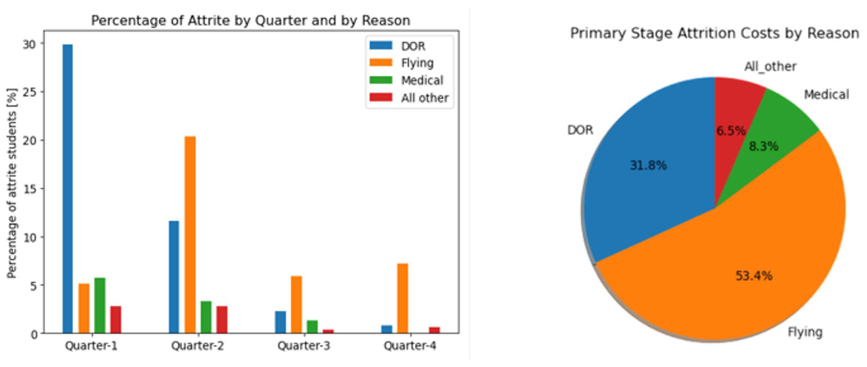
Figure 4.
Naval student aviator attrition rates and associated cumulative attrition costs for the strike pipeline at different stages of training.
Figure 4.
Naval student aviator attrition rates and associated cumulative attrition costs for the strike pipeline at different stages of training.
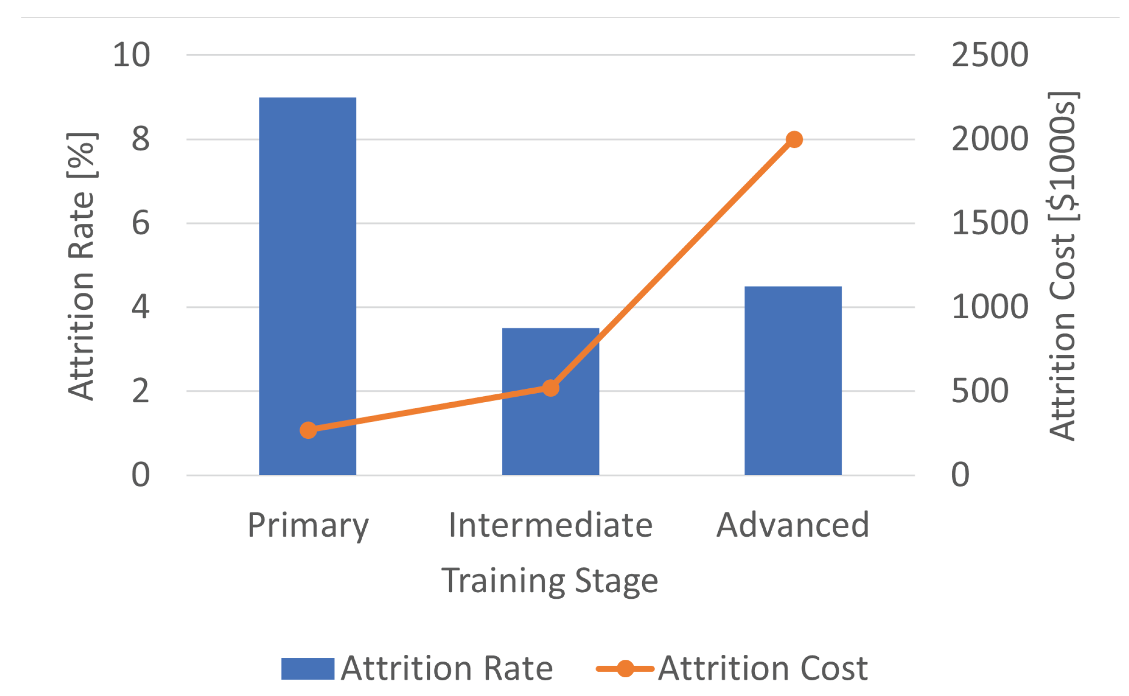
Figure 5.
Overview of datasets used for the purpose of this research.
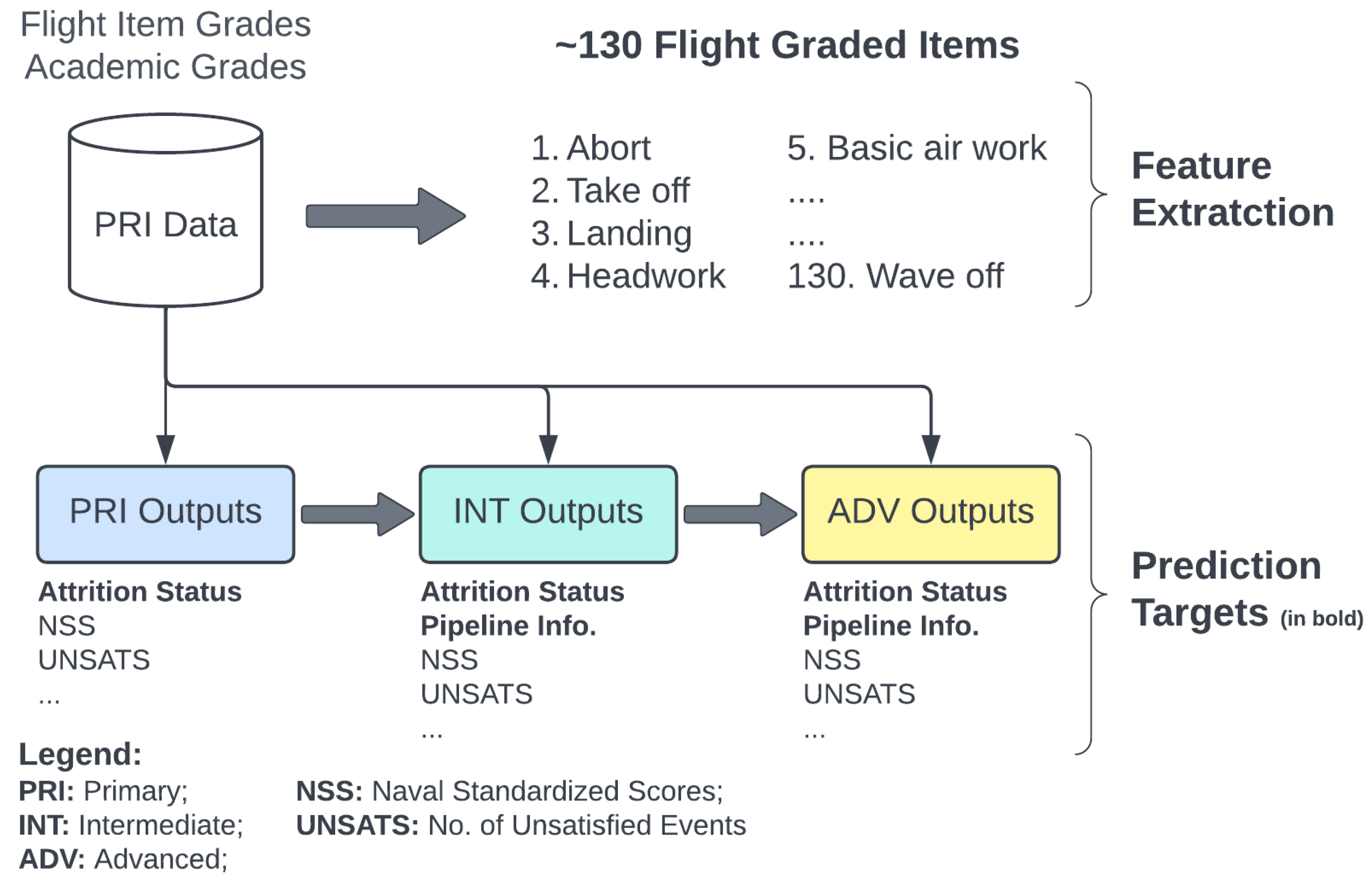
Figure 6.
Venn diagram of number of students’ data available in cumulative outcome tables.
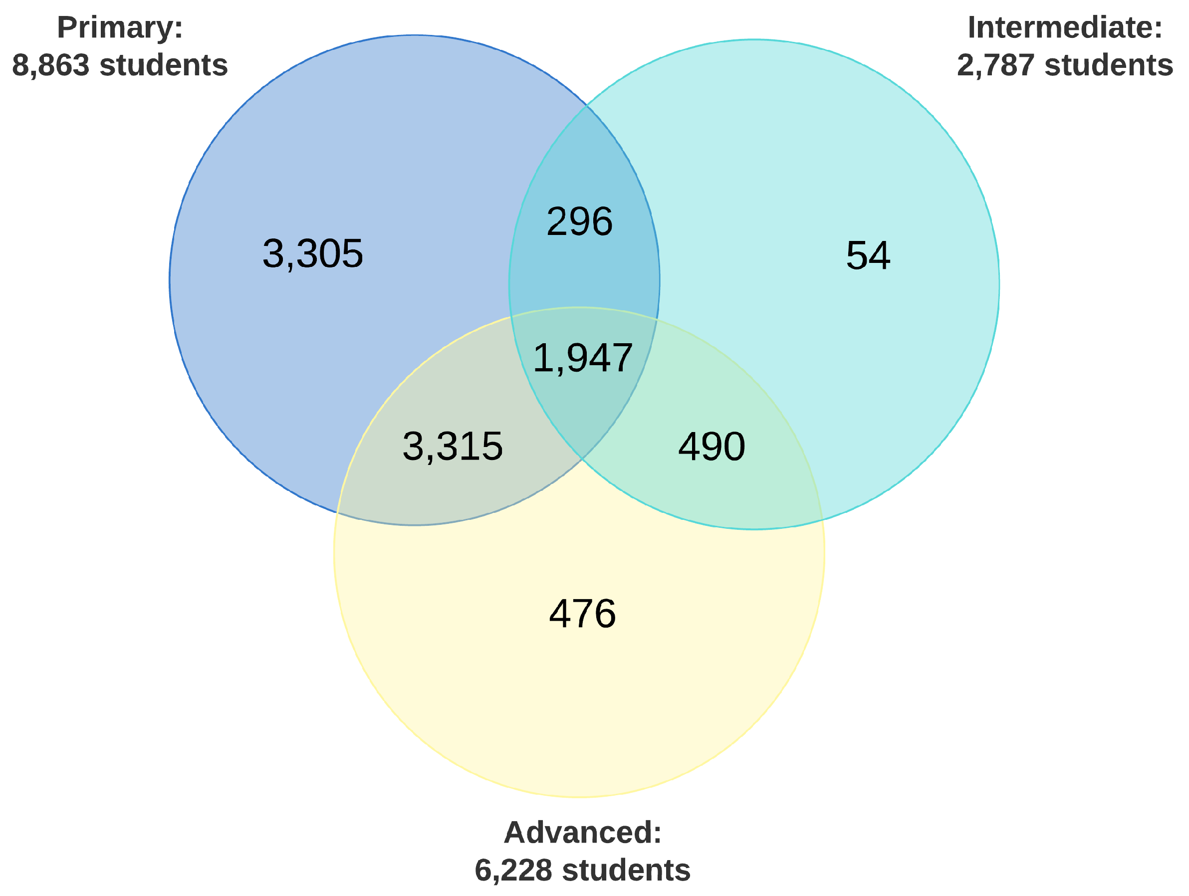
Figure 7.
Prediction targets and SME guided features extracted from flight graded items.
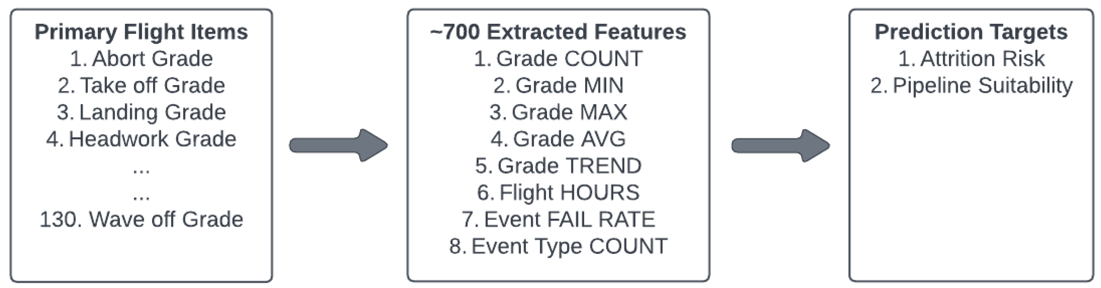
Figure 8.
Qualitative depiction of reduction in data sparsity through aggregation and feature extraction. White spaces indicate empty cells.
Figure 8.
Qualitative depiction of reduction in data sparsity through aggregation and feature extraction. White spaces indicate empty cells.
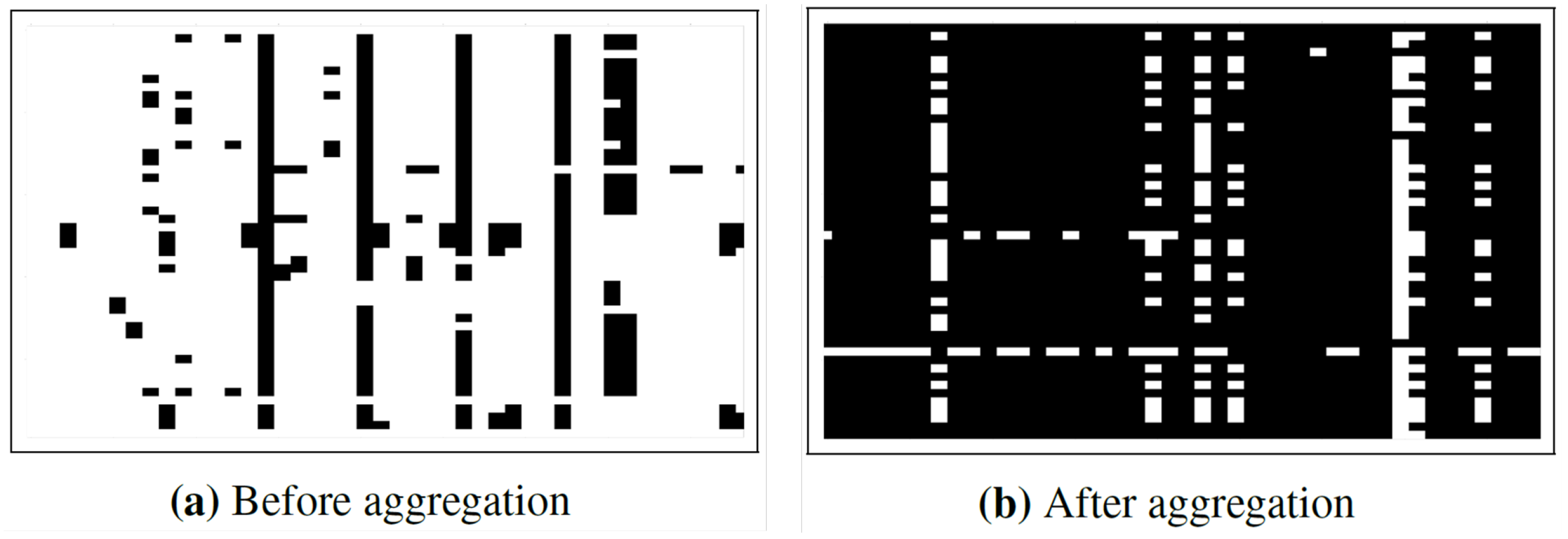
Figure 9.
Depiction of the different machine-learning models and when they would be leveraged.
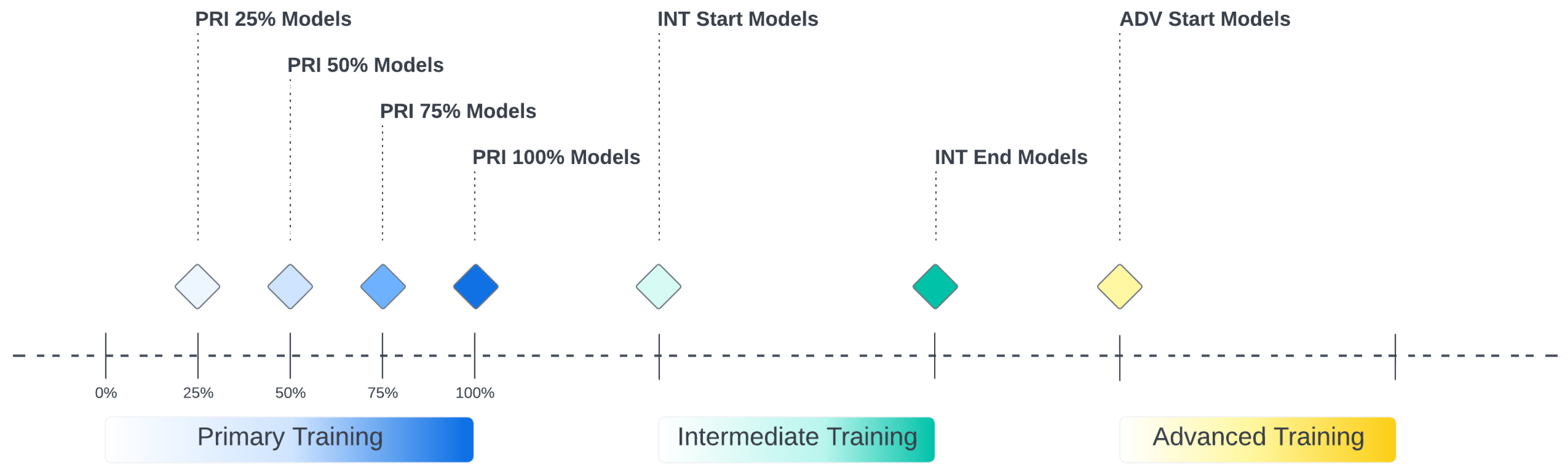
Figure 11.
Performance of different machine-learning models in identifying primary stage attrition.
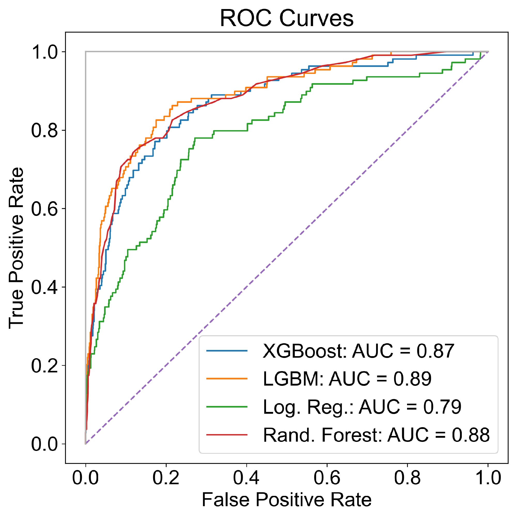
Figure 12.
Performance of different machine-learning models to identify students that experienced attrition in intermediate or advanced stage.
Figure 12.
Performance of different machine-learning models to identify students that experienced attrition in intermediate or advanced stage.
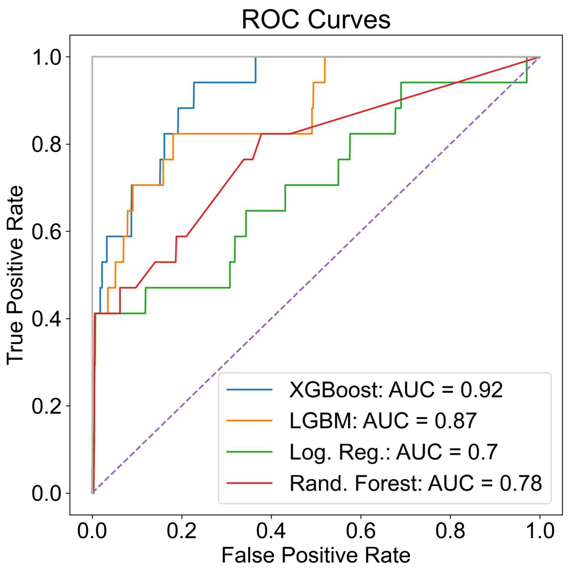
Figure 13.
Effect of positive class weights.
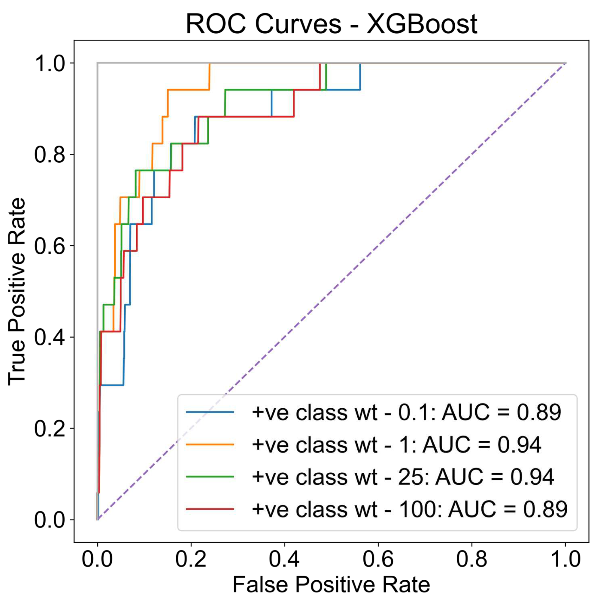
Figure 14.
Top 10 features utilized to estimate attrition risk.
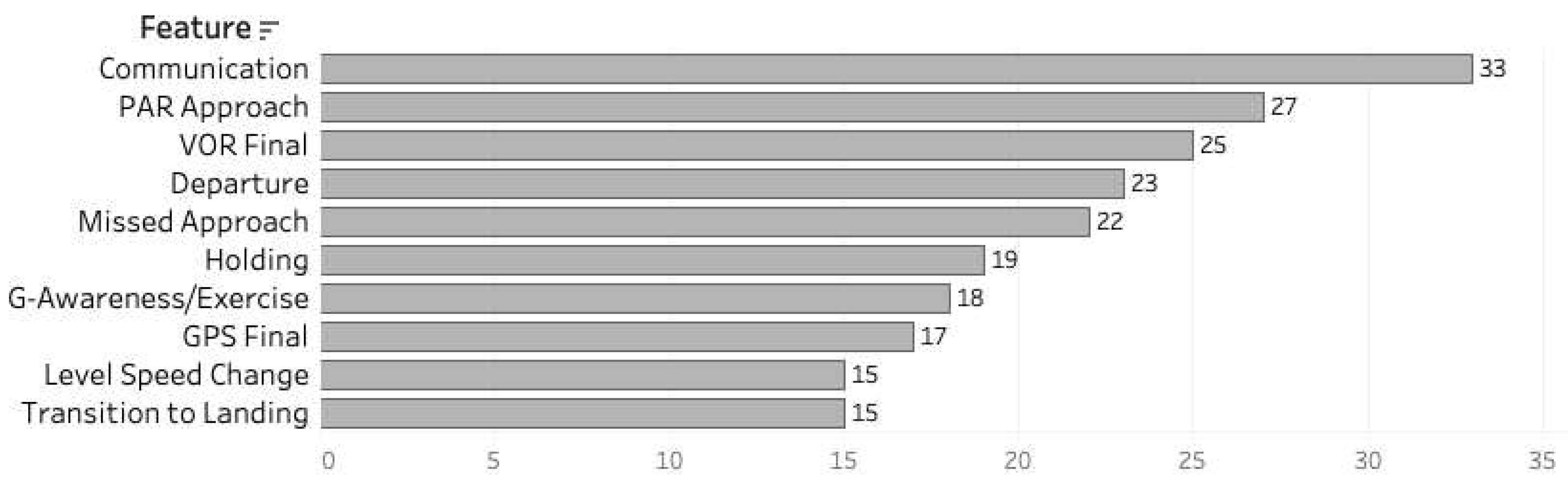
Figure 15.
AUROC of Pipeline suitability model.
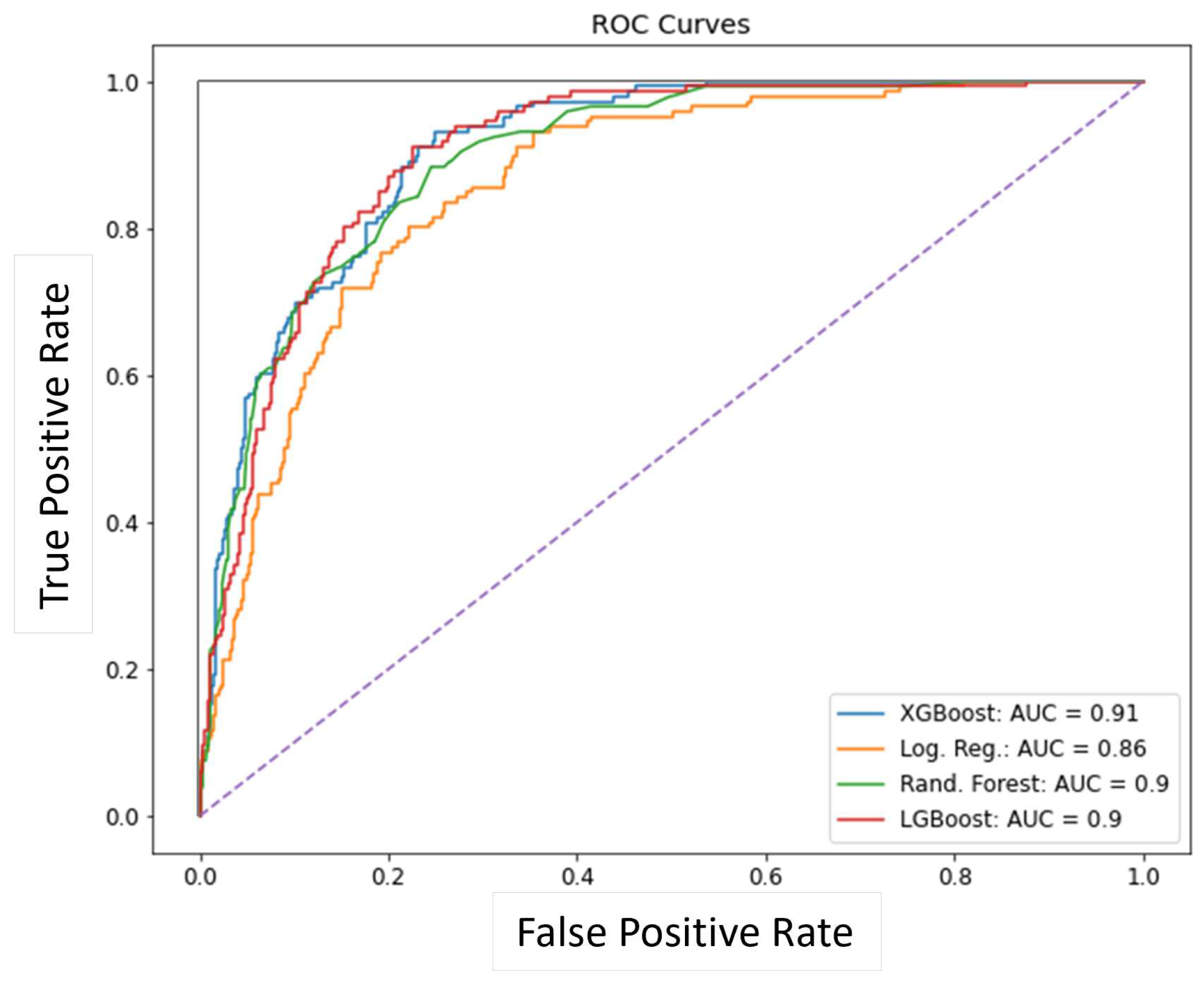
Figure 16.
Pipeline probability score.
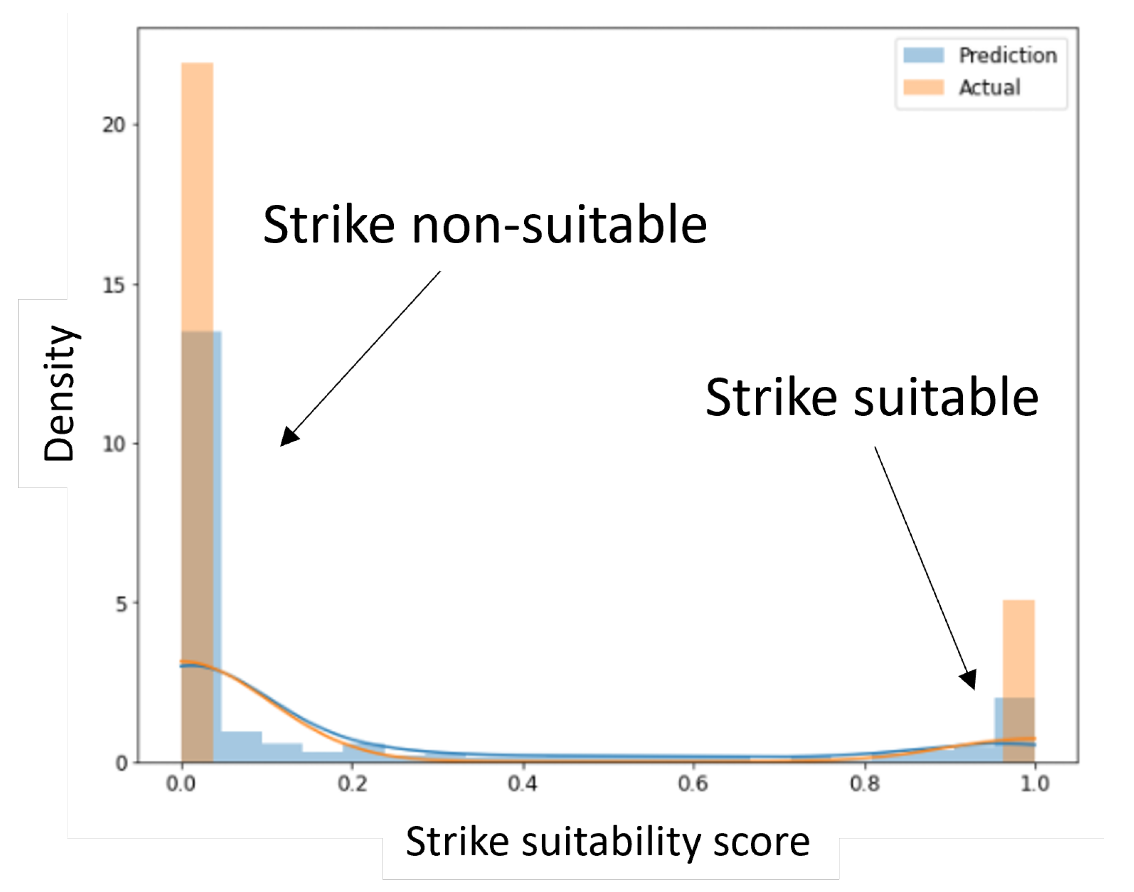
Figure 17.
Top 10 features to identify successful strike students.
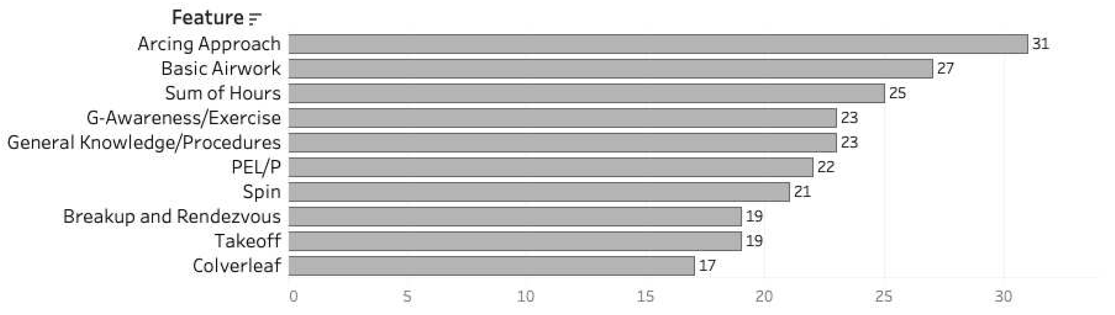
Figure 18.
True and false positive rate of selected ML models for the most cost benefit.
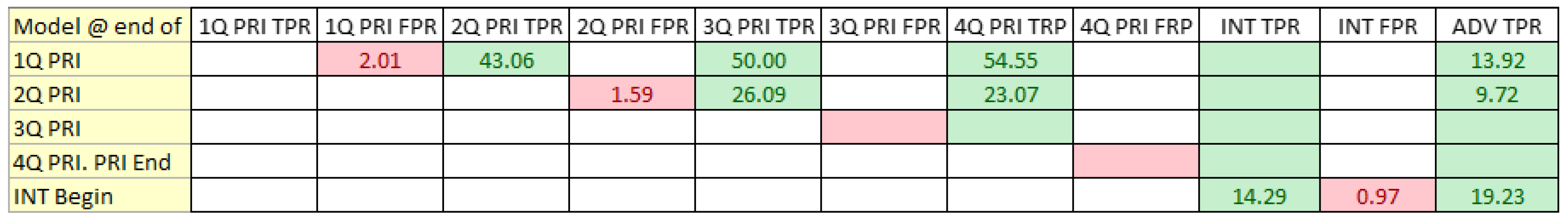
Figure 19.
Cost savings generated and classification results produced by each selected model and net potential cost savings.
Figure 19.
Cost savings generated and classification results produced by each selected model and net potential cost savings.
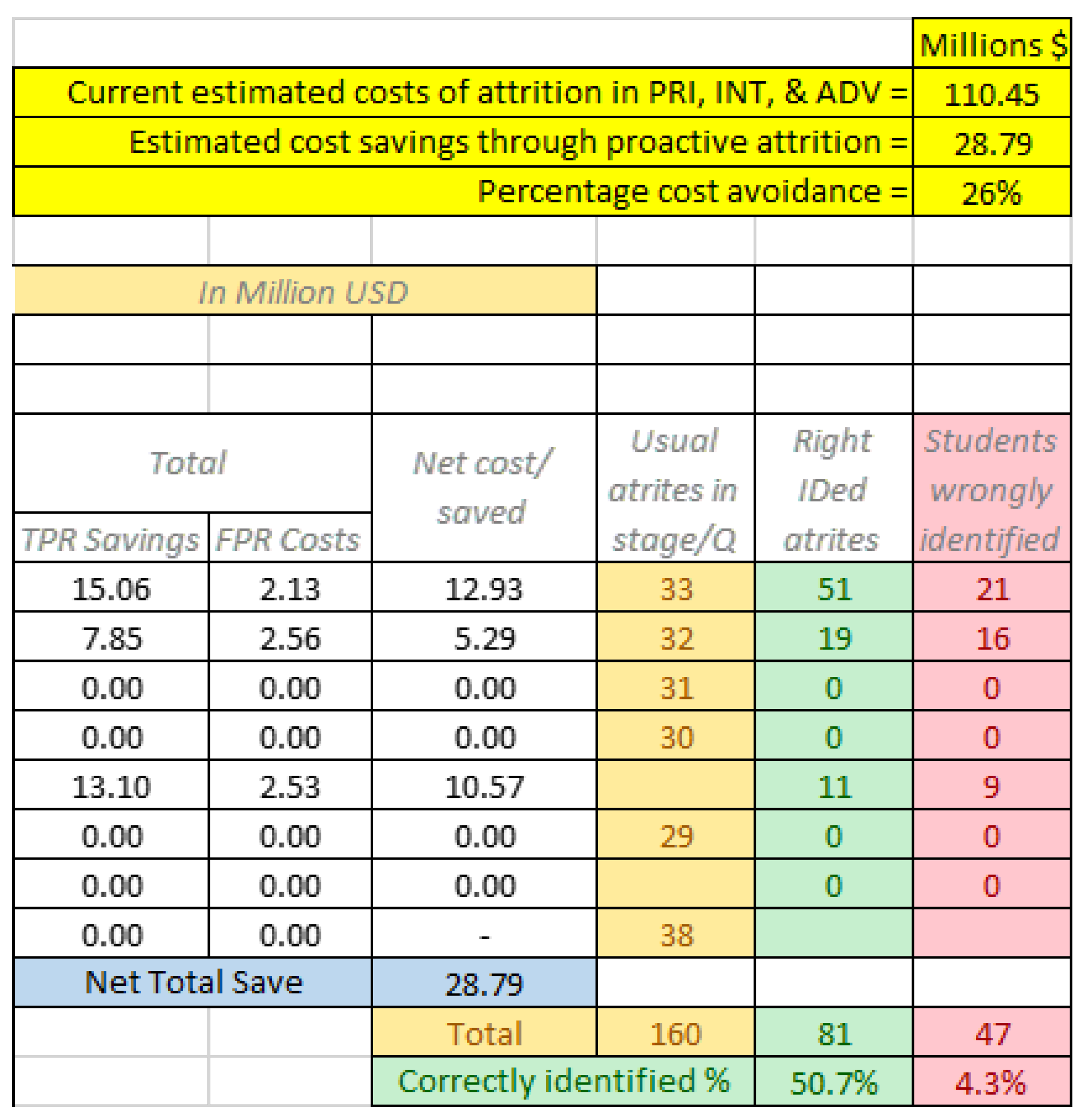

Table 1.
Data available at different stages of training and ML models used.
| S. No | Timeline | PRI Grades | PRI Syllabus | PRI Outcome | INT Syllabus | INT Outcome | ADV Syllabus | Targets |
|---|---|---|---|---|---|---|---|---|
| 1 | During PRI | Yes | Yes | Attrition Risk, Pipeline Suitability | ||||
| 2 | End of PRI | Yes | Yes | Yes | Attrition Risk, Pipeline Suitability | |||
| 3 | During INT | Yes | Yes | Yes | Yes | Attrition Risk Predictor | ||
| 4 | End of INT | Yes | Yes | Yes | Yes | Yes | Attrition Risk Predictor | |
| 5 | During ADV | Yes | Yes | Yes | Yes | Yes | Yes | Attrition Risk Predictor |
Table 2.
Performance of ML models identifying primary stage attrition using PRI Q-1 data.
| Model | FPR (%) | Q2 TPR (%) | Q3 TPR (%) | Q4 TPR (%) | Flight Attr. Id’ed | DOR Attr. Id’ed | MCC | F1 | AUROC |
|---|---|---|---|---|---|---|---|---|---|
| Ad BagOS | 5.35 | 36.84 | 35.29 | 37.50 | 26/66 | 8/23 | 0.31 | 0.36 | 0.83 |
| XG Boost | 1.08 | 36.84 | 41.18 | 62.5 | 33/66 | 7/23 | 0.51 | 0.52 | 0.87 |
| Log Reg | 5.52 | 39.47 | 35.29 | 43.758 | 27/66 | 7/23 | 0.29 | 0.35 | 0.79 |
| RF | 1.02 | 22.37 | 41.18 | 43.75 | 23/66 | 4/23 | 0.39 | 0.39 | 0.87 |
| Grad Boost | 1.08 | 27.63 | 35.29 | 43.75 | 25/66 | 5/23 | 0.41 | 0.42 | 0.87 |
| LGBM | 0.80 | 22.37 | 41.18 | 31.25 | 23/66 | 5/23 | 0.39 | 0.38 | 0.89 |
| MLP | 3.19 | 35.53 | 23.53 | 43.75 | 27/66 | 6/23 | 0.32 | 0.37 | 0.79 |
Table 3.
ML models performance in estimating strike pipeline suitability .
| S. No | Model | TPR (%) | FNR (%) | TNR (%) | FPR (%) | MCC | F1 | Recall | Precision | Accuracy | AUROC |
|---|---|---|---|---|---|---|---|---|---|---|---|
| 0 | RF | 85.80 | 14.20 | 81.53 | 18.47 | 57.94 | 66.34 | 85.80 | 54.08 | 82.40 | 91.20 |
| 1 | AdBoost | 86.44 | 13.56 | 82.17 | 17.83 | 59.22 | 67.32 | 86.44 | 55.13 | 83.04 | 91.42 |
| 2 | XG Boost | 78.23 | 21.77 | 89.61 | 10.39 | 63.70 | 71.37 | 78.23 | 65.61 | 87.31 | 91.32 |
| 3 | LGBM | 80.76 | 19.24 | 87.21 | 12.79 | 61.83 | 69.85 | 80.76 | 61.54 | 85.91 | 91.49 |
Disclaimer/Publisher’s Note: The statements, opinions and data contained in all publications are solely those of the individual author(s) and contributor(s) and not of MDPI and/or the editor(s). MDPI and/or the editor(s) disclaim responsibility for any injury to people or property resulting from any ideas, methods, instructions or products referred to in the content. |
© 2023 by the authors. Licensee MDPI, Basel, Switzerland. This article is an open access article distributed under the terms and conditions of the Creative Commons Attribution (CC BY) license (http://creativecommons.org/licenses/by/4.0/).
Copyright: This open access article is published under a Creative Commons CC BY 4.0 license, which permit the free download, distribution, and reuse, provided that the author and preprint are cited in any reuse.


