
Submitted:
22 February 2023
Posted:
23 February 2023
You are already at the latest version
Abstract
Deep learning has already revolutionised the way we process a wide range of data, in many areas of our daily life. The ability to learn abstractions and relationships from heterogeneous data, has provided impressively accurate prediction and classification tools to handle increasingly big datasets. This has a significant impact on the growing wealth of omics datasets, with the unprecedented opportunity for a better understanding of the complexity of living organisms. While this revolution is transforming the way we analyse these data, explainable deep learning is emerging as an additional tool with the potential to change the way we interpret biological data. Explainability addresses critical issues such as transparency, so important when computational tools are introduced especially in clinical environments. Moreover, it empowers artificial intelligence with the capability to provide new insights in the input data, thus adding an element of discovery to these already powerful resources. In this review we provide an overview of the transformative effects explainable deep learning is having on multiple sectors, ranging from genome engineering and genomics, from radiomics to drug design and clinical trials. We offer a perspective to life scientists, to better understand the potential of these tools, and a motivation to implement them in their research, by suggesting learning resources they can use to move their first steps in this field.
Keywords:
Explainability
; Deep Learning
; Artificial Intelligence
; Genomics
; Transcriptomics
Introduction
The concept of artificial intelligence (AI) dates back to the half of the twentieth century, and refers to the development of computer systems capable of performing tasks with a level of complexity comparable to Human intelligence. There is not an agreed and standard definition of AI, as much as the concept of intelligence itself remains rather blurry, and depends on the context. In a biological and medical context, one might describe artificial intelligence as a system that is capable of interpreting external data in a meaningful way, to learn new information from them, and to use that learning process in order to draw conclusions and adapt [1,2]. In other scenarios, the capability to draw conclusions, and therefore to automate decision processes, is probably a major feature in defining what AI is [3].
There are many reasons explaining why artificial intelligence has become a hot topic in many research fields, including biotechnology and life sciences. A key motivation is the increasing complexity and dimensionality of data, which are generated by increasingly accessible and cheaper technologies. This phenomenon has contributed to “big-data” becoming another critical aspect of modern life sciences. Big data refers to some of the characteristics of the datasets these new technologies can generate, such as:
- -
- storage footprint: the raw data, the intermediate analysis files and the results of their analysis occupy increasingly more disk space (i.e. the raw sequence of a Human whole-genome might vary between 100GB to 150GB depending on the coverage);
- -
- number of data points: high-throughput technologies allow to process thousands of samples in a relatively short time, thus multiplying the number of data points collected during each experiment; this further increases when single-cell technologies are employed [4];
- -
- range of data types: genomic, epigenetic, transcriptomic, proteomic data - among others - can be generated from each single sample, with the intent of combining their information for the analysis [5].
Given the availability of these technologies at reasonable prices per sample, the generation of an increasing wealth of data shifts the real challenge to the dimensionality of the datasets. When we use the term “dimensionality” we refer to the number of variables (or features) describing each record in a dataset. This problem has been known for many years and regarded as the “curse of dimensionality”: it refers to the difficulty to represent or uncover the relationships between variables when the number of variables (i.e. dimensions) per data point increases. Especially in biology and life sciences, the increase in dimensionality corresponds to the higher number of descriptors necessary to characterise more complex phenomena, which in turn represents an obstacle in identifying meaningful trends or patterns in the data.
Additionally, the accessibility of -omics technologies offers an unprecedented opportunity to measure biological phenomena using multiple data sources, which can be integrated with each other: the need for data integration, however, further increases the computational and statistical challenges associated with handling big data [5,6].
Finally, larger datasets require an additional effort in terms of data quality since the noise and potential bias impacting the analysis might increase with dimensionality, and might have a significant impact on the results.
In this scenario, it is evident that extracting meaningful knowledge from increasingly complex data remains a major issue in bioinformatics. This is the reason why emerging artificial intelligence applications have offered new opportunities in the analysis of omics data. AI plays a critical role in allowing big datasets to be tractable. And among artificial intelligence approaches, deep learning (DL) provides extremely valuable solutions. In fact, while machine learning and deep learning share some learning properties of their algorithms, the way they handle the inputs is quite different. The main difference between the two is that machine learning often requires initial feature engineering [7]: the input data need to be manually transformed into a set of features and format that can be successfully processed by machine learning algorithms. Deep learning on the other hand can automatically learn multiple levels of abstraction and representations of the relationships between the features in the input dataset: this capability allows to skip manual feature engineering and facilitates the analysis of high dimensional and complex data without additional and potentially biassing steps [8]. Moreover, deep learning can provide additional help when dealing with heterogeneous data and in the data integration process.
These tools have therefore a huge potential to resolve unmet challenges, and the number of applications of deep learning to the analysis of omics data has exponentially increased during the past few years. For the scope of this review, we are particularly interested in a specific subset of these methods, i.e. explainable deep learning.
Explainability refers to the ability to provide an understandable explanation of a model’s predictions and decisions. For this reason, this area covers a large number of approaches significantly different in their goals. Here, we focus in particular on the so-called post-hoc explainability, i.e. methods aiming at explaining a deep learning model once it has been trained [9]. This is different from integrating interpretability features into the structure of the model. A post-hoc explainability approach can be used for three main objectives [10,11]:
- (a)
- Transparency and trust: machine learning and deep learning are considered “black boxes” and this rarely fits with contexts (healthcare, for example) where a justification should be provided for decisions. Explainability offers a solution, i.e. opens the black box and provides the means to connect the outcome of a model to the information it received as an input, or to reveal the inner mechanisms of the model, i.e. how a decision or a prediction has been reached.
- (b)
- Quality control or troubleshooting: mapping the outcomes of an artificial neural network to those features in the input which contributed most to the activation of the model, and therefore to reaching its decisions, helps identifying any bias in the datasets, and to spot input features which should not be expected to influence the model to a certain extent.
- (c)
- Novel insights: assigning an importance score to those input features that best contribute to the outcome of a deep neural network, provides a way to identify relationships in the data that other methods might not be able to reveal.
This last use of explainable AI is the most interesting for us: while supervised artificial intelligence has been successfully used to make predictions and classifications, explainability adds a third and equally important dimension to AI, i.e. new tools for discovery [11,12,13].
There is a wide range of methods available to provide post-hoc explainability to a deep learning model, reviewed extensively elsewhere [14]: of particular interest for this review, some are based on propagating the model activation backwards from the output to the input [15,16,17], or designed to assign a score to the relative contribution of an input feature to the outcome of the model [18], or to assign a similar score to the relationship between input features [19]. A schematic overview of a few selected categories of explainable methods is represented in Figure 1.
In this review we will focus on the role that explainable deep learning is having in providing novel insights, and we will highlight the impact this approach will have on a wide range of life science and omics data analyses.
Explainable DL and Genome Engineering
A variety of biotechnology settings, from healthcare improvement [20,21,22] to food production [23,24], leverage artificial intelligence [25]. Specifically, deep learning, originally inspired by biological models of computation and cognition in the human brain [26], is rapidly replacing traditional AI algorithms in numerous fields, including gene therapy [27,28,29,30], drug research [31], medical image analysis [32,33], and genetics [11,34]. The DL’s strength over other machine learning techniques, i.e. is its ability to detect and classify non-linear relationships in a dataset, is an invaluable asset in this area.
The clustered regularly interspaced short palindromic repeat (CRISPR)-based systems are among the most promising tools for genetic manipulation. The CRISPR toolbox and its applications have profoundly changed biological research, impacting agricultural practices and genomic medicine [35]. Notably, this technology has a significant potential in addressing genetically determined Human diseases, because genome editing provides the means to correct genetic variants and modify specific gene functions, thus offering actionability for otherwise incurable pathologies. One of the most critical aspects of designing CRISPR intervention though, is the ability to control on-target versus off-target mutations: the implications are evident when CRISPR is used to plan medical interventions and gene therapies on Human beings. In this field, deep learning shows tremendous potential to help predicting CRISPR outcomes, by integrating high-dimensional heterogeneous data, such as sequence composition and secondary structure, thermodynamics, and chromatin accessibility within cell-specific contexts. Convolutional neural networks (CNNs) are particularly attractive solutions for the design of sgRNAs and predicting genome editing outcomes: they are able to perform feature extraction directly from sequence data via one-hot encoding, and offer improved interpretability of the biological data compared to state-of-the-art methods.
A wide array of deep-learning methods has therefore been developed to address these very challenging and outcome-determining aspects of genome engineering. For example, Xue and colleagues [36] developed a CNN model to predict the sgRNA activity for the CRISPR-Cas9 system, from public experimentally validated sgRNA efficacy datasets in gene knockouts, covering several cell types, across five species. To capture the sgRNA motifs which determine the target activity of genome editing, a convolutional kernel visualisation strategy was implemented, assigning an importance score to nucleotide positions. A strong preference for guanine and a low preference for thymine were shown in different cell types. The nucleotide composition of the sgRNA seed region was then identified as the major driver for the formation of the guide-RNA-target-DNA heteroduplex. By deploying CNN coupled with explainability, the authors’ findings were consistent with what was already reported in the literature. Unlike Xue et al., Xiang et al. [37] trained a CNN framework to predict the on-target gRNA efficacy, by integrating both sequence and thermodynamic data. In-house on-target gRNA activity data for 10,592 SpCas9 gRNAs and other publicly available datasets were used to train the model. The feature analysis unveiled two elements as key determinants for model predictions: the gRNA-DNA binding energy, and the two nucleotides proximal to the PAM, where G and A are favoured over C and T. In the same way, the CNN framework EpicasDL [38] predicts the sgRNA on-target efficacy by integrating sequence and epigenetic data from 9 independent datasets. This approach uses different CRISPR technologies, including CRISPR interference and CRISPR activation to alter the gene expression, and CRISPRoff for heritable gene silencing. To discover the input sequence features associated with highly efficient epigenome editing, the authors explained their importance with saliency maps: they identified nucleosome positioning, RNA expression, and chromatin accessibility in the case of CRISPRoff and discovered specific sequence features in the case of CRISPRa. The results of the interpretation of the model were in accordance with findings reported before.
Another perspective to assess the safety of CRISPR intervention is to predict off-target effects: they are critical to clinical applications, as mentioned, but their prediction is more challenging. One of the key obstacles is represented by the mismatches between the gRNA spacer and the sequence of the potential off-target site [39]. DeepCRISPR [29] is a deep convolutional denoising neural network (DCDNN)-based autoencoder which meets the demand for both on- and off-target sgRNAs predictions. The authors confirmed via feature analysis that nucleotide preferences at specific positions, and open chromatin structures are preferred for sgRNA on-target design. Compared to previous approaches, the authors used the explainability of their models to build a new representation of the sgRNA off-target site, characterising better the boundaries of those mutations that can be tolerated and those that increase off-target activity.
Finally, some studies have deployed self-explaining deep learning models for CRISPR outcome predictions, in which the interpretability is performed by an attention module, intrinsic to the neural network [40,41,42]. Among these, AttCRISPR [40] is an ensemble of CNN and RNN methods trained on the DeepHF dataset [43]. This model revealed Cas9 preference, when binding sgRNAs, of purines to pyrimidines, in agreement with previous investigations.
These applications show the relevance of AI in the field of gene editing: it holds the promise to advance the design of more precise therapeutics. In particular, CNNs coupled with post-hoc explanation models potentially allow better control of the outcome and precision of CRISPR gene editing, thus reducing the risks associated with this technology. We should also highlight a current limitation: most of the tools we described have been designed for CRISPR-Cas9 non-homologous end joining (NHEJ), therefore they might not be suitable for other CRISPR-based technologies.
Explainable DL and Drug Design
Drug research is one of the most promising biotech domains which may benefit from xAI in terms of costs and time saving [44]. This area includes both the development of new drugs, as well as the repurposing of existing drugs for treating other conditions. Explainable AI can also play a pivotal role in the design of clinical trials, by providing unprecedented predictions for the correct assessment of eligible patients and identification of patient categories. Additionally, deep learning introduces new opportunities to anticipate adverse drug reactions (ADR) and aid correct assessments in view of drug approval applications. DL also increases the ability to integrate large-scale and high-dimensional patient-data, collected i.e. in the Electronic Health Records (EHR), or repositories such as the National Genomic Research Library realised by Genomics England [45] and biobanks such as the UK Biobank [46]. In the following paragraphs we will provide a few examples of these applications.
A recent announcement by the FDA’s Orphan Drug Designation demonstrates the huge potential xAI has in this area. A novel drug for idiopathic pulmonary fibrosis successfully concluded a Phase I clinical trial. The target for this therapeutic has been discovered with artificial intelligence and the novel drug, called INS018_055, has been designed using an AI model. The tool developed for target discovery (PandaOmics [47]) is capable of integrating chemical, biological and medical data. The tool employed for drug design (Chemistry42 [48]) was realised by combining different ML models, to increase its effectiveness.
Drug repurposing [49] indicates the discovery of previously unknown drug-target interactions from approved or well-established clinical drugs. This activity nowadays plays an essential role in the availability of therapeutics for a wide range of conditions. The discovery leverages available databases, like Drugbank [50] for drug-target interaction data, Pubchem [51] for molecular information, CCLE [52] collecting cancer cell line anticancer drug responses, and ChEMBL [53], with chemical, bioactivity and genomic data. In this context, the model by Karimi et al. [54] was trained on data from BindingDB [55], STITCH [56] and UniRef [57]. It first implements a recurrent neural network model, to learn compound and protein representations. Next, a CNN is trained on the RNN outputs to predict the compound–protein affinity. The explainability of this architecture allowed the identification of pairwise drug-target interactions and was realised using an attention model. The effectiveness of this approach is demonstrated by the discovery of the antithrombotic effect of the DX-9065a compound, which was shown to selectively inhibit factor X (Xa) over Thrombin, forming a hydrogen bond with an aspartate (Asp189) of factor Xa.Rodríguez-Pérez et al. [58] instead implemented multi-task DNNs (MT-DNNs) for predicting multi-target activity. Compounds and activity data were sourced from the ChEMBL database [53]. The extended-connectivity fingerprint (ECFP4) was used as a molecular representation. A test compound was predicted to form potent interactions with growth factor receptor 2 kinase and serine/threonine Aurora-B kinase. The explainability provided by SHapley Additive exPlanations (SHAP) detected which molecular substructures on the ECFP4 representation contribute positively and negatively to the predictions of the multi-target activity.
Graph neural networks (GNNs) represent an increasing class of DNNs for deep learning in the life sciences and chemistry, probably due to their ability to learn directly from molecular graph representations, where nodes represent atoms and edges represent bonds connecting atoms. GNNs appear to work for compound activity prediction, a central task in drug discovery. However, few approaches are available to explain the rationale behind the model decisions. Pope et al. [59] met this need by extending explainability methods as gradient-based saliency maps, Class Activation Mapping (CAM), and Excitation Backpropagation (EB) originally designed for CNNs, to GNNs. They used those explanation methods to identify functional groups of organic molecules within three different datasets. Among the investigated methods, Grad-CAM was the most suitable for explanations on molecular graphs. It unveiled functional groups, i.e. amides, trichloromethyl, sulfonamides, and aromatic structures, to be further experimentally validated. EdgeSHAPer [60] is another example of a framework implementing GNNs and post-hoc explainability models. It introduces a novel approach to assess edge importance for GNNs predictions in chemical applications. EdgeSHAPer considers both directions for edges, each with its own contribution. Accordingly, the total contribution of an edge can be calculated by summing the EdgeSHAPer values for the two directions. The GCN model was applied to a compound classification task, to distinguish between dopamine D2 receptor ligands and other compounds. Then, the explainability model was used to map supporting and opposing edges on predicted test compounds.
Explainable DL is just beginning to show its utility in ADR prediction, and few cases of its application in this area are documented. Dey et al. [61] developed a deep learning framework to predict ADRs using drug-ADR associations from the Side Effect Resource (SIDER) database [62]. The model allows the identification of the input molecular substructures associated with ADRs, via feature analysis by an internal attention module. The explainability identified a particular substructure associated with aseptic necrosis, in 5 compounds, including Clobetasol. This discovered drug is not labelled in the SIDER database as associated with aseptic necrosis, but its long-term use is reported in a case study associated with necrosis. These findings suggest the model can predict ADRs, and discover the drug substructures that potentially play an important role in causing a specific or a group of ADRs.
Effective patient stratification is critical to the proper design of clinical trials. Deep learning can process heterogeneous data from EHRs and learn patient representations which can improve this phase. This offers the ability to predict clinical events and design more targeted pharmacological interventions. Prescience [63] is a machine-learning-based method, which predicts intraoperative hypoxaemia events before they occur (the decrease in SpO2 <= 92%). Crucially, explainable methods are used to identify the patient- and surgery-specific factors that increase that risk. In this approach, the authors trained a gradient boosting machine model to get hypoxaemia predictions at the start of a procedure, as well as real-time predictions in the following period. Minute-by-minute hemodynamic and ventilation parameters were integrated with patient data from EHRs. Using SHAP for explainability, the authors were able to discover BMI and age as significant risk factors. Additionally, Prescience findings confirmed other clinical observations and the relationship between obesity and other comorbidities with adverse anaesthesiology outcomes.
These examples show the transformative effect deep learning and explainability are having on drug design, including clinical trials. Artificial intelligence holds the promise to change the way they work, thus providing a wide range of more effective and targeted therapeutics.
Explainable DL and Radiomics
Radiomics refers to the analysis of radiological images by using computational and statistical approaches. An image is converted into quantitative features, such as intensity, shape, volume, and texture of the region of interest (ROI), based on the assumption that such features can represent the ROI phenotype or an underlying molecular profile. The features can be extracted from different medical imaging techniques: computed tomography (CT), magnetic resonance imaging (MRI), and positron emission tomography (PET) [64].
Explainable DL allows spatially resolved predictions directly from routine histopathology images of hematoxylin and eosin (H&E) stained samples. In oncology, these methods can infer genetic alterations of tissues, and predict patient survival and treatment response [65]. For instance, Schmauch et al. [66] trained HE2RNA, a multilayer perceptron (MLP) model, on TCGA samples with matched RNA-Seq and whole slide image (WSI) data, for the prediction of gene expression directly from WSI. The identification of WSI-specific regions which could predict gene expression levels was possible with explainability methods. The authors in this work used a virtual spatialization map (VSM). This approach allowed to distinguish the tiles containing T and B lymphocytes within a dataset of 86 CRC slides. Lu et al. [67] presented Tumour Origin Assessment via Deep Learning (TOAD), an interpretable deep-learning model to assist pathologists for diagnoses of cancer of unknown primary origin. First, a CNN is trained on digitised WSIs from publicly available and in-house datasets: the model uses H&E slides from tumours with known primary origins to predict primary tumour or metastasis with its origin site. In a second step, an attention-based module provides explainability of the inputs and ranks regions in H&E slide on their relative importance. In this case, explainability allows the discovery of the tumour origin, for which additional tests would otherwise be required for diagnosis. In another study, [68] a deep learning framework was developed to diagnose Barrett’s oesophagus (BE), the main precursor of esophageal adenocarcinoma, by analysis of Cytosponge-TFF3 pathology slides. Cytosponge-TFF3 patient data with paired pathology and endoscopy data were used to train a model. In this work, the saliency maps enable the identification of image features relevant to diagnosis, and whether they confirm the human classification. In this way, the visualisations generated by the explainability method, provide the pathologist with an additional level of validation for their classification and further quality control of the regions used to achieve their final assessment.
Most radiological applications implement visualisation or occlusion methods to focus on brain areas involved in degenerative pathologies like Alzheimer’s Disease (AD), by analysing MRI, CT or PET images. Yee et al. [69] used FDG-PET images from the Alzheimer’s Disease Neuroimaging Initiative (ADNI) database (adni.loni.usc.edu), to train a 3D CNN and discriminate between patients affected by Dementia of the Alzheimer’s type (DAT) and stable normal controls. Explainability methods were used to highlight the regions of the brain that are most important to the classification task. To this goal, they employed an averaged probability score, from Guided Backpropagation (GB) and Gradient-weighted class activation mapping (GradCAM). The averaged maps provided tools for better classification of the patients, and highlighted regions known to be severely affected by DAT, including the posterior cingulate cortex, precuneus, and hippocampus. Similarly, Etminani et al. [70] developed a 3D CNN that predicts the clinical diagnosis of AD, dementia with Lewy bodies (DLB), mild cognitive impairment due to Alzheimer’s disease (MCI-AD), and cognitively normal (CN), using fluorine 18 fluorodeoxyglucose PET (18F-FDG PET) from the European DLB (EDLB) Consortium [71]. They used explainable methods to create heatmaps of the scans, and help clinicians characterise the clinical case. The occlusion sensitivity heatmaps pointed to the posterior and anterior cingulate cortex, as well as the temporal lobes as the regions which best discriminate patients and help diagnose those with AD.
Qiu et al. [72] describe another application which implements explainability to identify brain relevant regions in AD diagnosis. They developed a CNN-based framework to classify individuals with normal cognition (NC), mild cognitive impairment (MCI), AD, and non-AD dementias (nADD), from volumetric MRI data. They used eight cohorts including both publicly available and in-house maintained data, to train the model. The authors leveraged the SHAP method, to link dementia predictions to brain locations from MRI images. SHAP values were negative in the hippocampal region in NC participants and nADD cases, but positive in participants with dementia: this confirmed the known role of the hippocampus in memory function, and hippocampal atrophy with AD-related aetiology. In nADD cases, the role of the lateral ventricles and frontal lobes was highlighted by SHAP values.
Finally, Poplin et al. [73] optimised a deep learning model to predict cardiovascular risk factors, including age, gender and smoking status, not previously quantified from fundus images of patient, collected in UK Biobank [46] and EyePACS [74] datasets. To explain the outcomes of the DL architecture, they implemented a self-attention mechanism, which generated saliency maps: the visualisation was used to understand which anatomical features were most important for the neural network to reach its predictions. The explainable approach highlighted anatomical features like the optic disk and blood vessels which have been determinant to achieve the prediction of cardiovascular risk factors from the images.
CNNs have been initially developed in image analysis: this explains why they are the method of choice to process biomedical images. They have successfully fulfilled tasks such as tumour diagnosis, prediction of mutations and gene expression, classification of cancers of unknown primary origin. In most cases they achieved prediction accuracy otherwise very difficult for a human operator. The explainability methods have allowed DL to be safely employed within the clinical research, offering effective opportunities for assisted diagnostics while clinicians retained a crucial role in the assessment of medical images.
Explainable DL and genomics
In the search for variants that together explain complex traits in Humans, the vast majority of disease risk modelling is based on the idea that a disease risk is mostly determined by the sum of the effects of each single variant. This is grounded on the assumption that, even when the individual effect is very small, each variant will always show a marginal effect [75,76] which will be detected, provided a sufficiently large sample size has been achieved, to measure the effect.
With the introduction of polygenic risk scores, the contribution of variants which would not achieve genome-wide statistical significance has also been accounted for. The assumption of additive effects remains at the heart of this approach. Polygenic risk score models are essentially a linear combination of the effects of the variants selected for the model [77,78].
For decades, there has been a debate over the concept and the nature of “missing heritability” [79]. This is defined as the fraction of phenotype variance which cannot be immediately explained by accounted genetic variation: the progressive transition from chip genotyping to whole-genome sequencing has allowed a massive increase in the resolution of our genome analyses and in the ability to capture genetic variation, including extremely rare variants and assess their contribution to phenotypes [80]. This improvement in measuring genetic variation and its distribution across phenotypes allowed a more granular decomposition of heritability estimates as well as a better understanding of the contribution of different types of variants to heritability. Recently, a work by Wainschtein and colleagues has shown that part of the still missing heritability is due to rare variants in genomic regions with low linkage disequilibrium [81]. Although important, this approach still relies on massive sample sizes in order to be able to capture extremely small effects, and cannot quite fill in the remaining gap of the missing heritability [82]. Indeed, the analysis of very large population cohorts shows that rare coding variants collectively explain on average 1.3% of phenotypic variance [83] and that rare-variants heritability is more concentrated on a specific subset of genes, mostly constrained, while common variants heritability is more polygenic [83].
Non-linear effects do not appear to play a major role in the outcomes of these analyses: however, accounting for non-linear relationships seems to improve both prediction and power [84]. Additionally, the discovery of variants contributing to phenotypes and their heterogeneity might be limited due to the widespread use of linear models, which can only achieve sufficient power with extremely large sample sizes to uncover variants with extremely small marginal effects, and are essentially unable to capture purely epistatic effects [85,86,87].
Epistasis has two quite different components: nonspecific genetic interactions due to non-linear mapping between genotypes and phenotypes, as well as specific interactions between two or more genetic variants [88]. In both cases, the departure from linearity is a central element, and dedicated methods are needed to model and capture this contribution. Detecting epistasis is a challenging task, and a quite daunting one from a computational point of view [87,89]: methods assessing interactions are severely limited in detecting higher order epistasis, which likely parallels the order of complexity observed in biological organisms [90,91].
Within this picture, it is quite clear that deep learning might offer a valid way forward to address the challenge:
- -
- deep layers in a neural network increase the abstraction in the representation of the input data, using non-linear activation functions
- -
- non-linear relationships in the data are therefore captured by a neural network, enhancing the ability to unmask different patterns in the data [92]
- -
- latent representations offer new insights into networks and interactions at different level in genomics, epigenomics and functional dimensions of the data [93]
On top of this, the advancement of explainability methods adds the element of discovery we mentioned earlier, which offers unprecedented opportunities to tackle existing challenges in genomics and association to diseases [93,94].
Despite DNN’s potential to detect interactions, few studies are reported in literature attempting the identification of SNP epistasis from GWAS [94,95,96]. Uppu and colleagues [94] implemented a deep feed-forward network to detect two-locus interacting SNPs and disease association. The model was trained on simulated datasets, as well as an existing cohort of breast cancer patients and controls [97]. The results predicted pairwise interactions occurring in five oestrogen-metabolism genes, potentially associated with the onset of breast cancer. While significant for the use of DL in unmasking epistasis, this work did not implement an explainable approach. Romagnoni et al. [95] first addressed this issue by adopting a permutation feature importance (PFI) approach tailored to DNN models. The authors deployed a residual Dense NN with 3 hidden layers of 64 neurons (ResDN3) for the classification of Crohn’s Disease (CD) patients. The input of their model was a large dataset, Immunochip [98], from CD patients and healthy controls, genotyped for more than 150 thousand genetic variants. Since the Immunochip is an unphased dataset, each SNP was encoded as 0-0, 0-1, 1-1, U-U (where U is an unknown allele). The authors then used the PFI explainability model to discover the regions harbouring the best-associated SNPs in CD patients. In this specific case the upstream selection of variants needed for the design of the Immunochip prevented the discovery of new polymorphisms, but confirmed the implication of a large number of SNPs in regions known to harbour associations with CD.
An additional example of the application of DNNs to process GWAS data is reported in Mieth et al. [96]. The authors developed the DeepCOMBI model to classify individuals based on their SNPs: the architecture was trained on a synthetic GWAS dataset [99]. As a post-hoc explainability method, the authors chose the layer-wise relevance propagation (LRP). This approach assigned a score to each variant in the input, based on the relevance played in the results of the classification. These scores can be used to rank the SNPs, and to select the most relevant subset for further multiple-hypothesis testing. Notably, the application of this approach to real-world WTCCC data [100] allowed the discovery of two novel disease associations, rs10889923 for hypertension, rs4769283 for type 1 diabetes.
Recently, feature importance score methods have been applied to explain more complex epistatic interactions [101]. Greenside et al. presented a new method called Deep Feature Interaction Maps (DFIM) to estimate interactions between all pairs of features in any one-hot encoded input DNA sequence. This approach, computed using DeepLIFT, approximates SHAP scores and produces a Feature Interaction Score (FIS). This value can be used to quantify pairwise epistasis. The method developed in this work was used to investigate interactions between motifs of co-binding TFs, and allowed the discovery of strong interactions between TAL1 and GATA1 motifs at short range (<20bp), but also for longer-range interactions, beyond 70bp.
Feature attribution methods also support the discovery of cis-regulatory patterns in the input DNA sequences, by estimating the contribution of each input feature: this approach can be applied both to single nucleotides as well as to motifs, by evaluating the prediction of a DNN. For example, DeepBind [102] and DeepSEA [103] have been among the first CNN methods applied to genomics data. DeepBind [102] is a DNN tool for the prediction of the sequence specificity of DNA-and RNA-binding proteins. The model is trained on public PBM, RNAcompete, ChIP-seq and HT-SELEX experiment data. In this approach, the specificities of different sequences are visualised in a mutation map, which indicates how variations affect binding affinity and therefore have an impact on gene expression. The mutation map is an in-silico mutagenesis approach which estimates the weight of each nucleotide on the binding affinity. It can easily be translated into well-known motif plots, where the height of each nucleotide represents its importance. First, DeepBind was trained on ChIP-seq and HT-SELEX data. Then, a mutation map was applied to perturb the input and estimate the effect on the model output. This method demonstrated that variations at the TF binding site of SP1, in the low-density lipoprotein receptor (LDLR) gene promoter, disrupt the SP1 binding site, known to be associated with familial hypercholesterolemia. Similarly, the DeepSEA model was developed to predict the binding of chromatin proteins and histone marks on DNA sequences used as an input [103]. It was trained by integrating TF binding, DHS and histone-mark data from the ENCODE [104] and Roadmap Epigenomics projects [105]. Like in the previous use-case, in-silico mutagenesis was then used as an input perturbation approach to explain the model. This method allowed the authors to discover which features of the input sequences impacted most on chromatin predictions. This model accurately predicted the C>T substitution in the locus rs4784227 associated with risk for breast cancer. Similarly, it allowed them to discover that a T>C transversion in a SNP associated with the α thalassemia creates a binding site for GATA1.
The use of explainable deep learning is not limited to the discovery of epistatic interactions, or novel variants affecting binding motifs, but has shown impressive results in other areas such as transcriptomics and spatial functional genomics.
Yap and colleagues [106] trained a CNN to classify which tissue type a sample originates from, by analysing their transcriptome in the GTEx project [107]. For a given sample, the gene-vector of TMM values was converted into a square matrix suitable for input to the CNN. Once the model was trained, they used SHAP to explain the model results. This approach identified which genes are likely to play a key role in determining each tissue type. Many of the most relevant genes were also identified in an independent dataset, HPA [108], and by traditional differential expression (DE) analyses, while a small genes subset was SHAP-specific. Moreover, pathway analyses from SHAP and DE gene lists encompassed similar pathways for each tissue. These findings demonstrate the reliability of SHAP to recognise genes that are biologically relevant for tissue classification, and its ability to find novel insights by detecting more gene signatures, indistinguishable in DE analysis.
The availability of large amounts of data such as TF and histone modification ChIP-Seq, Hi-C and RNA-seq, allowed the use of DNN models to investigate the regulatory mechanisms underlying gene expression. To this aim, Zeng et al. [109] trained their DeepExpression DNN model on chromatin [110] and expression data [104] from three human cell lines, to regress gene expression from promoter and enhancer profiles. The algorithm includes three modules: the first proximal promoter module receives one-hot encoded DNA sequences in promoter regions as input; the second distal enhancer–promoter interaction module receives 400-dimensional HiChIP enhancer–promoter interactions signals as input. The last joint module integrates the outputs of the first two, to produce a predicted gene expression signal. After the model was fully trained, based on the assumption that TF binding is needed to form the three-dimensional enhancer–promoter interactions, the authors demonstrated the interpretability of their model by identifying motifs learned from promoter and enhancer regions, in the first convolution layer of DeepExpression. In order to process the promoters, they converted filters in the first convolution layer into a position weight matrix (PWM), searched for activated positions, and then converted them into motifs. The CisModule [111] was instead applied to visualise the motifs learned from enhancer sequences. In this way, they were able to match about 65% of motifs learned in promoters, and 92% of motifs from enhancers, to known Vertebrates motifs, in different cell lines.
Avsec and colleagues in 2021 [112] provided another example of the potential these approaches offer to gain deeper insights on the mechanisms regulating gene expression. They developed the Enformer DNN model, for the prediction of gene expression and chromatin states using just one-hot-encoded DNA sequence data in both Humans and Mouse. The model was trained on the same targets and genomic intervals from Kelley et al. datasets [113]. Contribution scores were used to provide explainability to Enformer and allow the functional interpretation of the input DNA sequences. Additionally, in-silico mutagenesis was used to add another layer of explainability and increase the resolution at the variant-level. Using this approach they identified the effects of a list of variants on different cell-type-specific gene expression. For example, in a test case Enformer predicted a reduced NLRC5 expression. The in-silico mutagenesis method revealed that the variant rs11644125 affects the known motif of the SP1 transcription factor motif, suggesting that the perturbation of SP1 binding in hematopoietic cells can alter NLRC5 expression.
In the approaches we have summarised, the encoding method used to convert DNA sequences into a suitable input for a neural network plays an important role. This choice affects which explainability method one can apply to the deep learning model, and can affect both the capability and nature of the patterns learned by the networks, as well as the type of insights post-hoc explainability can provide. We have represented some of the most frequently used encodings in Figure 2, illustrating the explainability methods used in the above-described studies.
Deep learning has clearly already become a widely adopted tool in genomics, due to its ability to perform the integrated analysis of high-dimensional omics data. The downstream interpretation methods are mostly focused on identifying the impact of DNA and/or RNA sequence variations on protein binding, chromatin accessibility, and in the regulation of gene expression. The examples we have given demonstrate how effective they are in discovering the interactions between genes in pathways, the role and characteristics of regulatory regions, the interplay (and epistasis) between genomic variations.
Conclusions and learning resources
In the previous paragraphs, we have described a wide range of applications where explainability methods are changing the way artificial intelligence is used for the analysis of omics data. Deep learning itself has already demonstrated its effectiveness when applied to classification and prediction tasks. While this field is revolutionising our general understanding of biological complexity, explainability introduces yet an additional array of tools to the potential deep learning has of unlocking new insights.
Approaching these methods requires an understanding of the implications a neural network architecture has on the results of the model, or which limitations and opportunities encoding input data in different ways might have on the interpretation one can achieve. However, there are plenty of resources for those who wish to learn and integrate these tools in their research: we have compiled a short list of the explainability methods we consider more accessible, and we believe have been implemented in easy-to-use libraries or packages. For each of them we have suggested one or more tutorials a beginner could use to move the first steps in this area (Table 1). We strongly believe in the potential this field has, and that an interdisciplinary approach is needed to realise this potential and open new avenues in life sciences.
Abbreviations
AI, Artificial Intelligence; xAI, Explainable Artificial Intelligence; DL, Deep Learning; ML, Machine Learning; NN, Neural Networks; DNN, Deep Neural Networks; CNN, Convolutional Neural Networks; RNN, Recurrent Neural Networks.
References
- Visvikis D, Cheze Le Rest C, Jaouen V, Hatt M. Artificial intelligence, machine (deep) learning and radio(geno)mics: definitions and nuclear medicine imaging applications. Eur J Nucl Med Mol Imaging 2019;46:2630–7. [CrossRef]
- Wang, P. On Defining Artificial Intelligence. J Artif Gen Intell 2019;10:1–37. [CrossRef]
- Jiang Y, Li X, Luo H, Yin S, Kaynak O. Quo vadis artificial intelligence? Discov Artif Intell 2022;2:4. [CrossRef]
- Chen W, Zhao Y, Chen X, Yang Z, Xu X, Bi Y, et al. A multicenter study benchmarking single-cell RNA sequencing technologies using reference samples. Nat Biotechnol 2021;39:1103–14. [CrossRef]
- Hassan M, Awan FM, Naz A, deAndrés-Galiana EJ, Alvarez O, Cernea A, et al. Innovations in Genomics and Big Data Analytics for Personalized Medicine and Health Care: A Review. Int J Mol Sci 2022;23:4645. [CrossRef]
- Goyal I, Singh A, Saini JK. Big Data in Healthcare: A Review. 2022 1st Int. Conf. Inform. ICI, Noida, India: IEEE; 2022, p. 232–4. [CrossRef]
- Mor U, Cohen Y, Valdés-Mas R, Kviatcovsky D, Elinav E, Avron H. Dimensionality reduction of longitudinal ’omics data using modern tensor factorizations. PLOS Comput Biol 2022;18:e1010212. [CrossRef]
- Picard M, Scott-Boyer M-P, Bodein A, Périn O, Droit A. Integration strategies of multi-omics data for machine learning analysis. Comput Struct Biotechnol J 2021;19:3735–46. [CrossRef]
- Samek W, Montavon G, the SLP of, 2021. Explaining deep neural networks and beyond: A review of methods and applications. IeeexploreIeeeOrg n.d. https://doi.org/10.1109/JPROC.2021.3060483&url_ctx_fmt=info:ofi/fmt:kev:mtx:ctx&rft_val_fmt=info:ofi/fmt:kev:mtx:journal&rft.atitle=Explaining.
- Montavon G, Samek W, Processing KMDS, 2018. Methods for interpreting and understanding deep neural networks. Elsevier n.d. [CrossRef]
- Watson, DS. Interpretable machine learning for genomics. Hum Genet 2022;141:1499–513. [CrossRef]
- Roscher R, Bohn B, Duarte MF, Garcke J. Explainable Machine Learning for Scientific Insights and Discoveries. IEEE Access 2020;8:42200–16. [CrossRef]
- Carrieri AP, Haiminen N, Maudsley-Barton S, Gardiner L-J, Murphy B, Mayes AE, et al. Explainable AI reveals changes in skin microbiome composition linked to phenotypic differences. Sci Rep 2021;11:4565. [CrossRef]
- Holzinger A, Saranti A, Molnar C, Biecek P, Samek W. Explainable AI Methods - A Brief Overview. In: Holzinger A, Goebel R, Fong R, Moon T, Müller K-R, Samek W, editors. XxAI - Explain. AI, vol. 13200, Cham: Springer International Publishing; 2022, p. 13–38. [CrossRef]
- Bach S, Binder A, Montavon G, Klauschen F, Müller K-R, Samek W. On Pixel-Wise Explanations for Non-Linear Classifier Decisions by Layer-Wise Relevance Propagation. PLOS ONE 2015;10:e0130140. [CrossRef]
- Shrikumar A, Greenside P, Kundaje A. Learning Important Features Through Propagating Activation Differences 2017. [CrossRef]
- Selvaraju RR, Cogswell M, Das A, Vedantam R, Parikh D, Batra D. Grad-CAM: Visual Explanations from Deep Networks via Gradient-Based Localization. 2017 IEEE Int. Conf. Comput. Vis. ICCV, Venice: IEEE; 2017, p. 618–26. [CrossRef]
- Lundberg SM, Lee S-I. A Unified Approach to Interpreting Model Predictions. In: Guyon I, Luxburg UV, Bengio S, Wallach H, Fergus R, Vishwanathan S, et al., editors. Adv. Neural Inf. Process. Syst., vol. 30, Curran Associates, Inc.; 2017.
- Wang J, Wiens J, Lundberg S. Shapley Flow: A Graph-based Approach to Interpreting Model Predictions. Proc Mach Learn Res 2021;130:721–9.
- Loh HW, Ooi CP, Seoni S, Barua PD, Molinari F, Acharya UR. Application of explainable artificial intelligence for healthcare: A systematic review of the last decade (2011–2022). Comput Methods Programs Biomed 2022;226:107161. [CrossRef]
- Rajabi E, Etminani K. Towards a Knowledge Graph-Based Explainable Decision Support System in Healthcare. Stud Health Technol Inform 2021;281:502–3. [CrossRef]
- Chaddad A, Peng J, Xu J, Bouridane A. Survey of Explainable AI Techniques in Healthcare. Sensors 2023;23:634. [CrossRef]
- Newman SJ, Furbank RT. Explainable machine learning models of major crop traits from satellite-monitored continent-wide field trial data. Nat Plants 2021;7:1354–63. [CrossRef]
- Ryo, M. Explainable artificial intelligence and interpretable machine learning for agricultural data analysis. Artif Intell Agric 2022;6:257–65. [CrossRef]
- Sapoval N, Aghazadeh A, Nute MG, Antunes DA, Balaji A, Baraniuk R, et al. Current progress and open challenges for applying deep learning across the biosciences. Nat Commun 2022;13:1728. [CrossRef]
- Woźniak S, Pantazi A, Bohnstingl T, Eleftheriou E. Deep learning incorporating biologically inspired neural dynamics and in-memory computing. Nat Mach Intell 2020;2:325–36. [CrossRef]
- Wang J, Zhang X, Cheng L, Luo Y. An overview and metanalysis of machine and deep learning-based CRISPR gRNA design tools. RNA Biol 2019;17:13–22. [CrossRef]
- Zhang G, Zeng T, Dai Z, Dai X. Prediction of CRISPR/Cas9 single guide RNA cleavage efficiency and specificity by attention-based convolutional neural networks. Comput Struct Biotechnol J 2021;19:1445–57. [CrossRef]
- Chuai G, Ma H, Yan J, Chen M, Hong N, Xue D, et al. DeepCRISPR: optimized CRISPR guide RNA design by deep learning. Genome Biol 2018;19:80. [CrossRef]
- O’Brien AR, Burgio G, Bauer DC. Domain-specific introduction to machine learning terminology, pitfalls and opportunities in CRISPR-based gene editing. Brief Bioinform 2020;22:308–14. [CrossRef]
- Jiménez-Luna J, Grisoni F, Schneider G. Drug discovery with explainable artificial intelligence. Nat Mach Intell 2020;2:573–84. [CrossRef]
- Chen H, Gomez C, Huang C-M, Unberath M. Explainable medical imaging AI needs human-centered design: guidelines and evidence from a systematic review. Npj Digit Med 2022;5:1–15. [CrossRef]
- Singh A, Sengupta S, Lakshminarayanan V. Explainable Deep Learning Models in Medical Image Analysis. J Imaging 2020;6:52. [CrossRef]
- Novakovsky G, Dexter N, Libbrecht MW, Wasserman WW, Mostafavi S. Obtaining genetics insights from deep learning via explainable artificial intelligence. Nat Rev Genet 2022:1–13. [CrossRef]
- Wang JY, Doudna JA. CRISPR technology: A decade of genome editing is only the beginning. Science 2023;379:eadd8643. [CrossRef]
- Xue L, Tang B, Chen W, Luo J. Prediction of CRISPR sgRNA Activity Using a Deep Convolutional Neural Network. J Chem Inf Model 2019;59:615–24. [CrossRef]
- Xiang X, Corsi GI, Anthon C, Qu K, Pan X, Liang X, et al. Enhancing CRISPR-Cas9 gRNA efficiency prediction by data integration and deep learning. Nat Commun 2021;12:3238. [CrossRef]
- Yang Q, Wu L, Meng J, Ma L, Zuo E, Sun Y. EpiCas-DL: Predicting sgRNA activity for CRISPR-mediated epigenome editing by deep learning. Comput Struct Biotechnol J 2022;21:202–11. [CrossRef]
- Zhang X-H, Tee LY, Wang X-G, Huang Q-S, Yang S-H. Off-target Effects in CRISPR/Cas9-mediated Genome Engineering. Mol Ther Nucleic Acids 2015;4:e264. [CrossRef]
- Xiao L-M, Wan Y-Q, Jiang Z-R. AttCRISPR: a spacetime interpretable model for prediction of sgRNA on-target activity. BMC Bioinformatics 2021;22:589. [CrossRef]
- Liu Q, He D, Xie L. Prediction of off-target specificity and cell-specific fitness of CRISPR-Cas System using attention boosted deep learning and network-based gene feature. PLoS Comput Biol 2019;15:e1007480. [CrossRef]
- Mathis N, Allam A, Kissling L, Marquart KF, Schmidheini L, Solari C, et al. Predicting prime editing efficiency and product purity by deep learning. Nat Biotechnol 2023:1–9. [CrossRef]
- Wang D, Zhang C, Wang B, Li B, Wang Q, Liu D, et al. Optimized CRISPR guide RNA design for two high-fidelity Cas9 variants by deep learning. Nat Commun 2019;10:4284. [CrossRef]
- Jayatunga MKP, Xie W, Ruder L, Schulze U, Meier C. AI in small-molecule drug discovery: a coming wave? Nat Rev Drug Discov 2022;21:175–6. [CrossRef]
- The National Genomics Research and Healthcare Knowledgebase 2017. [CrossRef]
- Bycroft C, Freeman C, Petkova D, Band G, Elliott LT, Sharp K, et al. The UK Biobank resource with deep phenotyping and genomic data. Nature 2018;562:203–9. [CrossRef]
- Ozerov IV, Lezhnina KV, Izumchenko E, Artemov AV, Medintsev S, Vanhaelen Q, et al. In silico Pathway Activation Network Decomposition Analysis (iPANDA) as a method for biomarker development. Nat Commun 2016;7:13427. [CrossRef]
- Ivanenkov YA, Polykovskiy D, Bezrukov D, Zagribelnyy B, Aladinskiy V, Kamya P, et al. Chemistry42: An AI-Driven Platform for Molecular Design and Optimization. J Chem Inf Model 2023;63:695–701. [CrossRef]
- Pan X, Lin X, Cao D, Zeng X, Yu PS, He L, et al. Deep learning for drug repurposing: methods, databases, and applications 2022.
- Wishart DS, Feunang YD, Guo AC, Lo EJ, Marcu A, Grant JR, et al. DrugBank 5.0: a major update to the DrugBank database for 2018. Nucleic Acids Res 2018;46:D1074–82. [CrossRef]
- Kim S, Chen J, Cheng T, Gindulyte A, He J, He S, et al. PubChem 2023 update. Nucleic Acids Res 2023;51:D1373–80. [CrossRef]
- Barretina J, Caponigro G, Stransky N, Venkatesan K, Margolin AA, Kim S, et al. The Cancer Cell Line Encyclopedia enables predictive modelling of anticancer drug sensitivity. Nature 2012;483:603–7. [CrossRef]
- Mendez D, Gaulton A, Bento AP, Chambers J, De Veij M, Félix E, et al. ChEMBL: towards direct deposition of bioassay data. Nucleic Acids Res 2019;47:D930–40. [CrossRef]
- Karimi M, Wu D, Wang Z, Shen Y. DeepAffinity: interpretable deep learning of compound–protein affinity through unified recurrent and convolutional neural networks. Bioinformatics 2019;35:3329–38. [CrossRef]
- Gilson MK, Liu T, Baitaluk M, Nicola G, Hwang L, Chong J. BindingDB in 2015: A public database for medicinal chemistry, computational chemistry and systems pharmacology. Nucleic Acids Res 2016;44:D1045–53. [CrossRef]
- Kuhn M, von Mering C, Campillos M, Jensen LJ, Bork P. STITCH: interaction networks of chemicals and proteins. Nucleic Acids Res 2008;36:D684–8. [CrossRef]
- Suzek BE, Wang Y, Huang H, McGarvey PB, Wu CH, the UniProt Consortium. UniRef clusters: a comprehensive and scalable alternative for improving sequence similarity searches. Bioinformatics 2015;31:926–32. [CrossRef]
- Rodríguez-Pérez R, Bajorath J. Interpretation of machine learning models using shapley values: application to compound potency and multi-target activity predictions. J Comput Aided Mol Des 2020;34:1013–26. [CrossRef]
- Pope PE, Kolouri S, Rostami M, Martin CE, Hoffmann H. Explainability Methods for Graph Convolutional Neural Networks. 2019 IEEECVF Conf. Comput. Vis. Pattern Recognit. CVPR, Long Beach, CA, USA: IEEE; 2019, p. 10764–73. [CrossRef]
- Mastropietro A, Pasculli G, Feldmann C, Rodríguez-Pérez R, Bajorath J. EdgeSHAPer: Bond-centric Shapley value-based explanation method for graph neural networks. IScience 2022;25:105043. [CrossRef]
- Dey S, Luo H, Fokoue A, Hu J, Zhang P. Predicting adverse drug reactions through interpretable deep learning framework. BMC Bioinformatics 2018;19:476. [CrossRef]
- Kuhn M, Letunic I, Jensen LJ, Bork P. The SIDER database of drugs and side effects. Nucleic Acids Res 2016;44:D1075–9. [CrossRef]
- Lundberg SM, Nair B, Vavilala MS, Horibe M, Eisses MJ, Adams T, et al. Explainable machine-learning predictions for the prevention of hypoxaemia during surgery. Nat Biomed Eng 2018;2:749–60. [CrossRef]
- van Timmeren JE, Cester D, Tanadini-Lang S, Alkadhi H, Baessler B. Radiomics in medical imaging—“how-to” guide and critical reflection. Insights Imaging 2020;11:91. [CrossRef]
- Shmatko A, Ghaffari Laleh N, Gerstung M, Kather JN. Artificial intelligence in histopathology: enhancing cancer research and clinical oncology. Nat Cancer 2022;3:1026–38. [CrossRef]
- Schmauch B, Romagnoni A, Pronier E, Saillard C, Maillé P, Calderaro J, et al. A deep learning model to predict RNA-Seq expression of tumours from whole slide images. Nat Commun 2020;11:3877. [CrossRef]
- Lu MY, Chen TY, Williamson DFK, Zhao M, Shady M, Lipkova J, et al. AI-based pathology predicts origins for cancers of unknown primary. Nature 2021;594:106–10. [CrossRef]
- Gehrung M, Crispin-Ortuzar M, Berman AG, O’Donovan M, Fitzgerald RC, Markowetz F. Triage-driven diagnosis of Barrett’s esophagus for early detection of esophageal adenocarcinoma using deep learning. Nat Med 2021;27:833–41. [CrossRef]
- Yee E, Popuri K, Beg MF, Initiative the ADN. Quantifying brain metabolism from FDG-PET images into a probability of Alzheimer’s dementia score. Hum Brain Mapp 2020;41:5–16. [CrossRef]
- Etminani K, Soliman A, Davidsson A, Chang JR, Martínez-Sanchis B, Byttner S, et al. A 3D deep learning model to predict the diagnosis of dementia with Lewy bodies, Alzheimer’s disease, and mild cognitive impairment using brain 18F-FDG PET. Eur J Nucl Med Mol Imaging 2022;49:563–84. [CrossRef]
- Oppedal K, Borda MG, Ferreira D, Westman E, Aarsland D. European DLB consortium: diagnostic and prognostic biomarkers in dementia with Lewy bodies, a multicenter international initiative. Neurodegener Dis Manag 2019;9:247–50. [CrossRef]
- Qiu S, Miller MI, Joshi PS, Lee JC, Xue C, Ni Y, et al. Multimodal deep learning for Alzheimer’s disease dementia assessment. Nat Commun 2022;13:3404. [CrossRef]
- Poplin R, Varadarajan AV, Blumer K, Liu Y, McConnell MV, Corrado GS, et al. Prediction of cardiovascular risk factors from retinal fundus photographs via deep learning. Nat Biomed Eng 2018;2:158–64. [CrossRef]
- Cuadros J, Bresnick G. EyePACS: An Adaptable Telemedicine System for Diabetic Retinopathy Screening. J Diabetes Sci Technol Online 2009;3:509–16.
- Madsen B, Browning S. A groupwise association test for rare mutations using a weighted sum statistic. PLoS Genet 2009;5:e1000384.
- Zawistowski M, Reppell M, Wegmann D, St Jean PL, Ehm MG, Nelson MR, et al. Analysis of rare variant population structure in Europeans explains differential stratification of gene-based tests. Eur J Hum Genet 2014;22:1137–44. [CrossRef]
- Chatterjee N, Shi J, García-Closas M. Developing and evaluating polygenic risk prediction models for stratified disease prevention. Nat Publ Group 2016;17:392–406. [CrossRef]
- Bulik-Sullivan BK, Loh P-R, Finucane HK, Ripke S, Yang J, Schizophrenia Working Group of the Psychiatric Genomics Consortium, et al. LD Score regression distinguishes confounding from polygenicity in genome-wide association studies. Nat Genet 2015;47:291–5. [CrossRef]
- Witte JS, Visscher PM, Wray NR. The contribution of genetic variants to disease depends on the ruler. Nat Rev Genet 2014;15:765–76. [CrossRef]
- Ganna A, Satterstrom FK, Zekavat SM, Das I, Kurki MI, Churchhouse C, et al. Quantifying the Impact of Rare and Ultra-rare Coding Variation across the Phenotypic Spectrum. Am J Hum Genet 2018;102:1204–11. [CrossRef]
- Wainschtein P, Jain D, Zheng Z, TOPMed Anthropometry Working Group, Aslibekyan S, Becker D, et al. Assessing the contribution of rare variants to complex trait heritability from whole-genome sequence data. Nat Genet 2022;54:263–73. [CrossRef]
- Young, AI. Discovering missing heritability in whole-genome sequencing data. Nat Genet 2022;54:224–6. [CrossRef]
- Weiner DJ, Nadig A, Jagadeesh KA, Dey KK, Neale BM, Robinson EB, et al. Polygenic architecture of rare coding variation across 394,783 exomes. Nature 2023. [CrossRef]
- McCaw ZR, Colthurst T, Yun T, Furlotte NA, Carroll A, Alipanahi B, et al. DeepNull models non-linear covariate effects to improve phenotypic prediction and association power. Nat Commun 2022;13:241. [CrossRef]
- Gusareva ES, Van Steen K. Practical aspects of genome-wide association interaction analysis. Hum Genet 2014;133:1343–58. [CrossRef]
- Lescai F, Franceschi C. The Impact of Phenocopy on the Genetic Analysis of Complex Traits. PLOS ONE 2010;5:e11876. [CrossRef]
- Wei W-H, Hemani G, Haley CS. Detecting epistasis in human complex traits. Nat Publ Group 2014;15:722–33. [CrossRef]
- Domingo J, Baeza-Centurion P, Lehner B. The Causes and Consequences of Genetic Interactions (Epistasis). Annu Rev Genomics Hum Genet 2019;20:433–60. [CrossRef]
- Niel C, Sinoquet C, Dina C, Rocheleau G. A survey about methods dedicated to epistasis detection. Front Genet 2015;6:25. [CrossRef]
- Sailer ZR, Harms MJ. Detecting High-Order Epistasis in Nonlinear Genotype-Phenotype Maps. Genetics 2017;205:1079–88. [CrossRef]
- Sailer ZR, Harms MJ. High-order epistasis shapes evolutionary trajectories. PLOS Comput Biol 2017;13:e1005541. [CrossRef]
- Luo P, Li Y, Tian L-P, Wu F-X. Enhancing the prediction of disease–gene associations with multimodal deep learning. Bioinformatics 2019;35:3735–42. [CrossRef]
- Eraslan G, Avsec Ž, Gagneur J, Theis FJ. Deep learning: new computational modelling techniques for genomics. Nat Rev Genet 2019;278:1. [CrossRef]
- Uppu S, Krishna A, Gopalan RP. A Deep Learning Approach to Detect SNP Interactions. J Softw 2016;11:965–75. [CrossRef]
- Romagnoni A, Jégou S, Van Steen K, Wainrib G, Hugot J-P. Comparative performances of machine learning methods for classifying Crohn Disease patients using genome-wide genotyping data. Sci Rep 2019;9:1–18. [CrossRef]
- Mieth B, Rozier A, Rodriguez JA, Höhne MM-C, Görnitz N, Müller K-R. DeepCOMBI: explainable artificial intelligence for the analysis and discovery in genome-wide association studies. NAR Genomics Bioinforma 2021;3:lqab065. [CrossRef]
- Ritchie MD, Hahn LW, Roodi N, Bailey LR, Dupont WD, Parl FF, et al. Multifactor-Dimensionality Reduction Reveals High-Order Interactions among Estrogen-Metabolism Genes in Sporadic Breast Cancer. Am J Hum Genet 2001;69:138–47. [CrossRef]
- Chen G-B, Lee SH, Montgomery GW, Wray NR, Visscher PM, Gearry RB, et al. Performance of risk prediction for inflammatory bowel disease based on genotyping platform and genomic risk score method. BMC Med Genet 2017;18:94. [CrossRef]
- Mieth B, Kloft M, Rodríguez JA, Sonnenburg S, Vobruba R, Morcillo-Suárez C, et al. Combining Multiple Hypothesis Testing with Machine Learning Increases the Statistical Power of Genome-wide Association Studies. Sci Rep 2016;6:36671. [CrossRef]
- Wellcome Trust Case Control Consortium. Genome-wide association study of 14,000 cases of seven common diseases and 3,000 shared controls. Nature 2007;447:661–78. [CrossRef]
- Greenside P, Shimko T, Fordyce P, Kundaje A. Discovering epistatic feature interactions from neural network models of regulatory DNA sequences. Bioinformatics 2018;34:i629–37. [CrossRef]
- Alipanahi B, Delong A, Weirauch MT, Frey BJ. Predicting the sequence specificities of DNA- and RNA-binding proteins by deep learning. Nat Biotechnol 2015;33:831–8. [CrossRef]
- Zhou J, Troyanskaya OG. Predicting effects of noncoding variants with deep learning–based sequence model. Nat Methods 2015;12:931–4. [CrossRef]
- Dunham I, Kundaje A, Aldred SF, Collins PJ, Davis CA, Doyle F, et al. An integrated encyclopedia of DNA elements in the human genome. Nature 2012;489:57–74. [CrossRef]
- Kundaje A, Meuleman W, Ernst J, Bilenky M, Yen A, Heravi-Moussavi A, et al. Integrative analysis of 111 reference human epigenomes. Nature 2015;518:317–30. [CrossRef]
- Yap M, Johnston RL, Foley H, MacDonald S, Kondrashova O, Tran KA, et al. Verifying explainability of a deep learning tissue classifier trained on RNA-seq data. Sci Rep 2021;11:2641. [CrossRef]
- Lonsdale J, Thomas J, Salvatore M, Phillips R, Lo E, Shad S, et al. The Genotype-Tissue Expression (GTEx) project. Nat Genet 2013;45:580–5. [CrossRef]
- Thul PJ, Lindskog C. The human protein atlas: A spatial map of the human proteome. Protein Sci 2018;27:233–44. [CrossRef]
- Zeng W, Wang Y, Jiang R. Integrating distal and proximal information to predict gene expression via a densely connected convolutional neural network. Bioinformatics 2020;36:496–503. [CrossRef]
- Weintraub AS, Li CH, Zamudio AV, Sigova AA, Hannett NM, Day DS, et al. YY1 Is a Structural Regulator of Enhancer-Promoter Loops. Cell 2017;171:1573-1588.e28. [CrossRef]
- Zhou Q, Wong WH. CisModule: de novo discovery of cis-regulatory modules by hierarchical mixture modeling. Proc Natl Acad Sci U S A 2004;101:12114–9. [CrossRef]
- Avsec Ž, Agarwal V, Visentin D, Ledsam JR, Grabska-Barwinska A, Taylor KR, et al. Effective gene expression prediction from sequence by integrating long-range interactions. Nat Methods 2021;18:1196–203. [CrossRef]
- Kelley, DR. Cross-species regulatory sequence activity prediction. PLOS Comput Biol 2020;16:e1008050. [CrossRef]
Figure 1.
The figure illustrates a few selected examples of explainability methods. A) the concept of explainability is represented: while forward and backward pass are used by deep learning to train and optimise the model, post-hoc explanation considers the effect of the inputs on the outputs of a trained model, i.e. reversing the perspective of a forward-looking network. B) a number of methods (LRP, deepLIFT, GradCAM among others) belong to the category of backpropagation: the gradient of the model is used to propagate the prediction back to the input features, thus evaluating their respective importance. C) Shapley values are calculated on a trained model, as a measure to score the importance one or more input features (sets) have on the outcome of the model (i.e. the prediction). D) Similar to the SHAP method, but Shapley values are computed on the relationships between input features, described as a graph of the inputs.
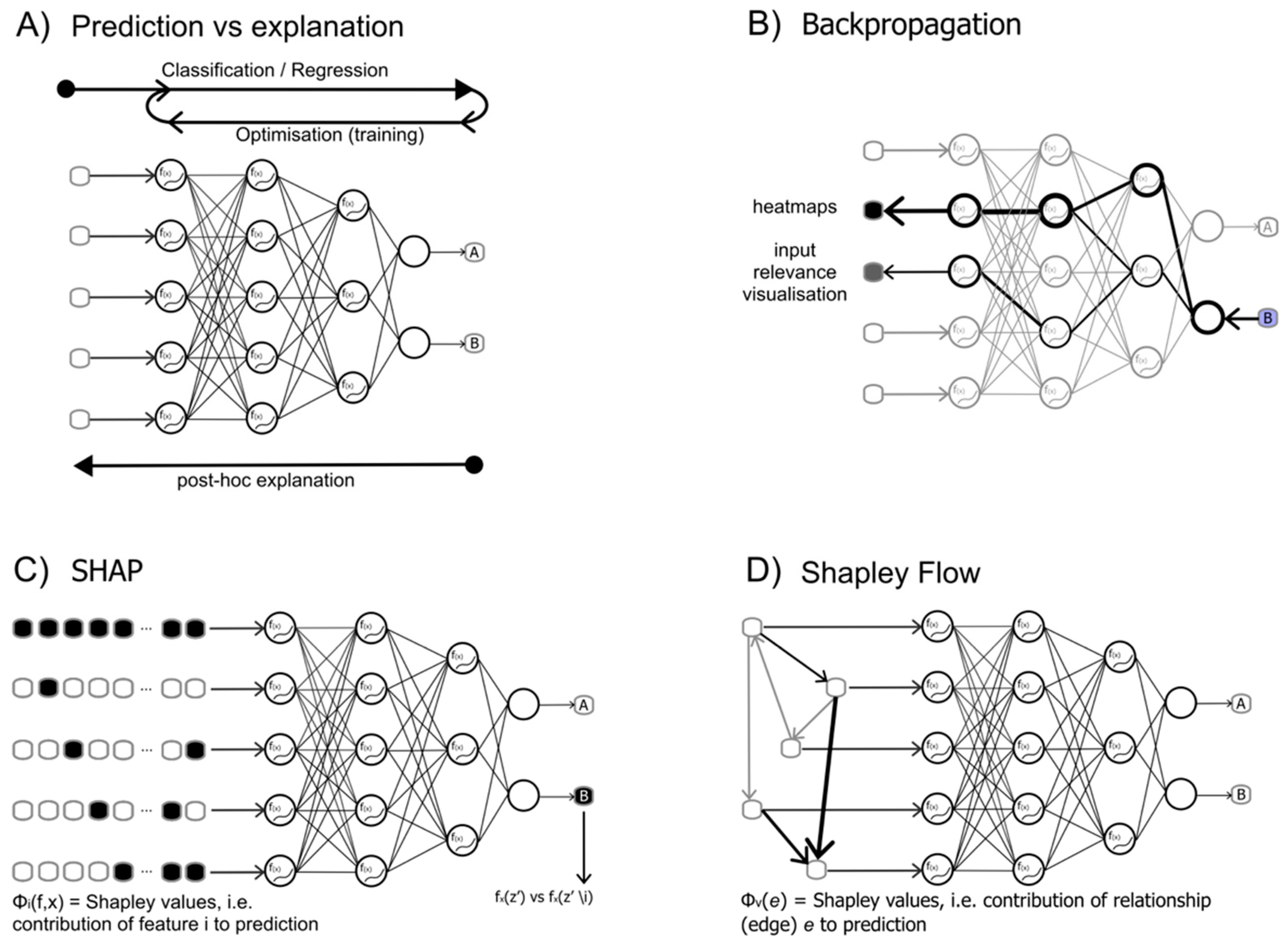
Figure 2.
The figure illustrates selected encodings of DNA sequences used in the studies which used explainable deep learning for genomics applications. One of the most frequently used encoding is called “one-hot encoding”, which converts a DNA sequence into a matrix of four rows, each row representing the presence/absence of a DNA base in each position. This method has the advantage of being quite simple and straightforward, and is also suitable for deconvolution architectures, when different kernels are applied to the resulting image, as represented in the figure. Other approaches include counting the occurrence of different features (motifs, sequence combinations) in sliding windows across the input sequence, (k-mer counting or bin feature counts). Genotype-based encodings most frequently use a minor allele count or raw encoding of the three possible genotypes, or alternatively represent each genotype with a combination of 0 and 1 depending on the present/absence of each major/minor allele. The figure also shows which explainability methods have been used with the illustrated encodings.
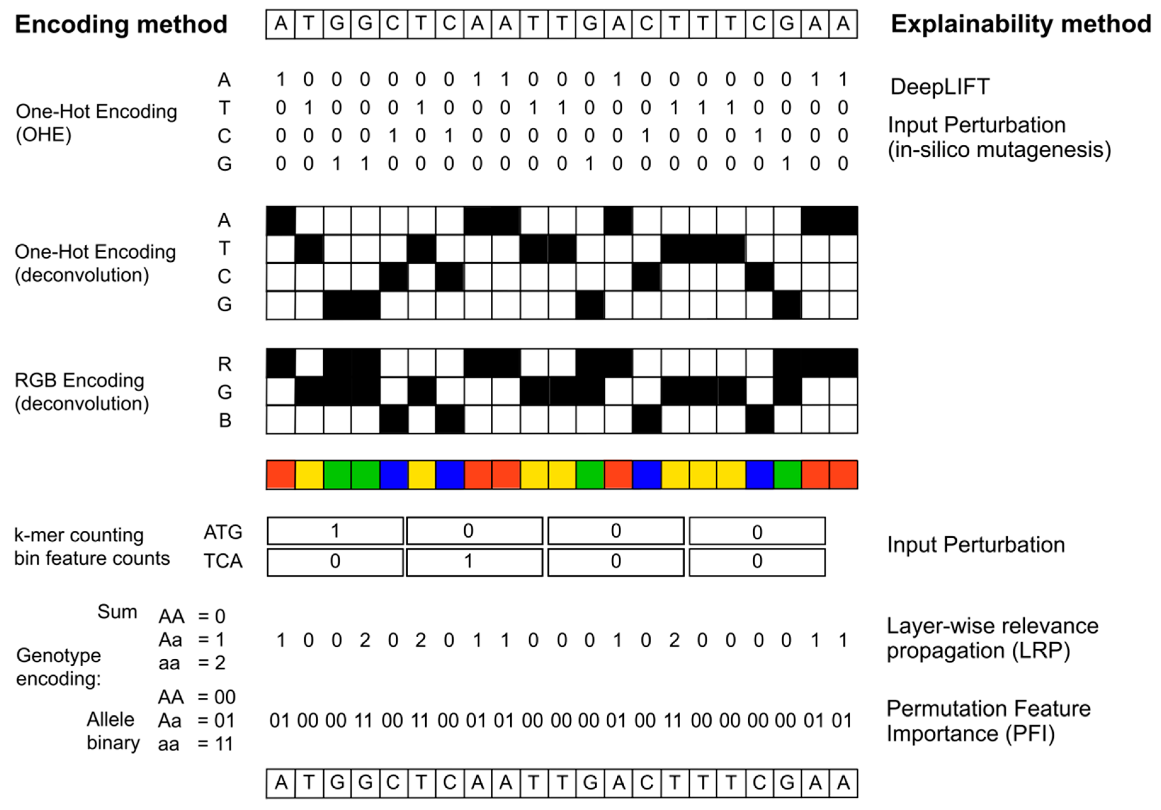

Table 1.
Selected explainability methods, belonging to the categories represented in Figure 1, have been listed, along with their code repository and suggested tutorials one could use to approach the method and learn how to implement it.
Table 1.
Selected explainability methods, belonging to the categories represented in Figure 1, have been listed, along with their code repository and suggested tutorials one could use to approach the method and learn how to implement it.
| Method | Description | Code | Tutorial | Reference |
|---|---|---|---|---|
| LRP | The acronym stands for Layer-wise Relevance Propagation, and is a method that explains graphs (originally) and deep neural networks by propagating the outcome decision backward across the neural network. | https://github.com/sebastian-lapuschkin/lrp_toolbox | https://colab.research.google.com/drive/166FYIwxblfrEltkYqY_jiJoAm9VLMweJ?usp=sharing | Bach et al. 2015, Lapuschkin et al. 2016 |
| https://git.tu-berlin.de/gmontavon/lrp-tutorial | ||||
| DeepLift | The acronym stands for "Deep Learning Important FeaTures" and works in a similar way to LRP furher implementing additional rules on how to distribute the relevance during backpropagation. | https://github.com/kundajelab/deeplift | https://www.youtube.com/playlist?list=PLJLjQOkqSRTP3cLB2cOOi_bQFw6KPGKML | Shrikumar A. et al |
| GradCAM | The name stands for Gradient-weighted Class Activation Mapping, and it is a method that exploits the gradients of any output to produce a localisation map highlighting the most important regions in an input image for predicting the output. | https://keras.io/examples/vision/grad_cam/ | https://colab.research.google.com/drive/1bA2Fg8TFbI5YyZyX3zyrPcT3TuxCLHEC?usp=sharing | Selvaraju et al. 2017 |
| https://github.com/ismailuddin/gradcam-tensorflow-2/blob/master/notebooks/GradCam.ipynb | ||||
| SHAP | SHAP stands for "SHapley Additive exPlanations", a method derived from game theory and aimed at measuring the contribution of each input feature into a prediction. The method helps with both local and global interpretability. | https://github.com/slundberg/shap | https://www.kaggle.com/code/dansbecker/shap-values | Lundberg and Lee, 2017 |
| https://towardsdatascience.com/a-complete-shap-tutorial-how-to-explain-any-black-box-ml-model-in-python-7538d11fae94 | ||||
| Shapely Flow | A further development on the SHAP algorithm, where relationships (dependency structure) between input variables are described with a graph: Shapley values are then attributed asimmetrically using this information, but are assigned to the relationships rather than the variables. | https://github.com/nathanwang000/Shapley-Flow | https://github.com/nathanwang000/Shapley-Flow/blob/master/notebooks/tutorial.ipynb | Wang et al. 2021 |
Disclaimer/Publisher’s Note: The statements, opinions and data contained in all publications are solely those of the individual author(s) and contributor(s) and not of MDPI and/or the editor(s). MDPI and/or the editor(s) disclaim responsibility for any injury to people or property resulting from any ideas, methods, instructions or products referred to in the content. |
© 2023 by the authors. Licensee MDPI, Basel, Switzerland. This article is an open access article distributed under the terms and conditions of the Creative Commons Attribution (CC BY) license (http://creativecommons.org/licenses/by/4.0/).
Copyright: This open access article is published under a Creative Commons CC BY 4.0 license, which permit the free download, distribution, and reuse, provided that the author and preprint are cited in any reuse.


