
Submitted:
20 February 2023
Posted:
22 February 2023
You are already at the latest version
Abstract
Building fires are preventable incidents that have proven to be both deadly and costly. Addressing their root causes will lead to safer neighbourhoods for families and businesses to live and operate in. Multiple studies have established the effect of residents’ socioeconomic compositions on an area’s building fire rates; however, the existing model based on the classical stepwise regression procedure has several limitations. This paper aims to construct a more accurate predictive model of building fire rates based on a set of explanatory socioeconomic variables. In building the socioeconomic model, a backward elimination by Robust Final Predictor Error (RFPE) criterion is proposed to enhance the forecasting capability of the model. The proposed method has been implemented on the census data and the fire incident data of the South East Queensland region in Australia. A cross-validation was then conducted to assess the model’s accuracy. In addition, comparative analyses of other elimination criteria, such as p-value, adjusted R-squared, Akaike’s Information Criterion (AIC), Bayesian Information Criterion (BIC) and predicted residual error sum of squared (PRESS), were conducted. The cross-validation analyses demonstrate that the proposed criterion is a more accurate predictive model based on a couple of goodness-of-fit measures. All in all, the RFPE equation was found to be a suitable criterion for the backward elimination procedure in the socioeconomic modelling of building fires.
Keywords:
Building fire
; Socioeconomic determinants
; South East Queensland
; Predictive model
; Forecasting
; Backward elimination
; Robust final predictor error
1. Introduction
Building fire is a continuing concern for households, businesses and authorities throughout Australia. In a single year, the country spent over $2.5 billion on fire protection products and services [1]. Despite the enormous expenditure, building fires still took the life of 51 Australians in 2020 [2]. Additionally, it cost Australia’s economy 1.3 per cent of the country’s Gross Domestic Product (GDP) [3]. The amount was an accumulation of losses due to injury, property damages, environmental damages, destruction of heritage and various costs to impacted businesses. The state of Queensland itself recorded 1,554 fire incidents involving damages to building structures and contents in 2020 alone [4]. Every single incident is about a Queenslander who has lost a family home, a loved one or a livelihood that has fed generations of Australians. Therefore, continued effort to understand and limit the incidence of fires is warranted.
Studies linking socioeconomic data to building fires have been conducted in various jurisdictions using different quantitative and qualitative methodologies. Lizhong, et al. [5] established the relationship between GDP-per-capita and education level to fire rate and fire death rate in Jiangsu, Guangdong and Beijing, China. It adopted the partial correlation analysis to compute the correlation coefficient of every variable pairing. In Cook County, United States, geocoding and visual mapping connected poverty rates to higher 'confined fires' incident rates in one-family and two-family dwellings [6]. Logistic regression is also used to identify relevant socioeconomic variables through four implementations within a four-stage conceptual framework [7]. The study utilises the census data of New South Wales residents and the corresponding variables selected to calculate indexes within the Socioeconomic Indexes for Areas (SEIFA) project.
Other methodologies have also adopted algorithms to not only assign coefficients but also select variables that build the most fitting model. For example, Chhetri, et al. [8] utilised the classical stepwise regression method and discriminant factor analysis (DFA) to select predictive determinants from variables identified in the technical papers of the Socioeconomic Indexes for Areas (SEIFA). As a result, it managed to capture variables that possess high t-statistics. However, its use of the classical stepwise regression method, as proposed by Efroymson [9], has been known for several limitations. Critics have also discouraged its use of t-statistics or p-value elimination criteria and the forward selection procedure to build statistical models [10,11,12,13,14]. The limitations of the classical stepwise regression method can be summarised into five issues – overreliance on chance, overstated significance, lack of guarantee for global optimisation, inconsistency-causing collinearity and non-contingency of outliers [10,11,12,13,14]. In addition, the method has been shown to provide poorer accuracy than the Principal Component Analysis (PCA) [15]. Therefore, the methodology was improved in a study in West Midlands, U.K., by adding PCA to discover the most predictive variables or components [16].
Similar to the West Midlands study, this paper also attempts to improve the methodology in Chhetri, Corcoran, Stimson and Inbakaran [8]. We propose a backward elimination by the Robust Final Prediction Error (RFPE) criterion to model the socioeconomic determinants of building fires. Such modifications to the model-building algorithm and elimination/selection criterion have the potential to produce a socioeconomic model that makes superior predictive accuracies. Additionally, the resulting model may make more cautious representations of individual parameters’ influence, preventing false confidence and reflecting the real world more accurately. The contribution of this paper includes the first application of the backward elimination by RFPE criterion and the comparative analysis of RFPE to other criteria applicable to the backward elimination procedure. Over and above that, the paper aims to play a part in improving the effectiveness of future fire safety regulations and programs that better protect households with the identified socioeconomic risk profile.
In assessing the method’s suitability, this paper delivers in six sections—the subsequent Section 2 reviews related work to explore the limitations of the classical regression method. Next, Section 3 describes the proposed robust backward elimination method by the RFPE criterion. A case study applied for South East Queensland is presented in Section 4. Afterwards, Section 5 details the available alternative criteria to the backward elimination procedure and the comparative analysis of the proposed criterion. Finally, Section 6 concludes the paper by discussing the study’s findings and future research directions.
2. Related Work
Before going into the method’s ingrained limitations, the common purpose of adopting the classical regression method has to be understood. Often, researchers adopted the method to disregard ‘insignificant’ variables to achieve parsimony, i.e., ‘simpler’ equations [10,11]. Then, the parsimonious model is inferred for the explanatory variables’ individual influences on the dependent variable [13,14]. Others utilise the resulting model for prediction and forecasting purposes [10,17].
Chhetri, Corcoran, Stimson and Inbakaran [8] conducted an ingenious study to model socioeconomic determinants of building fires. It has resourcefully identified the Index of Socioeconomic Advantages and Disadvantages (IRSAD) by the Australian Bureau of Statistics (ABS) as a suitable pool for candidate explanatory variables. In addition, the study uses discriminant function analysis (DFA) to identify determinants of fires in different suburbs – the culturally diversified and economically disadvantaged suburbs, the predominantly traditional family suburbs and the high-density inner suburbs with community housing. However, one subsection uses classical stepwise regression to identify the overall socioeconomic determinants of building fires. Although there are many valid uses of the method as an exploratory tool, misguided confidence and interpretations are likely to mislead research conclusions.
The limitations of the classical stepwise regression can be summarised into five issues – overreliance on chance, overstated significance, lack of guarantee for global optimisation, inconsistency-causing collinearity and non-contingency of outliers which can be described one by one, as follows.
2.1. Limitation 1: Over-Reliance on Chance
There is a high probability of the regression failing to identify actual causal variables. One of the main reasons is that the set of variables might, by chance, affect the particular training datasets. Without a validation process, the same variables might not show the same degree of influence if based on other sample datasets, such as datasets from other periods. The chance of nuisance variables getting selected, synonymously known as type I error, has been quantified by multiple studies such as the one by Smith [11]. Apart from referencing experiments that show poor performance in small datasets [18,19], Smith [11] conducts a series of Monte Carlo simulations to show that stepwise regression can include nuisance variables 33.5% of the time while choosing from 50 candidate variables. The rate almost tripled when the method was utilised for 1000 candidate variables. The simulations also found that at least one valid variable is not selected 50.5% of the time in choosing from 100 candidate variables [11]. The main reason for the limitation is that the statistical tests used in stepwise regression are designed for priori, i.e. the tests are made to quantify a model that has been previously built or established, for example, through expert knowledge and causation studies [10]. It is never intended for model-building purposes. In turn, the method produced results that often presented with overstated significance.
2.2. Limitation 2: Overstated Significance
McIntyre, Montgomery, Srinivasan and Weitz [13] determine that statistical significance tests have been too liberal for any stepwise regression model since it has been ‘best-fitted’ to the dataset, biasing the data towards significance. Additionally, Smith [11] stressed that stepwise regression tends to underestimate the standard error of coefficient estimate, leading to a narrow confidence interval, overstated t-statistic and understated p-values. The phenomenon also signifies the overfitting of the model to the training dataset. In practical terms, the stepwise algorithm does not pick the set of variables that determine the response variable in the population, but it picks the set of variables that ‘best’ fit the training sample dataset.
2.3. Limitation 3: Collinearity Causes Inconsistency
Stepwise regression assumes that explanatory variables are independent of each other. Therefore, there is no provision for collinearity in the stepwise regression procedure. As a result, collinearity in stepwise regression produces high variances and inaccurate coefficient estimates [20]. These effects are again attributed to the objective of finding a model that ‘best-fit’ the training data. Models that contain different variables may have a similar fit in the presence of collinearity; therefore, the procedure will result in inconsistent results, i.e. the procedure becomes arbitrary [10,21]. Collinearity’s effect on the order of inclusion or elimination is one of the reasons for the varying outcome [22,23]. With that said, these effects are more pertinent if the purpose of adopting stepwise regression is mainly inferential [24,25,26]. As a predictive model, the inconsistency is less relevant as variables compensate for each other as their coefficients are too high or too low [26]. Therefore, the resulting function may still satisfactorily predict the dependent variable but not as reliable in estimating individual influence [26].
2.4. Limitation 4: No Guarantee of Global Optimisation
Based on the limitations discussed, it is fair to question the optimality of stepwise regression’s outcome. Thompson [27], Freckleton [21], and Smith [11] discussed whether global optimisation is achieved in stepwise regression, especially the forward selection algorithm. Since the algorithm selects variables one by one, the choice of the n-th variable depends on the (n-1)th variable. Therefore, it is reasonable to conclude that the method cannot even guarantee that the n-variable model achieved is the best-fitting n-variable equation. In other words, the local optimisation reached by conducting the stepwise regression does not guarantee that it is the global optima. In addition, the issue may also be exacerbated by erratic variable selection in multicollinear datasets. Even a small degree of multicollinearity has been shown to bias stepwise regression towards achieving local optimisation, away from global optimisation [28].
2.5. Limitation 5: Caused by Outliers
Outliers are a persistent issue in statistical analysis. They introduced bias to the most basic statistical measure, e.g. the mean value of sample data, affecting the accuracy of more advanced statistical techniques [29]. One single outlier can bias classical statistical techniques that should be optimal under normality or linearity assumptions. Firstly, population data inherently contains outliers; as the sample data gets more prominent, there is a greater likelihood of encountering outlying data points [30]. Secondly, large behavioural and social datasets are more susceptible to outliers [30,31]. Thirdly, it has been established that outliers in survey statistics of such scale are almost unpreventable, partly due to significant errors in survey responses or data entry [29,32]. Additionally, unlike the effect of collinearity, there is evidence that outliers affect inferential accuracy and a model's predictive accuracy [33].
After acknowledging the limitation of the classical stepwise regression, a natural progression should lead to exploring an alternative to the method. Although the criterion modification will not wholly replace causation studies or eliminate the same weaknesses, it will produce significantly more reliable and cautious inferences and predictions.
3. Proposed Robust Backward Elimination Method
A multivariate regression equation was sought to represent the rates of building fires based on an area’s socioceconomic composition. The resulting equation is expected to take the form of Equation (1).
where variable represents the rate of emergency services at demand area i, and represents d socioeconomic variables indexed as 0, 1, …, d respectively for demand area i. is the regression coefficient allocated to each of the d socioeconomic variables.
A backward elimination by Robust Final Predictor Error (RFPE) criterion to detect and eliminate insignificant socioeconomic variables. The use of RFPE criterion, developed by Maronna, Martin, Yohai and Salibin-Barrera [31] has the benefit of minimising the effect of outliers. The robust technique is an improvement to Akaike’s FPE criterion that can be significantly biased by outliers in the dataset [34]. The procedure is then adapted to the data sourcing and processing methodology in Chhetri, Corcoran, Stimson and Inbakaran [8] study on building fires in South East Queensland. The approach has been proposed and discussed by Untadi, et al. [35]. The proposed RFPE equation is presented in Equation (2).
where is the dataset consisting of the relevant explanatory variables xij and response variable yi. represents the supplementary data point to measure the sensitivity of the dataset to outliers. An iteratively reweighted least square algorithm derived an estimator for the error scale that is notated as σ, while stands for the robust M-estimator of an unknown parameter β [36]. The estimator for the RFPE equation is developed as in Equation (2) [31].
Equation (9) is then embedded in the backward elimination procedure as in Figure 1.
Firstly, RFPE for a model that consists of all d explanatory variables and is set as Md , is calculated. Then, every variable is eliminated and returned one by one to determine which elimination improves the RFPE of model Mk-1 the most. The algorithm removes the single variable that improves the RFPE the most. The elimination iterates until the algorithm reaches an RFPE of Mk-1 that is higher or equal to the RFPE of Mk. The termination means the algorithm assumes the subsequent iteration will not improve the model fit.
4. Case Study: South East Queensland, Australia
South East Queensland refers to a region that accounts for two-thirds of Queensland’s economy and where seventy per cent of the state’s population resides [37]. The paper defines SEQ to include the Australian Bureau of Statistics (ABS)’s twelve Statistical Area 4 (SA4) regions – Eastern Brisbane, Northern Brisbane, Southern Brisbane, WesternBrisbane, Brisbane Inner City, Gold Coast, Ipswich, Logan to Beaudesert, Northern Moreton Bay, Southern Moreton Bay, Sunshine Coast and Toowoomba. The study’s datasets are analysed at the Statistical Area 2 (SA2) level as the unit of analysis. In the 2016 Census, there were 332 SA2 areas in 12 SA4 regions in South East Queensland.
4.1. Datasets
Inspired by the methodology developed by Chhetri, Corcoran, Stimson and Inbakaran [8], the study revolves around the Australian Bureau of Statistics (ABS) technical paper for Socioeconomic Indexes for Areas (SEIFA). One of the indexes within SEIFA is the Index of Relative Socioeconomic Advantage and Disadvantage (IRSAD). In this study, the variables used to calculate IRSAD as the initial variables in the backward elimination algorithm. South East Queensland’s IRSAD is visualised in Figure 2.
The data are extracted from a 2016 Census database - '2016 Census - Counting Persons, Place of Enumeration’. It consists of tables containing aggregated values at the selected Statistical Areas, for example, the HIED dataset in Table 1. The data was accessed through the TableBuilder platform. Each category was labelled with numerical values or symbols such as &&, @@ and V.V., referring to ‘Not Stated’, ‘Not Applicable’ and ‘Overseas Visitor’, respectively. The raw data was then used to calculate the data of the corresponding variables. Every variable was a proportion of the population calculated using criteria defined for its numerator and denominator, summarised in Table 2.
On the other hand, the rate of building fires in South East Queensland was set as the response variable of the study. It was calculated based on the Queensland Fire and Emergency Services (QFES) incident data points, labelled as incident types 111, 112, 113 and 119, from 2015 to 2017 [39]. The total number of incidents throughout the three years is then cumulated, multiplied by 1,000 and divided by the number of persons counted at each SA2 area in Census 2016, resulting in the triannual rate of building fires for every 1,000 people. The data is accessible through the Queensland Government Open Data Portal.
However, inconsistency exists between QFES and ABS geographical units of data labelling. This led to QFES tagging incident locations by their state suburb (SSC), while ABS collected the relevant socioeconomic data based on its definition of SA2. The main issue brought about by the difference is that a few suburbs are located in 2-4 SA2 areas. Specifically, there are 221 suburbs out of 3,263 located in more than one SA2 area. Therefore, the study has adopted a ‘Winner Takes All’ approach by assuming overlapping suburbs as part of the SA2, where most of the suburb residents were located (50 per cent plus one). A matrix of suburb and SA2, represented as rows and columns respectively, was generated through the ABS TableBuilder platform and named ‘SSCSA2’. The ‘Winner Takes All’ approach is conducted through the code in Figure 3. It identifies the maximum value at every row and assigns the rows with a SA2 – the name of the column at which the maximum value is located.
It also has to be noted that the QFES incident data points are labelled with suburb names that contain some misspellings. For example, some identified errors include ‘Cressbrookst’ and ‘Creastmead’. Additionally, the dataset does not distinguish names used for multiple different suburbs. Therefore, the study has identified these suburb names and added parentheses, distinguishing the suburbs by following the ABS State Suburbs (SSC) naming convention and cross-referencing the postcodes of the suburbs at issue. One example is Clontarf (Moreton Bay – Qld) and Clontarf (Toowoomba – Qld).
4.2. Parameters
The results were obtained using the R software at its 2021.09.0 version on a device equipped with AMD Ryzen 5 3450U, Radeon Vega Mobile Gfx 2.10 GHz and 5.89 GB of usable RAM. In addition, the RobStatTM package was used to execute the robust stepwise regression analysis [40]. The tuning constant for the M-scale used to compute the initial S-estimator was set to 0.5. The constant determines the breakdown point of the resulting MM-estimator. Relative convergence tolerance for the iterated weighted least square (IRWLS) iterations for the MM-estimator was set to 0.001. The tolerance level was chosen to allow convergence to occur. The desired asymptotic efficiency of the final regression M-estimator was set to 0.95. Finally, the asymptotic bias optimal family of the loss function was used in tuning the parameter for the rho function.
4.3. Results
Eleven variables have been eliminated, leaving thirteen variables in the final model. Table 3 shows the variables eliminated at every step, complete with the RFPE calculation to demonstrate improvements in subsequent models. A detailed model specification, which includes a coefficient ad for every retained variable gd, (see Eqn. 1) was contained in Table 4.
Overall, the model’s R-squared was calculated to be 0.4259, translating to 42.59 per cent of variations explainable by the variables retained. The adjusted R-squared of 0.4024 has indicated the model R-squared upon fitting to another dataset in the population. The figure sufficiently satisfies the threshold set by Falk and Miller [41] for endogenous constructs such as the one obtained. A robust residual standard error (RSE) of 0.3779 meant the observed building fire rates were off from the actual regression line by approximately 0.3779 units on average.
In identifying the individual parameters' influence, an abundance of caution has to be exercised as a model-building algorithm is known to overstate significance [11]. Further assessment, for example, through Monte Carlo simulations, is recommended. Four socioeconomic variables, CHILDJOBLESS, NOCAR, OCC_MANAGERS and UNEMPLOYED, were significant at the 0.001 level. Based on their t-statistics and F-statistics, the corresponding p-values (0.000106, 6.77e-07, 5.68e-07 and 0.000141 respectively) preliminarily indicated the variables’ inclusions are not due to chance. UNEMPLOYED highest positive coefficient increases building fire rates to the highest degree, while OCC_SERVICE_L lowest negative coefficient decreases building fire rates the most significantly.
The model's forecasting ability is further scrutinised through the following plots in Figure 4 and Figure 5.
The plot of response value against its fitted values in Figure 4 compares the model’s supposed rates of building fires and the actual rates. Most suburbs are evidently scattered around the identity line where the ratio of the two sets of values is one-to-one, showing a visually representative equation of the data points’ behaviour. Additionally, it shows data points labelled 105, 259 and 276 – representing Eagle Farm to Pinkenba, Rocklea to Acacia Ridge and Southern Southport as outliers. This is because the rates of building fires in these regions are exceptionally higher.
In Figure 4, the three outlying points are again highlighted because they are significant leverage points. It means that the outliers may have a significant influence on biasing the goodness-of-fit of the model. Most other data points can be classed as regular – not leverage points nor outliers. Additionally, there are also nine points with high leverage, i.e. they have the potential to influence the model dramatically.
Cross-validation is then conducted to investigate if the criteria and procedure have produced a model that is applicable to the dataset that is not used to train the model. The Root of the Mean of the Square of Errors (RMSE) in Equation (14) and the Mean of Absolute value of Errors (MAE) in Equation (15) are used as the basis for comparison.
where yi is the actual rate of building fires, yp is the projected rate of building fires and n is the number of observations/suburbs.
The cross-validation procedure is showcased in Figure 6, along with the resulting goodness-of-fit measures in Table 5.
Table 5 shows negligible differences between the root-mean-square error (RMSE) and mean absolute error (MAE). An exception was observed in the iteration with the third fold as the testing dataset. A substantial difference was detected; however, the average difference across the five iterations is still negligibly low. This indicates the model’s equal performance on a dataset not involved in training the model obtained through the proposed method.
5. Comparative Study
5.1. Alternative Backward Elimination Criteria
There are sizeable alternative criteria to equip the backward elimination in assessing the goodness-of-fit of a model. Therefore, this paper adopts four criteria as the comparative basis for the RFPE criterion.
5.1.1. Adjusted R-Squared
R-squared is biased against a model with more parameters or explanatory variables, therefore, influencing the algorithm to favour parsimonious models. Ezekiel [42] sought to counteract this effect by adjusting the R-squared equation. Adjusted R-squared can be interpreted as a less biased estimator of the population R-squared, whereas the observed sample R-squared is a positively biased estimate of the population value [43]. The difference to the classical R-squared includes a penalty for the inclusion of redundant variables by multiplying the equation, (n — 1)/(n — p) [44]. The adjusted R-squared is defined and simplified as follows.
where p is the total number of explanatory variables in the model, and n is the sample size.
5.1.2. Akaike Information Criterion (AIC)
Akaike [45] proposed an indicator for a model’s quality by measuring its goodness-of-fit by estimating Kullback-Leibler divergence using the maximum likelihood principle. The Akaike’s Information Criterion (AIC) is proposed as follows [46].
where k is the number of parameters, L represents the maximum likelihood function of the parameter estimate , given the data y. The criterion can be embedded within a backward elimination algorithm as follows [47].
where k is the number of parameters, n is the sample size, and RSS is the residual sum of squares of the model. Stepwise AIC algorithm has been implemented in financial, medical and epidemiological applications [48,49,50].
The AIC is the most commonly used information theoretic approach to measuring how much information is lost between a selected model and the true model. It has been used widely as an effective model selection method in many scientific fields, including ecology and phylogenetics [51,52]. Compared with the use of adjusted R-squared to evaluate the model solely on fit, AIC also considers model complexity [51].
5.1.3. Bayesian Information Criterion (BIC)
Bayesian Information Criterion, also known as Schwarz Information Criterion, was proposed by Gideon Schwarz [53]. Modifying Akaike’s Information Criterion by introducing Bayes estimators to estimate the maximum likelihood of the model’s parameters. The BIC is formulated as follows.
where k is the number of parameters, L represents the maximum likelihood function of the parameter estimate , given the data y. Similarly to AIC, the BIC are applicable to the backward elimination algorithm as follows.
where k is the number of parameters, n is the sample size, and RSS is the residual sum of squares of the model.
The strength of BIC includes its ability to find the true model if it exists within the candidates. However, it comes with a significant caveat, as the existence of a true model that reflects reality is debatable. Although BIC penalises overfitting on larger models, preferring a more parsimonious or lower-dimensional model. However, for its predictive ability, AIC is better because it minimises the mean squared error of prediction/estimation [54].
5.1.4. Predicted Residual Error Sum of Squares (PRESS)
Allen [55] developed an indicator of a model’s fit through the predicted residual error sum of squares (PRESS) statistic. The differentiation to the statistic at that time is its ability to measure fit based on samples that are not used to form a model [55,56]. The statistic is a cross-validation attempt by a leave-one-out method that subtracts and leaves the i-th observation out, reducing the sample size to n – 1 [57]. Repeating the subtraction and omission to every single data point will lead to the sum of squares of discrepancies [58,59]. PRESS is formulated as follows.
5.2. Comparison to Akaike’s Information Criterion (AIC) Criterion
Twelve variables have been eliminated, leaving sixteen variables in the final model. Table 6 shows the variables eliminated at every step, complete with the RFPE calculation to demonstrate improvements in subsequent models. A detailed model specification, which includes a coefficient ad for every retained variable gd, (see Eqn. 1) was contained in Table 7.
Overall, the model’s R-squared was calculated to be 0.4730, translating to 47.30 per cent of variations explainable by the variables retained. The adjusted R-squared of 0.4532 has indicated the model R-squared upon fitting to another dataset in the population. The figure sufficiently satisfies the threshold set by Falk and Miller [41] for endogenous constructs such as the one obtained. A robust residual standard error (RSE) of 0.4544 meant the observed rate of the building fires was off from the actual regression line by approximately 0.4544 units on average. The following section provides a comparative benchmark to assess the quality of the RSE.
The same cautions should be applicable for a reason provided in Section 4.1. CERTIFICATE, CHILDJOBLESS, HIGHBED, INC_HIGH, NOCAR and OCC_MANAGERS were identified as having the most significant relationships to the response variable based on their t-statistics and F-statistics. They were shown to have p-values (7.45e-06, 0.000384, 2.31e-06, 0.000106 and 2.26e-09 respectively) significant at the 0.001 level. Therefore, these variables fluctuate building fire rates to the highest degree.
The model’s forecasting ability is compared to the one produced by using the RFPE criteria through the following plots in Figure 7.
Both models’ Q-Q plots are similarly right-skewed or positively skewed, as showcased in Figure 7a,b. Regardless, the data points remain generally on the linear line, crowding towards the zero quantiles. Therefore, both are normally distributed with a heavy right tail. Subsequently, the plot of the residual-fitted value shows that deviations to the model produced using the RFPE criterion are slightly more well-behaved than that of the AIC criterion. The relatively straighter line in Figure 7c is predominantly biased by one point. The rest of the points scatter randomly around the zero line; therefore, Gauss-Markov’s assumption of linearity is more convincing than that of Figure 7d. Furthermore, both models are also compared on their goodness-of-fit in Table 8.
The two models are comparable on RMSE and MAE. The model produced through the RFPE criterion resulted in a lower MAE, but a higher RMSE than the model produced through the AIC criterion. To investigate further, the same cross-validation procedure in Figure 6 is then applied to the model produced using the AIC criterion. The results are contained in Table 9.
Based on the RMSE and MAE measure, the RFPE criterion fares slightly better than the AIC. This is consistent with the robust premise of the RFPE criterion that sought to reduce the effect of outliers on the resulting model. Since RMSE punishes the model with large error against the outliers, it conforms that model produced using RFPE criterion has higher training RMSE, but a lower testing RMSE.
5.3. Comparison to Other Criteria
For comparative purposes, the study has also adopted p-value, adjusted R-squared, BIC and PRESS as criteria for the backward elimination procedure. The methods are carried out using the ‘SignifReg’ package in the R environment. The criteria are consistent with their respective equation in Section 5.1. Using the entire dataset for training, the resulting model from each criterion is assessed for their goodness-of-fit, as in Table 10.
The models are shown to be comparable on the three measures, although the RFPE criterion is again slightly superior on the basis of MAE. The cross-validation procedure in Figure 6 is then carried out on the four different models. The resulting goodness-of-fit measures are detailed in Table 11.
Comparing the averaged goodness-of-fit measures across the different models, the RFPE criterion still holds minuscule superiority over the averaged MAE measured on the test and train datasets. The lower MAE demonstrates the robust criterion provided by the RFPE as the MAE is not as sensitive to outliers as RMSE, indicating a model more accommodating to extreme cases [60]. Also, the robust nature of the RFPE criterion is again apparent in the third iteration, where we can observe a test dataset with a higher incidence of outliers. The RFPE criterion has produced a model with a noticeable advantage where the lower RMSE and MAE measures indicate a more resilient model that provides a better fit even to a significantly outlying dataset.
6. Conclusions
This paper has identified limitations in the prevailing socioeconomic modelling of building fires and proposed the backward elimination by Robust Final Predictor Error (RFPE) criterion to model the socioeconomic determinants of building fires. The proposed approach has been evaluated using datasets available in the region of South Eastern Queensland in Australia. A comparative study demonstrated that the proposed method is a more accurate predictive model regarding goodness-of-fit measures obtained through the cross-validation procedure. The model has relatively lower error measures, albeit the difference has not been dramatic.
Future research may involve comparing the backward elimination by the RFPE criterion to alternative approaches such as Least Absolute Shrinkage and Selection Operator (LASSO), Least Absolute Residuals (LAR) and Principal Component Analysis (PCA) [16,61,62]. Monte Carlo simulations can also be employed to assess further the resulting model's dependability for identifying individual parameters, including its measure of influence through the relevant coefficient. All in all, the paper has found sufficient justification to adopt the backward elimination with the RFPE criterion to model the socioeconomic determinants of building fires for predictive purposes.
Author Contributions
Conceptualisation, A.U., L.L., M.L. and R.D.; methodology, A.U., L.L., M.L. and R.D.; software, A.U.; resources, A.U.; data curation, A.U.; writing—original draft preparation, A.U.; writing—review and editing, L.L., M.L. and R.D.; visualisation, A.U.; supervision, L.L., M.L. and R.D.; project administration, A.U. and L.L. All authors have read and agreed to the published version of the manuscript.
Funding
The APC was funded by the Central Queensland University. The research is part of a degree that is funded by the CQUniversity Destination Australia Living Stipend Scholarship and the International Excellence Award. The scholarships are jointly funded by the Central Queensland University and the Destination Australia Program.
Data Availability Statement
Restrictions apply to the availability of these data. Census data was obtained from the Australian Bureau of Statistics and are available at https://www.abs.gov.au/statistics/microdata-tablebuilder/tablebuilder with the permission of the Australian Bureau of Statistics. Queensland Fire and Emergency Services (QFES) incident data was obtained from the Queensland Fire and Emergency Services and are available at https://www.data.qld.gov.au/dataset/qfes-incident-data with the permission of the Queensland Fire and Emergency Services.
Conflicts of Interest
The authors declare no conflict of interest.
References
- Kelly, A. Fire Protection Services in Australia; IBISWorld: May 2022.
- Australian Bureau of Statistics. Causes of Death, Australia. Available online: https://www.abs.gov.au/statistics/health/causes-death/causes-death-australia/2020} (accessed on 1 December 2022).
- Ashe, B.; McAneney, K.J.; Pitman, A.J. Total cost of fire in Australia. Journal of Risk Research 2009, 12, 121-136. [CrossRef]
- Queensland Fire and Emergency Services. QFES Incident Data. 2020.
- Lizhong, Y.; Heng, C.; Yong, Y.; Tingyong, F. The Effect of Socioeconomic Factors on Fire in China. Journal of Fire Sciences 2005, 23, 451-467. [CrossRef]
- Fahy, R.; Maheshwari, R. Poverty and the risk of fire; National Fire Protection Organisation: 2021.
- Tannous, W.K.; Agho, K. Socio-demographic predictors of residential fire and unwillingness to call the fire service in New South Wales. Preventive Medicine Reports 2017, 7, 50-57. [CrossRef]
- Chhetri, P.; Corcoran, J.; Stimson, R.J.; Inbakaran, R. Modelling Potential Socioeconomic Determinants of Building Fires in South East Queensland. Geographical Research 2010, 48, 75-85. [CrossRef]
- Efroymson, M.A. Multiple regression analysis. Mathematical methods for digital computers 1960, 191-203.
- Harrell, F.E. Multivariable Modeling Strategies. In Regression Modeling Strategies: With Applications to Linear Models, Logistic and Ordinal Regression, and Survival Analysis, Harrell, J.F.E., Ed.; Springer International Publishing: Cham, 2015; pp. 63-102.
- Smith, G. Step away from stepwise. Journal of Big Data 2018, 5, 32. [CrossRef]
- Olusegun, A.M.; Dikko, H.G.; Gulumbe, S.U. Identifying the Limitation of Stepwise Selection for Variable Selection in Regression Analysis. American Journal of Theoretical and Applied Statistics 2015, 4, 414-419. [CrossRef]
- McIntyre, S.H.; Montgomery, D.B.; Srinivasan, V.; Weitz, B.A. Evaluating the Statistical Significance of Models Developed by Stepwise Regression. Journal of Marketing Research 1983, 20, 1-11. [CrossRef]
- Heinze, G.; Dunkler, D. Five myths about variable selection. Transplant International 2017, 30, 6-10. [CrossRef]
- Ssegane, H.; Tollner, E.W.; Mohamoud, Y.M.; Rasmussen, T.C.; Dowd, J.F. Advances in variable selection methods I: Causal selection methods versus stepwise regression and principal component analysis on data of known and unknown functional relationships. Journal of Hydrology 2012, 438-439, 16-25. [CrossRef]
- Hastie, C.; Searle, R. Socioeconomic and demographic predictors of accidental dwelling fire rates. Fire Safety Journal 2016, 84, 50-56. [CrossRef]
- Ratner, B. Variable selection methods in regression: Ignorable problem, outing notable solution. Journal of Targeting, Measurement and Analysis for Marketing 2010, 18, 65-75. [CrossRef]
- Steyerberg, E.W.; Eijkemans, M.J.C.; Habbema, J.D.F. Stepwise Selection in Small Data Sets: A Simulation Study of Bias in Logistic Regression Analysis. Journal of Clinical Epidemiology 1999, 52, 935-942. [CrossRef]
- Derksen, S.; Keselman, H.J. Backward, forward and stepwise automated subset selection algorithms: Frequency of obtaining authentic and noise variables. British Journal of Mathematical and Statistical Psychology 1992, 45, 265-282. [CrossRef]
- Cammarota, C.; Pinto, A. Variable selection and importance in presence of high collinearity: an application to the prediction of lean body mass from multi-frequency bioelectrical impedance. Journal of Applied Statistics 2021, 48, 1644-1658. [CrossRef]
- Freckleton, R.P. Dealing with collinearity in behavioural and ecological data: model averaging and the problems of measurement error. Behavioral Ecology and Sociobiology 2011, 65, 91-101. [CrossRef]
- Wang, K.; Chen, Z. Stepwise Regression and All Possible Subsets Regression in Education. Electronic International Journal of Education, Arts, and Science 2016, 2.
- Goodenough, A.E.; Hart, A.G.; Stafford, R. Regression with empirical variable selection: description of a new method and application to ecological datasets. PLoS One 2012, 7, e34338. [CrossRef]
- Siegel, A.F. Multiple Regression: Predicting One Variable From Several Others. In Practical Business Statistics (Seventh Edition), Siegel, A.F., Ed.; Academic Press: 2016; pp. 355-418.
- Seber, G.A.F.; Wild, C.J. Least Squares. In Methods in Experimental Physics, Stanford, J.L., Vardeman, S.B., Eds.; Academic Press: 1994; Volume 28, pp. 245-281.
- Wilson, J.H. Multiple Linear Regression. In Regression Analysis: Understanding and Building Business and Economic Models Using Excel; Business Expert Press: 2012.
- Thompson, B. Stepwise Regression and Stepwise Discriminant Analysis Need Not Apply here: A Guidelines Editorial. Educational and Psychological Measurement 1995, 55, 525-534. [CrossRef]
- Yuan, M.; Lin, Y. Model selection and estimation in regression with grouped variables. Journal of the Royal Statistical Society: Series B (Statistical Methodology) 2006, 68, 49-67. [CrossRef]
- Kwak, S.K.; Kim, J.H. Statistical data preparation: management of missing values and outliers. Korean J Anesthesiol 2017, 70, 407-411. [CrossRef]
- Osborne, J.W.; Overbay, A. The power of outliers (and why researchers should ALWAYS check for them). Practical Assessment, Research, and Evaluation 2004, 9. [CrossRef]
- Maronna, R.A.; Martin, R.D.; Yohai, V.J.; Salibin-Barrera, M. Robust inference and variable selection for M-estimators. In Robust Statistics; Wiley Series in Probability and Statistics; John Wiley & Sons, Incorporated: 2019; pp. 133-138.
- Wada, K. Outliers in official statistics. Japanese Journal of Statistics and Data Science 2020, 3, 669-691. [CrossRef]
- Zhang, W.; Yang, D.; Zhang, S. A new hybrid ensemble model with voting-based outlier detection and balanced sampling for credit scoring. Expert Systems with Applications 2021, 174, 114744. [CrossRef]
- Akaike, H. Statistical predictor identification. Annals of the Institute of Statistical Mathematics 1970, 22, 203-217. [CrossRef]
- Untadi, A.; Li, L.D.; Dodd, R.; Li, M. A Novel Framework Incorporating Socioeconomic Variables into the Optimisation of South East Queensland Fire Stations Coverages. In Proceedings of the Conference on Innovative Technologies in Intelligent Systems & Industrial Applications, 16-18 November, 2022, (submitted; accepted; in press).
- Maronna, R.A.; Martin, R.D.; Yohai, V.J.; Salibin-Barrera, M. M-estimators with smooth ψ-function. In Robust Statistics; Wiley Series in Probability and Statistics; John Wiley & Sons, Incorporated: 2019; p. 104.
- Queensland Government. South East Queensland Economic Foundations Paper; March 2018.
- Australian Bureau of Statistics. Technical Paper: Socioeconomic Indexes for Areas (SEIFA). 2016.
- Australasian Fire and Emergency Service Authorities Council. Australian Incident Reporting System Reference Manual. 2013.
- Salibian-Barrera, M.; Yohai, V.; Maronna, R.; Martin, D.; Brownso, G.; Konis, K.; Croux, C.; Haesbroeck, G.; Maechler, M.; Koller, M.; et al. Package ‘RobStatTM’. Available online: https://cran.r-project.org/web/packages/RobStatTM/RobStatTM.pdf (accessed on 5 December 2022).
- Falk, R.; Miller, N. A Primer for Soft Modeling. The University of Akron Press: Akron, OH 1992.
- Ezekiel, M. Methods of correlation analysis; Wiley: Oxford, England, 1930; pp. xiv, 427-xiv, 427.
- Shieh, G. Improved Shrinkage Estimation of Squared Multiple Correlation Coefficient and Squared Cross-Validity Coefficient. Organisational Research Methods 2008, 11, 387-407. [CrossRef]
- Lindsey, C.; Sheather, S. Variable Selection in Linear Regression. The Stata Journal 2010, 10, 650-669. [CrossRef]
- Akaike, H. Information Theory and an Extension of the Maximum Likelihood Principle. In Selected Papers of Hirotugu Akaike, Parzen, E., Tanabe, K., Kitagawa, G., Eds.; Springer New York: New York, NY, 1998; pp. 199-213.
- Burnham, K.P.; Anderson, D.R. Information and Likelihood Theory: A Basis for Model Selection and Inference. In Model Selection and Multimodel Inference: A Practical Information-Theoretic Approach; Springer New York: New York, NY, 2002; pp. 49-97.
- Venables, W.N.; Ripley, B.D. Linear Statistical Models. In Modern Applied Statistics with S; Springer New York: New York, NY, 2002; pp. 139-181.
- Zhang, T.; Zhang, J.; Liu, Y.; Pan, S.; Sun, D.; Zhao, C. Design of Linear Regression Scheme in Real-Time Market Load Prediction for Power Market Participants. In Proceedings of the 2021 11th International Conference on Power and Energy Systems (ICPES), 18-20 Dec. 2021, 2021; pp. 547-551.
- Luu, M.N.; Alhady, S.T.M.; Nguyen Tran, M.D.; Truong, L.V.; Qarawi, A.; Venkatesh, U.; Tiwari, R.; Rocha, I.C.N.; Minh, L.H.N.; Ravikulan, R.; et al. Evaluation of risk factors associated with SARS-CoV-2 transmission. Current Medical Research and Opinion 2022, 1-8. [CrossRef]
- Hevesi, M.; Dandu, N.; Darwish, R.; Zavras, A.; Cole, B.; Yanke, A. Poster 212: The Cartilage Early Return for Transplant (CERT) Score: Predicting Early Patient Election to Proceed with Cartilage Transplant Following Chondroplasty of the Knee. Orthopaedic Journal of Sports Medicine 2022, 10, 2325967121S2325900773. [CrossRef]
- Johnson, J.B.; Omland, K.S. Model selection in ecology and evolution. Trends Ecol Evol 2004, 19, 101-108. [CrossRef]
- Sullivan, J.; Joyce, P. Model Selection in Phylogenetics. Annual Review of Ecology, Evolution, and Systematics 2005, 36, 445-466. [CrossRef]
- Schwarz, G. Estimating the Dimension of a Model. The Annals of Statistics 1978, 6, 461-464.
- Vrieze, S.I. Model selection and psychological theory: A discussion of the differences between the Akaike information criterion (AIC) and the Bayesian information criterion (BIC). Psychological Methods 2012, 17, 228-243. [CrossRef]
- Allen, D.M. The Relationship Between Variable Selection and Data Agumentation and a Method for Prediction. Technometrics 1974, 16, 125-127. [CrossRef]
- Tarpey, T. A Note on the Prediction Sum of Squares Statistic for Restricted Least Squares. The American Statistician 2000, 54, 116-118. [CrossRef]
- Qian, J.; Li, S. Model Adequacy Checking for Applying Harmonic Regression to Assessment Quality Control. ETS Research Report Series 2021, 2021, 1-26. [CrossRef]
- Quan, N.T. The Prediction Sum of Squares as a General Measure for Regression Diagnostics. Journal of Business & Economic Statistics 1988, 6, 501-504. [CrossRef]
- Draper, N.R.; Smith, H. Applied Regression Analysis, 2nd ed.; John Wiley: New York, 1981.
- Hodson, T.O. Root-mean-square error (RMSE) or mean absolute error (MAE): when to use them or not. Geosci. Model Dev. 2022, 15, 5481-5487. [CrossRef]
- Haem, E.; Harling, K.; Ayatollahi, S.M.T.; Zare, N.; Karlsson, M.O. Adjusted adaptive Lasso for covariate model-building in nonlinear mixed-effect pharmacokinetic models. Journal of Pharmacokinetics and Pharmacodynamics 2017, 44, 55-66. [CrossRef]
- Kim, H.R. Model Building with Forest Fire Data: Data Mining, Exploratory Analysis and Subset Selection. 2009.
Figure 1.
Algorithm of the Robust Backward Elimination by RFPE.
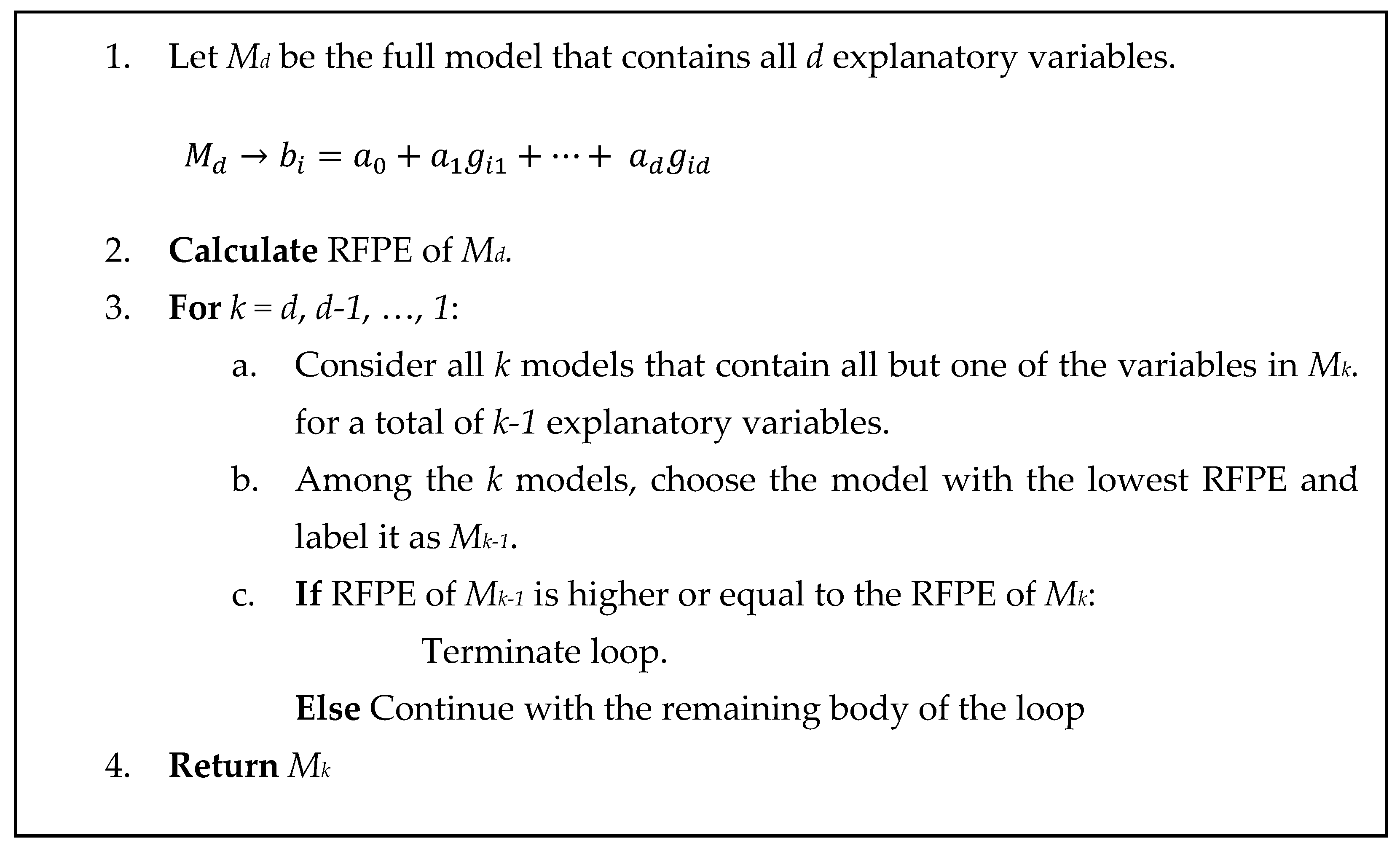
Figure 2.
Visualisation of SEIFA scores on the map of South East Queensland [38].
Figure 2.
Visualisation of SEIFA scores on the map of South East Queensland [38].
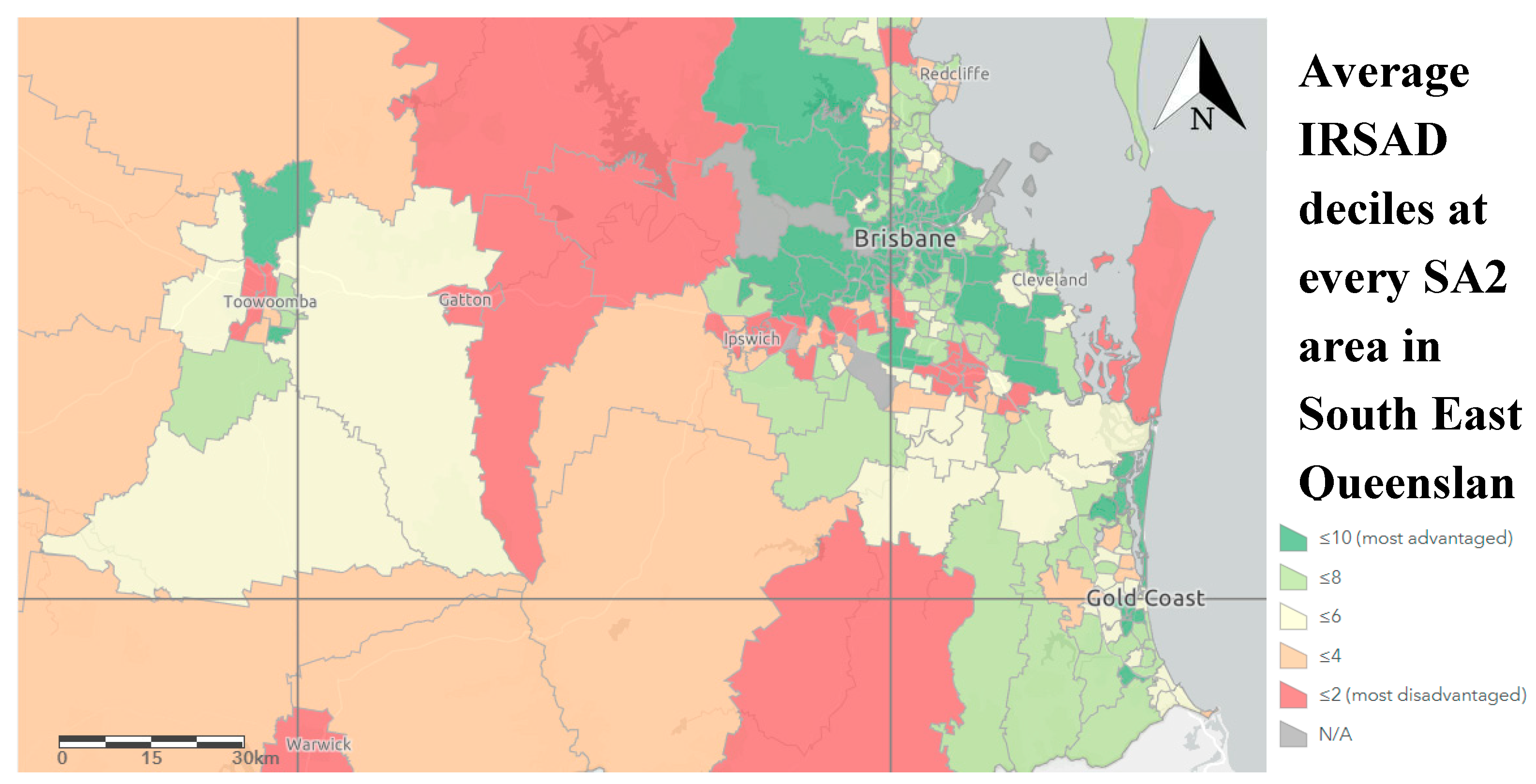
Figure 3.
Code snippet for the ‘Winner Takes All’ approach in R.

Figure 4.
Response – Fitted Values plot for the model by RFPE criterion.
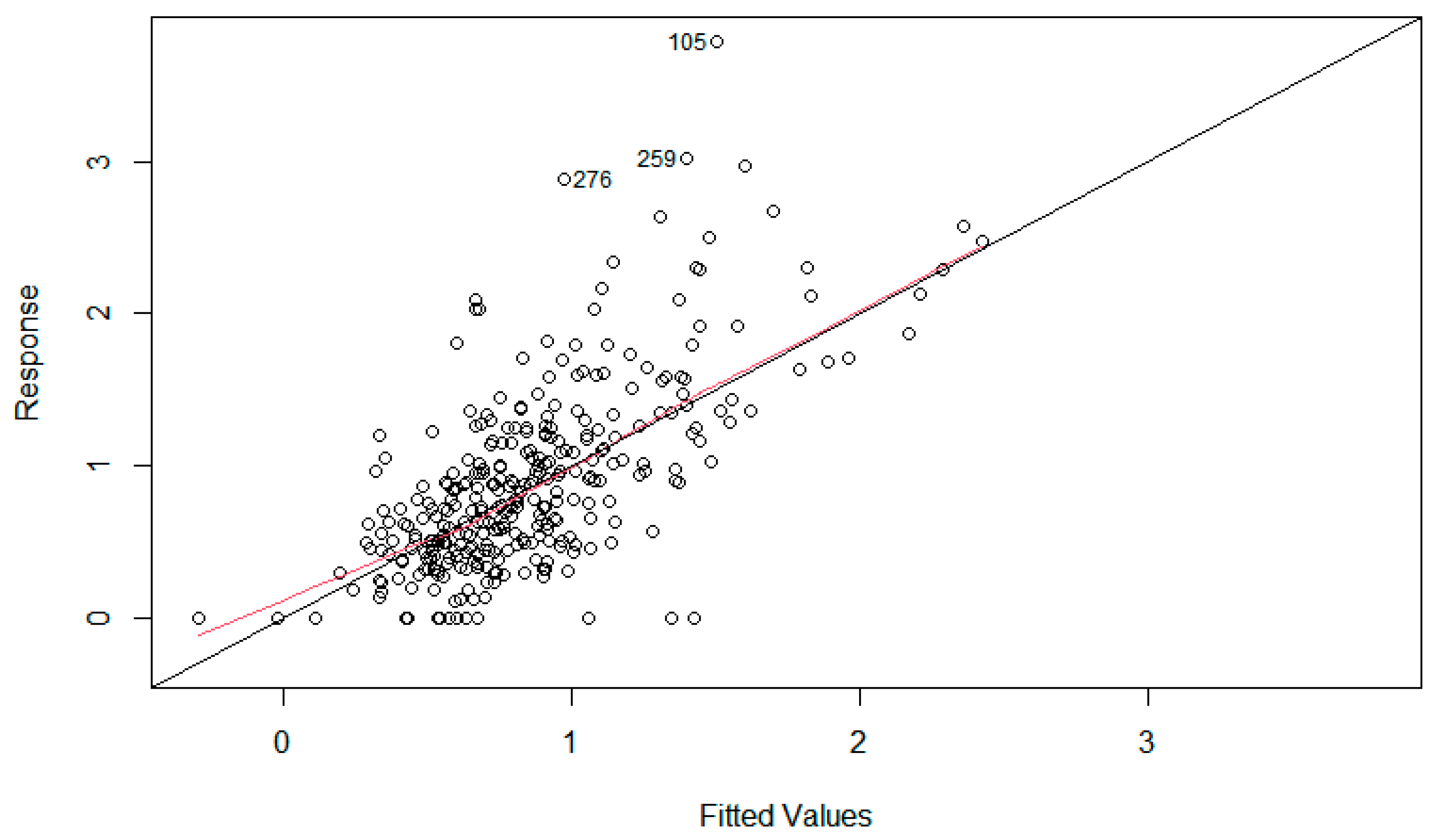
Figure 5.
Standardised Residuals – Distances plot for the model by RFPE criterion.
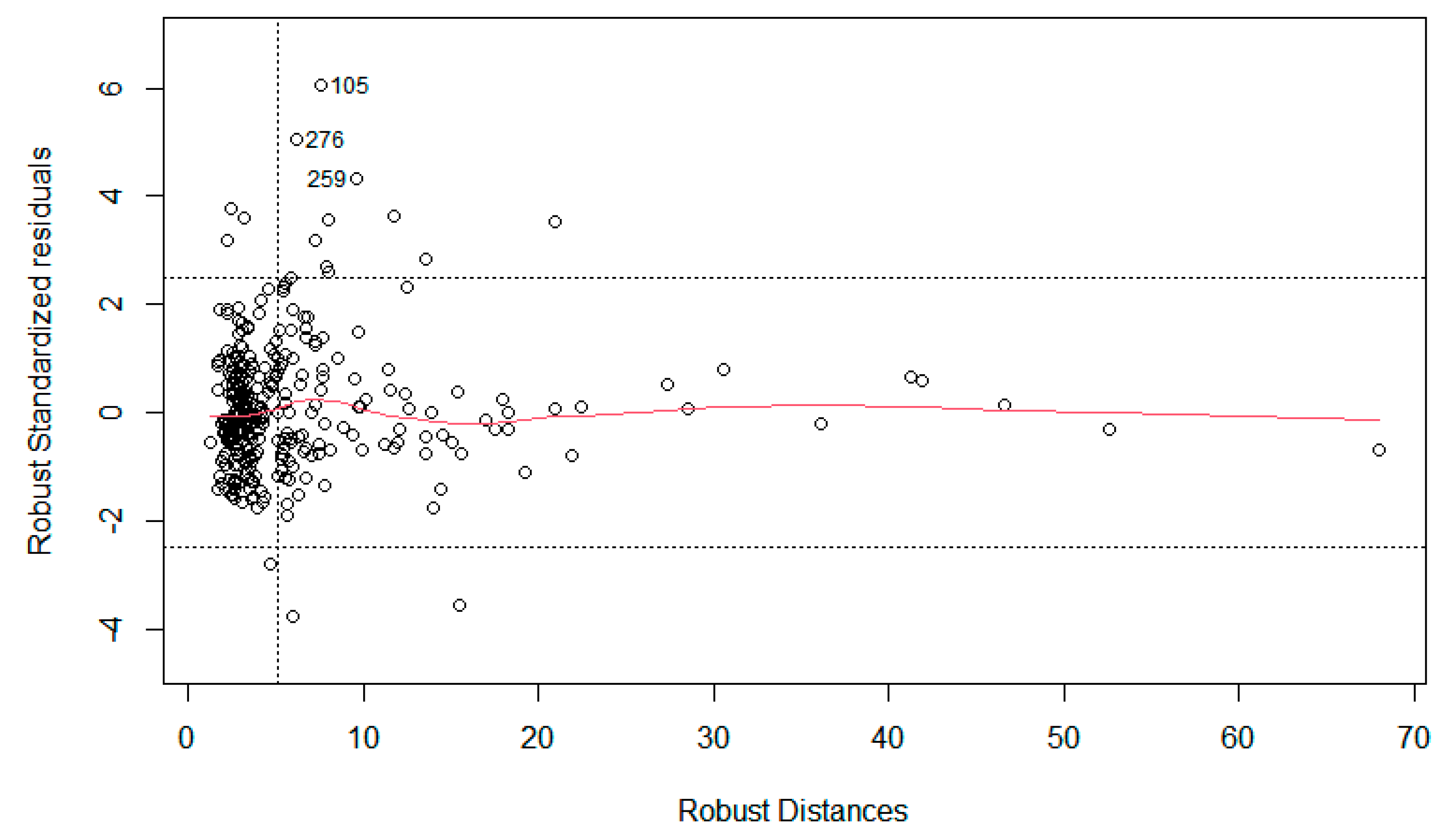
Figure 6.
Algorithm of the 5-fold cross-validation.
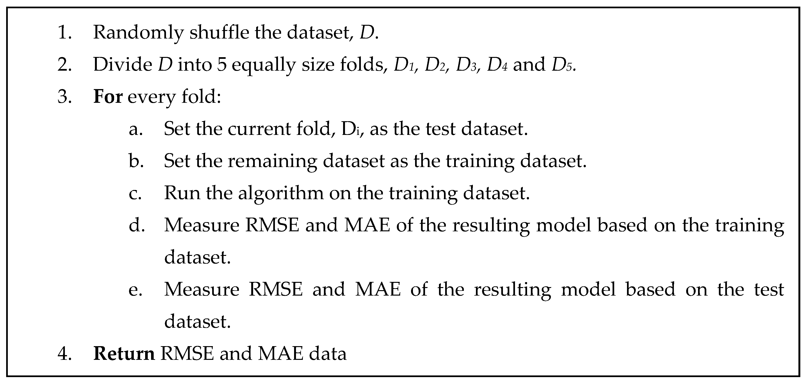
Figure 7.
Q-Q plots for models produced through backward elimination using (a) RFPE criterion and (b) AIC criterion. Residuals against fitted values plots for models produced through backward elimination using (c) RFPE criterion and (d) AIC criterion.
Figure 7.
Q-Q plots for models produced through backward elimination using (a) RFPE criterion and (b) AIC criterion. Residuals against fitted values plots for models produced through backward elimination using (c) RFPE criterion and (d) AIC criterion.
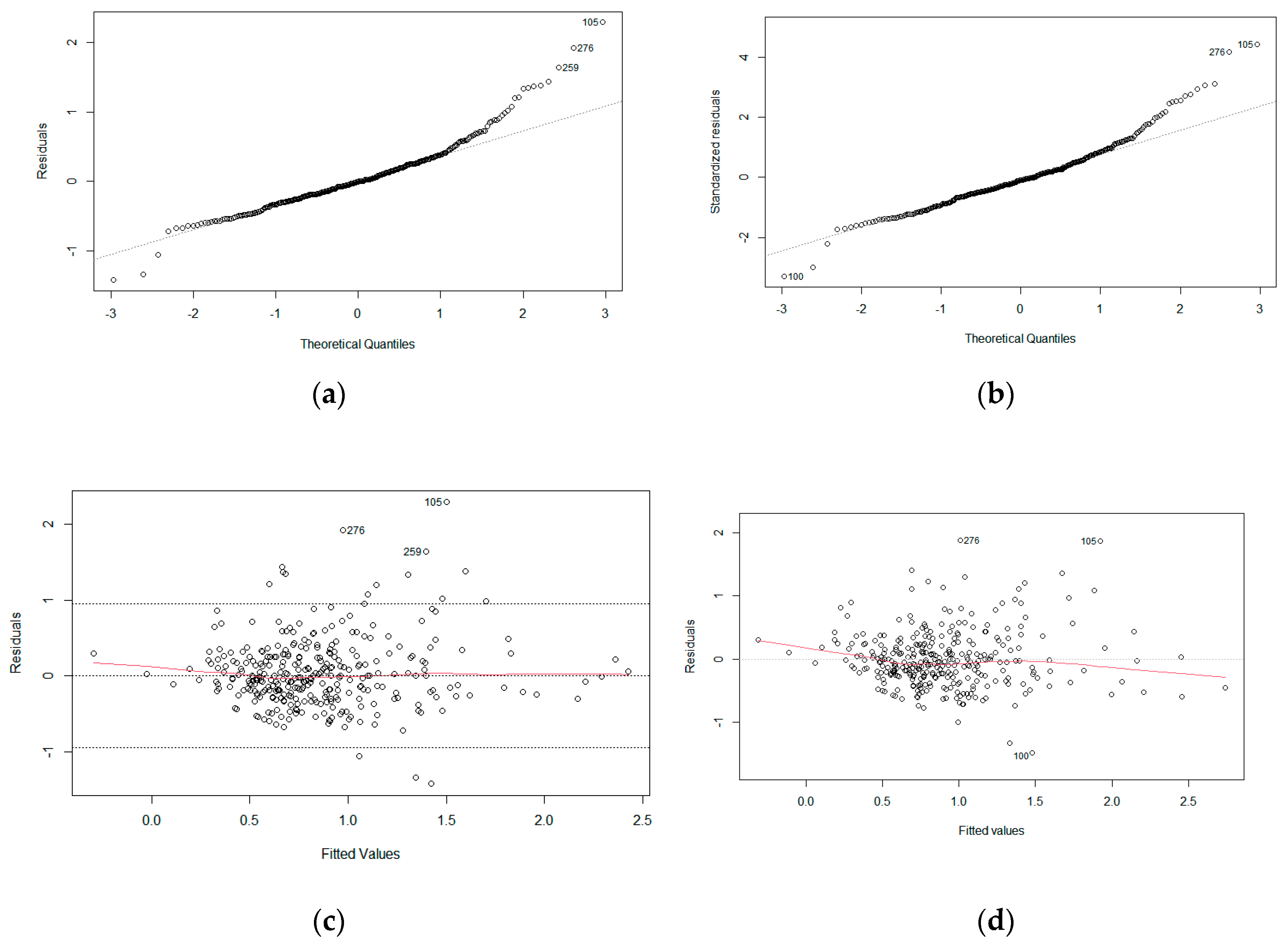

Table 1.
Equivalised total household income (weekly) dataset (code: HIED). Adapted from the Australian Bureau of Statistics.
Table 1.
Equivalised total household income (weekly) dataset (code: HIED). Adapted from the Australian Bureau of Statistics.
| SA2 | 00 | 01 | … | 15 | && | @@ |
|---|---|---|---|---|---|---|
| Nil | $1-$49 | … | $3,000+ | Not Stated | NA | |
| Alexandra Hills | 80 | 84 | … | 52 | 181 | 588 |
| ⁝ | ⁝ | ⁝ | ⁝ | ⁝ | ⁝ | ⁝ |
| Tiarna | 59 | 54 | … | 31 | 138 | 337 |
Table 2.
Input Variable Specifications. Adapted from the Australian Bureau of Statistics [38].
Table 2.
Input Variable Specifications. Adapted from the Australian Bureau of Statistics [38].
| Variable | Numerator | Denominator |
|---|---|---|
| INC_LOW | HIED = 02-05 | HIED = 01-15 |
| INC_HIGH | HIED = 11-15 | HIED = 01-15 |
| ATUNI | AGEP > 14 and TYPP = 50 | AGEP > 14 and TYPP ne &&, VV |
| CERTIFICATE | HEAP = 51 | HEAP ne 001, @@@, VVV, &&& |
| DIPLOMA | HEAP = 4 | HEAP ne 001, @@@, VVV, &&& |
| NOEDU | HEAP = 998 | HEAP ne 001, @@@, VVV, &&& |
| NOYEAR12 | HEAP = 613, 621, 720, 721, 811, 812, 998 and TYPP NE 31, 32, 33 | HEAP ne 001, @@@, VVV, &&& |
| UNEMPLOYED | LFSP = 4-5 | LFSP = 1-5 |
| OCC_DRIVERS | OCCP = 7 | OCCP = 1-8 |
| OCC_LABOUR | OCCP = 8 | OCCP = 1-8 |
| OCC_MANAGER | OCCP = 1 | OCCP = 1-8 |
| OCC_PROF | OCCP = 2 | OCCP = 1-8 |
| OCC_SALES_L | OCCP = 6211, 6212, 6214, 6216, 6219, 6391, 6393, 6394, 6399 | OCCP = 1-8 |
| OCC_SERVICE_L | OCCP = 4211, 4211, 4231, 4232, 4233, 4234, 4311, 4312, 4313, 4314, 4315, 4319, 4421, 4422, 4511, 4514, 4515, 4516, 4517, 4518, 4521, 4522 | OCCP = 1-8 |
| HIGHBED | BEDD = 04-30 and HHCD = 11-32 | BEDD ne &&, @@ and HHCD = 11-32 |
| HIGHMORTGAGE | MRERD = 16-19 | TEND ne &, @ and MRERD ne &&&& and RNTRD ne &&&& |
| LOWRENT | RNTRD = 02-08 | TEND ne &, @ and MRERD ne &&&& and RNTRD ne &&&& |
| OVERCROWD | HOSD = 01-04 | HOSD ne 10, &&, @@ and HHCD = 11-32 |
| NOCAR | VEHD = 00 and HHCD = 11-32 | VEHD ne &&, @@ and HHCD = 11-32 |
| NONET | NEDD = 2 and HHCD = 11-32 | NEDD ne &, @ and HHCD = 11-32 |
| CHILDJOBLESS | LFSF = 16, 17, 19, 25, 26 | LFSF ne 06, 11, 15, 18, 20, 21, 27, @@ |
| DISABILITYU70 | AGEP > 70 and ASSNP = 1 | AGEP < 70 and ASSNP = 1-2 |
| ONEPARENT | FMCF = 3112, 3122, 3212 | FMCF ne @@@@ |
| SEPDIVORCED | MSTP = 3-4 | MSTP = 1-5 |
| Guide: | ||
| [HIED = 02-05] refers to the summation of data satisfying category code 02 to 05 in HED dataset [AGEP > 14 and TYPP ne &&, V.V.] refers to the summation of data satisfying category code greater than 14 in AGEP dataset and category code other than &&, V.V. in TYPP dataset | ||
Table 3.
Robust stepwise regression elimination process.
| Step | Eliminated Variable | Variable Count | RFPE |
|---|---|---|---|
| 0 | NA | 24 | 0.1714 |
| 1 | OCC_LABOUR | 23 | 0.1694 |
| 2 | INC_LOW | 22 | 0.1682 |
| 3 | OCC_SALES_L | 21 | 0.1675 |
| 4 | OVERCROWD | 20 | 0.1668 |
| 5 | NOYEAR12 | 19 | 0.1661 |
| 6 | SEPDIVORCED | 18 | 0.1656 |
| 7 | HIGHMORTGAGE | 17 | 0.1650 |
| 8 | DIPLOMA | 16 | 0.1646 |
| 9 | ONEPARENT | 15 | 0.1645 |
| 10 | NOEDU | 14 | 0.1642 |
| 11 | OCC_PROF | 13 | 0.1640 |
| Scale = 0.381251 | |||
Table 4.
Final Model for Socioeconomic Predictors of Building Fires by Robust Backward Elimination method.
Table 4.
Final Model for Socioeconomic Predictors of Building Fires by Robust Backward Elimination method.
| Variables | Coefficient Est. | Std. Error | t value | F value | (Pr>t) |
|---|---|---|---|---|---|
| (INTERCEPT) | -0.02269 | 0.16582 | -0.137 | - | 0.891243 |
| ATUNI | -1.83339 | 0.72752 | -2.520 | 6.3507 | 0.012223 |
| CERTIFICATE | 1.80594 | 0.63852 | 2.828 | 7.9995 | 0.004976 |
| CHILDJOBLESS | -2.46628 | 0.62832 | -3.925 | 15.4071 | 0.000106 |
| DISABILITYU70 | 5.56711 | 3.47242 | 1.603 | 2.5704 | 0.109875 |
| HIGHBED | -0.50131 | 0.22145 | -2.264 | 5.1243 | 0.024266 |
| INC_HIGH | -0.78460 | 0.41572 | -1.887 | 3.5621 | 0.060023 |
| LOWRENT | 2.00959 | 1.05002 | 1.914 | 3.6628 | 0.056536 |
| NOCAR | 4.93414 | 0.97324 | 5.070 | 25.7027 | 6.77e-07 |
| NONET | 2.20067 | 1.51846 | 1.449 | 2.1004 | 0.148245 |
| OCC_DRIVERS | 0.84838 | 0.60595 | 1.400 | 1.9602 | 0.162462 |
| OCC_MANAGERS | 6.06510 | 1.18788 | 5.106 | 26.0696 | 5.68e-07 |
| OCC_SERVICE_L | -5.28724 | 2.07960 | -2.542 | 6.4639 | 0.011482 |
| UNEMPLOYED | 7.99240 | 2.07421 | 3.853 | 14.8474 | 0.000141 |
| Robust residual standard error: 0.3779 Multiple R-squared: 0.4259, Adjusted R-squared: 0.4024 Convergence in 5 IRWLS iterations | |||||
Table 5.
The RMSE and MAE of models produced by RFPE after 5-fold cross-validation.
| Testing Dataset | Training Dataset | Measurements | |||||
|---|---|---|---|---|---|---|---|
| RMSE | MAE | ||||||
| Train. | Test. | Diff. | Train. | Test. | Diff. | ||
| 1 | 2,3,4,5 | 0.4794 | 0.4272 | 0.0522 | 0.3356 | 0.3150 | 0.0206 |
| 2 | 1,3,4,5 | 0.4618 | 0.4436 | 0.0182 | 0.3217 | 0.3223 | -0.0006 |
| 3 | 1,2,4,5 | 0.4222 | 0.5961 | -0.1739 | 0.3067 | 0.4008 | -0.0941 |
| 4 | 1,2,3,5 | 0.4671 | 0.4264 | 0.0406 | 0.3298 | 0.3291 | 0.0007 |
| 5 | 1,2,3,4 | 0.4512 | 0.5194 | -0.0682 | 0.3120 | 0.3866 | -0.0747 |
| Mean | 0.4563 | 0.4825 | -0.0262 | 0.3211 | 0.3508 | -0.0296 | |
Table 6.
Eliminated variable at every step of the algorithm with AIC criterion.
| Step | Eliminated Variable | Variable Count | AIC |
|---|---|---|---|
| 0 | NA | 24 | -456.72 |
| 1 | SEPDIVORCED | 23 | -458.72 |
| 2 | OCC_PROF | 22 | -460.69 |
| 3 | DIPLOMA | 21 | -462.55 |
| 4 | ATUNI | 20 | - 464.44 |
| 5 | HIGHMORTGAGE | 19 | -466.11 |
| 6 | OCC_SALES_L | 18 | -467.47 |
| 7 | NONET | 17 | -468.79 |
| 8 | OVERCROWD | 16 | -470.24 |
| 9 | OCC_LABOUR | 15 | -471.3 |
| 10 | NOYEAR12 | 14 | -472.3 |
| 11 | ONEPARENT | 13 | -473.03 |
| 12 | INC_LOW | 12 | -474.24 |
Table 7.
Final Model for Socioeconomic Predictors of Building Fires by AIC criterion.
| Variables | Coefficient Est. | Std. Error | t value | F value | (Pr>t) |
|---|---|---|---|---|---|
| (INTERCEPT) | -0.1100 | 0.1873 | -0.587 | - | 0.557377 |
| CERTIFICATE | 3.1137 | 0.6835 | 4.555 | 20.7521 | 7.45e-06 |
| CHILDJOBLESS | -2.4499 | 0.6825 | -3.589 | 12.8829 | 0.000384 |
| DISABILITYU70 | 10.9674 | 3.4643 | 3.166 | 10.0225 | 0.001696 |
| HIGHBED | -1.0020 | 0.2083 | -4.812 | 23.1523 | 2.31e-06 |
| INC_HIGH | -0.9833 | 0.4609 | -2.133 | 4.5508 | 0.033666 |
| LOWRENT | 1.8837 | 1.1387 | 1.654 | 2.7367 | 0.099051 |
| NOCAR | 4.1672 | 1.0614 | 3.926 | 15.4153 | 0.000106 |
| NOEDU | 20.6816 | 6.1309 | 3.373 | 11.3795 | 0.000834 |
| OCC_DRIVERS | 1.5652 | 0.6468 | 2.420 | 5.8565 | 0.016078 |
| OCC_MANAGERS | 7.9097 | 1.2852 | 6.155 | 37.8796 | 2.26e-09 |
| OCC_SERVICE_L | -6.6726 | 2.2015 | -3.031 | 9.1861 | 0.002638 |
| UNEMPLOYED | 5.2595 | 2.3642 | 2.225 | 4.9490 | 0.026805 |
| Residual standard error: 0.4544 on 319 degrees of freedom Multiple R-squared: 0.473, Adjusted R-squared: 0.4532 F-statistic: 23.86 on 12 and 319 DF, p-value: < 2.2e-16 | |||||
Table 8.
Summary of comparative measures of models produced by AIC and RFPE method.
| Measures | RFPE | AIC |
|---|---|---|
| RMSE | 0.4547 | 0.4454 |
| MAE | 0.3254 | 0.3280 |
Table 9.
Summary of comparative measures of models produced by AIC and RFPE after 5-fold cross-validation.
Table 9.
Summary of comparative measures of models produced by AIC and RFPE after 5-fold cross-validation.
| Elimination Criteria | Testing Dataset | Training Dataset | Measurement | |||||
|---|---|---|---|---|---|---|---|---|
| RMSE | MAE | |||||||
| Train. | Test. | Diff. | Train. | Test. | Diff. | |||
| RFPE | 1 | 2,3,4,5 | 0.4794 | 0.4272 | 0.0522 | 0.3356 | 0.3150 | 0.0206 |
| 2 | 1,3,4,5 | 0.4618 | 0.4436 | 0.0182 | 0.3217 | 0.3223 | -0.0006 | |
| 3 | 1,2,4,5 | 0.4222 | 0.5961 | -0.1739 | 0.3067 | 0.4008 | -0.0941 | |
| 4 | 1,2,3,5 | 0.4671 | 0.4264 | 0.0406 | 0.3298 | 0.3291 | 0.0007 | |
| 5 | 1,2,3,4 | 0.4512 | 0.5194 | -0.0682 | 0.3120 | 0.3866 | -0.0747 | |
| Mean | 0.4563 | 0.4825 | -0.0262 | 0.3211 | 0.3508 | -0.0296 | ||
| AIC | 1 | 2,3,4,5 | 0.4516 | 0.4512 | 0.0004 | 0.3365 | 0.3428 | -0.0063 |
| 2 | 1,3,4,5 | 0.4469 | 0.4469 | 6.06e-05 | 0.3338 | 0.3236 | 0.0102 | |
| 3 | 1,2,4,5 | 0.4148 | 0.6054 | -0.1906 | 0.3100 | 0.4156 | -0.1055 | |
| 4 | 1,2,3,5 | 0.4540 | 0.4193 | 0.0347 | 0.3314 | 0.3223 | 0.0091 | |
| 5 | 1,2,3,4 | 0.4382 | 0.5080 | -0.0698 | 0.3221 | 0.3896 | -0.0675 | |
| Mean | 0.4411 | 0.4862 | -0.0451 | 0.3268 | 0.3588 | -0.0320 | ||
Table 10.
Summary of comparative measures of models produced by RFPE, p-value, Adjusted R-squared, BIC and PRESS criteria.
Table 10.
Summary of comparative measures of models produced by RFPE, p-value, Adjusted R-squared, BIC and PRESS criteria.
| Measures | RFPE | p-value | Adj. R-squared | BIC | PRESS |
|---|---|---|---|---|---|
| RMSE | 0.4547 | 0.4582 | 0.4494 | 0.4456 | 0.4472 |
| MAE | 0.3254 | 0.3415 | 0.3456 | 0.3368 | 0.3278 |
Table 11.
Summary of comparative measures of models produced by RFPE, p-value, Adjusted R-squared, BIC and PRESS criteria after 5-fold cross-validation.
Table 11.
Summary of comparative measures of models produced by RFPE, p-value, Adjusted R-squared, BIC and PRESS criteria after 5-fold cross-validation.
| Elimination Criteria | Testing Dataset | Training Dataset | Measurements | |||||
|---|---|---|---|---|---|---|---|---|
| RMSE | MAE | |||||||
| Train. | Test. | Diff. | Train. | Test. | Diff. | |||
| RFPE | 1 | 2,3,4,5 | 0.4794 | 0.4272 | 0.0522 | 0.3356 | 0.3150 | 0.0206 |
| 2 | 1,3,4,5 | 0.4618 | 0.4436 | 0.0182 | 0.3217 | 0.3223 | -0.0006 | |
| 3 | 1,2,4,5 | 0.4222 | 0.5961 | -0.1739 | 0.3067 | 0.4008 | -0.0941 | |
| 4 | 1,2,3,5 | 0.4671 | 0.4264 | 0.0406 | 0.3298 | 0.3291 | 0.0007 | |
| 5 | 1,2,3,4 | 0.4512 | 0.5194 | -0.0682 | 0.3120 | 0.3866 | -0.0747 | |
| Mean | 0.4563 | 0.4825 | -0.0262 | 0.3211 | 0.3508 | -0.0296 | ||
| p-value | 1 | 2,3,4,5 | 0.4858 | 0.4413 | 0.0446 | 0.3515 | 0.3434 | 0.0082 |
| 2 | 1,3,4,5 | 0.5028 | 0.4732 | 0.0295 | 0.3804 | 0.3581 | 0.0223 | |
| 3 | 1,2,4,5 | 0.4664 | 0.6604 | -0.1940 | 0.3540 | 0.4529 | -0.0989 | |
| 4 | 1,2,3,5 | 0.5217 | 0.4353 | 0.0864 | 0.3917 | 0.3251 | 0.0667 | |
| 5 | 1,2,3,4 | 0.4557 | 0.5102 | -0.0545 | 0.3345 | 0.3917 | -0.0572 | |
| Mean | 0.4865 | 0.5041 | -0.0176 | 0.3624 | 0.3742 | -0.0118 | ||
|
Adjusted R-squared |
1 | 2,3,4,5 | 0.4567 | 0.4375 | 0.0192 | 0.3384 | 0.3305 | 0.0079 |
| 2 | 1,3,4,5 | 0.4511 | 0.4482 | 0.0029 | 0.3409 | 0.3240 | 0.0168 | |
| 3 | 1,2,4,5 | 0.4203 | 0.6193 | -0.1990 | 0.3150 | 0.4233 | -0.1083 | |
| 4 | 1,2,3,5 | 0.4624 | 0.4147 | 0.0477 | 0.3350 | 0.3192 | 0.0158 | |
| 5 | 1,2,3,4 | 0.4423 | 0.5215 | -0.0793 | 0.3275 | 0.3987 | -0.0711 | |
| Mean | 0.4466 | 0.4882 | -0.0417 | 0.3314 | 0.3591 | -0.0278 | ||
| BIC | 1 | 2,3,4,5 | 0.4567 | 0.4375 | 0.0192 | 0.3384 | 0.3305 | 0.0079 |
| 2 | 1,3,4,5 | 0.4588 | 0.4485 | 0.0103 | 0.3414 | 0.3309 | 0.0106 | |
| 3 | 1,2,4,5 | 0.4203 | 0.6193 | -0.1990 | 0.3150 | 0.4233 | -0.1083 | |
| 4 | 1,2,3,5 | 0.4672 | 0.4252 | 0.0420 | 0.3399 | 0.3304 | 0.0095 | |
| 5 | 1,2,3,4 | 0.4457 | 0.5631 | -0.1173 | 0.3315 | 0.4245 | -0.0930 | |
| Mean | 0.4497 | 0.4987 | -0.0489 | 0.3332 | 0.3679 | -0.0347 | ||
| PRESS | 1 | 2,3,4,5 | 0.4701 | 0.4369 | 0.0332 | 0.3442 | 0.3318 | 0.0124 |
| 2 | 1,3,4,5 | 0.4494 | 0.4447 | 0.0047 | 0.3313 | 0.3232 | 0.0081 | |
| 3 | 1,2,4,5 | 0.4300 | 0.6234 | -0.1934 | 0.3231 | 0.4261 | -0.1030 | |
| 4 | 1,2,3,5 | 0.4624 | 0.4147 | 0.0477 | 0.3350 | 0.3192 | 0.0158 | |
| 5 | 1,2,3,4 | 0.4457 | 0.5706 | -0.1248 | 0.3256 | 0.4048 | -0.0792 | |
| Mean | 0.4515 | 0.4981 | -0.0465 | 0.3319 | 0.3610 | -0.0292 | ||
Disclaimer/Publisher’s Note: The statements, opinions and data contained in all publications are solely those of the individual author(s) and contributor(s) and not of MDPI and/or the editor(s). MDPI and/or the editor(s) disclaim responsibility for any injury to people or property resulting from any ideas, methods, instructions or products referred to in the content. |
© 2023 by the authors. Licensee MDPI, Basel, Switzerland. This article is an open access article distributed under the terms and conditions of the Creative Commons Attribution (CC BY) license (http://creativecommons.org/licenses/by/4.0/).
Copyright: This open access article is published under a Creative Commons CC BY 4.0 license, which permit the free download, distribution, and reuse, provided that the author and preprint are cited in any reuse.


