
Submitted:
15 February 2023
Posted:
20 February 2023
You are already at the latest version
Abstract
Ecological niche models have become exceptionally important, since their results allow to un-derstand many aspects related to the biology of the species being studied, even understanding its evolutionary relationships or their response to past or future projections. In this research, models were prepared to create climatic surfaces so as to produce bioclimatic layers based on the mete-orological data of the south of Peru. Temperature and precipitation data from 119 stations were obtained and homogenized. Then, using geographic and orographic covariates, models were prepared so as to obtain climatic surfaces of maximum and minimum temperature, and precipi-tation. The produced layers were evaluated through root-mean-square deviation (RMSD), mean absolute deviation of error (MAD) and goodness of fit (R2), and they were compared to other models for the area. Finally, the 19 bioclimatic surfaces were created. The results show general patterns for temperature and precipitation, some of them being particular. The climatic layers produced showed acceptable values for RMSD, MAD and R2. Comparison with other models shows statistically significant differences. Both the climatic and the produced bioclimatic surfaces were entered into a database for free access. Finally, comments are made on the importance and application of the bioclimatic layers produced here.
Keywords:
interpolation
; SDM
; ENM
; precipitation
; climatic surfaces
1. Introduction
The use of bioclimatic models to study the ecological niche of species has been consolidated as a research field, since its application can contribute to knowing the potential distribution of living organisms, bringing us closer to macroecology [1,2]. The use of climate models related to the distribution of species can be applied to learn about habitat changes from various points of view (conservation of species, dispersion of disease vectors, colonization of organisms foreign to new ecosystems, effects of climate change, etc.) [3,4,5], which contributes to biodiversity management, or making appropriate decisions for the sustainability of ecosystems. On the other hand, although bioclimatic models are used for the present time, they can also be projected to the past (for instance, [3,6,7]), or to the future (for instance, [8,9]), so that they can be related to other aspects, providing information to understand certain phylogenetic, biogeographic or adaptability aspects of the treated species.
The information that determines the distribution of an organism is provided by its environmental tolerances, intrinsic relationships, and dispersion potential [10]; however, the last two are somehow hard to be known and, therefore, the use of only environmental variables has become extensive [11]. Information such as precipitation, maximum temperature, minimum temperature, humidity, solar radiation, evaporation, among other variables, help to determine the distribution of an organism and to understand biological and evolutionary aspects [5]. However, much of the information collected with specialized instruments is limited to only some variables (which is common in meteorological stations of a certain age), so that some of the environmental variations of certain localities are unknown [12]. Nevertheless, the production of climate models, in relation to some topographic covariates, can help to fill information gaps, which is possible using interpolations through the specific knowledge of variables close to the area and even the use of some satellite indices to correlate climate events [12,13,14,15,16,17,18].
At present, there are worldwide (or global) bioclimatic models that have been calculated with data from ground-based meteorological stations [15], satellite information [19,20] or a combination of both [14]. In some cases, comparisons were made between models generated with ground and satellite information, showing that the latter has a better performance, although it should be applied to sectors with low density of ground stations (such as tropical rainforests); in addition, for sectors with many topographic irregularities, data validation should be performed [21,22,23]. Regional bioclimatic models were produced in order to improve the local climate representativeness, taking into consideration a greater amount of climate information, so as to achieve a more “realistic” representation of the local climatic variability and, therefore, the ecological niche of the species [12,24,25]. Usually, the maximum resolution of bioclimatic models is found at approximately 1 km2 of the surface, but can also be found at lower resolutions [3,14,19].
In the case of Peru, and specifically the southern area (Arequipa, Moquegua, and Tacna), no specific climate surfaces have been developed. However, the National Meteorology and Hydrology Service (SENAMHI) has disclosed climate information contained in raster layers with a resolution of 5 km2 for Peru. This information, obtained from the combined analysis of data from meteorological and satellite stations [26], though no topographic covariates were used, represents a breakthrough for obtaining these data in Peru. On the other hand, the so-called “global” climate models, although representing the south of Peru, can be considerably biased given the scarce data used for their interpolation, and even the topographic complexity of the area makes the data presented by the “global” climate models even more variable [4,13,14,19,27,28].
Finally, given the current knowledge in the application of the bioclimatic models and the lacking thereof in our environment, we need to understand more “accurately” the climate variability in the south of Peru. Preparing species niche models with the right information will guarantee that their predictions are optimally made and reflect the environmental suitability of the species. Producing ecological niche models that reflect the local reality and that are based on reliable climate information will guarantee better decision making in terms of conservation or even health and environmental safety. Therefore, this study seeks to produce surfaces of maximum and minimum temperature, precipitation, and bioclimatic layers of the southern area of Peru for the conservation of biodiversity.
2. Materials and Methods
2.1. Area of Study
It includes the departments of Arequipa, Moquegua, and Tacna, from approximately 14° 39′ to 18° 18′ south latitude, and from 0 to 6427 m.a.s.l. (Figure 1). The topography is variable because the coast holds the old coastal mountain range, the peaks of which do not exceed 1500 m.a.s.l.; immediately after, to the east, there is the desert coastal plateau, characterized by extensive hyperarid plains, which sometimes reach 2500 m.a.s.l., and which are delimited by the foothills of the volcanic mountain range, the peaks of which easily surpass 5500 m.a.s.l. Finally, crossing the volcanic mountain range, there is the so-called Andean plateau or altiplano, which is crossed by the deepest canyons on the planet and at the bottom of which run turbulent rivers that flow into the Pacific Ocean.
The climate is typically dry, with only two distinguishable seasons: Wet and dry. The areas corresponding to the foothills of the volcanic mountain range and the altiplano have rainfall during the austral summer, but are dry during the rest of the year. On the other hand, in the coastal area, the wet season happens during the winter and the humidity coming from the Pacific Ocean enters the continent as stratocumulus clouds trapped in the spurs of the coastal mountain range or, in some cases, in the last foothills of the Andes (including the valleys that end in the sea). Lastly, the area of the desert plateau receives almost no precipitation and has high solar radiation throughout the year.
2.1. Collecting climate information
The climate information was collected from the National Meteorology and Hydrology Service (SENAMHI) (https://www.senamhi.gob.pe/?&p=descarga-datos-hidrometeorologicos), the National Water Authority (ANA) (https://snirh.ana.gob.pe/ObservatorioSNIRH/), Explorador Climático (https://explorador.cr2.cl/) and privately owned meteorological stations. The data collected were: Maximum temperature, minimum temperature, and precipitation, covering from 1964 to 2018. On the other hand, since not all the stations have the previously indicated time interval, the information thereof was taken into account that they provide at least one full year of records [24]. Given that the climate information in the area is poor, it is necessary to consider that having more records will help to better represent the climate variability of the area, improving the recreation of the produced models [12,24]. Finally, additional information was collected from stations located close to the limits established for the area of study so as to avoid the edge effect [24].
For the coastal area (lomas communities), 20 “virtual” meteorological stations were used and randomly located within the lomas ecosystems [29]. The monthly values of the “virtual” stations were assigned taking into consideration the ratio between the monthly precipitation of actual stations and the NDVI (Normalized Difference Vegetation Index) values of the lomas ecosystems. The NDVI values were obtained from the MOD13Q1 V6 product corresponding to the MODIS satellite, which has a spatial resolution of 250 m every 16 days. This product was selected because of its sensitivity in the desert of western South America [30]. In fact, it is the most suitable, since its products mask clouds, dense aerosols and cloud shadows [30,31]. Images were obtained from https://earthexplorer.usgs.gov, covering all the months of the year, from 2000 to 2018. The images were processed in QGIS v.3.26.2 [32] and monthly NDVI averages were obtained for an 18-year range. Once obtained, the averaged surfaces for each month were cut with a shapefile corresponding to the lomas ecosystem [29]. The localization of the weather stations located in the lomas (Atiquipa and Sama Grande stations) was plotted on the monthly NDVI surfaces, and the corresponding pixel values were extracted. The monthly precipitation and NDVI values extracted from the stations were respectively averaged. The localization of the “virtual” stations was plotted and the respective monthly NDVI was extracted. Finally, the precipitation values of the “virtual” stations were found by proportionally and directly relating the known precipitation according to the corresponding NDVI, all this with respect to the NDVI extracted for the localization of the “virtual” station. The following mathematical relationship was used:
where:
= Unknown monthly precipitation (mm).
= Monthly precipitation of the real station (mm).
= NDVI extracted for the virtual station.
= NDVI extracted for the real station.
It should be noted that the calculation is independent for each monthly NDVI value obtained.
2.2. Georeferencing weather stations
The georeferencing of stations was initially performed with information contained in the SENAMHI and ANA websites. However, some errors (wrong localization) were undetected and, considering that some stations were rather old, it was decided to verify their position taking some considerations into account. First, for the stations that are currently operating, localization was correct in most cases and only a small adjustment was made. Second, localization for old stations was set towards the central square of the village indicated in their information sheets. All georeferencing was performed with high-resolution satellite images (0.3 m) contained in Google Earth Pro v3.4.
2.3. Treatment of climate information
The climate information from every station was stored in spreadsheets. Six daily series of information were obtained and preliminarily treated with filters to eliminate extreme or atypical values. Then, using pivot tables, the data sequence, information gaps, and monthly averages for each year on record (temperatures in °C) or the total sum of monthly values for each year (precipitation in mm) were verified. After verifying the data, homogenization and autocompletion (analysis to detect and correct atypical data, as well as to complete missing data through correlation taking into account latitude, longitude and altitude) were performed using the Climatol v3.1.2 package (https://github.com/cran/climatol) [33] installed in RStudio [34].
2.4. Covariates, modeling of climatic surfaces and validation
We used an ASTER digital elevation model (DEM) from the Ministry of the Environment of Peru (https://geoservidor.minam.gob.pe/), with a resolution of 0.0083°, equivalent to approximately 1 km2 (30 seconds), with a WGS84 reference system of longitude, latitude and datum. Also, as recommended some authors [13,14,24,35], given the topography of the area, the covariates used were slope, orientation, cloud cover, additionally including the Topographic Wetness Index (TWI) and the distance to the coast. Slope and orientation were obtained using the DEM, through the modeling implemented in QGIS v3.26.2 [32]. The TWI was obtained using the methodology of [36] and [37]. Cloud cover data were obtained from http://www.earthenv.org/cloud [35]. Finally, the distance to the coast was obtained from https://oceancolor.gsfc.nasa.gov/docs/distfromcoast.
The climatic surface were modeled with ANUSPLIN 4.4 [38]. ANUSPLIN uses data from the different covariates through the thin plate smoothing spline algorithm, producing surfaces with smooth values and without drastic changes. As for the evaluation of the reliability of the produced surfaces, and given the number of meteorological stations, it was decided to use a 10-fold (k-fold) cross-validation. To that effect, first, all the stations were randomly arranged and, then, a percentage thereof was removed so as to finally obtain 10 data lists where a 20% of information was missing (it should be noted that this was done independently, both for maximum and minimum temperature, and for precipitation). Then, the models were produced with each information list obtained; 10 iterations were applied, choosing among them that which presented the lowest value of residues and showed a linear behavior thereof. After choosing the corresponding surfaces, these were evaluated with the data of the stations that were left out of the model, using the root mean square deviation of cross-validation (RMSEcv). Finally, the surfaces produced for each month (corresponding to the 10 folds made) were averaged. A similar process was performed for the RMSEcv. Additionally, the mean absolute deviation of error (MAD) was calculated.
2.5. Comparison with other climatic surfaces for the area of study
The produced surfaces, i.e., accumulated annual precipitation and mean temperatures, were compared to those of WorldClim 2 and CHELSA [14,19] (they were not compared to [20] because their layers had a lower resolution and, instead of using precipitation, they used specific humidity). In this case, in order to better understand the area of study regarding precipitation, it was subdivided into two areas. The first included the coastal area, i.e., from 0 to 1500 m.a.s.l., and the second included the Andean area, above 1500 m.a.s.l. In order to obtain rainfall data, 2000 random points were superimposed in each area and the corresponding information was extracted at them. As for mean temperature, 4000 random points in total were used in the area of study. The Kruskal–Wallis statistical test was used with a 95% level of reliability, so as to detect potential significant differences.
2.6. Production of bioclimatic layers
The 19 bioclimatic surfaces were created from the produced climatic surfaces (12 of maximum temperature, 12 of minimum temperature, and 12 of precipitation) in [34] and using the Dismo package [39]. All of them were developed according to WorldClim and ANUNCLIM [14,15,40]. The mathematical details to create each of the surfaces can be found in [19,40].
3. Results
3.1. Climate information
Information from 118 stations was used. Eighty provided information on precipitation and temperature, 30 on precipitation only and eight on temperature only (Figure 2).
Mean temperature behavior shows that the warm months are January, February, and March (corresponding to the austral summer), while the cold months are June, July, and August (corresponding to winter). The highest temperature is recorded in February (24.8 °C) and the lowest in July (-0.6 °C) (Figure 3A). On the other hand, an individual analysis of the maximum and minimum temperatures shows that the average maximum temperatures in the areas under 1500 m.a.s.l. (coast, desert plateau, and arid valleys) take place in the summer months, February being the warmest with an average of 27.4 °C, while the colder months are June, July, and August, July recording the lowest values with an average of 20.8 °C. As for the areas above 1500 m.a.s.l. (western slopes and altiplano), the warmer months are September, October, and November, the warmest being November with an average of 20.1 °C, while the colder months were June and July, the latter being the coldest with an average of 18 °C. Regarding the minimum temperature, a single pattern is observed, the warmer months corresponding to summer and February being the warmest with an average of 9.7 °C, while the lower values are recorded during the winter, July being the coldest with an average of 3.8 °C.
Precipitation in the coastal area predominantly occurs during the winter months, i.e., in the months of July, August, and September, the latter presenting the highest values (an average of 1.8 mm). It is worth noting that the stations close to hill ecosystems, such as Aquitipa (Arequipa) and Sama Grande (Tacna), have the highest precipitation values (13 and 7.1 mm, respectively). March, April, and May are the driest months in the coastal area, April being the lowest with 0.02 mm (Figure 3B).
In the highlands (above 1500 m.a.s.l.) the rainy season corresponds to the summer months of January, February, March, including December. In contrast, the rest of the year, from April to November, are months with little precipitation. In the Andean area, the month with the most precipitation is February (with a mean of 89 mm). On the other hand, July is the “driest” month, with a mean precipitation of 1 mm (Figure 3C).
3.2. Modeling of climatic surfaces
Thirty-six climate surfaces per month were obtained, corresponding to maximum temperature (12 surfaces), minimum temperature (12 surfaces) and precipitation (12 surfaces) (Figure 4). As for their average maximum temperature values, it can be noted that the warmer months are November and December, November being the one with the highest value. For the same variable, June, July, and August were the colder months, July being the coldest (Table 1).
Thirty-six thousand surfaces were produced, which, after the evaluations and procedures performed, were reduced to 36 corresponding to maximum temperature (12 surfaces), minimum temperature (12 surfaces) and precipitation (12 surfaces) (Figure 4). As for their average maximum temperature values (Figure 5), it can be noted that the warmer months are November and December, November being the one with the highest value. For the same variable, June, July, and August were the colder months, July being the coldest (Table 1).
Regarding the minimum temperature, the warmer months were January, February, and March, February being the warmest. On the other hand, June, July, and August were the months with lower temperatures, July recording the lowest value (Table 2).
As for precipitation, January, February, and March had the higher values, January and February having the highest with a mean of 65.0 mm and 67.3 mm, respectively. On the other hand, the months with the lower values were May, June, and July, the driest being June, with a mean of 2.2 mm, and July, with a mean of 2.0 mm.
On the other hand, the patterns of the produced surfaces in terms of altitude, ocean–inland distance and orientation are recognizable (Figure 6). The temperature surfaces are clearly closely related to altitude (Figure 6A,B) in that it lowers with altitude, and there is no marked relation to the ocean–inland distance and orientation. Precipitation (Figure 6C) shows a certain relation to altitude, although it is only marked for the western part and the vicinity of the great mountains (precipitation increases with altitude). However, the greater the ocean–inland distance (which goes hand in hand with orientation), precipitation also increases. It should be noted that maximum temperature and precipitation in the coastal area have particularities. It can be seen that the maximum temperature notoriously decreases in the area of formation of lomas and then increases (which does not happen with the minimum temperature). Precipitation in the coastal area increases (almost matching rain values around 40 km inland) and then decreases to very low values.
3.3. Validation of temperature and precipitation surfaces.
Values were obtained for each test (Table 4). The RMSEcv range for maximum temperature is between 1.4 and 1.7, with an average of 1.5. In the case of MAD, values are between 1.0 and 1.3, with a mean of 1.1.
The RMSEcv range for minimum temperature was between 0.58 and 1.24, the average being 1.2. The MAD interval was 0.6 to 1.2, with a mean of 0.9.
The RMSEcv for precipitation had a 1.3 to 12.2 interval, the mean being 5.8. The MAD interval was 1.0 to 8.6, with a mean of 4.0.
3.4. Comparison with other surfaces and production of bioclimatic layers
In general, the obtained surfaces indicate more precipitation and higher temperature values compared to those of [6] and [12]. However, in the case of coastal precipitation, on average, an “intermediate” value was obtained compared to [6] and [12]. This was not the case for the Andean Area, where there was a higher value (Table 5). After applying the corresponding tests, it was found that there are statistical differences for the evaluated surfaces. In some cases, there were highly significant differences (p < 0.01). Globally, it can be indicated that the surfaces produced herein are statistically closer to those of [6] (Figure 5), since they presented significant differences (p < 0.05) in two cases.
In general, the obtained surfaces indicate more precipitation and higher temperature values compared to those of [14] and [19]. However, in the case of coastal precipitation, on average, an “intermediate” value was obtained compared to [14] and [19]. This was not the case for the Andean Area, where there was a higher value (Table 5). After applying the corresponding tests, it was found that there are statistical differences for the evaluated surfaces. In some cases, there were highly significant differences (p < 0.01). Globally, it can be indicated that the surfaces produced herein are statistically closer to those of [14] (Figure 7), since temperature did not show a statistical difference and was merely significant regarding Andean precipitation.
Finally, the 19 bioclimatic layers were produced from the 36 climatic surfaces, and are available for free in Zenodo, at: https://zenodo.org/record/6975996#.YvJpcXbMLtR (the 36 produced surfaces are also available for consultation at the same link). The denomination of each is mentioned below: bio1 = mean annual temperature (°C), bio2 = mean daytime range (°C), bio3 = isothermality, bio4 = temperature seasonality (standard deviation), bio5 = maximum temperature of the warmest month (°C), bio6 = minimum temperature of the coldest month (°C), bio7 = annual temperature range (°C), bio8 = mean temperature of the wettest quarter (°C), bio9 = mean temperature of the driest quarter (°C), bio10 = mean temperature of the warmest quarter (°C), bio11 = mean temperature of the coldest quarter (°C), bio12 = annual precipitation (mm/year), bio13 = precipitation of the rainiest month (mm/month), bio14 = precipitation of the driest month (mm/month), bio15 = precipitation seasonality (coefficient of variation), bio16 = precipitation of the wettest quarter (mm/quarter), bio17 = precipitation of the driest quarter (mm/quarter), bio18 = precipitation of the warmest quarter (mm/quarter), bio19 = precipitation of the coldest quarter (mm/quarter).
4. Discussion
4.1. Patterns of the climatic information obtained
As already known, temperature shows some patterns, like its decrease related to the a higher topographic altitude [41] or higher values during the summer season or a drop at higher geographical latitudes [42,43]. The analysis of the temperature data included herein shows the common patterns of temperature variation based on altitude; however, an analysis per season shows that the maximum temperature, unlike the minimum (with high values during the summer and low values during the winter), in the Andean areas (> 1500 m.a.s.l.) takes place in September, October, and November. The aforementioned pattern for maximum temperature was also observed by [44], also indicating that the month with the highest values is November. On the other hand, the reason why September, October, and November are the warmer months in the Andean area would be related to seasonal rainfall. The summer months (including part of December) in the Andean area correspond to the rainy season; therefore, the presence of cloudy masses is much more frequent, thus limiting solar radiation towards the ground surface. This “shadow” created by the clouds, together with the winds created by low pressure, would be responsible for lower maximum temperatures during the summer months. It is worth noting that the variation of the maximum temperature in the Andean areas is not very sharp throughout the year. Like [42], this research shows that this variation is around 2 °C. As for the temperature and longitude relation, as [42] and [45] indicate, it decreases from north to south, but the maximum temperature is sometimes contradictory. In these cases, the location of the station is worth noting; e.g., if it is located in plains or inside valleys. Topographic features model some temperature and precipitation characteristics [13], which, in turn, would potentially interact with wind speed and direction. In the case of valleys, a higher temperature could be caused by the limited movement of air masses.
Precipitation in our environment determines seasons throughout the year, i.e., there are only two seasons: Wet and dry [27,30,31]. As for patterns of precipitation, the latter seems to be related to altitude; however, it is possible to find a certain idiosyncrasy in it [12]. The general precipitation patterns for the western Andes of Peru indicate that precipitation increases with altitude [30] and decreases from north to south [27]; here, however, we will analyze the coastal and Andean areas, specifically. The coastal area of Peru is influenced by three factors defining its wet season: The Humboldt current, the trade winds and the thermal inversion layer in the lower troposphere [30,32], which, during the austral winter, produce very fine rain known as drizzle or misty rain that comes from the stratocumulus clouds and does not go higher than 1000 m.a.s.l. [30,33]. Based on what was obtained, precipitation in the stations located close to the coast is scarce and it increases in those located further inland, where there are hill ecosystems (precipitation occurs even inside the valleys). Probably, the increased precipitation is caused by the clouds “compressing” and producing rain when bumping into the western areas of the coastal mountain range. It is worth noting that the regular wet periods occur during winter. Nevertheless, in December, January, and February there is also a fair amount of precipitation that is due to ENSO events, when the Humboldt current debilitates and, therefore, the ocean becomes warmer, causing heavy rains [32]. As for the Andes, the rainy season is quite noticeable, being limited to summer. Rainfall in the Andean area is produced by geographic and physical factors, the most outstanding of which are the Intertropical Convergence Zone (ITCZ) and the Amazon basin [27,30], which regulate precipitation, decreasing from north to south and from east to west (the latter being related to altitude). All the aforementioned patterns are visible for the area of study, where the higher the elevation, the greater the amount of precipitation (the reference being the constant geographic longitude), while the northern area of Arequipa receives the most precipitation, unlike Tacna (this, considering the same altitude).
Precipitation in our environment determines seasons throughout the year, i.e., there are only two seasons: Wet and dry [42,45,46]. As for patterns of precipitation, the latter seems to be related to altitude; however, it is possible to find a certain idiosyncrasy in it [19]. The general precipitation patterns for the western Andes of Peru indicate that precipitation increases with altitude [45] and decreases from north to south [42]; here, however, we will analyze the coastal and Andean areas, specifically. The coastal area of Peru is influenced by three factors defining its wet season: The Humboldt current, the trade winds and the thermal inversion layer in the lower troposphere [45,47], which, during the austral winter, produce very fine rain known as drizzle or misty rain that comes from the stratocumulus clouds and does not go higher than 1000 m.a.s.l. [45,48]. Based on what was obtained, precipitation in the stations located close to the coast is scarce and it increases in those located further inland, where there are lomas ecosystems (precipitation occurs even inside the valleys). Probably, the increased precipitation is caused by the clouds “compressing” and producing rain when bumping into the western areas of the coastal mountain range. It is worth noting that the regular wet periods occur during winter. Nevertheless, in December, January, and February there is also a fair amount of precipitation that is due to ENSO events, when the Humboldt current debilitates and, therefore, the ocean becomes warmer, causing heavy rains [47]. As for the Andes, the rainy season is quite noticeable, being limited to summer. Rainfall in the Andean area is produced by geographic and physical factors, the most outstanding of which are the Intertropical Convergence Zone (ITCZ) and the Amazon basin [42,45], which regulate precipitation, decreasing from north to south and from east to west (the latter being related to altitude). All the aforementioned patterns are visible for the area of study, where the higher the elevation, the greater the amount of precipitation (the reference being the constant geographic longitude), while the northern area of Arequipa receives the most precipitation, unlike Tacna (this, considering the same altitude).
4.2. Modeling of climatic surfaces and validation
An important aspect to be taken into consideration in modeling is the representativeness of the area, i.e., the quality, quantity and, in this case, the correct geographical position of the input data to perform the interpolations. Some of the produced models use only information from weather stations, satellites or a combination of both [12,14,15,19,20,24]. In tropical countries, the problem of the lack of climate information, either due to the lack of meteorological stations, to the difficult access to information or to incomplete records is highlighted [15,27,28,48]. In this sense, it is possible that the models produced by other authors for the area of study of this research will not properly reflect the climate reality, because only a few ground stations were used or because data were mainly collected by satellite [14,15,19,20], with biases related to topographic complexity and to the density of meteorological stations [27,48]. For this case, the use of as much ground-based climate data available, considering the recommendations by Cuervo-Robayo [24], allowed to obtain “truer” surfaces, better reflecting the temperature and precipitation patterns. It should be noted that the coastal area, unlike the Andean area, has fewer meteorological stations (27% of the total) and that most of them are located near the coast. It is known that the coastal area of Peru has peculiar weather characteristics, with drizzle during the winter, which intensifies inland, towards the windward side of the lomas, creating the lomas ecosystems [42,49]. As previously indicated, the meteorological stations for this area are close to the coast and only two are close to the lomas ecosystems (Atiquipa station, in Arequipa, and Sama Grande, in Tacna).
Given the peculiarities of the lomas ecosystems, and in order to better represent them in the bioclimatic models, it was decided to produce “virtual” stations in the sense that they would have correlated information between the real weather stations (Atiquipa and Sama Grande) and the NDVI index, somehow covering the information “gaps”. The NDVI index, as such, represents health and vegetation cover; therefore, in natural situations, this index is mainly influenced by the amount of moisture in the soil [50,51] and, therefore, of precipitation. In fact, the NDVI-precipitation relation has already been written about, making it clear that they are closely correlated [52,53,54]; although temperature is also related [55,56,57], it seems that, in places where thermal fluctuation is not very wide, this variable does not play a preponderant role [57]. On the other hand, it is also mentioned that the NDVI response, timewise, depends on the nature of rainfall [57]. Thus, in areas where the wet season is sudden, there will be a lack of synchronization between precipitation and NDVI. In turn, in places with a progressive increase of humidity, NDVI peaks and precipitation will be quite close. It should also be noted that, in areas with a marked seasonality, the NDVI-precipitation relation is also close [57]. Then, taking into account the characteristics of precipitation in the formations known as Lomas, it evidently is the marked seasonality and a progressive appearance of vegetation [30,49,58]. In this research, apparently the “virtual” stations created based on the NDVI and precipitation values from real stations was satisfactory, since it shows very significant differences compared to other models. Also, the areas predicted by the model almost perfectly match the lomas vegetation maps [29,30]. In fact, the results show how precipitation occurs in certain sectors of the coastal mountain range (at a certain altitude, slope and orientation), recalling that these ecosystems are specific oases of life surrounded by one of the driest deserts in the world [59]. Anyhow, this is just an applicable solution for these particular ecosystems with closely related climate and a vegetation [60]. Although the performed mathematical operations seem simple, they are a way towards a solution regarding lack of information in the lomas ecosystems. Though in the coastal area of southern Peru there are weather stations which are very close to the coast, these do not reflect the precipitation occurring a few kilometers inland, in the lomas ecosystems. Even during the ENSO (El Niño-Southern Oscillation) events, in stations located close to the coast, precipitation is considerably lower compared to that in the lomas [61]. The veracity of the values found for the “virtual” stations could not be verified here, since the only two stations present in these ecosystems were used for data generation. However, the intention here is that the precipitation conditions in these unique ecosystems are adequately reflected, since other global models only show “flat” values or precipitation mostly restricted to the coastal valleys. The lomas ecosystems are unique in the world, the greatest number of endemic species being found towards the south of Peru [62]. Thus, for a good representation of the niche and distribution models of the species, it is necessary to show them as close as possible to what happens in reality. Further studies are needed to understand the relationship between precipitation and NDVI in lomas ecosystems.
The use of geographic (latitude and longitude) and topographic covariates is common in the modeling of climatic surfaces [14,15,24]. Nevertheless, some others also consider the use of other covariates, such as the cloud cover or the distance from ocean coastline to inland [13,14,63]. Generally, the most used covariate in modeling is altitude [14,15,24] and it is closely related to temperature variations [64]. On the other hand, precipitation, in very broad terms, can show a relation with altitude [45]. However, locally, it is idiosyncratic [19] and will depend on other factors, such as wind currents, topography and the diurnal cycle of solar radiation, these being the most complex in mountain areas [13,28]. In this case, as recommended by some authors [13,24] and considering the topographic complexity, slope, land orientation, TWI, distance to the coast, and cloud cover, were used for modeling, besides altitude, producing good results. In fact, towards the coastal area, where other surfaces show a poor representativeness of precipitation in lomas ecosystems, here they are clearly shown to occur towards the western slopes of the hills (windward).
The use of parameters to measure errors in models is common and necessary, because these parameters indicate de degree of bias or the difference between data collected on site and data interpolated by some model [65,66]. On the other hand, the use of validation values is common to verify the interpolated results in climatic layers with real values collected on site [12,14,24,67]. In this case, a k-fold cross-validation was used, since the reduced amount of available data made it difficult to take a certain percentage for a single training and test [68], which is why it was decided to perform 10-folds with random data and produce models with each of the “sets” of data obtained, finally evaluating the surfaces obtained through the RMSEcv. According to RMSEcv and MAD, the precision of the produced models is adequate and presents relatively low values. Nevertheless, there are some considerations regarding the interpolated variables. Regarding temperature, the RMSEcv and MAD values are higher for the maximum temperature, which indicates more variability, and this is reasonable since the maximum temperature could be influenced by different factors (as explained above), while the minimum temperature is more homogeneous and responds to seasonality [42]. Precipitation, unlike temperature (maximum and minimum) has slightly higher values for RMSEcv and MAD, a pattern also observed in [14,24]. As mentioned before, precipitation is idiosyncratic, with different patterns according to the combination of different factors [28]. This is why the variability of the precipitation models is somewhat high, even more so in places with a complex topography and a poor number of meteorological stations [14]. In this sense, probably for this study, integrating the use of covariates related to topography, humidity and the use of the largest amount of data from meteorological stations favored the low RMSEcv and MAD values. Finally, it is worth noting that the higher RMSEcv and MAD values related to precipitation were obtained in the months of the wet season in the coast (winter) and the Andes (summer), showing once more that it is during these periods when the most variations take place according to the precipitation patterns of each place.
4.3. Comparison with other models produced for the area of study
Statistically, the models produced throughout this research are different from those prepared for the same area, this is, WorldClim and CHELSA [14,19]. The data from the produced layers present highly-significant differences with regard to the CHELSA layers. It is likely that the data obtained for CHELSA [19], satellite-obtained, do not accurately show the temperature and precipitation patterns for the area of study. Usually, specific algorithms related to cloud cover and altitude are used to calculate climate patterns from satellite images, taking into account the analysis of the infrared spectrum in terms of temperature. In this sense, this being a “calculated” process, it needs to be validated with instruments located on the ground, even more so in areas with a complex topography [23]. When compared to WorldClim [14], significant differences were found for Andean precipitation and temperature, and highly significant differences with regard to coastal precipitation. The fact that [14] have obtained more approximate values than those presented here is probably related to the origin of the data, since the authors refer that they collected them from different sources. As for precipitation in the coastal area, the WorldClim and CHELSA models presented highly significant differences compared to the one presented here. This is probably due to the fact that the models produced in this work integrated real and “virtual” values for precipitation in the lomas sectors, which is not very well reflected in [14,19]; in fact, in [14], which is basing its data on [15], it can be observed that no meteorological station is present in the lomas sectors of southern Peru.
4.4. Expectations about the use of bioclimatic layers
The purpose of the produced 19 bioclimatic layers is to provide support for the conservation of flora and fauna species distributed in the departments of Arequipa, Moquegua, and Tacna. Having data that are more representative of the climatic reality of this area will guarantee the production of ecological niche models closer to reality, better outlining the environmental requirements of the potentially studied species, and this not only for endemic species, but also for “problem” species (for example, introduced or parasitic species), or even to detect evolutionary relationships, through the concept of niche conservatism. On the other hand, the surfaces produced here could also be used, for instance, to evaluate the historical biogeography of the species or how climate change could affect them (this, through models projected to the past or to the future, considering the processes or methodologies applied to obtain them). The modeling of the ecological niche (ENM) of the species with layers that are more similar to the climatic reality will allow us to better know the ideal environmental conditions for the species, and, with this, after its projection in the geographic space, we will be able to obtain, in a more approximate way, its geographic and potential distribution (SDM). Finally, it is expected that his work is a source of inspiration to better recreate the environmental and bioclimatic space of Peru, since, as we know, our territory, having a complex topography, needs on-site data for a better climatic representation of its surface and, thus, better understand the ecoclimatic requirements of its species.
5. Conclusions
The analyzed meteorological data present a 54-year amplitude, covering from 1964 to 2018. The patterns obtained regarding the variation of temperature and precipitation are as expected, i.e., that temperature presents an inverse ratio to altitude, a direct ratio to geographic latitude, and values are higher during the summer and lower during the winter. On the other hand, precipitation is idiosyncratic. However, it follows general patterns, which indicate a decrease from north to south and an increase from west to east, which is also related to the increase in altitude. Regarding some specific characteristics, the maximum, minimum and mean temperatures in the coastal and Andean areas are partially as expected, since, in the Andean area, the maximum temperature reaches its highest values in September, October, and November. As for precipitation, in the coastal area, precipitation appears during the winter, while in the Andean area it occurs during the summer. With the climate data, 36 high-resolution climatic surfaces were modeled (12 for maximum temperature, 12 for minimum temperature, and 12 for precipitation, each corresponding to a month of the year), which, according to the RMSEcv and MAD data, are optimal compared to the original data. The comparison between the models produced here and those produced by the other authors, who worked in the same area of study, shows significant and highly significant differences, a greater difference with the precipitation in the coastal area being specified. Finally, based on the climatic surfaces, 19 high-resolution (30 sec ~1 km2) bioclimatic layers were produced for the departments of Arequipa, Moquegua, and Tacna. The 19 produced surfaces will be used to model the ENM and SDM of the species of interest, thus allowing a “true” approach to their environmental and geographical reality, leading to a better understanding of their biology and thus allowing to devise conservation plans or to conduct new researches, based on the nature of the objective or the hypothesis of study.
Supplementary Materials
The following supporting information can be downloaded at: www.zenodo.org/record/6975996#.YvJpcXbMLtR.
Author Contributions
G.A.P.T.: Conceptualization of the study, G.A.P.T.; data collection, G.A.P.T., J.A.E. and J.P.Q.T.; data analysis, G.A.P.T., J.A.E., and J.P.Q.T.; writing of the manuscript, G.A.P.T., J.A.E., and J.P.Q.T.; reviewing and editing; G.A.P.T, J.A.E. and J.P.Q.T.
Funding
This scientific paper has been prepared as a result of research project “Modelos bioclimáticos de alta resolución para la sostenibilidad de la biodiversidad, en el departamento de Arequipa” [“High-resolution Bioclimatic Models for Biodiversity Sustainability in the department of Arequipa”], identified with code P-10-CPI-2021 of the Research Project Competition 2021, funded by the Research Department of Universidad Católica San Pablo.
Data Availability Statement
Meteorological data for the study area were obtained from the National Meteorological and Hydrological Service of Peru (SENAMHI) and the National Water Authority (ANA).
Acknowledgments
To PhD. Angela Cuervo-Robayo for the attention to our queries, and to PhD. Tingbao Xu for his help in handling the ANUSPLIN program. To everyone who supported, in one way or another, the administrative and scientific execution of this research.
Conflicts of Interest
The authors declare no conflict of interest.
References
- Olalla-Tárraga, M.A. Macroecología: una disciplina de investigación en auge. Ecosistemas 2014, 23(1), 1–3. [Google Scholar] [CrossRef]
- Araujo, M.B.; Peterson, T. Uses and misuses of bioclimatic envelope modeling. Ecol. Soc. Am 2012, 92(7), 1527–1539. [Google Scholar] [CrossRef] [PubMed]
- Title, P.O.; Bemmels, JB. ENVIREM: an expanded set of bioclimatic and topographic variables increases flexibility and improves performance of ecological niche modeling. Ecography 2018, 41, 291–307. [Google Scholar] [CrossRef]
- Bedia, J.; Herrera, S.; Gutierrez, J.M. Dangers of using global bioclimatic datasets for ecological niche modeling. Limitations for future climate projections. Global and Planetary Change 2013, 107, 1–12. [Google Scholar] [CrossRef]
- Peterson, A.T., Soberón, J.; Pearson, R.G., Anderson, R.P.; Martínez-Meyer, E; Nakamura, M. Ecological niches and geographic distributions. In: Monographs in population biology, 1st ed.; Levin, S.A., Horn, H.S., Eds.; Princeton University Press: New York, EEUU, 2011; pp. 1-328.
- Fordham, D.A.; Saltré, F.; Haythorne, S.; Wigley, T.M.L.; Otto-Bliesner, B.L.; Chan, K.C.; Brook, B.W. PaleoView: a tool for generating continuous climate projections spanning the last 21 000 years at regional and global scales. Ecography 2017, 40, 1348–1358. [Google Scholar] [CrossRef]
- Otto-Bliesner, B.L.; Marshall, S.J.; Overpeck, J.T.; Miller, G.H.; Hu, A. Simulating Arctic climate warmth and icefield retreat in the last interglaciation. Science 2006, 311, 1751–1753. [Google Scholar] [CrossRef]
- Morin, X.; Thuiller, W. Comparing Niche- and Process-Based Models to Reduce Prediction Uncertainty in Species Range Shifts under Climate Change. Ecology 2009, 90, 1301–1313. [Google Scholar] [CrossRef]
- Hijmans, R.J.; Graham, C.H. The ability of climate envelope models to predict the effect of climate change on species distributions. Global Change Biol. 2006, 12, 2272–2281. [Google Scholar] [CrossRef]
- Soberón, J.; Peterson, A.T. Interpretation of models of fundamental ecological niches and species’ distributional areas. Biodiversity Informatics 2005, 2, 1–10. [Google Scholar] [CrossRef]
- Araújo, M.B.; Luoto, M. The importance of biotic interactions for modelling species distributions under climate change. Global Ecology and Biogeography 2007, 16, 743–753. [Google Scholar] [CrossRef]
- Téllez-Valdés, O.; Hutchinson, M.A.; Nix, H.A.; Jones, P. Desarrollo de coberturas digitales climáticas para México. In: Cambio Climático. Aproximaciones para el estudio de su efecto en la biodiversidad, 1st ed.; Sanchez-Rojas, G., Ballesteros, B.C., Pavon, N., Eds.; Universidad Autónoma del Estado de Hidalgo, Hidalgo, Mexico, 2011; pp. 67-70.
- Alzate-Velásquez, D.F.; Araujo-Carrillo, G.A.; Rojas-Barbosa, E.O.; Gómez-Latorre, D.A.; Martínez-Maldonado, F.E. Inter-polación Regnie para lluvia y temperatura en las regiones andina, caribe y pacífica de Colombia. Colombia Forestal 2018, 21(1), 102–118. [Google Scholar] [CrossRef]
- Fick, S.E.; Hijmans, R.J. WorldClim 2: new 1km spatial resolution climate surfaces for global land areas. Int. J. Climatol. 2017, 37, 4302–4315. [Google Scholar] [CrossRef]
- Hijmans, R.J.; Cameron, S.E.; Parra, J.L.; Jones, P.G.; Jarvis, A. Very high-resolution interpolated climate surfaces for global land areas. Int. J. Climatol. 2005, 25, 1965–1978. [Google Scholar] [CrossRef]
- De la Casa, A.; Ovando, G. Relación entre la precipitación e índices de vegetación durante el comienzo del ciclo anual de lluvias en la provincia de Córdoba, Argentina. RIA 2006, 35(1), 67–85. [Google Scholar]
- Mattar, C.; Sobrino, J.A.; Wigneron, J.P.; Jiménez-Muñoz, J.C.; Kerr, Y. Estimación de la humedad del suelo a partir de índices de vegetación y microondas pasivas. Rev. de Teledetección 2011, 36, 62–72. [Google Scholar]
- Yarlenque, C.; Posadas, A.; Quiroz, R. Reconstrucción de datos de precipitación pluvial en series de tiempo mediante trans-formadas de wavelet con dos niveles de descomposición, 1st ed.; Centro Internacional de la Papa (CIP): Lima, Perú, 2007; pp. 1–15. [Google Scholar]
- Karger, D.N.; Conrad, O.; Böhner, J.; Kawohl, T.; Kreft, H.; Soria-Auza, R.W.; Zimmermann, N.E.; Linder, H.P.; Kessler, M. Climatologies at high resolution for the earth’s land surface areas. Sci Data 2017, 4, 170122. [Google Scholar] [CrossRef]
- Vega, G.C.; Pertierra, L.R.; Olalla-Tarraga, M.A. MERRAclim, a high-resolution global dataset of remotely sensed bioclimatic variables for ecological modelling. Sci Data 2017, 4, 170078. [Google Scholar] [CrossRef] [PubMed]
- Amiri, M.; Tarkesh, M.; Jafari, R.; Jetschke, G. Bioclimatic variables from precipitation and temperature records vs. remote sensing-based bioclimatic variables: Which side can perform better in species distribution modeling? Ecological informatics 2020, 57, 101060. [Google Scholar] [CrossRef]
- Deblauwe, V.; Droissart, V.; Bose, R.; Sonké, B.; Blach-Overgaard, A.; Svenning, J.C.; Wieringa, J.J.; Ramesh, B.R.; Stévart, T.; Couvreur, T.L.P. Remotely sensed climate data for tropical species distribution models. Global Ecology and Biogeography 2016, 25, 443–454. [Google Scholar] [CrossRef]
- Lujano, E.; Felipe-Obando, O.; Lujano, A.; Quispe, J. Validación de la precipitación estimada por satélite TRMM y su aplicación en la modelación hidrológica del rio Ramis Puno Perú. Rev. Investing. Altoandin. 2015, 17(2), 221–228. [Google Scholar] [CrossRef]
- Cuervo-Robayo, A.P.; Téllez-Valdéz, O.; Gómez-Albores, M.A.; Venegas-Barrera, C.S.; Manjarrez, J.; Martínez-Meyer, E. An update of high-resolution monthly climate surfaces for Mexico. Int. J. Climatol. 2013, 34, 2427–2437. [Google Scholar] [CrossRef]
- Zhang, X.; Alexander, L.; Hegerl, G.C.; Jones, P.; Tank, A.K.; Peterson, T.C.; Trewin, B.; Zwiers, F.W. Indices for monitoring changes in extremes based on daily temperature and precipitation data. WIREs Clim Change 2011, 2, 851–870. [Google Scholar] [CrossRef]
- Aybar, C.; Lavado-Casimiro, W.; Huerta, A.; Fernández, C.; Vega, F.; Sabino, E.; Felipe-Obando, O. 2017. Uso del Producto Grillado “PISCO” de precipitación en Estudios, Investigaciones y Sistemas Operacionales de Monitoreo y Pronóstico Hidrometeorológico, 1st ed.; Servicio Nacional de Meteorología e Hidrología del Perú (SENAMHI): Lima, Perú, 2017; pp. 1–22. [Google Scholar]
- Fernandez, M.; Hamilton, H.; Kueppers, L.M. Characterizing uncertainty in species distribution models derived from interpolated weather station data. Ecosphere 2013, 4(5), 61. [Google Scholar] [CrossRef]
- Soria-Auza, R.W.; Kessler, M.; Bach, K.; Barajas-Barboza, P.; Lehnert, M.; Herzog, S.; Böhner, J. Impact of the quality of climate models for modelling species occurrences in countries with poor climatic documentation: a case study from Bolivia. Ecol. Model. 2010, 221, 1221–1229. [Google Scholar] [CrossRef]
- MINAM (Ministerio del Ambiente). Mapa nacional de ecosistemas del Perú, Memoria Descriptiva, 1st ed.; Ministerio del Ambiente: Lima, Perú, 2019; pp. 1–116. [Google Scholar]
- Moat, J.; Orellana-Garcia, A.; Tovar, C.; Arakaki, M.; Arana, C.; Cano, A.; Faundez, L.; Gardner, M.; Hechenleitner, P.; Hepp, J.; Lewis, G.; Mamani, J.M.; Miyasiro, M.; Whaley, O.Q. Seeing through the clouds – Mapping desert fog oasis ecosystems using 20 years of MODIS imagery over Peru and Chile. Int. J. Appl. Earth Obs. Geoinf. 2021, 103, 102468. [Google Scholar] [CrossRef]
- Didan, K.; Munoz, A.B.; Solano, R.; Huete, A. MODIS Vegetation Index User’s Guide (Collection 6) 2015, 31.
- QGIS.org. QGIS Geographic Information System. Open-Source Geospatial Foundation Project. 2022, Available at: http://qgis.org.
- Guijarro-Pastor, J.A. Software libre para la depuración y homogeneización de datos climatológicos. In: el clima, entre el mar y la montaña: aportaciones presentadas al IV Congreso de la Asociación Española de Climatología, Santander, España, 2-5/11/2004.
- RStudio Team. RStudio: Integrated Development for R. RStudio, PBC, Boston. 2020, Available at: http://www.rstudio.com.
- Wilson, A.M.; Jetz, W. Remotely Sensed High-Resolution Global Cloud Dynamics for Predicting Ecosystem and Biodiversity Distributions. PLoS Biol 2016, 14(3), e1002415. [Google Scholar] [CrossRef]
- Sorensen, R.; Zinko, U.; Seibert, J. On the calculation of the topographic wetness index: evaluation of different methods based on field observations. Hydrol. Earth Syst. Sci. 2006, 10, 101–112. [Google Scholar] [CrossRef]
- Roa-Lobo, J.; Kamp, U. Uso del índice topográfico de humedad (ITH) para el diagnóstico de la amenaza por desborde fluvial, Trujillo-Venezuela. Rev. Geográfica Venezolana 2012, 53(1), 109-126.
- Hutchinson, M.F.; Xu, T. 2013. ANUSPLIN Version 4.4 User Guide, 1st ed.; Fenner School of Environment and Society. Aus-tralian National University: Canberra, Australia, 2013; pp. 1–55. [Google Scholar]
- Hijmans, R.J.; Phillips, S.; Leathwick, J.; Elith, J. Dismo: Species Distribution Modeling. 2022. R Package Version 1.3-9. http://CRAN.R-project.org/package=dismo.
- O’Donnell, MS.; Ignizio, D.A. 2012. Bioclimatic Predictors for Supporting Ecological Applications in the Conterminous United States, 1st ed.; U.S. Geological Survey: Virginia, EEUU, 2012; pp. 1–17. [Google Scholar]
- Rolland, C. Spatial and Seasonal Variations of Air Temperature Lapse Rates in Alpine Regions. J. Clim. 2003, 16, 1032–1046. [Google Scholar] [CrossRef]
- Dávila, C.; Cubas, F.; Laura, W.; Ita, T.; Porras, P.; Castro, A.; Trebejo, I.; Urbiola, J.; Ávalos, G.; Villena, D.; Valdez, M.; Rodríguez, Z.; Menis, L. Atlas de temperaturas del aire y precipitación en el Perú, 1st ed.; Servicio Nacional de Meteorología e Hidrología del Perú (SENAMHI): Lima, Perú, 2021; pp. 1–129. [Google Scholar]
- Hartmann, D.L. Global Physical Climatology, 2nd ed.; Elsevier Science: Oxford, England, 2016; pp. 1–498. [Google Scholar] [CrossRef]
- Pareja, J. El clima del Perú. Revista de la Universidad Católica. 1936, 29, 645–655. [Google Scholar]
- Úbeda, J.; Palacios, D. 2008. El clima de la vertiente del Pacífico de los Andes Centrales y sus implicaciones geomorfológicas. Espacio y Desarrollo 2008, 20, 31-56.
- Castro, A.; Dávila, C.; Laura, W.; Cubas, F.; Ávalos, G.; López-Ocaña, C.; Villena, D.; Valdez, M.; Urbiola, J.; Trebejo, I.; Menis, L.; Marín, D. CLIMAS DEL PERÚ – Mapa de Clasificación Climática Nacional., 1st ed.; Servicio Nacional de Meteorología e Hidrología del Perú (SENAMHI): Lima, Perú, 2021; pp. 1–128. [Google Scholar]
- Reynel, C.; Pennintong, R.T.; Särkinen, T. Cómo se formó la diversidad ecológica del Perú. Fundación para el Desarrollo Agrario FDA. Centro de estudios en dendrología: Lima, Perú, 2013; 1-411 pp.
- Bedia, J.; Herrera, S.; Gutiérrez, J.M. Dangers of using global bioclimatic datasets for ecological niche modeling. Limitations for future climate projections. Global and Planetary Change 2013, 107, 1–12. [Google Scholar] [CrossRef]
- Sotomayor, D.; Jiménez, P. Condiciones meteorológicas y dinámica vegetal del ecosistema costero lomas de Atiquipa (Ca-ravelí - Arequipa) en el sur del Perú. Ecología Aplicada 2008, 7, 1–8. [Google Scholar] [CrossRef]
- Aponte-Saravia, J.; Ospina, J.E.; Posada, E. Caracterización y modelamiento espacial de patrones en humedales alto andinos, Perú, mediante algoritmos, periodo 1985-2016. Revista Geográfica 2017, 158, 149–170. [Google Scholar]
- Mazzarino, M.; Finn, J.T. An NDVI analysis of vegetation trends in an Andean watershed. Wetlands Ecology and Management 2016, 24, 623–640. [Google Scholar] [CrossRef]
- Belenguer-Plomer, M.A. Análisis de series temporales de precipitación y vegetación para la detección de anomalías en la producción de alimentos en el Cuerno de África. El caso de Lower Shabelle (Somalia). Rev. de Teledetección 2016, 47, 41–50. [Google Scholar] [CrossRef]
- Tiedemann, J.L.; Zerda, H.R. Relación temporal NVDI-precipitación del bosque y pastizal natural de Santiago del Estero, Argentina. Ciencia e Investigación Forestal 2008, 14(3), 497-507.
- De la Casa, A.; Ovando, G. Relación entre la precipitación e índices de vegetación durante el comienzo del ciclo anual de lluvias en la provincia de Córdoba, Argentina. RIA 2006, 35(1), 67–85. [Google Scholar]
- Ichii, K.; Kawabata, A.; Yamaguchi, Y. Global correlation analysis for NDVI and climatic variables and NDVI trends: 1982–1990. Int. J. remote sensing 2002, 23(18), 3873–3878. [Google Scholar] [CrossRef]
- Sanz, E.; Saa-Requejo, A.; Díaz-Ambrona, C.H.; Ruiz-Ramos, M.; Rodríguez, A.; Iglesias, E.; Esteve, P.; Soriano, B.; Tarquis, A.M. Normalized Difference Vegetation Index Temporal Responses to Temperature and Precipitation in Arid Rangelands. Remote Sensing 2021, 3(5), 840. [Google Scholar] [CrossRef]
- Schultz, P.A.; Halpert, M.S. Global correlation of temperature, NDVI and precipitation. Adv. Space Re. 1993, 13(5), 277–280. [Google Scholar] [CrossRef]
- León, T.; Ocola, L.; Rojas, J. Ubicación de la mayor concentración de nieblas de advección en la Costa Central del Perú entre los años 2000 -2014, usando imágenes satelitales, como potenciales recursos de agua dulce. Revista De Investigación De Física 2020, 23(3), 54–60. [CrossRef]
- Jiménez. P.; Villegas, L.; Villasante, F.; Talavera, C.; Ortega, A. Las Lomas de Atiquipa: agua en el desierto. In: ¿Gratis? los servicios de la naturaleza y como sostenerlos en el Perú, 1st ed.; Hajek, F., Martínez, P., Eds.; SePerú: Lima, Perú, 2012; pp. 159-170.
- Tovar, C.; Sánchez-Infantas, E.; Teixeira-Roth, V. Plant community dynamics of lomas fog oasis of Central Peru after the extreme precipitation caused by the 1997-98 El Niño event. PLoS ONE 2018, 13(1), e0190572. [Google Scholar] [CrossRef]
- Jiménez, P.; Talavera, C.; Villegas, L.; Huamán, E.; Ortega, A. Condiciones meteorológicas en las lomas de Mejía en “El Niño 1997-98” y su influencia en la vegetación. Rev. peru. biol. Vol. Extraordinario 1999, 133–136. [Google Scholar]
- Dillon, M.O.; Nakazawa, M.; Leiva, S. The Lomas Formations of Coastal Peru: Composition and Biogeographic History. El Niño in Peru: Biology and Culture Over 10,000 Years. Fieldiana 2003, 48, 1–9. [Google Scholar]
- Karger, D.N.; Wilson, A.M.; Mahony, C.; Zimmermann, N.E.; Jetz, W. Global daily 1km land surface precipitation based on cloud cover-informed downscaling. Sci Data 2021, 8, 307. [Google Scholar] [CrossRef] [PubMed]
- Rolland, C. Spatial and Seasonal Variations of Air Temperature Lapse Rates in Alpine Regions. J. Clim. 2003, 16, 1032–1046. [Google Scholar] [CrossRef]
- Valipour, M.; Dietrich, J. Developing ensemble mean models of satellite remote sensing, climate reanalysis, and land surface models. Theor Appl Climatol 2022, 150, 909–926. [Google Scholar] [CrossRef]
- Muhuri, A.; Gascoin, S.; Menzel, L.; Kostadinov, T.S.; Harpold, A.A.; Sanmiguel-Vallelado, A.; Lopez-Moreno, J.I. Performance Assessment of Optical Satellite-Based Operational Snow Cover Monitoring Algorithms in Forested Landscapes. IEEE Journal of Selected Topics in Applied Earth Observations and Remote Sensing 2021, 14, 7159–7178. [Google Scholar] [CrossRef]
- Price, D.T.; Mckenney, D.W.; Nalder, I.A.; Hutchinson, M.F.; Kesteven, J.L. A comparison of two statistical methods for spatial interpolation of Canadian monthly mean climate data. Agric. For. Meteorol. 2000, 101, 81–94. [Google Scholar] [CrossRef]
- Hustie, T.; Tibshirani, R.; Friedman, J. The Elements of Statistical Learning. Data Mining, Inference, and Prediction. 2 ed.; Springer: New York, EEUU, 2009. [Google Scholar] [CrossRef]
Figure 1.
Location of the area of study.
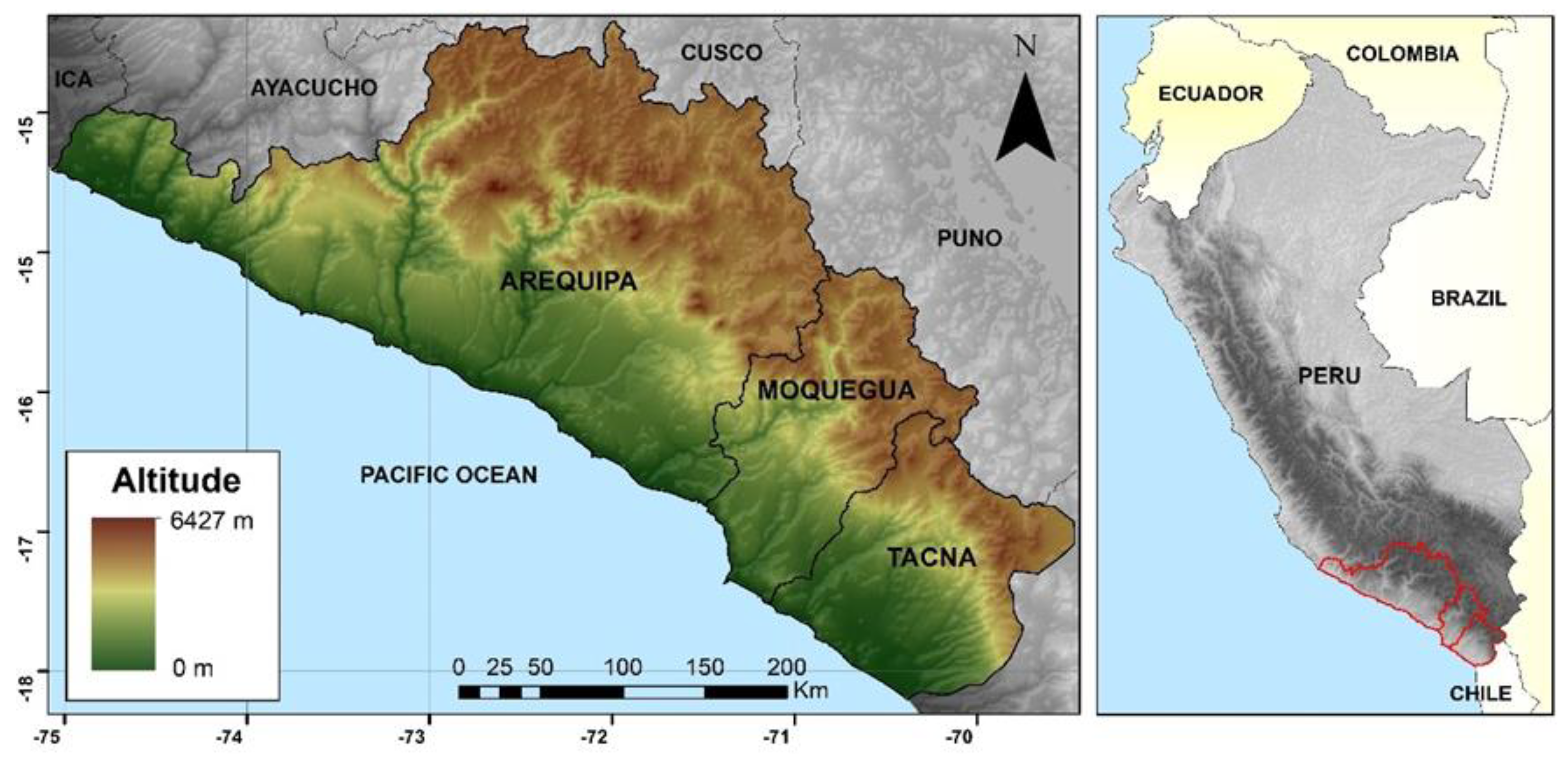
Figure 2.
Distribution of the meteorological stations in the departments of Arequipa, Moquegua, and Tacna.
Figure 2.
Distribution of the meteorological stations in the departments of Arequipa, Moquegua, and Tacna.
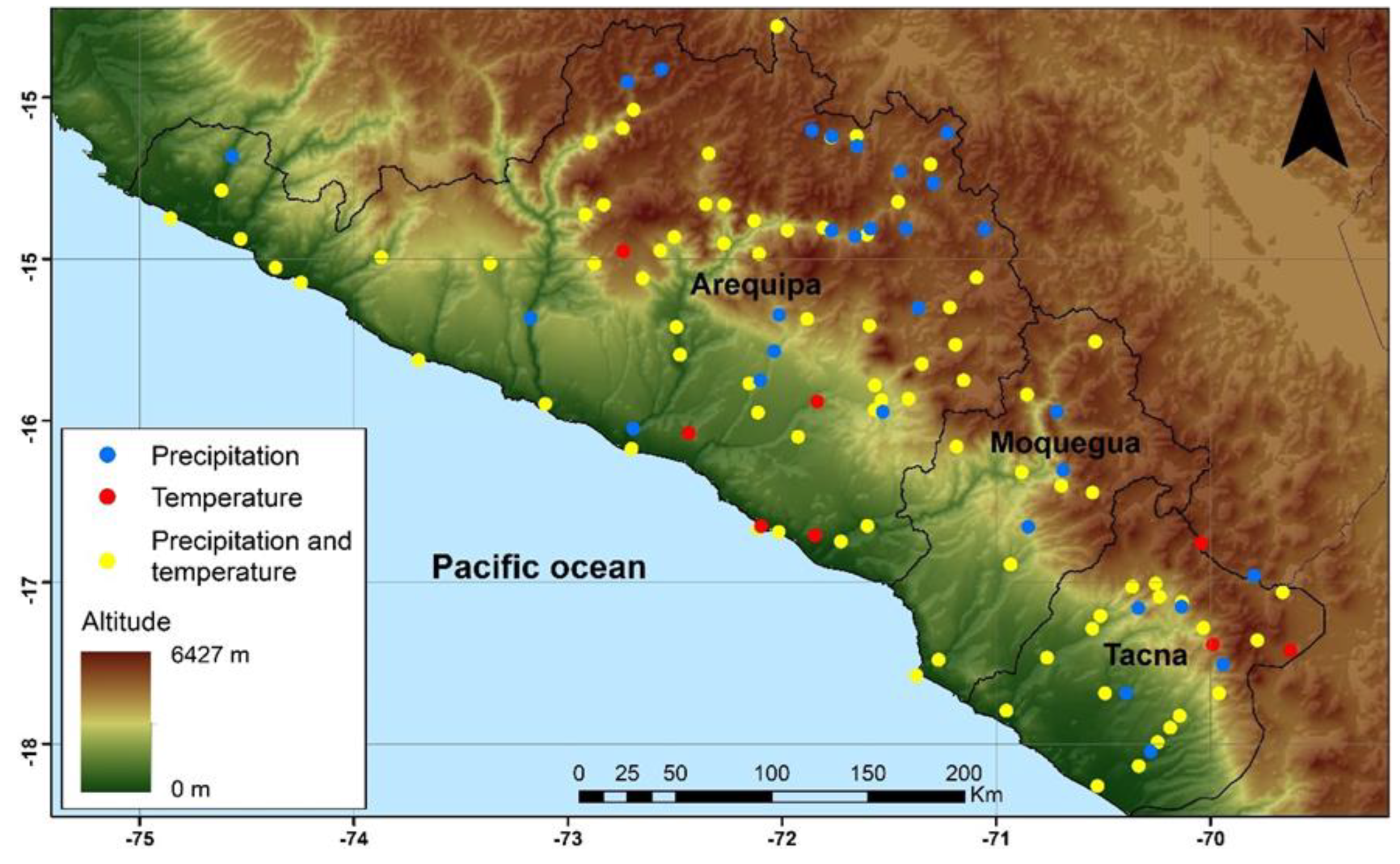
Figure 3.
(A) Monthly mean temperature variability for the stations sampled in this study; (B) Precipitation variability for the stations located in the coastal area (<1500 m.a.s.l.); and (C) Precipitation variability for stations located in the Andean area (>1500 m.a.s.l.).
Figure 3.
(A) Monthly mean temperature variability for the stations sampled in this study; (B) Precipitation variability for the stations located in the coastal area (<1500 m.a.s.l.); and (C) Precipitation variability for stations located in the Andean area (>1500 m.a.s.l.).

Figure 4.
(A). Surface for mean annual maximum temperature (°C); (B). Mean annual minimum temperature (°C), (C). Mean annual accumulated precipitation (mm) from 0 to 1500 m.a.s.l.; and, (D). Mean annual accumulated precipitation (mm) from 1500 to >4500 m.a.s.l.
Figure 4.
(A). Surface for mean annual maximum temperature (°C); (B). Mean annual minimum temperature (°C), (C). Mean annual accumulated precipitation (mm) from 0 to 1500 m.a.s.l.; and, (D). Mean annual accumulated precipitation (mm) from 1500 to >4500 m.a.s.l.
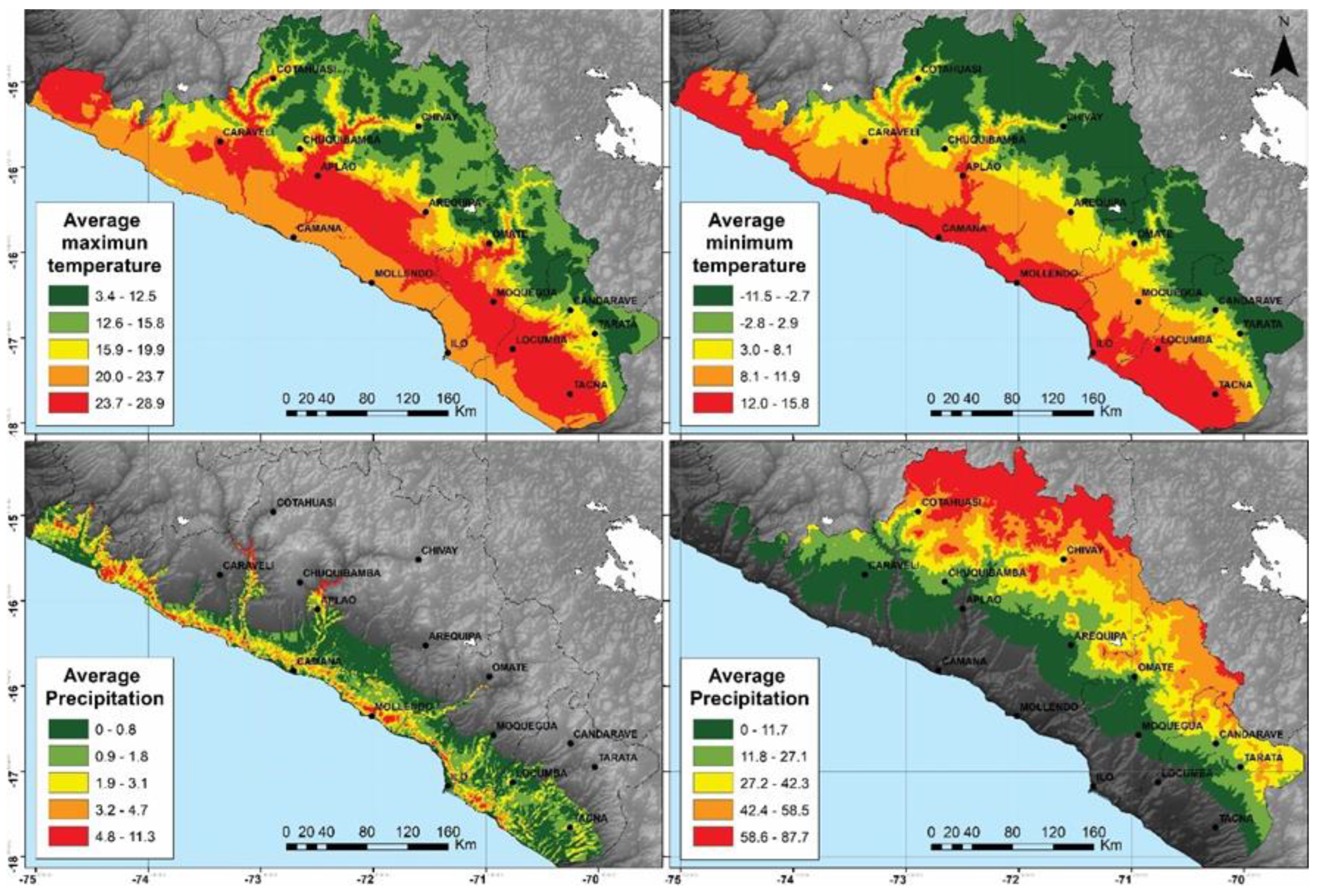
Figure 5.
Representation of the statistics produced for each of the monthly climatic surfaces made (rectangles indicate value range; squares within rectangles are the data mean; bars within rectangles indicate the standard deviation. As for precipitation, the bottom part of the bar indicate the mean). (A). Maximum Temperature (°C); (B). Minimum Temperature (°C); and (C). Precipitation (mm).
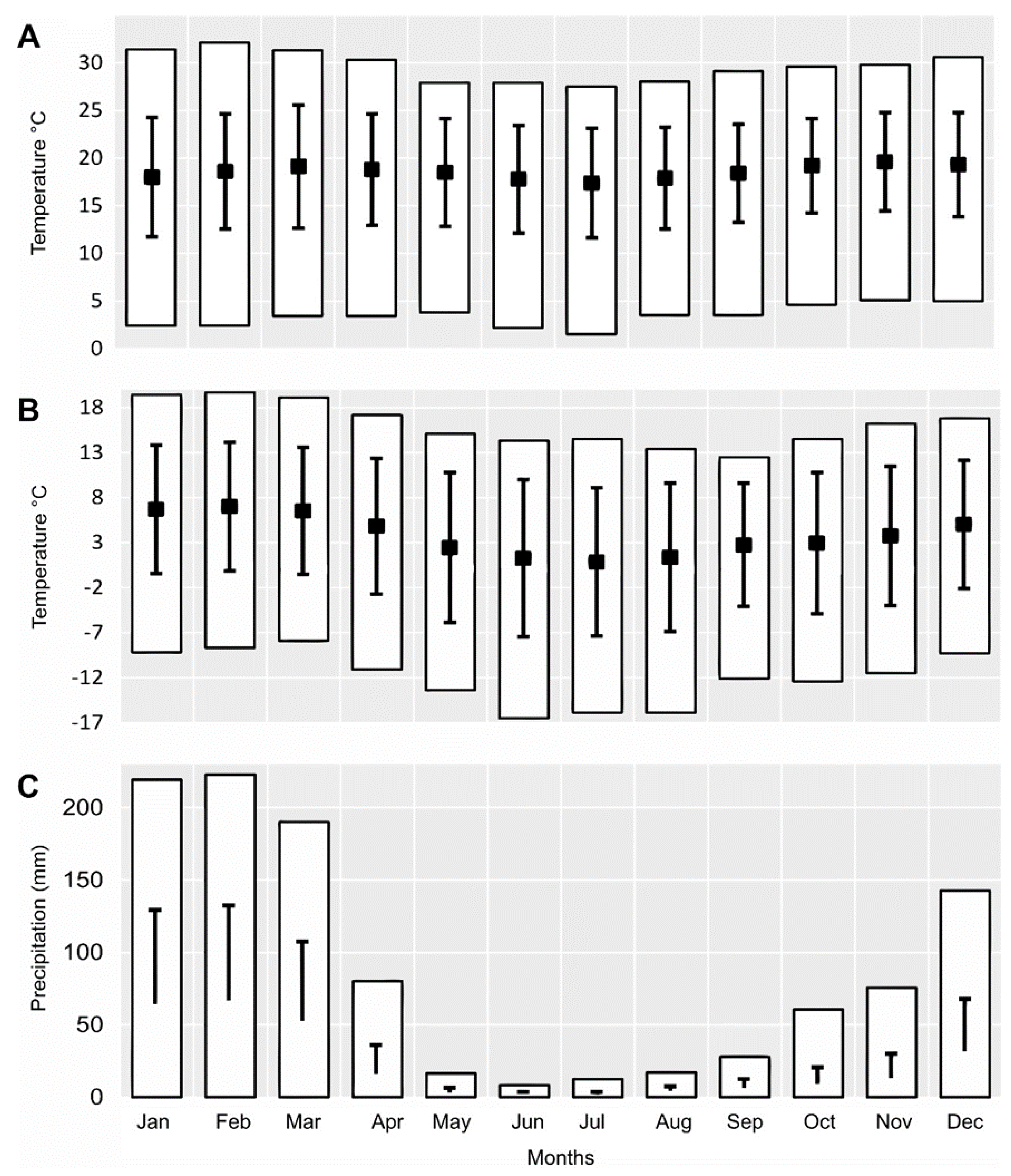
Figure 6.
Patterns of variables produced according to altitudinal gradient (0–6427 m.a.s.l., shown in red), orientation (north-east, 45°), and coast–inland distance (0–233 km). (A). Maximum Temperature; (B). Minimum Temperature; and (C). Precipitation.
Figure 6.
Patterns of variables produced according to altitudinal gradient (0–6427 m.a.s.l., shown in red), orientation (north-east, 45°), and coast–inland distance (0–233 km). (A). Maximum Temperature; (B). Minimum Temperature; and (C). Precipitation.
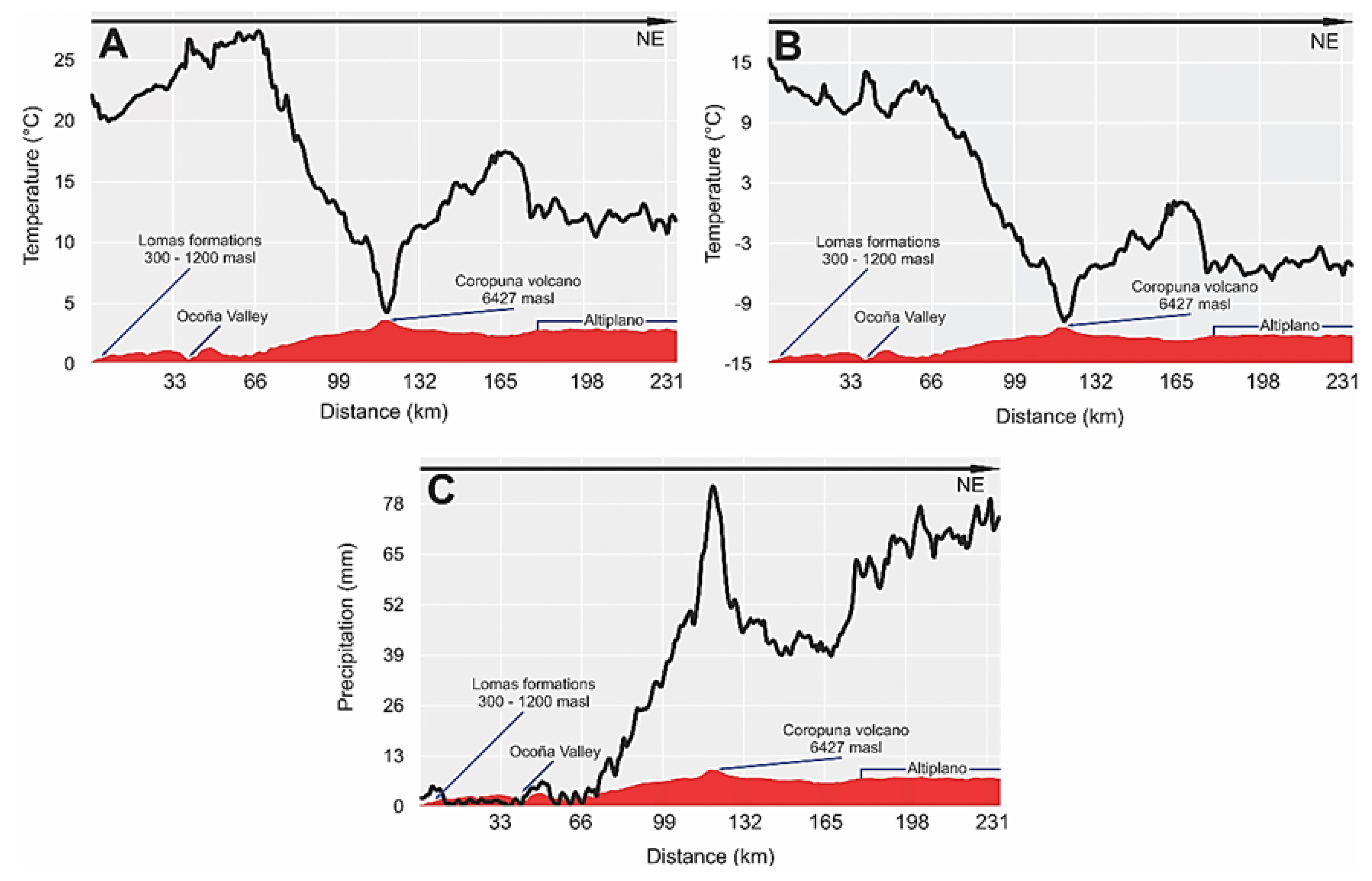
Figure 7.
Comparison of the variability of the model prepared with WorldClim 2 and CHELSA data. (A) Accumulated annual precipitation for the coastal area; (B) Accumulated annual precipitation for the Andean area; and (C) Average temperature for the whole area of study.
Figure 7.
Comparison of the variability of the model prepared with WorldClim 2 and CHELSA data. (A) Accumulated annual precipitation for the coastal area; (B) Accumulated annual precipitation for the Andean area; and (C) Average temperature for the whole area of study.
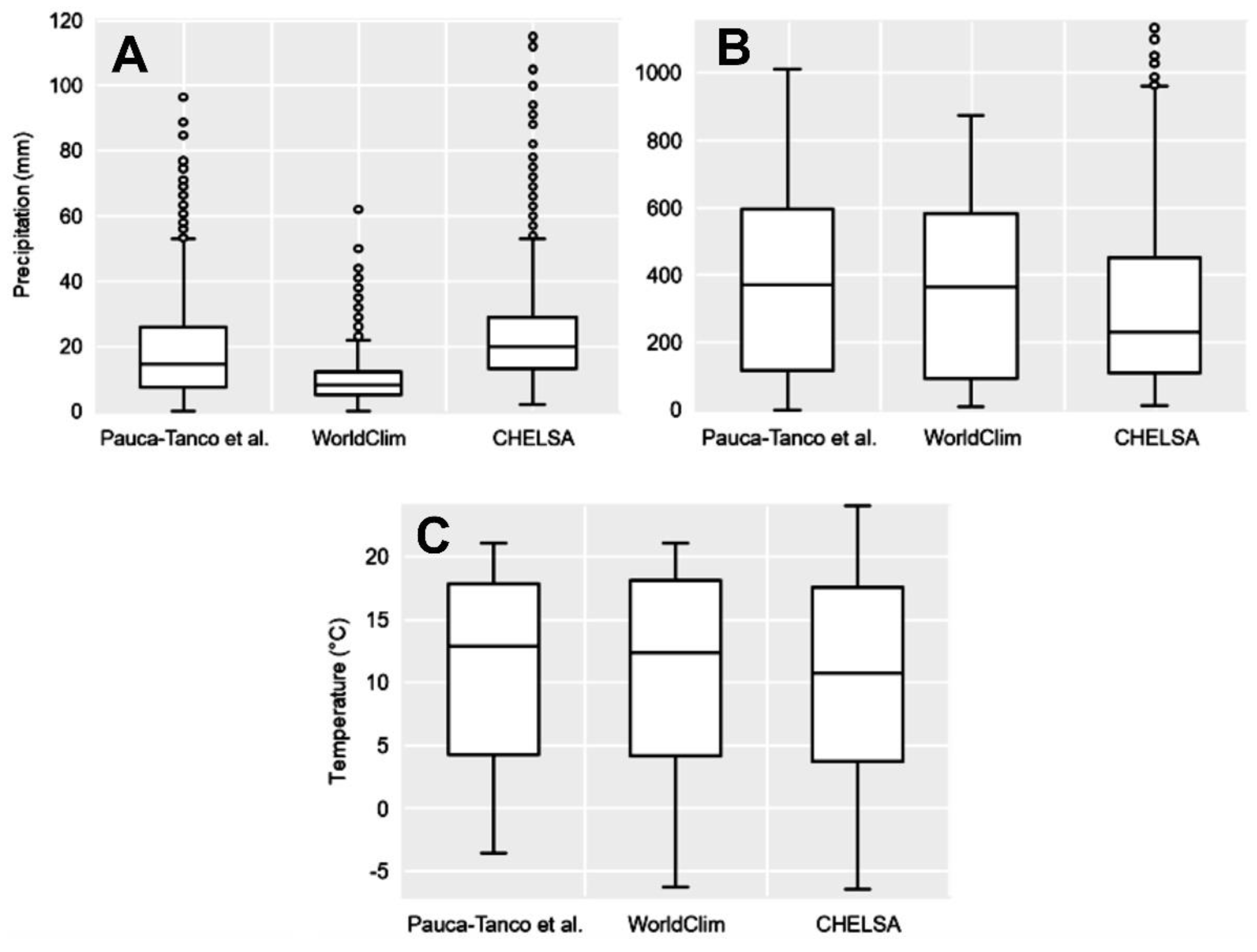

Table 1.
Statistical values obtained for maximum temperature.
| Surfaces | Jan | Feb | Mar | Apr | May | Jun | Jul | Aug | Sep | Oct | Nov | Dec |
|---|---|---|---|---|---|---|---|---|---|---|---|---|
|
Mean (SD) |
18.8 (6.2) |
18.6 (6.0) |
19.1 (6.4) |
18.8 (5.8) |
18.5 (5.6) |
17.8 (5.6) |
17.4 (5.7) |
17.9 (5.3) |
18.4 (5.1) |
19.2 (4.9) |
19.6 (5.1) |
19.3 (5.4) |
| Min V | 2.4 | 2.4 | 3.4 | 3.4 | 3.8 | 2.2 | 1.5 | 3.5 | 3.5 | 4.6 | 5.1 | 5.0 |
| Max V | 31.4 | 32.1 | 31.3 | 30.3 | 27.9 | 27.9 | 27.5 | 28.0 | 29.1 | 29.6 | 29.8 | 30.6 |
| 95% CI | 0.02 | 0.02 | 0.02 | 0.02 | 0.02 | 0.02 | 0.02 | 0.02 | 0.02 | 0.02 | 0.02 | 0.02 |
SD: Standard deviation; Min V: Minimum value; Max V: Maximum value; CI: 95% confidence interval.
Table 2.
Statistical values obtained for minimum temperature.
| Surfaces | Jan | Feb | Mar | Apr | May | Jun | Jul | Aug | Sep | Oct | Nov | Dec |
|---|---|---|---|---|---|---|---|---|---|---|---|---|
|
Mean (SD) |
7.2 (7.2) |
7.5 (7.2) |
7.0 (7.1) |
5.3 (7.6) |
2.9 (8.4) |
1.7 (8.8) |
1.3 (8.3) |
1.8 (8.3) |
3.2 (6.9) |
3.4 (7.9) |
4.2 (7.8) |
5.5 (7.2) |
| Min V | -9.2 | -8.7 | -7.9 | -11.1 | -13.4 | -16.5 | -15.9 | -15.9 | -12.1 | -12.4 | -11.5 | -9.3 |
| Max V | 19.4 | 19.7 | 19.1 | 17.2 | 15.1 | 14.3 | 14.5 | 13.4 | 12.5 | 14.5 | 16.2 | 16.8 |
| 95% CI | 0.03 | 0.03 | 0.03 | 0.03 | 0.03 | 0.03 | 0.03 | 0.03 | 0.02 | 0.03 | 0.03 | 0.03 |
DS: Standard deviation; Min V: Minimum value; Max V: Maximum value: CI: 95% confidence interval.
Table 3.
Statistical values obtained for accumulated precipitation.
| Surfaces | Jan | Feb | Mar | Apr | May | Jun | Jul | Aug | Sep | Oct | Nov | Dec |
|---|---|---|---|---|---|---|---|---|---|---|---|---|
|
Mean (SD) |
65.0 (65.4) |
67.3 (66.2) |
53.2 (55.2) |
16.3 (20.1) |
3.3 (3.4) |
2.2 (1.6) |
2.0 (1.7) |
4.3 (3.4) |
6.5 (6.2) |
9.4 (11.6) |
13.3 (17.1) |
32.0 (36.6) |
| Min V | 0 | 0 | 0 | 0 | 0 | 0 | 0 | 0 | 0 | 0 | 0 | 0 |
| Max V | 219.2 | 222.8 | 190.2 | 80.1 | 16.4 | 8.2 | 12.4 | 16.9 | 27.8 | 60.6 | 75.6 | 142.8 |
| 95% CI | 0.23 | 0.24 | 0.20 | 0.07 | 0.01 | 0.01 | 0.01 | 0.01 | 0.02 | 0.04 | 0.06 | 0.13 |
SD: Standard deviation; Min V: Minimum value; Max V: Maximum value: CI: 95% confidence interval.
Table 4.
RMSD, MAD, and R2 values for the interpolated variables.
| Months | Maximum Temperature (°C) | Minimum Temperature (°C) | Precipitation (mm) | |||
|---|---|---|---|---|---|---|
| RMSEcv | MADE | RMSEcv | MADE | RMSEcv | MAD | |
| January | 1.5 | 1.1 | 0.8 | 0.6 | 11.6 | 8.2 |
| February | 1.5 | 1.2 | 0.8 | 0.7 | 12.2 | 8.6 |
| March | 1.5 | 1.1 | 0.8 | 0.6 | 10.1 | 7.0 |
| April | 1.4 | 1.1 | 1.0 | 0.7 | 5.7 | 3.6 |
| May | 1.4 | 1.1 | 1.5 | 1.0 | 1.6 | 1.2 |
| June | 1.4 | 1.1 | 1.7 | 1.2 | 1.3 | 1.0 |
| July | 1.4 | 1.0 | 1.8 | 1.2 | 1.6 | 1.1 |
| August | 1.5 | 1.1 | 1.7 | 1.2 | 2.4 | 1.8 |
| September | 1.7 | 1.2 | 1.4 | 1.1 | 3.5 | 2.7 |
| October | 1.6 | 1.2 | 1.1 | 0.8 | 5.0 | 3.4 |
| November | 1.7 | 1.3 | 1.1 | 0.8 | 5.0 | 3.4 |
| December | 1.6 | 1.2 | 0.9 | 0.7 | 9.2 | 6.1 |
| Average | 1.5 | 1.1 | 1.2 | 0.9 | 5.8 | 4.0 |
RMSEcv: root mean square deviation of cross-validation; MAD: mean absolute deviation of error.
Table 5.
Statistical characteristics for the compared surfaces.
| Variables | A | B | C |
|---|---|---|---|
| Coastal Precipitation (mm) | n = 2000 | ||
| Mean (SD) | 18.8 (15.4) | 9.5 (7.7) | 23.2 (15.1) |
| Median (Q1, Q3) | 14.0 (8.0–26.0) | 8.0 (5.0–12.0) | 20.0 (13.0–29.0) |
| Range | 0.0–96.0 | 0.0–62.0 | 2.0–116.0 |
| P value | - | < 0.01* | < 0.01* |
| Andes Precipitation (mm) | n = 2000 | ||
| Mean (SD) | 378.1 (271.3) | 355.4 (254.8) | 302.2 (240.3) |
| Median (Q1, Q3) | 408.0 (118.0–594.0) | 363.5 (94.8–581.3) | 230.0 (109.8–451.0) |
| Range | 0.0–1011.0 | 9.0–873.0 | 14.0–1151.0 |
| P value | - | < 0.05 | < 0.01* |
| Temperature (°C) | n = 4000 | ||
| Mean (DS) | 11.43 (6.54) | 11.25 (6.75) | 10.84 (7.22) |
| Median (Q1, Q3) | 12.90 (4.3–17.8) | 12.35 (4.2–18.01) | 10.70 (3.7–17.6) |
| Range | -3.60–21.00 | -6.30–21.10 | -6.40–24.00 |
| P value | - | 0.498 | < 0.01* |
A = This study; B = WorldClim 2 and C = CHELSA. * Shows highly-significant differences.
Disclaimer/Publisher’s Note: The statements, opinions and data contained in all publications are solely those of the individual author(s) and contributor(s) and not of MDPI and/or the editor(s). MDPI and/or the editor(s) disclaim responsibility for any injury to people or property resulting from any ideas, methods, instructions or products referred to in the content. |
© 2023 by the authors. Licensee MDPI, Basel, Switzerland. This article is an open access article distributed under the terms and conditions of the Creative Commons Attribution (CC BY) license (http://creativecommons.org/licenses/by/4.0/).
Copyright: This open access article is published under a Creative Commons CC BY 4.0 license, which permit the free download, distribution, and reuse, provided that the author and preprint are cited in any reuse.


