
Submitted:
17 February 2023
Posted:
20 February 2023
You are already at the latest version
Abstract
Healthcare professionals and resource planners can use healthcare delivery process mining to ensure the optimal utilisation of scarce healthcare resources when developing policies. Within hospitals, patients' Length of Stay (LOS) and volume of admitted patients, in terms of number and characteristics (age, gender, and social deter-minants), are significant factors determining daily resource requirements. In this study, we used Coxian phase-type Distribution (C-PHD) based Phase-Type Survival (PTS) trees for analysing how covariates such as admission date, gender, age, district, and admissions source influence the admission rate and LOS distribution. PTS trees. This study used a two-year data set (2011-2012) of patients admitted to the Emergency Department at Mater Dei Hospital to generate models and an independent one-year data set (2013) of patients admitted to the Emergency Department at Mater Dei Hospital to evaluate. The PTS tree effectively clusters patients based on their LOS, considering the prognostic significance of different covariates related to patients' characteristics. Charac-terising these covariates provided meaningful results about LOS. Similarly, the PTS tree was used to effectively cluster patients based on the admission rate, considering the prognostic significance of these covariates.
Keywords:
Length of stay estimation
; Admission rate characterization
; Resource requirement forecasting
; Patientcare modelling
; Hospital capacity planning
; Phase type survival trees
; Machine Learning
; Health ML Extended Health Intelligence
1. Introduction
By forecasting daily resource requirements for admissions, healthcare planners can develop a plan to ensure the efficient and effective quality of service at a minimal cost [8] to ensure the ideal use of resources [11]. Complex strategies are often required to solve problems of admission scheduling and resource requirements to efficiently and effectively manage the healthcare system. Healthcare planners frequently experience dilemmas of ensuring equitable allocation of hospital resources when faced with long waiting lists and overcrowded emergency departments having patients waiting for admission. Thus, by finding an efficient solution to this problem, it is possible to help healthcare resource managers, hospital staff, and policymakers make the hospital more efficient. The aim of this project included developing a mathematical model, which may be used to model LOS and admissions patterns through PTS trees [8,10,11,12,28,29,30]. Developing this model will help healthcare professionals create policies that ensure the optimal allocation of the limited resources available. This model would then predict patients' LOS and the number of admissions for independent data.
1.1. Background and Previous Research
There has been tremendous interest in estimating the hospital length of stay from a long time [31,32] and the factors affecting it [17,18] and recent studies [33,34,35,36,37,38,39,40,41,42,43,44,45,46,47,48,49,50,51,52,53,54,55,56,57,58,59,60,61,62,63,64,65,66,67,68,69,70,71,72,73,74,75,76,77,78,79,80,81,82,83,84,85]. There are some recent reviews of machine learning and statistical methods for the hospital length of stay estimation. [43,48,51,62,68]. Keegan [18] argued in favour of evidence showing that bed occupancy rate is a reliable key performance indicator for hospitals' capability to provide good quality care to patients. Cooke et al. [3] suggested that if a border is set and the bed occupancy rate is below it, then the waiting times in the Emergency Department will be reduced exceptionally. Jones [17] discussed several factors which affect hospital occupancy demand, including temperature (admissions may increase or decrease the possibility of certain conditions), injuries and infections (these do not happen during certain periods and have no significant patterns), clinical practice changes, weather and environmental factors such as viruses and the rising need of end-of-life care.
Many models have been developed in the past, some of which include queuing models (Worthington D. J. [24], Gorunescu et al. [9]). In contrast, others use computer simulation or population ratio-based models (Kuzdrall et al. [19]). Fackrell [4] suggested that a realistic approach to modelling a care system uses compartmental models mainly implemented using phase-type Distribution (PHD). However, these models are unsuitable for admission scheduling and capacity planning since they mostly model patient flow within the hospital and do not consider re-admissions or community care. Garg et al. [20] proposed an alternative model developed using Markov chain modelling where the resource necessities could be forecasted using patient pathways in the future. In this study, Markov Chains were used to construct a policy that satisfies any future resource availability for the care system. However, this study is limited since it assumes a fixed number of daily admissions, which is unrealistic and cannot be used for many practical situations. In a further study by Garg et al. [11], a model was introduced where scheduling admissions, allocating resources and forecasting requirements could be achieved. This model improves the previously mentioned model [20] since it may be used for fixed and variable daily admissions. The model presented in the study [11] considers two time-dependent covariates: the current calendar year and the patient's current age. The covariates for each patient are updated daily to have a more realistic model. This model is mainly based on predictable values and can therefore forecast the number of expected patients in each phase and the daily cost of care. The authors of a further study (Garg et al. [8]) propose using covariates, such as age, gender, time of admission and diagnosis, to carry out better hospital capacity planning since these characteristics affect a patient's LOS. In this study, a PTS tree is used for smaller patient groups with respect to the LOS distribution using the characteristics as a base. In this paper, Garg et al. [8] propose an adaptable and flexible approach to intelligent healthcare planning and patient organisation, considering patient heterogeneity, essential variability and system complexity.
1.1.1. The seasonal Effect on Patient Admissions
Moreover, patients' admission could also be affected by several seasonal effects. Fullerton & Crawford [6] states that patient admission increases substantially during winter, mainly in general medicine and orthopaedics. This study also found fewer admissions during Christmas than the rest of the year. Green, Fullerton and Crawford ([6], [13]) agree that fewer procedures are booked for the weekend, and no elective patients are admitted to keeping bed space for weekend demand. Fullerton & Crawford [6] believe that the seasonal effect is predictable. Therefore, chaos within hospitals could be avoided if healthcare planners had to plot the admission rates better and better utilise the resources of primary care institutions.
1.1.2. Models Used to Estimate the Patient's Length of Stay
Estimating the LOS of patients helps resource planners analyse and estimate the hospital's bed occupancy and thus forecast the required resources. The two most popular methods that provided almost accurate approximations in previous studies when estimating patient LOS include the Gaussian Mixture Model and the C-PHD. Using phase-type distributions in various stochastic models allows algorithmically tractable solutions to be found. General PHDs are said to be over-parametrised (Fackrell [4], Marshall A, McClean S. [21]). C-PHD are a subclass of general PHDs which requires less complex parameter estimation (Fackrell [4]). The literature provides different methods to approximate the parameters [4]. These methods included:
Maximum likelihood estimation (Asmussen et al. [2], Olsson [23], Faddy & McClean [7], Faddy [5] and Hampel [14]).
Moment matching (Johnson [16])
Least squares
Splitting the main part and the tail part of the distribution (defined on positive numbers with a PHD) and approximating them separately (Horvath and Telek [1]).
2. Materials and Methods
In this study, the patient flow within the hospital system is to be modelled. In several studies ([20], Garg et al. [11]), patient flow is categorised through the rate of transition of a patient between states. It is assumed that there are n hospital phases (acute, treatment, rehabilitation, long stay) and m community phases (dependent, convalescent, recovered). Patients move sequentially from one hospital phase to the next and similarly from one community phase to the next. A patient may be re-admitted into the first hospital phase from any community phase and may be discharged from any hospital phase to the first phase or die at any point in the process. Furthermore, the set-up consists of n hospital phases and one absorbing state within this study. This may be represented as a discrete-time Markov chain having n+1 states. In this model, patients are admitted in the first state. They could leave the system at any other state (through death or by being discharged). Figure 1 describes the possible patient flow through the system, where: HPi represents being in hospital phase i, λi represents the transmission rate between HPi to HPi+1, and μi represents the transmission rate between HPi and the absorbing state, death or community phase. Therefore, as mentioned above, this study models patient flow within the healthcare system using C-PHD and PTS. These two distributions are further described below.
2.1. Coxian Phase-Type Distribution
C-PHD is a special type of PHD. It is defined as an n-state continuous Markov process with a single absorbing state which may be reached from any phase instead of only being reached from state n. Admission into the system may only be from the first state, allowing sequential movement through the states [10]. This study uses C-PHDs to model patient flow, as shown in Figure 1. The initial state distribution, p, is defined as [10]:
the vector q denotes the absorption probabilities and is defined as:
and the transition matrix Q is defined as [10]:
From these definitions, the log-likelihood function is obtained [10], where N is the total number of patients in the healthcare system and ti is the LOS of patient i.
Within our study, the above function is used to create PTS trees.
2.2. Phase-Type Survival Tree
Survival trees are a regression tool used to perform survival analysis [10]. It is an effective and efficient method of collecting survival data and understanding its connection with covariates, results from treatments and LOS data. A PHD distinctly models each node in a PTS tree. PTS trees have been used to model many applications in medical research, including forecasting bed requirements. In Garg et al. [10] study, PTS trees are implemented to cluster patients' lengths of stay.
PTS trees are created by repetitively partitioning the data into subsections depending on covariates through splitting and selection conditions aiming to maximise within-node similarity or between-node splits [12]. Splitting maximises node similarity based on improving log-likelihood functions [12].
The weighted-Average information criterion (WIC) is a weighted average of Akaike's information criteria (AIC) and the Bayesian information criteria (BIC) with a small sample size correction [8]. As the splitting criteria based on the WIC combines the strengths of both the AIC and the BIC, it works well with small and large sample sizes and also in the case when the sample size is not known [25]. The following formula is used to calculate the WIC [8]:
Since C-PHD is being used, each node is modelled separately. If a covariate X has k values and the node splits into k partitions, then the WIC for the split can be calculated using equation 5. After splitting the node by the covariate, the WIC gain can be calculated in equation 6, where WIC0 is the WIC before splitting [8].
(6[M1] )
This study uses split and selection criteria to maximise node homogeneity as recommended as the most suitable criterion by [30]. The node that minimises the WIC is selected to recursively divide the node into child nodes by starting at the root node. If a node with a negative gain occurs, then the node is set as a terminal node, and no more splitting occurs. This is the stopping criteria.
3. Implementation
The EMphy package is used in which all algorithms and models are implemented in MATLAB using a PHD fitting program [22]. This package, developed by Asmussen et al. [2], uses the expectation minimisation algorithm to calculate the maximum likelihood parameter estimations.
3.1. The Dataset and Some Data Analysis
The results obtained from this study are based on datasets provided by Mater Dei Hospital, Malta and Free Metro, Online. Mater Dei Hospital provided data for patients discharged during 2011 and 2012. The patient data provided by Mater Dei was confidential and did not include any personal information. The covariates present in the data provided by Mater Dei Hospital included gender, age, locality of residence, source admission and discharge location, admissions and discharge wards and admission and discharge dates. Admission type is a crucial distribution of admission data represented in Table 1. We divided admission into three groups and included fields as No. of admissions, total Days spent during LOS and Average days spent during LOS.
3.1.1. Admissions Data
Between 2011 and 2012, 66601 and 68903 patients were admitted to Mater Dei Hospital. Table 2 depicts the number of admissions occurring each day of the week for each month throughout both years. From Table 2, the maximum number of admissions (2423 patients) occurred on Mondays during January, whilst the least number of admissions (849 patients) occurred on Sundays in August. From Table 2 and Figure 2, it could also be seen that the maximum number of admissions occurred during October when 12208 patients were admitted to the hospital. The minimum number of admissions occurred in December when 10001 patients were admitted to the hospital. From this data, it was observed that January, October and November are the months most patients were admitted to the hospital. Additionally, it may be seen from Figure 3 that the number of admissions is reduced substantially during the weekend. Figure 4 confirms that fewer elective and day cases are admitted during the weekend, mainly Saturday and Sunday, compared to the rest of the week. It may then be seen that the number of admissions on a Monday is much higher than the rest of the week in all three types of admissions. This agrees with previously mentioned studies by Fullerton and Crawford [6] and Green [13]. These authors agree that fewer procedures are booked during weekends to keep bed space for weekend demand.
3.1.2. Covariants
The covariates Gender, Age, District and SourceAdm were grouped into three groups, four groups, seven districts and five groups, respectively. The Gender covariate groups are; Male, Female and Unclassified and the Age covariate groups are; Age 0 (NewBorn), Ages 1 to 30 (Under30), Ages 31 to 70 (Under70) and Ages 70 to 105 (Over71). Admissions of patients over 70 have an average LOS of approximately 5.91, longer than younger patients (excluding newborns) average LOS 6.8.
The Locality of Residence covariate groups may be seen in table 3. These groupings were carried out to have better performance when running. Residents of Gozo and Comino had the minimum average LOS of 2.92 days, while the North of Malta had the longest average of 3.89 days. The SourceAdm covariate (the source of admission) groups are; Private Residence Home/ Usual Residence, Home for the Elderly (including St Vincent de Paule Residence and Zammit Clapp Hospital), Other (including Gozo Hospital, Labour Ward, Nursery, Public Hospitals (Government Institutes including Boffa Hospital & Mount Carmel Hospital) and Private and Foreign Hospitals), Police Custody and Unknown. Table 3 gives the number of admissions, total, and average LOS for each covariate group.
3.2. Phase-Type Survival Trees
The following PTS trees were generated using the WIC-based spitting criteria for the emergency data provided by Mater Dei Hospital. This approach was used to analyse the length of stay and admission patterns.
3.2.1. Length of Stay Analysis
Table 4, Table 5, Table 6, Table 7, Table 8, Table 9, Table 10, Table 11, Table 12, Table 13, Table 14, Table 15, Table 16, Table 17, Table 18, Table 19, Table 20, Table 21, Table 22, Table 23, Table 24, Table 25 and Table 26 represents the steps used to generate the LOS PTS tree shown in Figure 5, representing the WIC-based splitting criteria from the LOS data against the covariates related to the patient's characteristics.
First, we fit the complete data (represented as a root node (1) in Figure 5 and Table 4) to Coxian Phase Type Distribution (C-PTD) and calculate its WIC. Then, for each covariate, we split the LOS data and fit each group individually to C-PTD, total the C-PTD and compare it WIC of the root node (i.e., before the split) to calculate the gain in C-PTD. We select the covariate providing the maximum positive gain in C-PTD to split the data. Table 4 shows that covariate “Age“ offers the maximum positive gain in C-PTD. Therefore, we select this split to grow the tree. New nodes are shown in Figure 5 as 2 (newborn), 7 (under 30), 10 (under 70) and 20 (over 70).
Step 2: we split the LOS data for each remaining covariate (Gender, District and SourceAd), fit each group individually to C-PTD and total the C-PTD and compare the WIC of the node before the split to calculate the gain in C-PTD. We select the covariate providing the maximum positive gain in C-PTD to split the data. Here, in Table 5, Table 6, Table 7 and Table 8, for nodes 2 (newborn) and 7 (under 30), covariate “Gender“, while for nodes 10 (under 70) and 20 (over 70) covariate “District” offer the maximum positive gain in C-PTD. Therefore, we select this split to grow the tree, and new nodes are shown in Figure 5 as 3, 6, 8, 9, 11, 12, 13, 14, 15, 16, 19, 21, 24, 27, 28, 29, 30, and 33.
Step 3: Nodes 3, 6, 8, 9, 11, 12, 13, 14, 15, 16, 19, 21, 24, 27, 28, 29, 30, and 33 are splitted by remaining covariates, and fit each group individually to C-PTD and total the C-PTD and compare it WIC of the root node (i.e., before the split) to calculate the gain in C-PTD. We select the covariate providing the maximum positive gain in C-PTD to split the data. Here, in Table 5, Table 6, Table 7 and Table 8 for node 2 (newborn) and 7 (under 30), we can see covariate “Gender“ offers the maximum positive gain in C-PTD, while for node 10 (under 70) and 20 (over 70) it is covariate District. Therefore, we select this split to grow the tree and new nodes are shown in Figure 5 as 3, 6, 8, 9, 11, 12, 13, 14, 15, 16, 19, 21, 24, 27, 28, 29, 30, and 33.
Table 9, Table 10, Table 11, Table 12, Table 13, Table 14, Table 15, Table 16, Table 17, Table 18, Table 19, Table 20, Table 21, Table 22, Table 23, Table 24, Table 25 and Table 26 show that only nodes 3 and 16 provided significant WIC improvement with a split by sourceAd, and nodes 21, 24 and 30 provided significant WIC improvement with a split by gender. All remaining nodes did not provide any significant WIC improvement by any split and therefore considered terminal nodes. In Figure 5, there are 23 terminal nodes representing the data's significant clusters. The survival plots for all the terminal nodes are shown in Figure 6, which outlines the model's goodness of fit. The total gain in WIC obtained is 5782.13, where the WIC of the root node is 355134.92, and the terminal nodes' WIC sum up to 349352.79. It is possible to identify the relationship between the patient's characteristics and their LOS by analysing Table 4, Table 5, Table 6, Table 7, Table 8, Table 9, Table 10, Table 11, Table 12, Table 13, Table 14, Table 15, Table 16, Table 17, Table 18, Table 19, Table 20, Table 21, Table 22, Table 23, Table 24, Table 25 and Table 26 and Figure 5. From the table, the most significant split is by the covariate age, with a WIC gain of 6511.88. The mean LOS value may significantly differ between the age groups for each split. Figure 5 shows that the most significant split for newborns (node 2) and patients under 30 (node 7) occurred for the gender covariate. In contrast, the most significant split for patients under 70 (node 10) and patients over 71 further occurred for the district covariate. Figure 6 plots the survival function related to Personal Characteristics for each terminal node for the Length of Stay analysis to show the goodness of fit.
3.2.2. Admissions Analysis:
Table 27, Table 28, Table 29, Table 30, Table 31, Table 32, Table 33, Table 34, Table 35, Table 36, Table 37, Table 38, Table 39, Table 40, Table 41, Table 42, Table 43, Table 44, Table 45, Table 46, Table 47, Table 48 and Table 49 represent the steps used to generate the admissions PTS tree shown in Figure 7, representing the WIC-based splitting criteria from the admissions data against the covariates related to the patient's characteristics. Similar to the length of stay analysis above, here also, first, we fit the complete data (represented as a root node (1) in Figure 7 and Table 27) to Coxian Phase Type Distribution (C-PTD) and calculate its WIC. Then, for each covariate, we split the admissions data and fit each group individually to C-PTD, total the C-PTD and compare it WIC of the root node (i.e., before the split) to calculate the gain in C-PTD. We select the covariate providing the maximum positive gain in C-PTD to split the data. Table 27 shows that covariate “Source of admissions (sourceAdm)“ offers the maximum positive gain in C-PTD. Therefore, we select this split to grow the tree. New nodes are shown in Figure 7 as 2 (Home/Private Residence), 3 (Home for the elderly), 4 (other), 5 (Police Custody) and 6 (Unknown).
Step 2: we split the admissions data for each remaining covariate (Gender, Age and District), fit each group individually to C-PTD and total the C-PTD and compare the WIC of the node before the split to calculate the gain in C-PTD. We select the covariate providing the maximum positive gain in C-PTD to split the data. Here, in Table 28, Table 29, Table 30, Table 31 and Table 32 for nodes 2 (Home/Private Residence), 4 (Other admission sources) and 5 (Police Custody) covariate “District“ and nodes 3 (Home for the Elderly) and 6 (unknown admission source) covariate “Age” offer the maximum positive gain in C-PTD. Therefore, we select this split to grow the tree, and new nodes are shown in Figure 7 as 7, 12, 17, 22, 27, 32, 37, 42, 43, 49, 52, 57, 62, 67, 70, 75, 80, 81, 84, 87, 90, 92, 93, 94, and 95.
Table 33, Table 34, Table 35, Table 36, Table 37, Table 38, Table 39, Table 40, Table 41, Table 42, Table 43, Table 44, Table 45, Table 46, Table 47, Table 48, Table 49, Table 50, Table 51, Table 52, Table 53, Table 54, Table 55, Table 56 and Table 57 show that only nodes 7, 12, 17, 22, 27, 32, 37, 52, 57, 62, 67, 70, 75, 81, 84, 87 and 90 provided significant WIC improvement with a split by Age, and nodes 49, 67 and 35 provided significant WIC improvement with a split by gender and only node 43 provided significant WIC improvement with a split by District. All remaining nodes did not provide any significant WIC improvement by any split and therefore considered terminal nodes. Figure 7 shows a graphical representation of the WIC-based splitting criteria from the admissions data against the covariates, directly affecting patients' characteristics. The survival tree consists of 70 terminal nodes representing the data's significant clusters. Table 27, Table 28, Table 29, Table 30, Table 31, Table 32, Table 33, Table 34, Table 35, Table 36, Table 37, Table 38, Table 39, Table 40, Table 41, Table 42, Table 43, Table 44, Table 45, Table 46, Table 47, Table 48, Table 49, Table 50, Table 51, Table 52, Table 53, Table 54, Table 55, Table 56 and Table 57 show the results used to generate the survival tree.
Similarly to the previously generated survival tree, the average WIC is taken for the covariates Age, Gender, District and sources of Admissions. The average WIC is calculated because the root node takes the data for the whole period (721 days), while each covariate takes the whole period per subgroup. For example, considering age in each subgroup (newborn, under 30, under 70 and over 71) calculates the WIC over the same 721 days. Therefore the age would have four times the data of the root node. Therefore, for covariate Age, the average WIC is calculated by dividing the WIC per subgroup by 4. Similarly, the covariates Gender, District and Source Admissions were divided by 2, 7 and 5, respectively. This was repeated as the tree was further split. The total gain in WIC obtained is 2378.89, where the WIC of the root node is 2561.45, and the terminal nodes' WIC sum up to 182.56. It is possible to analyse the relationship between the patient's characteristics and admissions using the results from Table 27, Table 28, Table 29, Table 30, Table 31, Table 32, Table 33, Table 34, Table 35, Table 36, Table 37, Table 38, Table 39, Table 40, Table 41, Table 42, Table 43, Table 44, Table 45, Table 46, Table 47, Table 48, Table 49, Table 50, Table 51, Table 52, Table 53, Table 54, Table 55, Table 56 and Table 57 and Figure 7. It may be seen that the most significant split occurs for the source of admissions covariate with a WIC gain of 4348.46. The next level shows that the most significant splits occurred for the district covariate for three groups (private residence, other and police custody) and the age covariate for two groups (elderly homes and unknown).
4. Result & Evaluation
A model's Goodness-of-fit (GOF) describes how well-observed data fits into a model. By deriving the GOF, it is possible to evaluate the effect covariates have on the model fit. One of the most popular methods used as a GOF statistic is log-likelihood. Usually, the log-likelihood function is calculated by approximating the chi-square distributions and determining significance levels. The smaller result from the log-likelihood function provides a better-fit model. If the result is 0, then the model is a perfect fit [15]. A model's GOF may be assessed using GOF statistics or GOF indices. However, GOF statistics provide problems due to the small expected probabilities of obtaining accurate p-values. Due to this, most researchers prefer to make use of GOF indices. The two popular GOF indices include AIC and BIC.
Authors Wu and Sepulveda [25] showed that the WIC provides strength and stability over the models tested (including AIC and BIC etc.). The results also showed that for a small sample size, WIC performs as well as AIC. On the other hand, for a large sample size, WIC results are as well as BIC results; however, WIC exceeds the results from other criteria. This highlights the strength of WIC.
Therefore, from the literature reviewed above, it could be concluded that using WIC and log-likelihood to generate the models provides strong and stable results and, thus, models.
4.1. Predictions:
This section tests the accuracy of the predicted mean LOS values for the LOS analysis models generated. Figure 5 and Figure 7 and their respective tables 11 and 12 (In the appendix) display the significant clusters based on patients' LOS and their relationship with temperature and patient characteristics, respectively. A total of 23 clusters are generated for the relationship with patient characteristics. The mean number of admissions for all the data with the same clusters is calculated from the 2013 data. From the respective PTS tree generation tables in Appendix A, the mean LOS of each terminal node corresponding to the group is taken and recorded. The diff between these values gives the Forecasting Error result.
4.1.1. Personal Characteristics Model
Table 58 tests the accuracy between the actual and predicted data for patient characteristics, i.e. using the covariates gender, age, district and source of admissions. The table shows that the highest percentage error of over 50% is the cluster for female patients from Gozo or Comino over the age of 71 (percentage error = 53.5%). This is followed by male patients from Gozo or Comino over the age of 71 who also have quite a high percentage error of 33.36%. In another cluster, patients under 70 from an unspecified locality have a percentage error above 20% (percentage error = 21.56%). It may also be seen that apart from these three groups, all other clusters have a low percentage error of below 16%.
4.2. Admissions Analysis
This section tests the accuracy of the predicted mean number of admissions for the admissions analysis models generated. Figure 7 and respective tables 14 (In the appendix) display the significant clusters based on the number of patients admitted and their relationship with temperature and patient characteristics, respectively. Seventy clusters are generated for the relationship with the patient characteristics. All clusters are tested for the admissions analysis against patient characteristics 10 clusters are chosen to be tested for accuracy.
The mean number of admissions is calculated by counting the number of admissions and the number of records with the same clusters as those taken to be tested and dividing the number of admissions by the number of records. From the respective PTS tree generation tables in Appendix A, the respective terminal nodes are found, and the mean number of admissions of the cluster is recorded. The difference between these values gives the Forecasting Error result.
4.2.1. Personal Characteristics Model
Table 59 tests the accuracy between the actual and predicted data for patient characteristics using the covariates gender, age, district and source of admissions. Randomly ten records were selected from the 70 significant clusters, two from each level 2 subgroup in Figure 7. It may be seen (Table 59) that the highest percentage error is for the group of patients under 30 admitted from their private homes and residing in the Northern Harbour area; the percentage error value is 44.74%. The group of patients under 70 admitted from an elderly home and residing in the North had the second highest percentage error of 27.78%. Three groups had a percentage error of 0%, while three other groups had a low percentage error of under 10%. Two randomly selected clusters had no patients admitted for 2013, and thus these groups could not be tested for accuracy.
More ever, our models predict the mean and actual LOS and the number of admissions while comparing results to those of independent data. The independent data is for patients admitted in 2013 as emergency cases, provided by Mater Dei Hospital. It is important to note that this data for 2013 was not used to create the model specified above.
Table 60 calculates the Mean Square Error (MSE), Root Mean Square Error (RMSE), Mean Absolute Deviation (MAD) and the bias for all the models. MSE takes the average squared error values, the difference between the actual and predicted values. The RMSE is the square root of the mean square error, representing the standard deviation of differences between the actual and predicted value. This error test does not show whether there was an increase or decrease. MAD calculates the average absolute value of the forecasted error; it can show which forecasts deviate most. The bias calculated the forecast error average.
The error results for all the tests are close to 0, having an average forecast error of - -0.69 for the personal characteristics model. The average forecast error obtained for the patient characteristics model was -0.82, respectively.
From these results, it could be concluded that the models created can help healthcare professionals to strategically plan future resources on accurate forecasts of demands predicted by patients' characteristics. More accurate results could be obtained by splitting the covariate groups differently or considering factors like the type of emergency diagnosis. Types of cases such as surgical or chest pain may cause a patient to be admitted to the hospital, thus making patients' LOS longer than those with minor injuries such as fractures or sprains. Analysing these factors can provide more accurate results on a patient's LOS and the number of beds and resources available.
5. Conclusions
This study used a C-PHD approach on a 2-year data set (2011/2012) provided by Mater Dei Hospital and Free Metro to generate PTS trees for admissions and LOS on patient characteristics groupings for emergent patients. The PTS trees reveal the factors which significantly affect the admission rate and LOS. The average admission rate and LOS were predicted using the models and compared to the actual average admission rate and LOS for 2013 (an independent data set). The difference between the predicted and actual results was evaluated using accuracy measures. These measurement results showed that the most accurate admission model created was related to patient characteristics, while the LOS models created both showed promising results.
Further improvement to the LOS results obtained in the predictions may be achieved by extending the model to use covariates such as diagnosis, type of admission (emergency/elective), and type of procedure (e.g. BUPA classification of complex major, major+, major, intermediate and minor). Admissions results may be improved by extending the model to use day or month of admissions to accommodate daily and monthly patterns. It is also possible that admission results will be improved by considering seasonal and weekend effects. These recommendations would be carried out by running the EMpht program and reconstructing a tree using the additional covariates. Once a model that provides accurate results is created, healthcare professionals can use the model for more accurate forecasting of demand and forward planning.
Author Contributions
Conceptualisation, L.G., N.A., S.M. and N.C.; methodology, L.G., N.A., R.C. and S.M.; software, L.G., N.A. and S.M.; validation, L.G., N.A., R.C., S.M. and S.B.; formal analysis, L.G. and S.M.; investigation, L.G., N.A., S.M. and S.B.; resources, L.G., S.B. and N.C.; data curation, L.G., N.A., S.B. and N.C.; writing—original draft preparation, L.G., N.A., R.C. and B.P.; writing—review and editing, L.G., N.A., B.P. and S.B.; visualisation, L.G., N.A. and S.M.; supervision, L.G. and S.M.; project administration, L.G., S.B. and N.C.; funding acquisition, L.G., S.B. and N.C. All authors have read and agreed to the published version of the manuscript.".
Data Availability Statement
The authors will make the data used in this research available on request.
Acknowledgments
We acknowledge the Belfast City Hospital for providing data for this study.
Conflicts of Interest
The authors declare no conflict of interest. The funders had no role in the design of the study; in the collection, analyses, or interpretation of data; in the writing of the manuscript; or in the decision to publish the results.
References
- M. Telek A. Horvath. Approximating heavy tailed behaviour with phase-type distributions. 2000.
- S. Asmussen, O. Nerman, and M. Olsson. Fitting phase-type distributions via the em algorithm. Scandinavian J. of Stat., 23(4):419–441, 1996.
- M. W. Cooke, S. Wilson, J. Halsall, and A. Roalfe. Total time in english accident and emergency departments is related to bed occupancy. Emergency Medicine J., 21(5):575–576, 2004. [CrossRef]
- M. Fackrell. Modelling healthcare systems with phase-type distributions. Health Care Manage. Sci., 12(1):11–26, 2009. [CrossRef]
- M. J. Faddy. On inferring the number of phases in a coxian phase-type distribution. Commun. in Stat. Part C: Stochastic Models, 14(1-2):407–417, 1998. [CrossRef]
- V. L. Fullerton and K. J. Crawford. The winter bed crisis - quantifying seasonal effects on hospital bed usage. QJM: monthly J. of the Assoc. of Physicians, 92(4):199– 206, 1999.
- M. J. Faddy and S. I. McClean. Analysing data on lengths of stay of hospital patients using phase-type distributions. Appl. Stochastic Models Bus. Ind., 15(4):311– 317, 1999.
- L. Garg, S. I. McClean, M. Barton, B. J. Meenan, and K. Fullerton. Intelligent patient management and resource planning for complex, heterogeneous, and stochastic healthcare systems. IEEE Trans. Syst. Man Cybern. A., Syst. Humans, 42(6):1332–1345, 2012. [CrossRef]
- F. Gorunescu, S. I. McClean, and P. H. Millard. A queuing model for bed-occupancy management and planning of hospitals. The J. of the Operational Research Soc., 53(1):19–24, 2002.
- L. Garg, S. McClean, B. Meenan, and P. Millard. A phase type survival tree model for clustering patients' length of stay. In Edmundas K. Zavadskas Leonidas Sakalauskas, Christos Skiadas, editor, Proceedings of the XIII Interna tional Conference on Applied Stochastic Models and Data Analysis (ASMDA 2009), pages 497–502. Vilnius Gediminas Technical University Press, 2009.
- L. Garg, S. McClean, B. Meenan, and P. Millard. A non-homogeneous discrete time markov model for admission scheduling and resource planning in a cost or capacity constrained healthcare system. Health Care Manag Sci, 13(2):155–169, 2010. [CrossRef]
- L. Garg, S. McClean, B. Meenan, and P. Millard. Phase-type survival trees and mixed distribution survival trees for clustering patients' hospital length of stay. Informatica, 22(1):57–72, 2011. [CrossRef]
- L. V. Green. How many hospital beds? Inquiry, 39(4):400–412, 2002.
- K. Hampel. Modelling phase-type distributions. University of Adelaide, South Australia, 1997.
- G. D. Hutcheson and N. Sofroniou. The Multivariate Social Scientist. SAGE, 1999.
- M. A. Johnson. Selecting parameters of phase distributions: combining non-linear programming heuristics and erlang distributions. ORSA J. on Comput., 5(1):69–83, 1993.
- R. Jones. Myths of ideal hospital size. Medical J. of Australia, 193(5):298–300, 2010. [CrossRef]
- A. D. Keegan. Hospital bed occupancy: more than queuing for a bed. Medical J. of Australia, 193(5):291–293, 2010.
- P. J. Kuzdrall, N. K. Kwak, and H. Schmitz. Simulating space requirements and scheduling policies in a hospital surgical suite. Simulation, 36(5):163–171, 1891. [CrossRef]
- S. I. McClean, L. Garg, B. Meenan, and P. H. Millard. Optimal control of patient admissions to satisfy resource restrictions. 21st IEEE Int. Symp. on Comput. Based Medical Syst., pages 512–517, 2008.
- S. I. McClean and A. H. Marshall. Using coxian phase-type distributions to identify patient characteristics for duration of stay in hospital. Healthcare Manage. Sci., 7(4):285–289, 2004. [CrossRef]
- Nerman, S. Asmussen, and M. Olsson. Papers and programs for downloading, empht.
- M. Olsson. Estimation of phase-type distributions from censored data. Scand. J. of Stat., 23(4):443–460, 1996.
- D. Worthington. Hospital waiting list management models. The J. of the Operational Research Soc., 42(10):833–843, 1991.
- T. J. Wu and A. Sepulveda. The weighted average information criterion for order selection in time series and regression models. Stat. and Probability Letters, 39(1):1– 10, 1998. [CrossRef]
- TOMASELLI, G., GARG, L., GUPTA, V., XUEREB, P.A., BUTTIGIEG, S.C. and VASSALLO, P., 2020. Communicating Corporate Social Responsibility in Healthcare Through Digital and Traditional Tools: A Two-Country Analysis. Novel Theories and Applications of Global Information Resource Management. IGI Global, pp. 184-208.
- GAFA, M., GARG, L., MASALA, G. and MCCLEAN, S.I., 2017. Applications of phase type survival trees in HIV disease progression modelling, 2017 17th International Conference on Computational Science and Its Applications (ICCSA) 2017, IEEE, pp. 1-8.
- GARG, L., MULVANEY, A., GUPTA, V. and CALLEJA, N., 2015. Real-Time Hospital Bed Occupancy and Requirements Forecasting, 22nd EurOMA International Annual Conference (EurOMA 2015), June 26th- July 1st., At Neuchatel, Switzerland 2015.
- Garg, L., McClean, S.I., Barton, M., Meenan, B.J., Fullerton, K., Buttigieg, S.C., Micallef, A. (2022). Phase-Type Survival Trees to Model a Delayed Discharge and its Effect in a Stroke Care Unit. Algorithms, 15(11), 414. [CrossRef]
- Garg, L., McClean, S.I., Barton, M., Meenan, B.J., Fullerton, K., Kontonatsios, G., Trovati, M., Konkontzelos, I., Xu, X., Farid, M., 2021 Evaluating Different Selection Criteria for Phase Type Survival Tree Construction. Big Data Research. 15;25:100250. [CrossRef]
- Robinson, G.H., Davis, L.E. and Leifer, R.P., 1966. Prediction of hospital length of stay. Health services research, 1(3), p.287.
- Gustafson, D.H., 1968. Length of stay: prediction and explanation. Health Services Research, 3(1), p.12.
- Abd-Elrazek, M.A., Eltahawi, A.A., Abd Elaziz, M.H. & Abd-Elwhab, M.N. 2021, "Predicting length of stay in hospitals intensive care unit using general admission features", Ain Shams Engineering Journal, vol. 12, no. 4, pp. 3691-3702. [CrossRef]
- Achilonu, O.J., Fabian, J., Bebington, B., Singh, E., Nimako, G., Eijkemans, R.M.J.C. & Musenge, E. 2021, "Use of Machine Learning and Statistical Algorithms to Predict Hospital Length of Stay Following Colorectal Cancer Resection: A South African Pilot Study", Frontiers in Oncology, vol. 11. [CrossRef]
- Alsinglawi, B., Alshari, O., Alorjani, M., Mubin, O., Alnajjar, F., Novoa, M. & Darwish, O. 2022, "An explainable machine learning framework for lung cancer hospital length of stay prediction", Scientific Reports, vol. 12, no. 1. [CrossRef]
- An, J., Jung, M., Ryu, S., Choi, Y. & Kim, J. 2023, "Analysis of length of stay for patients admitted to Korean hospitals based on the Korean National Health Insurance Service Database", Informatics in Medicine Unlocked, vol. 37. [CrossRef]
- Andiani, M.S., Gustina, M., Camilla, D.R., Yulianti, F., Putri, E., Cahyani, S.D. & Rahayu, S. 2022, "Factors Influencing the Patients' Length of Stay in a Tertiary Hospital Emergency Department", HIV Nursing, vol. 22, no. 2, pp. 2179-2185.
- Aßfalg, V., Hassiotis, S., Radonjic, M., Göcmez, S., Friess, H., Frank, E. & Königstorfer, J. 2022, "Implementation of discharge management in the surgical department of a university hospital: exploratory analysis of costs, length of stay, and patient satisfaction", Bundesgesundheitsblatt - Gesundheitsforschung - Gesundheitsschutz, vol. 65, no. 3, pp. 348-356.
- Bann, M., Rosenthal, M.A. & Meo, N. 2022, "Optimizing hospital capacity requires a comprehensive approach to length of stay: Opportunities for integration of “medically ready for discharge” designation", Journal of Hospital Medicine, vol. 17, no. 12, pp. 1021-1024. [CrossRef]
- Bastakoti, M., Muhailan, M., Nassar, A., Sallam, T., Desale, S., Fouda, R., Ammar, H. & Cole, C. 2022, "Discrepancy between emergency department admission diagnosis and hospital discharge diagnosis and its impact on length of stay, up-Triage to the intensive care unit, and mortality", Diagnosis, vol. 9, no. 1, pp. 107-114.
- Bayer-Oglesby, L., Zumbrunn, A. & Bachmann, N. 2022, "Social inequalities, length of hospital stay for chronic conditions and the mediating role of comorbidity and discharge destination: A multilevel analysis of hospital administrative data linked to the population census in Switzerland", PLoS ONE, vol. 17, no. 8 August. [CrossRef]
- Chrusciel, J., Girardon, F., Roquette, L., Laplanche, D., Duclos, A. & Sanchez, S. 2021, "The prediction of hospital length of stay using unstructured data", BMC Medical Informatics and Decision Making, vol. 21, no. 1.
- Colella, Y., De Lauri, C., Ponsiglione, A.M., Giglio, C., Lombardi, A., Borrelli, A., Amato, F. & Romano, M. 2021, "A comparison of different machine learning algorithms for predicting the length of hospital stay for pediatric patients", ACM International Conference Proceeding Series.
- Davis, M.P., Van Enkevort, E.A., Elder, A., Young, A., Correa Ordonez, I.D., Wojtowicz, M.J., Ellison, H., Fernandez, C. & Mehta, Z. 2022, "The Influence of Palliative Care in Hospital Length of Stay and the Timing of Consultation", American Journal of Hospice and Palliative Medicine, vol. 39, no. 12, pp. 1403-1409. [CrossRef]
- Del Giorno, R., Quarenghi, M., Stefanelli, K., Rigamonti, A., Stanglini, C., De Vecchi, V. & Gabutti, L. 2021, "Phase angle is associated with length of hospital stay, readmissions, mortality, and falls in patients hospitalized in internal-medicine wards: A retrospective cohort study", Nutrition, vol. 85.
- Dogu, E., Albayrak, Y.E. & Tuncay, E. 2021, "Length of hospital stay prediction with an integrated approach of statistical-based fuzzy cognitive maps and artificial neural networks", Medical and Biological Engineering and Computing, vol. 59, no. 3, pp. 483-496. [CrossRef]
- Dykes, P.C., Lowenthal, G., Lipsitz, S., Salvucci, S.M., Yoon, C., Bates, D.W. & An, P.G. 2022, "Reducing ICU Utilization, Length of Stay, and Cost by Optimizing the Clinical Use of Continuous Monitoring System Technology in the Hospital", American Journal of Medicine, vol. 135, no. 3, pp. 337-341.e1.
- Eskandari, M., Alizadeh Bahmani, A.H., Mardani-Fard, H.A., Karimzadeh, I., Omidifar, N. & Peymani, P. 2022, "Evaluation of factors that influenced the length of hospital stay using data mining techniques", BMC Medical Informatics and Decision Making, vol. 22, no. 1. [CrossRef]
- Fang, C., Pan, Y., Zhao, L., Niu, Z., Guo, Q. & Zhao, B. 2022, "A Machine Learning-Based Approach to Predict Prognosis and Length of Hospital Stay in Adults and Children With Traumatic Brain Injury: Retrospective Cohort Study", Journal of Medical Internet Research, vol. 24, no. 12. [CrossRef]
- Fekadu, G., Lamessa, A., Mussa, I., Beyene Bayissa, B. & Dessie, Y. 2022, "Length of stay and its associated factors among adult patients who visit Emergency Department of University Hospital, Eastern Ethiopia", SAGE Open Medicine, vol. 10. [CrossRef]
- Fernandez, G.A. & Vatcheva, K.P. 2022, "A comparison of statistical methods for modeling count data with an application to hospital length of stay", BMC Medical Research Methodology, vol. 22, no. 1. [CrossRef]
- Fiorillo, A., Picone, I., Latessa, I. & Cuocolo, A. 2021, "Modelling the length of hospital stay in medicine and surgical departments", ACM International Conference Proceeding Series.
- Ghosh, A.K., Unruh, M.A., Ibrahim, S. & Shapiro, M.F. 2022, "Association Between Patient Diversity in Hospitals and Racial/Ethnic Differences in Patient Length of Stay", Journal of General Internal Medicine, vol. 37, no. 4, pp. 723-729. [CrossRef]
- Hajj, A.E., Labban, M., Ploussard, G., Zarka, J., Abou Heidar, N., Mailhac, A. & Tamim, H. 2022, "Patient characteristics predicting prolonged length of hospital stay following robotic-assisted radical prostatectomy", Therapeutic Advances in Urology, vol. 14. [CrossRef]
- Han, T.S., Murray, P., Robin, J., Wilkinson, P., Fluck, D. & Fry, C.H. 2022, "Evaluation of the association of length of stay in hospital and outcomes", International Journal for Quality in Health Care, vol. 34, no. 2. [CrossRef]
- Hughes, A.H., Horrocks, D., Leung, C., Richardson, M.B., Sheehy, A.M. & Locke, C.F.S. 2021, "The increasing impact of length of stay “outliers” on length of stay at an urban academic hospital", BMC Health Services Research, vol. 21, no. 1.
- Jain, R., Singh, M., Rao, A.R. & Garg, R. 2022, "Machine Learning Models To Predict Length Of Stay In Hospitals", Proceedings - 2022 IEEE 10th International Conference on Healthcare Informatics, ICHI 2022, pp. 545.
- Keene, S.E. & Cameron-Comasco, L. 2022, "Implementation of a geriatric emergency medicine assessment team decreases hospital length of stay", American Journal of Emergency Medicine, vol. 55, pp. 45-50. [CrossRef]
- Kolcun, J.P.G., Covello, B., Gernsback, J.E., Cajigas, I. & Jagid, J.R. 2022, "Machine learning to predict passenger mortality and hospital length of stay following motor vehicle collision", Neurosurgical Focus, vol. 52, no. 4. [CrossRef]
- Kurihara, M., Kamata, K. & Tokuda, Y. 2022, "Impact of the hospitalist system on inpatient mortality and length of hospital stay in a teaching hospital in Japan: a retrospective observational study", BMJ open, vol. 12, no. 4, pp. e054246. [CrossRef]
- Lauque, D., Khalemsky, A., Boudi, Z., Östlundh, L., Xu, C., Alsabri, M., Onyeji, C., Cellini, J., Intas, G., Soni, K.D., Junhasavasdikul, D., Cabello, J.J.T., Rathlev, N.K., Liu, S.W., Camargo, C.A., Slagman, A., Christ, M., Singer, A.J., Houze-Cerfon, C.-., Aburawi, E.H., Tazarourte, K., Kurland, L., Levy, P.D., Paxton, J.H., Tsilimingras, D., Kumar, V.A., Schwartz, D.G., Lang, E., Bates, D.W., Savioli, G., Grossman, S.A. & Bellou, A. 2023, "Length-of-Stay in the Emergency Department and In-Hospital Mortality: A Systematic Review and Meta-Analysis", Journal of Clinical Medicine, vol. 12, no. 1. [CrossRef]
- Lequertier, V., Wang, T., Fondrevelle, J., Augusto, V. & Duclos, A. 2021, "Hospital Length of Stay Prediction Methods: A Systematic Review", Medical care, vol. 59, no. 10, pp. 929-938.
- Li, H.-., Chen, C.C.-., Yeh, T.Y.-., Liao, S.-., Hsu, A.-., Wei, Y.-., Shun, S.-., Ku, S.-. & Inouye, S.K. 2022, "Predicting hospital mortality and length of stay: A prospective cohort study comparing the Intensive Care Delirium Screening Checklist versus Confusion Assessment Method for the Intensive Care Unit", Australian Critical Care. [CrossRef]
- Li, Y., Liu, H., Wang, X. & Tu, W. 2022, "Semi-parametric time-to-event modelling of lengths of hospital stays", Journal of the Royal Statistical Society.Series C: Applied Statistics, vol. 71, no. 5, pp. 1623-1647. [CrossRef]
- Likka, M.H. & Kurihara, Y. 2022, "Analysis of the Effects of Electronic Medical Records and a Payment Scheme on the Length of Hospital Stay", Healthcare Informatics Research, vol. 28, no. 1, pp. 35-45. [CrossRef]
- Liu, Y. & Qin, S. 2022, An Interpretable Machine Learning Approach for Predicting Hospital Length of Stay and Readmission.
- Mashao, K., Heyns, T. & White, Z. 2021, "Areas of delay related to prolonged length of stay in an emergency department of an academic hospital in South Africa", African Journal of Emergency Medicine, vol. 11, no. 2, pp. 237-241. [CrossRef]
- MEKHALDI, R.N., CAULIER, P., CHAABANE, S., CHRAIBI, A. & PIECHOWIAK, S. 2021, "A comparative study of machine learning models for predicting length of stay in hospitals", Journal of Information Science and Engineering, vol. 37, no. 5, pp. 1025-1038.
- Negasi, K.B., Tefera Gonete, A., Getachew, M., Assimamaw, N.T. & Terefe, B. 2022, "Length of stay in the emergency department and its associated factors among pediatric patients attending Wolaita Sodo University Teaching and Referral Hospital, Southern, Ethiopia", BMC Emergency Medicine, vol. 22, no. 1. [CrossRef]
- Profeta, M., Cesarelli, G., Giglio, C., Ferrucci, G., Borrelli, A. & Amato, F. 2021, "Influence of demographic and organizational factors on the length of hospital stay in a general medicine department: Factors influencing length of stay in general medicine", ACM International Conference Proceeding Series.
- Quirós-González, V., Bueno, I., Goñi-Echeverría, C., García-Barrio, N., del Oro, M., Ortega-Torres, C., Martín-Jurado, C., Pavón-Muñoz, A.L., Hernández, M., Ruiz-Burgos, S., Ruiz-Morandy, M., Pedrera, M., Serrano, P. & Bernal, J.L. 2022, "What about the weekend effect? Impact of the day of admission on in-hospital mortality, length of stay and cost of hospitalization", Journal of Healthcare Quality Research, vol. 37, no. 6, pp. 366-373.
- Rahman, M.M., Kundu, D., Suha, S.A., Siddiqi, U.R. & Dey, S.K. 2022, "Hospital patients’ length of stay prediction: A federated learning approach", Journal of King Saud University - Computer and Information Sciences, vol. 34, no. 10, pp. 7874-7884. [CrossRef]
- Renwick, K.A., Sanmartin, C., Dasgupta, K., Berrang-Ford, L. & Ross, N. 2022, "The Influence of Psychosocial Factors on Hospital Length of Stay Among Aging Canadians", Gerontology and Geriatric Medicine, vol. 8. [CrossRef]
- Rothman, R.D., Peter, D.J. & Harte, B.J. 2021, "Improving Healthcare Value: Managing Length of Stay and Improving the Hospital Medicine Value Proposition", Journal of hospital medicine, vol. 16, no. 10, pp. 620-622. [CrossRef]
- Sharma, R., Singh, B.K., Rautaray, S. & Pandey, M. 2022, Length of Stay Prediction of Patients Suffering from Different Kind of Disease to Manage Resource and Manpower of Hospitals.
- Shevchenko, E.V., Danilov, G.V., Usachev, D.Y., Lukshin, V.A., Kotik, K.V. & Ishankulov, T.A. 2022, "Artificial intelligence guided predicting the length of hospital-stay in a neurosurgical hospital based on the text data of electronic medical records", Zhurnal Voprosy Nejrokhirurgii Imeni N.N.Burdenko, vol. 86, no. 6, pp. 43-51. [CrossRef]
- Shin, J., San Gabriel, M.C.P., Ho-Periola, A., Ramer, S., Kwon, Y. & Bang, H. 2022, "The Impact of Legal Procedures on Hospital Length of Stay: Balancing Legal and Clinical Concerns", Journal of Korean Academy of Psychiatric and Mental Health Nursing, vol. 31, no. 2, pp. 181-191. [CrossRef]
- Sridhar, S., Whitaker, B., Mouat-Hunter, A. & McCrory, B. 2022, "Predicting Length of Stay using machine learning for total joint replacements performed at a rural community hospital", PLoS ONE, vol. 17, no. 11 November. [CrossRef]
- Suha, S.A. & Sanam, T.F. 2022, "A Machine Learning Approach for Predicting Patient's Length of Hospital Stay with Random Forest Regression", 2022 IEEE Region 10 Symposium, TENSYMP 2022.
- Wang, T., Zhang, H., Duclos, A., Payet, C. & Li, D. 2022, "Prediction of hospital length of stay to achieve flexible healthcare in the field of Internet of Vehicles", Transactions on Emerging Telecommunications Technologies, vol. 33, no. 5. [CrossRef]
- Wondmagegn, B.Y., Xiang, J., Dear, K., Williams, S., Hansen, A., Pisaniello, D., Nitschke, M., Nairn, J., Scalley, B., Xiao, A., Jian, L., Tong, M., Bambrick, H., Karnon, J. & Bi, P. 2021, "Increasing impacts of temperature on hospital admissions, length of stay, and related healthcare costs in the context of climate change in Adelaide, South Australia", Science of the Total Environment, vol. 773. [CrossRef]
- Xu, Z., Zhao, C., Scales, C.D., Henao, R. & Goldstein, B.A. 2022, "Predicting in-hospital length of stay: a two-stage modeling approach to account for highly skewed data", BMC Medical Informatics and Decision Making, vol. 22, no. 1. [CrossRef]
- Yokokawa, D., Shikino, K., Kishi, Y., Ban, T., Miyahara, S., Ohira, Y., Yanagita, Y., Yamauchi, Y., Hayashi, Y., Ishizuka, K., Hirose, Y., Tsukamoto, T., Noda, K., Uehara, T. & Ikusaka, M. 2022, "Does scoring patient complexity using COMPRI predict the length of hospital stay? A multicentre case-control study in Japan", BMJ open, vol. 12, no. 4, pp. e051891. [CrossRef]
- Zheng, J., Tisdale, R.L., Heidenreich, P.A. & Sandhu, A.T. 2022, "Disparities in Hospital Length of Stay Across Race and Ethnicity Among Patients With Heart Failure", Circulation: Heart Failure, vol. 15, no. 11, pp. E009362. [CrossRef]
- Zolbanin, H.M., Davazdahemami, B., Delen, D. & Zadeh, A.H. 2022, "Data analytics for the sustainable use of resources in hospitals: Predicting the length of stay for patients with chronic diseases", Information and Management, vol. 59, no. 5. [CrossRef]
Figure 1.
Patient flow in the healthcare system.
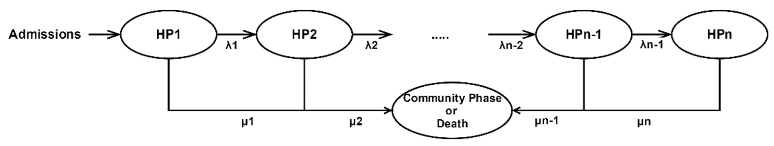
Figure 2.
Patient flow in the healthcare system.
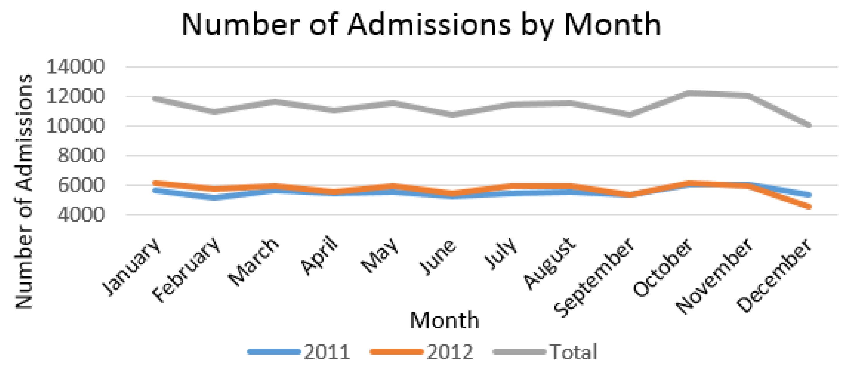
Figure 3.
Admissions by Day.
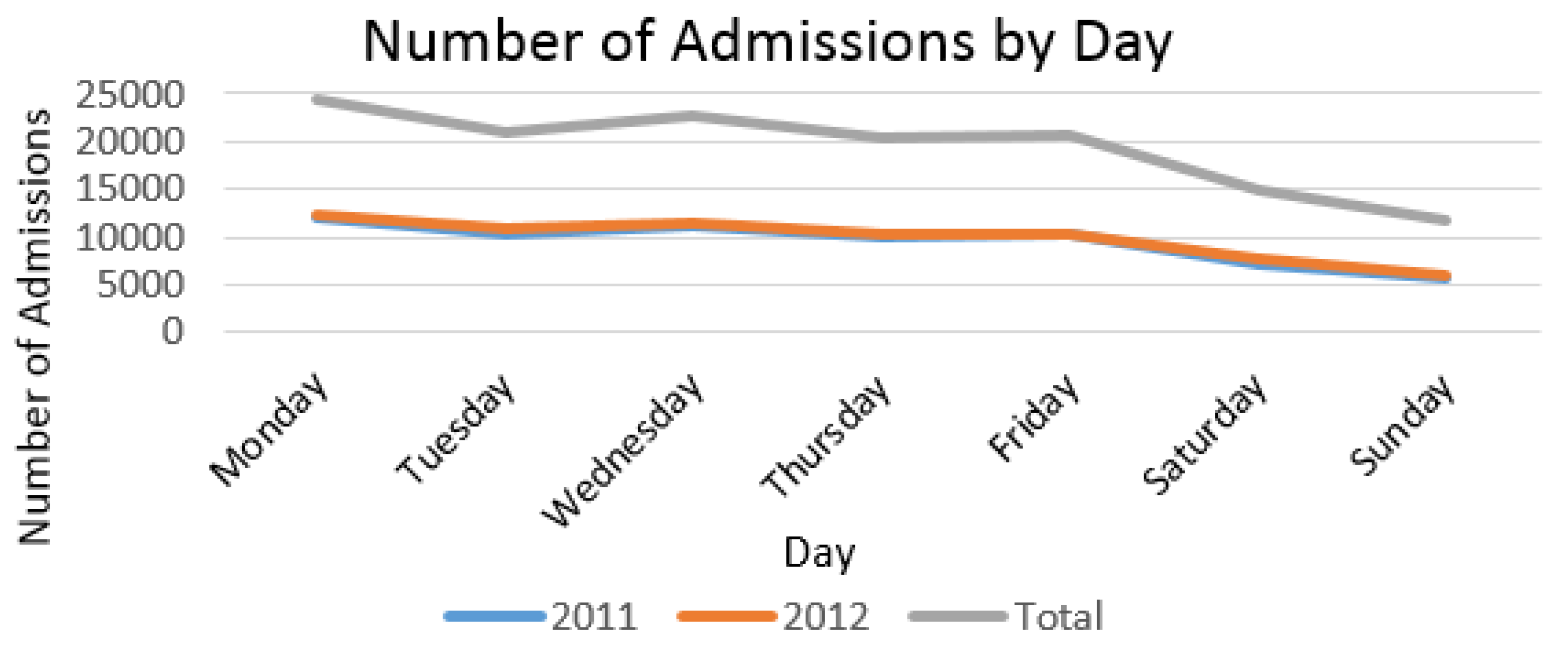
Figure 4.
Type of Admission by Day.
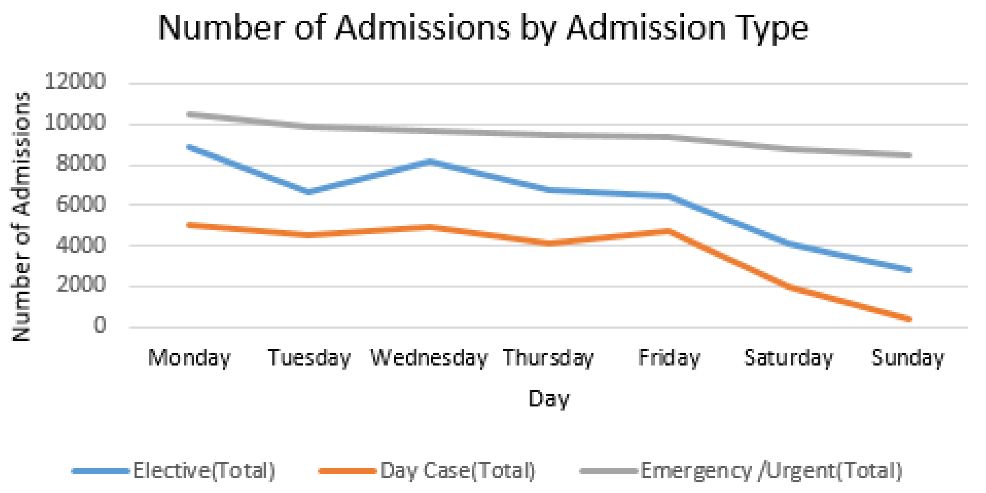
Figure 5.
Length of Stay Phase-Type Survival Tree related to personal characteristics.
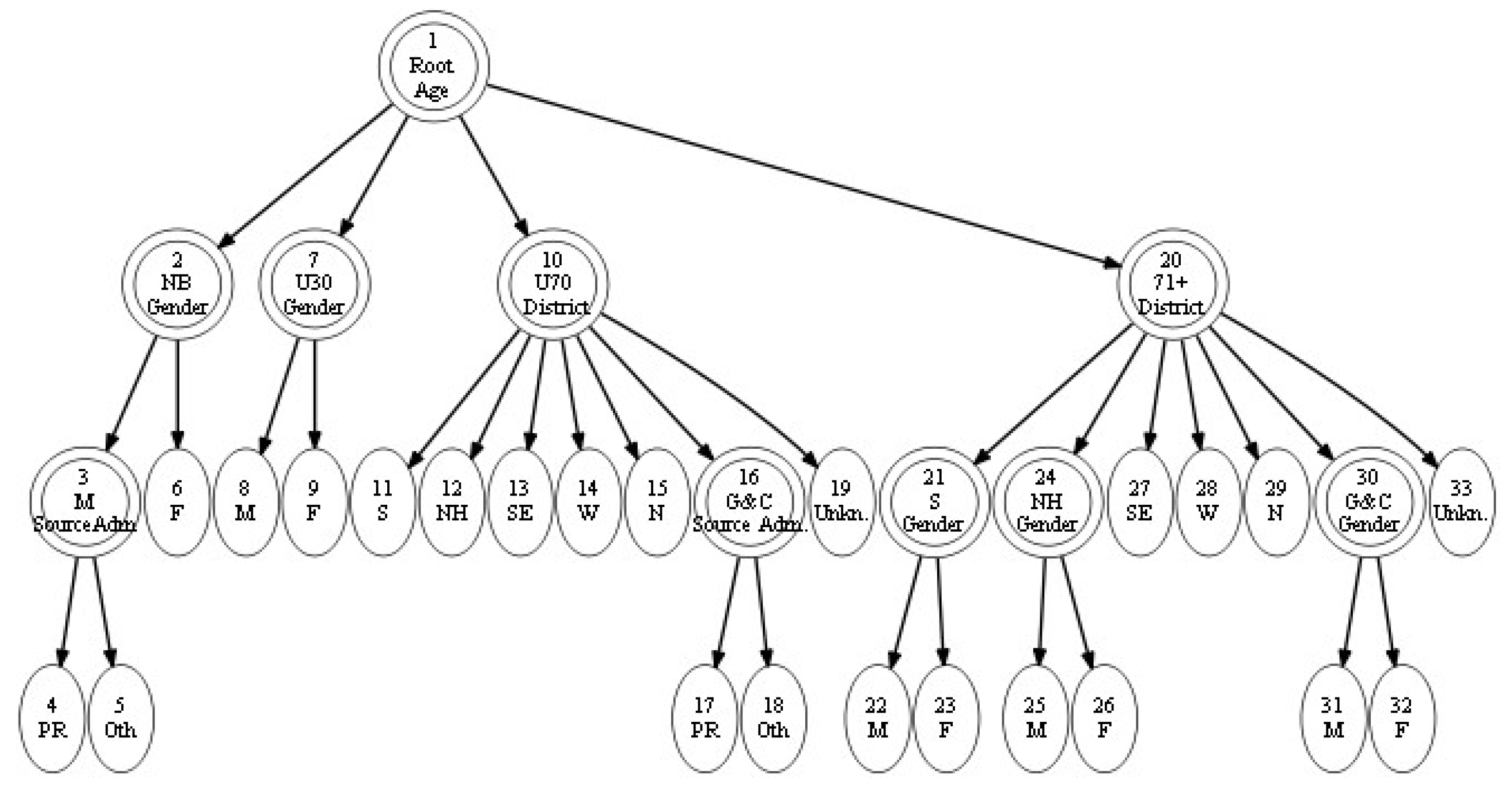
Figure 6.
Survival Function Plots for Length of Stay analysis related to Personal Characteristics.
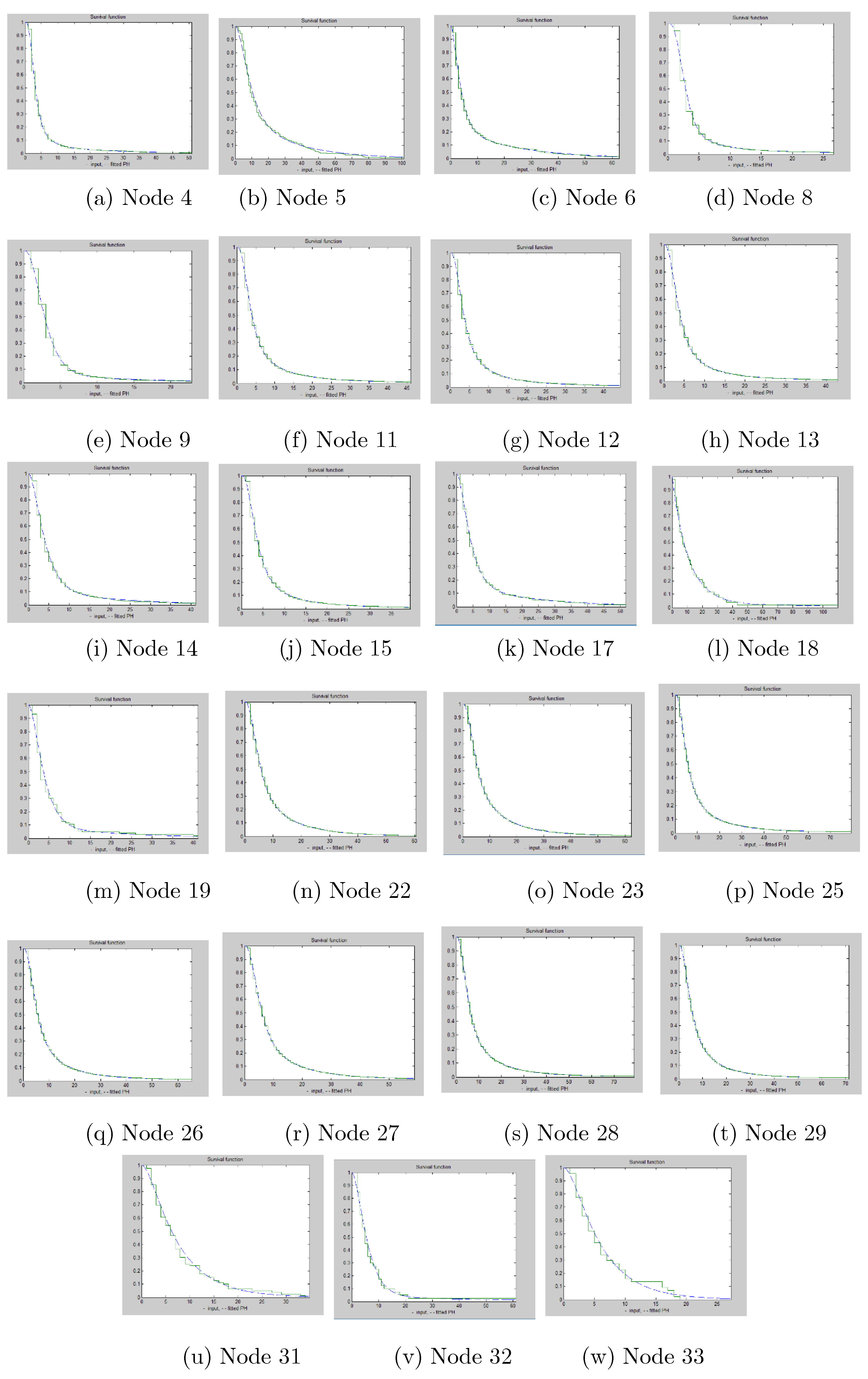
Figure 7.
Admission Phase-Type Survival Tree related to personal characteristics.
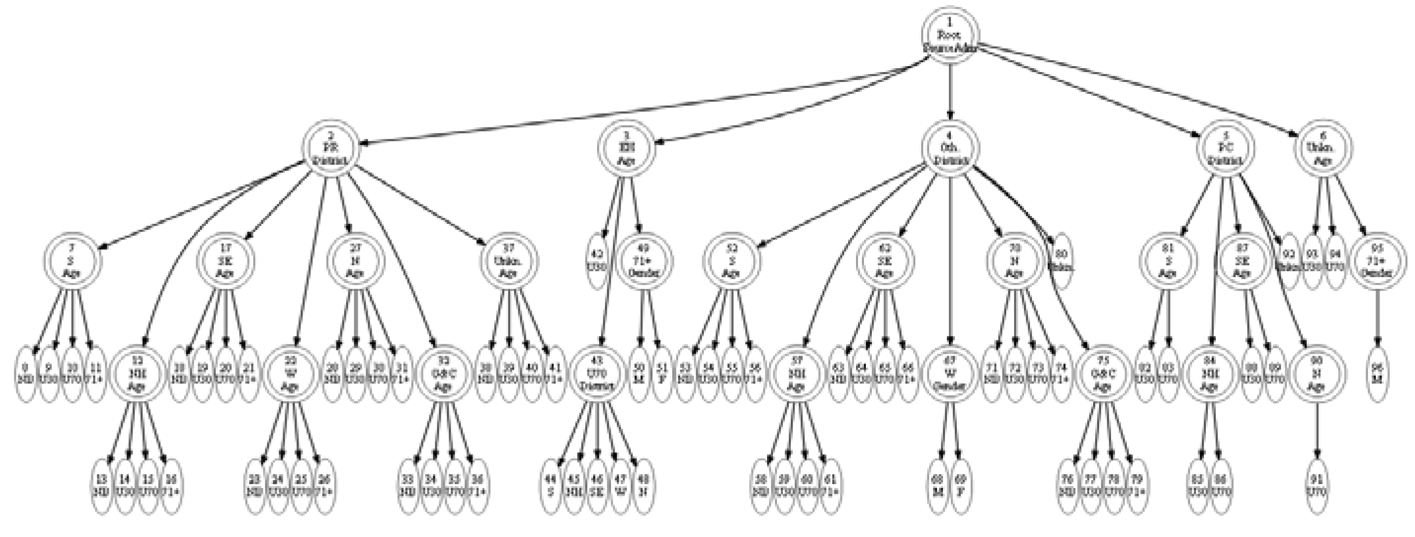

Table 1.
Admission Types.
| Admission Type |
Grp No |
No of Admissions |
Total LOS (Days) |
Average LOS (Days) |
|---|---|---|---|---|
| Elective/Planned procedure | 1 | 43 589 | 108 714 | 2.49 |
| Day Case | 2 | 25 748 | 2 856 | 0.11 |
| Emergency | 3 | 66 167 | 389 277 | 5.88 |
Table 2.
Daily and Monthly Admissions.
| Sun. | Mon. | Tue. | Wed. | Thur. | Fri. | Sat. | Total | |
|---|---|---|---|---|---|---|---|---|
| Jan. | 1135 | 2423 | 1897 | 1837 | 1630 | 1650 | 1250 | 11822 |
| Feb. | 989 | 1942 | 1663 | 2013 | 1585 | 1518 | 1202 | 10912 |
| Mar. | 917 | 1855 | 1799 | 2010 | 1941 | 1851 | 1258 | 11631 |
| Apr. | 999 | 2179 | 1634 | 1783 | 1580 | 1555 | 1305 | 11035 |
| May | 999 | 2064 | 1941 | 1994 | 1780 | 1621 | 1128 | 11527 |
| Jun. | 867 | 1835 | 1528 | 1888 | 1629 | 1731 | 1252 | 10730 |
| Jul. | 1113 | 2174 | 1873 | 1745 | 1528 | 1793 | 1222 | 11448 |
| Aug. | 849 | 2042 | 1779 | 2097 | 1802 | 1815 | 1112 | 11496 |
| Sept. | 934 | 1874 | 1623 | 1668 | 1756 | 1666 | 1189 | 10710 |
| Oct. | 973 | 2402 | 1947 | 2026 | 1683 | 1783 | 1394 | 12208 |
| Nov. | 946 | 1942 | 1971 | 2091 | 1891 | 1865 | 1278 | 11984 |
| Dec. | 894 | 1671 | 1404 | 1572 | 1469 | 1729 | 1262 | 10001 |
| Total | 11615 | 24403 | 21059 | 22724 | 20274 | 20577 | 14852 | 135504 |
Table 3.
Admissions by Covariate.
| Group | Group Number | Number of Admissions | Total LOS (Days) | Average LOS (Days) | ||
|---|---|---|---|---|---|---|
| Gender | Male (M) | 1 | 64347 | 237774 | 3.7 | |
| Female (F) | 2 | 71154 | 263066 | 3.7 | ||
| Unclassified (U) | 3 | 3 | 7 | 2.33 | ||
| Age | New Born (NB) | 1 | 2001 | 13602 | 6.8 | |
| Under 30 (U30) | 2 | 26675 | 61710 | 2.31 | ||
| Under 70 (U70) | 3 | 70972 | 213759 | 3.01 | ||
| Over70 (70+) | 4 | 35856 | 2117733 | 5.91 | ||
| District | South (S) | 1 | 30141 | 116659 | 3.87 | |
| Northern Harbour (NH) | 2 | 43544 | 163957 | 3.77 | ||
| South Eastern (SE) | 3 | 20140 | 70867 | 3.52 | ||
| Western (W) | 4 | 20231 | 68680 | 3.39 | ||
| North (N) | 5 | 18320 | 71210 | 3.89 | ||
| Gozo & Comino (G&C) | 2 | 2877 | 8402 | 2.92 | ||
| Unknown (Unkn.) | 7 | 251 | 1072 | 4.27 | ||
| Source Adm | Private Residence (PR) | 1 | 131486 | 467002 | 3.55 | |
| Elderly Home (EH) | 2 | 2153 | 17741 | 8.24 | ||
| Other (Oth.) | 3 | 1719 | 15565 | 9.05 | ||
| Police Custody (PC) | 7 | 121 | 432 | 3.57 | ||
| Unknown (Unkn.) | 8 | 25 | 107 | 4.28 |
Table 4.
Step 1: Splitting the root node.
| Group No (LEFT) | Group No (Right) | Phase (x) | Min WIC | Gain in WIC | Mean | Number of Patients | |
|---|---|---|---|---|---|---|---|
| -1 | 1 | 5 |
361646.8 00352 |
6.8833 36 |
66166 | ||
| (Gender) | Male (1) | 4 | 177934.678 409 |
6.8636 62 |
32534 | ||
| Female (2) | 5 | 183735.661 181 |
6.9023 68 |
33632 | |||
| Total |
361670.339 590 |
-23.539238 | 66166 | ||||
| (Age) | New Born(1) | 3 | 10012.7788 53 |
8.4770 89 |
1723 | ||
| Under 30 (2) | 3 | 61903.7200 90 |
3.9866 51 |
14448 | |||
| Under 70 (3) | 5 | 151714.199 007 |
6.2546 08 |
28783 | |||
| Over 70 (4) | 3 | 131504.220 027 |
9.5800 05 |
21212 | |||
| Total |
355134.917 977 |
6511.8823 75 |
66166 | ||||
| (District) | South(1) | 5 | 85076.4757 44 |
7.0394 28 |
15425 | ||
| Northern Harbour (2) | 8 | 117008.277 057 |
6.9202 93 |
21655 | |||
| North(3) | 8 | 51220.9755 15 |
6.6327 38 |
9560 | |||
| South Eastern (4) | 6 | 47328.3647 78 |
7.1001 95 |
8673 | |||
| Western (5) | 6 | 53183.5224 45 |
6.5479 29 |
10067 | |||
| Gozo & Comino (6) | 4 | 3414.70992 5 |
8.6470 70 |
561 | |||
| Unknown (7) | 3 | 1158.46334 9 |
5.5200 11 |
225 | |||
| Total |
358390.788 813 |
3256.0115 39 |
66166 | ||||
| (SourceAd) | Home/Private Residence (1) | 6 | 342853.702 690 |
6.8778 48 |
62768 | ||
| Home for the Elderly (2) | 6 | 10848.8042 71 |
7.4701 27 |
1925 | |||
| Other (3) | 6 | 7224.35563 7 |
6.3847 84 |
1354 | |||
| Police Custody (4) | 4 | 527.989474 | 5.9793 81 |
97 | |||
| Unknown (5) | 2 | 123.147744 | 5.8636 39 |
22 | |||
| Total |
361577.999 816 |
68.800536 | 66166 | ||||
Table 5.
Splitting of node 2 (newborn).
| Group No(LEFT) | Group No (Right) | Phase(x) | Min WIC | Gain in WIC | Mean LoS | Number of Patients | |
|---|---|---|---|---|---|---|---|
| AGE | |||||||
| NEWBORN | 10012.778853 | ||||||
| (NewBorn, Gender) | New Born(1) | Male (1) | 7 | 5671.189081 | 8.468910 | 981 | |
| Female (2) | 3 | 4328.550269 | 8.487877 | 742 | |||
| Total | 9999.739350 | 13.039503 | 1723 | ||||
| (NewBorn, District) | New Born (1) | South(1) | 4 | 1989.266679 | 6.852457 | 366 | |
| Northern Harbour (2) | 6 | 2930.781916 | 9.024242 | 495 | |||
| North(3) | 3 | 1766.753425 | 9.600010 | 290 | |||
| South Eastern (4) | 6 | 1379.362716 | 8.834041 | 235 | |||
| Western (5) | 3 | 1826.139737 | 8.422087 | 308 | |||
| Gozo & Comino (6) | 1 | 130.293698 | 6.681803 | 22 | |||
| Unknown (7) | 1 | 36.823822 | 4.285702 | 7 | |||
| Total | 10059.421993 | -46.643140 | 1723 | ||||
| (NewBorn, SourceAd) | New Born (1) | Home/Private Residence (1) | 6 | 5820.815591 | 5.087955 | 1262.000000 | |
| Home for the Elderly (2) | 0 | 0.000000 | 0.000000 | 0.000000 | |||
| Other (3) | 4 | 3476.917454 | 17.789126 | 460.000000 | |||
| Police Custody (4) | |||||||
| Unknown (5) | 0 | 0.000000 | 0.000000 | 0.000000 | |||
| Total | 9297.733045 | - | 1722.000000 |
Table 6.
Splitting of node 7 (under30).
| Group No(LEFT) | Group No (Right) | Phase(x) | Min WIC | Gain in WIC | Mean LoS | Number of Patients | |
|---|---|---|---|---|---|---|---|
| Under 30 | 61903.720090 | ||||||
| (Under30,Gender) | Under 30 (2) | Male (1) | 8 | 24762.357659 | 4.157465 | 6014 | |
| Female (2) | 4 | 34819.058665 | 3.864831 | 8434 | |||
| Total | 59581.416324 | 2322.303766 | 14448 | ||||
| (Under30,District) | Under 30 (2) | South(1) | 4 | 12229.294247 | 3.908124 | 3015 | |
| Northern Harbour (2) | 7 | 19064.333156 | 3.920145 | 4646 | |||
| North(3) | 8 | 10468.167480 | 4.010334 | 2516 | |||
| South Eastern (4) | 8 | 7760.544477 | 4.123213 | 1818 | |||
| Western (5) | 6 | 9248.253348 | 3.992421 | 2243 | |||
| Gozo & Comino (6) | 5 | 670.160344 | 5.035972 | 139 | |||
| Unknown (7) | 2 | 367.065126 | 5.098594 | 71 | |||
| Total | 59807.818178 | 2095.901912 | 14448 | ||||
| (Under30 SourceAd) | Under30 (2) | Home/Private Residence (1) | 5 | 59322.168631 | 3.993065 | 14280 | |
| Home for the Elderly (2) | 1 | 17.814737 | 2.249994 | 4 | |||
| Other (3) | 5 | 454.471483 | 3.509091 | 110 | |||
| Police Custody (4) | 2 | 203.869298 | 3.404259 | 47 | |||
| Unknown (5) | 1 | 33.103980 | 3.285708 | 7 | |||
| Total | 60031.428129 | 1872.291961 | 14448 |
Table 7.
Splitting of node 10 (under70).
| Group No(LEFT) | Group No (Right) | Phase(x) | Min WIC | Gain in WIC | Mean LoS | Number of Patients | |
|---|---|---|---|---|---|---|---|
| Under 70 | 151714.199007 | ||||||
| (Under70,Gender) | Under70 (3) | Male(1) | 8 | 83826.550005 | 6.427080 | 15908 | |
| Female(1) | 5 | 66625.781453 | 6.041493 | 12875 | |||
| Total | 150452.331458 | 1261.867549 | 28783 | ||||
| (Under70, District) | Under70(3) | South(1) | 8 | 36179.722530 | 6.491151 | 6839 | |
| Northern Harbour (2) | 7 | 47896.621672 | 6.245476 | 9231 | |||
| North(3) | 5 | 21792.241004 | 6.115920 | 4227 | |||
| South Eastern (4) | 4 | 19000.962563 | 6.234211 | 3642 | |||
| Western (5) | 5 | 22724.694230 | 5.925784 | 4460 | |||
| Gozo & Comino (6) | 3 | 1694.239739 | 8.551612 | 281 | |||
| Unknown (7) | 3 | 541.203201 | 5.747590 | 103 | |||
| Total | 149829.684939 | 1884.514068 | 28783 | ||||
| (Under70, SourceAd) | Under70 (3) | Home/Private Residence (1) | 5 | 147334.046566 | 6.187096 | 28057 | |
| Home for the Elderly (2) | 4 | 1106.978811 | 12.406056 | 165 | |||
| Other (3) | 3 | 2941.858154 | 8.160019 | 500 | |||
| Police Custody (4) | 2 | 233.070968 | 4.448993 | 49 | |||
| Unknown (5) | 1 | 74.800853 | 7.499985 | 12 | |||
| Total | 151690.755352 | 23.443655 | 28783 |
Table 8.
Splitting of node 20 (over70).
| Group No(LEFT) | Group No (Right) | Phase(x) | Min WIC | Gain in WIC | Mean LoS | Number of Patients | |
|---|---|---|---|---|---|---|---|
| Over 70 | 131504.220027 | ||||||
| (Over70, Gender) | Over 70 (4) | Male(1) | 8 | 58227.021014 | 9.111098 | 9631 | |
| Female(1) | 5 | 72557.524021 | 9.969958 | 11581 | |||
| Total | 130784.545035 | 21212 | |||||
| (Over70,District) | Over70 (4) | South(1) | 4 | 32111.561935 | 9.485891 | 5205 | |
| Northern Harbour (2) | 6 | 44822.046650 | 9.634491 | 7283 | |||
| North(3) | 5 | 15668.195104 | 9.491888 | 2527 | |||
| South Eastern (4) | 6 | 18437.143066 | 9.868703 | 2978 | |||
| Western (5) | 5 | 18559.234106 | 9.336389 | 3056 | |||
| Gozo & Comino (6) | 1 | 841.396961 | 12.411740 | 119 | |||
| Unknown (7) | 2 | 252.519962 | 6.477275 | 44 | |||
| Total | 130692.097784 | 21212 | |||||
| Over70, SourceAd) | Over70(4) | Home/Private Residence (1) | 5 | 118526.930185 | 9.570515 | 19169 | |
| Home for the Elderly (2) | 5 | 10955.926971 | 9.904898 | 1756 | |||
| Other (3) | 4 | 1686.065782 | 8.176068 | 284 | |||
| Police Custody (4) | 0 | 0.000000 | 0.000000 | 0 | |||
| Unknown (5) | 1 | 26.631132 | 12.999959 | 3 | |||
| Total | 131195.554070 | 21212 |
Table 9.
Splitting of node 3 (newborn, male).
| Group No(LEFT) | Group No (Right) | Phase(x) | Min WIC | Gain in WIC | Mean LoS | Number of Patients | |
|---|---|---|---|---|---|---|---|
| (NewBorn, Gender) | 9999.739350 | ||||||
| Male | 5671.189081 | ||||||
| (Male, District) | Male (1) | South(1) | 4 | 1254.339181 | 7.906975 | 215 | |
| Northern Harbour (2) | 5 | 1581.650098 | 7.764708 | 272 | |||
| North(3) | 3 | 1045.542060 | 10.64672 | 167 | |||
| South Eastern (4) | 4 | 754.318483 | 9.776922 | 130 | |||
| Western (5) | 4 | 945.469803 | 6.289771 | 176 | |||
| Gozo & Comino (6) | 1 | 135.295601 | 18.235257 | 17 | |||
| Unknown (7) | 1 | 27.446517 | 7.499974 | 4 | |||
| Total | 5744.061743 | -72.872662 | 981 | ||||
| (Male, Source Adm) | Male (1) | Home/Private Residence (1) | 8 | 3245.521267 | 5.026874 | 707 | |
| Home for the Elderly (2) | 0 | 0.000000 | 0 | 0 | |||
| Other (3) | 3 | 2062.865571 | 17.35037 | 274 | |||
| Police Custody (4) | 0 | 0.000000 | 0 | 0 | |||
| Unknown (5) | 0 | 0.000000 | 0 | 0 | |||
| Total | 5308.386838 | 362.802243 | 981 |
Table 10.
Splitting of node 4 (newborn, female).
| Group No(LEFT) | Group No (Right) | Phase(x) | Min WIC | Gain in WIC | Mean LoS | Number of Patients | |
|---|---|---|---|---|---|---|---|
| (NewBorn, Gender) | 9999.739350 | ||||||
| Female | 4328.550269 | ||||||
| (Female, District) | Female (2) | South(1) | 4 | 855.680118 | 7.993377 | 151 | |
| Northern Harbour (2) | 3 | 1260.685410 | 7.25561 | 223 | |||
| North(3) | 3 | 784.207481 | 10.731718 | 123 | |||
| South Eastern (4) | 3 | 635.191831 | 8.095251 | 105 | |||
| Western (5) | 3 | 805.786816 | 9.4091 | 132 | |||
| Gozo & Comino (6) | 1 | 35.389634 | 9.599978 | 5 | |||
| Unknown (7) | 1 | 20.039458 | 4.333319 | 3 | |||
| Total | 4396.980748 | -68.430479 | 742 | ||||
| (Female, Source Adm) | Female (2) | Home/Private Residence (1) | 6 | 2597.152945 | 5.165765 | 555 | |
| Home for the Elderly (2) | 0 | 0.000000 | 0 | 0 | |||
| Other (3) | 3 | 1445.680286 | 18.435491 | 186 | |||
| Police Custody (4) | 0 | 0.000000 | 0 | 0 | |||
| Unknown (5) | 1 | ||||||
| Total | 4042.833231 | - | 742 |
Table 11.
Splitting of node 8 (under30, male).
| Group No(LEFT) | Group No (Right) | Phase(x) | Min WIC | Gain in WIC | Mean LoS | Number of Patients | |
|---|---|---|---|---|---|---|---|
| (Under30,Gender) | 59581.416324 | ||||||
| Male | 24762.357659 | ||||||
| (Male, District) | Male (1) | South(1) | 4 | 5015.288548 | 3.938272 | 1215 | |
| Northern Harbour (2) | 7 | 7842.125327 | 3.886901 | 1901 | |||
| North(3) | 4 | 4443.013215 | 4.152089 | 1052 | |||
| South Eastern (4) | 4 | 3191.036908 | 4.158877 | 749 | |||
| Western (5) | 5 | 4106.294365 | 3.878392 | 995 | |||
| Gozo & Comino (6) | 4 | 301.828482 | 5.65574 | 61 | |||
| Unknown (7) | 7 | 219.464227 | 5.219529 | 41 | |||
| Total | 25119.051072 | -356.693413 | 6014 | ||||
| (Male, Source Adm) | Male (1) | Home/Private Residence (1) | 5 | 24609.783767 | 4.008127 | 5905 | |
| Home for the Elderly (2) | 8 | 25.784190 | 2 | 2 | |||
| Other (3) | 3 | 298.838775 | 3.514286 | 70 | |||
| Police Custody (4) | 2 | 136.570976 | 3.343766 | 32 | |||
| Unknown (5) | 1 | 23.068196 | 2.800001 | 5 | |||
| Total | 25094.045904 | -331.688245 | 6014 | ||||
Table 12.
Splitting of node 9 (under30, female).
| Group No(LEFT) | Group No (Right) | Phase(x) | Min WIC | Gain in WIC | Mean LoS | Number of Patients | |
|---|---|---|---|---|---|---|---|
| (Under30,Gender) | 59581.416324 | ||||||
| Female | 34819.058665 | ||||||
| (Female, District) | Female (2) | South(1) | 4 | 7249.484970 | 3.887779 | 1800 | |
| Northern Harbour (2) | 7 | 11294.974230 | 3.94317 | 2745 | |||
| North(3) | 8 | 6076.287810 | 3.90847 | 1464 | |||
| South Eastern (4) | 4 | 4624.380902 | 4.098221 | 1069 | |||
| Western (5) | 5 | 5172.844942 | 4.083332 | 1248 | |||
| Gozo & Comino (6) | 4 | 391.544707 | 5.01282 | 78 | |||
| Unknown (7) | 2 | 157.062802 | 4.933335 | 30 | |||
| Total | 34966.580363 | -147.521698 | 8434 | ||||
| (Female, Source Adm) | Female (2) | Home/Private Residence (1) | 7 | 34765.233298 | 3.982446 | 8375 | |
| Home for the Elderly (2) | 8 | 24.488864 | 2.5 | 2 | |||
| Other (3) | 2 | 174.300341 | 3.500003 | 40 | |||
| Police Custody (4) | 1 | 70.391080 | 3.53332 | 15 | |||
| Unknown (5) | 8 | 29.186046 | 4.500001 | 2 | |||
| Total | 35063.599629 | -244.540964 | 8434 |
Table 13.
Splitting of node 11 (under70, South).
| Group No(LEFT) | Group No (Right) | Phase(x) | Min WIC | Gain in WIC | Mean LoS | Number of Patients | |
|---|---|---|---|---|---|---|---|
| Under70, South | 36179.722530 | ||||||
| (South,Gender) | South(1) | Male(1) | 7 | 21259.453641 | 6.658919 | 3958 | |
| Female (2) | 4 | 15123.963246 | 6.260690 | 2881 | |||
| Total | 36383.416887 | 6839 | |||||
| (South, SourceAd) | South(1) | Home/Private Residence (1) | 7 | 35068.570609 | 6.426725 | 6653 | |
| Home for the Elderly (2) | 2 | 436.714463 | 11.140626 | 64 | |||
| Other (3) | 3 | 511.342182 | 8.730343 | 89 | |||
| Police Custody (4) | 2 | 146.623489 | 4.225823 | 31 | |||
| Unknown (5) | 8 | 28.374166 | 7.499998 | 2 | |||
| Total | 36191.624909 | 6839 |
Table 14.
Splitting of node 12 (under70, Northern Harbour).
| Group No(LEFT) | Group No (Right) | Phase(x) | Min WIC | Gain in WIC | Mean LoS | Number of Patients | |
|---|---|---|---|---|---|---|---|
| Under70, Northern Harbor | 47896.621672 | ||||||
| (Northern Harbour, Gender) | Northern Harbour (2) | Male(1) | 7 | 25791.494476 | 6.431719 | 4899 | |
| Female(2) | 4 | 22470.801040 | 6.034865 | 4332 | |||
| Total | 48262.295516 | 9231 | |||||
| (Northern Harbour, Source Ad) | Northern Harbout | Home/Private Residence (1) | 7 | 46877.911687 | 6.191394 | 9065 | |
| Home for the Elderly (2) | 3 | 248.362703 | 13.861127 | 36 | |||
| Other (3) | 3 | 737.934459 | 7.959033 | 122 | |||
| Police Custody (4) | 3 | 29.896774 | 8.400001 | 3 | |||
| Unknown (5) | 1 | 34.054318 | 8.399973 | 5 | |||
| Total | 47928.159941 | 9231 |
Table 15.
Splitting of node 13 (under70, North).
| Group No(LEFT) | Group No (Right) | Phase(x) | Min WIC | Gain in WIC | Mean LoS | Number of Patients | |
|---|---|---|---|---|---|---|---|
| Under70, North | 21792.241004 | ||||||
| (North, Gender) | North | Male | 5 | 12264.120596 | 6.121713 | 2358 | |
| Female | 7 | 9613.629943 | 6.108613 | 1869 | |||
| Total | 21877.750539 | 4227 | |||||
| (North, Source Ad) | North | Home/Private Residence (1) | 7 | 21353.617068 | 6.051817 | 4149 | |
| Home for the Elderly (2) | 2 | 111.206699 | 22.214268 | 14 | |||
| Other (3) | 2 | 304.696250 | 7.313725 | 51 | |||
| Police Custody (4) | 1 | 59.829022 | 4.999993 | 11 | |||
| Unknown (5) | 8 | 23.024782 | 2.000000 | 2 | |||
| Total | 21852.373821 | 4227 |
Table 16.
Splitting of node 14 (under70, South Eastern).
| Group No(LEFT) | Group No (Right) | Phase(x) | Min WIC | Gain in WIC | Mean LoS | Number of Patients | |
|---|---|---|---|---|---|---|---|
| Under 70, South Eastern | 19000.962563 | ||||||
| (South Eastern, Gender) | South Eastern | Male | 7 | 10563.552355 | 6.486868 | 1980 | |
| Female | 8 | 8504.979825 | 5.933213 | 1662 | |||
| Total | 19068.532180 | 3642 | |||||
| (South Eastern, Source Ad) | South Eastern | Home/Private Residence (1) | 6 | 18234.008928 | 6.209596 | 3502 | |
| Home for the Elderly (2) | 1 | 116.581524 | 8.722206 | 18 | |||
| Other (3) | 4 | 672.250660 | 6.570248 | 121 | |||
| Police Custody (4) | 0 | 0.000000 | 0.000000 | 0 | |||
| Unknown (5) | 5 | 2.153548 | 7.000001 | 1 | |||
| Total | 19024.994660 | 3642 | |||||
Table 17.
Splitting of node 15 (under70, Western).
| Group No(LEFT) | Group No (Right) | Phase(x) | Min WIC | Gain in WIC | Mean LoS | Number of Patients | |
|---|---|---|---|---|---|---|---|
| Under70, Western | 22724.694230 | ||||||
| (Western, Gender) | Western | Male | 5 | 12873.941204 | 6.140891 | 2470 | |
| Female | 7 | 9915.033235 | 5.658793 | 1990 | |||
| Total | 22788.974439 | 4460 | |||||
| (Western, Source Ad) | Western | Home/Private Residence (1) | 7 | 22142.923818 | 5.865305 | 4358 | |
| Home for the Elderly (2) | 3 | 223.497916 | 11.121216 | 33 | |||
| Other (3) | 3 | 372.982708 | 7.333353 | 63 | |||
| Police Custody (4) | 1 | 22.902645 | 4.249986 | 4 | |||
| Unknown (5) | 8 | 32.464970 | 10.999995 | 2 | |||
| Total | 22794.772057 | 4460 | |||||
Table 18.
Splitting of node 16 (under70, Gozo&Comino).
| Group No(LEFT) | Group No (Right) | Phase(x) | Min WIC | Gain in WIC | Mean LoS | Number of Patients | |
|---|---|---|---|---|---|---|---|
| Under70, Gozo&Comino | 1694.239739 | ||||||
| (Gozo&Comino, Gender) | G&C | Male | 3 | 1070.155036 | 8.477530 | 178 | |
| Female | 3 | 635.879929 | 8.679620 | 103 | |||
| Total | 1706.034965 | 281 | |||||
| (Gozo&Comino, Source Ad) | G&C | Home/Private Residence (1) | 3 | 1314.692761 | 7.445427 | 229 | |
| Home for the Elderly (2) | 0 | 0.000000 | 0.000000 | 0 | |||
| Other (3) | 2 | 376.458138 | 13.423041 | 52 | |||
| Police Custody (4) | 0 | 0.000000 | 0.000000 | 0 | |||
| Unknown (5) | 0 | 0.000000 | 0.000000 | 0 | |||
| Total | 1691.150899 | 281 | |||||
Table 19.
Splitting of node 19 (under70, Unknown).
| Group No(LEFT) | Group No (Right) | Phase(x) | Min WIC | Gain in WIC | Mean LoS | Number of Patients | |
|---|---|---|---|---|---|---|---|
| Under70, Unknown | 541.203201 | ||||||
| (Unknown, Gender) | Unknown | Male | 3 | 364.431958 | 6.476937 | 65 | |
| Female | 3 | 187.188527 | 4.500013 | 38 | |||
| Total | 551.620485 | 103 | |||||
| (Unknown, Source Ad) | Unknown | Home/Private Residence (1) | 3 | 533.427248 | 5.821799 | 101 | |
| Home for the Elderly (2) | 0 | 0.000000 | 0.000000 | 0 | |||
| Other (3) | 8 | 26.046172 | 2.000000 | 2 | |||
| Police Custody (4) | 0 | 0.000000 | 0.000000 | 0 | |||
| Unknown (5) | 0 | 0.000000 | 0.000000 | 0 | |||
| Total | 559.473420 | 103 |
Table 20.
Splitting of node 21 (over70, South).
| Group No(LEFT) | Group No (Right) | Phase(x) | Min WIC | Gain in WIC | Mean LoS | Number of Patients | |
|---|---|---|---|---|---|---|---|
| Over70,District | 130692.097784 | ||||||
| Over70, South | 32111.561935 | ||||||
| (South,Gender) | South(1) | Male(1) | 7 | 14714.295158 | 9.105985 | 2406 | |
| Female (2) | 7 | 17247.234115 | 9.423006 | 2799 | |||
| Total | 31961.529273 | 5205 | |||||
| (South, SourceAd) | South(1) | Home/Private Residence (1) | 4 | 29580.700863 | 9.305313 | 4792 | |
| Home for the Elderly (2) | 4 | 2225.745864 | 9.251395 | 358 | |||
| Other (3) | 2 | 320.023091 | 6.927273 | 55 | |||
| Police Custody (4) | 0 | 0.000000 | 0.000000 | 0 | |||
| Unknown (5) | 0 | 0.000000 | 0.000000 | 0 | |||
| Total | 32126.469818 | 5205 |
Table 21.
Splitting of node 24 (over70, Northern Harbour).
| Group No(LEFT) | Group No (Right) | Phase(x) | Min WIC | Gain in WIC | Mean LoS | Number of Patients | |
|---|---|---|---|---|---|---|---|
| Over70, Northern Harbor | 44822.046650 | ||||||
| (Northern Harbour, Gender) | Northern Harbour (2) | Male(1) | 7 | 20773.565966 | 9.957635 | 3352 | |
| Female(2) | 8 | 23927.621456 | 9.284152 | 3931 | |||
| Total | 44701.187422 | 7283 | |||||
| (Northern Harbour, Source Ad) | Northern Harbout | Home/Private Residence (1) | 4 | 41422.992605 | 9.604185 | 6710 | |
| Home for the Elderly (2) | 4 | 3049.111549 | 9.784550 | 492 | |||
| Other (3) | 4 | 466.389961 | 7.604933 | 81 | |||
| Police Custody (4) | 0 | 0.000000 | 0.000000 | 0 | |||
| Unknown (5) | 0 | 0.000000 | 0.000000 | 0 | |||
| Total | 44938.494115 | 7283 |
Table 22.
Splitting of node 27 (over70, North).
| Group No(LEFT) | Group No (Right) | Phase(x) | Min WIC | Gain in WIC | Mean LoS | Number of Patients | |
|---|---|---|---|---|---|---|---|
| Over70, North | 15668.195104 | ||||||
| (North, Gender) | North | Male | 7 | 6901.967381 | 9.851752 | 1113 | |
| Female | 8 | 9050.657193 | 10.528292 | 1414 | |||
| Total | 15952.624574 | 2527 | |||||
| (North, Source Ad) | North | Home/Private Residence (1) | 4 | 14779.181823 | 10.256322 | 2337 | |
| Home for the Elderly (2) | 3 | 1031.121664 | 10.030494 | 164 | |||
| Other (3) | 1 | 169.959218 | 9.153838 | 26 | |||
| Police Custody (4) | 0 | 0.000000 | 0.000000 | 0 | |||
| Unknown (5) | 0 | 0.000000 | 0.000000 | 0 | |||
| Total | 15980.262705 | 2527 |
Table 23.
Splitting of node 28 (over70, South Eastern).
| Group No(LEFT) | Group No (Right) | Phase(x) | Min WIC | Gain in WIC | Mean LoS | Number of Patients | |
|---|---|---|---|---|---|---|---|
| Under 70, South Eastern | 18437.143066 | ||||||
| (South Eastern, Gender) | South Eastern | Male | 6 | 7767.242350 | 9.843978 | 1237 | |
| Female | 8 | 10778.677902 | 9.696152 | 1741 | |||
| Total | 18545.920252 | 2978 | |||||
| (South Eastern, Source Ad) | South Eastern | Home/Private Residence (1) | 6 | 15927.026988 | 9.650990 | 2573 | |
| Home for the Elderly (2) | 3 | 2211.483030 | 10.540473 | 346 | |||
| Other (3) | 2 | 372.784988 | 9.578948 | 57 | |||
| Police Custody (4) | 0 | 0.000000 | 0.000000 | 0 | |||
| Unknown (5) | 8 | 34.289246 | 16.500001 | 2 | |||
| Total | 18545.584252 | 2978 |
Table 24.
Splitting of node 29 (over70, Western).
| Group No(LEFT) | Group No (Right) | Phase(x) | Min WIC | Gain in WIC | Mean LoS | Number of Patients | |
|---|---|---|---|---|---|---|---|
| Over70, Western | 18559.234106 | ||||||
| (Western, Gender) | Western | Male | 7 | 8720.229605 | 9.524345 | 1417 | |
| Female | 4 | 10089.835560 | 9.329470 | 1639 | |||
| Total | 18810.065165 | 3056 | |||||
| (Western, Source Ad) | Western | Home/Private Residence (1) | 6 | 16036.719389 | 9.299390 | 2632 | |
| Home for the Elderly (2) | 5 | 2537.928683 | 10.045568 | 395 | |||
| Other (3) | 1 | 198.190740 | 12.035684 | 28 | |||
| Police Custody (4) | 0 | 0.000000 | 0.000000 | 0 | |||
| Unknown (5) | 1 | ||||||
| Total | 18772.838812 | 3056 |
Table 25.
Splitting of node 30 (over70, Gozo&Comino).
| Group No(LEFT) | Group No (Right) | Phase(x) | Min WIC | Gain in WIC | Mean LoS | Number of Patients | |
|---|---|---|---|---|---|---|---|
| Over70, Gozo&Comino | 841.396961 | ||||||
| (Gozo&Comino, Gender) | G&C | Male | 2 | 484.147245 | 8.088608 | 79 | |
| Female | 3 | 243.881774 | 8.025018 | 40 | |||
| Total | 728.029019 | 119 | |||||
| (Gozo&Comino, Source Ad) | G&C | Home/Private Residence (1) | 2 | 531.656682 | 9.120484 | 83 | |
| Home for the Elderly (2) | 1 | ||||||
| Other (3) | 2 | 183.888567 | 5.600017 | 35 | |||
| Police Custody (4) | 0 | 0.000000 | 0.000000 | 0 | |||
| Unknown (5) | 0 | 0.000000 | 0.000000 | 0 | |||
| Total | 715.545249 | 119 | |||||
Table 26.
Splitting of node 33 (over70, Unknown).
| Group No(LEFT) | Group No (Right) | Phase(x) | Min WIC | Gain in WIC | Mean LoS | Number of Patients | |
|---|---|---|---|---|---|---|---|
| Over70, Unknown | 252.519962 | ||||||
| (Unknown, Gender) | Unknown | Male | 3 | 173.278569 | 11.222235 | 27 | |
| Female | 1 | 94.360517 | 5.470570 | 17 | |||
| Total | 267.639086 | 44 | |||||
| (Unknown, Source Ad) | Unknown | Home/Private Residence (1) | 3 | 253.940100 | 9.238111 | 42 | |
| Home for the Elderly (2) | 0 | 0.000000 | 0.000000 | 0 | |||
| Other (3) | 8 | 28.818760 | 4.000000 | 2 | |||
| Police Custody (4) | 0 | 0.000000 | 0.000000 | 0 | |||
| Unknown (5) | 0 | 0.000000 | 0.000000 | 0 | |||
| Total | 282.758860 | 44 |
Table 27.
Step 1: Splitting the root node.
| (1, Number Of Admissions) | 1 | 8 | 7847.1116 | 186.6491 | 721 | 7847.1116 | ||
| (Gender, Nr of Adm) | Male(1) | 8 | 6797.0617 | 88.6602 | 721 | 3398.5308 | ||
| Female(2) | 8 | 6960.8298 | 97.9847 | 721 | 3480.4149 | |||
| Total | 13757.8914 | 6878.9457 | 968.1658 | |||||
| (Age, Nr of Adm) | New Born (1) | 3 | 2430.8080 | 2.9745 | 667 | 607.7020 | ||
| Under 30(2) | 8 | 5529.8060 | 36.6685 | 721 | 1382.4515 | |||
| Under 70 (3) | 8 | 7111.5218 | 97.7795 | 721 | 1777.8805 | |||
| Over 71 (4) | 8 | 5922.6184 | 49.4494 | 721 | 1480.6546 | |||
| Total | 20994.7541 | 5248.6885 | 2598.4230 | |||||
| (District, Nr of Adm) | South(1) | 8 | 5775.6090 | 41.5312 | 721 | 825.0870 | ||
| Northern Harbour (2) | 8 | 6256.1519 | 59.9944 | 721 | 893.7360 | |||
| North(3) | 8 | 5316.1594 | 27.8488 | 721 | 759.4513 | |||
| South Eastern (4) | 8 | 5181.7809 | 25.2441 | 721 | 740.2544 | |||
| Western (5) | 8 | 5280.4273 | 27.7240 | 721 | 754.3468 | |||
| Gozo & Comino (6) | 3 | 3044.6887 | 4.2870 | 669 | 434.9555 | |||
| Unknown (7) | 6 | 341.3544 | 1.5000 | 158 | 48.7649 | |||
| Total | 31196.1717 | 4456.5960 | 3390.5156 | |||||
| (SourceAd, Nr of Adm) | Home/Private Residence (1) | 8 | 7818.1469 | 181.1082 | 721 | 1563.6294 | ||
| Home for the Elderly (2) | 3 | 2590.5717 | 3.1640 | 677 | 518.1143 | |||
| Other (3) | 4 | 2210.5691 | 2.6661 | 641 | 442.1138 | |||
| Police Custody (4) | 6 | 145.7583 | 1.2143 | 98 | 29.1517 | |||
| Unknown (5) | 3 | 42.2021 | 1.1905 | 21 | 8.4404 | |||
| Total | 12807.2481 | 2561.4496 | 5285.6619 | |||||
Table 28.
Step 2: Splitting node 2(Home/Private Residence).
| Group Number (Left) | Group Number (Right) | Phase | WIC | Mean | Number of Records | Average WIC | WIC Gain | |
|---|---|---|---|---|---|---|---|---|
| (SourceAd, Nr of Adm) | 12807.248112 | 0 | 2561.449622 | |||||
| Home/Private Residence (1) | 7818.146859 | 721 | 1563.629372 | |||||
| (Home, Gender) | Home | Male | 8 | 3825.276337 | 14.298197 | 721 | 382.5276337 | |
| Female | 8 | 3840.042543 | 14.511790 | 721 | 384.0042543 | |||
| Total | 7665.318880 | 766.531888 | 797.097484 | |||||
| (Home,Age) | Home | New Born | 5 | 1515.578455 | 1.945993 | 574 | 75.77892275 | |
| Under30 | 8 | 3125.114139 | 8.377254 | 721 | 156.255707 | |||
| Under70 | 8 | 3275.132289 | 9.932039 | 721 | 163.7566145 | |||
| Over 70 | 8 | 3164.530383 | 8.952843 | 721 | 158.2265192 | |||
| Total | 11080.355266 | 554.0177633 | 1009.611609 | |||||
| (Home, Locality) | Home | South(1) | 8 | 2623.259152 | 6.278779 | 721 | 74.95026149 | |
| Northern Harbour (2) | 8 | 2634.257255 | 6.278779 | 721 | 75.264493 | |||
| North(3) | 8 | 2546.221529 | 5.332871 | 721 | 72.74918654 | |||
| South Eastern (4) | 8 | 2517.560067 | 5.040910 | 721 | 71.93028763 | |||
| Western (5) | 8 | 2537.265545 | 5.391123 | 721 | 72.49330129 | |||
| Gozo & Comino (6) | 8 | 420.759504 | 1.256021 | 332 | 12.02170011 | |||
| Unknown (7) | 6 | 236.872569 | 1.345865 | 133 | 6.767787686 | |||
| Total | 13516.195621 | 386.1770177 | 1177.452354 |
Table 29.
Step 2: Splitting node 3(Home for the elderly).
| Group Number (Left) | Group Number (Right) | Phase | WIC | Mean | Number of Records | Average WIC | WIC Gain | |
|---|---|---|---|---|---|---|---|---|
| Home for the Elderly (2) | 2590.5717 | 721 | 518.1143 | |||||
| (Home for the elderly, Gender) | Home for the elderly | Male | 7 | 680.2011 | 1.4521 | 376 | 68.0201 | |
| Female | 4 | 1509.5300 | 1.8920 | 602 | 150.9530 | |||
| Total | 2189.7310 | 218.9731 | 299.1412 | |||||
| (Home for the elderly,Age) | Home for the elderly | New Born | 0 | 0.0000 | 0.0000 | 0 | 0.0000 | |
| Under30 | 1 | 11.3273 | 1.0000 | 4 | 0.5664 | |||
| Under70 | 8 | 121.5060 | 1.1103 | 145 | 6.0753 | |||
| Over 70 | 4 | 2004.0645 | 2.3493 | 647 | 100.2032 | |||
| Total | 2136.8978 | 106.8449 | 411.2695 | |||||
| (Home for the elderly, Locality) | Home for the elderly | South(1) | 8 | 307.0443 | 1.1804 | 316 | 8.7727 | |
| Northern Harbour (2) | 8 | 400.0539 | 1.2276 | 369 | 11.4301 | |||
| North(3) | 8 | 107.1798 | 1.0909 | 154 | 3.0623 | |||
| South Eastern (4) | 8 | 226.8566 | 1.1502 | 273 | 6.4816 | |||
| Western (5) | 8 | 254.9713 | 1.1498 | 327 | 7.2849 | |||
| Gozo & Comino (6) | 1 | bad wic | ||||||
| Unknown (7) | 0 | 0.0000 | 0.0000 | 0 | 0.0000 | |||
Table 30.
Step 2: Splitting node 4(Other source of admission).
| Group Number (Left) | Group Number (Right) | Phase | WIC | Mean | Number of Records | Average WIC | WIC Gain | |
|---|---|---|---|---|---|---|---|---|
| Other (3) | 2210.5691 | 442.1138 | ||||||
| (Other, Gender) | Other | Male | 7 | 989.2221 | 1.6151 | 465 | 98.9222 | |
| Female | 8 | 653.6929 | 1.4282 | 376 | 65.3693 | |||
| Total | 1642.9149 | 164.2915 | 277.8223 | |||||
| (Other,Age) | Other | New Born | 8 | 457.0267 | 1.3175 | 315 | 22.8513 | |
| Under30 | 8 | 81.0688 | 1.0792 | 101 | 4.0534 | |||
| Under70 | 8 | 540.1501 | 1.3188 | 367 | 27.0075 | |||
| Over 70 | 8 | 306.4893 | 1.2727 | 220 | 15.3245 | |||
| Total | 1384.7350 | 69.2367 | 372.8771 | |||||
| (Other, Locality) | Other | South(1) | 8 | 163.8176 | 1.1216 | 222 | 4.6805 | |
| Northern Harbour (2) | 8 | 365.7543 | 1.2694 | 271 | 10.4501 | |||
| North(3) | 8 | 126.2427 | 1.1154 | 156 | 3.6069 | |||
| South Eastern (4) | 8 | 172.8283 | 1.1315 | 213 | 4.9380 | |||
| Western (5) | 8 | 107.5059 | 1.0933 | 150 | 3.0716 | |||
| Gozo & Comino (6) | 8 | 90.2080 | 1.0900 | 100 | 2.5774 | |||
| Unknown (7) | 1 | 16.3980 | 1.1667 | 6 | 0.4685 | |||
| Total | 1042.7548 | 29.7930 | 412.3208 |
Table 31.
Step 2: Splitting node 5(Police Custody).
| Group Number (Left) | Group Number (Right) | Phase | WIC | Mean | Number of Records | Average WIC | WIC Gain | |
|---|---|---|---|---|---|---|---|---|
| Police Custody (4) | 145.7583 | 0 | 29.1517 | |||||
| (Police Custody, Gender) | Police Custody | Male | 6 | 73.9991 | 1.1148 | 61 | 7.3999 | |
| Female | 3 | 35.2291 | 1.0455 | 22 | 3.5229 | |||
| Total | 109.2281 | 10.9228 | 18.2289 | |||||
| (Police Custody,Age) | Police Custody | New Born | 1 | bad wic | ||||
| Under30 | 5 | 48.9482 | 1.0476 | 42 | 2.4474 | |||
| Under70 | 6 | 45.1786 | 1.0222 | 45 | 2.2589 | |||
| Over 70 | 0 | 0.0000 | 0.0000 | 0 | 0.0000 | |||
| Total | 94.1268 | |||||||
| (Police Custody, Locality) | Police Custody | South(1) | 5 | 52.8416 | 1.0714 | 42 | 1.5098 | |
| Northern Harbour (2) | 1 | 16.3980 | 1.1667 | 6 | 0.4685 | |||
| North(3) | 5 | 45.3066 | 1.0645 | 31 | 1.2945 | |||
| South Eastern (4) | 0 | 0.0000 | 0.0000 | 0 | 0.0000 | |||
| Western (5) | 1 | 11.3273 | 1.0000 | 4 | 0.3236 | |||
| Gozo & Comino (6) | 0 | 0.0000 | 0.0000 | 0 | 0.0000 | |||
| Unknown (7) | 6 | 24.1800 | 1.0000 | 2 | 0.6909 | |||
| Total | 150.0535 | 4.2872 | 24.8644 |
Table 32.
Step 2: Splitting node 4(Unknown source of admission).
| Group Number (Left) | Group Number (Right) | Phase | WIC | Mean | Number of Records | Average WIC | WIC Gain | |
|---|---|---|---|---|---|---|---|---|
| Unknown (5) | 42.2021 | 0 | 8.4404 | |||||
| (Unknown, Gender) | Unknown | Male | 2 | 33.3447 | 1.2000 | 15 | 3.3345 | |
| Female | 1 | 12.9675 | 1.3333 | 3 | 1.2968 | |||
| Total | 46.3123 | 4.6312 | 3.8092 | |||||
| (Unknown,Age) | Unknown | New Born | 0 | 0.0000 | 0.0000 | 0 | 0.0000 | |
| Under30 | 1 | 16.4498 | 1.0000 | 7 | 0.8225 | |||
| Under70 | 1 | 26.3356 | 1.0909 | 11 | 1.3168 | |||
| Over 70 | 1 | 11.2414 | 1.0000 | 3 | 0.5621 | |||
| Total | 54.0269 | 2.7013 | 5.7391 | |||||
| (Unknown, Locality) | Unknown | South(1) | 1 | 11.3273 | 1.0000 | 4 | 0.3236 | |
| Northern Harbour (2) | 1 | 14.5482 | 1.0000 | 6 | 0.4157 | |||
| North(3) | 1 | 11.2414 | 1.0000 | 3 | 0.3212 | |||
| South Eastern (4) | 1 | 11.3280 | 1.0000 | 4 | 0.3237 | |||
| Western (5) | 1 | 11.3280 | 1.0000 | 4 | 0.3237 | |||
| Gozo & Comino (6) | 0 | 0.0000 | 0.0000 | 0 | 0.0000 | |||
| Unknown (7) | 1 | bad wic | ||||||
| Total | 59.7728 |
Table 33.
Step 3: Splitting node 7(South).
| Group Number (Left) | Group Number (Right) | Phase | WIC | Mean | Number of Records | Average WIC | WIC Gain | |
|---|---|---|---|---|---|---|---|---|
| South | 2623.2592 | 74.9503 | ||||||
| (South,Gender) | South | Male | 8 | 1728.9181 | 2.9404 | 721 | 24.6988 | |
| Female | 8 | 1680.8043 | 2.9875 | 721 | 24.0115 | |||
| Total | 3409.7224 | 48.7103 | 26.2399 | |||||
| (South,Age) | South | New Born | 8 | 149.4513 | 1.1057 | 227 | 1.0675 | |
| Under30 | 8 | 1098.8306 | 1.7511 | 699 | 7.8488 | |||
| Under70 | 8 | 963.7893 | 1.9653 | 721 | 6.8842 | |||
| Over70 | 8 | 1010.9900 | 1.9194 | 720 | 7.2214 | |||
| Total | 3223.0612 | 23.0219 | 2600.2373 |
Table 34.
Step 3: Splitting node 12(Northern Harbour).
| Group Number (Left) | Group Number (Right) | Phase | WIC | Mean | Number of Records | Average WIC | WIC Gain | |
|---|---|---|---|---|---|---|---|---|
| Northern Harbour (2) | 2634.2573 | 75.2645 | ||||||
| (Northern Harbour,Gender) | Northern Harbour | Male | 8 | 1711.0654 | 3.1248 | 721 | 24.4438 | |
| Female | 8 | 1688.6759 | 3.1526 | 721 | 24.1239 | |||
| Total | 3399.7413 | 48.5677 | 26.6968 | |||||
| (Northern Harbour,Age) | Northern Harbour | New Born | 8 | 196.5910 | 1.1268 | 276 | 1.4042 | |
| Under30 | 8 | 1042.4523 | 1.8872 | 718 | 7.4461 | |||
| Under70 | 8 | 931.3925 | 1.9931 | 721 | 6.6528 | |||
| Over70 | 8 | 952.7085 | 1.9750 | 721 | 6.8051 | |||
| Total | 3123.1444 | 22.3082 | 52.9563 |
Table 35.
Step 3: Splitting node 17(South Eastern).
| Group Number (Left) | Group Number (Right) | Phase | WIC | Mean | Number of Records | Average WIC | WIC Gain | |
|---|---|---|---|---|---|---|---|---|
| South Eastern | 2517.5601 | 71.9303 | ||||||
| (South Eastern,Gender) | South Eastern | Male | 8 | 1764.2662 | 2.4603 | 717 | 25.2038 | |
| Female | 8 | 1753.4744 | 2.6184 | 718 | 25.0496 | |||
| Total | 3517.7405 | 25.7832 | 46.1471 | |||||
| (South Eastern,Age) | South Eastern | New Born | 8 | 102.7033 | 1.0878 | 148 | 0.7336 | |
| Under30 | 8 | 1020.2853 | 1.5160 | 657 | 7.2878 | |||
| Under70 | 8 | 1089.5342 | 1.8187 | 717 | 7.7824 | |||
| Over70 | 8 | 1109.7852 | 1.6997 | 696 | 7.9270 | |||
| Total | 3322.3080 | 23.7308 | 48.1995 |
Table 36.
Step 3: Splitting node 22(Western).
| Group Number (Left) | Group Number (Right) | Phase | WIC | Mean | Number of Records | Average WIC | WIC Gain | |
|---|---|---|---|---|---|---|---|---|
| Western | 2537.2655 | 72.4933 | ||||||
| (Western,Gender) | Western | Male | 8 | 1754.0134 | 2.7060 | 721 | 25.0573 | |
| Female | 8 | 1756.8674 | 2.6964 | 718 | 25.0981 | |||
| Total | 3510.8808 | 50.1554 | 22.3379 | |||||
| (Western,Age) | Western | New Born | 8 | 92.8663 | 1.0628 | 191 | 0.6633 | |
| Under30 | 8 | 1099.7387 | 1.6385 | 686 | 7.8553 | |||
| Under70 | 8 | 1039.6177 | 1.8889 | 720 | 7.4258 | |||
| Over70 | 8 | 1116.6005 | 1.7094 | 702 | 7.9757 | |||
| Total | 3348.8233 | 23.9202 | 48.5731 |
Table 37.
Step 3: Splitting node 27(North).
| Group Number (Left) | Group Number (Right) | Phase | WIC | Mean | Number of Records | Average WIC | WIC Gain | |
|---|---|---|---|---|---|---|---|---|
| North | 2546.2215 | 72.7492 | ||||||
| (North,Gender) | North | Male | 8 | 1751.3926 | 2.6147 | 719 | 25.0199 | |
| Female | 8 | 1718.5607 | 2.7254 | 721 | 24.5509 | |||
| Total | 3469.9533 | 49.5708 | 23.1784 | |||||
| (North,Age) | North | New Born | 8 | 101.3088 | 1.0798 | 163 | 0.7236 | |
| Under30 | 8 | 1091.1134 | 1.7032 | 684 | 7.7937 | |||
| Under70 | 8 | 1034.7502 | 1.8898 | 717 | 7.3911 | |||
| Over70 | 8 | 1095.0329 | 1.6798 | 684 | 7.8217 | |||
| Total | 3322.2052 | 23.7300 | 49.0191 |
Table 38.
Step 3: Splitting node 32(Gozo and Comino).
| Group Number (Left) | Group Number (Right) | Phase | WIC | Mean | Number of Records | Average WIC | WIC Gain | |
|---|---|---|---|---|---|---|---|---|
| G&C | 420.7595 | 12.0217 | ||||||
| (G&C,Gender) | G&C | Male | 8 | 135.3123 | 1.0935 | 214 | 1.9330 | |
| Female | 8 | 115.9542 | 1.0958 | 167 | 1.6565 | |||
| Total | 251.2665 | 3.5895 | 8.4322 | |||||
| (G&C,Age) | G&C | New Born | 2 | 20.2517 | 1.0000 | 9 | 0.1447 | |
| Under30 | 8 | 80.2189 | 1.0714 | 112 | 0.5730 | |||
| Under70 | 8 | 128.8773 | 1.1016 | 187 | 0.9206 | |||
| Over70 | 8 | 50.0143 | 1.0250 | 80 | 0.3572 | |||
| Total | 279.3622 | 1.9954 | 10.0263 |
Table 39.
Step 3: Splitting node 37(Unknown District).
| Group Number (Left) | Group Number (Right) | Phase | WIC | Mean | Number of Records | Average WIC | WIC Gain | |
|---|---|---|---|---|---|---|---|---|
| Unkown | 236.8726 | 6.7678 | ||||||
| (Unkown,Gender) | Unkown | Male | 6 | 122.7512 | 1.8889 | 90 | 1.7536 | |
| Female | 6 | 78.5390 | 1.1250 | 64 | 1.1220 | |||
| Total | 201.2902 | 2.8756 | 3.8922 | |||||
| (Unkown,Age) | Unkown | New Born | 1 | 14.5482 | 1.0000 | 6 | 0.1039 | |
| Under30 | 7 | 41.4024 | 1.0370 | 54 | 0.2957 | |||
| Under70 | 7 | 72.0095 | 1.0789 | 76 | 0.5144 | |||
| Over70 | 4 | 45.3867 | 1.0606 | 33 | 0.3242 | |||
| Total | . | 173.3468 | 1.2382 | 5.5296 |
Table 40.
Step 3: Splitting node 42(Under30).
| Group Number (Left) | Group Number (Right) | Phase | WIC | Mean | Number of Records | Average WIC | WIC Gain | |
|---|---|---|---|---|---|---|---|---|
| Under30 | 11.3273 | 0.5664 | ||||||
| (Under30, Gender) | Under30 | Male | 8 | 20.2522 | 1.0000 | 2 | 0.5063 | |
| Female | 8 | 20.2522 | 1.0000 | 2 | 0.5063 | |||
| Total | 40.5044 | 1.0126 | -0.4462 | |||||
| (Under 30, District) | Under30 | South(1) | 0 | 0.0000 | 0.0000 | 0 | 0.0000 | |
| Northern Harbour (2) | 8 | 20.2522 | 1.0000 | 2 | 0.1447 | |||
| North(3) | 0 | 0.0000 | 0.0000 | 0 | 0.0000 | |||
| South Eastern (4) | 1 | 0.0000 | bad wic | |||||
| Western (5) | 1 | 0.0000 | bad wic | |||||
| Gozo & Comino (6) | 0 | 0.0000 | 0.0000 | 0 | 0.0000 | |||
| Unknown (7) | 0 | 0.0000 | 0.0000 | 0 | 0.0000 | |||
| Total | 20.2522 | 0.1447 |
Table 41.
Step 3: Splitting node 43(Under70).
| Group Number (Left) | Group Number (Right) | Phase | WIC | Mean | Number of Records | Average WIC | WIC Gain | |
|---|---|---|---|---|---|---|---|---|
| Under70 | 121.5060 | 6.0753 | ||||||
| (Under70, Gender) | Under70 | Male | 7 | 67.1647 | 1.0676 | 74 | 1.6791 | |
| Female | 8 | 50.0143 | 1.0250 | 80 | 1.2504 | |||
| Total | 117.1790 | 2.9295 | 3.1458 | |||||
| (Under70, District) | Under70 | South(1) | 8 | 45.9057 | 1.0161 | 62 | 0.3279 | |
| Northern Harbour (2) | 5 | 37.8572 | 1.0000 | 34 | 0.2704 | |||
| North(3) | 2 | 25.3496 | 1.0000 | 14 | 0.1811 | |||
| South Eastern (4) | 3 | 29.0342 | 1.0000 | 18 | 0.2074 | |||
| Western (5) | 5 | 37.2807 | 1.0000 | 32 | 0.2663 | |||
| Gozo & Comino (6) | 0.0000 | 0.0000 | 0 | 0.0000 | ||||
| Unknown (7) | 0.0000 | 0.0000 | 0 | 0.0000 | ||||
| Total | 175.4274 | 1.2531 | 4.8222 | |||||
Table 42.
Step 3: Splitting node 49(Over70).
| Group Number (Left) | Group Number (Right) | Phase | WIC | Mean | Number of Records | Average WIC | WIC Gain | |
|---|---|---|---|---|---|---|---|---|
| Over70 | 20.2522 | 100.2032 | ||||||
| (Over70, Gender) | Over70 | Male | 8 | 549.3527 | 1.3798 | 337 | 13.7338 | |
| Female | 5 | 1384.2249 | 1.7881 | 590 | 34.6056 | |||
| Total | 1933.5776 | 48.3394 | 51.8638 | |||||
| (Over70, District) | Over70 | South(1) | 8 | 177.9781 | 1.1111 | 279 | 1.2713 | |
| Northern Harbour (2) | 8 | 322.7247 | 1.1880 | 351 | 2.3052 | |||
| North(3) | 8 | 76.7523 | 1.0548 | 146 | 0.5482 | |||
| South Eastern (4) | 8 | 193.0263 | 1.1303 | 261 | 1.3788 | |||
| Western (5) | 8 | 198.8374 | 1.1173 | 307 | 1.4203 | |||
| Gozo & Comino (6) | 1 | 0.0000 | bad wic | |||||
| Unknown (7) | 0 | 0.0000 | 0.0000 | 0 | 0.0000 | |||
| Total | 969.3187 | 6.9237 | ||||||
Table 43.
Step 3: Splitting node 52(South).
| Group Number (Left) | Group Number (Right) | Phase | WIC | Mean | Number of Records | Average WIC | WIC Gain | |
|---|---|---|---|---|---|---|---|---|
| South | 163.8176 | 4.6805 | ||||||
| (South,Gender) | South | Male | 8 | 75.5479 | 1.0513 | 156 | 1.0793 | |
| Female | 8 | 55.6362 | 1.0366 | 82 | 0.7948 | |||
| Total | 131.1840 | 1.8741 | 2.8064 | |||||
| (South,Age) | South | New Born | 7 | 62.1005 | 1.0571 | 70 | 0.4436 | |
| Under30 | 5 | 37.8572 | 1.0000 | 34 | 0.2704 | |||
| Under70 | 8 | 43.3844 | 1.0116 | 86 | 0.3099 | |||
| Over70 | 8 | 47.0520 | 1.0189 | 53 | 0.3361 | |||
| Total | 190.3941 | 1.3600 | 162.4576 |
Table 44.
Step 3: Splitting node 57(Northern Harbour).
| Group Number (Left) | Group Number (Right) | Phase | WIC | Mean | Number of Records | Average WIC | WIC Gain | |
|---|---|---|---|---|---|---|---|---|
| NorthernHarbour | 365.7543 | 10.4501 | ||||||
| (Northern Harbour,Gender) | Northern Harbour | Male | 8 | 147.9584 | 1.1317 | 167 | 2.1137 | |
| Female | 8 | 108.1670 | 1.0993 | 141 | 1.5452 | |||
| Total | 256.1254 | 3.6589 | 6.7912 | |||||
| (Northern Harbour,Age) | Northern Harbour | New Born | 8 | 68.8909 | 1.0508 | 118 | 0.4921 | |
| Under30 | 3 | 32.9587 | 1.0000 | 32 | 0.2354 | |||
| Under70 | 8 | 69.6084 | 1.0541 | 111 | 0.4972 | |||
| Over70 | 8 | 56.1060 | 1.0390 | 77 | 0.4008 | |||
| Total | 227.5640 | 1.6255 | 8.8247 |
Table 45.
Step 3: Splitting node 62(South Eastern).
| Group Number (Left) | Group Number (Right) | Phase | WIC | Mean | Number of Records | Average WIC | WIC Gain | |
|---|---|---|---|---|---|---|---|---|
| South Eastern | 172.8283 | 4.9380 | ||||||
| (South Eastern,Gender) | South Eastern | Male | 8 | 63.7468 | 1.0439 | 114 | 0.9107 | |
| Female | 8 | 63.4185 | 1.0427 | 117 | 0.9060 | |||
| Total | 127.1653 | 1.3032 | 3.6348 | |||||
| (South Eastern,Age) | South Eastern | New Born | 6 | 55.6113 | 1.0577 | 52 | 0.3972 | |
| Under30 | 2 | 26.5643 | 1.0000 | 15 | 0.1897 | |||
| Under70 | 8 | 58.3950 | 1.0360 | 111 | 0.4171 | |||
| Over70 | 7 | 51.4024 | 1.0370 | 54 | 0.3672 | |||
| Total | 191.9731 | 1.3712 | 3.5667 |
Table 46.
Step 3: Splitting node 67(Western).
| Group Number (Left) | Group Number (Right) | Phase | WIC | Mean | Number of Records | Average WIC | WIC Gain | |
|---|---|---|---|---|---|---|---|---|
| Western | 107.5059 | 3.0716 | ||||||
| (Western,Gender) | Western | Male | 8 | 59.5696 | 1.0400 | 100 | 0.8510 | |
| Female | 7 | 46.1980 | 1.0169 | 59 | 0.6600 | |||
| Total | 105.7676 | 1.5110 | 1.5606 | |||||
| (Western,Age) | Western | New Born | 8 | 51.2051 | 1.0294 | 68 | 0.3658 | |
| Under30 | 1 | 11.3273 | 1.0000 | 4 | 0.0809 | |||
| Under70 | 5 | 48.4395 | 1.0333 | 60 | 0.3460 | |||
| Over70 | 4 | 38.6121 | 1.0370 | 27 | 0.2758 | |||
| Total | 149.5840 | 1.0685 | 2.0031 |
Table 47.
Step 3: Splitting node 70(North).
| Group Number (Left) | Group Number (Right) | Phase | WIC | Mean | Number of Records | Average WIC | WIC Gain | |
|---|---|---|---|---|---|---|---|---|
| North | 126.2427 | 3.6069 | ||||||
| (North,Gender) | North | Male | 8 | 42.6306 | 1.0108 | 93 | 0.6090 | |
| Female | 8 | 56.1060 | 1.0390 | 77 | 0.8015 | |||
| Total | 98.7366 | 1.4105 | 2.1964 | |||||
| (North,Age) | North | New Born | 8 | 76.4305 | 1.0946 | 74 | 0.5459 | |
| Under30 | 3 | 29.0342 | 1.0000 | 18 | 0.2074 | |||
| Under70 | 6 | 45.8395 | 1.0204 | 49 | 0.3274 | |||
| Over70 | 4 | 33.9331 | 1.0000 | 25 | 0.2424 | |||
| Total | 185.2373 | 1.3231 | 2.2838 |
Table 48.
Step 3: Splitting node 75(Gozo & Comino district).
| Group Number (Left) | Group Number (Right) | Phase | WIC | Mean | Number of Records | Average WIC | WIC Gain | |
|---|---|---|---|---|---|---|---|---|
| G&C | 90.2080 | 2.5774 | ||||||
| (G&C,Gender) | G&C | Male | 8 | 62.1211 | 1.0556 | 72 | 0.8874 | |
| Female | 4 | 41.3277 | 1.0313 | 32 | 0.5904 | |||
| Total | 103.4488 | 1.4778 | 1.0995 | |||||
| (G&C,Age) | G&C | New Born | 2 | 21.9630 | 1.0000 | 11 | 0.1569 | |
| Under30 | 2 | 21.9630 | 1.0000 | 11 | 0.1569 | |||
| Under70 | 7 | 40.5254 | 1.0000 | 52 | 0.2895 | |||
| Over70 | 5 | 38.1635 | 1.0000 | 35 | 0.2726 | |||
| Total | 122.6148 | 0.8758 | 1.7016 |
Table 49.
Step 3: Splitting node 80(Unknown district).
| Group Number (Left) | Group Number (Right) | Phase | WIC | Mean | Number of Records | Average WIC | WIC Gain | |
|---|---|---|---|---|---|---|---|---|
| Unkown | 16.3980 | 0.4685 | ||||||
| (Unkown,Gender) | Unkown | Male | 1 | 13.1124 | 1.2500 | 4 | 0.1873 | |
| Female | 8 | 20.2522 | 1.0000 | 2 | 0.2893 | |||
| Total | 33.3646 | 0.4766 | -0.0081 | |||||
| (Unkown,Age) | Unkown | New Born | 0 | 0.0000 | 0.0000 | 0 | 0.0000 | |
| Under30 | 1 | 11.3273 | 1.0000 | 4 | 0.0809 | |||
| Under70 | 1 | 0.0000 | bad wic | |||||
| Over70 | 8 | 20.2522 | 1.0000 | 2 | 0.1447 | |||
| Total | . | 31.5795 | 0.2256 |
Table 50.
Step 3: Splitting node 81(South district).
| Group Number (Left) | Group Number (Right) | Phase | WIC | Mean | Number of Records | Average WIC | WIC Gain | |
|---|---|---|---|---|---|---|---|---|
| South | 52.8416 | 1.5098 | ||||||
| (South,Gender) | South | Male | 5 | 51.3721 | 1.0789 | 38 | 0.7339 | |
| Female | 1 | 11.3273 | 1.0000 | 4 | 0.1618 | |||
| Total | 62.6994 | 0.8957 | 0.6141 | |||||
| (South,Age) | South | New Born | 0 | 0.0000 | 0.0000 | 0 | 0.0000 | |
| Under30 | 3 | 27.7219 | 1.0000 | 23 | 0.1980 | |||
| Under70 | 4 | 35.9632 | 1.0000 | 10 | 0.2569 | |||
| Over70 | 0 | 0.0000 | 0.0000 | 0 | 0.0000 | |||
| Total | 63.6851 | 0.4549 | 52.3868 |
Table 51.
Step 3: Splitting node 84(Northern Harbour district).
| Group Number (Left) | Group Number (Right) | Phase | WIC | Mean | Number of Records | Average WIC | WIC Gain | |
|---|---|---|---|---|---|---|---|---|
| NorthernHarbour | 16.3980 | 0.4685 | ||||||
| (Northern Harbour,Gender) | Northern Harbour | Male | 1 | 12.7720 | 1.0000 | 5 | 0.1825 | |
| Female | 8 | 20.2522 | 1.0000 | 2 | 0.2893 | |||
| Total | 33.0242 | 0.4718 | -0.0033 | |||||
| (Northern Harbour,Age) | Northern Harbour | New Born | 0 | 0.0000 | 0.0000 | 0 | 0.0000 | |
| Under30 | 1 | 11.3273 | 1.0000 | 4 | 0.0809 | |||
| Under70 | 1 | 11.2414 | 1.0000 | 3 | 0.0803 | |||
| Over70 | 0 | 0.0000 | 0.0000 | 0 | 0.0000 | |||
| Total | 22.5687 | 0.1612 | 0.3073 |
Table 52.
Step 3: Splitting node 87(Western district).
| Group Number (Left) | Group Number (Right) | Phase | WIC | Mean | Number of Records | Average WIC | WIC Gain | |
|---|---|---|---|---|---|---|---|---|
| Western | 11.3273 | 0.3236 | ||||||
| (Western,Gender) | Western | Male | 1 | 11.2414 | 1.0000 | 3 | 0.1606 | |
| Female | 1 | 0.0000 | BAD WIC | |||||
| Total | 11.2414 | 0.1606 | ||||||
| (Western,Age) | Western | New Born | 0 | 0.0000 | 0.0000 | 0 | 0.0000 | |
| Under30 | 0 | 0.0000 | 0.0000 | 0 | 0.0000 | |||
| Under70 | 1 | 11.3273 | 1.0000 | 4 | 0.0809 | |||
| Over70 | 0 | 0.0000 | 0.0000 | 0 | 0.0000 | |||
| Total | 11.3273 | 0.0809 | 0.2427 |
Table 53.
Step 3: Splitting node 90(North district).
| Group Number (Left) | Group Number (Right) | Phase | WIC | Mean | Number of Records | Average WIC | WIC Gain | |
|---|---|---|---|---|---|---|---|---|
| North | 45.3066 | 1.2945 | ||||||
| (North,Gender) | North | Male | 3 | 29.0342 | 1.0000 | 18 | 0.4148 | |
| Female | 2 | 26.5643 | 1.0000 | 15 | 0.3795 | |||
| Total | 55.5985 | 0.7943 | 0.5002 | |||||
| (North,Age) | North | New Born | 0 | 0.0000 | 0.0000 | 0 | 0.0000 | |
| Under30 | 3 | 32.9587 | 1.0000 | 23 | 0.2354 | |||
| Under70 | 2 | 21.0108 | 1.0000 | 10 | 0.1501 | |||
| Over70 | 0 | 0.0000 | 0.0000 | 0 | 0.0000 | |||
| Total | 53.9695 | 0.3855 | 0.9090 |
Table 54.
Step 3: Splitting node 92(Unknown district).
| Group Number (Left) | Group Number (Right) | Phase | WIC | Mean | Number of Records | Average WIC | WIC Gain | |
|---|---|---|---|---|---|---|---|---|
| Unkown | 24.1800 | 0.6909 | ||||||
| (Unkown,Gender) | Unkown | Male | 1 | 0.0000 | BAD WIC | |||
| Female | 1 | 0.0000 | BAD WIC | |||||
| Total | 0.0000 | 0.0000 | ||||||
| (Unkown,Age) | Unkown | New Born | 1 | 0.0000 | BAD WIC | |||
| Under30 | 1 | 0.0000 | BAD WIC | |||||
| Under70 | 0 | 0.0000 | 0.0000 | 0 | 0.0000 | |||
| Over70 | 0 | 0.0000 | 0.0000 | 0 | 0.0000 | |||
| Total | . | 0.0000 | 0.0000 |
Table 55.
Step 3: Splitting node 93(Under30).
| Group Number (Left) | Group Number (Right) | Phase | WIC | Mean | Number of Records | Average WIC | WIC Gain | |
|---|---|---|---|---|---|---|---|---|
| Under30 | 16.4498 | 0.8225 | ||||||
| (Under30, Gender) | Under30 | Male | 1 | 12.7720 | 1.0000 | 5 | 0.3193 | |
| Female | 8 | 20.2522 | 1.0000 | 2 | 0.5063 | |||
| Total | 33.0242 | 0.8256 | -0.0031 | |||||
| (Under 30, District) | Under30 | South(1) | 8 | 20.2522 | 1.0000 | 2 | 0.1447 | |
| Northern Harbour (2) | 1 | 0.0000 | BAD WIC | |||||
| North(3) | 0 | 0.0000 | 0.0000 | 0 | 0.0000 | |||
| South Eastern (4) | 1 | 0.0000 | BAD WIC | |||||
| Western (5) | 1 | 0.0000 | BAD WIC | |||||
| Gozo & Comino (6) | 0 | 0.0000 | 0.0000 | 0 | 0.0000 | |||
| Unknown (7) | 1 | 0.0000 | BAD WIC | |||||
| Total | 20.2522 | 0.1447 | ||||||
Table 56.
Step 3: Splitting node 94(Under70).
| Group Number (Left) | Group Number (Right) | Phase | WIC | Mean | Number of Records | Average WIC | WIC Gain | |
|---|---|---|---|---|---|---|---|---|
| Under70 | 26.3356 | 1.3168 | ||||||
| (Under70, Gender) | Under70 | Male | 2 | 21.0108 | 1.0000 | 10 | 0.5253 | |
| Female | 1 | 0.0000 | bad wic | |||||
| Total | 21.0108 | 0.5253 | ||||||
| (Under70, District) | Under70 | South(1) | 8 | 20.2522 | 1.0000 | 2 | 0.1447 | |
| Northern Harbour (2) | 1 | 12.7720 | 1.0000 | 5 | 0.0912 | |||
| North(3) | 8 | 20.2522 | 1.0000 | 2 | 0.1447 | |||
| South Eastern (4) | 1 | 0.0000 | BAD WIC | |||||
| Western (5) | 8 | 20.2522 | 1.0000 | 2 | 0.1447 | |||
| Gozo & Comino (6) | 0 | 0.0000 | 0.0000 | 0 | 0.0000 | |||
| Unknown (7) | 0 | 0.0000 | 0.0000 | 0 | 0.0000 | |||
| Total | 73.5286 | 0.5252 |
Table 57.
Step 3: Splitting node 95(Under70).
| Group Number (Left) | Group Number (Right) | Phase | WIC | Mean | Number of Records | Average WIC | WIC Gain | |
|---|---|---|---|---|---|---|---|---|
| Over70 | 11.2414 | 0.5621 | ||||||
| (Over70, Gender) | Over70 | Male | 8 | 20.2522 | 1.0000 | 2 | 0.5063 | |
| Female | 0 | 0.0000 | 0.0000 | 0 | 0.0000 | |||
| Total | 20.2522 | 0.5063 | 0.0558 | |||||
| (Over70, District) | Over70 | South(1) | 0 | 0.0000 | 0.0000 | 0 | 0.0000 | |
| Northern Harbour (2) | 0 | 0.0000 | 0.0000 | 0 | 0.0000 | |||
| North(3) | 0 | 0.0000 | 0.0000 | 0 | 0.0000 | |||
| South Eastern (4) | 8 | 20.2522 | 1.0000 | 2 | 0.1447 | |||
| Western (5) | 0 | 0.0000 | 0.0000 | 0 | 0.0000 | |||
| Gozo & Comino (6) | 0 | 0.0000 | 0.0000 | 0 | 0.0000 | |||
| Unknown (7) | 0 | 0.0000 | 0.0000 | 0 | 0.0000 | |||
| Total | 20.2522 | 0.1447 | 0.4174 |
Table 58.
Predictions and Accuracy Tests - Length of Stay Phase-Type Survival Tree.
| Group | No. of Patients |
Actual Mean LOS |
Predicted Mean LOS |
Forecast Error |
Squared Error |
Absolute Error |
Percentage Error (%) |
|---|---|---|---|---|---|---|---|
| NewBorn, Male,Private Residence | 395 | 5.73 | 5.03 | -0.70 | 0.49 | 0.70 | 12.22 |
| NewBorn, Male,Other | 112 | 18.98 | 17.35 | -1.63 | 2.66 | 1.63 | 8.59 |
| NewBorn, Female | 368 | 7.96 | 8.49 | 0.53 | 0.28 | 0.53 | 6.66 |
| Under30,Male | 3361 | 4.46 | 4.16 | -0.30 | 0.09 | 0.30 | 6.73 |
| Under30, Female | 4430 | 4.00 | 3.86 | -0.14 | 0.02 | 0.14 | 3.50 |
| Under70, South | 3403 | 6.35 | 6.49 | 0.14 | 0.02 | 0.14 | 2.20 |
| Under 70, Northern Harbour | 4830 | 6.22 | 6.25 | 0.03 | 0.00 | 0.03 | 0.48 |
| Under70, South Eastern | 2171 | 5.99 | 6.20 | 0.21 | 0.04 | 0.21 | 3.51 |
| Under70, Western | 1973 | 5.90 | 6.23 | 0.33 | 0.11 | 0.33 | 5.59 |
| Under70, North | 2294 | 6.38 | 5.93 | -0.45 | 0.20 | 0.45 | 7.05 |
| Under70,Gozo&Comino, Private Residence |
133 | 8.67 | 7.45 | -1.22 | 1.49 | 1.22 | 14.07 |
| Under70, Gozo&Comino. Other | 19 | 13.37 | 13.42 | 0.05 | 0.00 | 0.05 | 0.37 |
| Under70,Unknown | 173 | 4.73 | 5.75 | 1.02 | 1.04 | 1.02 | 21.56 |
| Over71,South,Male | 11145 | 9.02 | 9.11 | 0.09 | 0.01 | 0.09 | 1.00 |
| Over71,South,Female | 15101 | 11.18 | 9.42 | -1.76 | 3.10 | 1.76 | 15.74 |
| Over71, Northern Harbour,Male | 14123 | 11.43 | 9.96 | -1.47 | 2.16 | 1.47 | 12.86 |
| Over71, Northern Harbour, Female | 20974 | 10.61 | 9.28 | -1.33 | 1.77 | 1.33 | 12.54 |
| Over71, South Eastern | 12593 | 9.80 | 9.49 | -0.31 | 0.10 | 0.31 | 3.16 |
| Over71, Western | 14788 | 10.07 | 9.87 | -0.20 | 0.04 | 0.20 | 1.99 |
| Over71, North | 14416 | 9.50 | 9.34 | -0.16 | 0.03 | 0.16 | 1.68 |
| Over71, Gozo&Comino, Male | 352 | 12.14 | 8.09 | -4.05 | 16.40 | 4.05 | 33.36 |
| Over71, Gozo&Comino, Female | 259 | 17.27 | 8.03 | -9.24 | 85.38 | 9.24 | 53.50 |
| Over71,Unknown | 500 | 5.62 | 6.48 | 0.86 | 0.74 | 0.86 | 15.30 |
Table 59.
Predictions and Accuracy Tests - Admissions Phase-Type Survival Tree.
| Group | No. of Records |
Actual Mean Adm. |
Predicted Mean Adm. |
Forecast Error |
Squared Error |
Absolute Error |
Percentage Error (%) |
|---|---|---|---|---|---|---|---|
| Private Residence, Northern Harbour Under 30 |
686 | 3.42 | 1.89 | -1.53 | 2.3409 | 1.53 | 44.74 |
| Private Residence, Gozo& Comino, Over71 |
34 | 1 | 1.03 | 0.03 | 0.0009 | 0.03 | 3.00 |
| Elderly Home, Under 70, North | 13 | 1 | 1.00 | 0.00 | 0.00 | 0.00 | 0.00 |
| Elderly Home, Over 71, Males |
269 | 1.08 | 1.38 | 0.30 | 0.09 | 0.30 | 27.78 |
| Other, South, New Borns | 43 | 1.02 | 1.06 | 0.04 | 0.00 | 0.04 | 3.92 |
| Other, Western, Females | 99 | 1.04 | 1.04 | 0.00 | 0.00 | 0.00 | 0.00 |
| Police Custody, South Eastern Under 30 |
38 | 1.11 | 1.00 | -1.27 | 0.01 | 0.11 | 9.91 |
| Police Custody, North, Under 70 | 1 | 1 | 1.00 | 0.00 | 0.00 | 0.00 | 0.00 |
| Unknown, Under 70 | 0 | - | 1.09 | - | - | - | - |
| Unknown, Over 71, Male | 0 | - | 1.00 | - | - | - | - |
Table 60.
Accuracy tests for all cases.
| MSE | RMSE | MAD | BIAS | ||
|---|---|---|---|---|---|
| LOS | Personal Characteristics | 1.15 | 1.07 | 0.74 | -0.69 |
| Admissions | Personal Characteristics | 1.38 | 1.17 | 0.96 | -0.82 |
Disclaimer/Publisher’s Note: The statements, opinions and data contained in all publications are solely those of the individual author(s) and contributor(s) and not of MDPI and/or the editor(s). MDPI and/or the editor(s) disclaim responsibility for any injury to people or property resulting from any ideas, methods, instructions or products referred to in the content. |
© 2023 by the authors. Licensee MDPI, Basel, Switzerland. This article is an open access article distributed under the terms and conditions of the Creative Commons Attribution (CC BY) license (http://creativecommons.org/licenses/by/4.0/).
Copyright: This open access article is published under a Creative Commons CC BY 4.0 license, which permit the free download, distribution, and reuse, provided that the author and preprint are cited in any reuse.


