Wobbling Fractals for the Double–Sine–Gordon Equation

1. Introduction

The double–sine–Gordon (DSG) equation was studied in many physical problems. It describes spin waves in superfluid ³He, self-induced transparency in accounting degeneracy of atomic levels [1], electromagnetic waves propagation in semiconductor quantum superlattices [2], etc.

We underline that at least two physical problems are described by the DSG equation, the propagation of ultra-short optical pulses in a resonant 5-fold degenerate medium, and the creation--and propagation of spin waves in the anisotropic magnetic liquids 3HeA and 3HeB at temperatures below the transition to the A phase at 2.6 mK [3].

The optical pulse problem is governed by a ‘double’ sine-Gordon equation, the ³HeA problem by the sine-Gordon and the ³HeB by a double sine-Gordon with changed sign. The double sine-Gordon equation is not integrable. It is observed a “wobbling” 4π pulse in the optical case, a result supported by experiments [3].

Moreover, the double sine-Gordon theory has been considered because it is a prototype of non-integrable field theory. We can find interesting results by application of techniques developed in the context of integrable field theories [4]. We can remind the study of massive Schwinger model (two-dimensional quantum electrodynamics) and a generalized Ashkin-Teller model (a quantum spin system) [5]. Another application to the one-dimensional Hubbard model is examined in [6]. The unperturbed DSG equation can be written as

$$\frac{{\partial }^2\varphi }{\partial t^2}-\frac{{\partial }^2\varphi }{\partial x^2}+sin\varphi +\lambda sin2\varphi =0$$

(1.1)

where $\varphi =\varphi \left(x,t\right)$ is the nonlinear field under investigation. We obtain the sine-Gordon (SG) equation when λ = 0. It is well known that the interactions of solitary waves for the DSG equation are not elastic [7,8,9], they are accompanied by radiation loss. The Asymptotic Perturbation (AP) method can been applied to the DSG equation and has been used in various resonances for the Maccari system [10], the Hirota-Maccari equation and the nonlinear Schrodinger equation (parametric resonance) [12].

In Section 2 we are able to obtain an approximate solution for the DSG equation, using an independent Lorentz-invariant variable change with a slow time and a large space scale, followed by a Fourier expansion.

In Section 3 we consider the coherent solutions, envelope solitary waves, phase-locked solutions, envelope lumps solutions and so on and observe the wobbling behavior of the nonlinear solution,

In Section 4 we consider stochastic fractal solutions solutions starting from the Weierstrass function and other stochastic functions.

Conclusion and directions for future work is reserved to Section 5.

2. Building the Approximate Solution

We apply the asymptotic perturbation (AP) method to the DSG Equation (1.1).

First of all we consider the following approximate equation in order to build an approximate solution for the Equation (1.1) and use a Taylor expansion for the nonlinear field,

$$\varphi \to \epsilon \varphi ,sin\varphi \approx \epsilon \varphi -{\epsilon }^3\frac{{\varphi }^3}{6}+h.o.t.,\mathrm{ }sin\varphi \approx 2\epsilon \varphi -4{\epsilon }^3\frac{{\varphi }^3}{3}+h.o.t.$$

(2.1)

$$\frac{{\partial }^2\varphi }{\partial t^2}-\frac{{\partial }^2\varphi }{\partial x^2}+\left(2\lambda +1\right)\varphi -{\epsilon }^2\left(\frac{4}{3}\lambda +\frac{1}{6}\right){\varphi }^3=0.$$

(2.2)

where h.o.t. stands for higher order terms and is a book keeping device, we will set to unity in the final analysis.

Considering only the linear part of Equation (2.2) we find that plane waves in the form

$$Aexp\left(iKx-\omega t\right)$$

(2.3)

are solutions if the following linear dispersion law is verified

$${\omega }^2=K^2+2\lambda +1$$

(2.4)

where A is a constant term, K the wave number and the circular frequency.

From Equation (2.4) we can obtain the relative group velocity

$$V_G=\frac{d\omega }{dK}=\frac{K}{\omega }=\frac{K}{\sqrt{K^2+2\lambda +1}}$$

(2.5)

We introduce coarse grained independent variables, slow time and large space through a Lorentz-invariant transformation (speed of light c=1)

$$\xi =\epsilon \gamma \left(x-\beta t\right)\tau =\epsilon \gamma \left(t-\beta x\right)$$

(2.6)

where

$$\gamma =1/\sqrt{\left(1-{\beta }^2\right)}$$

(2.7)

is the usual Lorentz factor .

We use a Fourier expansion

(2.8)

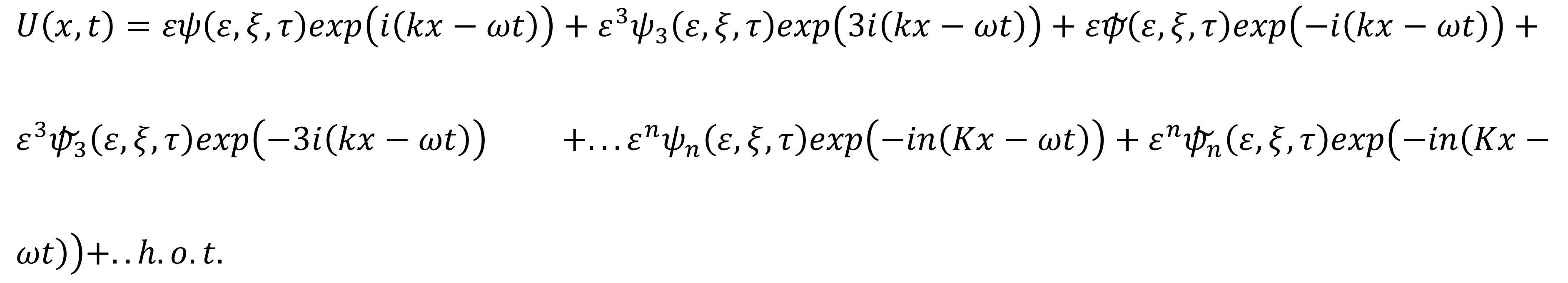
where the wide tilde stands for complex conjugate, n is a positive odds integer and h.o.t. for higher order terms.

Proposition 2.1. 

We assume that in the Fourier expansion (2.8) the following limit exists and is finite

$$\underset{\epsilon \to 0}{\mathit{lim}}{\psi }_n\left(\epsilon ,\xi ,\tau \right)={\psi }_n\left(\xi ,\tau \right)$$

(2.9)

Theorem 2.1. 

The variable change (2.6-2.7) and the Fourier expansion (2.8) imply that

$${\partial }_x\to \gamma {\partial }_{\xi }-\beta \gamma {\partial }_{\tau }+ink$$

(2.10)

$${\partial }_t\to \gamma {\partial }_{\tau }-\beta \gamma {\partial }_{\xi }-in\omega$$

(2.11)

Proof. 

This theorem follows from the observation that

$${\partial }_x\psi \left(\xi ,\tau \right)exp\left(i\left(Kx-\omega t\right)\right)\to ink\psi \left(\xi ,\tau \right)+\left(\epsilon \gamma {\partial }_{\xi }\psi \left(\xi ,\tau \right)-\epsilon \beta \gamma {\partial }_{\tau }\psi \left(\xi ,\tau \right)\right)exp\left(in\left(kx-\omega t\right)\right)$$

(2.12)

$${\partial }_t\psi \left(\xi ,\tau \right)exp\left(i\left(Kx-\omega t\right)\right)\to -in\omega \psi \left(\xi ,\tau \right)+\left(\epsilon \gamma {\partial }_{\tau }\psi \left(\xi ,\tau \right)-\epsilon \beta \gamma {\partial }_{\xi }\psi \left(\xi ,\tau \right)\right)exp\left(in\left(kX-\omega t\right)\right)$$

(2.13)

We now insert the Fourier expansion (2.8) into the Equation (2.2) and consider the equations for each given Fourier mode and to the same $\epsilon$ magnitude.

For $\epsilon$=0, we get the dispersion law for the linear part

$$\left(K^2+2\lambda +1\right)\varphi =0$$

at the next order ${\epsilon }^2$we obtain, for n=1, (NL=nonlinear part),

$$-2iK\left(\gamma {\psi }_{\xi }-\beta \gamma {\psi }_{\tau }\right)-2i\omega \left(\gamma {\psi }_{\tau }-\beta \gamma {\psi }_{\xi }\right)+NL=0$$

(2.14)

and if we choose

$$\beta =\frac{K}{\omega }=V_G$$

(2.15)

we can eliminate the two terms with the $\xi$ derivative.

At last if we consider even the nonlinear terms, the Equation (2.2) yields

$$+2i\gamma \left(K\beta -\omega \right){\psi }_{\tau }-N{\left|\psi \right|}^2\psi =0$$

(2.16)

where

$$N=\frac{4}{3}\lambda +\frac{1}{6}$$

(2.17)

Now we use the polar substitution

$$\psi \left(\xi ,\tau \right)=\rho \left(\xi ,\tau \right)exp\left(i\theta \left(\xi ,\tau \right)\right)$$

(2.18)

in order to separate the linear and nonlinear parts and obtain

$${\rho }_{\tau }=0$$

(2.19)

$$2\gamma \left(K\beta -\omega \right){\theta }_{\tau }-N{\rho }^2=0$$

(2.20)

and then

$$\rho =\rho \left(\xi \right)$$

(2.21)

arbitrary function of the independent variable, but time-constant and

$${\theta }_{\tau }=\frac{\left(8\lambda +1\right)}{12\gamma \left(1+2\lambda \right)}{\rho }^2\left(\xi \right)=\Omega \left(\xi \right)$$

(2.22)

Theorem 2.2. 

There is a phase-locked solution for $\lambda =-\left(\frac{1}{8}\right)$ when the solution frequency is equal to the linear case.

Proof. 

Just look at the Equation (2.22). Phase-locked solutions are observed in many complex systems, nowadays it is a new exciting research field and we give here just two recent examples. It is well known that millimeter-wave (mm-wave) frequencies are required to support the increasing number of connected devices expected from the fifth generation (5G) of mobile communications. As a consequence, radio-frequency (RF) carriers ranging from 10 GHz to 300 GHz and their transport through optical distribution network (ODN) is a very important feature of the future 5G communications. We need optically assisted RF carrier generation to tackle this issue, with a wide use of analog radio-over-fiber (ARoF) architectures. The most important drawback of these optical well known methods is related to the finite coherence of lasers sources, it can dramatically degrades data transmission in analog formats. The use of orthogonal frequency-division multiplexing (OFDM) as the 5G standard allows employing efficient phase noise compensation algorithms. We can find an experimental demonstration of a mm-wave generation technique based on an optical phase-locked loop (OPLL) that fulfills the frequency specifications for 5G [13]. These results support the use of OPLLs as a viable solution to generate mm-wave carriers for 5G and beyond.

Now we consider another important topic connected to phase-locked solutions.

It is well known that there are coherent and incoherent types of random lasers, with broadband and randomly distributed narrow-band lasing spectrum, respectively. No fixed phase relationship has ever been observed between the lasing modes in such lasers. However, experimental observations show a new form of random lasers in patterned organic–inorganic hybrid perovskite MAPbBr_3. Multiple simultaneously lasing modes are stably locked in phase so that lasing lines are achieved with equal spectral separations. In the paper we find the first observation of phase locking between random lasers. It can be performed by the cascaded molecular absorption-emission or cascaded excitation-injection processes between random laser modes.

Theorem 2.3 

Wobbling nonlinear solutions can be observed because of the phase $\Omega \left(\xi \right)$ depending on the solution amplitude and its position.

Proof. 

Theorem 2.3 is the most important result of this paper, i.e., an asymptotic perturbation method is able to find a wobbling behavior in the nonlinear solutions of Equation (2.1). Suitable choices for the arbitrary function$\rho \left(\xi \right)$, based on the Weierstrass function and symmetry reflections, can lead to wobbling solitons.

If we look at the Equation (2.16), we can find that the solutions phase depends on the amplitude $\rho$ and on the $\xi$-variable, so that fractal solutions are connected to the spatial environment.

Wobbling solutions are well known. For example in a recent paper [15], the scattering between a wobbling kink and a wobbling anti-kink in the standard ϕ⁴ model is numerically investigated. A careful study performs the dependence of the final velocities, wobbling amplitudes and frequencies of the scattered kinks on the collision velocity and on the initial wobbling amplitude. The fractal structure becomes more intricate due to the emergence of new resonance windows and the splitting of those arising in the non excited kink scattering [15].

The approximate solution is at order $\epsilon$

$$U\left(x,t\right)=2\epsilon \rho \left(\xi \right)cos\left(kx-\omega t+\Omega \left(\xi \right)t\right)+O\left({\epsilon }^3\right)$$

(2.23)

where $\xi$ is given by (2.6).

Theorem 2.4. 

The validity of the approximate solution (2.23) should be expected to be restricted on bounded intervals of the τ-variable and on time-scale $t=O\left(\frac{1}{{\epsilon }^2}\right)$, otherwise if we want to find solutions on intervals such that $\tau =O\left(\frac{1}{\epsilon }\right)$, then the approximate solution (2.23) loses its validity.

Proof. 

The former statement follows easily from Equations (2.6) and (2.7).

In the Section 3 and Section 4 we will study coherent, phase-locked, envelope wobbling solitary waves and fractal solutions for the nonlinear Equation (2.2).

3. Coherent Solutions

There are many coherent solutions for the nonlinear Equation (2.2).

A solitary wave is possible with the choice

$$\gamma =1.3,\beta =0.8\rho \left(\xi \right)=\frac{A}{cosh\left(B\xi \right)}\mathrm{A}=0.1,\mathrm{B}=2\lambda =1$$

(3.1)

in such a way to obtain an envelope solitary wave given by the Equation (2.23).

$$U\left(x,t\right)=\frac{0.1}{cosh\left(\left(2\left(\gamma \left(x-\beta t\right)\right)\right)\right)}cos\left(0.8\left(\gamma \left(x-\beta t\right)-\left(3+{\Omega }^2\right)\right)\gamma \left(t-\beta x\right)\right)$$

(3.2)

where $\Omega$ is given by (2.23).

Figure 1. Envelope solitary wave with $\gamma =1.3,\beta =0.8$, A=0.1, B=2, $\lambda$=1.

Figure 1. Envelope solitary wave with $\gamma =1.3,\beta =0.8$, A=0.1, B=2, $\lambda$=1.

This solution amplitude propagates with velocity $\beta$=0.8 and the relative modulation is given by the phase velocity V _F=1 that is the light speed. It is obvious that this behavior is connected to the Lorentz-invariant feature of the double sine-Gordon equation.

Theorem 3.1. 

The nonlinear solution phase depends on the solution position, a very important feature for the double sine-Gordon equation.

Proof. 

The above statement follows easily from the Equation (2.22).

Now we study the lump phase-locked solution ($\lambda =-\left(\frac{1}{8}\right)$), with the choice

$$\rho \left(\xi \right)=\frac{A}{B+C{\xi }^2}$$

(3.3)

Figure 2. The nonlinear approximate solution (2.23) for the phase-locked solution with $\gamma =1.3,\beta =0.8$,A=0.1, B=1, C=0.2 $\lambda$=-1/8.

Figure 2. The nonlinear approximate solution (2.23) for the phase-locked solution with $\gamma =1.3,\beta =0.8$,A=0.1, B=1, C=0.2 $\lambda$=-1/8.

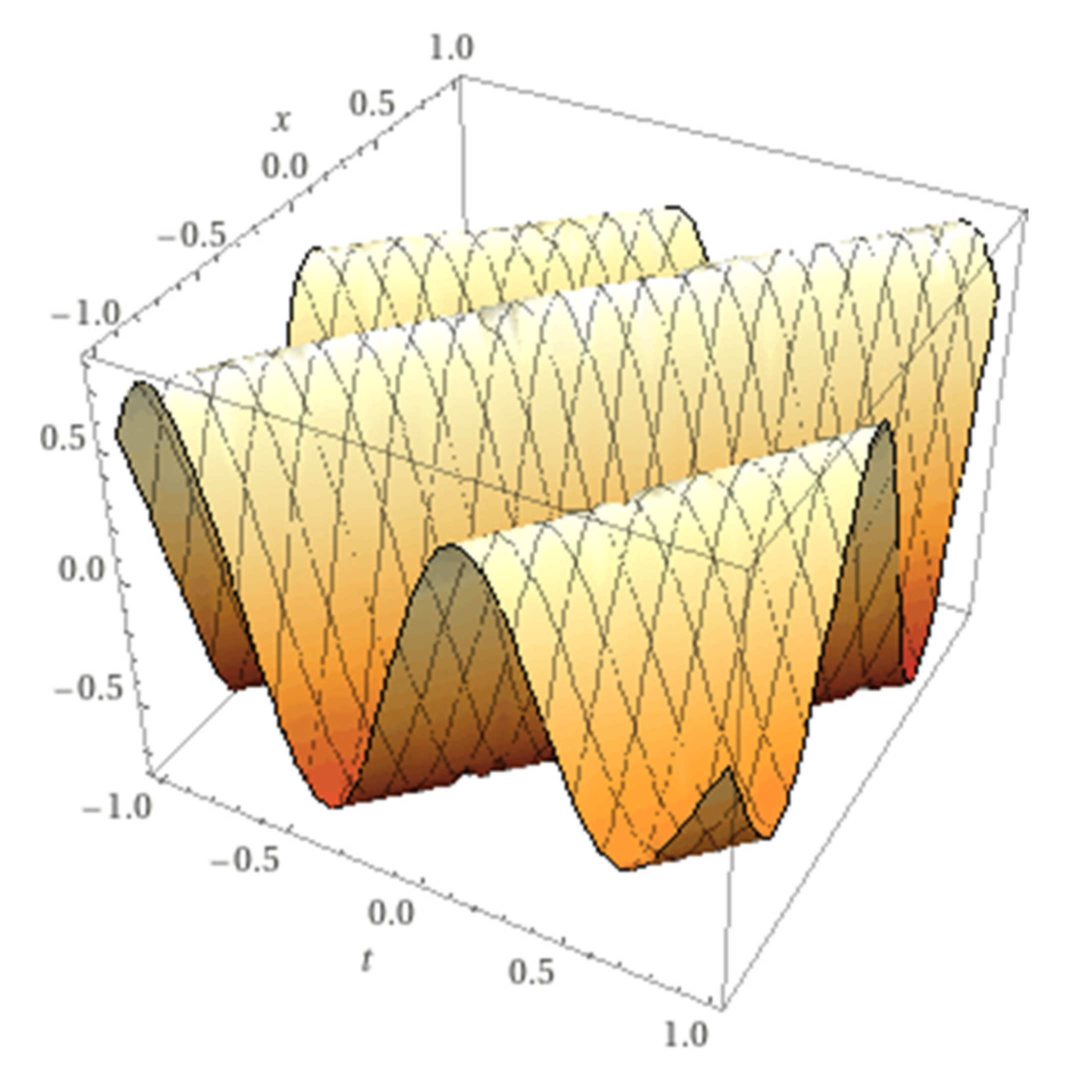
Another coherent solution (2.23) is possible with the choice

$$\rho \left(\xi \right)={Ae}^{\left(B\left|\left(\xi \right)\right|\right)}$$

(3.4)

and it is shown in Figure 3.

4. Fractal Solutions

In this Section we show that even fractal solutions are possible for the nonlinear Equation (2.1). The most important feature is the arbitrary function (2.15) that allow us to obtain chaotic and fractal solutions.

We can consider the stochastic, fractal Weierstrass function W(x). This function is continuous but nowhere differentiable

$$W\left(x\right)={\sum }_{\mathrm{k}=1}^N{\left(c_1\right)}^k\sin \left[{\left(c_2\right)}^{k}x\right]N\to \infty ,$$

(4.1)

with c₂ odd and

$$c_1{c}_2>1+\frac{3\pi }{2}$$

(4.2)

It is well known that the Weierstrass function (1872) was considered at the beginning a pathological function, but Weierstrass faced the most important challenge, disproving the notion that every continuous function is differentiable except on a set of isolated points. Weierstrass demonstrated that continuity did not imply almost-everywhere differentiability. It was a great breakthrough for mathematics, overturning several proofs that relied on geometric intuition and vague definitions of smoothness.

Other famous mathematicians rejected this type of functions and Henri Poincarè called it a “monster” and Weierstrass function was considered "an outrage against common sense". Charles Hermite wrote that this function was a "lamentable scourge". Obviously the function was impossible to visualize until the arrival of computers in the next century, and the results did not gain wide acceptance until practical applications such as models of Brownian motion necessitated infinitely jagged functions (nowadays known as fractal curves). The Mandelbrot pioneering work changed all our beliefs about these fractal functions [16].

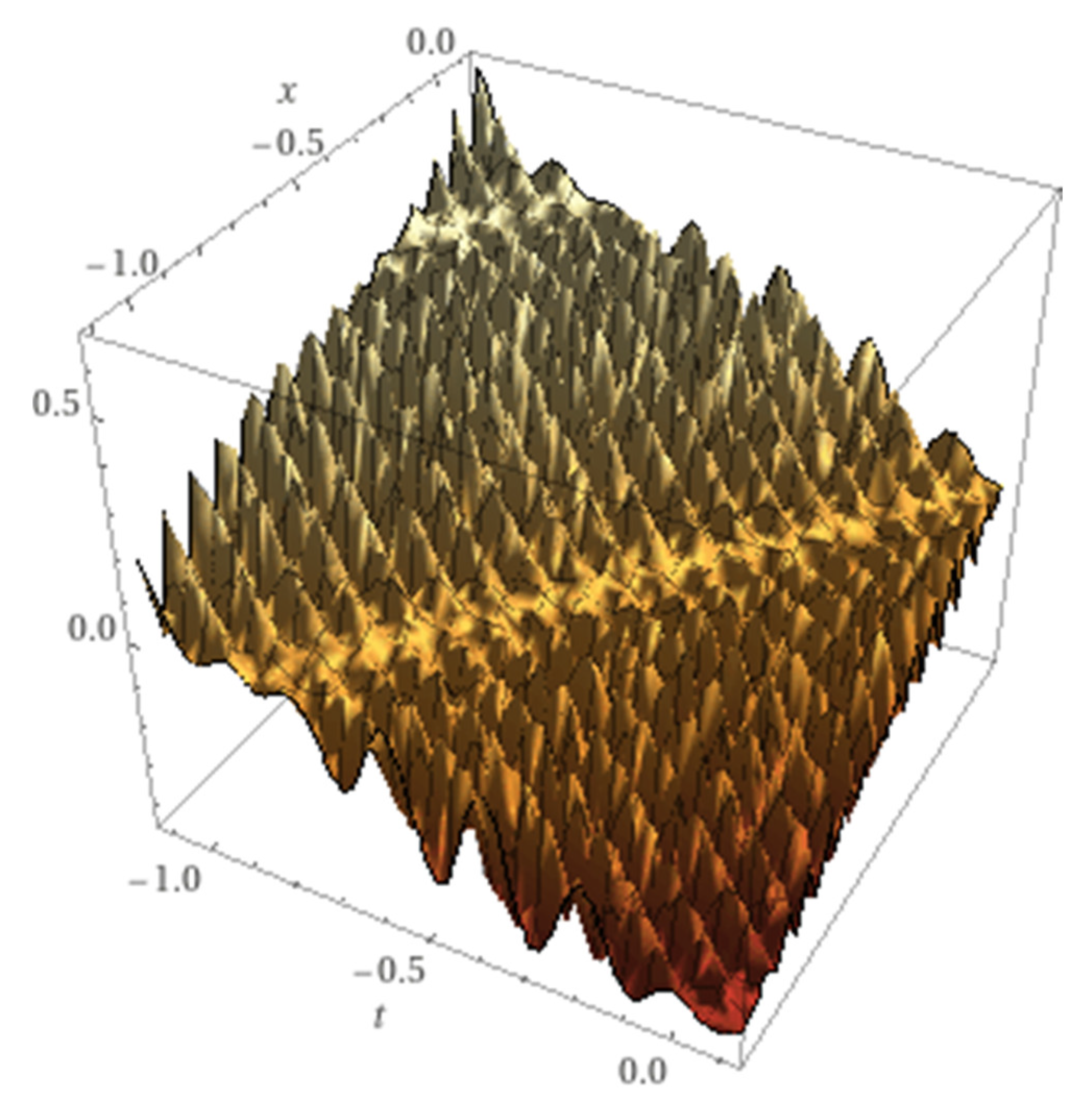
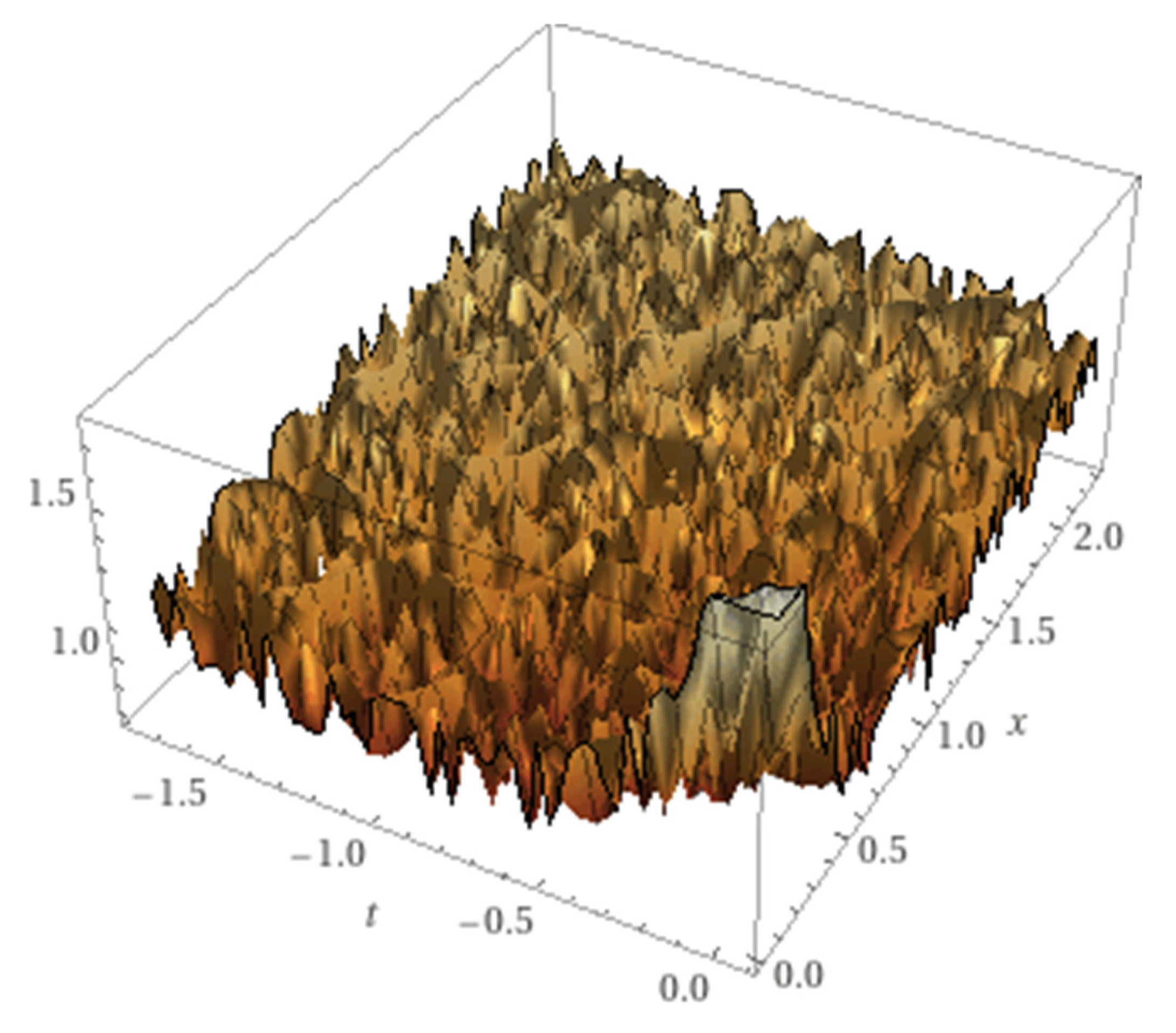
We show in Figure 5, the stochastic fractal lump solution, for simplicity we consider N=5 and calculate the approximate solution (2.23). We find a new type of solutions, the wobbling fractals.

$$\varphi \left(x,t\right)=W\left(\xi \right)cos\left(K\gamma \left(x-\beta t\right)-\left(\omega +\Omega \right)\gamma \left(t-\beta x\right)\right)\frac{A}{B+C{\xi }^2}$$

(4.3)

where $\xi$ is given by (2.6) and $\Omega \left(\xi \right)$by (2.16)

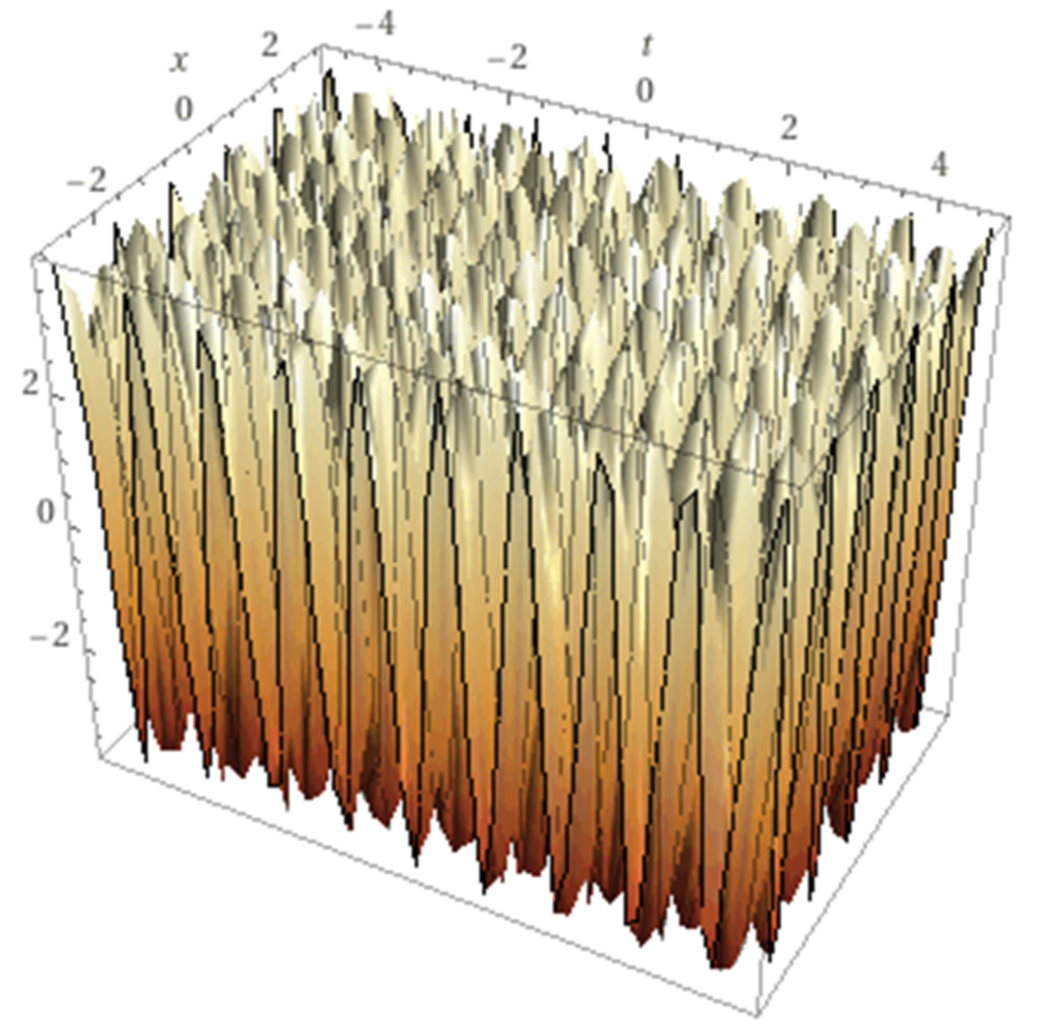
Figure 4. The stochastic fractal solution (4.3). with $\gamma =1.3,\beta =0.8$, A=0.1, B=0.2, C==0.2 $\lambda$=1, c₁=0.4, c₂=20.

Figure 4. The stochastic fractal solution (4.3). with $\gamma =1.3,\beta =0.8$, A=0.1, B=0.2, C==0.2 $\lambda$=1, c₁=0.4, c₂=20.

Note the wobbling behavior, that is the fractal behavior depends on the phase solution and the position.

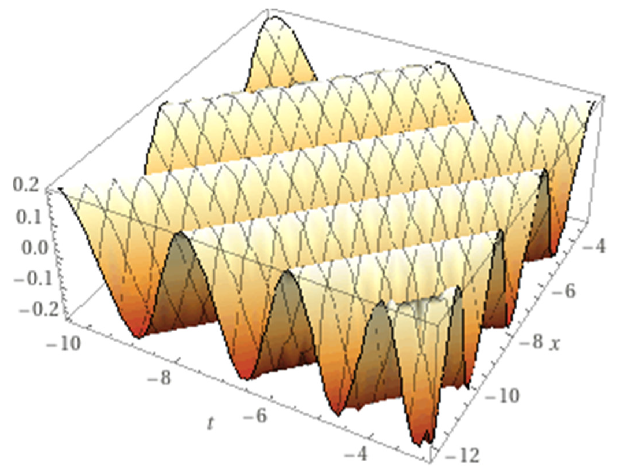
A fractal lump solution is algebraically localized in large scale and possesses self-similar structure near the center of the lump. We consider for example an amplitude fractal dromion

$$\rho \left(\xi \right)=Rexp\left(-C\left(\left|\gamma \left(x-\beta t\right)\right|\right)\right),$$

(4.4)

and R is given by

$$R=2+\sin \left(ln\left(T^2\right)\right)$$

(4.5)

where T is

$$T=W\left(\xi \right)=W\left(\gamma \left(x-\beta t\right)\right)$$

(4.6)

Figure 5. The nonlinear approximate solution (3.1), with $\gamma =1.3,\beta =0.8$, C=0.1, $\lambda$=1, c₁=0.4, c₂=20.

Figure 5. The nonlinear approximate solution (3.1), with $\gamma =1.3,\beta =0.8$, C=0.1, $\lambda$=1, c₁=0.4, c₂=20.

5. Conclusions

We applied the AP method to the DSG Equation (2.1), considering a Lorentz-invariant change of variables with slow time and large space scale. We introduce a parameter $\lambda$ in such a way that, for $\lambda$=0, we obtain the standard sine-Gordon nonlinear equation.

Considering the phase modulation we demonstrated the existence of wobbling nonlinear solutions with the phase depending on the solution amplitude and position.

Moreover for $\lambda$=-1/8, we obtain a phase-locked solution and show its behavior. Nonlinear partial differential equations with phase-locked solutions can be of applicative relevance [13,14,17].

The AP method is then able to obtain wobbling fractal solutions, using also symmetry considerations, and future work can be devoted to find wobbling fractal solutions for other nonintegrable nonlinear equations.

References

- Salamo, G.J.; Gibbs, H.M.; Churchill, G.C. Phys. Rev. Lett. 1974, 33, 273–277. [CrossRef]
- Kr’uchkov, S.V.; Shapovalov, A.I. Sov. Opt. Spectrosc. 1998, 2, 286–291.
- Bullough, R.K.; Caudrey, P.J.; Gibbs, H.M. The Double Sine-Gordon Equations: a physically applicable system of equations. In Solitons, lectures on Current Physics; Bullough, R.K., Caudrey, P.J., Eds.; Springer: New York, 2011; pp. 107–141. [Google Scholar]
- Ablowitz, M.J.; Kruskal, M.D.; Ladik, J.F. SIAM, J. Appl. Math. 1979, 36, 428–434. [CrossRef]
- Bullough, R.K.; Caudrey, P.J. Rocky Mountain J. Math. 1978, 8, 53–60. [CrossRef]
- Olsen, O.H.; Samuelsen, M.R. Wave Motion 1982, 4, 29–35. [CrossRef]
- Mason, A.L. Nonlinear Equations in Physics and Mathematics; Barut, A.O., Ed.; Reidel Publishing Company: Dordrecht, Holland, 1978; pp. 205–218. [Google Scholar]
- Mussardo, G.; Riva, V.; Sotkov, G. Nucl. Phys. B 2004, 687, 189–219. [CrossRef]
- Goldstone, J.; Jackiw, R. Phys. Rev. D 1975, 11.
- Maccari, A. Rogue Waves Generator and Chaotic and Fractal Behavior for the Maccari System with a Resonant Parametric Excitation. Symmetry 2022, 14, 2321–2329. [Google Scholar] [CrossRef]
- Maccari, A. Parametric Resonance for the Hirota-Maccari Equation. Symmetry 2022, 14, 1444–1451. [Google Scholar] [CrossRef]
- Maccari, A. A Reverse infinite period bifurcation for the nonlinear Schrodinger equation in 2+1 dimensions with a parametric excitation. J. Found. Appl. Phys. 2021, 8, 69–76. [Google Scholar]
- Dodane, J.; PérezSantacruz, J.; Bourderionnet, S.; Rommel, G.; Feugnet, A.; Jurado-Navas, L.; Vivien, I. ; Tafur Monroy, Optical phase-locked loop phase noise in 5G mm-wave OFDM ARoF systems. Opt. Commun. 2023, 526, 128872–128876. [Google Scholar] [CrossRef]
- Zhang, X.; Fu, J.H.Y.; Guo, J.; Zhang, Y.; Song, X. Phase-Locking of Random Lasers by Cascaded Ultrafast Molecular Excitation Dynamics. Laser Photonics Rev. 2023. [Google Scholar] [CrossRef]
- Izquierdo, A.A.; Queiroga-Nunes, J.; Nieto, M. Scattering between wobbling kinks. Phys. Rev. D 103, 045003–045006. [CrossRef]
- Mandelbrot, B. Fractals and Chaos; Springer and Verlag: Berlin, 2004. [Google Scholar]
- Grauer, R.; Kivshar, Y.S. Chaotic and phase-locked breather dynamics in the damped and parametrically driven sine-Gordon equation. Phys. Rev. E 1993, 48, 4791–4795. [Google Scholar] [CrossRef]
Figure 3.
The nonlinear approximate solution (3.1), with .
Disclaimer/Publisher’s Note: The statements, opinions and data contained in all publications are solely those of the individual author(s) and contributor(s) and not of MDPI and/or the editor(s). MDPI and/or the editor(s) disclaim responsibility for any injury to people or property resulting from any ideas, methods, instructions or products referred to in the content. |
© 2023 by the authors. Licensee MDPI, Basel, Switzerland. This article is an open access article distributed under the terms and conditions of the Creative Commons Attribution (CC BY) license (http://creativecommons.org/licenses/by/4.0/).
Copyright: This open access article is published under a Creative Commons CC BY 4.0 license, which permit the free download, distribution, and reuse, provided that the author and preprint are cited in any reuse.