Submitted:
06 February 2023
Posted:
06 February 2023
Read the latest preprint version here
Abstract
Multivariate predictive analysis of the Stream-Water (SW) parameters (discharge, water level, temperature, dissolved oxygen, pH, turbidity, and specific conductance) is a pivotal task in the field of water resource management during the era of rapid climate change. The highly dynamic and evolving nature of the meteorological and climatic features have a significant impact on the temporal distribution of the SW variables in recent days making the SW variables forecasting even more complicated for diversified water-related issues. To predict the SW variables, various physics-based numerical models are used using numerous hydrologic parameters. Extensive lab-based investigation and calibration are required to reduce the uncertainty involved in those parameters. However, in the age of data-informed analysis and prediction, several deep learning algorithms showed satisfactory performance in dealing with sequential data. In this research, a comprehensive Explorative Data Analysis (EDA) and feature engineering were performed to prepare the dataset to obtain the best performance of the predictive model. Long Short-Term Memory (LSTM) neural network regression model is trained using over several years of daily data to predict the SW variables up to one week ahead of time (lead time) with satisfactory performance. The performance of the proposed model is found highly adequate through the comparison of the predicted data with the observed data, visualization of the distribution of the errors, and a set of error matrices. Higher performance is achieved through the increase in the number of epochs and hyperparameter tuning. This model can be transferred to other locations with proper feature engineering and optimization to perform univariate predictive analysis and potentially be used to perform real-time SW variables prediction.
Keywords:
Deep neural network
; long short-term memory
; water quality
; discharge
; stream-water
1. Introduction
With the ever-increasing demand, surface water has become the most crucial resource among the communities [1,2,3,4]. From the scale of industrial and electricity generation to the scale of agricultural and drinking purposes, the availability of surface water needs to be abundant with the appropriate quantity and quality [5,6,7]. Among all the surface water bodies, Stream-Water (SW) is considered the most important source to provide countless benefits to human beings [8,9,10]. Conveying not only the drinking water to the communities and irrigation water for agricultural purposes, but streams can also significantly wash away the wastes, and provide habitat for wildlife and hydroelectricity. Often, it is used for several recreational purposes e.g., fishing, swimming, and boating [11,12]. The selected SW quantity variables are discharge and water level of the stream is highly influential on the overbank flooding in the surrounding area, demand of water supply, and fluvial ecology. Aquatic life is impacted significantly due to the temporal dynamics between the seasons of the stream discharge and water level [13,14,15,16,17]. Surface water quality standards are established by examining surface water quality measures such as dissolved oxygen, pH, turbidity, toxic substances, and aquatic macroinvertebrate life [18,19]. According to the New Jersey Department of Environmental Protection (NJDEP) (2012), Integrated Water Quality Report, at least one designated use is classified as Not Supporting (NS) in every sub watershed in Trenton [20]. Selected SW quality parameters in this study are temperature, Dissolved Oxygen (DO), pH, turbidity and Specific Conductance (SC). The temperature being the most important ecological factor is directly correlated to the physical, chemical, and biological properties of water [21,22,23,24]. DO is essential for aquatic life to survive, with differing oxygen concentration tolerances among species and life stages [25]. The pH and SC have a substantial impact on the other metrics of overall water quality, both constructively and adversely. According to the previous studies, the positive correlation between them and nitrate ions, ammonia, phosphorus, calcium, and magnesium, or even the detrimental influence of high pH on exotic species invasions, could induce disruptions in natural ecosystems [26,27,28]. Turbidity is the measure of relative clarity of water caused by suspended particles or dissolved whereas high values can significantly reduce the aesthetic quality of streams and influence natural migrations of species [29]. Assessment of turbidity improves the evaluation and indication of fecal contamination in water bodies such as Escherichia coli, the most common water infection [30,31].
Traditional physics-based numerical models (e.g., HEC-RAS, MIKE) involve spatial and temporal discretization for the entire computational space to compute SW variables which require high computational efforts [32,33]. Various numerical scheme (e.g., Finite Volume, Finite Element, Finite Difference) is used to solve partial differential equations i.e., Navier-Stokes equation coupled with the conservation of mass equation. The cost of spatial and temporal discretization increases exponentially with the increase in the required resolution and accuracy [34,35,36]. Input data for the physics-based river models consist of a significant amount of morphological, operational, and measured data. Data preprocessing for the physic-based models can be daunting depending on the spatial and temporal tags of the target variables. Physics-based numerical models require measurable and empirical parameters to estimate the target variables. A substantial amount of work to retrieve the parameters and constants through extensive laboratory-based experimentation and calibration is also a prerequisite which make these models computationally costly for practical implication with varying scale [37].
Data-informed predictive models provide an efficient alternative approach to forecast and monitor both the SW flow and quality parameters where only observed data can be used for the prediction instead of using many environmental factors required by the physics-based models. They offer reduced computational effort while simplifying complicated system and predict the outcomes using the observational only without any physics-based equations [38,39,40,41]. In recent days, Deep Learning (DL), an advanced sub-field of artificial intelligence, has become a popular choice in predictive modelling in the field of water resource management [42,43]. However, the traditional deep neural network algorithms (e.g., Multilayer Perceptron (MLP) do not have the ability to learn sequential data because they cannot store previous information, resulting in a constrained prediction capability for long-term time series, e.g., temporal distribution of the water table depth [44,45]. The MLP algorithms needs complex procedures in the data pre-processing stage to obtain good performance in predicting the target variables [46,47,48]. While the comprehensive data pre-processing can bolster the ability of a MLP model to learn the observed data, subjective user intervention is still necessary, e.g., selecting the number of reconstructed components [49]. In addition, the pre-processing require substantial amount of time as many reconstructed components needs to be calculated [50].
The Long Short-Term Memory (LSTM) is a special type of neural network which stores extended sequential data in the hidden memory cell for further processing [51,52]. LSTM performs well in processing long term sequential data, utilizing its sophisticated network structure specifically designed to carry the temporal linkage of the time series data. Water quality and quantity data have not been widely investigated in previous work employing LSTM. Therefore, compared with aforementioned MLP model, the proposed LSTM model only requires a simple data pre-processing method [53]. LSTM neural network is recurrent in nature, where the connections between units form a directed cycle allowing data to flow both forwards and backwards within the network. Therefore, the model is capable of preserving the past information and use them further for future prediction. LSTM model have already been used as a very advanced model in the field of DL, e.g., speech recognition, natural language processing, automatic image captioning and machine translation [44,54,55]. However, only a few studies have applied Recurrent Neural Networks (RNNs) or LSTMs to forecast multivariate time series data in the field of water resource [56,57,58]. The objective of this research is to untangle the pattern of the temporal distribution and linkage among the aforementioned SW variables and perform predictive analysis on the using the previous observed data. To accomplish the goal, a comprehensive Exploratory Data Analysis (EDA) is conducted to investigate the temporal dynamics of the SW variables and LSTM prediction is performed to predict the future values based on past records. Following sections of the paper demonstrate the study location, data source and collection, EDA, LSTM prediction, performance evaluation and possible future directions.
2. Data and Methods
2.1. Study Location and Workflow
The monitoring station used in this research is located along the Central Delaware River, in Trenton City, Mercer County, NJ [59]. It's positioned 450 feet upstream from Trenton's Calhoun Street Bridge, 0.5 miles upstream from Assunpink Creek, 0.9 miles north of Morrisville, PA. The Hydrologic Unit number for this station is 02040105 based on the USGS water resources and it is located at 40°13'18" N, 74°46'41" W coordinates referenced to the North American Datum of 1983 with the 6,780 mi² of drainage area (Figure 1).
Entire workflow of the EDA and LSTM prediction tasks are divided into three distinction stages. In the first step, data collection from the USGS web portal, an exploratory analysis of the SW variables and feature engineering to transform the data for training/testing the LSTM algorithm is conducted. Variables used in the analysis are listed in the Table 1. Activities in the first step are categorized as the transformer. After investigating the dataset and performing data transformation on the variables, LSTM neural network is trained using the data prepared in the first step to perform predictive analysis. LSTM neural networks regression model is assessed using several error matrices. These activities are categorized as estimator. The LSTM algorithm is tuned and optimized by altering the hyperparameters to reduce the errors in the prediction and achieve satisfactory performance. The third step namely evaluator, the model is deployed to predict the recession rate for a new set of target variables. Model performance is further improved through iterative incorporation and validation of the input variables.
The LSTM workflow of predicting the SW performance indicator is illustrated in the Figure 2. In the first step of the workflow in he time series of the SW variables are retrieved from the USGS National Water Information System: Web Interface [59]. The range of the time series data for all the variables was different due to the various recorded duration. Mean values of the SW variables are used in this study. The range of the data used in this research is from 02/25/2006 to 03/08/2022 with observed data of seven years. Historically, for the years 1898 to 1906, peak discharges were measured at Lambertville, NJ, 14.3 miles upstream of the Calhoun Street bridge. The maximum discharge was recorded on 8/20/1955 with the amount of 329,000 ft³/s and the minimum discharge was 1,180 ft³/s, on 10/31/1963. Extreme flooding occurred on 10/11/1903 when the water level reached an elevation of 28.5 ft above NGVD of 1929 which resulted in a discharge amount of 295,000 ft³/s [59].
2.2. Multivariate Exploratory Data Analysis (EDA)
In the second activity in the Figure 2, a detailed EDA is performed to perceive the attributes and characteristics of the multivariate dataset. EDA is the pivotal step to perform preliminary investigations on data in order to obtain satisfactory performance of the LSTM model. Internal temporal distribution of all the SW variables is explored through multiple visual techniques and numerical indices. EDA consists of process of performing initial investigation of the SW variables to understand the hidden pattern of the distribution of the variables. EDA is further divided into several activities. They are denoted as the descriptive statistics, outliers/extreme values detection, and normality check. Descriptive statistics provides a great approach to delineate the distribution of the values of the SW variables with the number of data points, mean, standard deviation, percentiles, interquartile range, and range. Full multivariate descriptive statistics is shown in the Table 2. To demonstrate the normality in the variables, histograms with density plot is used as a visual representation and Pearson’s Coefficient of Skewness (PCS) is use as a numerical indicator of skewness. Numerical imputation is performed to make the dataset consistent by filling missing values with the Nearest Neighbors (NN) of the datapoints [60].
Water quantity variables e.g., discharge and water level and water quality variable, turbidity show higher non-normality compared to the other SW variables. Numerical measure of non-normality/skewness, PCS values of discharge, water level and turbidity are also higher than the PCS values of other SW variables which indicates relatively less normality.
Figure 3 illustrates the linear connection between two SW variables. Low values of the linear coefficients delineate the overall non-linearity among several variables is high. The direction of the linear relationships is found to be both positive and negative. A few variables are approximately linearly correlated e.g., discharge and water level, temperature and DO, SC, and pH.
2.3. Feature Engineering (FE)
FE is performed after a successful preliminary investigation on the dataset using EDA. Without a successful FE, LSTM method may not yield to a satisfactory performance with minimum error. An adequate optimization through the iterative gradient descent cannot be reached without a successful scrutiny of the dataset. Therefore, a comprehensive feature engineering is carried out to transform the variables most suitable for the learning algorithm of LSTM [61,62]. FE in this research involves imputation, data transformation, data standardization and splitting the dataset into training, testing, and validation sets. Imputation in preformed to fill the null values so that the entire dataset becomes consistent. Null values or observation were found in every series due to sensor malfunctions. These cells in the dataset are imputed with the values of the NN of the blank cell. However, due to the reduction of the size of the dataset as a result of the exclusion of the observations, it is implemented in this study. After a successful imputation with median values of the variables, distribution of the variable series is checked visually and numerically to confirm the normality. PCS is used as an indicator of the normality of the variables. As the distribution of the values of discharge and water level is highly skewed to the left showing a significant non-normally, the neural network regression algorithms without appropriate data transformation does not contribute to satisfactory outcomes with good optimization [63,64,65]. Data transformation is performed to decrease the non-normality of discharge and water level. In this research, logarithmic transformation is implemented to transform the distribution of the features more to the normal distribution to reach the maximum performance of the LSTM model. In the Figure 4 distributions of the transformed and observed discharge and water level series can be seen. PCS values increases for all the transformed series compared to the observed series showing the increase in the normality.
The LSTM recurrent neural network model uses the gradient descent technique where the feature value affects the step size of the technique. Smooth progress towards minima in gradient descent requires the update of the steps at the same rate for all the feature values. To establish the LSTM model's training and testing dataset, all of the values are normalized utilizing Equation 1.
X denotes the variable of interest and subscript norm, max and min represent the normalized variable, maximum and minimum value of the values of the variable. The entire normalized variable series is split into a training set and a testing set that is used to test/evaluate the model.
2.4. Long Short-term Memory (LSTM) Recurrent Neural
LSTM has become a very popular algorithm to deal with time series data in the DL forecasting where variables are dependent on the previous information along the series [67,68]. LSTM can capture the long-term dependencies and linkage among the variables [69]. High computational effort and time is needed by recurrent backpropagation to learn to store long-term information because of the decaying error backflow [70]. Hence, the concept of the vanishing gradient problem in recognizing long-term dependency of RNN was introduced [71]. LSTM feedback connections is the principal component of processing and recalling long-term information and a unique feature which makes it different from the traditional feedforward neural network.
Both long-term memory (c[t-1]) and short-term memory (h[t-1]) are processed in a typical LSTM algorithm through the utilization of multiple gates to filter the information. For an unchanged flow of gradients, forget and update gates update the memory cell state [72,73]. Three gates i.e., input gate ig (pink), forgot gate fg (red) and output gate og (violet) and cell state (green) handle the information flow by writing, deleting, preserving past information, and reading respectively (Figure 5). Hence, LSTM is capable in memorizing information at different lead times making it suitable in time series prediction within a certain interval [74]. In forget gate, long-term information enters and passes through a filtration where unnecessary information is discarded. The forget gate filter out unnecessary data by using the sigmoid activation function where the range of the function is 0 and 1 for open and close status, respectively. Input gate filter and quantify the significance of a new data coming as input to the cell. Like the forget fate, input gate filters out information by using binary activation functions and controls the flow of both long-term and short-term information. The output gates regulate the value of the upcoming hidden state which is a function of the information on previous inputs.
In this research, a neural network with one LSTM hidden unit accompanied by a dense layer connecting the LSTM target output at the last time-step (t-1) to a single output neuron with non-linear activation function. The LSTM model was trained using the DL library, Keras in Python, the ReLU activation function, and the coefficient of determination (), and Nash Sutcliffe model efficiency coefficient (E) loss function. To predict the SW variable of a time-step in future e.g., daily/weekly, values of the variables at previous time-steps are used. Hyperparameters are tuned to maximize the performance of the LSTM model through iterative trial and error approach. In this study, Keras, python library which offers a space search for machine learning algorithms is used to find the best combination of the hyperparameters [75,76]. Hyperparameter of the LSTM algorithm considered in this study are the size of epoch and batch and number of neurons.
2.5. Model Evaluation and improvement
In the model evaluation step in the fifth activity in Figure 2, the performance of the LSTM model is evaluated using top three standard error matrices e.g., , and the E. Error matrices provide numeric values as the model performance indicator by comparing the observed and predicted values. The value is used to evaluate the LSTM model in showing the model performance improvement. The highest score corresponds to the best predictive accuracy. In addition to the and E are used to illustrate the model response due to the variation in the lead time. The better the model fits the data, the closer the value is to 1. The third evaluation metric refers to the E and is one of the most widely used metrics for evaluating a hydrologic model's performance. can be classified as one of the scaled forecasts that compare the predicted error to the observed error [77,78]. Having a positive value for E, shows that the prediction and computed recession rate value is better than simply selecting the average observed value. In order to ensure that training is effectively fit, it is vital to choose a model's hyperparameters and consider carefully the controlling parameters that impact the learning rate of the model. By optimizing the size of the epoch, batch, and neurons in the stochastic process of the LSTM neural network, the LSTM algorithm's performance in predicting SW parameters is further improved.
3. Results and Discussion
LSTM neural network are used to predict the multivariate SW variables based on the previous time series data. Several lead time durations e.g., 6 hours, 12, hours, 1 day, 3 days, 1 week, 2 weeks, 3 weeks and 1 month are used to forecast the future values of variables simultaneously. Predicted values are compared to the observed dataset to quantify the error matrices. , and E are used to estimate the error from the predicted SW variables. Model performance is improved by increase in the number of epochs. Error matrices are obtained through multiple models runs to demonstrate the linkage between the model performance and the lead times. Hyperparameters of the LSTM model are adjusted to optimize the model performance considering a set of batch size, epoch size and total number of neurons.
3.1. Predicted and Observed SW variables
Th output from the LSTM algorithm is compared to the observed values of the SW variables through visual representation in the Figure 6. Both the observed and predicted values of the SW variables are plotted for the entire time series against the number of observations. The overall distribution of the predicted values of SW variables is approximately identical to the observed data providing a satisfactory performance of the LSTM algorithm. The error metrices recorded for all variables and full time series shows LSTM performed well in case of both train/test set. After the LSTM model is trained, the entire observed dataset is divided into training and testing sets with the proportion of 80% and 20%. Training dataset is used to train the model and testing dataset is used to evaluate the model performance. In the Figure 6, orange portion of the plot illustrate training portion of the dataset whereas the green portion shows the testing portion. Dashed lines with blue color show the observed data.
3.1. Model Evaluation Matrices and Improvement
The performance of the LSTM neural network is evaluated using three error matrices e.g., Root Mean Square Error (RMSE), the and E. The performance of the model also evaluated and improved through increasing the number of iterations i.e., epoch in the neural network. The value of error matrices is observed with the increase in the number of epochs in the Figure 7. The model performance increases significantly from the very beginning of the iteration for both the train and test scenarios. The trend of change in the increase in the values reach a near-steady state after 20 epochs. Local decease in the performance i.e., increase in the RMSE value can be seen after 20 epochs. Further The performance variation with the change in the lead time regarding RMSE is represented in the Figure 7.
Error matrices e.g., and E are documented for several lead times. Lead times are pivotal parameters of LSTM algorithm towards model performance. Lead time values are 1 day, 2 days, 3 days, 4 days, 5 days, 6 days and one week. The values of and E decreases with the increase in lead time, showing the degradation in the model performance with increase in the lead times (Figure 8). Therefore, selection of the lead times should be based on the model performance and necessity.
Accuracies in the LSTM prediction for all SW parameters are presented in the Figure 9 with the help of coefficient of determination, . Observed and predicted values of SW variables from the LSTM prediction are plotted to determine the value. The range of the value for all SW parameters 0.552 to 0.953 delineates satisfactory performance from LSTM model prediction overall. The best prediction with minimum error is found for the DO prediction with the value of 0.953.
3.3. Hyperparameters Optimization
To achieve the best possible model configuration for the predictions, hyperparameter optimization of the LSTM algorithm is of utmost importance. The optimized parameters that are only effective for the SW parameters are taken into account in this study because the neural network tuning procedure is stochastic. At first step, the epoch size is optimized keeping the batch of 4 and a single neuron. A set of increasing number of epochs (50, 75, 100, 125 and 150) is chosen to observe the response in LSTM model performance. In the same fashion, a set of batch sizes (1, 3 and 5) and neurons (1-5) are selected with a constant epoch size of 1000 to see the performance improvement. Epoch size of 2000 is selected to further the optimization process with the batch size and the number of neurons as it provides the highest value. A batch size of 1 and 5 neurons provides further highest values which can be seen in the Figure 10. Therefore, an epoch size of 2000, batch size of 3 and number of neurons of 5 is considered as the best hyperparameter combination for LSTM model prediction.
4. Conclusions
Multivariate prediction of the SW variables under both the water quantity and quality categories at a point location using the observed data can be highly beneficial to the water managers and decision makers to perceive the future flooding, irrigation works and fluvial ecology and aquatic life. Unlike the physics-based numerical models where additional terrain, meteorological data and human interventions are pre-requisite, the proposed approach relies only on the previously recorded data of the variables. The LSTM framework to predict the SW variables can be highly beneficial for the nearby community where the short-term prediction of the dynamics of the SW variables daily/weekly/monthly in future play a critical role. In the prediction of water quantity i.e., discharge and water level can substantially aid to prepare for the flood inundation, irrigation work and water supply demand. Prior knowledge of water quality of the SW can be highly beneficial to manage the aquatic life. As the model proposed uses only previous observed data of the variables, additional burden of input data and human intervention is not required for prediction work. Several approaches through physics-based numerical modelling techniques are proven inefficient in terms of real-time forecasting and computational efficiency. On the contrary, the application of the data-informed predictive models is highly efficacious in predicting various SW variables without taking complicated differential equations and assumptions into consideration. LSTM algorithm is capable of preserving both the short- and long-term pattern of the time series to forecast. Traditional physics-based numerical modelling tool requires assumptions, other correlated variables, and expensive calibration of the parameters.
This study contributes to a reproducible template to investigate the uniqueness of the temporal dynamics of SW variables through extensive EDA. Hidden pattern of the distribution of SW variables over seven years of data is discovered various up-to-date data exploration tools which is a mandatory requirement for the satisfactory training of LSTM algorithm. After a successful training step, LSTM is tuned and optimized through an explicit iterative performance record which can further be transferred to forecast SW variables in the identical geographical location. The performance of the LSTM algorithm in predicting the river discharge illustrates the algorithm is highly suitable to the discharge time series. Several error matrices show promising performance with minimum error. The proposed LSTM configuration is proved to offer satisfactory performance for the SW variables with the lead times up to one week. However, increasing the lead time increases the error in prediction limiting the performance of the LSTM model. Physics-based models are also incompetent in real-time prediction where the proposed LSTM can easily be coupled with the sensor and cloud to predict the SW variables in real time. Computational time may increase exponentially with the increase of the size of the dataset. Principle parameters obtained after the training process with minimum error are number of neurons, batch, and epoch size. The parameters optimized to obtain the best the LSTM configuration after training the model can be transferable in the similar climatic and geographic regions. For instance, if the distribution of the values of the SW variables are identical e.g., the difference among the PCS values being negligible, the parameters of trained LSTM model can be transferred and used for predictive analysis in a different location. However, we should not use our LSTM model in an area where the distribution of the features values through time is dissimilar. Future research should be conducted to incorporate high performance computing and cloud-based operations to obtain smart predictive tool to utilize the revolution in data storage capability and computational efficiency. LSTM models with different configurations should also be applied in different geographical and climatic locations to investigate the transferability of the model.
Author Contributions
Conceptualization, S.G.; methodology, S.G. and N.N.; software, N.N.; validation, N.N.; formal analysis, N.N.; investigation, S.G. and N.N.; resources, S.G.; data curation, N.N.; writing—original draft preparation, S.G. and N.N.; writing—review and editing, S.G. and N.N.; visualization, N.N.; All authors have read and agreed to the published version of the manuscript.
Funding
This research did not receive any specific grant.
Data Availability Statement
Data collected for the study can be made available upon request from the corresponding author.
Conflicts of Interest
The authors declare no conflict of interest.
References
- Uddin, Md.G.; Nash, S.; Olbert, A.I. A Review of Water Quality Index Models and Their Use for Assessing Surface Water Quality. Ecol. Indic. 2021, 122, 107218. [Google Scholar] [CrossRef]
- Ni, X.; Parajuli, P.B.; Ouyang, Y.; Dash, P.; Siegert, C. Assessing Land Use Change Impact on Stream Discharge and Stream Water Quality in an Agricultural Watershed. CATENA 2021, 198, 105055. [Google Scholar] [CrossRef]
- Simeonov, V.; Stratis, J.A.; Samara, C.; Zachariadis, G.; Voutsa, D.; Anthemidis, A.; Sofoniou, M.; Kouimtzis, Th. Assessment of the Surface Water Quality in Northern Greece. Water Res. 2003, 37, 4119–4124. [Google Scholar] [CrossRef]
- Wang, R.; Kim, J.-H.; Li, M.-H. Predicting Stream Water Quality under Different Urban Development Pattern Scenarios with an Interpretable Machine Learning Approach. Sci. Total Environ. 2021, 761, 144057. [Google Scholar] [CrossRef] [PubMed]
- Shah, M.I.; Alaloul, W.S.; Alqahtani, A.; Aldrees, A.; Musarat, M.A.; Javed, M.F. Predictive Modeling Approach for Surface Water Quality: Development and Comparison of Machine Learning Models. Sustainability 2021, 13, 7515. [Google Scholar] [CrossRef]
- Li, K.; Wang, L.; Li, Z.; Xie, Y.; Wang, X.; Fang, Q. Exploring the Spatial-Seasonal Dynamics of Water Quality, Submerged Aquatic Plants and Their Influencing Factors in Different Areas of a Lake. Water 2017, 9, 707. [Google Scholar] [CrossRef]
- Li, K.; Wang, L.; Li, Z.; Xie, Y.; Wang, X.; Fang, Q. Exploring the Spatial-Seasonal Dynamics of Water Quality, Submerged Aquatic Plants and Their Influencing Factors in Different Areas of a Lake. Water 2017, 9, 707. [Google Scholar] [CrossRef]
- Hamid, A.; Bhat, S.U.; Jehangir, A. Local Determinants Influencing Stream Water Quality. Appl. Water Sci. 2019, 10, 24. [Google Scholar] [CrossRef]
- Hamid, A.; Bhat, S.U.; Jehangir, A. Local Determinants Influencing Stream Water Quality. Appl. Water Sci. 2019, 10, 24. [Google Scholar] [CrossRef]
- Mehedi, M.A.A.; Reichert, N.; Molkenthin, F. SENSITIVITY ANALYSIS OF HYPORHEIC EXCHANGE TO SMALL SCALE CHANGES IN GRAVEL-SAND FLUMEBED USING A COUPLED GROUNDWATER-SURFACE WATER MODEL. 2020, 10.13140/RG.2.2.19658.39366. [CrossRef]
- Full Article: How Much Is an Urban Stream Worth? Using Land Senses and Economic Assessment of an Urban Stream Restoration. Available online: https://www.tandfonline.com/doi/full/10.1080/13504509.2021.1929546 (accessed on 16 May 2022).
- Society, N.G. Stream. Available online: http://www.nationalgeographic.org/encyclopedia/stream/ (accessed on 16 May 2022).
- Onabule, O.A.; Mitchell, S.B.; Couceiro, F.; Williams, J.B. The Impact of Creek Formation and Land Drainage Runoff on Sediment Cycling in Estuarine Systems. Estuar. Coast. Shelf Sci. 2022, 264, 107698. [Google Scholar] [CrossRef]
- Salimi S, Scholz M. Importance of water level management for peatland outflow water quality in the face of climate change and drought. Environ Sci Pollut Res Int. 2022 Oct;29(50):75455-75470. Epub 2022 Jun 2. PMID: 35653024; PMCID: PMC9553818. [CrossRef]
- Tremblay, J.-É.; Raimbault, P.; Garcia, N.; Lansard, B.; Babin, M.; Gagnon, J. Impact of River Discharge, Upwelling and Vertical Mixing on the Nutrient Loading and Productivity of the Canadian Beaufort Shelf. Biogeosciences 2014, 11, 4853–4868. [Google Scholar] [CrossRef]
- Ji, H.; Pan, S.; Chen, S. Impact of River Discharge on Hydrodynamics and Sedimentary Processes at Yellow River Delta. Mar. Geol. 2020, 425, 106210. [Google Scholar] [CrossRef]
- Mehedi, M.A.A.; Yazdan, M.M.S. Automated Particle Tracing & Sensitivity Analysis for Residence Time in a Saturated Subsurface Media. Liquids 2022, 2, 72–84. [Google Scholar] [CrossRef]
- WHITEHEAD, P.G.; WILBY, R.L.; BATTARBEE, R.W.; KERNAN, M.; WADE, A.J. A Review of the Potential Impacts of Climate Change on Surface Water Quality. Hydrol. Sci. J. 2009, 54, 101–123. [Google Scholar] [CrossRef]
- Alnahit, A.O.; Mishra, A.K.; Khan, A.A. Stream Water Quality Prediction Using Boosted Regression Tree and Random Forest Models. Stoch. Environ. Res. Risk Assess. 2022. [Google Scholar] [CrossRef]
- Yagecic_monitoring_NJWEAmay2018.Pdf.
- Benyahya, L.; Caissie, D.; St-Hilaire, A.; Ouarda, T.B.M.J.; Bobée, B. A Review of Statistical Water Temperature Models. Can. Water Resour. J. Rev. Can. Ressour. Hydr. 2007, 32, 179–192. [Google Scholar] [CrossRef]
- Kelleher, C.A.; Golden, H.E.; Archfield, S.A. Monthly River Temperature Trends across the US Confound Annual Changes. Environ. Res. Lett. 2021, 16, 104006. [Google Scholar] [CrossRef] [PubMed]
- Ducharne, A. Importance of Stream Temperature to Climate Change Impact on Water Quality. Hydrol. Earth Syst. Sci. 2008, 12, 797–810. [Google Scholar] [CrossRef]
- van Vliet, M.T.H.; Ludwig, F.; Zwolsman, J.J.G.; Weedon, G.P.; Kabat, P. Global River Temperatures and Sensitivity to Atmospheric Warming and Changes in River Flow. Water Resour. Res. 2011, 47. [Google Scholar] [CrossRef]
- (2) (PDF) A Review of Dissolved Oxygen Requirements for Key Sensitive Species in the Delaware Estuary Final Report. Available online: https://www.researchgate.net/publication/329070843_A_Review_of_Dissolved_Oxygen_Requirements_for_Key_Sensitive_Species_in_the_Delaware_Estuary_Final_Report (accessed on 22 May 2022).
- Ehrenfeld, J.G.; Schneider, J.P. Chamaecyparis Thyoides Wetlands and Suburbanization: Effects on Hydrology, Water Quality and Plant Community Composition. J. Appl. Ecol. 1991, 28, 467–490. [Google Scholar] [CrossRef]
- Dow, C.L.; Zampella, R.A. Specific Conductance and PH as Indicators of Watershed Disturbance in Streams of the New Jersey Pinelands, USA. Environ. Manage. 2000, 26, 437–445. [Google Scholar] [CrossRef] [PubMed]
- Using-Multiple-Regression-to-Quantify-the-Effect-of-Land-Use-on-Surface-Water-Quality-and-Aquatic-Communities-in-the-New-Jersey-Pinelands.Pdf.
- Money, E.S.; Carter, G.P.; Serre, M.L. Modern Space/Time Geostatistics Using River Distances: Data Integration of Turbidity and E. Coli Measurements to Assess Fecal Contamination Along the Raritan River in New Jersey. Environ. Sci. Technol. 2009, 43, 3736–3742. [Google Scholar] [CrossRef] [PubMed]
- Tousi, E.G.; Duan, J.G.; Gundy, P.M.; Bright, K.R.; Gerba, C.P. Evaluation of E. Coli in Sediment for Assessing Irrigation Water Quality Using Machine Learning. Sci. Total Environ. 2021, 799, 149286. [Google Scholar] [CrossRef] [PubMed]
- Kumar, R.; Yazdan, M.M.S. Evaluating Preventive Measures for Flooding from Groundwater: A Case Study. J 2023, 6, 1–16. [Google Scholar] [CrossRef]
- Saksena, S.; Merwade, V.; Singhofen, P.J. Flood Inundation Modeling and Mapping by Integrating Surface and Subsurface Hydrology with River Hydrodynamics. J. Hydrol. 2019, 575, 1155–1177. [Google Scholar] [CrossRef]
- Liu, F.; Hodges, B.R. Applying Microprocessor Analysis Methods to River Network Modelling. Environ. Model. Softw. 2014, 52, 234–252. [Google Scholar] [CrossRef]
- Woznicki, S.A.; Baynes, J.; Panlasigui, S.; Mehaffey, M.; Neale, A. Development of a Spatially Complete Floodplain Map of the Conterminous United States Using Random Forest. Sci. Total Environ. 2019, 647, 942–953. [Google Scholar] [CrossRef] [PubMed]
- Horritt, M.S.; Bates, P.D. Effects of Spatial Resolution on a Raster Based Model of Flood Flow. J. Hydrol. 2001, 253, 239–249. [Google Scholar] [CrossRef]
- Introduction to Fluid Mechanics, Fourth Edition; 2009; ISBN 978-1-4200-8525-9.
- Li, Y.; Babcock, R.W. Modeling Hydrologic Performance of a Green Roof System with HYDRUS-2D. J. Environ. Eng. 2015, 141, 04015036. [Google Scholar] [CrossRef]
- Barzegar, R.; Aalami, M.T.; Adamowski, J. Short-Term Water Quality Variable Prediction Using a Hybrid CNN–LSTM Deep Learning Model. Stoch. Environ. Res. Risk Assess. 2020, 34, 415–433. [Google Scholar] [CrossRef]
- Zhu, X.; Khosravi, M.; Vaferi, B.; Nait Amar, M.; Ghriga, M.A.; Mohammed, A.H. Application of Machine Learning Methods for Estimating and Comparing the Sulfur Dioxide Absorption Capacity of a Variety of Deep Eutectic Solvents. J. Clean. Prod. 2022, 363, 132465. [Google Scholar] [CrossRef]
- Sinshaw, T.A.; Surbeck, C.Q.; Yasarer, H.; Najjar, Y. Artificial Neural Network for Prediction of Total Nitrogen and Phosphorus in US Lakes. J. Environ. Eng. 2019, 145, 04019032. [Google Scholar] [CrossRef]
- Khosravi, M.; Arif, S.B.; Ghaseminejad, A.; Tohidi, H.; Shabanian, H. Performance Evaluation of Machine Learning Regressors for Estimating Real Estate House Prices. Preprints. 2022, 2022090341. [Google Scholar] [CrossRef]
- Jiang, S.; Zheng, Y.; Wang, C.; Babovic, V. Uncovering Flooding Mechanisms Across the Contiguous United States Through Interpretive Deep Learning on Representative Catchments. Water Resour. Res. 2022, 58, e2021WR030185. [Google Scholar] [CrossRef]
- Yazdan, M.M.S.; Khosravia, M.; Saki, S.; Mehedi, M.A.A. Forecasting Energy Consumption Time Series Using Recurrent Neural Network in Tensorflow. Preprints. 2022, 2022090404. [Google Scholar] [CrossRef]
- Zhang, J.; Zhu, Y.; Zhang, X.; Ye, M.; Yang, J. Developing a Long Short-Term Memory (LSTM) Based Model for Predicting Water Table Depth in Agricultural Areas. J. Hydrol. 2018, 561, 918–929. [Google Scholar] [CrossRef]
- Cannas, B.; Fanni, A.; See, L.; Sias, G. Data Preprocessing for River Flow Forecasting Using Neural Networks: Wavelet Transforms and Data Partitioning. Phys. Chem. Earth Parts ABC 2006, 31, 1164–1171. [Google Scholar] [CrossRef]
- Paoli, C.; Voyant, C.; Muselli, M.; Nivet, M.-L. Forecasting of Preprocessed Daily Solar Radiation Time Series Using Neural Networks. Sol. Energy 2010, 84, 2146–2160. [Google Scholar] [CrossRef]
- Khosravi, M.; Tabasi, S.; Hossam Eldien, H.; Motahari, M.R.; Alizadeh, S.M. Evaluation and Prediction of the Rock Static and Dynamic Parameters. J. Appl. Geophys. 2022, 199, 104581. [Google Scholar] [CrossRef]
- Abdollahzadeh, M.; Khosravi, M.; Hajipour Khire Masjidi, B.; Samimi Behbahan, A.; Bagherzadeh, A.; Shahkar, A.; Tat Shahdost, F. Estimating the Density of Deep Eutectic Solvents Applying Supervised Machine Learning Techniques. Sci. Rep. 2022, 12, 4954. [Google Scholar] [CrossRef]
- Zhang, J.; Zhu, Y.; Zhang, X.; Ye, M.; Yang, J. Developing a Long Short-Term Memory (LSTM) Based Model for Predicting Water Table Depth in Agricultural Areas. J. Hydrol. 2018, 561, 918–929. [Google Scholar] [CrossRef]
- Sahoo, S.; Russo, T.A.; Elliott, J.; Foster, I. Machine Learning Algorithms for Modeling Groundwater Level Changes in Agricultural Regions of the U.S. Water Resour. Res. 2017, 53, 3878–3895. [Google Scholar] [CrossRef]
- Barzegar, R.; Aalami, M.T.; Adamowski, J. Short-Term Water Quality Variable Prediction Using a Hybrid CNN–LSTM Deep Learning Model. Stoch. Environ. Res. Risk Assess. 2020, 34, 415–433. [Google Scholar] [CrossRef]
- Predicting Residential Energy Consumption Using CNN-LSTM Neural Networks - ScienceDirect. Available online: https://www.sciencedirect.com/science/article/pii/S0360544219311223 (accessed on 23 May 2022).
- Zhang, J.; Zhu, Y.; Zhang, X.; Ye, M.; Yang, J. Developing a Long Short-Term Memory (LSTM) Based Model for Predicting Water Table Depth in Agricultural Areas. J. Hydrol. 2018, 561, 918–929. [Google Scholar] [CrossRef]
- Sutskever, I.; Vinyals, O.; Le, Q.V. Sequence to Sequence Learning with Neural Networks. In Proceedings of the Advances in Neural Information Processing Systems; Curran Associates, Inc., 2014; Vol. 27.
- Sundermeyer, M.; Schlüter, R.; Ney, H. LSTM Neural Networks for Language Modeling. In Proceedings of the Interspeech 2012; ISCA, September 9 2012; pp. 194–197.
- Mikolov, T. Recurrent Neural Network Based Language Model. 24.
- Akatu, W.; Khosravi, M.; Mehedi, M.A.A.; Mantey, J.; Tohidi, H.; Shabanian, H. Demystifying the Relationship Between River Discharge and Suspended Sediment Using Exploratory Analysis and Deep Neural Network Algorithms. Preprints. 2022, 2022110437. [Google Scholar] [CrossRef]
- Khosravi, M.; Mehedi, M.A.A.; Baghalian, S.; Burns, M.; Welker, A.L.; Golub, M. Using Machine Learning to Improve Performance of a Low-Cost Real-Time Stormwater Control Measure. Preprints. 2022, 2022110519. [Google Scholar] [CrossRef]
- USGS Current Conditions for USGS 01463500 Delaware River at Trenton NJ. Available online: https://waterdata.usgs.gov/nwis/uv?01463500 (accessed on 28 May 2022).
- Beretta, L.; Santaniello, A. Nearest Neighbor Imputation Algorithms: A Critical Evaluation. BMC Med. Inform. Decis. Mak. 2016, 16, 74. [Google Scholar] [CrossRef] [PubMed]
- Feature Engineering and Deep Learning-Based Intrusion Detection Framework for Securing Edge IoT | SpringerLink. Available online: https://link.springer.com/article/10.1007/s11227-021-04250-0 (accessed on 17 May 2022).
- Zheng, A.; Casari, A. Feature Engineering for Machine Learning: Principles and Techniques for Data Scientists; O’Reilly Media, Inc., 2018; ISBN 978-1-4919-5319-8.
- Talbot, C.; Thrane, E. Flexible and Accurate Evaluation of Gravitational-Wave Malmquist Bias with Machine Learning. Astrophys. J. 2022, 927, 76. [Google Scholar] [CrossRef]
- Karimi, M.; Khosravi, M.; Fathollahi, R.; Khandakar, A.; Vaferi, B. Determination of the Heat Capacity of Cellulosic Biosamples Employing Diverse Machine Learning Approaches. Energy Sci. Eng. 2022, 10, 1925–1939. [Google Scholar] [CrossRef]
- Rebala, G.; Ravi, A.; Churiwala, S. Machine Learning Definition and Basics. In An Introduction to Machine Learning; Rebala, G., Ravi, A., Churiwala, S., Eds.; Springer International Publishing: Cham, 2019; pp. 1–17. ISBN 978-3-030-15729-6. [Google Scholar]
- Ahmad, M.; Al Mehedi, M.A.; Yazdan, M.M.S.; Kumar, R. Development of Machine Learning Flood Model Using Artificial Neural Network (ANN) at Var River. Liquids 2022, 2, 147–160. [Google Scholar] [CrossRef]
- Bengio, Y.; Simard, P.; Frasconi, P. Learning Long-Term Dependencies with Gradient Descent Is Difficult. IEEE Trans. Neural Netw. 1994, 5, 157–166. [Google Scholar] [CrossRef] [PubMed]
- Kilinc, H.C.; Haznedar, B. A Hybrid Model for Streamflow Forecasting in the Basin of Euphrates. Water 2022, 14, 80. [Google Scholar] [CrossRef]
- Song, X.; Liu, Y.; Xue, L.; Wang, J.; Zhang, J.; Wang, J.; Jiang, L.; Cheng, Z. Time-Series Well Performance Prediction Based on Long Short-Term Memory (LSTM) Neural Network Model. J. Pet. Sci. Eng. 2020, 186, 106682. [Google Scholar] [CrossRef]
- Younger, A.S.; Hochreiter, S.; Conwell, P.R. Meta-Learning with Backpropagation. In Proceedings of the IJCNN’01. International Joint Conference on Neural Networks. Proceedings (Cat. No.01CH37222); July 2001; Vol. 3, pp. 2001–2006 vol.3.
- Hochreiter, S.; Schmidhuber, J. Long Short-Term Memory. Neural Comput. 1997, 9, 1735–1780. [Google Scholar] [CrossRef] [PubMed]
- Staudemeyer, R.C.; Morris, E.R. Understanding LSTM -- a Tutorial into Long Short-Term Memory Recurrent Neural Networks. ArXiv190909586 Cs 2019.
- Tsang, G.; Deng, J.; Xie, X. Recurrent Neural Networks for Financial Time-Series Modelling. In Proceedings of the 2018 24th International Conference on Pattern Recognition (ICPR); August 2018; pp. 892–897.
- Maulik, R.; Egele, R.; Lusch, B.; Balaprakash, P. Recurrent Neural Network Architecture Search for Geophysical Emulation. ArXiv200410928 Phys. 2020.
- Keras: The Python Deep Learning API. Available online: https://keras.io/ (accessed on 28 May 2022).
- Mehedi, M.A.A.; Khosravi, M.; Yazdan, M.M.S.; Shabanian, H. Exploring Temporal Dynamics of River Discharge Using Univariate Long Short-Term Memory (LSTM) Recurrent Neural Network at East Branch of Delaware River. Hydrology 2022, 9, 202. [Google Scholar] [CrossRef]
- Gupta, H.V.; Kling, H. On Typical Range, Sensitivity, and Normalization of Mean Squared Error and Nash-Sutcliffe Efficiency Type Metrics. Water Resour. Res. 2011, 47. [Google Scholar] [CrossRef]
- Willmott, C.J.; Robeson, S.M.; Matsuura, K. A Refined Index of Model Performance. Int. J. Climatol. 2012, 32, 2088–2094. [Google Scholar] [CrossRef]
Figure 1.
Aerial photo of the study location with flow measuring station at the Central Delaware (HUC8 02040105).
Figure 1.
Aerial photo of the study location with flow measuring station at the Central Delaware (HUC8 02040105).
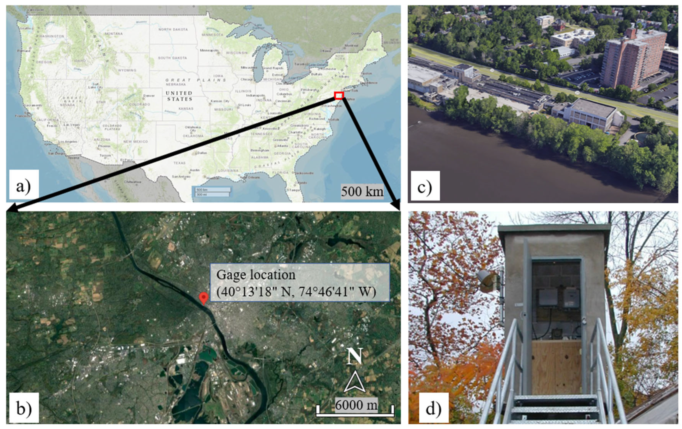
Figure 2.
Pipeline of the EDA and LSTM prediction tasks illustrates how the activities are linked from the data preprocessing steps to the model deployment stage. The steps are further categorized into their distinct group namely transformer, estimator, and evaluator.
Figure 2.
Pipeline of the EDA and LSTM prediction tasks illustrates how the activities are linked from the data preprocessing steps to the model deployment stage. The steps are further categorized into their distinct group namely transformer, estimator, and evaluator.
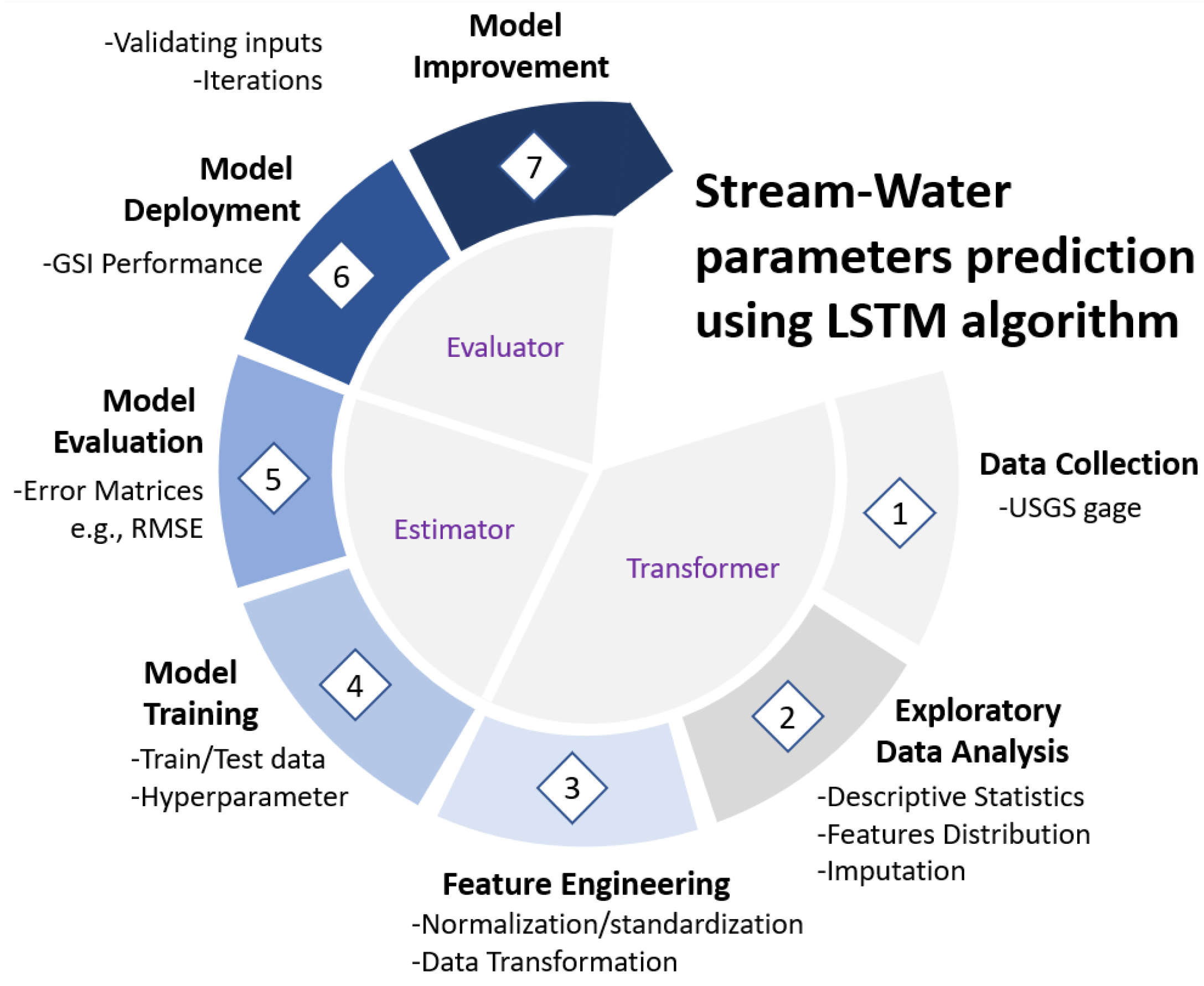
Figure 3.
Bivariate correlation coefficients among the SW variables represented by the correlation heatmap.
Figure 3.
Bivariate correlation coefficients among the SW variables represented by the correlation heatmap.
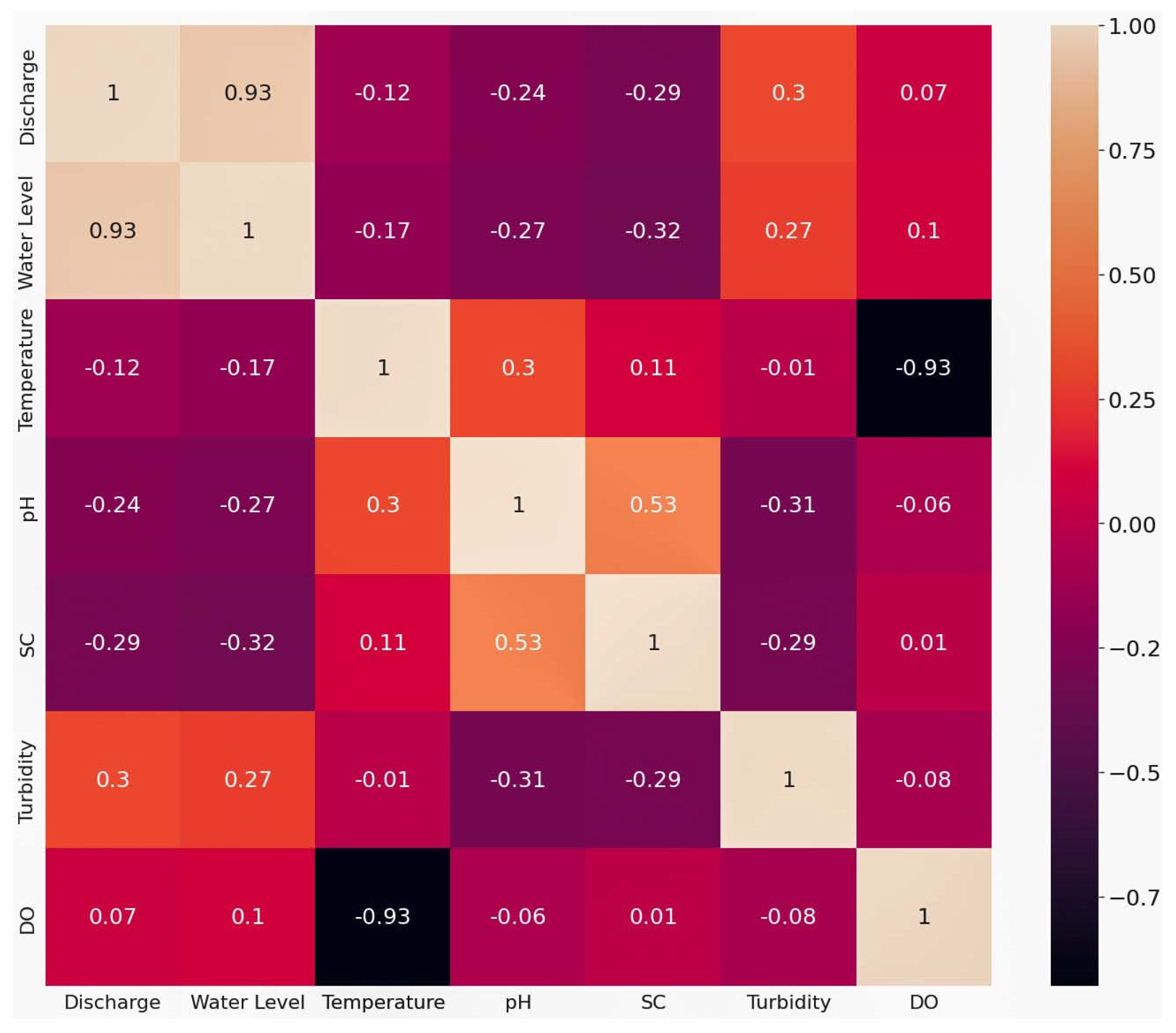
Figure 4.
Logarithmic transformation is applied to increase the normality of discharge and water level values.
Figure 4.
Logarithmic transformation is applied to increase the normality of discharge and water level values.
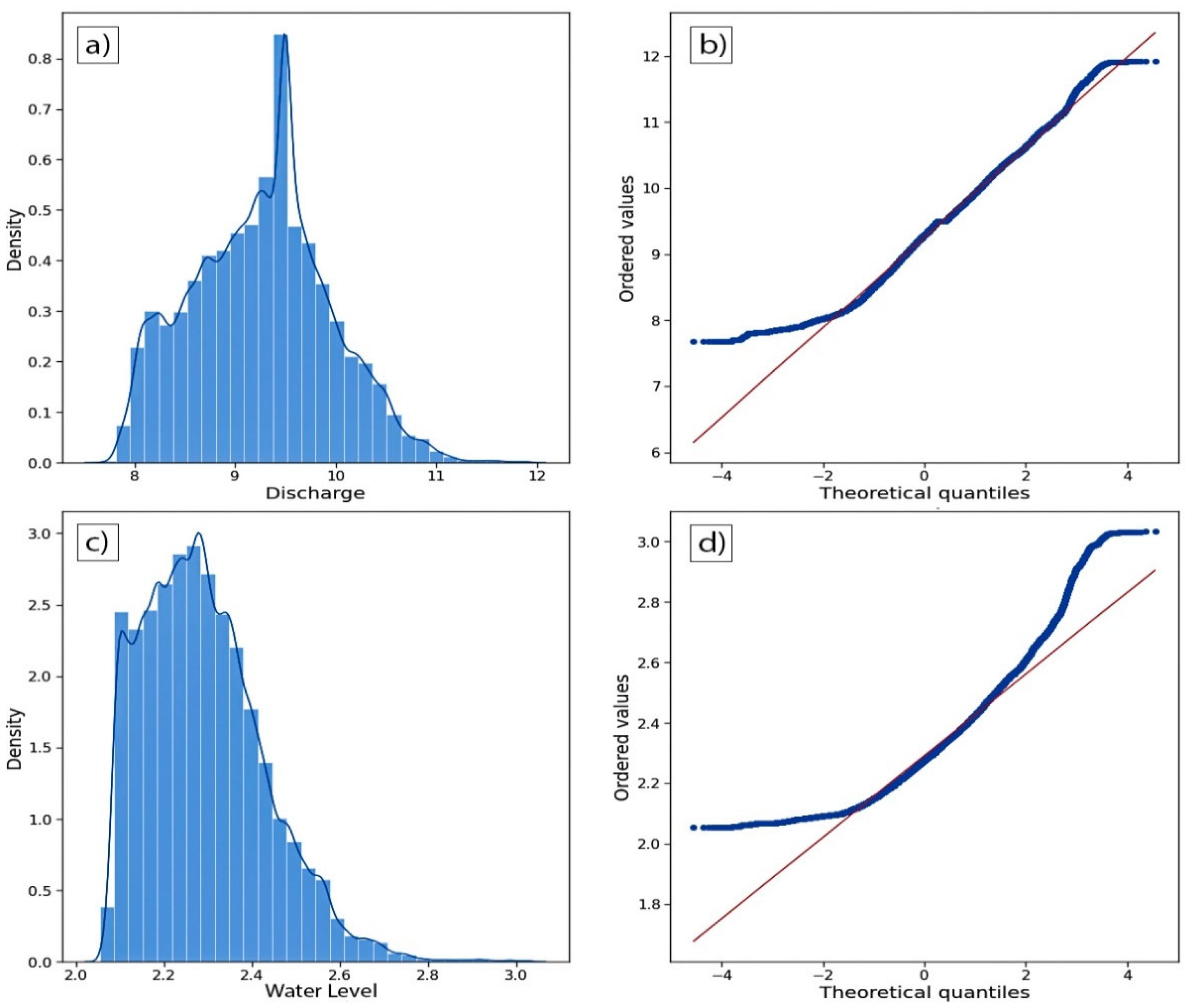
Figure 5.
Schematic representation of a LSTM architecture.
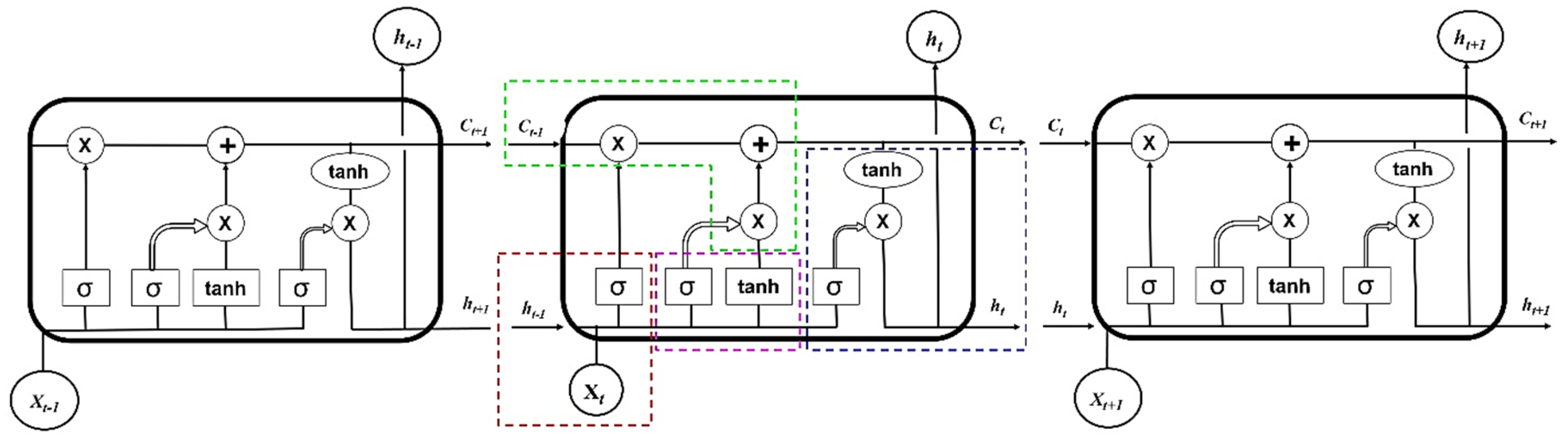
Figure 6.
Distribution of observed value from the gage records (dashed blue lines) and predicted values from LSTM model for the SW variables, discharge (a), water level (b), temperature (c), DO (d), pH (e), turbidity (f) and SC (g) with train/ test split (orange.
Figure 6.
Distribution of observed value from the gage records (dashed blue lines) and predicted values from LSTM model for the SW variables, discharge (a), water level (b), temperature (c), DO (d), pH (e), turbidity (f) and SC (g) with train/ test split (orange.
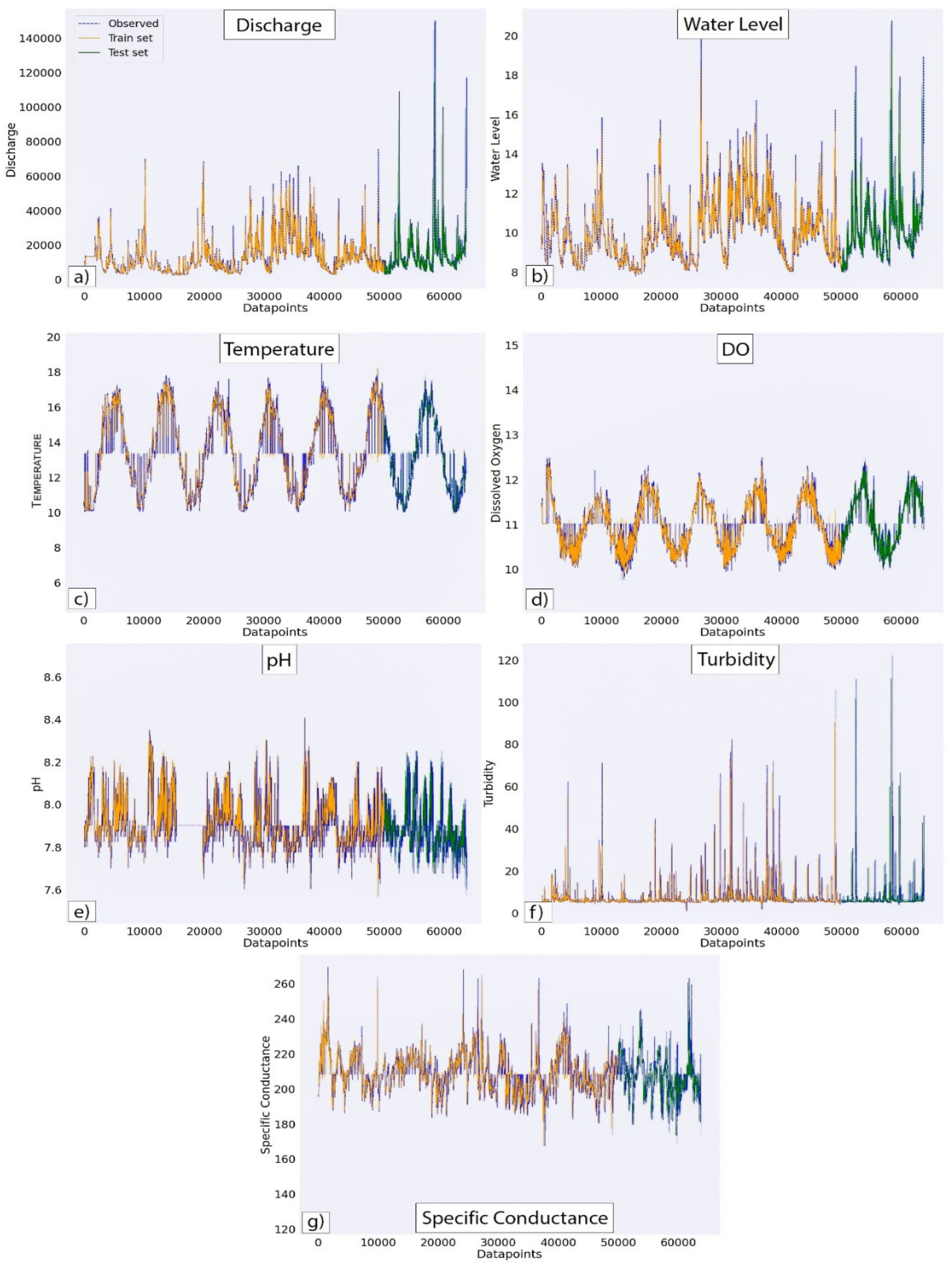
Figure 7.
Improvement of the model prediction capability with the increase in the number of epochs for the train and test set. RMSE value is the indicator of the model performance.
Figure 7.
Improvement of the model prediction capability with the increase in the number of epochs for the train and test set. RMSE value is the indicator of the model performance.
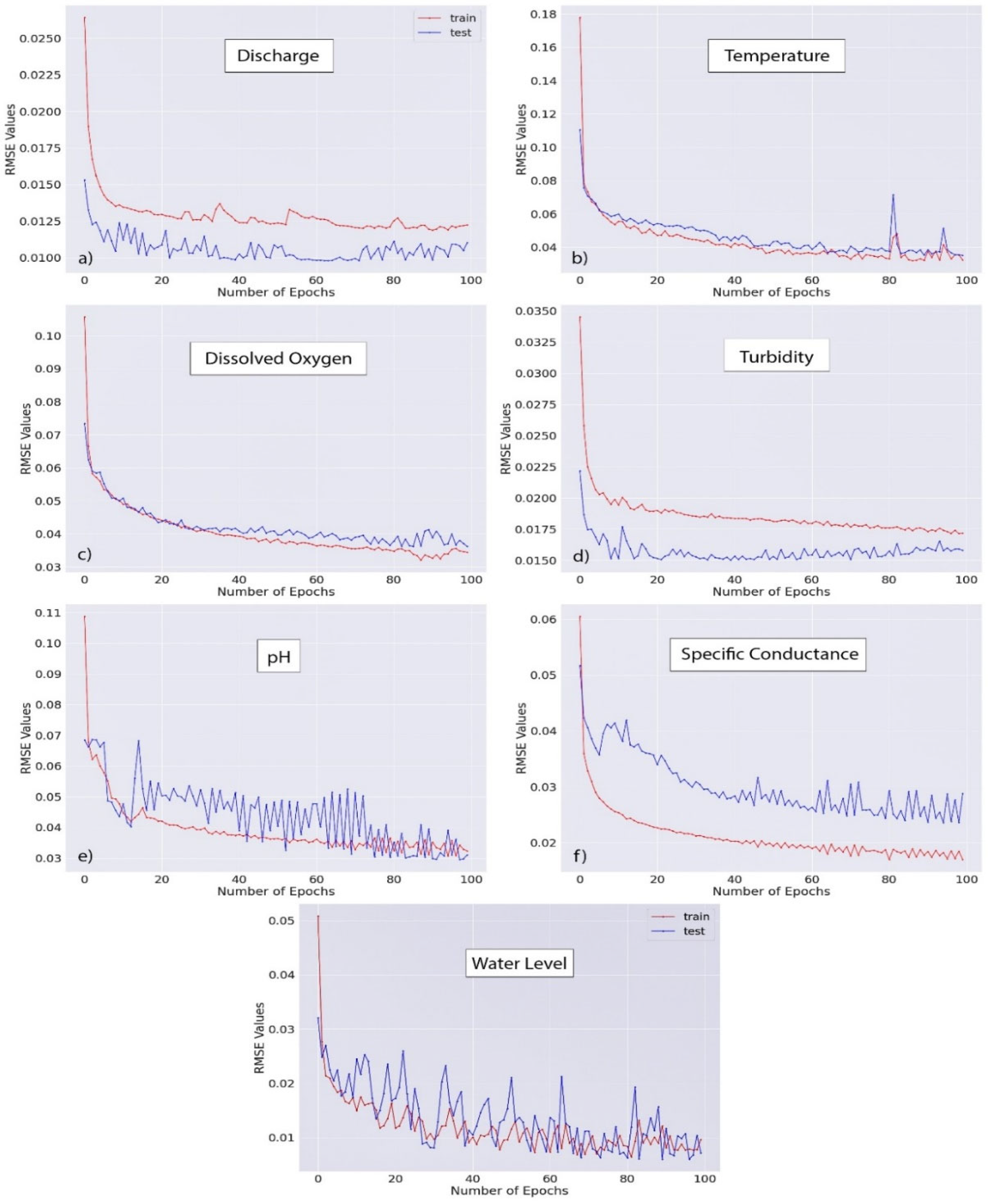
Figure 8.
Error matrices for various lead times for LSTM neural network model to predict discharge.
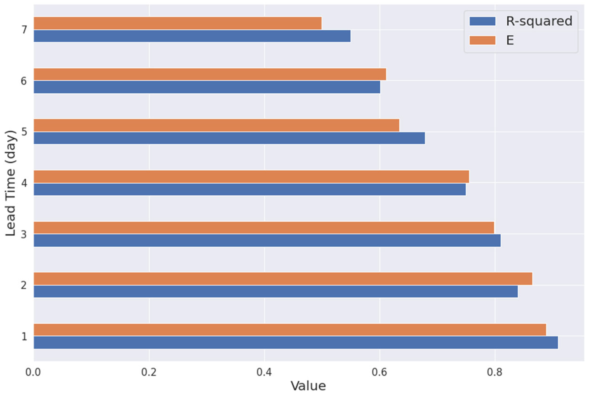
Figure 9.
Model performances are presented using the scatterplot of the standardized observed and predicted discharge values from LSTM model and the histogram of the distribution of the difference between the observed and predicted values of the SW parameters.
Figure 9.
Model performances are presented using the scatterplot of the standardized observed and predicted discharge values from LSTM model and the histogram of the distribution of the difference between the observed and predicted values of the SW parameters.
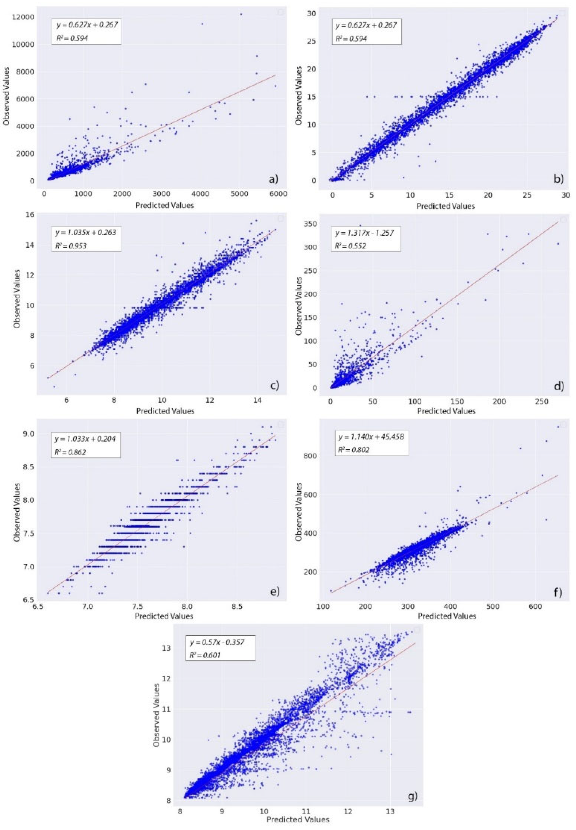
Figure 10.
Change in the error matrix, R^2values with the increase in the number of epochs batch, and neurons.
Figure 10.
Change in the error matrix, R^2values with the increase in the number of epochs batch, and neurons.
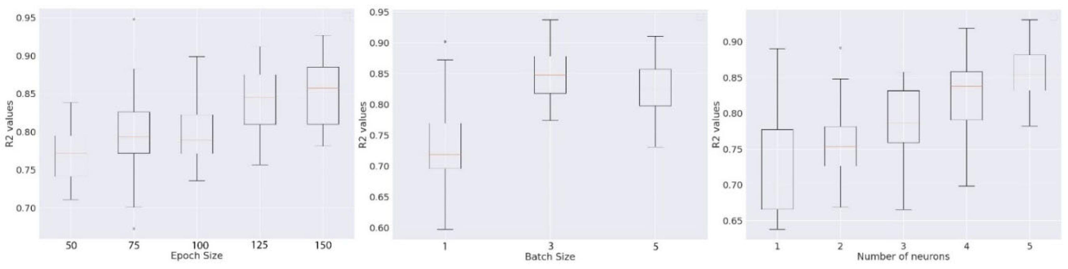

Table 1.
List of the SW variables used for EDA and predictive analysis with LSTM model.
| SW Parameters | Unit | Descriptions |
|---|---|---|
| Discharge | ft3/s | Quantity of stream flow |
| Water Level | ft | Stream water height/level at the gage location |
| Temperature | ℃ | Sensor-recorded temperature in ℃ at the gage |
| Dissolved Oxygen (DO) | mg/L | The amount oxygen dissolved in the SW. |
| Turbidity | FNU | Measure of turbidity in Formazin Nephelometric Unit (FNU) |
| pH | - | the acidity or alkalinity of a solution on a logarithmic scale |
| Specific Conductance (SC) | μS/cm | Measure of the collective concentration of dissolved ions in solution |
Table 2.
Descriptive Statistics of the SW variables.
| Count | Mean | Std | Min | 25% | 50% | 75% | Max | |
|---|---|---|---|---|---|---|---|---|
| Discharge (ft3/s) | 255066 | 13265.43 | 10657.91 | 2150 | 6240 | 10800 | 16100 | 150000 |
| Water Level (ft) | 255066 | 9.98 | 1.47 | 7.8 | 8.89 | 9.73 | 10.73 | 20.76 |
| Temperature (℃) | 255066 | 13.35 | 4.43 | 0 | 12.02 | 13.58 | 15.01 | 31.30 |
| pH | 255066 | 7.90 | 0.208 | 6.6 | 7.00 | 8.23 | 9.16 | 9.71 |
| SC (μS/cm) | 255066 | 208.19 | 22.23 | 49 | 201.11 | 208.64 | 221.09 | 453 |
| Turbidity (FNU) | 255066 | 6.44 | 6.54 | 0.2 | 5.61 | 6.44 | 7.29 | 469 |
| DO (mg/L) | 255066 | 11.02 | 1.11 | 6 | 11.02 | 11.07 | 12.67 | 16.90 |
Disclaimer/Publisher’s Note: The statements, opinions and data contained in all publications are solely those of the individual author(s) and contributor(s) and not of MDPI and/or the editor(s). MDPI and/or the editor(s) disclaim responsibility for any injury to people or property resulting from any ideas, methods, instructions or products referred to in the content. |
© 2023 by the authors. Licensee MDPI, Basel, Switzerland. This article is an open access article distributed under the terms and conditions of the Creative Commons Attribution (CC BY) license (http://creativecommons.org/licenses/by/4.0/).
Copyright: This open access article is published under a Creative Commons CC BY 4.0 license, which permit the free download, distribution, and reuse, provided that the author and preprint are cited in any reuse.


