1. Introduction
This study investigates the funding liquidity and the money market at the rate of interest and the evidence of India and the relationship between the Indian financial crisis. The financial system to produce the deposit reserve rate to manage the funding liquidity and the system to manage the discussing and the Indian financial system to produce the funding liquidity and the demand in the supply of Liquidity is proposed in this study. The Liquidity of money and the impact of the usual conception of the interpretation of the assuming and the distinction of the Liquidity and the factor to produce the market, which invested the contrast and therefore the stability of the money liquidity index calculation, were proposed.
The proposed idea helps make the effect of the Liquidity for the money shock evaluation. The policy and the Liquidity manage the further maintenance of the system to produce the attempt for the little management of the Liquidity and critical factor to producing the computer experiments, and the matching functions have been enabled. This can be exposed in the future proposed system to produce the evaluation of the system to produce the liquidity theory. This Liquidity handling and prediction theory manages the reserves of the money and the Liquidity of the policy balance sheet for both the adoption of the non-conventional factor for the efficiency and the effectiveness of the lower bound and the monetary of the issuance for the fiscal transfer. In this study, the minimum and maximum Liquidity boundaries manage the banks' cash exchange.
They are implementing this in the currently proposed system, employing banking and modern money, enabling liquidity with the financial factor. From the consideration, this study concentrated on identifying suitable liquidity risks related to the banking sector. Primarily relates to various liquidity crises and the appropriate measures of Liquidity, as well as the appropriate liquidity factors that influence financial performance. Here, the primary restriction is regarded to be Liquidity. Here, the financial performance services and their related state are calculated defectively using the liquidity ratios. This research employs the computation for consistency index approach to satisfy this performance service status forecast.
Regarding the price movement in the stock market, liquidity index-based prediction was combined. When the price fluctuates, trading and market transparency are impacted by Liquidity. The greedy technique for evaluating the factors most significantly impacted by the liquid index is used to regulate this trade and prevent market transparency of the liquidity index. Thus, this study elaborates on 25 fundamental financial elements contributing to the advanced greedy approach. Each Panther will have a definite liquidity crisis when coupled with the tractor. The minimum and maximum Degrees of matching are calculated whenever the liquidity crisis variables mix with the fundamental financial element. This computation establishes the precise, Plugin, subsume, and fail conditions that the various elements influenced the Liquidity. Finally, the analysis of the factors influencing Liquidity concerning the fundamental financial element and the liquidity issue is completed. Finally, the results were concluded with a successful reasonable outcome based on the Degree of matching and their effectiveness in locating liquidity elements. This study used a variety of financial criteria to identify the actual cause of Liquidity based on the Degree of matching results. This research article has the following contribution fulfilled by the proposed system of liquidity crisis determination. This research answers the following questions about good financial performance services. The research contribution is listed as follows
To discover appropriate liquidity risks concerns to a variety of financial criteria
To scale various Liquidity enhancing factors and analyze the implied dependencies among them
Create the procedural aspect of the proposed Liquidity management schema to find the Liquidity Ratios
Handle the various actual financial growth factors in the Liquidity management
To assess the liquidity risk while affecting the financial management crisis
The formation of the article is as below; Chapter 1 discussed the introduction of making an impact on common financial factors affecting liquidity ratio based on a greedy approach through price movement in the stock market. Chapter 2 discusses the literature review, which is relevant to Liquidity in the stock market. Chapter 3 discusses Proposed Liquidity crisis system model for fulfilling the impact on common financial factors affecting Liquidity. Finally, the conclusion references are mentioned at the end of the article
2. Literature Review
Degryse et al. (2016) propose the legal impact of Liquidity in a firm's stock. The process of managing the trading regulations and the implementation of market abuse directives on the Dutch stock market has been proposed [
1]. The symmetric legal trading for the impact of the permanent price has been increased. The price-sensitive information of the liquidity measure manages the European regulations. In addition, trading data has been proposed for Dutch companies. In addition, future trading-related factors that will happen in the stock liquidity can be proposed in the future research proposal; by implementing this in the currently proposed system, the regulation-based factor for the Liquidity has been maintained in the outside trading.
Yan et al. (2021) have proposed the fluctuation, the trend analysis, and the identification of the Liquidity in china and the stock market factor for the trend identification of the system. The process of cap stocks and the identification of the fluctuation and the facial market has been proposed using the trend entropy for the fractal market has been proposed to the china's trend markets [
2]. The identification of the stochastic rate and the trendy factor for the fluctuation and the fractal market has been proposed. The entropy dimension and identifying the trend to manage the lower factor for a tendency to reach the exponent has been evaluated. By implementing this in the currently proposed system, the efficiency of the facial entropy method has been evaluated.
Bencivenga et al. (1996) investigated the stock markets and their portfolios for liquidity for the size and the surrounding of the market in the market events [
3]. The process of managing the faster reversal and the idiosyncratic and the large stocks for analysing the market events for the significant market events. The process of managing the market-related events and forming the system to produce during the events is proposed. The investors and the implications, which enable the market during the idiosyncratic risk of the events, are done. The average movements of the system and the standard liquidity measures have been enabled and evaluated in this process. By implementing this in the currently proposed system, the portfolio for the investors and the Liquidity have been proposed.
Lu-Andrews et al. (2017) investigation of the secondary Liquidity market has been proposed in this manuscript [
4]. In addition, the long gestation of the investigations and the Liquidity of the system, which transmits the data for the absolute return and the equilibrium for the Liquidity in the market, has been proposed based on the improvements of the financial liquidity markets. The process of capital investments and the welfare of the high level of activity and the condition which enables the improvements of the financial markets have been proposed for the investments technologies of the system. The composition of the capital stock and the efficiency of the capital stocks has been proposed. The liquidity measures and the equilibrium saving can be improved by involving this in the currently proposed system.
Luo et al. (2021) have proposed the construction of an artificial stock market based on the multi-agent model. The behaviour of market volatility, Liquidity, and the efficiency of the strategy of the average price has been proposed [
5]. The market's longest liquidation and the system's volatility have been proposed. The efficiency of the most negligible impact and the absolute return for the analysis of the system has been enabled, for the extended memory factor for the absolute return has been proposed. The strategy of VWPA and the discovery of its efficiency and the volatile factor for the absolute returns have been proposed for the extended memory discovery has been proposed. By evolving this in the volatility of the most negligible impact of the absolute returns and the long memory of the market liquidity has been proposed.
González et al. (2011) discussed the liquidity introduction, which is based on the mean-variance and the selection of the portfolio, which belongs to the alternative risk of the Liquidity of the significance and the Liquidity of the low levels of the liquidity function, is proposed [
6]. The performance of estimating the mean-variance and the strong effects and the tangency of the Liquidity are proposed. Thus the choice and the effects of the Liquidity of the mean-variance have been proposed for the portfolio performance, and the preferences of the relatively of the system have been proposed. By implementing this in the currently proposed system, the portfolio and the sharp ratio factor for the risk levels can be proposed.
The value of the liquidity information and the marginal value of the Liquidity has been proposed by Kelly et al. (2007). the standard equilibrium solution for the distributors and the advantage of the reformulation analysis has been proposed for finding the liquidity information have been proposed [
7]. The price information n and the finding of the shadow price have been proposed for the marginal information, and the system's liquidity for the martingale factor has been proposed. By implementing this in the currently proposed system, the finding of the liquidity Doob factor for the information advantage can be proposed to interpret the marginal value.
The sale price and the selling price of the optimal and the selling price creditors, which elaborates the creditors of the former case and the high price of the price inflation and the failure of the default chain, have been enabled [
8]. The corporation management and the various adoption of Liquidity and liquidation are done. By involving this in the currently proposed system, the generalization of the higher price of equilibrium of buyers and the examination of the application and the interpreted factor has been proposed Degryse et al. (2016).
3. Proposed Liquidity Crisis System Model:
Xiang et al. (2011, August) take Liquidity Constraints to enhance the New Rural Old-Age Pension Program to improve Human Capital Investment. The liquidity theory was taken by Shen et al. (2005) to consume the Dispatch liquidity to handle the deregulated environment. The Liquidity is measured by Yang et al. (2006, June) against the Futures Market liquidity [
26]. This might be a chance to increase the excess Liquidity on the suggested choices of many users. Hence Xu et al. (2008, October) Suggested many Choices Eliminate Excess Liquidity. This analysis is done by Liu et al. (2009, September) Liquidity Analysis. This analysis is handled the Liquidity Risk against the Private Equity Fund Investment. the Fuzzy Evaluation Model is also used to Predicting Liquidity Ratio using Kong et al. (2020, December). This predicting liquidity ratio is eliminated in the mutual funds—ensemble learning the controls the boosting market liquidity. Cyclic trading is also elaborated by Eidenbenz et al. (2012, September) by peer-to-peer systems. This system impacted excess Liquidity, and this domestic food price inflation Analysis is also discussed by Yang et al. (2011, June). Xiao et al. (2011, November) inflation Analysis also affects the Exchange Rate, Excess Liquidity to Inflation, Foreign Reserve Growing, Liquidity Shock, and Stock Market Fluctuation. This statement of comprehensible work deals with Liquidity management using Liquidity Index [
12]. The Liquidity index was calculated based on the consistency index. The consistency index (C) impacts tick size reduction against the consistency index. The lower consistency index shows the international Liquidity, inflation and exchange rate, market liquidity, and efficiency. Wherever the stock index futures consume the lower consistency index, the default probabilities of stock futures index become lower [
35]. Perhaps the liquidity risk prediction and identification, liquidity creation, and resource fragility point out the liquidity risk because detecting the factor always influences market liquidity with the help of network-based computational techniques [
53]. To determine the consistency index of liquidity failures during a following systemic occasion [
27].
In terms of liquidity risk, the liquidity measurement is measured based on liquidity risk prediction and identification. Liquidity measurement helps reduce the liquidity risk against the existing liquidity index. Let us consider Consistency Index (C) from the Consistency Index (C) terminology. Whenever Consistency Index (C) becomes higher; the liquidity index should automatically become high. Hence, the market's capacity accommodates reasonably sizable market orders without materially affecting the security's price. This security's price accommodated the price fluctuations of a commodity between zero and one. The different futures contracts redeem the price fluctuations concerning the Total Turnover (TT). Before calculating the consistency index (C), the price fluctuations (pdf: Ѡ) must be calculated concerning the following equation 1 to 3
The consistency index (C) and price fluctuations (
) measures the following expressions to determine the number of shares traded during a particular time period,
Consistency Index (C) can be defined as follows
The following equation calculates the turnover defined by involuntary turnover (IVT) and voluntary turnover (VT). Hence the total turnover is.
When a process execution decides to quit reputation or retire from a live update, it is referred to as voluntary turnover. When a bank or government urges a process result to quit, it is called involuntary turnover [
61]. From this consideration,
Represents the price fluctuations concerning the 1 to n. Here n represents the time volatility consumption based on the market target. Hence, the total turnover result gives an appropriate Consistency Index (C) period. The Total Turnover (TT) should be calculated per equation (4).
Here the 'n' is the time based on the market target, T is time Volatility, t is the time taken for process execution market target,
is the marginal open interest.
The volume with respect to the time volatility. It varies from the t time taken for process execution market target and market target time [
54]. While considering the Future price (FP) on the consistency index (C) varies asymmetrically, the effects of positive and negative shocks will occur in the following consistency index calculation. Hence price fluctuations (
) is calculated busing
Hence the consistency index (C) will be calculated based on the market target, time and price volatility, voluntary turnover and involuntary turnover, and marginal open interest with respect to the time volatility of Liquidity is taken into consideration by the consistency index (C); the lower the consistency index (C) value Getting Liquidity back again the greater. Hence the equation () becomes,
To choose the correct price with respect to by the following terms and respective terms are used. For calculating the price volatility, this research uses three conditions for exploring the parameters such as time and price volatility
Condition1: positive time parameter and Null price parameter : NAGARCH
Condition2: Null negative time parameter and positive price parameter : COGARCH
Condition3: positive parameters time and price :
Firstly, this research build model of QGARCH, when the price volatility become noted with the various time and serious price parameter using the following equation,
QGARCH: The Quadratic GARCH (QGARCH) model typically reflects asymmetric impacts of positive and negative shocks [
13]. At the same time, this research uses the quadratic generalized autoregressive conditional heteroscedasticity on the serious price volatility at various time and null price parameters concerning the quadratic variation (vq).
Then, this research build model of COGARCH, when the price volatility become noted with the various time and Null price parameter using the following equation 7,
- b.
COGARCH:
COGARCH: The continuous-time GARCH (COGARCH) model typically reflects symmetric and asymmetric impacts of continuous-positive and continuous-negative shocks [
55]. At the same time, this research uses the continuous-time generalized autoregressive conditional heteroskedasticity on the serious price volatility constant time and price and time parameters treated like.
When the standard price volatility become noted with the various time and serious time parameter, uses the following equation,
- c.
NAGARCH:
Then, this research build model of NAGARCH while using the Nonlinear Asymmetric generalized autoregressive conditional heteroskedasticity on the serious price volatility constant time and price and time parameters treated like with the Asymmetric constrain [
17]. This might be stated that negative returns increase future volatility by a more significant amount than positive returns of the same price, which is reflected by the parameter often considered positive for stock returns.
Hence, the research chooses Condition1 to Condition3 when the consistency index (C) becomes more substantial in price volatility calculation [
47]. Each futures contract is determined based on the minimum and maximum delivery period that the commodity can end, which has a life of approximately less than one year. Because day trading is not based on long-term trends, there is a need to calculate the long-term trend of the overall market accurately so that the value of the market in day trading should be measured consistently and accurately with time trends [
22,
62]. The international futures values given are imprecise and require an empirical analysis of Liquidity. The chart for the long-term trend of the overall market in the daily trade this research mentioned illustrates this. Through this day trading, the continuous event forward distribution accurately follows the long-term trend of the overall market in the best possible way [
9,
14,
59]. So the futures market selects daily trading information of a series of contracts, including open price, close price, high price, low price, trading volume, and open interest, to describe the long-term price trend to analyse and minimize Liquidity in detail. How specific the adverse effects of the above three aspects are clearly explained below [
41,
45,
59].
3.1. Consistency Index Comparison
The capacity of a corporation to convert assets into cash or to get cash—through a loan or cash in the bank—to meet its short-term commitments or obligations is known as Liquidity. High Liquidity denotes a healthy, stable market where buyers and sellers may transact quickly, readily, and relatively [
9,
14,
19]. Given this, most development processes for cryptocurrency exchanges are concentrated on enhancing exchange platforms with tools that increase Liquidity. It is important to note that the Liquidity Index serves the same function as the Consistency Index. As the total of the consistency index and liquidity indexes will always equal one, they are connected to one another [
10].
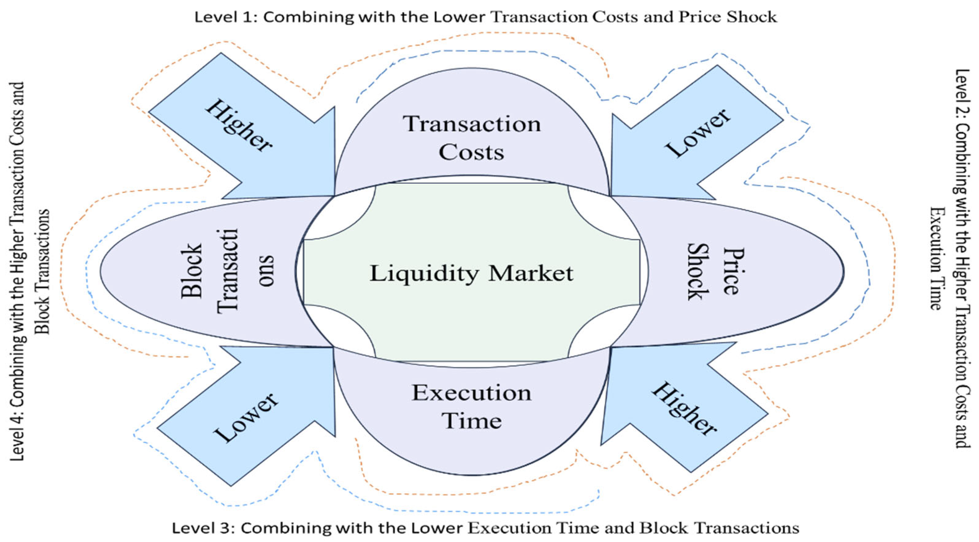
By combining the two, this research can see in
Figure 1. The ratio of a Consistency index to the difference between its liquidity limit and its Transaction Costs is known as the relative consistency or consistency index. The Consistency index determines the days needed to turn a company's trade receivables and inventory into Price Shock [
15,
19]. An organization's capacity to create the Block Transactions required to cover its present Execution Time is estimated using the Consistency index. The Consistency index should be treated as zero because it cannot have a negative value. The consistency ratio should be less than or equal to 0.1, and it is vital to evaluate conclusions if the consistency ratio is more than or equal to 0.1. The character will have a Consistency index of 1.0 if the minimum number of steps is the same as the observed number of steps [
18]. A character will have a Consistency index value of less than 1.0 if it is not entirely compatible with a Liquidity Market. The average Consistency index value across all characters is the Consistency index value of a Liquidity Market. Customers will always receive the same level of service from you, regardless of the person they talk with if you are consistent. Higher Consistency index ratios are often preferable to lower ones [
31]. A figure that is too high, however, can be problematic. When a corporation has a liquidity ratio of 1:1, the measured liquid assets cover all of its current obligations. Using a penetrometer is an easy way to assess the consistency of various goods. The measurement of grease penetration serves as a standard illustration of consistency determination [
36,
45].
This research calculates the complete process of the lower consistency index by the following five factors. Whenever this research calculates the consistency index, five factors consider for deciding consistent, in-depth events and their Liquidity [
25,
42,
48,
60]. Hence this research took 5 factors as (i). Tick size, (ii). Price movement restrictions, (iii). Trading restrictions, (iv). Allowable leverage, and (v). Market transparency. From these factors, this research decided the contribution regarding liquidity/ consistency index calculation. From this consideration, liquidity indexes are consistency indexes calculated based on the future price rate variation against Liquidity [
11,
16]. The following term helps manage the consistency index against Liquidity.
A futures contract is a cash-settled contract based on the Liquidity Index reference rate, which factors into the financial position. It acts as a one-day reference ratio of the cash valuation price of the Liquidity Index. Time Volatility combines the trading flow of primary market target and market target time exchanges during a one-hour calculation window [
21,
56]. Depth of Market (DOM) is a measure of supply and demand for liquid, tradable assets. It is based on the number of available buys and sells orders for a given asset, such as a stock or futures contract. The bigger the orders, the deeper or more liquid the market is considered to be.
3.2. Price Movement in Stock Market
The stock markets predict price movements by enabling future price prediction with the help of stock-based accurate future prices and time constrain [
20,
32]. This predicting method against the future price is described as per the description shown below
To concise the price movement in the stock market, this research maintains the following factors against the price movement. According to this formula, if this research can accurately predict a stock's future P/E and Earnings Per Share (EPS), this will concentrate the accurate future price with respect to the Historical Price, EPS Growth Rate Earnings Per Share and Predict Future Price [
46]. Hence, this research restricts the price movement to the following steps.
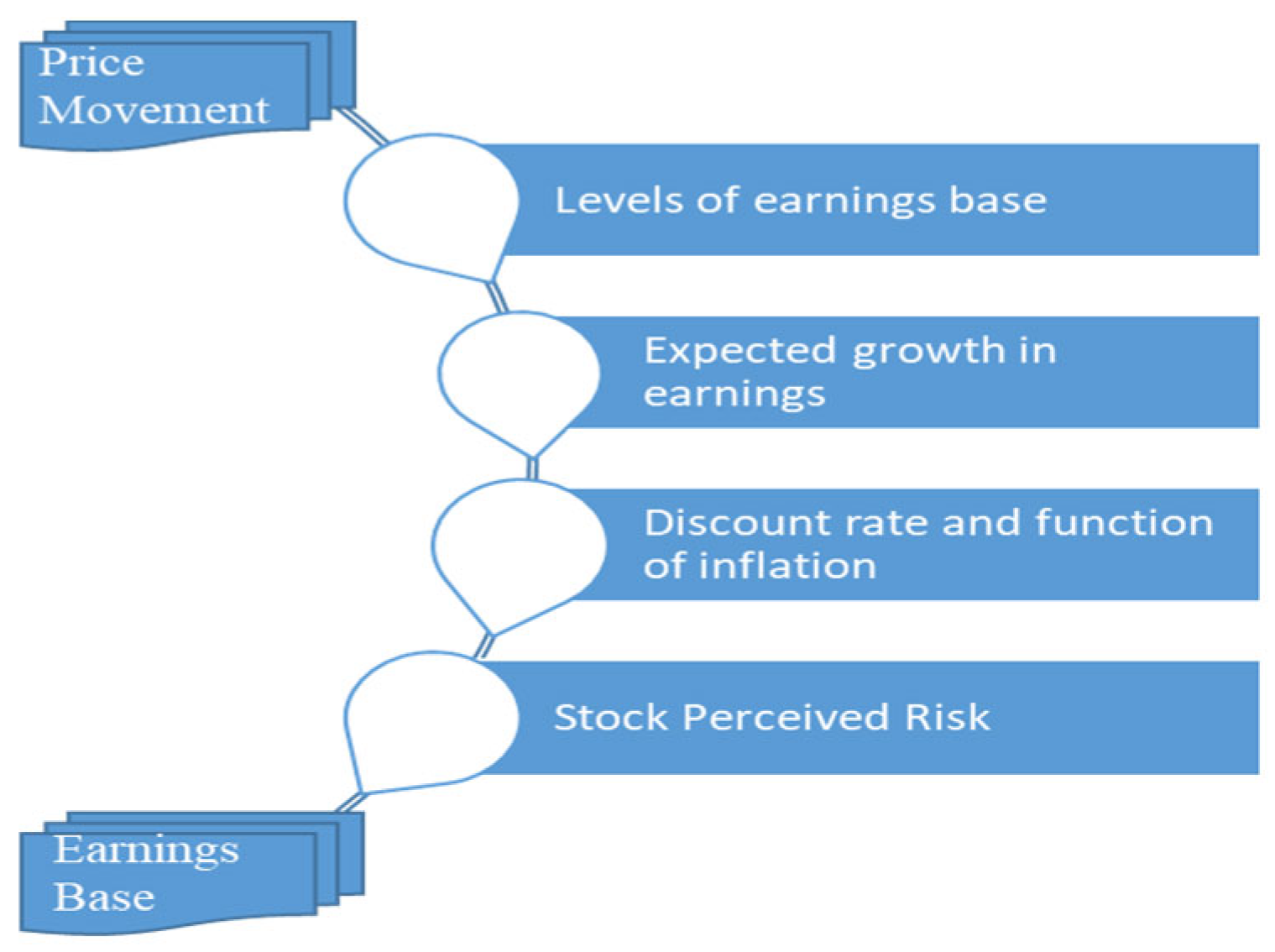
Figure 2 shows the first phase, which specifies the level of the earnings base and is represented by functions like growth rate, price, and time [
37,
49]. The earnings per share, excluding extraordinary items and discontinued operations, Liquidity per share, and dividends per share over the most recent countable price change in the stock market. The predicted increase in the earnings base is then adjusted in the following phase concerning the discount rate, which is a function of inflation. This inflation was determined based on how each participant felt about the stock's risk [
28].
Figure 1 shows the price movement in the stock market that declared concerning the price of women as well as earning place. Four levels of the process will be executed for calculating the price moment. Earning base took an expected growth input. When the input changes their growth, price mints are confined to two factors: discount rate and function inflation. The discount rate was manually modified concerning the liquidity rate. In addition, the function of inflation did not modify concerning Liquidity because Liquidity may change their serious time problem [
43,
56]. Hence, the function of inflation remains the same. However, when inflation reaches the stop perceived risk, the actual mean of perceived risk is calculated concerning their earning base. The following three processes are used to calculate the price movement limit after taking this into account [
33,
49].
In
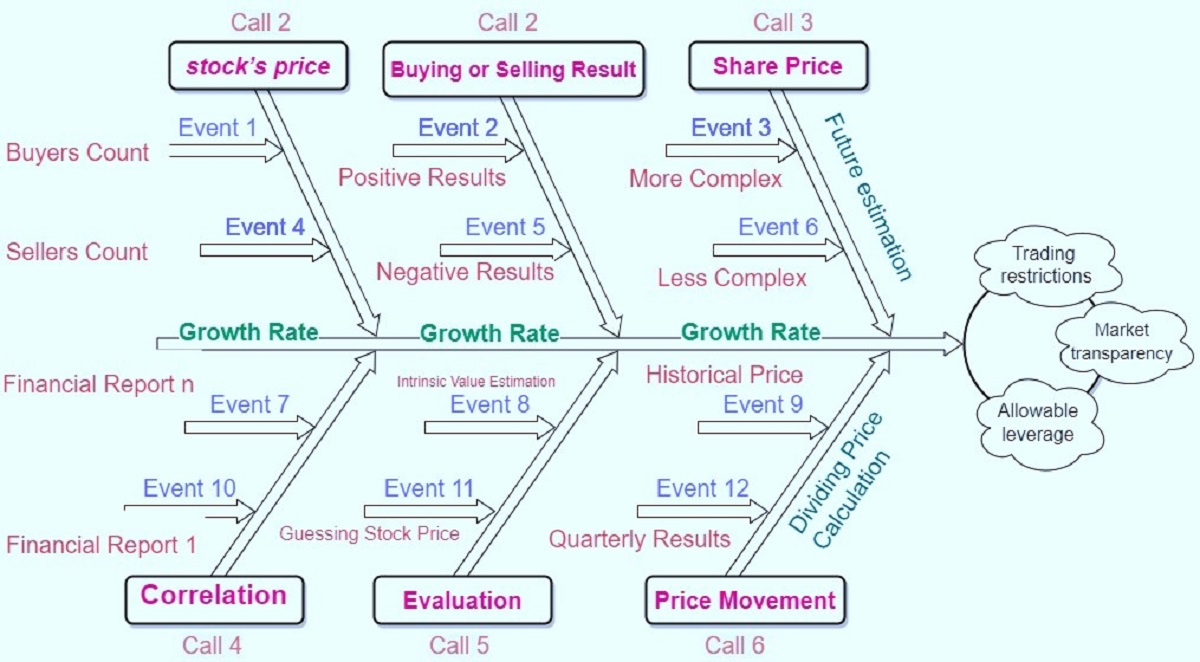
Figure 3, care is presented in the process of price moment estimation. Generally, this research calls for various aspects with their result against the growth rate and terms of Liquidity [
23,
44]. In such a case, call 1 and call 4 basically work based on correlation and stock price. Event 1, event 4, event 7, and event 10 determine actual stock price estimation concerning the correlation [
34]. These consolidated 4 events justify the actual growth rate concerning events. In call 1 whenever the bi account is fascinating, the stock price might be increased. Whenever the cell account is decreased, the stock price will decrease and change their respective stock price value [
57].
Is correlation will produce the highest growth rate in terms of financial reports. Similarly, when financial report 1 to financial report n is incremented for the correlation. Mean by at the 2nd, and 5th call were also applied to the actual price moment [
23,
58]. When the result changed from negative to positive, the buying or selling results were already examined for events five and 2. Hence, the buying and selling results affected or influenced their buying and selling results. In this case, the natural growth rate increased concerning the evaluation and buying and selling results [
39].
When this research considers the stock price concerning their intrinsic value estimation, a valuation report might be varied against the growth rate. Hence the process will consider the price moment and share price for incrementing the future estimation and dividing price calculation [
63]. Near the dividing price, a calculation concerning the price movement in terms of historical prices and quarterly results will be calculated. When the historical prices change automatically, the quarterly result will be e more impact against the dividing price calculation [
24,
45]. Moreover, event three and event six are estimated concerning the complex data when the complex more significant releases the events which will be executed automatically feature generation where is tea made the upcoming restriction [
29,
40,
50]. However, regarding more complex data handling on liquidity calculation, the growth rate gradually increases against future estimation until the process is applied to the next level of trading restrictions [
30].
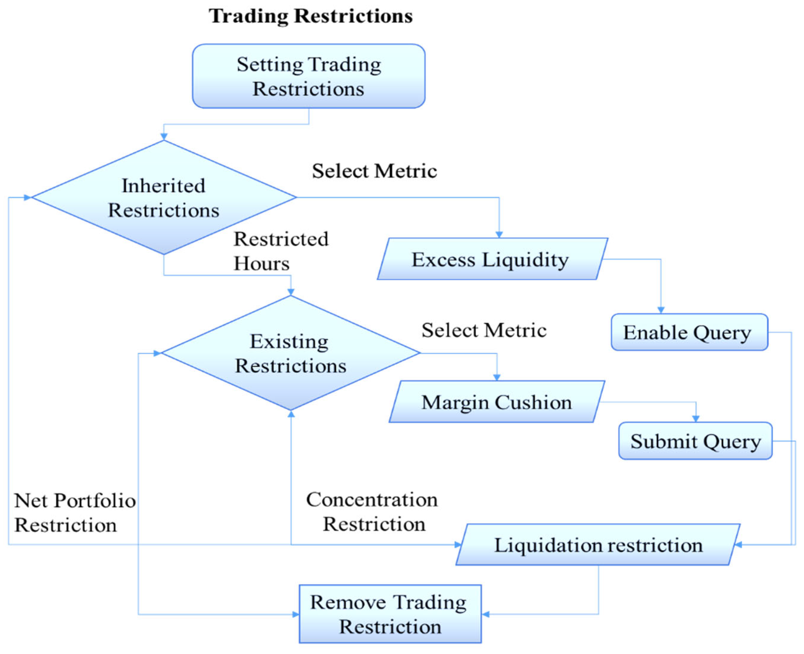
3.2.1. Trading Restrictions
A trade restriction is an artificial barrier to exchanging products and services between two or more nations (
Figure 4). It results from protectionism [
63].
3.2.2. Allowable Leverage
Based on a client's margin obligations with their broker, maximum leverage is the perfect position size allowed in a leveraged account. Under stock, investors are permitted to borrow up to 20% leverage, 30% leverage, 70% leverage, 75% leverage, 80% leverage, and 200% leverage of the value of a holding, although other brokerage companies may have stricter rules [
38].
20% leverage: If you trade two standard lots, this also means that the margin-based leverage is equal to the maximum real leverage a trader can use.
30% leverage: It is the process of 30:1 for trade among forex position change percentile with the maximum actual leverage trade.
70% leverage: A company's proper gearing level will depend on its industry and its corporate competitors' leverage level.
75% leverage: The loan amount and the property's current market value are compared using the Loan to Value (LTV) ratio, typically supported by an independent appraisal.
80% leverage: Purchasing a rental property illustrates financial leverage. Investors who put down less than 20% can borrow the remaining 80% of the purchase price from a lender.
200% leverage: It is the process of 200:1 for trade among forex position change percentile with the maximum actual leverage trade.
Maximum leverage is the most prominent position size permitted in a leveraged account based on a customer's margin requirements with their broker. Stock investors can borrow up to 50% of the value of a position under Reg T, but some brokerage firms may impose requirements that are more stringent.
Whenever a process is compared with its low latency or lower Consistency index where the Calculator concerning the allowable leverages, when the leverage value reaches the maximum 82%, will adopt all 200%, 80%, 75%, 70%, and 20% leverages. Once the leverage value gets 20% leverage, the consistency index will be low; otherwise, if the leverage value is 200%, this time also so, the consistency index will be low [
28,
51,
52]. Because that trade among the forest position change where remains same. The reason behind this constant value is that the consistency index must be varied concerning the price changes alone. But the price changes are not communicated or are irrelevant to the leverage value [
5]. The 20% leverage value and 200% leverage value give the same allowable leverage events and equality calculation for consistency index calculation. All other consistency leverage web calls are called maximum leverage [
45].
3.2.3. Market Transparency
The level of market transparency refers to how much information about market activities is made available to the public. The following are examples of essential data regarding a market routinely Published: Last-sale statistics. These reports include all trades' prices, quantities, and perhaps times as they happen [
34]. This research has to apply these five concepts to the proposed greedy approach. This greedy approach will give the exact point where the consistency index will be affected by the factor we take.
3.3. Multi Graph Possesses Greedy Approach
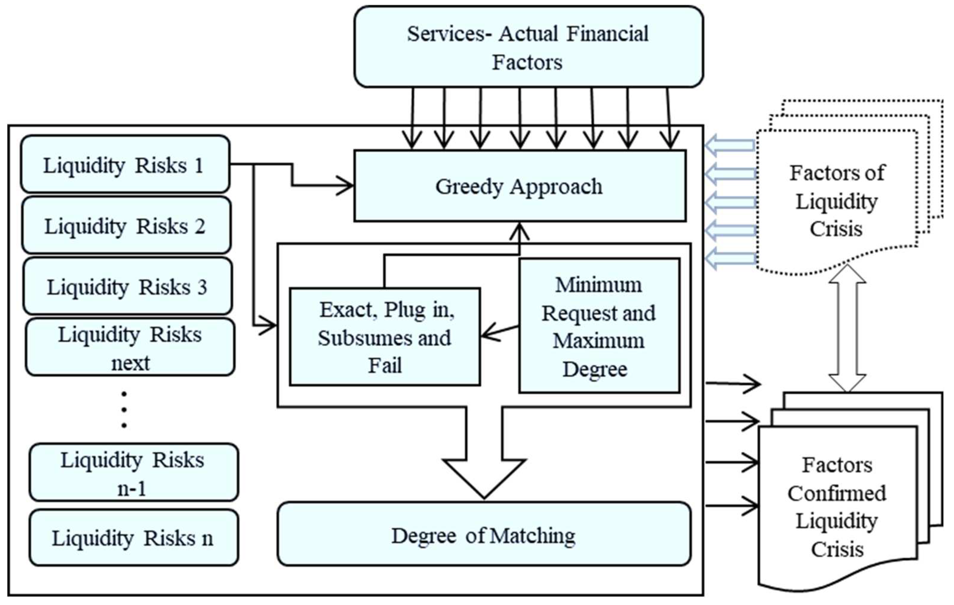
Paolucci's greedy approaches to the matchmaking process. The greedy approach is used to match the various factors of the consistency index for estimating the consistency index factor. The greedy approach consists of concept list matching whether the minimum request and maximum Degree of matching. Perhaps the minor Degree of matching is determined by how well the consistency index factor or output matches the input or output of the liquidity index factors. The mentioned method also examines all demands [
61]. The source algorithm for the matching process is the Paolucci algorithm that is currently in use. The Factors affecting (AF) the impact of liquidity crisis which is the Liquidity promoted by the consistency index factor, match Factors affecting (AF) the impact of liquidity crisis with the essential financial factors. Thus it can be assured that the matched financial factors entertained the requirements of the liquidity factors. The user liquidity facts are matched with the actual financial factors based on four Degrees of the match: exact, plugin, subsumes, and fail [
18].
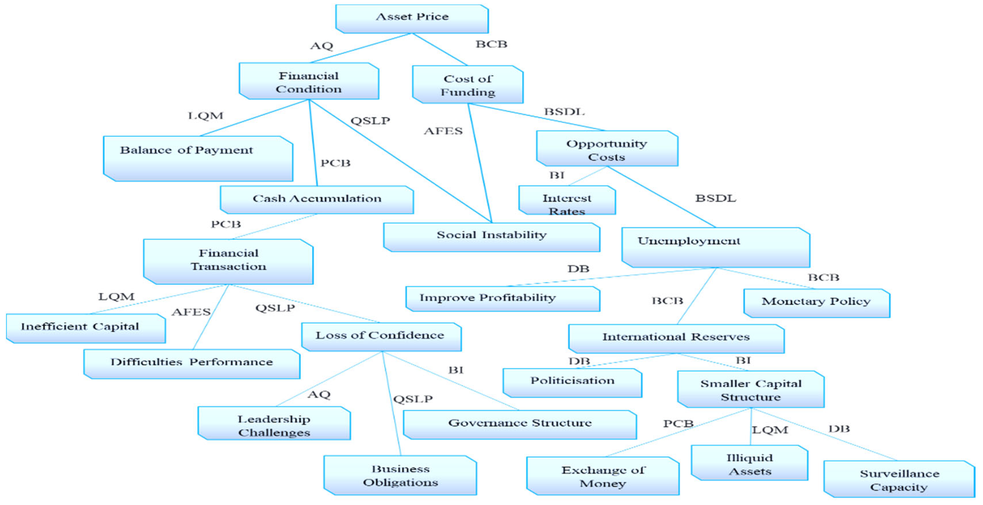
From
Figure 5, this proposed system greedy approach has 25 services available: likely Asset Price Bubbles and Unrealistic Valuations, and Balance of Payment Arising from the Fluctuations. In addition, Bank's Financial Condition, Centralise Cash Accumulation, and Dealing with Social Instability is also used. Moreover, the Except Unemployment and Cost of Funding, Financial Transaction or Commitment, Governance Structure, Improve Profitability, Inadequacy of International Reserves, and Increasing Level of Politicisation are processed Lack of Buyers Against the Inefficient Capital and Income. In addition to this, Leadership Challenges, Loss of Confidence In the Bank, Performance Evaluation Difficulties, Raises of Interest Rates, Reduce Debt against the Smaller Turn Capital Structure, Renders Expansionary Monetary Policy, Short-Term and Long-Term Business Obligations, Surveillance and Capacity-Building Activities, Transaction and Opportunity Costs, Transactions Involve an Exchange of Money, Transforming Illiquid Assets into Assets, Use The Ratio of Loans to Deposits and Widespread Defaults and Even Bankruptcies [
12,
43,
61] also available. These 25 essential financial factors are also called services behind the greedy approach. This approach is well compared with each factor that is a liquidity crisis. In this Era, the greedy approach got input from each service, and their services were compared with the factors of a liquidity crisis. Mainly the greedy approach is work based upon there are four results. Such as exact, plugin, subsumes, and fail. These four results are also called Degree of match results [
13]. These four factors comprise their minimum request and maximum Degree in terms of a liquidity crisis. When the medium that was and maximum Degree applied to the greedy approach, the services become exact, Plugin, subsumed, and failed. Finally, concerning the 'n' liquidity risk, the confirm factor is determined concerning the liquidity crisis. The following tips enhance how the process will execute and determine the actual reason behind the liquidity crisis. The following algorithm is used to propose a matching algorithm with the greedy approach. The proposed Matching Algorithm is shown in the below description [
38].
Matching Algorithm
Search (list of Liquidity Crises)
Result = Empty List
for each Actual Financial Factor in Liquidity Risks, 1 to n do
OutputMatch = match (Liquidity Crisis output, Actual Financial Factors output)
If (output Match = Fail) then
Skip Liquidity Crisis. Take the next Actual Financial Factor.
End if
Input Match = match (Liquidity Crisis input, Actual Financial Factors input)
if (inputMatch = Fail) then
Skip Liquidity Crisis. Take the next Actual Financial Factor.
end if
preconditionMatch=match(Actual Financial Factor precondition, Liquidity Crisis precondition)
if (preconditionMatch = Fail) then
Skip Liquidity Crisis. Take the next Actual Financial Factor.
end if
effectMatch=match(Liquidity Crisis effect, Actual Financial Factors effect)
if (effect match = Fail) then
Skip Liquidity Crisis. Take the next Actual Financial Factor.
end if
Result.Append(Liquidity Crisis, output Match, input match, preconditionMatch, effect match)
end for
return sort(Result)
end Search
3.3.1. Multi Graph Possesses Greedy Approach to Matchmaking
The proposed algorithm uses the input/output concepts for match-making. The Degree of match is explained as follows based on the Matching Algorithm (
Table 1):
From this
Table 1, the following results might be managing the stock exchange rate and actual finance factors with the liquidity factors.
Exact: If the concepts of the stock exchange rate and the actual finance factors are equivalent to the liquidity factors, then the Degree of the match is exact. Also, if the concepts of the stock exchange rate are the subclass of the stock exchange concepts, then the Degree of the match is exact.
Exact with PlugIn: If the concepts of the stock exchange rate and the actual finance factors are equivalent to the liquidity factors found for actual finance factors against precisely predicting actual finance factors, then the Degree of the match is exact. In addition, if the concepts of the stock exchange rate are the subclass of the concepts of the stock exchange, then the Degree of the match is Exact with PlugIn.
PlugIn: If the concept of the actual finance factors includes the concept of the stock exchange rate, then the Degree of the match is plug-in.
PlugIn with Subsume: If the concept of the actual finance factors includes the concept of the stock exchange rate with the Liquidity Factors Partially Found for Actual Finance Factors Predict Actual Finance Factors as PlugIn, then the Degree of the match is PlugIn with Subsume.
Subsume: If the concept of the stock exchange rate includes the concept of the actual finance factors, then the Degree of the match is subsuming.
Subsume with Fail: If the concept of the stock exchange rate includes the concept of the actual finance factors with the liquidity factors doubtfully found for actual finance factors predicts actual finance factors as Subsume, then the Degree of the match is Subsume with Fail.
Fail: If there is no match between the stock exchange rate and liquidity factors, the Degree of the match fails.
Fail with no Exact, no PlugIn, and no Subsume: If there is no match between the stock exchange rate and liquidity factors with the liquidity factors not possible to affect the actual finance factors, Predict Actual Finance Factors as becoming Fail then the Degree of the match fails.
This algorithm finds a high similarity between the stock exchange rate and the actual finance factor's liquidity factors in liquidity management [
14,
36]. This match-making algorithm helps in the dynamic liquidity management process of the stock exchange aspect of finance factors [
8]. The following
Table 2 describes the flexibility of maximum and minimum match-making
With minimum flexibility of match, the algorithm reduces false positives & increases false negatives, and with maximum flexibility, it increases false positives & reduces false negatives [
18]. The algorithm's result also depends approximately on the liquidity factors concepts.
Although Factors affecting (AF) the impact of the liquidity crisis are Asset Quality (AQ), Attraction of Funds from External Sources (AFES), Balance Sheet Demand and Liabilities (BSDL), Bank Image (BI), Bank's Capital Base (BCB), Deposit Base (DB), Level and Quality of Management (LQM), Peculiarities of the Customer Base (PCB), Quality of Securities and Loan Portfolio (QSLP). When liquidity factors are matched, the Paolucci algorithm does not clarify whether the liquidity factors are removed, thus leading to ambiguity and unreliable results [
12]. This limitation is explained through the following two scenarios. The Factors affecting (AF) the impact of liquidity crisis with Actual financial factors ontology is shown in
Figure 6.
-
A.
First Scenario
The concept from the advertisement is not removed from the candidate list after it has been matched (
Table 3 and
Table 4).
The Degree of matching is denoted as DOM, and the global Degree of the match is denoted as GDOM for Asset Price.
DOM (Financial Condition, Cost of Funding) = Exact
DOM (Cash Accumulation, Loss of Confidence) = Fail
DOM (Balance of Payment, Financial Transaction) = Exact
DOM (Politicisation, Capital Structure) = Fail
GDOM = exact
Financial condition, the Actual financial factor, is the subclass of the Asset Price. Therefore, the Degree of the match is Exact. Similarly, the balance of payment and financial Transaction is the subclass of price, and the Degree of the match is Exact. Since there is no relationship between Cash Accumulation, Loss of Confidence, and Politicisation, Capital Structure the Degree of match is Fail [
8,
19]. The Paolucci algorithm tries to find maximum similarity so the global Degree of match is Exact. The algorithm returns the Actual financial factor as the correct response to the Factors affecting (AF) the impact of the liquidity crisis. Two or more concepts from the financial factor match a single concept in Liquidity. The Liquidity represents a false positive value [
61].
-
B.
Second Scenario
The concept from the
financial factors is removed from the Actual financial factors list after it has been matched (
Table 5 and
Table 6).
DOM (Improve Profitability, International Reserves) = Exact
DOM (Monetary Policy, Interest Rates) = Exact
Profitability, Reserves, and Rates match Cost, and to reduce false positive values, Cost is removed from Actual financial factors concepts. Hence, the Degree of match is Fail. i.e., DOM (Inefficient Capital, Loss of Confidence) = fail
The algorithm returns that the Actual financial factor does not match the Liquidity factors. The Actual financial factor represents a false negative. The order of the Liquidity factors influences the matching process and changes the global Degree of the match with the result of Influenced Factors such as the Bank's Capital Base (BCB) and Balance Sheet Demand and Liabilities (BSDL). This research predicts the actual reason for improving Liquidity by improving the Cost of Funding and Opportunity Costs against the Factors affecting (AF) the impact of liquidity crisis limitations of the greedy approach [
17,
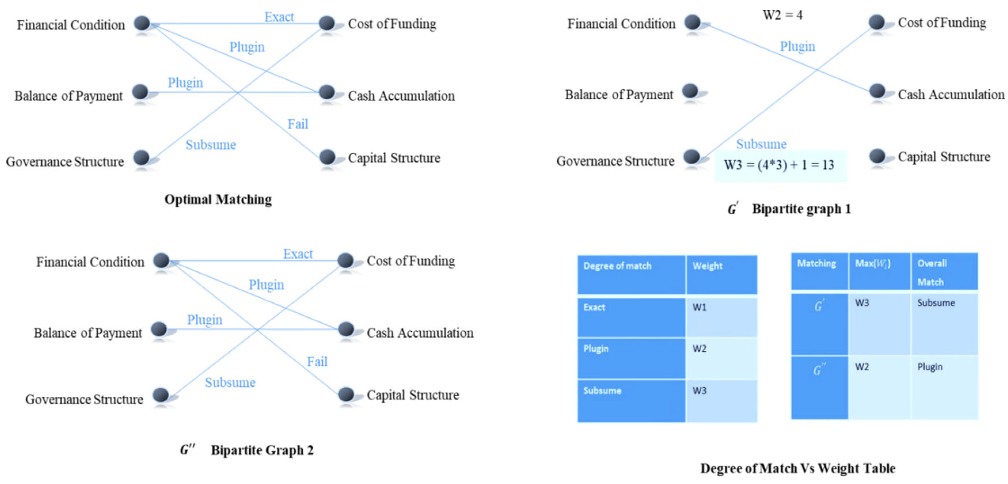
39]. The bipartite Graph-based match-making approach overcomes the excess proceeds. Based on the Factors affecting (AF) the impact of a liquidity crisis, the Actual financial factors are got the following DOM values [
18,
44]. That is indicated in
Table 7
3.3.2. Bipartite Graph-Based Approach
To overcome the problems of the greedy algorithm, match-making based on a bipartite Graph was proposed by Umesh Bellur et al . (2007) [
64]. This algorithm aims to achieve an optimal solution of concept matching. This algorithm uses a graph structure for match-making. A numerical weight (table) is assigned to the four degrees of the match. Thus to retrieve the Actual financial factors that match the Factors affecting (AF) the impact of the liquidity crisis Bipartite Graph is used. A bipartite Graph is a graph where the vertices set is partitioned into two sets. There exists an edge between vertices from one set to the other. No edge exists between two vertices of the same set. The user request is thus matched with the corresponding web services using a bipartite graph. Matching is done based on input and output factors.
Umesh Bellut et al. [
2] calculated the Degree of the match between the Actual financial factors and the Impact of Liquidity using the following algorithm. This approach is based on bipartite matching and Hungarian algorithm. The Hungarian algorithm finds the complete match. The optimal match is computed from the complete match by considering the minimum match.
The match-making process has two steps: constructing a bipartite Graph and optimal matching. The match-making process is explained through the following scenario. Let us consider the same Factors affecting (AF) the impact of liquidity crisis with Actual financial factors shown in
Figure 2. Actual financial factors are denoted as FF, and the Impact of Liquidity is denoted as IL(
Table 8 and
Table 9).
-
a.
Construction of Bipartite Graph
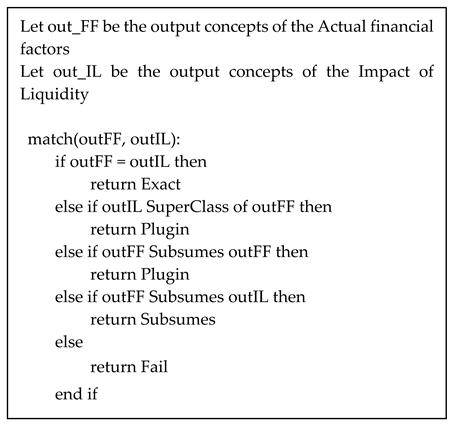
The Degree of the match is denoted as DOM. The Degree of matching between the output concepts is calculated using the algorithm shown in figure 3.
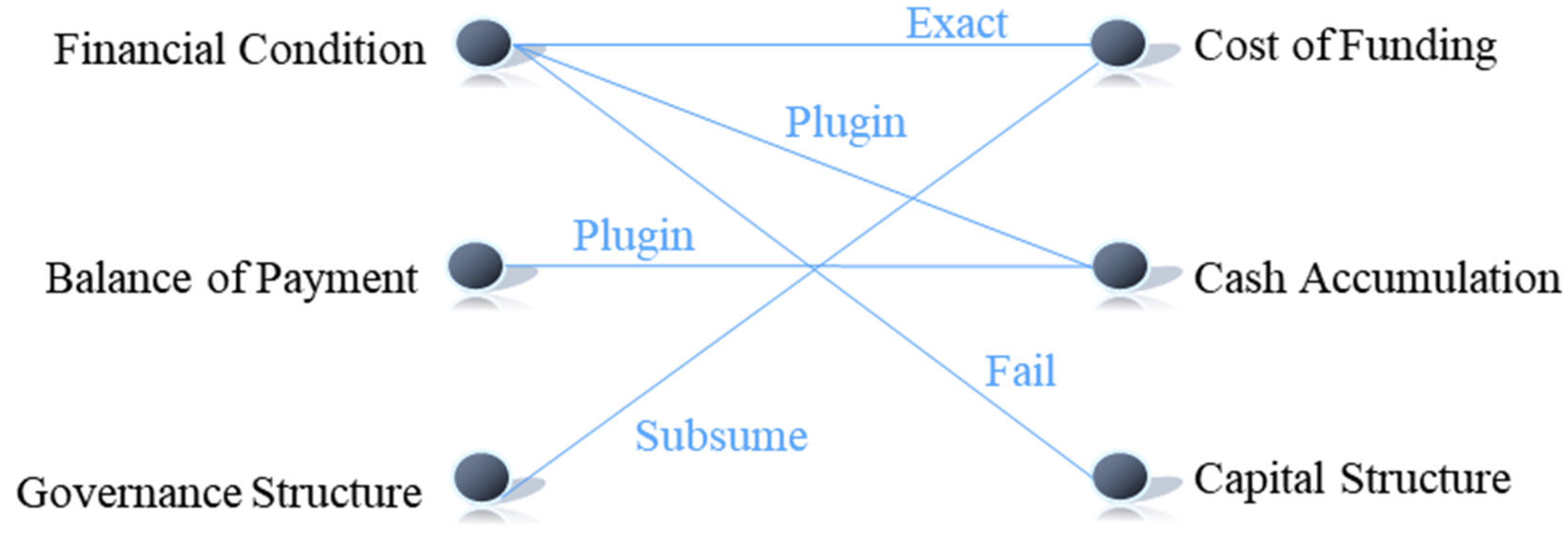
DOM (Balance of Payment, Financial Condition) = Exact
DOM (Balance of Payment, Cost of Funding) = Plugin
DOM (Balance of Payment, Governance Structure) = Fail
DOM (Cash Accumulation, Capital Structure) = Fail
DOM (Cash Accumulation, Financial Condition) = Plugin
DOM (Cash Accumulation, Governance Structure) = Fail
DOM (Financial Transaction, Financial Condition) = Subsume
DOM (Financial Transaction, Capital Structure) = Fail
DOM (Financial Transaction, Governance Structure) = Fail
The output concepts, out_FF = Balance of Payment and out_IM = Financial Condition, are equivalent, and their Degree of the match is Exact [
38]. Cost of Funding is the subclass of Balance of Payment, so their Degree of match is PlugIn. There is no match between Balance of Payment and Governance Structure, so their Degree of match is fail. Financial Transaction is a Financial Condition, so their Degree of match is Subsume. Similarly, the Degree of match is found for other output concepts. The Bipartite Graph is shown in
Figure 7. Let the output query concepts be
and output advertisement concepts be
-
b.
Enhanced Optimal matching
The following numerical weights are assigned for each Degree of the match. Each edge is now labeled with the corresponding numerical weights.
The above
Figure 8,
(Plugin) is chosen as the optimal match because of W2 < W3. The Degree of match plugin is returned. Thus match-making using bipartite Graph works. The performance of this algorithm is better than the greedy approach [
51]. This type of bipartite Graph-based algorithm regulates false positives and false negatives. The accuracy, plug-in, sub, and failure levels of the fundamental elements that impacted the liquidity consistency index were identified using this computation. To successfully and reasonably identify the liquidity variables, the search ultimately identifies the fundamental financial component and the factor impacting the Liquidity concerning the liquidity crisis. It also considers their efficacy and significance in doing so [
52]. This research discovered a trustworthy source of Liquidity with the aid of numerous financial aspects based on the most recent matching findings, which is highly fertile ground for future study.
