
Submitted:
03 January 2023
Posted:
06 January 2023
You are already at the latest version
Abstract
Downward short-wave (SW) solar radiation is the only essential energy source powering the atmospheric dynamics, ocean dynamics, biochemical processes, etc. on our planet. Clouds are the main factor limiting the SW flux over the land and the Ocean. For the accurate meteorological measurements of the SW flux one needs expensive equipment - pyranometers. For some cases where one does not need golden-standard quality of measurements, we propose estimating incoming SW radiation flux using all-sky optical RGB imagery which is assumed to incapsulate the whole information about the SW flux. We used DASIO all-sky imagery dataset with corresponding SW downward radiation flux measurements registered by an accurate pyranometer. The dataset has been collected in various regions of the World Ocean during several marine campaigns from 2014 to 2022, and it will be updated. We demonstrate the capabilities of several machine learning models in this problem, which are multilinear regression, Random Forests, Gradient Boosting and convolutional neural networks (CNN). We also applied the inverse target frequency (ITF) re-weighting of the training subset and the approach of pre-classification in order to raise the SW flux approximation quality. We found that the CNN is capable of approximating downward SW solar radiation with higher accuracy compared to existing empiric parameterizations. We also found that the ITF reweighting of the training subset increases the approximation quality substantially. The estimates of the SW radiation flux using all-sky imagery may be of particular use in case of the need for the fast radiative budgets assessment of a site.
Keywords:
downward solar radiation
; clouds
; machine learning
; deep learning
; convolutional neural networks
; ResNet
; all-sky imagery
; Random Forests
; Gradient Boosting
1. Introduction
Solar radiation is the main source of energy on Earth [1]. It is also of great significance for biogeochemical, physical, ecological, and hydrological processes [2,3]. Cloud cover, in turn, is the main physical factor limiting the downward solar radiation flux [4,5,6]. Cloud cover during the day reduces the influx of solar radiation to the Earth’s surface, and significantly weakens its outgoing longwave radiation at night due to backscattering [7]. This entails corresponding changes in other meteorological quantities. The functioning of agriculture, transport, aviation, resorts, alternative energy enterprises and other sectors of the economy, in one way or another, depends on the amount and shape of clouds.
There are two options for flux estimation in modern models of climate and weather forecasts. First is a physics-based modeling of radiation transfer through two-phase medium (clouds) which includes modeling of multi-scattering taking into account the microphysics of cloud water drops [8] and aerosols. This option is computationally extremely expensive. Alternatively, one may use parameterizations which are simplified schemes for approximating environmental variables using only routinely observed cloud properties, such as Total Cloud Cover (TCC), cloud types and cloud cover per height layer. The existing parametrizations are empirical and were proposed years and decades ago based on observations and expert-based assumptions [9,10]. As a result, they may not take into account the entire variety of cloud situations occurring in nature, which may lead to a reduced quality of approximation of downward SW solar radiation flux.
Our goals are to get computationally cheaper estimations of downward solar radiation flux and to study flux dependence on structural characteristics of clouds. The aim of this study is to improve the accuracy of existing parameterizations of downward SW radiation flux. In this study, we assess the capability of machine learning models in the scenario of statistical approximation of radiation flux from all-sky optical imagery. We solve the problem using various machine learning (ML) models within the assumption that an all-sky photo contains complete information about the downward SW radiation.
There are a number of studies on the forecasting of downward SW radiation using advanced statistical models namely Machine Learning models [3,10,11]. Most of them deal with the time series of SW radiation flux measured directly by an instrument (radiometer), thus, in case of the need for a low-cost assessment package, one cannot apply this approach. There are also a number of ML methods published for estimating other useful properties of the clouds, e.g., total cloud cover [12,13] or cloud types [14,15,16]. To our best knowledge, there is only one study demonstrating the capabilities of statistical modeling in the problem of the estimation of downward SW radiation flux [17]. In this study, though, the statistical relation is demostrated between the semantically rich meteorological features (solar zenith angle, surface albedo, hemispherical effective cloud fraction, ground altitude and atmospheric visibility) and the SW radiation flux. In contrast with this study, we model the statistical relations between the raw all-sky imagery and the SW radiation flux. We do not propose to infer any of semantically significant features of the all-sky visual scene. The only semantically meaningful feature we propose to use is the sun altitude which we compute using the position, date and time of observations.
The rest of the paper is organized as follows: in Section 2, we describe the dataset that we use in our study; in Section 3, we introduce the methods we exploit in our study for approximating the SW downward radiation flux; in Section 4, we present and discuss the results of our study. In Section 5, we summarize the paper and present the outlook for further study.
2. Data
In this section, we present source data for our study. The problem we tackle is to map all-sky imagery to SW radiation flux using state of the art statistical models (a.k.a. machine learning models). We use a high-resolution fish-eye cloud-camera «SAIL cloud v.2» [13] to collect all-sky images, and the radiometer Kipp&Zonen CNR-1 to measure SW flux. In Figure 1, we present the equipment used to collect the data.
The source data we use in our study is the Dataset of All-sky Imagery over the Ocean (DASIO) [12] which we collect in marine expeditions starting from 2014. The regions covered in these missions include Indian and Atlantic oceans, Mediterranean sea and Arctic ocean. In this dataset, the exhaustive set of cloud types is present. DASIO contains over 1 500 000 images of skydome over the ocean accompanied with downward SW radiation flux measurements. SW solar flux is averaged in 10-second intervals, and the all-sky images are registered every 20 seconds. The viewing angle of the Kipp&Zonen CNR-1 sensors is 180° in both vertical planes. The viewing angle of the cloud-camera is similar. Photos taken from the fisheye cloud-camera have high enough resolution to resolve fine clouds structural details (1920*1920 px). White balance and brightness of photos are adjusted automatically for the most comfortable visual experience.
In our study, we employed a subset of DASIO. The size of the training subset was more than 1 000 000, and the size of the test subset was more than 350 000 images (see Table 1). In other words, the ratio of the volumes of test and training subsets is 1:3. A particular sampling strategy was involved when we split the dataset into training and testing subsets. Since the period of images acquisition is 20 seconds, the visual scene of the skydome did not change substantially between subsequent images. Thus, they are strongly correlated. In this case, subsequent images may be considered one with small perturbations, thus, they should not be massively distributed across training and testing subsets. This isuue may arise in case of random per-image sampling. In order to avoid this issue, we applied temporal block-folded sampling. To be precise, we applied random sampling using hours of observations instead of objects (images) themselves.
Figure 1c also demonstrates a mask we applied to each photo, which filters our visual objects that are not related to the subject of our study. In addition, to train the models, we used only data obtained during daylight hours, when the Sun altitude exceeded 5 °, and the radiation flux exceeded 5 .
We state the problem as follows: for each observation of the whole sky registered in an all-sky image, one needs to approximate the value of the short-wave radiation flux, which is supervised in the form of CNR-1 measurements. In terms of Machine Learning (ML) approach, it is a regression task with the scalar target value. We used mean squared error as a loss function for the ML models exploited in this study. We also charaterize the quality of the solutions using mean absolute error (MAE) measure.
2.1. Inverse target-frequency (ITF) re-weighting of training subset
In target value distribution (see Figure 2), one may notice a strong predominance of data points with low SW flux. Thus, the dataset is strongly imbalanced w.r.t. target value. This kind of issue may cause reduced approximation quality [18,19]. In our study, we chose to exploit the approach of weighting the data space (following the terminology of [19]). In order to improve the approximation skills of our models, we balance the train dataset using inverse-frequency re-weighting. We name it inverse target frequency (ITF) re-weighting. To be precise, we made the weights of individual examples of train dataset to be inversely proportional to the frequency of target values:
where i enumerates inter-percentile intervals from 0-th to 99-th; are the inter-percentile intervals of empiric target value distribution, and is a number of inter-percentile intervals. Here, the less target frequency, the more inter-percentile interval , thus, the more are the weights of the examples. In order to illustrate the approach we propose, we present percentile-wise vertical lines in Figure 2, so one may notice uneven inter-percentile distances in the cumulative distribution function figure.
In addition to the ITF re-weighting, we also propose the scheme for controlling the re-weighting strength using coefficient:
Here, one may notice, that the closer to 1, the stronger re-weighting is applied. In case of , there is no re-weighting, meaning . Given the form of the weights and , one may notice that their expected value is exactly . Coefficient is a hyperparameter of our re-weighting scheme which is optimized during hyperparameters optimization stage.
3. Methods
In our study, we used two approaches: the classic approach and the so-called end-to-end approach with convolutional neural network employed.
Within the classic approach, we examined the following ML models: multilinear regression and non-parametric ensemble models Random Forests (RF) [20] and Gradient Boosting (GB) [21,22,23]. Within this approach, we built a real-valued feature space of images consisting of 163 features. In particular, the following statistics were calculated for each color channel (Red, Green, Blue, Hue, Saturation and Brightness) of an image: maximum and minimum values; mean and variance; skewness, kurtosis and percentile set from 5 to 95 with increment of 5, as well as 1 and 99 percentiles. We also used the feature of sun altitude calculated using geographic position and UTC time of images. Training and inference of the "classical" ML models of our study was performed using scikit-learn [24] implementations of these models.
Within the end-to-end approach, we did not computed any of expert-designed features. In contrast, we applied Convolutional Neural Network (CNN) [25] directly to the images. We also applied heavy images augmentation meaning strong alterations of average brightness. We also added spatially correlated gaussian noise. We applied these color-wise augmentations in order to increase the generalization ability of the CNN, and also in order to train the network to infer a flux link to the spatial structure of cloudiness instead of average brightness fo an image. Within this end-to-end neural networks-based approach, we also used the feature of sun altitude. The structure of the CNN exploited in our study is shown in Figure 3. As one may see in this figure, input data are the all-sky RGB imagery resized to the resolution of 512x512 px. In order to speed up the learning process and to improve the quality of the approximation, we employed Transfer learning approach [26]: a pre-trained version of the ResNet50 [27] network is used, which was pre-trained on the ImageNet [28] dataset. The output of the ResNet50 convolutional sub-network is a 2048-dimensional vector. We concatenate sun altitude to this vector, thus the resulting vector is 2049-dimensional. We then apply a fully-connected sub-network to it. The structure of this sub-network is presented in Figure 3. The output of this subnet is real scalar value approximating the flux. We used Adam algorithm [29] for optimizing our CNN. Training and inference of the CNN we presented was implemented with Python programming language [30] using Pytorch [31], OpenCV [32] for Python and other high-level computational libraries for Python.
In both the ensemble models (RF and GB), we exploited in our study, there are hyperparameters besides the re-weighting coefficient we presented above. Among them are the number of ensemble members in RF and GB; the maximum depth of the trees of the ensemble, etc. The CNN is also characterized by a number of hyperparameters: its depth, the width of fully-connected layers in fully-connected subnet, the hyperparameters of Adam optimization procedure, and also the magnitude of data augmentation transformations. We employed Optuna framework [33] for hyperparameters optimization (HPO). During the HPO stage, the quality of each model initialized with a sampled hyperparameters set is assessed within K-fold cross-validation (CV) approach with . Due to strongly correlated examples (all-sky images) that are close in temporal domain, we ensured the independence of train and validation CV-subsets using Group K-fold cross-validation approach where groups are hourly subsets of all-sky images. In case of RF and GB models, we assess the mean RMSE measure as well as its uncertainty within the Group K-fold CV approach.
4. Results and discussion
In this section, we present the results of our study. To assess the quality of our models, we used root mean square error (RMSE) measure. In order to estimate the uncertainty of the quality measures, we trained and evaluated each model several times (typically, 5-7) and estimated the confidence interval of 95% significance level, assuming the RMSE being normally distributed random variable. Also, the visual representation of the results is given in the form of value mapping diagrams (Figure 4), where the correspondence between approximated and measured flux values is presented in a form of points density. In Figure 5, we present the errors histograms for the models involved in our study.
In Figure 4, one may see that the models generally underestimate high fluxes and overestimate low fluxes. It is also clear that multilinear model approximates the flux worse than other models, which is supported by the RMSE measures in Table 2. The results of CNN are the best among others in terms of formal RMSE measure as well as approximated-to-measured values mapping diagram.
In our study, we built and trained four ML models to approximate the downward shortwave radiation flux. We found, that the quality of the CNN, which was built within the end-to-end approach, is the best compared to other models and also to existing SW radiation parameterizations known from the literature [9,34]. In Table 2, we present the quality of our models assessed after the hyperparameters optimization. We also provide RMSE estimates of the parametrizations as a reference. One may also observe that parameterizations error strongly depends on the amount of cloudiness: the higher Total Cloud Cover (TCC) the higher a parameterization error. We provide the errors range in brackets for parameterizations known from the literature.
In Figure 5, we also demonstrate error distributions for each ML models of our study. In the CNN error distribution (Figure 5d), one may see that the neural network is prone to underestimate the SW flux slightly. Also, it is clear that erors distribution tails are pretty heavy for both RF and GB models, and are light for CNN. These features of errors distribution for our models are also in agreement with the variance of errors that are presented in Figure Table 2 in a form of RMSE (taking into account that the errors are zero-centered, thus RMSE is the square root of variance in this case.)
One may also observe that the ITF re-weighting did not make any difference in terms of RMSE quality measure. Neither Random Forests, nor Gradient Boosting for Regression models did not demonstrated any performance improvement due to ITF re-weighting.
One may also note, that the models we present demonstrate some issues. Multilinear regression is a fast model, however, it has the worst quality. RF and GBR demonstrate comparable quality and are relatively fast at inference time. At the same time, one may note non-smooth errors distribution in diagrams in Figure 4(b-e). We suppose that the regular drops of points density may be explained by decision-tree-based nature of these two ensemble models. One may also notice the outliers in these diagrams that may be of interest in forthcoming study. In this study, we did not filter the outliers comprehansively, thus there may be irrelevant imagery in the dataset that represent photographs of birds, glass dome cleaning operator, etc.
5. Conclusions and outlook
In this study, we presented the approach for the approximation of short-wave solar radiation flux over the Ocean from all-sky optical imagery using state of the art machine learning algorithms including multilinear regression, Random Forests, Gradient Boosting and convolutional neural networks. We trained our models using the data of DASIO dataset [12]. The quality of our models was assessed in terms of RMSE, approximated-vs.-measured flux diagrams and errors histograms. The results allow us to conclude that one may estimate downward SW radiation fluxes directly from all-sky imagery taking some well-known uncertainty into account. We also demonstrate that our CNN trained with strong data augmentations is capable of estimating downward SW radiation flux based on clouds’ visible structure mostly. At the same time, the CNN is shown to be superior in terms of flux RMSE compared to other ML models in our study.
Our method of flux estimation may be especially useful in the tasks of low-cost monitoring of downward fluxes of shortwave solar radiation, as well as in exploratory studies of territories for their placement. The solution of the presented problem makes it possible to obtain estimates of the downward SW solar flux based on model atmospheric data containing clouds characteristics, which may reduce the computational load of the radiation subroutine.
Our results suggest that there are outliers in DASIO dataset that may be filtered in forthcoming studies. The results also suggest that hyperparameters optimization of our CNN and ensemble models may help discovering better configurations including proper dataset re-weighting as well as more suitable CNN architecture.
In further studies, we plan to improve the approach of resampling and re-weighting. We also plan to approximate downward longwave solar radiation flux using the approach similar to the one presented in this paper. Also, modern statistical models of Machine Learning class provide opportunity for short-term forecasting of fluxes which may be useful in forecasting the generation of solar power plants.
Author Contributions
Conceptualization, Mikhail Krinitskiy and Sergey Gulev; Data curation, Vasilisa Koshkina, Nikita Anikin and Sergey Gulev; Funding acquisition, Sergey Gulev; Methodology, Mikhail Krinitskiy; Project administration, Maria Artemeva; Software, Mikhail Krinitskiy, Vasilisa Koshkina, Mikhail Borisov and Nikita Anikin; Supervision, Sergey Gulev; Validation, Vasilisa Koshkina, Mikhail Borisov and Nikita Anikin; Writing – original draft, Mikhail Krinitskiy and Vasilisa Koshkina; Writing – review & editing, Mikhail Krinitskiy and Maria Artemeva. All authors have read and agreed to the published version of the manuscript.
Funding
The research is funded by RFBR grant 20-05-00244 (development of ML and CNN algorithms) and by RSF grant 23-47-00030 (analysis of SW downward radiation fluxes). Optimization of hyperparameters of classical ML models was undertaken with the financial support of the Ministry of Education and Science of the Russian Federation as part of the program of the Moscow Center for Fundamental and Applied Mathematics under the agreement 075-15-2022-284.
Conflicts of Interest
“The authors declare no conflict of interest.“
Abbreviations
The following abbreviations are used in this manuscript:
| CNN | Convolutional neural network |
| DL | Deep learning |
| ML | Machine learning |
| SW | short wave |
| LW | long wave |
| DASIO | Dataset of All-Sky Imagery over the Ocean |
| RF | Random Forests |
| LR | Linear regression |
| MLR | Multilinear regression |
| GBR | Gradient Boosting for Regression |
References
- Trenberth, K.E.; Fasullo, J.T.; Kiehl, J. Earth’s Global Energy Budget. Bulletin of the American Meteorological Society 2009, 90, 311–324. [Google Scholar] [CrossRef]
- Stephens, G.L.; Li, J.; Wild, M.; Clayson, C.A.; Loeb, N.; Kato, S.; L’Ecuyer, T.; Stackhouse, P.W.; Lebsock, M.; Andrews, T. An update on Earth’s energy balance in light of the latest global observations. Nature Geoscience 2012, 5, 691–696. [Google Scholar] [CrossRef]
- Wu, H.; Ying, W. Benchmarking Machine Learning Algorithms for Instantaneous Net Surface Shortwave Radiation Retrieval Using Remote Sensing Data. Remote Sensing 2019, 11, 2520. [Google Scholar] [CrossRef]
- Cess, R.D.; Nemesure, S.; Dutton, E.G.; Deluisi, J.J.; Potter, G.L.; Morcrette, J.J. The Impact of Clouds on the Shortwave Radiation Budget of the Surface-Atmosphere System: Interfacing Measurements and Models. Journal of Climate 1993, 6, 308–316. [Google Scholar] [CrossRef]
- McFarlane, S.A.; Mather, J.H.; Ackerman, T.P.; Liu, Z. Effect of clouds on the calculated vertical distribution of shortwave absorption in the tropics. Journal of Geophysical Research: Atmospheres 2008, 113. [Google Scholar] [CrossRef]
- Lubin, D.; Vogelmann, A.M. The influence of mixed-phase clouds on surface shortwave irradiance during the Arctic spring. Journal of Geophysical Research: Atmospheres 2011, 116. [Google Scholar] [CrossRef]
- Chou, M.D.; Lee, K.T.; Tsay, S.C.; Fu, Q. Parameterization for Cloud Longwave Scattering for Use in Atmospheric Models. Journal of Climate 1999, 12, 159–169. [Google Scholar] [CrossRef]
- Stephens, G.L. Radiation Profiles in Extended Water Clouds. I: Theory. Journal of the Atmospheric Sciences 1978, 35, 2111–2122. [Google Scholar] [CrossRef]
- Aleksandrova, M.; Gulev, S.; Sinitsyn, A. An improvement of parametrization of short-wave radiation at the sea surface on the basis of direct measurements in the Atlantic. Russian Meteorology and Hydrology 2007, 32, 245–251. [Google Scholar] [CrossRef]
- Ebtehaj, I.; Soltani, K.; Amiri, A.; Faramarzi, M.; Madramootoo, C.A.; Bonakdari, H. Prognostication of Shortwave Radiation Using an Improved No-Tuned Fast Machine Learning. Sustainability 2021, 13, 8009. [Google Scholar] [CrossRef]
- Voyant, C.; Notton, G.; Kalogirou, S.; Nivet, M.L.; Paoli, C.; Motte, F.; Fouilloy, A. Machine learning methods for solar radiation forecasting: A review. Renewable Energy 2017, 105, 569–582. [Google Scholar] [CrossRef]
- Krinitskiy, M.; Aleksandrova, M.; Verezemskaya, P.; Gulev, S.; Sinitsyn, A.; Kovaleva, N.; Gavrikov, A. On the generalization ability of data-driven models in the problem of total cloud cover retrieval. Remote Sensing 2021, 13, 326. [Google Scholar] [CrossRef]
- Krinitskiy, M.A.; Sinitsyn, A.V. Adaptive algorithm for cloud cover estimation from all-sky images over the sea. Oceanology 2016, 56, 315–319. [Google Scholar] [CrossRef]
- Liu, S.; Duan, L.; Zhang, Z.; Cao, X.; Durrani, T.S. Multimodal Ground-Based Remote Sensing Cloud Classification via Learning Heterogeneous Deep Features. IEEE Transactions on Geoscience and Remote Sensing, I: 1–11. Conference Name. [CrossRef]
- Liu, S.; Li, M.; Zhang, Z.; Xiao, B.; Cao, X. Multimodal Ground-Based Cloud Classification Using Joint Fusion Convolutional Neural Network. Remote Sensing 2018, 10, 822. [Google Scholar] [CrossRef]
- Taravat, A.; Frate, F.D.; Cornaro, C.; Vergari, S. Neural Networks and Support Vector Machine Algorithms for Automatic Cloud Classification of Whole-Sky Ground-Based Images. IEEE Geoscience and Remote Sensing Letters 2015, 12, 666–670. [Google Scholar] [CrossRef]
- Chen, L.; Yan, G.; Wang, T.; Ren, H.; Calbó, J.; Zhao, J.; McKenzie, R. Estimation of surface shortwave radiation components under all sky conditions: Modeling and sensitivity analysis. Remote Sensing of Environment 2012, 123, 457–469. [Google Scholar] [CrossRef]
- He, H.; Garcia, E.A. Learning from Imbalanced Data. IEEE Transactions on Knowledge and Data Engineering 2009, 21, 1263–1284. [Google Scholar] [CrossRef]
- Branco, P.; Torgo, L.; Ribeiro, R. A Survey of Predictive Modelling under Imbalanced Distributions, 2015. arXiv:1505. 0165. [Google Scholar] [CrossRef]
- Breiman, L. Random forests. Machine learning 2001, 45, 5–32. [Google Scholar] [CrossRef]
- Prokhorenkova, L.; Gusev, G.; Vorobev, A.; Dorogush, A.V.; Gulin, A. CatBoost: unbiased boosting with categorical features. Advances in neural information processing systems 2018, 31. [Google Scholar]
- Ke, G.; Meng, Q.; Finley, T.; Wang, T.; Chen, W.; Ma, W.; Ye, Q.; Liu, T.Y. Lightgbm: A highly efficient gradient boosting decision tree. Advances in neural information processing systems 2017, 30. [Google Scholar]
- Chen, T.; Guestrin, C. Xgboost: A scalable tree boosting system. Proceedings of the 22nd acm sigkdd international conference on knowledge discovery and data mining, 2016, pp. 785–794.
- Pedregosa, F.; Varoquaux, G.; Gramfort, A.; Michel, V.; Thirion, B.; Grisel, O.; Blondel, M.; Prettenhofer, P.; Weiss, R.; Dubourg, V.; Vanderplas, J.; Passos, A.; Cournapeau, D.; Brucher, M.; Perrot, M.; Duchesnay, E. Scikit-learn: Machine Learning in Python. Journal of Machine Learning Research 2011, 12, 2825–2830. [Google Scholar]
- O’Shea, K.; Nash, R. An introduction to convolutional neural networks. arXiv preprint arXiv:1511.08458, arXiv:1511.08458 2015.
- Tan, C.; Sun, F.; Kong, T.; Zhang, W.; Yang, C.; Liu, C. A survey on deep transfer learning. International conference on artificial neural networks. Springer, 2018, pp. 270–279.
- He, K.; Zhang, X.; Ren, S.; Sun, J. Deep Residual Learning for Image Recognition. 2016, pp. 770–778.
- Deng, J.; Dong, W.; Socher, R.; Li, L.J.; Li, K.; Fei-Fei, L. Imagenet: A large-scale hierarchical image database. Computer Vision and Pattern Recognition, 2009. CVPR 2009. IEEE Conference on. Ieee, 2009, pp. 248–255.
- Kingma, D.P.; Ba, J. Adam: A Method for Stochastic Optimization. arXiv:1412.6980 [cs], arXiv:1412.6980 [cs] 2017. arXiv: 1412.6980.
- Van Rossum, G.; Drake, F.L. Python 3 Reference Manual; CreateSpace: Scotts Valley, CA, 2009. [Google Scholar]
- Paszke, A.; Gross, S.; Massa, F.; Lerer, A.; Bradbury, J.; Chanan, G.; Killeen, T.; Lin, Z.; Gimelshein, N.; Antiga, L.; Desmaison, A.; Kopf, A.; Yang, E.; DeVito, Z.; Raison, M.; Tejani, A.; Chilamkurthy, S.; Steiner, B.; Fang, L.; Bai, J.; Chintala, S. PyTorch: An Imperative Style, High-Performance Deep Learning Library. In Advances in Neural Information Processing Systems 32; Wallach, H.; Larochelle, H.; Beygelzimer, A.; Alché-Buc, F.d.; Fox, E.; Garnett, R., Eds.; Curran Associates, Inc., 2019; pp. 8026–8037.
- Bradski, G. The OpenCV Library. Dr. Dobb’s Journal of Software Tools.
- Akiba, T.; Sano, S.; Yanase, T.; Ohta, T.; Koyama, M. Optuna: A Next-generation Hyperparameter Optimization Framework, 2019. arXiv:1907. 1090. [Google Scholar] [CrossRef]
- Dobson, F.W.; Smith, S.D. Bulk models of solar radiation at sea. Quarterly Journal of the Royal Meteorological Society 1988, 114, 165–182. [Google Scholar] [CrossRef]
Figure 1.
Equipment we use to collect the data, and an example of all-sky optical imagery over the ocean: a) radiometer Kipp&Zonen CNR-1; b) cloud-camera «SAIL cloud v.2»; c) all-sky photo with mask.
Figure 1.
Equipment we use to collect the data, and an example of all-sky optical imagery over the ocean: a) radiometer Kipp&Zonen CNR-1; b) cloud-camera «SAIL cloud v.2»; c) all-sky photo with mask.
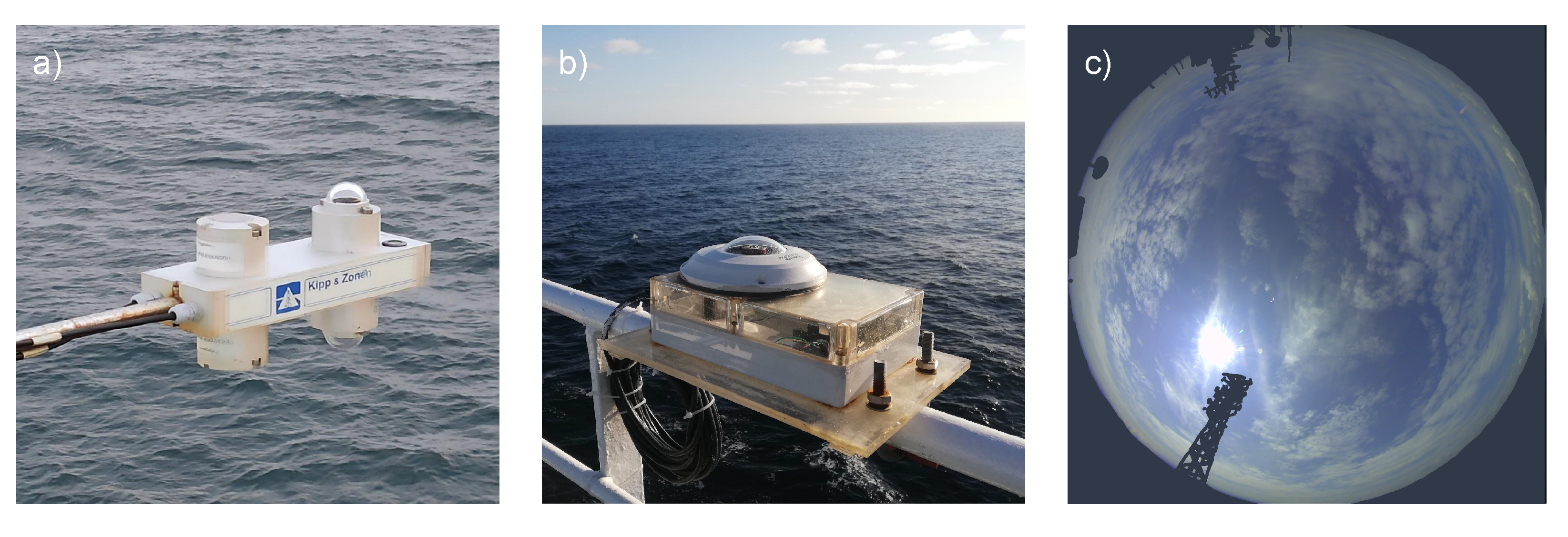
Figure 2.
Dataset target (SW radiation flux) distribution (histogram) and approximated cumulative density function (right panel). One may clearly see the imbalance of the dataset w.r.t. target value. We present the percentiles in the CDF figure using vertical red lines in order to demonstrate the inter-percentile distances.
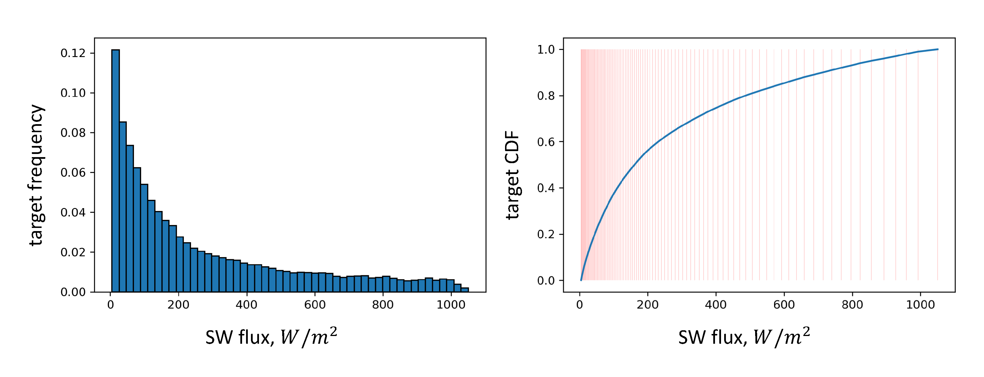
Figure 3.
Architecture of a CNN we exploited in our study. Here, with numbers, we present the shapes of input data or activation maps.
Figure 3.
Architecture of a CNN we exploited in our study. Here, with numbers, we present the shapes of input data or activation maps.
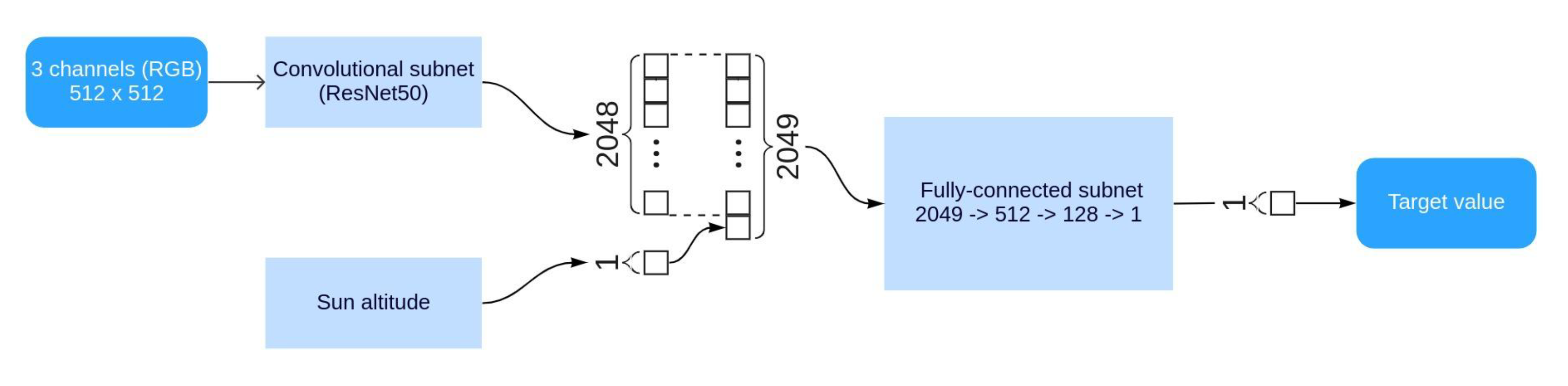
Figure 4.
Value mapping diagrams for: (a) Multilinear Regression as a baseline; (b) Random Forests without ITF re-weighting; (c) Random Forests using ITF re-weighting of train subset; (d) Gradient Boosting for Regression without ITF re-weighting; (e) Gradient Boosting for Regression using ITF re-weighting of train subset; (f) Convolutional neural network (no re-weighting). Here, density colormaps are logarithmic for presentation purpose.
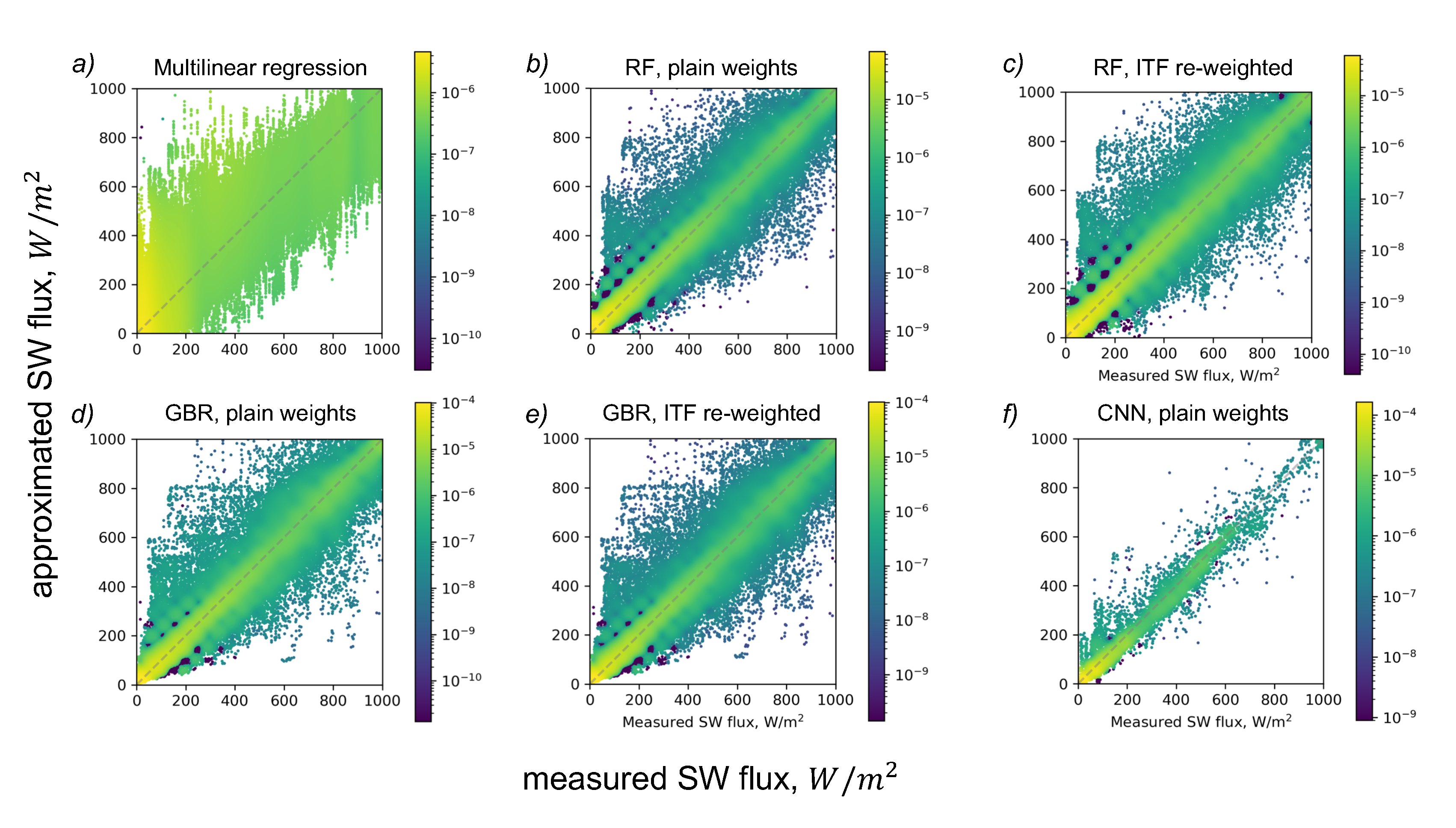
Figure 5.
Errors histograms for: (a) Multilinear Regression as a baseline; (b) Random Forests without ITF re-weighting; (c) Random Forests using ITF re-weighting of train subset; (d) Gradient Boosting for Regression without ITF re-weighting; (e) Gradient Boosting for Regression using ITF re-weighting of train subset; (f) Convolutional neural network (no re-weighting).
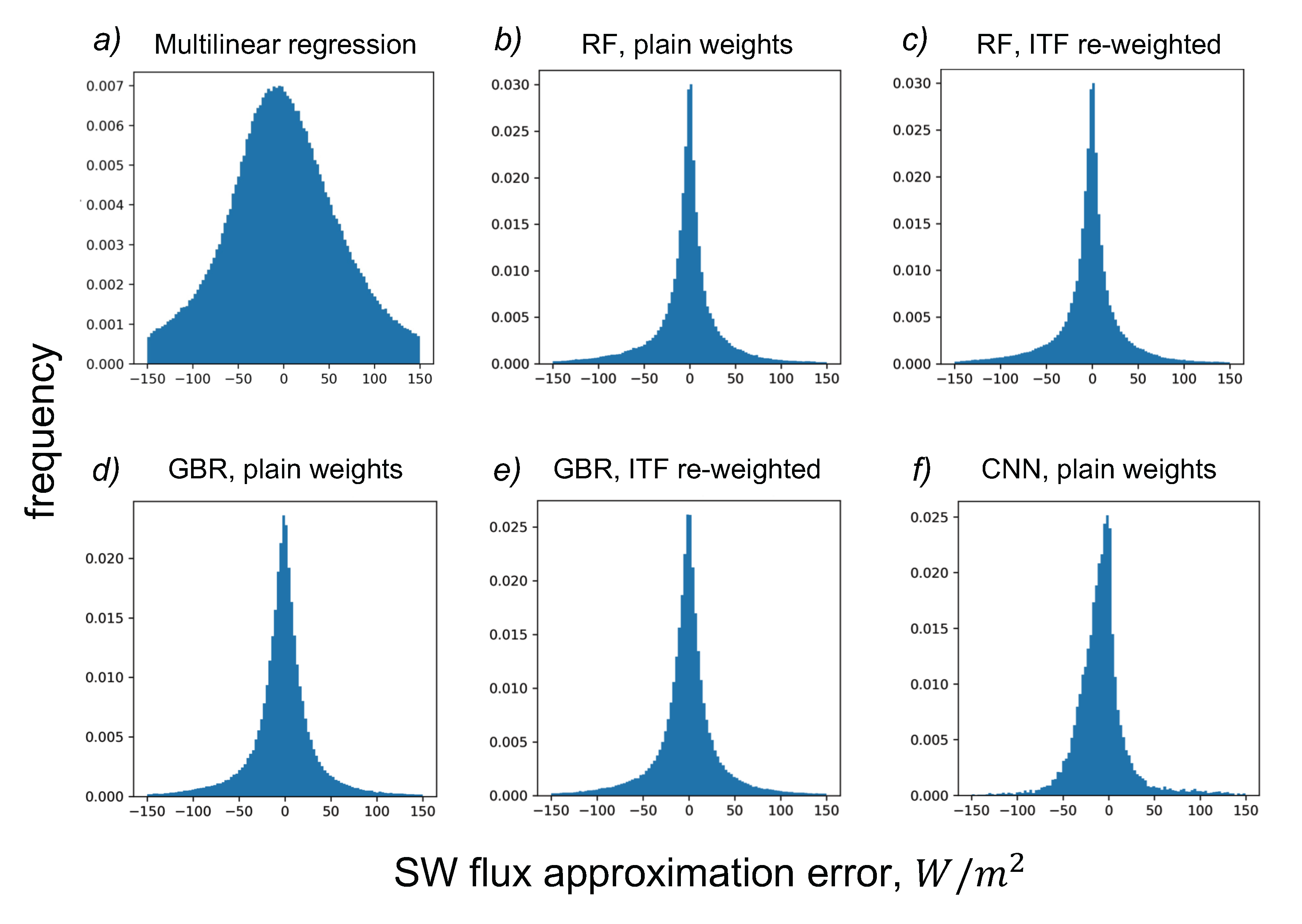

Table 1.
Summary for the dataset of our study.
| Subset | No. of objects |
| Train | 1 041 734 |
| Test | 350 859 |
| Total | 1 392 593 |
Table 2.
Quality metrics of (1-4) ML models used in this study and (5-6) parameterizations of SW radiation known from the literature.
Table 2.
Quality metrics of (1-4) ML models used in this study and (5-6) parameterizations of SW radiation known from the literature.
| No | Model | Parameterization | RMSE, |
|---|---|---|---|
| 1 | Multilinear Regression (baseline) | ||
| 2 | Random Forests, plain weights | ||
| 3 | Random Forests, ITF re-weighted | ||
| 4 | Gradient Boosting, plain weights | ||
| 5 | Gradient Boosting, ITF re-weighted | ||
| 4 | CNN | ||
| 5 | Dobson–Smith [34] | ||
| 6 | LVOAMKI [9] |
Disclaimer/Publisher’s Note: The statements, opinions and data contained in all publications are solely those of the individual author(s) and contributor(s) and not of MDPI and/or the editor(s). MDPI and/or the editor(s) disclaim responsibility for any injury to people or property resulting from any ideas, methods, instructions or products referred to in the content. |
© 2023 by the authors. Licensee MDPI, Basel, Switzerland. This article is an open access article distributed under the terms and conditions of the Creative Commons Attribution (CC BY) license (http://creativecommons.org/licenses/by/4.0/).
Copyright: This open access article is published under a Creative Commons CC BY 4.0 license, which permit the free download, distribution, and reuse, provided that the author and preprint are cited in any reuse.


