Submitted:
03 January 2023
Posted:
04 January 2023
You are already at the latest version
Abstract
This communication investigates possible anomalies in the lithosphere atmosphere and ionosphere on the occasion of the ML=3.3 earthquake that occurred on 1st January 2023 close to Guidonia Montecelio (Rome, Italy). This earthquake followed another event on 23 December 2022 of magnitude ML=3.1 with a very close epicentre (distance less than 1km). Seismological investigations clearly show an acceleration of seismicity in the last six months in the area. Two solutions of fitting time to failure power law on the Cumulative Benioff strain curve are the more likelihood: the ML3.3 of 1 January is the mainshock of seismic sequence or incoming earthquakes of a magnitude of about 4.1 provides a slightly better fit of the seismic data. Further investigation are necessary to assess if the accumulated stress have been totally released or not. No atmospheric anomalies related to this seismic activity have been identified even if some SO2 emissions could come from tectonic or volcanic sources in the South-Tyrrhenian Sea. Swarm satellites' magnetic data shows an anomalous track on 16 December 2022, which is temporally compatible with the seismic acceleration but other sources for the anomalous signal are also possible.
Keywords:
seismic acceleration
; Guidonia
; earthquake
; Benioff cumulative stress
; Swarm
; pre-earthquake processes
1. Introduction
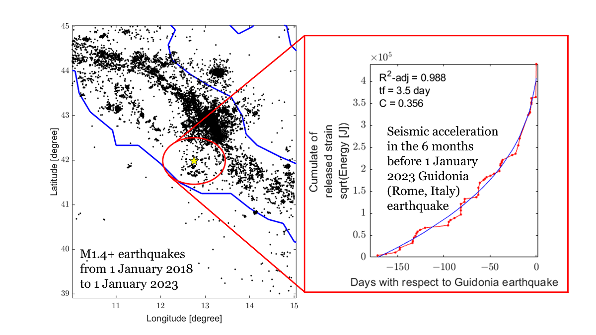
On 1 January 2023 at 13:07:46 Universal Time - UT (14:07 Italian time) an earthquake of magnitude ML=3.3 was localized by INGV North of the Capital of Italy, Rome. In particular the closest town is Guidonia Montecelio, and the epicenter was 3 km South-East from this town at the coordinates of 41.982° N and 12.750° E. The depth of earthquake was shallow with an hypocentral depth estimated equal to 9 km (http://cnt.rm.ingv.it/event/33781261, last access 2 January 2023). The event is relatively slow magnitude, but it got particular interest because it follows another seismic event with a slightly slower magnitude ML=3.1 occurred on 23 December 2022 at 16:35:13 UT (17:35 Italian time) with almost the same epicenter (41.984° N and 12.756° E, distance from the above cited event of about 0.5 km). The hypocentral depth of this event was estimated equal to 10 km (http://terremoti.ingv.it/event/33714971, last access 2 January 2023). Based on the data to INGV website at least 681 people (last update 1 January 2023 at 19:31 Italian time) felt the event on 23 December 2022 filling the form on https://www.hsit.it/ (last access 2 January 2023) and 765 people for the event on 1 January 2023 (last update 2 January 2023 at 3:55 Italian time). Previous earthquakes, around this event, were characterized by different focal mechanisms: toward North-East some thrust earthquakes have been historically recorded, while South-East normal fault and West side strike-slip. In particular, the Guidonia earthquakes that occurred on 23 December 2022 and 1 January 2023 could have been produced by a strike-slip fault proposed by Faccenna et al. [1] starting on Cornicolani Mounts and ending towards Colli Albani volcano district crossing Guidonia city (dashed line in Fig. 1 of their paper).
One basic question is if the events are part of a seismic sequence or a seismic swarm. The seismic sequence is characterized by a higher magnitude event (the mainshock) that is followed by aftershocks and could be preceded by foreshocks both of lower magnitude, while the seismic swarm is a chain of earthquakes of comparable and low magnitude without a clear mainshock [2]. If this is a seismic sequence it’s crucial to know if the event of magnitude ML=3.3 of 1 January 2023 is the mainshock or if a future event of higher magnitude is likely to occur. Furthermore, for seismic sequences the decay of the aftershocks generally follows the Omori-Utsu law [3], contrarywise, a seismic swarm has an almost constant seismic rate. The peculiarities of the seismic earthquakes of 22 December 2022 and 1 January 2023 localised close to Guidonia (Rome, Italy) motivates a further investigation that we report in this short communication, based on our previous experience of the lithosphere, atmosphere and ionosphere analysis prior to seismic events.
2. Materials and Methods
In this communication we investigated the earthquake catalogue, the atmospheric data from climatological archive and the Swarm satellites magnetic data.
2.1. Earthquake catalogue
The earthquake catalogue has been retrieved from INGV ISIDE [4] earthquake web portal (http://cnt.rm.ingv.it/, last access 2 January 2023) selecting the events inside the square box delimited by 41.5°N ≤ latitude ≤ 42.5°N and 12.2°E ≤ longitude ≤ 13.3°E from 1st January 2018 until 1st January 2023. No constrains have been selected for magnitude and depth, so all the events have been retrieved and they are 1253 earthquakes and their geographical localization is shown in Figure 1a. In the North-East corner of the map is visible some seismicity associate with the very long Italian Seismic Sequence of Amatrice-Norcia-Capitigliano (Montereale) 2016-2017 [5].
The completeness magnitude “Mc” has been analysed by the ZMap software [6] excluding the events of the above-cited Italian Seismic sequence (i.e., the event which are far more than 50 km from Guidonia 2023 earthquake) to avoid a bias in the analysis. In fact, the Apennines central region of Italy interested by the sequence could be better covered not only with permanent seismic stations but also for temporary stations installed after the start of the same sequence. Completeness magnitude was found equal to Mc = 1.4 as visible in graph in Figure 1b. In the following analyses only the earthquakes with magnitude M ≥ Mc will be taken into account. The cumulative Benioff stress has been computed for the events inside the Dobrovoslky radius. Benioff stress in an indication of the stress that is accumulating on a fault [7]. The Dobrovoslky radius is the distance typically used to estimate the preparation area of an earthquake [8].
In particular, Dobrovolsky radius in kilometres is
The Benioff cumulative stress S(t) is
where “i” is the th-earthquake with magnitude Mi and N(t) is the total number of earthquakes occurred until the time t. According to Mignan et al. [9] and Cianchini et al. [10] the following time-to-failure power law has been fitted to the Benioff cumulative stress:
where A and B parameters are proportional to the initial and final accumulated stress and m is an exponential factor in the range from 0 to 1 and it is typically equal to 0.3 [10]. In this work, m has been fixed to m=3 to guaranty stability of the power law fit. The graphs report tf which is the time to failure, i.e., the likelihood estimation of the mainshock time.
2.2. Atmospheric data processing
To investigate the atmospheric proprieties the data from the climatological archive MERRA-2 by NASA [11] have been investigated. With the experience of previous investigated earthquake, the MEANS software has been used with the remotion of a linear trend to take into account the possible effect of the global warming as done in De Santis et al. [12] for Ridgecrest, US, 2019 earthquake analysis. The MEANS algorithm has been used the first time by Piscini et al. [13] to investigate volcano eruptions and after applied to several other volcano eruptions and earthquakes [12,14,15,16,17,18]. The algorithm essentially estimates the typical value of the atmospheric parameter for the day and region constructing an historical time series and in particular the mean and standard deviation of the parameter for the area under study. If the parameter in the year with the natural hazard event overpasses two standard deviations of the historical time series is defined as anomalous. In this report we investigated surface air temperature, aerosol and Sulphur dioxide.
2.3. Ionospheric data processing
The ionosphere has been monitored by the European Space Agency (ESA) Swarm constellation. Swarm mission is composed by three identical satellites in low Earth quasi-polar orbits, called Alpha, Bravo and Charlie aiming to measure the geomagnetic field with the best precision available at the state of art [19]. The use of Swarm data to study the preparation of the earthquakes has been explored by several researches in the last years using a single case study approach [18,20,21,22,23,24,25,26,27,28,29,30,31] or even statistically correlating the magnetic and electron density anomalies of Swarm with M5.5+ earthquakes occurred in the first 4.7 years of Swarm mission by De Santis et al. [32], the first 8 years by Marchetti et al. [33] or using Machine Learning by Xiong et al. [34].
In this report we applied the MASS algorithm to Swarm magnetic field data defined with all details in [27,31,32,33]. It analyses the data track by track removing the background with estimating the derivative and subtracting a cubic spline. The residuals are monitored by a moving window and comparing the root mean square of the window with the one of the entire track among −50°S and +50°N of geomagnetic latitude to avoid the influence of polar activity.
3. Results
Here we illustrate the results for seismological atmospheric and ionospheric investigations in respectively sections.
3.1. Seismological investigation
The cumulative Benioff stress has been calculated inside the Dobrovoslky area testing several mainshocks from magnitude 3.3 until 5.5 as listed in Table 1. The lower limit corresponds to the assumption that the event of 1 January 2023 would be the mainshock and the higher magnitude events correspond to the hypothesis that a higher magnitude event is incoming. In case the Dobrovolsky radius overpassed the area represented in Figure 1a, the earthquake with M ≥ Mc have been further retrieved.
For each fit the adjusted R2 and the estimated time of failure is reported in Figure 2, Figure 3 and Figure 4 for 5 years, 1 year and 6 months before the ML=3.3, 1 January 2023 Guidonia earthquake, respectively.
In addition the acceleration coefficient C defined by Cianchini et al. [10] has been reported calculating as:
As much as low is “C” as much the fit represents an acceleration, on the other hand C = 1 indicates that the trend is linear or C > 1 that linear fit is better than power law. Such situation could be due to a trend which is influenced by aftershock of another seismic sequence as the one of Amatrice-Norcia-Capitigliano (Montereale) Central Italy 2016-2017, in particular for long trend and larger radius of analysis.
The investigations in 5 years and 1 year before ML=3.3 Guidonia 1st January 2023 earthquake don’t provide interesting results. In fact, the trends are dominated by other important seismicity which occurred in the area (for example Mw=3.3 11 April 2022, Ciciliano, Rome event http://cnt.rm.ingv.it/event/30543871, last access 2 January 2023). The tests with larger magnitude are instead dominated by the residual sequence of Apennine cited above. This is the reason why higher magnitude than 4.7 are not reliable to be tested as the crossing with seismicity from Central Apennines region becomes predominant.
On the other hand, the investigation in the 6 months before ML=3.3 Guidonia 1st January 2023 earthquake reported in Figure 4, provide interesting results. From magnitude 3.3 until 3.9 the estimated time-to-failure is 0.0 days and the maximum acceleration is reported for M=3.3 with C=0.318. Considering that no higher events have been recorded in this area at 1 January 2023, among these 4 analyses the most reliable need to be considered the test in M=3.3, i.e., the hypothesis that the past earthquake was the mainshock. Despite this, the analysis for M=4.1 and M=4.3 provided good fits with a time to failure in few days (M4.1 on 5 January 2023 or M4.3 on 25 February 2023). The investigations of M4.5 and 4.7 provided very goodness of the fits even though they are almost linear (as underlined by their C close to 1). So, selecting the analysis with higher adjusted R2 and the most reliable result is the analysis of M4.1 with a time to failure in 3.5 days after Guidonia 1st January 2023 earthquake with R2-adj = 0.988 and C = 0.356. Even though this could appear as a prediction, that interpretation is not totally correct, in fact, firstly it’s necessary to estimate the maximum magnitude that the interested fault could generate, and secondary determine if the accumulated stress has been totally or partially released by these events. Furthermore, the time-to-failure power law could not take into account several geological and tectonic factors, so it cannot be used “alone”. Finally, the right interpretation for the authors is that in the past six months in the circle area of radius 58km centered on Guidonia 1 January 2023 earthquake has been recorded a clear seismic acceleration, but further studies are necessary to propose eventual future scenarios.
3.2. Atmospheric investigations
In this section we presented atmospheric investigation in the six months before Guidonia 1st January 2023 earthquake. The time series ends on 30 November due to December data still not yet available. The results of surface air temperature, aerosol and SO2 are provided in Supplementary Materials in Figure S1, S2 and S3 respectively. All the time series were calculated in a square box centered on the Guidonia 1st January 2023 earthquake with 3° side. Surface air temperature have some anomalous values but no-one of them have a persistence which is a criteria that was found effective for Central Italy by Piscini et al. [35]. Nevertheless, aerosol and especially SO2 provided several anomalous days and we provided here their geographical map to investigate better if the increase of these quantities is local or global. The aerosol on 18 August 2022 is particularly anomalous and its map is shown in Figure 5. From the distribution of the aerosol, it seems that all the Tyrrhenian Sea recorded high value of aerosol, probably due to some special weather conditions and in any case, it doesn’t seem related to the earthquake.
Figure 6 reported 3 anomalous days of SO2 in the investigated area, i.e., the 18 July, 23 October and 1 November 2022. The 18 July and 1 November show a slightly higher value of SO2 almost on all the coastline, excluding a local phenomenon. Despite this in all the 3 maps the highest values are recorded in the sea in correspondence of an important subduction slab of Tyrrhenian Sea (dashed grey line). The mechanism of emission of this SO2 could be due to the stress on the subduction place, but also to the important volcanic activity for the several volcanos close to this area (Aeolian Islands with Stromboli, submersed Marsili, or Etna slightly southern in Sicily). These volcanos are not only well known to emit SO2 but also they contributed significantly to the global budget of SO2 emissions [36].
3.3. Ionospheric Investigations
The ionosphere has been investigated under the most reliable seismological results of an earthquake of M4.1 and so with the corresponding Dobrovolsky’s area. MASS algorithm has been run for the data from 3 July 2022 until 28 December 2022 (last available data with standard Swarm processor of MAGX_LR data product).
Considering the very low dimension of the research area, Swarm satellites do not cross all days within the area, reducing the chances to detect possible electromagnetic signals. After processing all the tracks of Swarm Alpha, Bravo and Charlie, only 4 tracks present some anomalies inside the research area in geomagnetic quiet conditions (|Dst| ≤ 20 nT and ap ≤ 10 nT), using a window of 1° latitude (found optimal in Central Italy Swarm investigation [37]) and a threshold of rms inside the window to be more than 2.5 times the one of the whole track. Table 2 reports the list of anomalous tracks. No anomalies have been identified in vertical Z component or in absolute scalar intensity of geomagnetic field with the selected parameters.
The most two interesting tracks in Y-East component of geomagnetic field are reported in Figure 7 and 8 and the other two anomalous tracks in Figure S4 and S5 of Supplementary Materials. In particular, Figure 7 shows an anomalous signal of about 3 nT/s peak-peak intensity, but the geomagnetic index Dst is at the upper boundary limit of 20 nT. In fact, looking at the trend of Dst (e.g., on https://wdc.kugi.kyoto-u.ac.jp/dst_realtime/202208/index.html, last access 2 January 2023) it continuous to increase in the following hours and after decreasing reaching −58 nT on 8 August 2022, so this track was acquired in the Sudden Commencement of a very moderate geomagnetic storm. Despite the signal is perfectly center on the incoming earthquake the external source is the more reliable one.
Figure 8 shows instead a track of Swarm Bravo acquired during very quiet geomagnetic conditions (Dst = −1 nT, ap = 2 nT) with an anomalous geomagnetic field Y-East component signal recorded above Central Italy. Despite the track preceded the first shock of ML3.1 of 23 December 2022 of one week and during the seismic acceleration phase the diffuse nature of the anomaly seems difficult to confirm it could be seismo-induced even it cannot be excluded.
4. Discussion and conclusions
In this Communication paper we investigated the ML=3.3 Guidonia (Rome, Italy) earthquake occurred on 1 January 2023 by seismic catalogue, atmospheric and ionospheric data. From a preliminary investigation, a seismological analysis identified an acceleration of the seismicity around such epicenter especially focusing in the last six months. The atmospheric and ionospheric investigations, on the other hand, don’t provide any results which look as seismo-induced nature. The absence of possible coupling of the lithosphere with atmosphere and ionosphere is in agreement with the low magnitude of the seismic event (ML=3.3).
Finally, the seismological investigation suggest that these events are likely part of a seismic sequence and the analysis are compatible with 2 main hypotheses:
- The ML3.3 of 1 January 2023 is the mainshock of the seismic quiescence (R2-adj = 0.977 and acceleration coefficient C = 0.32)
- The mainshock could be an incoming event of magnitude M4.1 (R2-adj = 0.988 and acceleration coefficient C = 0.36).
The second hypothesis seems mathematically slightly more probable, but both the hypotheses describe well the seismicity recorded in the last months around Guidonia (Rome, Italy). In any case, the acceleration nature (C << 1) of all the reliable solutions tend to exclude that the events are part of a seismic swarm.
Even though some speculation on the evolution of the seismic activity can be done, they cannot be considered as a prediction, because no tests have been ever made, so without a validation of the method by an independent organism (e.g., CSEP, https://cseptesting.org/, last access 2 January 2023) the analysis has no prediction value. Furthermore, the correct interpretation of the time-to-failure power law fit is that in the last six months in a circle area of radius of about 58 km has been detected a seismic acceleration but to propose future evolution of the seismic sequence further investigations are absolutely necessary. Due to the peculiarity observed in the past months it could be evaluated the installation of geochemical multi-parametric station to detect eventual gases or fluids released from the ground.
Finally, this example, shows how these techniques could be applied in real time for monitoring (not yet prediction) purpose of lithosphere, atmosphere and ionosphere and the help of remote sensing data to understand and monitor our vulnerable planet.
Author Contributions
Conceptualization, methodology, software, writing—original draft preparation, formal analysis, investigation, data curation, visualization, D.M.; supervision Z.K.; validation L.M.; resources, project administration, funding acquisition, Z.K. and D.M; writing—review and editing L.M., D.M., Z.Y., K.Z., W.C., Y.C., M.F., T.W., S.W., J.W., D.Z. and H.Z. All authors have read and agreed to the published version of the manuscript.
Funding
This research was funded by the National Natural Science Foundation of China, grant number 41974084; the China Postdoctoral Science Foundation, grant number 2021M691190; the International Cooperation Project of the Department of Science and Technology of Jilin Province, grant number 20200801036GH.
Data Availability Statement
We acknowledge the INGV for the seismic catalogue used in this paper, freely available at http://cnt.rm.ingv.it/, last access 3 January 2023. MERRA-2 data can be downloaded from https://disc.gsfc.nasa.gov/datasets?project=MERRA-2 (last access on 2 January 2023) with Earth Observation NASA free credential. Swarm data are freely available via ftp and http at swarm-diss.eo.esa.int server (last access on 2 January 2023).
Acknowledgments
We would acknowledge Alessandro Piscini, Rita Di Giovambattista, Gianfranco Cianchini, Francisco Javier Pavón-Carrasco, Saioa Arquero Campuzano, Dario Sabbagh, Loredana Perrone, Maurizio Soldani and Angelo De Santis for their contributions in the preparation, writing and optimisation of some codes re-used in this work originally developed for some of the cited papers and constructive scientific discussion on previous work whose concepts are here re-applied.
Conflicts of Interest
The authors declare no conflict of interest. The funders had no role in the design of the study; in the collection, analyses, or interpretation of data; in the writing of the manuscript; or in the decision to publish the results.
References
- Faccenna, C.; Soligo, M.; Billi, A.; De Filippis, L.; Funiciello, R.; Rossetti, C.; Tuccimei, P. Late Pleistocene Depositional Cycles of the Lapis Tiburtinus Travertine (Tivoli, Central Italy): Possible Influence of Climate and Fault Activity. Global and Planetary Change 2008, 63, 299–308. [Google Scholar] [CrossRef]
- Frepoli, A.; Cimini, G.B.; De Gori, P.; De Luca, G.; Marchetti, A.; Monna, S.; Montuori, C.; Pagliuca, N.M. Seismic Sequences and Swarms in the Latium-Abruzzo-Molise Apennines (Central Italy): New Observations and Analysis from a Dense Monitoring of the Recent Activity. Tectonophysics 2017, 712–713, 312–329. [Google Scholar] [CrossRef]
- Utsu, T.; Ogata, Y.; S, R.; Matsu’ura The Centenary of the Omori Formula for a Decay Law of Aftershock Activity. J,Phys,Earth 1995, 43, 1–33. [CrossRef]
- ISIDe Working Group Italian Seismological Instrumental and Parametric Database (ISIDe). 2007. [CrossRef]
- Chiaraluce, L.; Di Stefano, R.; Tinti, E.; Scognamiglio, L.; Michele, M.; Casarotti, E.; Cattaneo, M.; De Gori, P.; Chiarabba, C.; Monachesi, G.; et al. The 2016 Central Italy Seismic Sequence: A First Look at the Mainshocks, Aftershocks, and Source Models. Seismological Research Letters 2017, 88, 757–771. [Google Scholar] [CrossRef]
- Wiemer, S. A Software Package to Analyze Seismicity: ZMAP. Seismological Research Letters 2001, 72, 373–382. [Google Scholar] [CrossRef]
- Mignan, A. The Stress Accumulation Model: Accelerating Moment Release and Seismic Hazard. In Advances in Geophysics; Elsevier, 2008; Vol. 49, pp. 67–201 ISBN 978-0-12-374231-5.
- Dobrovolsky, I.P.; Zubkov, S.I.; Miachkin, V.I. Estimation of the Size of Earthquake Preparation Zones. PAGEOPH 1979, 117, 1025–1044. [Google Scholar] [CrossRef]
- Mignan, A.; King, G.C.P.; Bowman, D. A Mathematical Formulation of Accelerating Moment Release Based on the Stress Accumulation Model. J. Geophys. Res. 2007, 112, B07308. [Google Scholar] [CrossRef]
- Cianchini, G.; De Santis, A.; Di Giovambattista, R.; Abbattista, C.; Amoruso, L.; Campuzano, S.A.; Carbone, M.; Cesaroni, C.; De Santis, A.; Marchetti, D.; et al. Revised Accelerated Moment Release Under Test: Fourteen Worldwide Real Case Studies in 2014–2018 and Simulations. Pure Appl. Geophys. 2020, 177, 4057–4087. [Google Scholar] [CrossRef]
- Gelaro, R.; McCarty, W.; Suárez, M.J.; Todling, R.; Molod, A.; Takacs, L.; Randles, C.A.; Darmenov, A.; Bosilovich, M.G.; Reichle, R.; et al. The Modern-Era Retrospective Analysis for Research and Applications, Version 2 (MERRA-2). J. Climate 2017, 30, 5419–5454. [Google Scholar] [CrossRef] [PubMed]
- De Santis, A.; Cianchini, G.; Marchetti, D.; Piscini, A.; Sabbagh, D.; Perrone, L.; Campuzano, S.A.; Inan, S. A Multiparametric Approach to Study the Preparation Phase of the 2019 M7.1 Ridgecrest (California, United States) Earthquake. Front. Earth Sci. 2020, 8, 540398. [Google Scholar] [CrossRef]
- Piscini, A.; Marchetti, D.; De Santis, A. Multi-Parametric Climatological Analysis Associated with Global Significant Volcanic Eruptions During 2002–2017. Pure Appl. Geophys. 2019, 176, 3629–3647. [Google Scholar] [CrossRef]
- Marchetti, D.; De Santis, A.; D’Arcangelo, S.; Poggio, F.; Piscini, A.; A. Campuzano, S.; De Carvalho, W.V.J.O. Pre-Earthquake Chain Processes Detected from Ground to Satellite Altitude in Preparation of the 2016–2017 Seismic Sequence in Central Italy. Remote Sensing of Environment 2019, 229, 93–99. [CrossRef]
- Marchetti, D.; Zhu, K.; Zhang, H.; Zhima, Z.; Yan, R.; Shen, X.; Chen, W.; Cheng, Y.; He, X.; Wang, T.; et al. Clues of Lithosphere, Atmosphere and Ionosphere Variations Possibly Related to the Preparation of La Palma 19 September 2021 Volcano Eruption. Remote Sensing 2022, 14, 5001. [Google Scholar] [CrossRef]
- Akhoondzadeh, M.; De Santis, A.; Marchetti, D.; Wang, T. Developing a Deep Learning-Based Detector of Magnetic, Ne, Te and TEC Anomalies from Swarm Satellites: The Case of Mw 7.1 2021 Japan Earthquake. Remote Sensing 2022, 14, 1582. [Google Scholar] [CrossRef]
- Akhoondzadeh, M.; Marchetti, D. Developing a Fuzzy Inference System Based on Multi-Sensor Data to Predict Powerful Earthquake Parameters. Remote Sensing 2022, 14, 3203. [Google Scholar] [CrossRef]
- Marchetti, D.; De Santis, A.; Shen, X.; Campuzano, S.A.; Perrone, L.; Piscini, A.; Di Giovambattista, R.; Jin, S.; Ippolito, A.; Cianchini, G.; et al. Possible Lithosphere-Atmosphere-Ionosphere Coupling Effects Prior to the 2018 Mw = 7.5 Indonesia Earthquake from Seismic, Atmospheric and Ionospheric Data. Journal of Asian Earth Sciences 2020, 188, 104097. [Google Scholar] [CrossRef]
- Friis-Christensen, E.; Lühr, H.; Hulot, G. Swarm: A Constellation to Study the Earth’s Magnetic Field. Earth Planet Sp 2006, 58, 351–358. [Google Scholar] [CrossRef]
- Akhoondzadeh, M.; De Santis, A.; Marchetti, D.; Piscini, A.; Cianchini, G. Multi Precursors Analysis Associated with the Powerful Ecuador (MW= 7.8) Earthquake of 16 April 2016 Using Swarm Satellites Data in Conjunction with Other Multi-Platform Satellite and Ground Data. Advances in Space Research 2018, 61, 248–263. [Google Scholar] [CrossRef]
- Zhu, K.; Li, K.; Fan, M.; Chi, C.; Yu, Z. Precursor Analysis Associated With the Ecuador Earthquake Using Swarm A and C Satellite Magnetic Data Based on PCA. IEEE Access 2019, 7, 93927–93936. [Google Scholar] [CrossRef]
- Zhu, K.; Fan, M.; He, X.; Marchetti, D.; Li, K.; Yu, Z.; Chi, C.; Sun, H.; Cheng, Y. Analysis of Swarm Satellite Magnetic Field Data Before the 2016 Ecuador (Mw = 7.8) Earthquake Based on Non-Negative Matrix Factorization. Front. Earth Sci. 2021, 9, 621976. [Google Scholar] [CrossRef]
- Fan, M.; Zhu, K.; De Santis, A.; Marchetti, D.; Cianchini, G.; Piscini, A.; He, X.; Wen, J.; Wang, T.; Zhang, Y.; et al. Analysis of Swarm Satellite Magnetic Field Data for the 2015 Mw 7.8 Nepal Earthquake Based on Nonnegative Tensor Decomposition. IEEE Trans. Geosci. Remote Sensing 2022, 60, 1–19. [Google Scholar] [CrossRef]
- Ghamry, E.; Mohamed, E.K.; Sekertekin, A.; Fathy, A. Integration of Multiple Earthquakes Precursors before Large Earthquakes: A Case Study of 25 April 2015 in Nepal. Journal of Atmospheric and Solar-Terrestrial Physics 2023, 242, 105982. [Google Scholar] [CrossRef]
- Marchetti, D.; De Santis, A.; Campuzano, S.A.; Soldani, M.; Piscini, A.; Sabbagh, D.; Cianchini, G.; Perrone, L.; Orlando, M. Swarm Satellite Magnetic Field Data Analysis Prior to 2019 Mw = 7.1 Ridgecrest (California, USA) Earthquake. Geosciences 2020, 10, 502. [Google Scholar] [CrossRef]
- De Santis, A.; Perrone, L.; Calcara, M.; Campuzano, Saioa., A.; Cianchini, G.; D’Arcangelo, S.; Di Mauro, D.; Marchetti, D.; Nardi, A.; Orlando, M.; et al. A Comprehensive Multiparametric and Multilayer Approach to Study the Preparation Phase of Large Earthquakes from Ground to Space: The Case Study of the June 15 2019, M7.2 Kermadec Islands (New Zealand) Earthquake. Remote Sensing of Environment 2022, 283, 113325. [CrossRef]
- De Santis, A.; Marchetti, D.; Spogli, L.; Cianchini, G.; Pavón-Carrasco, F.J.; Franceschi, G.D.; Di Giovambattista, R.; Perrone, L.; Qamili, E.; Cesaroni, C.; et al. Magnetic Field and Electron Density Data Analysis from Swarm Satellites Searching for Ionospheric Effects by Great Earthquakes: 12 Case Studies from 2014 to 2016. Atmosphere 2019, 10, 371. [Google Scholar] [CrossRef]
- Marchetti, D.; Akhoondzadeh, M. Analysis of Swarm Satellites Data Showing Seismo-Ionospheric Anomalies around the Time of the Strong Mexico (Mw = 8.2) Earthquake of 08 September 2017. Advances in Space Research 2018, 62, 614–623. [Google Scholar] [CrossRef]
- Akhoondzadeh, M.; De Santis, A.; Marchetti, D.; Shen, X. Swarm-TEC Satellite Measurements as a Potential Earthquake Precursor Together With Other Swarm and CSES Data: The Case of Mw7.6 2019 Papua New Guinea Seismic Event. Front. Earth Sci. 2022, 10, 820189. [Google Scholar] [CrossRef]
- Christodoulou, V.; Bi, Y.; Wilkie, G. A Tool for Swarm Satellite Data Analysis and Anomaly Detection. PLoS ONE 2019, 14, e0212098. [Google Scholar] [CrossRef] [PubMed]
- De Santis, A.; Balasis, G.; Pavón-Carrasco, F.J.; Cianchini, G.; Mandea, M. Potential Earthquake Precursory Pattern from Space: The 2015 Nepal Event as Seen by Magnetic Swarm Satellites. Earth and Planetary Science Letters 2017, 461, 119–126. [Google Scholar] [CrossRef]
- De Santis, A.; Marchetti, D.; Pavón-Carrasco, F.J.; Cianchini, G.; Perrone, L.; Abbattista, C.; Alfonsi, L.; Amoruso, L.; Campuzano, S.A.; Carbone, M.; et al. Precursory Worldwide Signatures of Earthquake Occurrences on Swarm Satellite Data. Sci Rep 2019, 9, 20287. [Google Scholar] [CrossRef] [PubMed]
- Marchetti, D.; De Santis, A.; Campuzano, S.A.; Zhu, K.; Soldani, M.; D’Arcangelo, S.; Orlando, M.; Wang, T.; Cianchini, G.; Di Mauro, D.; et al. Worldwide Statistical Correlation of Eight Years of Swarm Satellite Data with M5.5+ Earthquakes: New Hints about the Preseismic Phenomena from Space. Remote Sensing 2022, 14, 2649. [Google Scholar] [CrossRef]
- Xiong, P.; Marchetti, D.; De Santis, A.; Zhang, X.; Shen, X. SafeNet: SwArm for Earthquake Perturbations Identification Using Deep Learning Networks. Remote Sensing 2021, 13, 5033. [Google Scholar] [CrossRef]
- Piscini, A.; De Santis, A.; Marchetti, D.; Cianchini, G. A Multi-Parametric Climatological Approach to Study the 2016 Amatrice–Norcia (Central Italy) Earthquake Preparatory Phase. Pure Appl. Geophys. 2017, 174, 3673–3688. [Google Scholar] [CrossRef]
- Allard, P.; Carbonnelle, J.; Métrich, N.; Loyer, H.; Zettwoog, P. Sulphur Output and Magma Degassing Budget of Stromboli Volcano. Nature 1994, 368, 326–330. [Google Scholar] [CrossRef]
- Marchetti, D.; De Santis, A.; D’Arcangelo, S.; Poggio, F.; Jin, S.; Piscini, A.; Campuzano, S.A. Magnetic Field and Electron Density Anomalies from Swarm Satellites Preceding the Major Earthquakes of the 2016–2017 Amatrice-Norcia (Central Italy) Seismic Sequence. Pure Appl. Geophys. 2020, 177, 305–319. [Google Scholar] [CrossRef]
Figure 1.
Earthquakes occurred around Guidonia (Rome) from 1st January 2018 until 1st January 2023. (a) Geographical map of the events with yellow stars for the event with magnitude M ≥ 3; (b) Gutenberg-Richter distributions of the magnitude of the earthquakes excluding the seismicity in the North-East corner of the map, i.e., within a radius of 50 km from Guidonia epicenters.
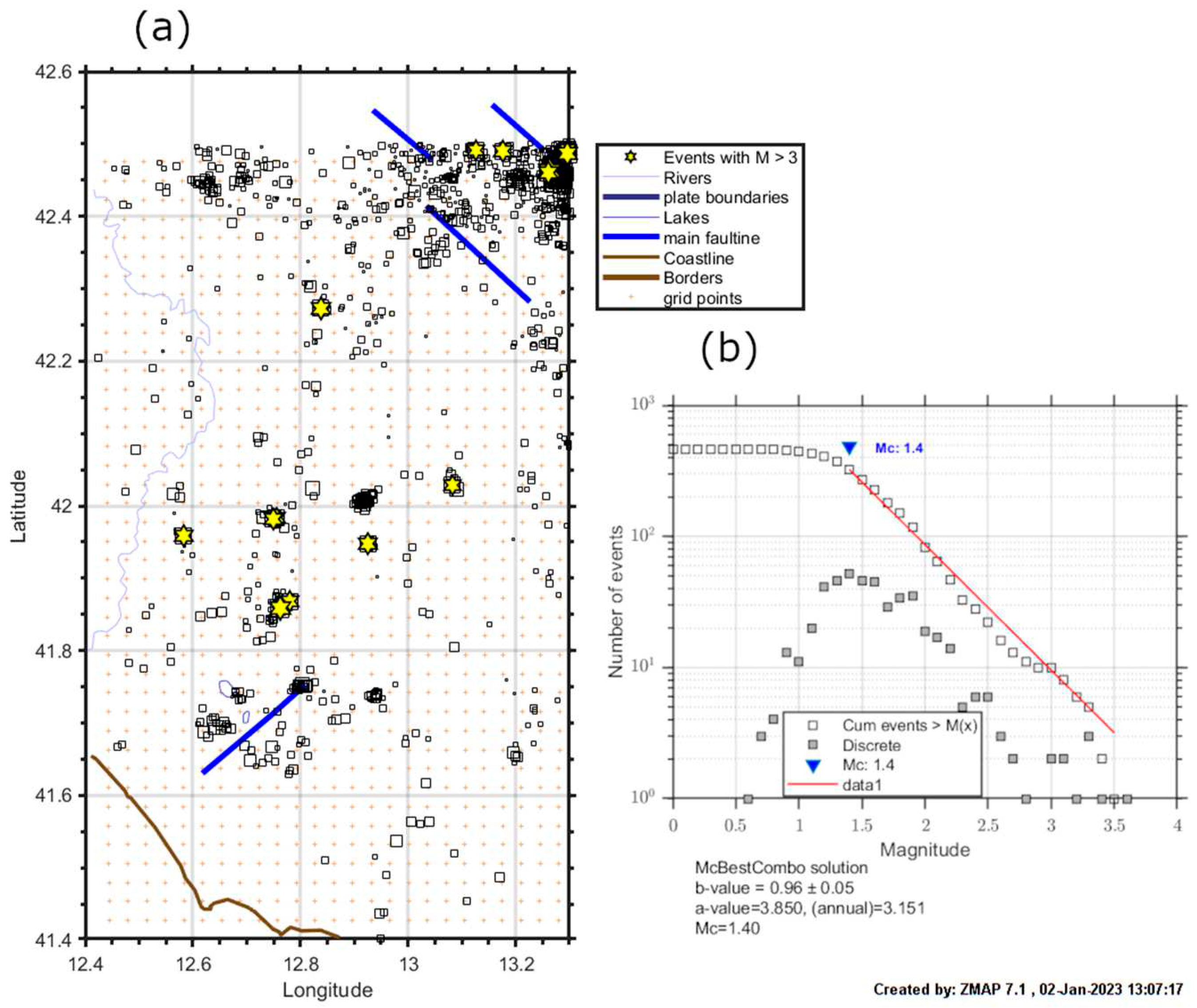
Figure 2.
Benioff cumulative stress curves in the 5 years before the ML=3.3 1 January 2023 Guidonia earthquake tested in the Dobrovolsky areas of earthquakes with magnitude from 3.3 to 4.7. For each plot the blue curve represents the time-to-failure power law fit, whose R2-adg. and tf are reported. The acceleration coefficient C is also reported.
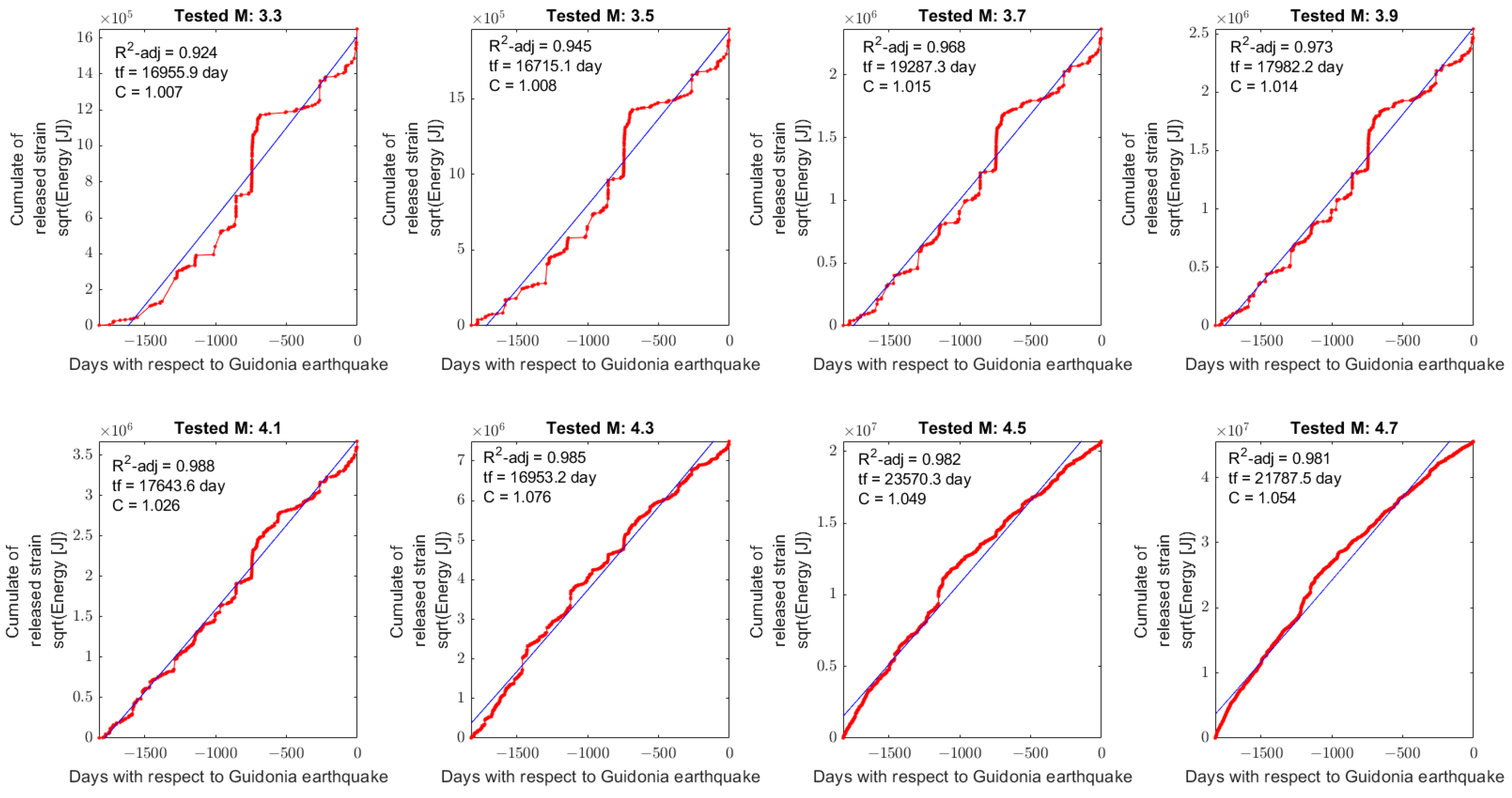
Figure 3.
The same as Figure 2, but calculated in one year before the ML=3.3 1 January 2023 Guidonia earthquake.
Figure 3.
The same as Figure 2, but calculated in one year before the ML=3.3 1 January 2023 Guidonia earthquake.
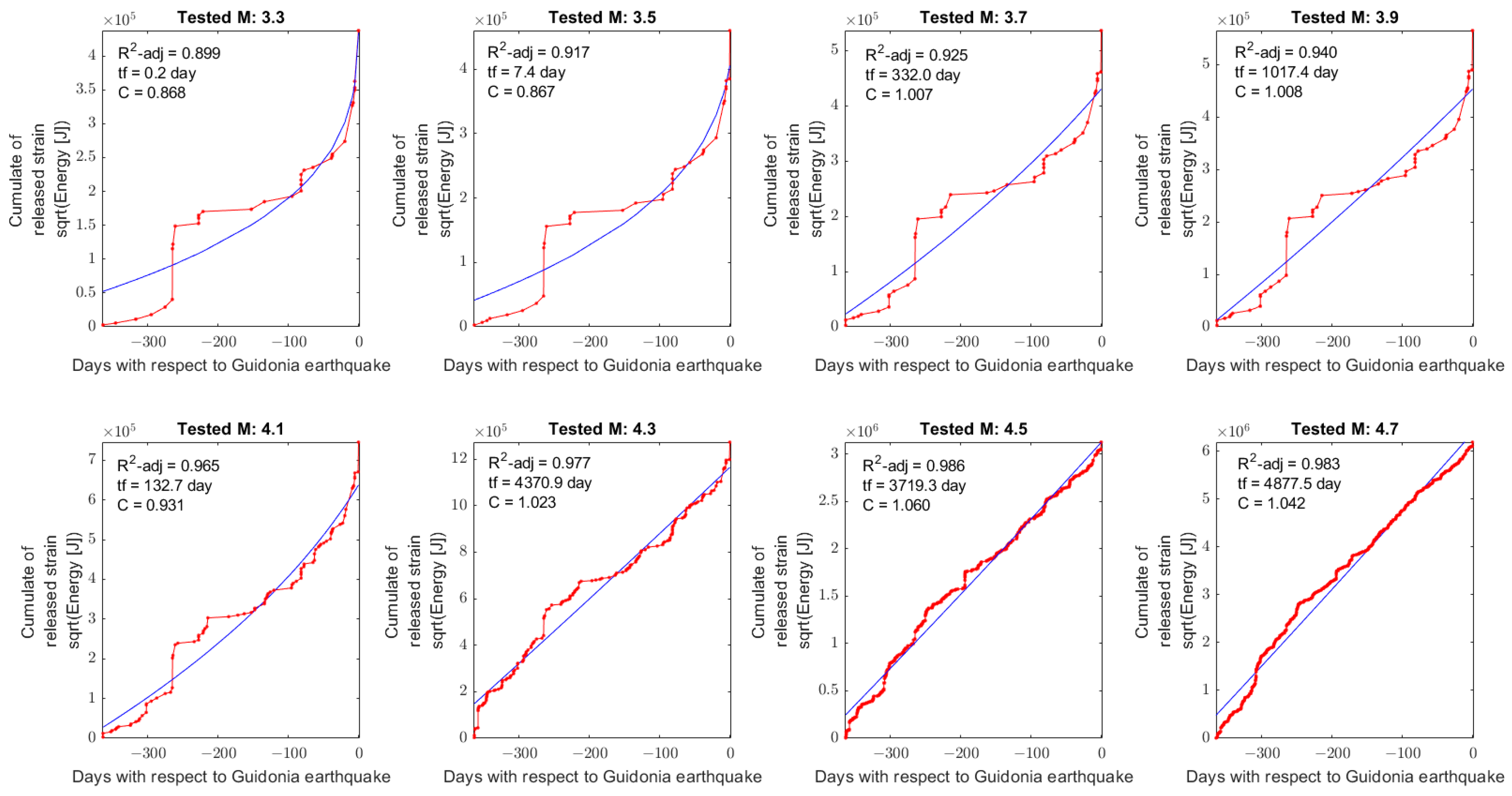
Figure 4.
The same as Figure 2, but calculated in six months before the ML=3.3 1 January 2023 Guidonia earthquake.
Figure 4.
The same as Figure 2, but calculated in six months before the ML=3.3 1 January 2023 Guidonia earthquake.
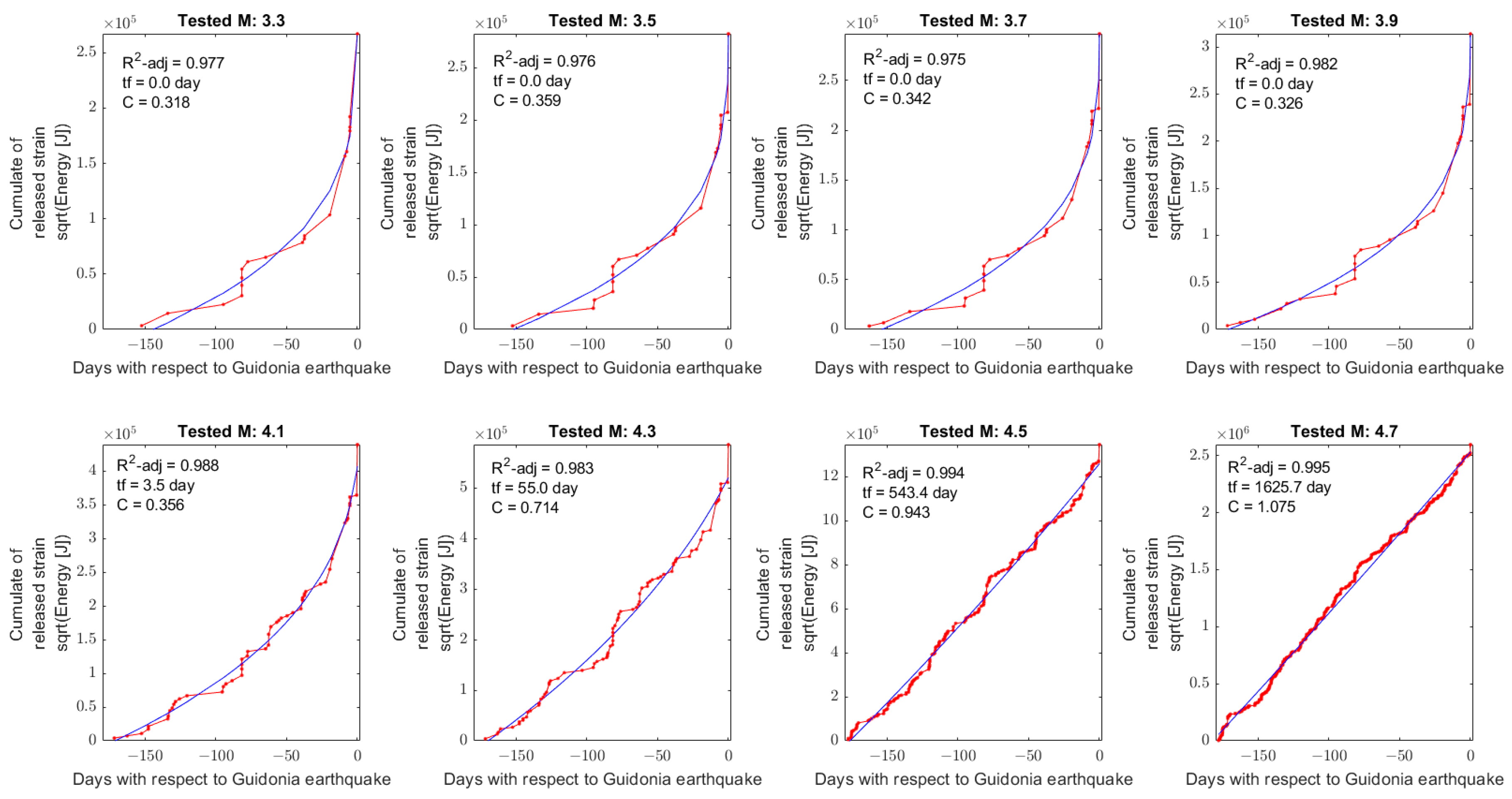
Figure 5.
Aerosol map on the 18 August 2022. The epicenter of Guidonia 1 January 2023 earthquake is shown with a white star.
Figure 5.
Aerosol map on the 18 August 2022. The epicenter of Guidonia 1 January 2023 earthquake is shown with a white star.
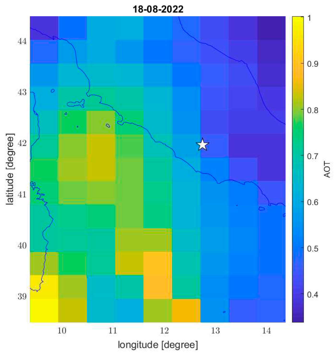
Figure 6.
SO2 maps on 17 July, 23 October and 1 November 2022. The epicenter of Guidonia 1 January 2023 earthquake is shown with a white star.
Figure 6.
SO2 maps on 17 July, 23 October and 1 November 2022. The epicenter of Guidonia 1 January 2023 earthquake is shown with a white star.
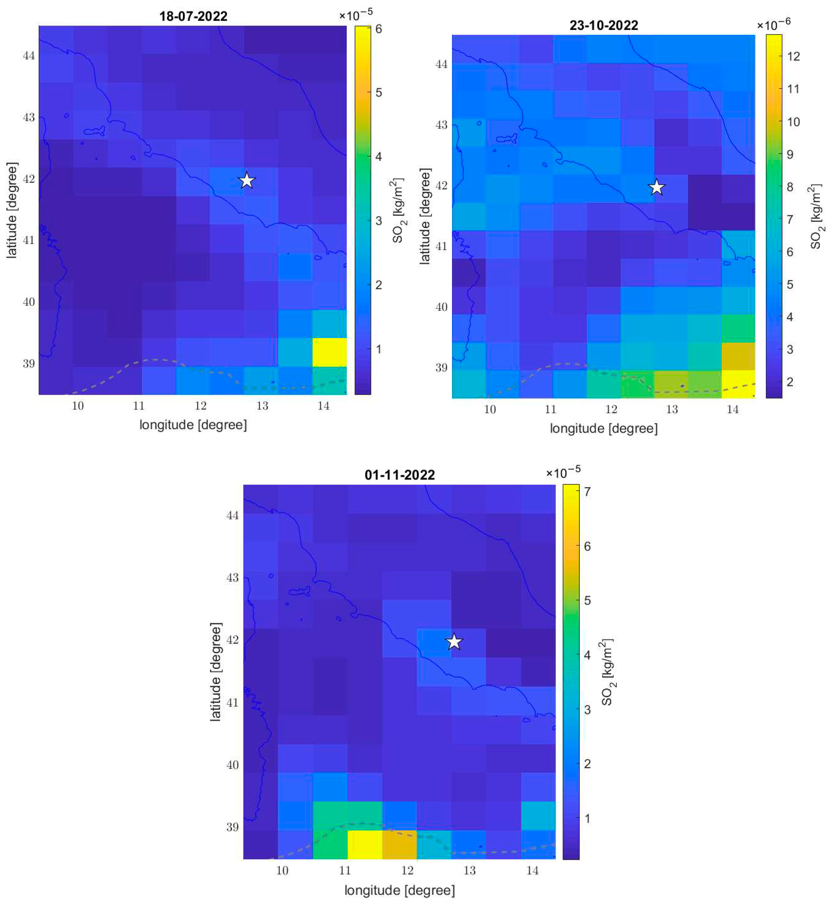
Figure 7.
Swarm Bravo magnetic field analysis on 6 August 2022, track 23. The title reports the first satellite letter, date of acquisition, track number, mean local time and UT time, geomagnetic indexes, and the total number of original samples acquired with anomalous ESA Swarm data quality flags. The map shows the projection of the satellite track in brown and eventual anomalous flags are marked with red. The green star represents the epicenter of M3.3 1 January 2023 Guidonia earthquake and yellow circle is the Dobrovolsky of an earthquake of magnitude 4.1. The residuals of geomagnetic signals for X-North, Y-East, Z-Center and absolute scalar intensity are represented with blue lines on the left with correspondence with the map and eventual anomalies inside the research area are marked with red lines.

Figure 8.
Swarm Bravo magnetic field analysis on 16 December 2022, track 22.
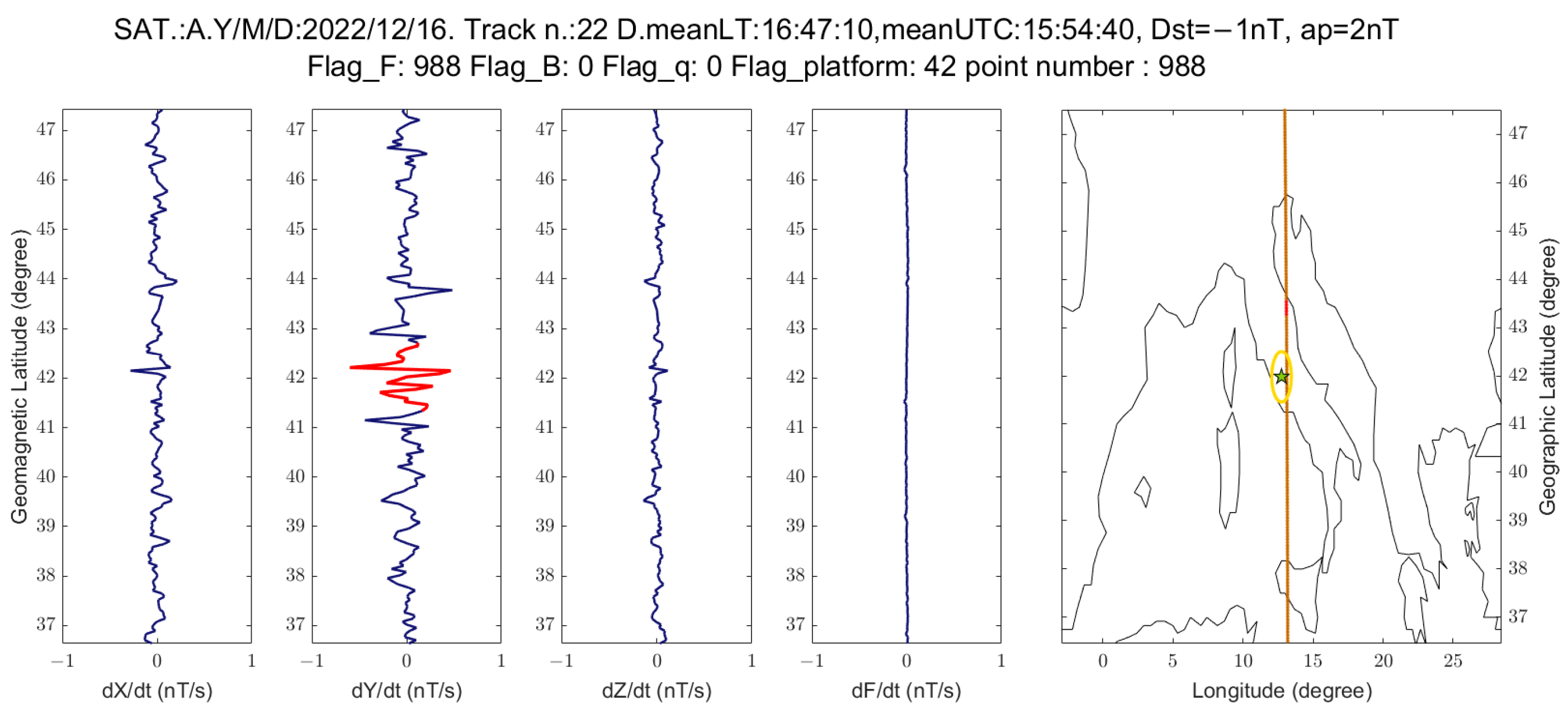

Table 1.
List of the tested magnitudes with the corresponding Dobrovolsky’s radius.
| Estimated magnitude | Doborovolsky radius [km] |
|---|---|
| 3.3 | 26.2 |
| 3.5 | 32.0 |
| 3.7 | 39.0 |
| 3.9 | 47.5 |
| 4.1 | 57.9 |
| 4.3 | 70.6 |
| 4.5 | 86.1 |
| 4.7 | 105.0 |
Table 2.
List of the Swarm anomalous tracks in the research area defined by the Dobrovolsky’s radius of M=4.1.
Table 2.
List of the Swarm anomalous tracks in the research area defined by the Dobrovolsky’s radius of M=4.1.
| Swarm | Date | Time UT | Local time | Anomalous component |
|---|---|---|---|---|
| Bravo | 17 July 2022 | 07:04:03 | 07:57:16 | X-North |
| Bravo | 6 August 2022 | 17:06:22 | 17:56:06 | Y-East |
| Bravo | 14 August 2022 | 04:44:07 | 05:33:49 | X-North |
| Alpha | 16 December 2022 | 15:54:40 | 16:47:10 | Y-East |
Disclaimer/Publisher’s Note: The statements, opinions and data contained in all publications are solely those of the individual author(s) and contributor(s) and not of MDPI and/or the editor(s). MDPI and/or the editor(s) disclaim responsibility for any injury to people or property resulting from any ideas, methods, instructions or products referred to in the content. |
© 2023 by the authors. Licensee MDPI, Basel, Switzerland. This article is an open access article distributed under the terms and conditions of the Creative Commons Attribution (CC BY) license (http://creativecommons.org/licenses/by/4.0/).
Copyright: This open access article is published under a Creative Commons CC BY 4.0 license, which permit the free download, distribution, and reuse, provided that the author and preprint are cited in any reuse.


