
Submitted:
22 May 2023
Posted:
23 May 2023
You are already at the latest version
Preprints on COVID-19 and SARS-CoV-2
Abstract
In this age of mass media and, in particular, social media-driven perception of reality, coupling disease and prophylactic opinion dynamics models can provide better insights into disease evolution than using a disease model alone. We develop in this work two disease-opinion dynamics models based on the epidemiology of the new coronavirus disease (COVID-19) and the availability or not of imperfect vaccines. We assume that susceptibility to infection decreases with the level of prophylactic attitude (personal hygiene, social distancing), and changes in prophylactic attitudes of susceptible individuals occur in response to perceived disease prevalence and vaccination coverage and efficacy in the population. We derive and discuss the disease-free equilibriums and reproduction numbers in the introduced models. We further assess the impacts of the distribution of opinions at disease introduction, the ability to detect presymptomatic, asymptomatic and symptomatic positive COVID-19 cases, the behavioural responses to the outbreak and the introduction of vaccination, and the effects of distortions of disease prevalence by public policy and mass media on disease dynamics. The insights highlighted from the proposed models are expected to make informative contributions to public policy in a context of opinion fluxes in response to perceived disease prevalence.
Keywords:
COVID-19
; Disease-behaviour dynamics model
; Prophylactic attitude
; Vaccination
; Perceived disease prevalence
1. Introduction
The emergence in late 2019 of the new coronavirus disease (COVID-19) caused by the pathogen SARS-CoV-2 is a devastating example of highly contagious emerging infectious diseases in response to increases in the magnitude and rate of overexploitation, habitat loss, global loss of biodiversity and climate change that many studies have warned against during the last decades [1,2,3,4]. The COVID-19 pandemic has impacted social and cultural habits, recreational and economic activities, laws and rights, among other aspects of the human civilisation. Increases in the levels of personal hygiene and social distancing from perceived sources of infection have shown significant potential to reduce the transmission of SARS-CoV-2 and thereby the spread of COVID-19. But the spread of a contagious disease in this era of mass media and connected populations is inevitably concomitant with the dissemination of antagonist information and opinions on the related pathogen, disease and prophylactic measures [5,6,7,8].
Modeling disease dynamics is the unique route to circumventing, containing, anticipating and preventing or reducing the ravages by deadly emerging or re-emerging infectious diseases. The numerous recent epidemic outbreaks (e.g. MERS, SARS, Ebola) have indeed urged the development of mathematical and statistical models for the spread dynamics of the particular diseases. Many such models include opinions regarding vaccination [9,10,11]. Indeed, vaccines’ safety and use have always and everywhere raised controversial issues [12,13,14]. For instance, controversies about COVID-19 vaccines have been widely spread once the first trials for safety and effectiveness assessment started, especially in highly connected social networks [15,16,17,18,19,20]. The opinions and the related attidudes toward vaccines have obvious consequences in the spread of diseases and their ability to cause epidemics [21]. Opinions on other prophylactic measures have however been less considered, although they can directly impact both transmission dynamics and attitudes toward vaccination. The dynamics of these other prophylactic behaviours can substantively differ from the dynamics of attitudes toward vaccination, because, for instance, they demand stronger engagement in terms of the required frequency of affirmation [22]. In the COVID-19 pandemic context in particular, hands need to be regularly washed when the environment is full of potentially contaminated areas, face masks need to be worn when using any shared public space, and minimum social distance needs to be kept in mind when interacting with fellows.
The recent development of models coupling disease, economic and opinion dynamics [23,24,25,26,27,28,29,30,31,32,33,34,35,36,37,38] provides headways towards effective joint modeling of health-related beliefs and attitudes, economic constraints, public health utility, disease dynamics, and their interactions. Most of the current models primarily rely on quite simplistic assumptions such as the SIS [24,27,39], SIR [22,23,40,41,42] and SEIV models [43] for disease dynamics. However, for highly contagious diseases such as COVID-19, the world’s reactions to outbreaks generally involved isolating some infectious individuals from the susceptible population, making the distinction of “quarantined” individuals from other infectious individuals crucial for sound modeling of this disease [44]. Moreover, the epidemiology of COVID-19 indicates even more complex disease dynamics involving presymptomatic, asymptomatic, and symptomatic infectious states [45,46,47,48,49,50,51,52]. In such situations, the use of too simplistic models can neglect crucial characteristics of target diseases, and confound some distinct disease-opinion interactions important for decision making. In addition, although vaccination is also a prophylactic measure, the attitude toward vaccination may be inconsistent with other prophylactic behaviours. For instance, an individual with a low level of prophylactic behaviour may get vaccinated in order to ignore social distancing. Likewise, an agent with initially high level of prophylactic behaviour may become overconfident after vaccination and relax personal hygiene and social distancing, lowering its level of prophylactic behaviour [53]. Once vaccination is introduced in an epidemic context, it indeed becomes crutial for a sound modeling to account for the potential interactions between opinions on both basic prophylactic measures and vaccination, including reverse effets.
To tackle this background, we build on the work of Tyson et al. [22], by introducing a disease-opinion dynamics model framework that modulates the effective contact rate in the target population based on the perceived disease prevalence generated by public health policymakers and mass media. Specifically, we propose (1) a disease-opinion dynamics model that accounts for basic prophylactic measures against emerging infectious diseases, the related beliefs and behaviours, and important disease states based on COVID-19 epidemiology, and (2) a joint model integrating attitudes toward vaccination and other prophylactic measures with disease dynamics. It is worth noticing that Arthur et al. [27] have recently proposed a discrete–time SIR model with an effective contact rate modulated by an utility function with delayed information, allowing an adaptive and optimal control of the population’s effective contact rate. In addition to the use herein of a more realistic model for COVID-19 dynamics, our proposal differs substantially from their model in regards to its construction joining two different mean field equations related to opinions and disease, and the direct insights it provides on the processes governing changes regarding opinions or disease, and their interactions. Moreover, unlike Arthur et al. [27], we do not assume that susceptible individuals rationally find an optimal contact rate by trading off how many people they want to interact with versus their risk of becoming infected. We rather consider a social influence approach [22] wherein a susceptible with a given opinion can change attitude in response to interaction with susceptibles holding a different opinion, the rate of such influences being determined by the perceived risk of becoming infected.
The objectives of this work are (i) to summarize the population dynamics (as expressed by the effective reproduction number for each introduced disease-opinion dynamics model) as a function of influence rate, rates of detection (testing policy) and isolation (“quarantining”), and vaccination rate, and (ii) to assess the impacts of the initial distribution of behaviours, nature of behavioural responses, rates of detection and isolation, initial vaccination coverage, efficacy of vaccines, vaccination rate, and distorted perception of disease prevalence on disease dynamics. The use of the proposed models is expected to make informative contributions to public policy in a context of opinion fluxes in response to perceived disease prevalence.
2. The Disease-Opinion dynamics models
We develop a generalization of the SIR–Opinion dynamics model [22] to suit the epidemiology of the pathogen SARS-CoV-2, the related coronavirus disease (COVID-19), and the availability of imperfect COVID-19 vaccines. On the one hand, we consider a disease evolution model distinguishing the infectious population into presymptomatic, asymptomatic and symptomatic individuals, and possibly the susceptible population into unvaccinated and vaccinated individuals. On the other hand, we extend the prophylactic opinion spectrum of Tyson et al. [22], introducing a prophylactic opinion field where attitudes/opinions toward both standard prophylactic measures (e.g. personal hygiene, face mask wearing and social distancing) and vaccination, and their interactions are integrated.
2.1. Disease dynamics
We describe disease evolution using a compartmental model in which the target population is basically structured into Susceptible (S), Exposed (E), Infectious (I), Quarantined (Q), and Recovered individuals (R) [54,55,56]. But the infectious population is further distinguished into presymptomatic (), asymptomatic (), and symptomatic infectious () individuals, whereas the susceptible population (S) is distinguished into unvaccinated and completely susceptible individuals (U), and vaccinated and partially immunized individuals (V). The sizes of the susceptible and the infectious compartments satisfy respectively and at time t, and the total population size is given by
In a vaccination-free context (e.g. for a new emerging disease), the size of the vaccinated population is zero () and the susceptible population consists of only unvaccinated individuals (). We have in this case a SEIQR model which is appropriate for the early phase of the COVID-19 pandemic. When vaccines become available, we have the more general UVEIQR model.
For simplicity, the susceptible population (S) is assumed homogeneous with regards to factors such as age and medical conditions. We account for natural human demography, i.e. we include a natural death rate () for the whole population, and assume a constant timely number of new births and net immigration () entering the class S of susceptibles (i.e. there is no immigration of infectives). Moreover, because isolated infectious individuals do not mix actively with other classes, we assume that they do not have adequate contacts (i.e. contacts sufficient for transmission) with susceptible individuals [57,58,59]. Under the corresponding “quarantine-adjusted incidence” mechanism [60], the force of infection defined as the expected number of adequate contacts of one susceptible person with infectives per unit time (i.e. the rate at which new infections (E) are produced), is given at time t for a completely susceptible individual by
where , and are baseline rates of effective contacts by presymptomatic, asymptomatic, and symptomatic infectious individuals, respectively. The available vaccines are considered imperfect, with an average efficacy of vaccine-induced protection . In other words, contacts between a V individual and , or individuals can be sufficient for transmission, but the force of infection is reduced to . A detailed description of both the SEIQR and the UVEIQR disease dynamics models in line with the known epidemiology of COVID-19 is given in Appendix A, along with graphical representations and mathematical descriptions based on nonlinear differential equations.
2.2. The Prophylactic attitude spectrum
In a vaccination–free epidemic context, we follow Tyson et al. [22], assuming for simplicity that opinion dynamics only occur within the susceptible population S. The latter is distinguished into three groups of individuals that can be identified based on the level of prophylactic behaviour which takes values in the prophylactic attitude spectrum:
For any opinion , denotes susceptibles with attitude i: represents individuals with the highest level of prophylactic behaviour (and thus the least susceptible to the disease), and corresponds to individuals with the lowest level of prophylactic behaviour (and thus the most susceptible to the disease). Individuals in the middle of the spectrum correspond to an intermediate level of prophylactic behaviour. Note that if the opinion is opposed to , then our model includes individuals with completely neutral position (), unlike in the binary voter model based spectrum used by Tyson et al. [22]. However, the spectum (3) simply defines the intensity of prophylactic behaviour on an ordinal scale, and high level attitude () is not necessarily opposed to low level attitude (). The identity holds for the susceptible population at time t.
2.3. The source and rate of opinion dynamics
Opinion dynamics results from changes of opinions and behaviours over time, for instance, as the mass media diffuse information about disease prevalence or evolution of the pathogen, or as disease surveillance and control policies are introduced or modified. We adapt here the “influence” approach of Tyson et al. [22], opinions being updated in response to interactions between susceptibles along the prophylactic opinion spectrum (3). In this framework, opinion dynamics within the susceptible population is governed by the rates (i.e. amplitudes) and the directions of mutual opinion influences.
The rate at which a susceptible individual influences the rest of the susceptible population is referred to as “influence function”. For their SIR-Opinion dynamics model, Tyson et al. [22] introduced linear and saturating influences as functions of the proportion of the infectious population (I). We consider here influence functions of the form
where are Tyson et al. [22]’s fixed-order saturating extreme influence weights, and is the “perceived disease prevalence”. The influence weights are given for by
with , the baseline influence rate for extreme opinions; , a skewness parameter; and , a half-saturation constant (see Appendix B for a graphical overview of ). In Equation (4a), we have substituted a perceived disease prevalence to the proportion of infectious (I) used by Tyson et al. [22], because, in our SEIQR model framework, the true disease prevalence given by is unknown to any individual in the population (only Q is observable), and estimates of P reported by the mass media are perceived as disease prevalence (see details on recovering P from epidemic and medical data in Appendix (Appendix C)). The perceived disease prevalence is a determinant of opinion dynamics [61,62], and indeed, a source of changes in the rates of influences on and by prophylactic opinions, as implied by Equation (4a). Clearly, the under or over estimation and reporting of disease prevalence by media or public health policymakers play a role in opinion dynamics.
In regards to the directions of influences, when an individual influences an individual the individual changes its attitude by moving one step towards i [22]. For instance, if the two individuals are at the opposite sides of the attitude spectrum (i.e. ), then the individual changes its attitude by moving one step towards the other side (i.e. ). If on the contrary the interacting individuals have the same opinion (i.e. ), no change occurs. When an individual at a given side of the attitude spectrum () influences a moderate opinion holder , then . Finally, when an individual at a side of the spectrum () is influenced by an individual, then . These changes of opinions in the susceptible population can be summarized by the rates of outgoing flows (opinion change ) as:
2.4. The SEIQR-Opinion dynamics model
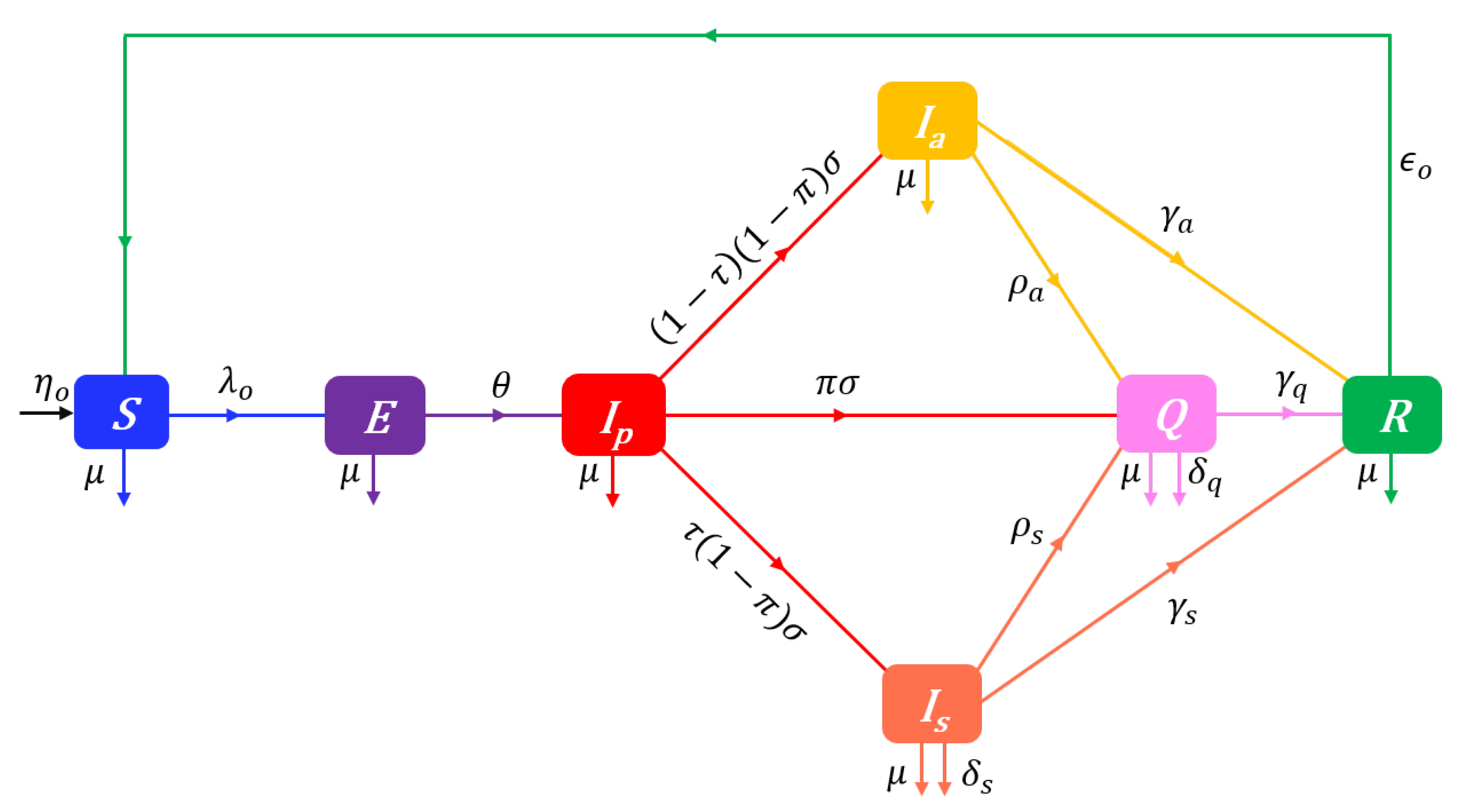
The proposed SEIQR-Opinion dynamics model is depicted on the flow diagram in Figure 1.
Note the use in Figure 1 of opinion-specific forces of infection (). Indeed, since increased levels of personal hygiene or social distancing from perceived sources of infection can substantively reduce both contacts and, if any, the sufficiency of contacts for transmission, we assume that an individual’s attitude determines its susceptibility to infection in a way such that the force of infection for individuals has the form
where, for and , is the rate of contacts sufficient for transmission from an infectious to a susceptible. For simplicity, the dependence of infection rate on attitude is modeled using a single parameter [22]. It is specifically assumed that, for each infectious class , the sufficient contact rate is given by , i.e.
where is the baseline rate of sufficient contacts with infectious (this applies to susceptible individuals who have the lowest level of prophylactic behaviour), and .
From the structuring of the susceptible population S in terms of prophylactic opinions i, the overall force of infection in the whole target population is given by the weighted average . The SEIQR-Opinion dynamics model is described at time t by the following system of nonlinear differential equations:
with the nonnegative initial conditions , , , , , , and where , and for . In System (Section 2.4), the dots represent partial derivatives with respect to time (t), denotes the time-dependent outgoing flows rate from susceptibles:
, , and the constant rate parameters of the model are described in Table 1. We shall use the qualifier “disease-dependent” for any solution for which there exists a finite time such that .
2.5. The prophylactic attitude field
In addition to preventing infectious diseases through immunisation, vaccines have further benefits such as reduced antimicrobial resistance and herd protection to unvaccinated individuals, including the elderly with waning immune systems and those who are too young to be vaccinated, or are immunosuppressed due to particular medical conditions [63,64]. Because vaccines come with potential safety and efficacy concerns, their obvious advantages do not prevent controversies which feed a vaccine related opinion dynamics, especially in highly connected social networks [15,16,17,18,19,20]. As a result, a disease–opinion dynamics model must account for the impact of vaccination on both attitudes and disease transmissions once vaccines are introduced into an epidemic context.
The fact that the attitute towards vaccination may be inconsistent with other prophylactic behaviours advises against the use of one scale between two extreme opinions on prophylactic measures in an epidemic context involving vaccination. Hence, we consider that the prophylactic opinion spectrum in Equation (3) excludes opinions on vaccination. A spectrum of vaccination-related opinion is separately introduced into the model, resulting in a bivariate field of opinions. For simplicity, we consider only two antagonists opinions toward vaccines: favourable and unfavorable [11]. The bivariate attitude field is defined as
where for each element , and , indexes individuals unfavourable to vaccination, and indexes individuals favourable to vaccination. In consequence, a class of susceptibles () is further structured into three groups: completely susceptible individuals unfavorable to vaccination (), completely susceptible individuals favorable to vaccination (), and susceptibles with active vaccine-induced immunity (). The total susceptible population is then given by where denotes all completely susceptible individuals, denotes completely susceptible individuals unfavorable to vaccination, denotes completely susceptible individuals favorable to vaccination, and denotes vaccinated individuals. The identity still holds for the whole susceptible population, and in addition, where .
2.6. Changes in prophylactic attitudes in the presence of vaccination
We still assume that opinion dynamics only occur within the susceptible population (S), including , and V individuals. Changes of opinion on prophylactic behaviours (excluding vaccination) are determined within , or V individuals by an “influence” process. Assuming for simplicity that the influence rates are ceteris paribus the same within the pro-vaccine and anti-vaccine susceptible populations as well as in the vaccinated population, the rates of outgoing flows (opinion change ) are defined by analogy to Equations (5a)–(5d) as:
where are influence functions. As the vaccination-free influence function defined in Equation (4a), the influence function depends on the perceived disease prevalence . However, in a vaccination-dependent epidemic context, vaccine coverage (i.e. the proportion of vaccinated individuals), which is widely publicised in the mass media, is also expected to impact prophylactic behaviours. It appears that when the influence of an individual with an opinion i increases with , then it will likely decrease with vaccine coverage (see e.g. [53]) and vice-versa. Assuming independence between the relative importances of and V in , the influence rate is given the form
so that if , i.e. Equation (10e) is reduced to Equation (4a) in a vaccination-free context, and irrespective of vaccine coverage, remains the initial influence rate of an extreme opinion holder when the disease is not perceived (, i.e. an actual disease-free context, or a failure to detect any infectious individual although ). It is worth noting that the basic influence is a decreasing function for and an increasing function for (see graphics in Appendix B, see also Figure 1 in [22]). As a result, the influence of a high level prophylactic attitude () increases with the perceived disease prevalence but decreases with vaccine coverage. Conversely, the influence of a low level prophylactic attitude () decreases with but increases with . It also stems from Equation (10e) that vaccination () reduces the slope of the influence rate for all prophylactic opinions. Specifically, when of the population is immunized through vaccination, the influences of prophylactic opinions become less responsive to changes in the perceived disease prevalence , as compared to the response in a vaccination-free context.
2.7. Changes in attitudes towards vaccination
We consider that changes of opinion on vaccination within individuals ( and ) are also governed by an “influence” process. Assuming that changes of attitude toward vaccines is independant of the level i of prophylactic behaviour, the rate at which individuals lose conviction to vaccination benefits and return to the class , and the rate at which individuals become favourable to vaccines and enter the class are given for any opinion by
where and are influence functions related to opinions on vaccination. Note that individuals with vaccine-induced immunity (V) are all assumed to be favourable to vaccines (at least until the temporary immunity vanishes). To obtain simple expressions for the influence functions and , we assume that there is no change in vaccine related opinions when the disease is not perceived (), and the influence rates of pro-vaccine and anti-vaccine susceptibles are also constants when , i.e. there is no shift in vaccine related opinions until vaccination begins (note that this assumption is not as restrictive as it may first appear, because we have once trials for vaccine safety and efficacy start in the population, or even when only , i.e. vaccinated individuals only flow in from abroad). We also assume that an increase of either or leads to an increase in the influence of pro-vaccine susceptibles, but to a decrease in the influence of anti-vaccine susceptibles. From these assumptions, we define the influence functions as:
It appears from these expressions that when the perceived disease prevalence increases by , the influence of any vaccination related opinion becomes more responsive to changes in the vaccine coverage .
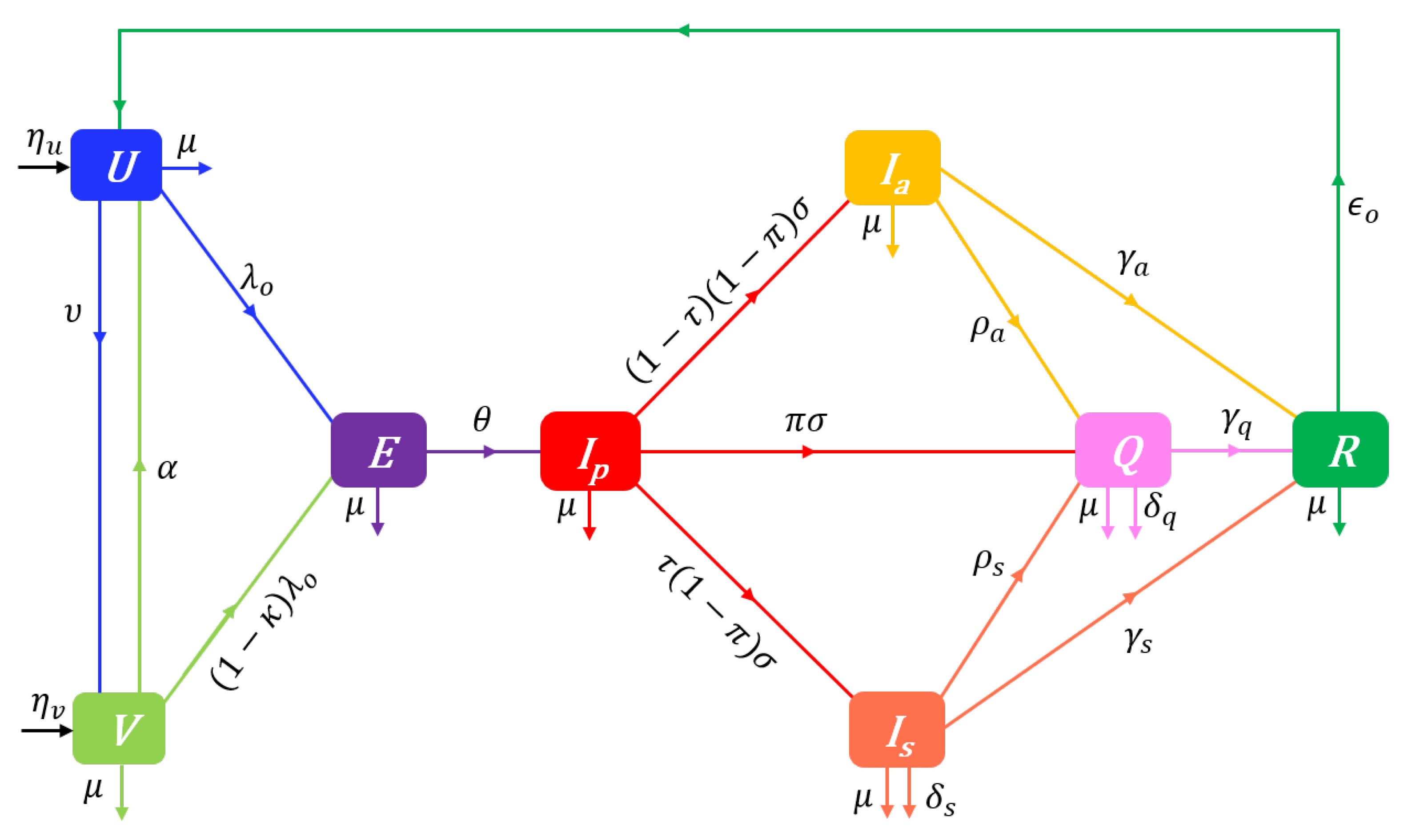
2.8. The UVEIQR-Opinion dynamics model
We build a Disease-Opinion dynamics model by integrating prophylactic behaviours and vaccine related opinions into the UVEIQR model. With the vaccination process, pro-vaccine susceptibles who have the prophylactic opinion i () get vaccinated (and enter the class ) at the same rate (irrespective of i). Likewise, the vaccinated individuals in lose their immunity and return to the class at the rate . We also assume that anti-vaccine susceptibles () do not get vaccinated.
The opinion-specific force of infection is given by Equation (6a) for individuals, and is for individuals. The overall force of infection in the whole population is then given by the weighted average
The flow diagram of the UVEIQR-Opinion dynamics model is shown in Figure 2.
Let denote for the opinion-related incoming flows for susceptible states:
and let denote the time-dependent outgoing flow rates:
The proposed model is described at time t by the following system of differential equations:
with the nonnegative initial conditions , , , , , , , and where and for and , and . In Equations (14a)–(14o), , (e.g. for an equal repartition; or and assuming that 50% of recovered individuals have a moderate prophylactic attitude), and the constant rate parameters of the model are described in Table 1.
Note that in the special case and for , model (14) is reduced to the vaccination-free model (7) where susceptibles are divided into and with constant mutual influence rates (but with no incidence on disease dynamics or basic prophylactic opinion dynamics).
3. Analytical results
The first important property of any mathematical model for a biological process is, of course, biological meaningfulness. The following result guarantees that the UVEIQR-Opinion model always has a biological interpretation.
Lemma 1
(Non-negativity and Boundedness). Under the nonnegative initial conditions , , for , , , , , and , all solutions of Systems (14) remain nonnegative and are bounded at any time . The total population size is in particular bounded as where with the carrying capacity in disease–free conditions.
Since System (7) is a special case of System (14), Lemma 1 also assures that all solutions of the SEIQR-Opinion model (7) are biologically meaningful. In the remainder of this section, we present some important properties of disease-opinion dynamics in a population described by the introduced models. The analogous mathematical properties for the models with no differential opinion are given in Appendix A.3, and the proofs of all results are given in Appendix D. Unlike in Lemma 1, we start for clarity with the properties of the simpler model (7) without vaccination ( and for ) and then discuss the changes induced by the introduction of vaccines in both disease and opinion dynamics in the model (14).
3.1. Vaccination–free disease–free equilibrium and reproduction numbers
To summarize the dynamics of a population described by the SEIQR-Opinion model (7), we find the disease-free equilibrium (d.f.e.) of the model and use it to obtain the effective reproduction number by the next-generation matrix approach [65]. We further derive critical detection rates to potentially achieve disease eradication in the long run.
Proposition 1
(Vaccination–free d.f.e. & Reproduction number). The SEIQR-Opinion model (7) has a unique d.f.e. given for by
When , we have for . Moreover, for a population described by System (7), the basic reproduction number is given by
is the contribution of susceptibles and infectious to , with , , and . Furthermore, the basic reproduction number decreases with the baseline influence rate (provided that the prophylaxy-induced infection rate reduction factor satisfies ). The time-varying effective reproduction number is given by
Remark 1.
In the absence of opinion dynamics (), each class of susceptibles approaches its carrying capacity .
Remark 2.
The stationary sizes of and susceptibles decrease with the baseline influence rate whereas increases with . Indeed, the mutual influences of and individuals () balance and cancel each other whereas interactions between individuals on the opposite sides of the attitude spectrum all lead to positive flows into . As a result, if for instance the recruitment rates are equal across susceptible states (), then more than the third of the long run population will have a moderate level of prophylactic attitute in the absence of disease. The decay of the basic reproduction number as a function of the baseline influence rate is another consequence of this stationary dynamics.
Remark 3.
If the prophylaxy-induced infection rate reduction factor equals one (no substantive differential prophylactic attitude despite opinion changes), we would expect disease dynamics to be independent of opinion dynamics. Accordingly, if .
Remark 4.
The basic reproduction number accounts for the implementation of a disease surveillance mechanism if any (i.e. the detection rates π, and can be positive even in a disease-free context). In an emerging disease context (e.g. right before the report in late December 2020 of the first confirmed COVID-19 case), some symptoms might be unknown, test kits might not be yet developed or available. In the special case where , the basic reproduction number is
which satisfies ceteris paribus.
The first measures implemented after the epidemic outbreak of a contagious disease is the identification and isolation of infectious individuals. The detection/isolation effort (targeting and testing of most susceptible groups, contact tracing, voluntary mass testing campaign, systematic testing) is critical to the control of the propagation of the disease in the absence of vaccination. Such measures can be sufficient to contain an epidemic under some conditions detailled in the following corollary of Proposition 1.
Corollary 1
(Critical Detection Rates). Suppose that .
If , then the critical (minimal) early detection probability required to sufficiently lower and ensure disease eradication in the long run is
which decreases with the baseline influence rate , and the detection rates of asymptomatic infectious and of symptomatic infectious. If , then the critical (minimal) detection rate of asymptomatic infectious is
which decreases with π, , and . Likewise, if , then the critical (minimal) detection rate of asymptomatic infectious is
which decreases with π, , and .
It appears that if under an hypothetical (and unrealistic) scenario where all infectious individuals are isolated at the presymptomatic stage, then mass testing and quanrantining can be sufficient to ensure that an epidemic is unsustainable in the target population. If , then it is not possible to contain the epidemic of the target contagious disease using isolation measures only. It remains however possible to break the transmission dynamics by reducing exposition to the disease, i.e. the rate of sufficient contacts between potentially infectious and susceptible individuals (for COVID-19, this included e.g. social distancing, face mask wearing, school closing, curfew, ban of gatherings, lockdown). The introduction of vaccination is the ultimate solution to reduce transmissions while alleviating the social and economic drawbacks of the first containment measures.
3.2. Disease–free equilibrium and reproduction numbers in a vaccination context
We find the d.f.e. for a population described by the UVEIQR-Opinion model (14), and compute the related control reproduction number. We further discuss the critical vaccination rate to ensure disease eradication in the long run.
Proposition 2
(Disease–free Equilibrium & Reproduction Number). The UVEIQR-Opinion model (14) admits a unique d.f.e. given for by
where is given by
where we have set , and , , , , and denotes the identity matrix. In the absence of opinion dynamics (), we have , , and for .
Moreover, for a population described by System (Section 2.8), the control reproduction number is given by
is the contribution of susceptibles and infectious to , with . The control reproduction number decreases with the vaccination rate υ and the baseline influence rate , and satisfies
The time-varying effective reproduction number is given by
Remark 5.
The expression of in matrix notation given by Equation (19b) is developed in Appendix E where a formula is provided for each of the nine elements of .
It appears from Equation (20a) that, as expected, decreases with both vaccination rate () and average vaccine efficacy (), but increases with the immunity lost rate (). Inequality (20b) recognizes that vaccine efficacy is an important parameter in disease control: cannot fall under even for a large vaccination rate . On setting
for , a necessary condition for disease eradication is that the average vaccine efficacy must satisfy (ensuring ). The following corollary gives the critical vaccination rate to eradicate the disease for a fixed average vaccine efficacy .
Corollary 2
(Critical Vaccination Rate). If and , then the critical (minimal) vaccination rate required to sufficiently lower and ensure disease eradication in the long run is
which increases with the immunity lost rate α, decreases with κ, and satisfies
3.3. Stability of disease–free equilibriums and persistence of the disease
The following results establish the stability of the disease-free equilibrium (15a).
Lemma 2
(Local Asymptotic Stability of the Disease–free Equilibrium). The disease-free equilibrium of the SEIQR-Opinion model (7) is locally asymptotically stable if , and unstable if .
Proposition 3
(Global Asymptotic Stability of the Disease–free Equilibrium). The disease-free equilibrium of the SEIQR model (7) is globally asymptotically stable, i.e. for any solution , , provided that .
If , then the d.e.f. (19a) is not stable, and any introduction of infectious individuals has the potential to kick off and maintain an epidemic outbreak, as per the next proposition.
Proposition 4
(Disease Persistence). Let us consider the UVEIQR-Opinion model (14). If , then the disease persists uniformly, i.e. there exists a positive real constant ϱ independent of the initial data, such that for any disease-dependent solution , we have:
4. Numerical results
4.1. Impacts of the initial distribution of behaviours
Responses: , , ,
Responses: (true) peak time , observable peak time ,
Responses: (true) epidemic peak size , observable epidemic peak size ,
Responses: epidemic duration , final (true) epidemic size, observed epidemic size
Responses: basic, control and effective reproduction numbers
4.1.1. Vaccination-free dynamics
Vary presence/absence of opinions; influence functions/parameters
Vary the initial proportion of different prophylactic opinions
4.1.2. Vaccination-dependent dynamics
Vary the initial vaccine coverage (proportion of vaccinated individuals)
Vary the initial proportion of pro-vaccine susceptibles
Vary the initial proportion of different prophylactic opinions (by vaccine-opinion)
Vary vaccination rate
4.2. Impacts of the nature of behavioural responses
The above responses
Vary influence parameters (relative to ), and
(Also vary the initial proportion of different prophylactic opinions)
4.3. Impacts of detection rates and distorted perceived disease prevalence
The above responses
Vary early detection probability and late detection rates and .
Vary the estimates of mean residential times , ,
and around their true values so that the perceived disease prevalence under/over estimates the true disease prevalence.
5. Discussion and conclusion
5.1. The impact of opinions on disease dynamics
5.2. The behavioural response to vaccination
5.3. The impact of distorted perceived disease prevalence
5.4. Limits and perspectives
Because of the relatively large number of possible states given the considered disease and opinion dynamics, some simple assumptions were made in the model construction in order to reduce the number of model parameters on the one hand, and mostly to obtain a minimum of analytical closed form results on the other hand. Ahead is the use of a unique class of exposed individuals, irrespective of the vaccination status of the individuals before exposition. Although this assumption may hold for some diseases, it is not realistic in the ongoing COVID-19 pandemic context, because the effects of the currently available vaccines are beyond a mere reduction in the force of infection. Indeed, the vaccines also reduce the risk of severe forms of the disease (requiring respiratory assistance), transmission from vaccinated infected, risk of long term sequels, and disease-related mortality [66,67], so that the paths from exposition to recovery should be different for vaccinated individuals as compared to non vaccinated individuals. In addition, no age structure is included in the proposed models, although COVID-19 transmission and mortality rates, as well as vaccination scenarios are highly age dependent [68,69,70,71]. Another source of complexity we did not account for is the co-existence of many variants of SARS-CoV-2 with different transmission and mortality rates in a target human population [72,73].
Many strong assumptions were also made in regards to opinion dynamics. The strongest one is likely that opinion dynamics only occur in the susceptible population. As in Tyson et al. [22], this assumption simplifies model equations a lot. Though, all individuals in disease-dependent states, including the non-mixing population Q (which can interract with susceptibles by e.g. cell phone, social media, ...), can obviously influence the opinions of susceptibles. For instance, the prophylactic opinions of physically isolated (Q) and recovered (R) individuals can change in response to being aware of their current or past infectious states. These opinion dynamics can then contribute to the overall influence of a given opinion i holders on susceptibles who have a different opinion . Clearly, as for susceptibles, disease-dependent classes should also be differentiated according to opinions, and their interactions with other classes allowed to influence, to some extent, the attitude of susceptible individuals. Another strong assumption is the consideration of only one prophylactic attitude level for each prophylactic opinion. This hypothesis supposes that all individuals with a given opinion have the same prophylactic attitude level (same degree of opinion), and thereby hides interactions between like-minded individuals. In consequence, the assumption neglects amplification of opinion, a phenomenon which can substantially impact opinion dynamics [22].
In reality, the actual attitude of a susceptible individual depends not only on its opinion, but also on the enforcement of any restriction by local and national governements. The restrictions, often referred to as non-pharmaceutical interventions (NPIs) can significanly affect effective contact rates depending on the stringency of the measures. A more realistic model should indeed account for the NPIs enforced by governements in the baseline contact rate by each infectious class j. Since NPIs are functions of time, so should be the contact rates. A more general model could thus consider contact rates of the form with , where is the baseline contact rate when no NPI is implemented, is a vector of uncorrelated indexes measuring the intensity of NPIs, and is a vector of regression parameters linking to .
An additional key assumption is that all individuals have the same baseline influence rate in disease–free conditions, irrespective of prophylactic opinion. Instead of Equation (4b), the basic influence weights could have, for , the more general form
where is a baseline influence rate reduction factor for a moderate opinion. In Equation (24a), the parameter allows to reduce the influence rate of moderate prophylactic opinion holders () relative to extreme opinion holders (). The model presented in Section 2 corresponds to the special case . In this modified influence process based on Equations (4a) and (24a), Equation (10e) defining influence rates in a vaccination-dependent context becomes
The resulting extended SEIQR-Opinion model admits, for and , disease-free equilibriums of the form where
where , returns the positive roots of the quartic polynomial defined for x as , with the kth element of the vector , , , , , and . For , Remark 2 does not hold in general. Indeed, it turns out that the extended model can admit up to three DFEs, so that, as in the SIR-Opinion model of Tyson et al. [22], the basic reproduction number depends on the initial distribution of the population along the attitude spectrum. Nevertheless, in the special case (i.e. when the recruitment rates of individuals holding the two extreme opinions have the same shares in the total recruitment rate ) with opinion dynamics (), the extended SEIQR-Opinion model has a unique d.f.e. where we have and Equation (25b) is simplified to
with . Here, the number of moderate opinion holders at the d.f.e. increases not only with the baseline influence rate (as in Remark 2), but also with the influence rate reduction factor , so that the basic reproduction number decreases with both and . The study of the extended model could thus uncover interesting changes in opinion and disease dynamics.
Funding
This research received no external funding.
Institutional Review Board Statement
Not applicable.
Data Availability Statement
The authors confirm that the data supporting the findings of this work are available within the article.
Conflicts of Interest
The authors declare no conflict of interest.
Appendix A. The disease dynamics models
Appendix A.1. The extended SEIQR model
The models considered for disease dynamics distinguish two different states during the pathogen incubation period when exposed individuals do not develop any COVID-19 symptom: the simple Exposed (E) state for non-infectious individuals, and the presymptomatic state () for infectious individuals. The simple exposition period lasts (up to 14 days [48], but generally short, i.e. about six days) and is followed by the presymptomatic period (which lasts ) during which incubating individuals become infectious but remain without symptom [47,48,49,50,51,52]. Contacts between susceptibles and presymptomatic infectious () can be sufficient for transmission (see e.g. [45] and [46]). When control measures such as contact tracing and systematic tests on target groups are implemented, some presymptomatic infectious are detected with probability and “quarantined” (i.e. isolated) at home, hospitals or dedicated places. The remaining (undetected) presymptomatic infectious individuals evolve into two groups based on the development or not of COVID-19 symptoms: symptomatic infectious () and asymptomatic infectious (). Some of the symptomatic infectious individuals self-isolate or are detected and enter the class Q of quarantined at the rate . Again, contact tracing and systematic tests on target groups can lead to the detection and isolation of some asymptomatic infectious individuals at the rate . Symptomatic infectious () and isolated individuals (Q) die of COVID-19 at the rates and respectively. The alive asymptomatic infectious, symptomatic infectious, and quarantined individuals finally recover from COVID-19, at the rates , and respectively, and form the class of recovered individuals (R) who acquire a temporary immunity to SARS-CoV-2. Recovered individuals lose their immunity at the rate and become again susceptible to the pathogen. The flow diagram of the SEIQR model is depicted in Figure A1. The total population size at time is given by
Figure A1.
Flow-chart of a SEIQR model showing the flow of humans between different compartments. The susceptible population is denoted by S, and E, , , , Q and R denote respectively the exposed, the presymptomatic infectious, the asymptomatic infectious, the symptomatic infectious, the quarantined infectious, and the recovered populations. The parameters of the model are described in Table 1.
The SEIQR model is described at time t by the following system of differential equations:
with the nonnegative initial conditions , , , , , , and where . In System (A2), is the force of infection, and the constant rate parameters of the model are described in Table 1.
Appendix A.2. The UVEIQR model
Since many COVID-19 vaccines are currently distributed at various rates across the world, we allow the disease dynamics model to account for vaccine-induced immunity. For simplicity, we do not distinguish age groups although COVID-19 vaccination is widely implemented with different strategies and at different rates for childreen and adults [74,75,76]. Vaccines are primarily designed to prevent infectious diseases through the immunisation of vaccinated individuals [77,78], and thus increase the heterogeneity of the susceptible population S. Specifically, susceptible individuals are distinguished into an unvaccinated (and completely susceptible) population (U) which gets vaccinated at the rate , and a vaccinated (with active vaccine-induced partial immunity) susceptible population (V) which loses vaccine-induced immunity at the rate (the so called resusceptibility probability [79,80]). The timely number of net immigration (and new births) which enters the class of susceptibles is accordingly distinguished into unvaccinated () and vaccinated individuals () such that . The flow diagram of the UVEIQR model is shown in Figure A2 and the disease dynamics is described by the following system of differential equations:
 with the nonnegative initial conditions , , , , , and where and for any . In System (A3), is the force of infection in the completely susceptible population as given by Equation (2), , and the constant rate parameters are as described in Table 1. The total population size is given at time t by
Note that the UVEIQR model (A3) includes the SEIQR model (A2) as a special case when so that and for any . Also note that for the general UVEIQR model, the force of infection is reduced by a factor in the vaccinated population.
with the nonnegative initial conditions , , , , , and where and for any . In System (A3), is the force of infection in the completely susceptible population as given by Equation (2), , and the constant rate parameters are as described in Table 1. The total population size is given at time t by
Note that the UVEIQR model (A3) includes the SEIQR model (A2) as a special case when so that and for any . Also note that for the general UVEIQR model, the force of infection is reduced by a factor in the vaccinated population.
Figure A2.
Flow-chart of a UVEIQR model showing the flow of humans between different compartments. U is the unvaccinated (completely susceptible) population, V is the healthy vaccinated but partially susceptible population, E, , , , Q and R denote respectively the exposed, the presymptomatic infectious, the asymptomatic infectious, the symptomatic infectious, the quarantined, and the recovered populations. The parameters of the model are described in Table 1.
Appendix A.3. Mathematical properties
Since the SEIQR model (Appendix A.1) is nested into the UVEIQR model (Appendix A.2), we restrict attention to the latter, and then discuss the results in the special case . The proofs of the results are given in Appendix D.1.
- Non-negativity and boundedness
Lemma A1
(Non-negativity and Boundedness). Under the nonnegative initial conditions , , , , , , and , all solutions of System (A3) remain nonnegative and are bounded for all .
- Disease-Free Equilibrium and Reproduction Number
Proposition A1
(Disease-Free Equilibrium & Reproduction Number).
Set . The UVEIQR model (A3) admits the unique disease-free equilibrium
with the total population size at the carrying capacity .
Moreover, for a population described by System (A3), the basic reproduction number in a vaccination-free context (i.e. ) is given by
and once vaccination is introduced, the control reproduction number is given by
and satisfies
The time-varying effective reproduction number is given by
It appears from Equation (A5b) that, as expected, decreases with both vaccination rate () and average vaccine efficacy (), but increases with the immunity lost rate (). The inequality (A5c) recognizes that vaccine efficacy is an important parameter in disease control: cannot fall under even for a large vaccination rate . On setting
for , a necessary condition for disease eradication is that the average vaccine efficacy must satisfy (ensuring ). The following corollary gives the critical vaccination rate to eradicate the disease for a fixed average vaccine efficacy .
Corollary A1
(Critical Vaccination Rate). If and , then the critical (minimal) vaccination rate required to sufficiently lower and ensure disease eradication in the long run is
which increases with the immunity lost rate α, decreases with κ, and satisfies
Note that also decreases with , so that a positive net immigration of vaccinated individuals lowers the minimal required vaccination rate. The following lemma establishes local asymptotic stability conditions for the disease-free equilibrium point, and is further used to find global asymptotic stability conditions for the disease-free steady-state.
Lemma A2
(Local Asymptotic Stability of the Disease-Free Equilibrium). The disease-free equilibrium of the UVEIQR model (A3) is locally asymptotically stable if , and unstable if .
Proposition A2
(Global Asymptotic Stability of the Disease-Free Equilibrium). The disease-free equilibrium of the UVEIQR model (A3) is globally asymptotically stable, i.e. for any solution , provided that .
By Proposition A2, ensuring by for instance reducing contacts, susceptibility and transmissibility, or vaccinating a large part of the population, garrantees that the disease will die out shortly. If however , then any introduction of infectious individuals has the potential to kick off and maintain an epidemic outbreak, as per the next lemma.
•Persistence of the Disease and Endemic Equilibrium
Lemma A3
(Persistence of the Disease). Let us consider the UVEIQR model (A3) Let . If , then the disease persists uniformly, i.e. there exists a positive real constant independent of the initial data, such that any disease-dependent solution satisfies:
From Equation (A8a), it appears that in both vaccination-free (i.e. ) and vaccination-dependent contexts, the susceptible population size satisfies for any (since ). This is ensured by the positive rates of net recruitement (), recovery (), and immunity lost (). The persistence the of disease when implies positive disease endemism whose equilibrium is next characterized.
Proposition A3
(Endemic Equilibrium). If , then the UVEIQR model (A3) has no endemic equilibrium. When , the model admits the unique endemic equilibrium
where we have set , , , , , , , and ; the endemic force of infection is given by
with , and ; and the total population size is
The following results establish stability for the endemic equilibrium .
Lemma A4
(Local Asymptotic Stability of the Endemic Equilibrium). When it exists (), the endemic equilibrium of the UVEIQR model (A3) is locally asymptotically stable.
Proposition A4
(Global Asymptotic Stability of the Endemic Equilibrium). When it exists, the endemic equilibrium of the UVEIQR model (A3) is globally asymptotically stable, i.e. for any disease-dependent solution .
Note from Proposition A4 and Equation (A9k) that the persistence of disease () and the positive disease related death rates () reduce the long run population size below the carrying capacity .
Appendix B. Overview of fixed-order saturating influence functions
Appendix B.1. Vaccination–free influence functions
Plot the 3 influences for .
Appendix B.2. Influence functions accounting for vaccination
Build 3D plots of influences in terms of and V to support the claims.
Appendix C. Perceived disease prevalence
During epidemic outbreak times, many pieces of information related to the incidence of the disease are oftentimes publicised in mass media, social media, or in the streets. We indicate here how a consistent estimate of disease prevalence can be computed based on medical data, and highlight some alternative quantities that may be perceived as disease prevalence or risk.
Appendix C.1. Inferring Disease Prevalence from Medical Data
A variety of approaches have been used to estimate disease prevalence (see e.g. [81,82,83,84,85]). In this work, we assume that the perceived disease prevalence is equal to a consistent estimate of the true disease prevalence P, based on some consistent estimates of , , and . From our disease dynamics models (see Appendix A), the total number of timely new confirmed (positive) cases is
where is the mean residential time of infectious individuals in the class , is the early detection probability (during the presymptomatic incubation period), and and are late detection rates from the asymptomatic and symptomatic classes, respectively. We assume that the additive elements of are available based on medical surveys of newly identified cases, i.e. we have the presymptomatic new confirmed cases , the asymptomatic new confirmed cases , and the symptomatic new confirmed cases , such that . Likewise, we assume that medical surveys and observational data are available to compute some consistent estimates of the mean residential time of identified presymptomatic infectious in the class of presymptomatic infectives (i.e. ), of the mean residential time of identified asymptomatic infectious in the class of asymptomatic infectives (i.e. ), and of the mean residential time of identified symptomatic infectious in the class of symptomatic infectives (i.e. ). Then, , , and can be consistently estimated as
and is given for by
where has been substituted for to avoid doubly accounting for (since observations are always discrete although the UVEIQR model (Appendix A.2) is continuous).
Appendix C.2. Common measures of perceived disease prevalence
The daily number of positive new cases is a common measure of disease perceived disease risk . Other common measures include but , , [85],
Appendix D. Proofs of lemmas and propositions
Appendix D.1. Proofs of lemmas and propositions related to disease dynamics Only
Proof of Lemma A1.
From Equation (A3a), we have where (note from Equation (2) that is a majorant of ). This leads to:
The same argument gives , , , , , and and proves nonnegativity. Next, let . Then, by the nonnegative initial conditions and , we have . From Equation (1) and the System (Appendix A.2), we have
The last equation implies that . Integrating the later yields
with . It appears that as t increases, the upper bound of increases (when ) or decreases (when ) to eventually approach the carrying capacity as . Thus . Hence we overall have
The nonnegativity of , , , , , , and then implies that these quantities are all bounded, since their sum is bounded. □
Proof of Proposition A1.
Adding the disease-free restriction to System (A3) implies that . Setting all the derivatives to zero then gives and we are left with the system
which is solved for and through substitution, and the disease-free equilibrium (d.f.e.) in Equation (A4a) is obtained using . Next, let the vector of the compartments involved in the production of new infections or receiving new infections: . The corresponding subset of System (A3) has the form where
on setting . Then, letting , , , , , and , the Jacobian matrices of and evaluated at the d.f.e. are respectively given by
Following [65], the basic reproduction number is defined as the spectral radius (largest eigenvalue) of the next-generation matrix , and we find
Under the restriction , we have and . We thus have in this case (since ), and Equation (A5a) follows. Using the Equations (A4b) gives and Equation (A5b) follows. The expression (A5c) results from noting that decreases with and evaluating the limit to get an upper bound, and noting that also decreases with since , and evaluating the limit to obtain a lower bound. Finally, evaluating the Jacobian matrices of and at general values of U, V, Q, and N instead of the d.f.e. (i.e. replacing by ), results in Equation (A5d). □
Proof of Corollary A1.
We obtain by setting the expression (A5b) of to one, and solving for . It is obvious that increases with . From Equation (A7a), we get
hence decreases with , and is lower bounded by . □
Proof of Lemma A2.
lma:DFEquiStab0proof:lmaDFEquiStab0 A necessary and sufficient condition for an equilibrium to have local asymptotic stability (l.a.s.) is that all eigenvalues of the Jacobian matrix have negative real parts [86]. The Jacobian matrix of model (A3) at the d.f.e. has the block structure
, , , , and . From this structure, the eigenvalues of are those of , and (using Schur complements). We get the eigenvalues and from , and and from . Since for , we can next restrict attention to whose four eigenvalues must have negative real parts to ensure l.a.s.:
The characteristic polynomial of is
where , , and . The Routh-Hurwitz stability conditions (see Equation (A.22) in May [87]) corresponding to this polynomial are:
where . Since for any , we have (i): by definition (for any value of ). If , then . It follows that at least one eigenvalue of has a positive real part when , and unstability is established. When on the contrary, we have (ii): . Next, notice that is equivalent to . This implies that since and . Writing as
then shows that (iii): if . The statements (i), (ii) and (iii) ensure that all the four eigenvalues of have negative real parts when and l.a.s. is established. □
Proof of Proposition A2.
The proof uses a global stability result derived by Castillo-Chavez et al. [88]. Let and be the vectors of uninfected and infected classes, respectively, and set and . To establish global asymptotic stability (g.a.s.), we first show that the following conditions hold for the UVEIQR model (A3):
where is a Metzeler matrix (all off diagonal elements are nonnegative). To check , we set in System (A3) and get the reduced system
It comes that , and . Replacing the expression in and integrating the result leads to
It appears that and , both when (since ) and when . Then, leads to , hence holds. Next, using System (A3) and , and setting , we get
The matrix is obviously Metzeler. Moreover, the whole population is in the susceptible class S at the d.f.e., hence the maximal value of the average effective susceptibility in the mixing population , is . We thus have and so that holds. Then, by the Theorem in [88], the validity of the two conditions ( and ) ensures that the d.f.e. is g.a.s. provided that is l.a.s., i.e. (by Lemma A2). □
Proof of Lemma A3.
The proof is an adaptation of the proof of Theorem 3.3 in [89], originally built for dissipative dynamical systems. The primary aim is to find a positive sub-solution of the UVEIQR model (A3). Let and set . Note that the subset of System (A3) corresponding to (i.e. Equations (A3c)–(A3f)) can be compactly expressed as . We first show the existence of a pair of positive principal eigenvalue and eigenvector of this subset when . Linearizing the target subset of the system around the d.f.e. gives , where , i.e.
Substituting a solution of the form with , we get . Note that is a Metzeler matrix (i.e. for ). Therefore, is irreducible if and only if the matrix (with c any large real such that for ) is irreducible [90]. We pick with a positive real, and let for . Then,
We observe that . However, it appears that the corresponding elements in are positive, and therefore (all elements are positive), so that is irreducible. It follows that is irreducible, and by Corollary 4.3.2 in [90], there exists a real eigenvalue of and a corresponding eigenvector satisfying . Since , the principal eigenvalue of is positive (by Lemma A2).
To find a sub-solution of System (A3), notice that by Lemma A2, any solution of the system satisfies (since ). Along with the irreducibility of , this implies that, in the presence of the disease, for a small constant , there exists a large time T such that for . On setting and , the solution of the Cauchy problem
is a sub-solution of Equation (A3a). We find with , hence . Similarly, on setting with , and , a sub-solution of Equation (A3b) is given by the solution of the Cauchy problem,
We find with . Next, let for and a small constant. Substituting into Equations (A3c)–(A3f), exploiting the positivity of and , and setting result in:
It appears that is a sub-solution of . Next, we consider the Cauchy problem,
whose solution is a sub-solution of Equation (A3g). We find with . Likewise, we set and consider the Cauchy problem,
whose solution is a sub-solution of Equation (A3h). We find with . In a vaccination-dependent situation where or , we have , and thus . This allows to pick a value satisfying
so as to obtain , , , , , , , and . When and , Equation (A3b) gives . Any positive solution to , i.e. , is thus a super-solution to Equation (A3b). We here pick a value satisfying
as a lower bound for the limits of the state variables, except . □
Proof of Proposition A3.
The equilibrium point (A9a) follows from setting all the derivatives in System (A3) to zero. Given and , we first solve the system for all other state variables. Indeed, we get Equations (A9e)-(A9i) by solving Equations (A3d)-(A3h) for , , , Q and R. We then solve (A3b) for V to obtain Equation (A9c), i.e. where . Substituting for V and the expression (A9i) for R into Equation (A3a), and solving for U leads to Equation (A9b), i.e.
where and . The next step consists in solving Equation (A3c), i.e.
where , for . To this end, we compute:
From the definition of in Equation (2), we have which reads from using , . Summing all the derivatives in System (A3) gives from which we obtain
giving Equation (A9k). We thus have , so that . It follows that
resulting in Equation (A9d). Equation (A3c) then reads
The obvious solution corresponds to the d.f.e., and we here consider as implied by the presence of disease. Hence we have
Using the identity and setting , and with , and , we get the quadratic equation
Note that the definitions of , , and imply that:
It follows that . For , on using , we have which implies that , and since , the constant term also satisfies . Therefore, the above quadratic equation in has no positive solution when . As a result, a positive endemic equilibrium exists only if . Since when , the quadratic then has a unique positive root given by
where and . □
Proof of Lemma A4.
Let , , , , , , , , , , , , and . Then, the Jacobian matrix of the UVEIQR model (A3) evaluated at the endemic equilibrium (e.e.) point has the block structure
Let k be an arbitrary complex number and be a nonzero complex vector. To establish l.a.s. for the e.e. point , we use Krasnoselskii [91]’s sublinearity trick, a technique described for stability analysis in Hethcote and Thieme [92], to show that any solution of the form for System (A3) linearized around (i.e. ) satisfies . Substituting into the linear system results in . Following Hethcote and Thieme [92], we use contradiction to show that for any solution of .
First assume that . Then and the system has a nonzero solution only if . From the block structure of , we have where is the Schur complement of in : . We obtain and
where we have set , and . It turns out that
hence and . Therefore . Next, assume that . The eigen equation reads
Subsequently solving the last five equations of the previous system for () leads to . Then, setting , and rearranging the first three equations yield:
Summing Equations (A14)-(A16) leads after some additional algebra to
where . Equation (A16) then becomes:
On defining , , for , , , , , , and , we obtain the system
Note that the matrix is nonnegative and satisfies where contains the endemic sizes of infected classes, i.e. . Taking norms elementwise and setting and , we get
where . It appears that and for . Therefore, for all , hence . Let denote the minimum number such that . The positivity of ensures that is positive and finite, and is the minimum number such that . The inequality (A12) then implies that which leads to . From and , we have , hence contradicts the minimality of r. Therefore, (i.e. all eigenvalues of have negative real parts) and l.a.s. is established for . □
Proof of Proposition A4.
Let be the vector of the states of the model (A3). For simplicity, we relabel the state variables () such that . Let us define the function L given for by
We claim that L is a strict Lyapunov function [93] as we next show. It first appears that L is continuous everywhere and has first order partial derivatives with respect to (i.e. system (A3)). Thus, we are only required to show that the first derivative of L with respect to time satisfies for any solution as . To this end, we have
Note that for . By Lemma (A3), each is bounded and there exists such that as (in the vaccination-free context where , the same argument holds by ignoring the state V which satisfies as ). This implies that
Since the derivatives in system (A3) are additive functions of constant parameters and bounded variables , it also follows that each is bounded so that there exists such that for . This impslies that
We also have by Barbalat’s lemma and the boundedness of and , so that and are stationary points for Equations (A3f) and (A3g). Since these limits are nonzero when (by Lemma (A3)), the d.f.e. ( and ) is excluded, and and (the unique e.e. alternative). It follows, by Equation (A9k), that , so that . As a result, for as , hence L is a strict Lyapunov function, and by Proposition (A3), is its unique stationary point: is a global minimum and therefore g.a.s. when . □
Appendix D.2. Proofs of lemmas and propositions related to Disease-Opinion dynamics
Proof of Lemma 1
.
A proof of Lemma 1 is straightforward following the argument detailled in the proof of Lemma A1 (see Appendix D.1). Each compartment size satisfies where is a positive real constant. This gives , which establishes nonnegativity from . This implies that the total population size satisfies . Then, leads to where is the carrying capacity of the biological system. This finally results in . □
Proof of Proposition 1.
Adding the disease-free restriction to System (7) implies that . Setting all the derivatives to zero then gives . Since , we are left with the system
where , with . Summing the three equations gives , i.e. . Solving the third equation for gives , and inserting this in the first equation yields the quadratic which has the unique positive solution
Further simplifications result in Equations (15b)-(15d). The computations of the reproduction numbers (16a) and (16b) follow the steps in the proof of Proposition A1 (see Appendix D.1), except that and are here defined as
To obtain the direction of variation of the basic reproduction number (16a) as a function of the baseline influence rate , we find its derivative with respect to . To this end, notice that, by Equations (15d)-(15b), the derivatives of and with respect to are the same , and . Hence with . Setting , we obtain after basic algebra . Hence . □
Proof of Proposition 2.
Adding the disease-free restriction to System (Section 2.8) implies that for . Setting all the derivatives to zero then gives , and we are left with the system
where , , and are as defined in Equation (19b). Summing the partial derivatives for all individuals gives , i.e. the susceptible states in the SEIQR-Opinion model (7). It follows that , , and are given by Equations (15b)-(15d). Likewise, summing the first three equations, the fourth to sixth equations, and the seventh to last equations results in the system
where , , , , , , , , , and . From (c), we have , and we get from (a). Inserting these results in (b) leads to where , , . When , we have , and ; hence . For , we have . If (i.e. or ), then and we have only one sign change in the coefficient of the quadratic which, therefore, has the unique nonnegative solution . If (i.e. ), then and the quadratic has the unique nonnegative solution , which is consistent with when . Equations (19d)-(19f) then follow. We thus have the constants , and , and in consequence, the matrix is available prior to the computation of the sizes of the nine susceptible states. It follows that is a linear system in . The step-wise resolution of the system in Appendix E shows that the matrix is always non-singular, and Equation (19b) follows. The computations of the reproduction numbers (20a) and (20c) follow the steps in the proof of Proposition A1 (see Appendix D.1), except that and are here defined with and as
The derivatives of with respect to is, by the Chain rule, given by . Note that , where , and , and is the single-entry m-vector with one at the position k and zeros elsewhere. Writing , it follows that , thus . It then remains to find the derivative . □
Proof of Lemma 2.
A proof of Lemma 2 follows the steps in of Lemma A2. Indeed, the Jacobian matrix of model (7) at the d.f.e. also has the block structure
From this structure, the eigenvalues of are those of , and . The blocks and are as defined in the proof of Lemma A2, but is here given as
From Lemma A2, we know that the eigenvalues of are all negative, and has one or more positive eigenvalues only if . We thus restrict attention to whose three eigenvalues must have negative real parts to ensure l.a.s. when . We find ,
where
... □
Proof of Proposition 4.
scdgfhgjhkjk □
Appendix E. Details on the disease–free state of the UVEIQR-Opinion model
We provide a formula for each of the nine elements of the susceptible states of the d.f.e. (19a) of the UVEIQR-Opinion model (14), i.e. the expression of given in matrix notation by Equation (19b) is developed here. The result is summarized as follows.
Result A1
(Disease–free Equilibrium of the UVEIQR-Opinion Model). The susceptible states of the d.f.e. of the UVEIQR-Opinion model (14) are given by (the superscript is dropped for simplicity):
where , , , , , , , , , , , , , , , , ,
Proof.
The developed form of the linear system is
We first solve Equations (A19a)-(A19c) for () and get:
We likewise solve Equations (A19g)-(A19i) for () and get:
Using the above expressions of and (), Equations (A19d) and (A19f) become
Next, we jointly solve Equations (A20a) and (A20b) for and , and obtain:
Since the coefficients , , and (, ) are all nonnegative and both and must also be nonnegative, the last equations hold only if as we next show. Notice that,
It follows that (since all the coefficients are positive). From
and the equality , we get , hence , provided that (since , , and we need ).
□
References
- Morens, D.M.; Fauci, A.S. Emerging pandemic diseases: how we got to COVID-19. Cell 2020, 182, 1077–1092. [Google Scholar] [CrossRef] [PubMed]
- Neiderud, C.J. How urbanization affects the epidemiology of emerging infectious diseases. Infection Ecology & Epidemiology 2015, 5, 27060. [Google Scholar]
- Smith, K.F.; Acevedo-Whitehouse, K.; Pedersen, A.B. The role of infectious diseases in biological conservation. Animal Conservation 2009, 12, 1–12. [Google Scholar] [CrossRef]
- Woolhouse, M.E.; Gowtage-Sequeria, S. Host range and emerging and reemerging pathogens. Emerging Infectious Diseases 2005, 11, 1842. [Google Scholar] [CrossRef]
- Lee, B.; Ibrahim, S.A.; Zhang, T.; others. Mobile Apps Leveraged in the COVID-19 Pandemic in East and South-East Asia: Review and Content Analysis. JMIR mHealth and uHealth 2021, 9, e32093. [Google Scholar] [CrossRef]
- Liu, S.; Li, J.; Liu, J.; others. Leveraging Transfer Learning to Analyze Opinions, Attitudes, and Behavioral Intentions Toward COVID-19 Vaccines: Social Media Content and Temporal Analysis. Journal of Medical Internet Research 2021, 23, e30251. [Google Scholar] [CrossRef]
- Chou, W.Y.S.; Budenz, A. Considering emotion in COVID-19 vaccine communication: addressing vaccine hesitancy and fostering vaccine confidence. Health Communication 2020, 35, 1718–1722. [Google Scholar] [CrossRef] [PubMed]
- Mheidly, N.; Fares, J. Leveraging media and health communication strategies to overcome the COVID-19 infodemic. Journal of Public Health Policy 2020, 41, 410–420. [Google Scholar] [CrossRef] [PubMed]
- Prieto Curiel, R.; González Ramírez, H. Vaccination strategies against COVID-19 and the diffusion of anti-vaccination views. Scientific Reports 2021, 11, 1–13. [Google Scholar] [CrossRef]
- Pires, M.A.; Oestereich, A.L.; Crokidakis, N. Sudden transitions in coupled opinion and epidemic dynamics with vaccination. Journal of Statistical Mechanics: Theory and Experiment 2018, 2018, 053407. [Google Scholar] [CrossRef]
- Pires, M.A.; Crokidakis, N. Dynamics of epidemic spreading with vaccination: impact of social pressure and engagement. Physica A: Statistical Mechanics and its Applications 2017, 467, 167–179. [Google Scholar] [CrossRef]
- Rapaka, R.R.; Hammershaimb, E.A.; Neuzil, K.M. Are Some COVID-19 Vaccines Better Than Others? Interpreting and Comparing Estimates of Efficacy in Vaccine Trials. Clinical Infectious Diseases 2022, 74, 352–358. [Google Scholar] [CrossRef] [PubMed]
- Remmel, A.; others. COVID vaccines and safety: what the research says. Nature 2021, 590, 538–540. [Google Scholar] [CrossRef]
- Ledford, H.; others. COVID vaccines and blood clots: five key questions. Nature 2021, 592, 495–496. [Google Scholar] [CrossRef]
- Bonnevie, E.; Gallegos-Jeffrey, A.; Goldbarg, J.; Byrd, B.; Smyser, J. Quantifying the rise of vaccine opposition on Twitter during the COVID-19 pandemic. Journal of Communication in Healthcare 2021, 14, 12–19. [Google Scholar] [CrossRef]
- Cotfas, L.A.; Delcea, C.; Roxin, I.; Ioanăş, C.; Gherai, D.S.; Tajariol, F. The longest month: Analyzing covid-19 vaccination opinions dynamics from tweets in the month following the first vaccine announcement. IEEE Access 2021, 9, 33203–33223. [Google Scholar] [CrossRef] [PubMed]
- Muric, G.; Wu, Y.; Ferrara, E.; others. COVID-19 Vaccine Hesitancy on Social Media: Building a Public Twitter Data Set of Antivaccine Content, Vaccine Misinformation, and Conspiracies. JMIR Public Health and Surveillance 2021, 7, e30642. [Google Scholar] [CrossRef] [PubMed]
- Eibensteiner, F.; Ritschl, V.; Nawaz, F.A.; Fazel, S.S.; Tsagkaris, C.; Kulnik, S.T.; Crutzen, R.; Klager, E.; Völkl-Kernstock, S.; Schaden, E.; others. People’s willingness to vaccinate against COVID-19 despite their safety concerns: Twitter poll analysis. Journal of medical Internet research 2021, 23, e28973. [Google Scholar] [CrossRef]
- Burki, T. The online anti-vaccine movement in the age of COVID-19. The Lancet Digital Health 2020, 2, e504–e505. [Google Scholar] [CrossRef]
- Jamison, A.M.; Broniatowski, D.A.; Dredze, M.; Sangraula, A.; Smith, M.C.; Quinn, S.C. Not just conspiracy theories: Vaccine opponents and proponents add to the COVID-19 ‘infodemic’on Twitter. Harvard Kennedy School Misinformation Review 2020, 1. [Google Scholar] [CrossRef]
- Alvarez-Zuzek, L.G.; La Rocca, C.E.; Iglesias, J.R.; Braunstein, L.A. Epidemic spreading in multiplex networks influenced by opinion exchanges on vaccination. PloS One 2017, 12, e0186492. [Google Scholar] [CrossRef] [PubMed]
- Tyson, R.C.; Hamilton, S.D.; Lo, A.S.; Baumgaertner, B.O.; Krone, S.M. The timing and nature of behavioural responses affect the course of an epidemic. Bulletin of Mathematical Biology 2020, 82, 1–28. [Google Scholar] [CrossRef]
- Tyson, R.C.; Marshall, N.D.; Baumgaertner, B.O. Transient prophylaxis and multiple epidemic waves. AIMS Mathematics 2022, 7, 5616–5633. [Google Scholar] [CrossRef]
- She, B.; Liu, J.; Sundaram, S.; Paré, P.E. On a Networked SIS Epidemic Model with Cooperative and Antagonistic Opinion Dynamics. IEEE Transactions on Control of Network Systems 2022. [Google Scholar] [CrossRef]
- Boucekkine, R.; Carvajal, A.; Chakraborty, S.; Goenka, A. The economics of epidemics and contagious diseases: An introduction. Journal of Mathematical Economics 2021. [Google Scholar] [CrossRef] [PubMed]
- McAdams, D. The blossoming of economic epidemiology. Annual Review of Economics 2021, 13, 539–570. [Google Scholar] [CrossRef]
- Arthur, R.F.; Jones, J.H.; Bonds, M.H.; Ram, Y.; Feldman, M.W. Adaptive social contact rates induce complex dynamics during epidemics. PLoS computational biology 2021, 17, e1008639. [Google Scholar] [CrossRef]
- Nardin, L.G.; Miller, C.R.; Ridenhour, B.J.; Krone, S.M.; Joyce, P.; Baumgaertner, B.O. Planning horizon affects prophylactic decision-making and epidemic dynamics. PeerJ 2016, 4, e2678. [Google Scholar] [CrossRef]
- Gersovitz, M. Mathematical epidemiology and welfare economics. In Modeling the interplay between human behavior and the spread of infectious diseases; Springer, 2013; pp. 185–202.
- Valle, S.Y.D.; Mniszewski, S.M.; Hyman, J.M. Modeling the impact of behavior changes on the spread of pandemic influenza. In Modeling the interplay between human behavior and the spread of infectious diseases; Springer, 2013; pp. 59–77.
- Perra, N.; Balcan, D.; Gonçalves, B.; Vespignani, A. Towards a characterization of behavior-disease models. PloS One 2011, 6, e23084. [Google Scholar] [CrossRef]
- Fenichel, E.P.; Castillo-Chavez, C.; Ceddia, M.G.; Chowell, G.; Parra, P.A.G.; Hickling, G.J.; Holloway, G.; Horan, R.; Morin, B.; Perrings, C.; others. Adaptive human behavior in epidemiological models. Proceedings of the National Academy of Sciences 2011, 108, 6306–6311. [Google Scholar] [CrossRef]
- Moore, T.W.; Finley, P.D.; Linebarger, J.M.; Outkin, A.V.; Verzi, S.J.; Brodsky, N.S.; Cannon, D.C.; Zagonel, A.A.; Glass, R.J. Extending Opinion Dynamics to Model Public Health Problems and Analyze Public Policy Interventions. In Proceedings of the 29th Intl Conf of the System Dynamics Society; Citeseer-NECSI ICCS: Sandia National Laboratories, USA, 2011; Vol. 1, pp. 1–15.
- Funk, S.; Gilad, E.; Watkins, C.; Jansen, V.A. The spread of awareness and its impact on epidemic outbreaks. Proceedings of the National Academy of Sciences 2009, 106, 6872–6877. [Google Scholar] [CrossRef] [PubMed]
- Basu, S.; Chapman, G.B.; Galvani, A.P. Integrating epidemiology, psychology, and economics to achieve HPV vaccination targets. Proceedings of the National Academy of Sciences 2008, 105, 19018–19023. [Google Scholar] [CrossRef]
- Epstein, J.M.; Parker, J.; Cummings, D.; Hammond, R.A. Coupled contagion dynamics of fear and disease: mathematical and computational explorations. PloS One 2008, 3, e3955. [Google Scholar] [CrossRef] [PubMed]
- Ferguson, N. Capturing human behaviour. Nature 2007, 446, 733–733. [Google Scholar] [CrossRef]
- Kawachi, I. Why social epidemiology? Australasian Epidemiologist 2000, 7, 5–6. [Google Scholar]
- Xuan, W.; Ren, R.; Paré, P.E.; Ye, M.; Ruf, S.; Liu, J. On a network SIS model with opinion dynamics. IFAC-PapersOnLine 2020, 53, 2582–2587. [Google Scholar] [CrossRef]
- She, B.; Leung, H.C.; Sundaram, S.; Paré, P.E. Peak Infection Time for a Networked SIR Epidemic with Opinion Dynamics, 2021. doi:arXiv:2109.14135.
- Liang, D.; Yi, B.; Xu, Z. Opinion dynamics based on infectious disease transmission model in the non-connected context of Pythagorean fuzzy trust relationship. Journal of the Operational Research Society 2021, 72, 2783–2803. [Google Scholar] [CrossRef]
- Oestereich, A.L.; Pires, M.A.; Crokidakis, N. Three-state opinion dynamics in modular networks. Physical Review E 2019, 100, 032312. [Google Scholar] [CrossRef]
- Bhowmick, S.; Panja, S. Influence of opinion dynamics to inhibit epidemic spreading over multiplex network. IEEE Control Systems Letters 2020, 5, 1327–1332. [Google Scholar] [CrossRef]
- Jankowski, R.; Chmiel, A. Role of Time Scales in the Coupled Epidemic-Opinion Dynamics on Multiplex Networks. Entropy 2022, 24, 105. [Google Scholar] [CrossRef]
- Mahmood, M.; Khan, M.F.; Hasrat, M.N.; Richwagen, N.; others. Transmission frequency of COVID-19 through pre-symptomatic and asymptomatic patients in AJK: a report of 201 cases. Virology Journal 2021, 18, 1–8. [Google Scholar] [CrossRef] [PubMed]
- Johansson, M.A.; Quandelacy, T.M.; Kada, S.; Prasad, P.V.; Steele, M.; Brooks, J.T.; Slayton, R.B.; Biggerstaff, M.; Butler, J.C. SARS-CoV-2 transmission from people without COVID-19 symptoms. JAMA Network Open 2021, 4, e2035057–e2035057. [Google Scholar] [CrossRef]
- Kraemer, M.U.; Pybus, O.G.; Fraser, C.; Cauchemez, S.; Rambaut, A.; Cowling, B.J. Monitoring key epidemiological parameters of SARS-CoV-2 transmission. Nature Medicine 2021, 27, 1854–1855. [Google Scholar] [CrossRef] [PubMed]
- Salzberger, B.; Buder, F.; Lampl, B.; Ehrenstein, B.; Hitzenbichler, F.; Holzmann, T.; Schmidt, B.; Hanses, F. Epidemiology of SARS-CoV-2. Infection 2021, 49, 233–239. [Google Scholar] [CrossRef] [PubMed]
- Homma, Y.; Katsuta, T.; Oka, H.; Inoue, K.; Toyoshima, C.; Iwaki, H.; Yamashita, Y.; Shinomiya, H. The incubation period of the SARS-CoV-2 B1. 1.7 variant is shorter than that of other strains. Journal of Infection 2021, 83, e15–e17. [Google Scholar] [CrossRef]
- Hu, X.; Ni, W.; Wang, Z.; Ma, G.; Pan, B.; Dong, L.; Gao, R.; Jiang, F. The distribution of SARS-CoV-2 contamination on the environmental surfaces during incubation period of COVID-19 patients. Ecotoxicology and Environmental Safety 2021, 208, 111438. [Google Scholar] [CrossRef] [PubMed]
- Kim, S.E.; Jeong, H.S.; Yu, Y.; Shin, S.U.; Kim, S.; Oh, T.H.; Kim, U.J.; Kang, S.J.; Jang, H.C.; Jung, S.I.; others. Viral kinetics of SARS-CoV-2 in asymptomatic carriers and presymptomatic patients. International Journal of Infectious Diseases 2020, 95, 441–443. [Google Scholar] [CrossRef] [PubMed]
- Jiang, X.; Rayner, S.; Luo, M.H. Does SARS-CoV-2 has a longer incubation period than SARS and MERS? Journal of medical virology 2020, 92, 476–478. [Google Scholar] [CrossRef]
- Andersson, O.; Campos-Mercade, P.; Meier, A.N.; Wengström, E. Anticipation of COVID-19 vaccines reduces willingness to socially distance. Journal of Health Economics 2021, 80, 1–10. [Google Scholar] [CrossRef]
- Hussain, T.; Ozair, M.; Ali, F.; ur Rehman, S.; Assiri, T.A.; Mahmoud, E.E. Sensitivity analysis and optimal control of COVID-19 dynamics based on SEIQR model. Results in Physics 2021, 22, 1–11. [Google Scholar] [CrossRef]
- Gerberry, D.J.; Milner, F.A. An SEIQR model for childhood diseases. Journal of Mathematical Biology 2009, 59, 535–561. [Google Scholar] [CrossRef]
- Jumpen, W.; Wiwatanapataphee, B.; Wu, Y.; Tang, I. A SEIQR model for pandemic influenza and its parameter identification. International Journal of Pure and Applied Mathematics 2009, 52, 247–265. [Google Scholar]
- Tovissodé, C.F.; Doumatè, J.T.; Glèlè Kakaï, R. A Hybrid Modeling Technique of Epidemic Outbreaks with Application to COVID-19 Dynamics in West Africa. Biology 2021, 10, 365. [Google Scholar] [CrossRef] [PubMed]
- Iboi, E.A.; Sharomi, O.O.; Ngonghala, C.N.; Gumel, A.B. Mathematical modeling and analysis of COVID-19 pandemic in Nigeria, 2020.
- Taboe, H.B.; Salako, K.V.; Tison, J.M.; Ngonghala, C.N.; Kakaï, R.G. Predicting COVID-19 spread in the face of control measures in West Africa. Mathematical Biosciences 2020, 328, 108431. [Google Scholar] [CrossRef] [PubMed]
- Hethcote, H.; Zhien, M.; Shengbing, L. Effects of quarantine in six endemic models for infectious diseases. Mathematical Biosciences 2002, 180, 141–160. [Google Scholar] [CrossRef]
- Iachini, T.; Frassinetti, F.; Ruotolo, F.; Sbordone, F.L.; Ferrara, A.; Arioli, M.; Pazzaglia, F.; Bosco, A.; Candini, M.; Lopez, A.; others. Social distance during the COVID-19 pandemic reflects perceived rather than actual risk. International Journal of Environmental Research and Public Health 2021, 18, 5504. [Google Scholar] [CrossRef]
- Welsch, R.; Wessels, M.; Bernhard, C.; Thönes, S.; von Castell, C. Physical distancing and the perception of interpersonal distance in the COVID-19 crisis. Scientific Reports 2021, 11, 1–9. [Google Scholar] [CrossRef]
- Chevalier-Cottin, E.P.; Ashbaugh, H.; Brooke, N.; Gavazzi, G.; Santillana, M.; Burlet, N.; Tin Tin Htar, M. Communicating benefits from vaccines beyond preventing infectious diseases. Infectious Diseases and Therapy 2020, 9, 467–480. [Google Scholar] [CrossRef] [PubMed]
- Bloom, D.E.; Cadarette, D.; Ferranna, M. The societal value of vaccination in the age of COVID-19. American Journal of Public Health 2021, 111, 1049–1054. [Google Scholar] [CrossRef]
- Van den Driessche, P.; Watmough, J. Reproduction numbers and sub-threshold endemic equilibria for compartmental models of disease transmission. Mathematical Biosciences 2002, 180, 29–48. [Google Scholar] [CrossRef]
- Hodgson, S.H.; Mansatta, K.; Mallett, G.; Harris, V.; Emary, K.R.; Pollard, A.J. What defines an efficacious COVID-19 vaccine? A review of the challenges assessing the clinical efficacy of vaccines against SARS-CoV-2. The lancet infectious diseases 2021, 21, e26–e35. [Google Scholar] [CrossRef] [PubMed]
- Hall, V.J.; Foulkes, S.; Saei, A.; Andrews, N.; Oguti, B.; Charlett, A.; Wellington, E.; Stowe, J.; Gillson, N.; Atti, A.; others. COVID-19 vaccine coverage in health-care workers in England and effectiveness of BNT162b2 mRNA vaccine against infection (SIREN): a prospective, multicentre, cohort study. The Lancet 2021, 397, 1725–1735. [Google Scholar] [CrossRef]
- Davies, N.G.; Klepac, P.; Liu, Y.; Prem, K.; Jit, M.; Eggo, R.M. Age-dependent effects in the transmission and control of COVID-19 epidemics. Nature medicine 2020, 26, 1205–1211. [Google Scholar] [CrossRef] [PubMed]
- Omori, R.; Matsuyama, R.; Nakata, Y. The age distribution of mortality from novel coronavirus disease (COVID-19) suggests no large difference of susceptibility by age. Scientific reports 2020, 10, 1–9. [Google Scholar] [CrossRef]
- Monod, M.; Blenkinsop, A.; Xi, X.; Hebert, D.; Bershan, S.; Tietze, S.; Baguelin, M.; Bradley, V.C.; Chen, Y.; Coupland, H.; others. Age groups that sustain resurging COVID-19 epidemics in the United States. Science 2021, 371, eabe8372. [Google Scholar] [CrossRef]
- Sadarangani, M.; Raya, B.A.; Conway, J.M.; Iyaniwura, S.A.; Falcao, R.C.; Colijn, C.; Coombs, D.; Gantt, S. Importance of COVID-19 vaccine efficacy in older age groups. Vaccine 2021, 39, 2020–2023. [Google Scholar] [CrossRef]
- Bouzid, D.; Visseaux, B.; Kassasseya, C.; Daoud, A.; Fémy, F.; Hermand, C.; Truchot, J.; Beaune, S.; Javaud, N.; Peyrony, O.; others. Comparison of patients infected with Delta versus Omicron COVID-19 variants presenting to Paris emergency departments: a retrospective cohort study. Annals of internal medicine 2022, 175, 831–837. [Google Scholar] [CrossRef]
- Butt, A.A.; Dargham, S.R.; Tang, P.; Chemaitelly, H.; Hasan, M.R.; Coyle, P.V.; Kaleeckal, A.H.; Latif, A.N.; Loka, S.; Shaik, R.M.; others. COVID-19 disease severity in persons infected with the Omicron variant compared with the Delta variant in Qatar. Journal of global health 2022, 12. [Google Scholar] [CrossRef] [PubMed]
- Walter, E.B.; Talaat, K.R.; Sabharwal, C.; Gurtman, A.; Lockhart, S.; Paulsen, G.C.; Barnett, E.D.; Muñoz, F.M.; Maldonado, Y.; Pahud, B.A.; others. Evaluation of the BNT162b2 Covid-19 vaccine in children 5 to 11 years of age. New England Journal of Medicine 2022, 386, 35–46. [Google Scholar] [CrossRef]
- Castro, M.C.; Singer, B. Prioritizing COVID-19 vaccination by age. Proceedings of the National Academy of Sciences 2021, 118, 1–1. [Google Scholar] [CrossRef]
- Bubar, K.M.; Reinholt, K.; Kissler, S.M.; Lipsitch, M.; Cobey, S.; Grad, Y.H.; Larremore, D.B. Model-informed COVID-19 vaccine prioritization strategies by age and serostatus. Science 2021, 371, 916–921. [Google Scholar] [CrossRef]
- Shakoor, S.; Rao, A.; Shahid, N.; Yaqoob, A.; Samiullah, T.; Shakoor, S.; Latif, A.; Tabassum, B.; Khan, M.; Shahid, A.; others. Role of oral vaccines as an edible tool to prevent infectious diseases. Acta Virol 2019, 63, 245–252. [Google Scholar] [CrossRef]
- Seib, K.L.; Dougan, G.; Rappuoli, R. The key role of genomics in modern vaccine and drug design for emerging Infectious Diseases. PLoS Genetics 2009, 5, e1000612. [Google Scholar] [CrossRef]
- Shaw, L.B.; Schwartz, I.B. Enhanced vaccine control of epidemics in adaptive networks. Physical Review E 2010, 81, 1–5. [Google Scholar] [CrossRef] [PubMed]
- Zanette, D.H.; Kuperman, M. Effects of immunization in small-world epidemics. Physica A: Statistical Mechanics and its Applications 2002, 309, 445–452. [Google Scholar] [CrossRef]
- Li, C.; Zhu, Y.; Qi, C.; Liu, L.; Zhang, D.; Wang, X.; She, K.; Jia, Y.; Liu, T.; He, D.; others. Estimating the Prevalence of Asymptomatic COVID-19 Cases and Their Contribution in Transmission-Using Henan Province, China, as an Example. Frontiers in Medicine 2021, 8, 1–8. [Google Scholar] [CrossRef]
- Guha, P.; Guha, A.; Bandyopadhyay, T. Application of pooled testing in estimating the prevalence of COVID-19. Health Services and Outcomes Research Methodology 2021, pp. 1–29.
- Ceylan, Z. Estimation of COVID-19 prevalence in Italy, Spain, and France. Science of The Total Environment 2020, 729, 1–7. [Google Scholar] [CrossRef] [PubMed]
- Wang, Y.; Xu, C.; Yao, S.; Zhao, Y.; Li, Y.; Wang, L.; Zhao, X. Estimating the prevalence and mortality of coronavirus disease 2019 (COVID-19) in the USA, the UK, Russia, and India. Infection and Drug Resistance 2020, 13, 3335–3350. [Google Scholar] [CrossRef]
- Pedersen, M.G.; Meneghini, M. Quantifying undetected COVID-19 cases and effects of containment measures in Italy: Predicting phase 2 dynamics, 2020. [CrossRef]
- Martcheva, M. An Introduction to Mathematical Epidemiology, 1st ed.; Vol. 61, Texts in Applied Mathematics, Springer New York, 2015.
- May, R.M. Stability and Complexity in Model Ecosystems. (MPB-6) (Monographs in Population Biology); Princeton University Press, 1973.
- Castillo-Chavez, C.; Feng, Z.; Huang, W. On the computation of R0 and its role on global stability. The IMA Volumes in Mathematics and Its Applications 2002, 125, 229–250. [Google Scholar]
- Cheng-Cheng, Zhu and Jiang, Zhu and Xiao-Lan Liu. Influence of spatial heterogeneous environment on long-term dynamics of a reaction-diffusion S VIR epidemic model with relapse. Bulletin of the Polish Academy of Sciences: Technical Sciences 2019, 16, 5897–5922. [Google Scholar] [CrossRef]
- Smith, H.L. Monotone dynamical systems: An introduction to the theory of competitive and cooperative systems; Mathematical Surveys and Monographs, AMS, 2008.
- Krasnoselskii, M.A. Positive Solutions of Operator Equations; Noordhoff. Groningen, 1964.
- Hethcote, H.W.; Thieme, H.R. Stability of the Endemic Equilibrium in Epidemic Models with Subpopulations. Mathematical Biosciences 1985, 75, 205–227. [Google Scholar] [CrossRef]
- Mazenc, F. Strict Lyapunov functions for time-varying systems. Automatica 2003, 39, 349–353. [Google Scholar] [CrossRef]
- Farkas, B.; Wegner, S.A. Variations on Barbălat’s lemma. The American Mathematical Monthly 2016, 123, 825–830. [Google Scholar] [CrossRef]
Figure 1.
Flow-chart of a SEIQR-Opinion dynamics model showing the flow of humans between different compartments. The susceptible population is distinguished in individuals with the highest level of prophylactic behaviour (), individuals with the lowest level of prophylactic behaviour () and individuals with middle level of prophylactic behaviour (), E, , , , Q and R denote respectively the exposed, the presymptomatic infectious, the asymptomatic infectious, the symptomatic infectious, the quarantined, and the recovered populations. The parameters of the model are described in Table 1.
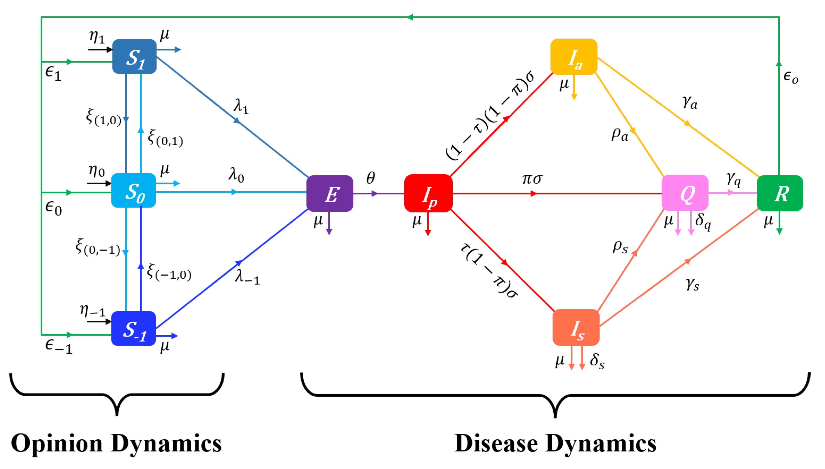
Figure 2.
Flow-chart of a UVEIQR-Opinion dynamics model showing the flow of humans between different compartments. Susceptibles are distinguished into the unvaccinated (completely susceptible) population (U), and individuals with vaccine-induced partial immunity (V), the subscripts u (unfavourable) and v (favourable) indicate attitude of U individuals toward vaccination, the subscripts indicate level of prophylactic attitude ( is the highest level of prophylactic behaviour, is the lowest level of prophylactic behaviour, and is a middle level of prophylactic behaviour); E, , , , Q and R denote respectively the exposed, the presymptomatic infectious, the asymptomatic infectious, the symptomatic infectious, the quarantined, and the recovered populations. The parameters of the model are as described in Table 1.
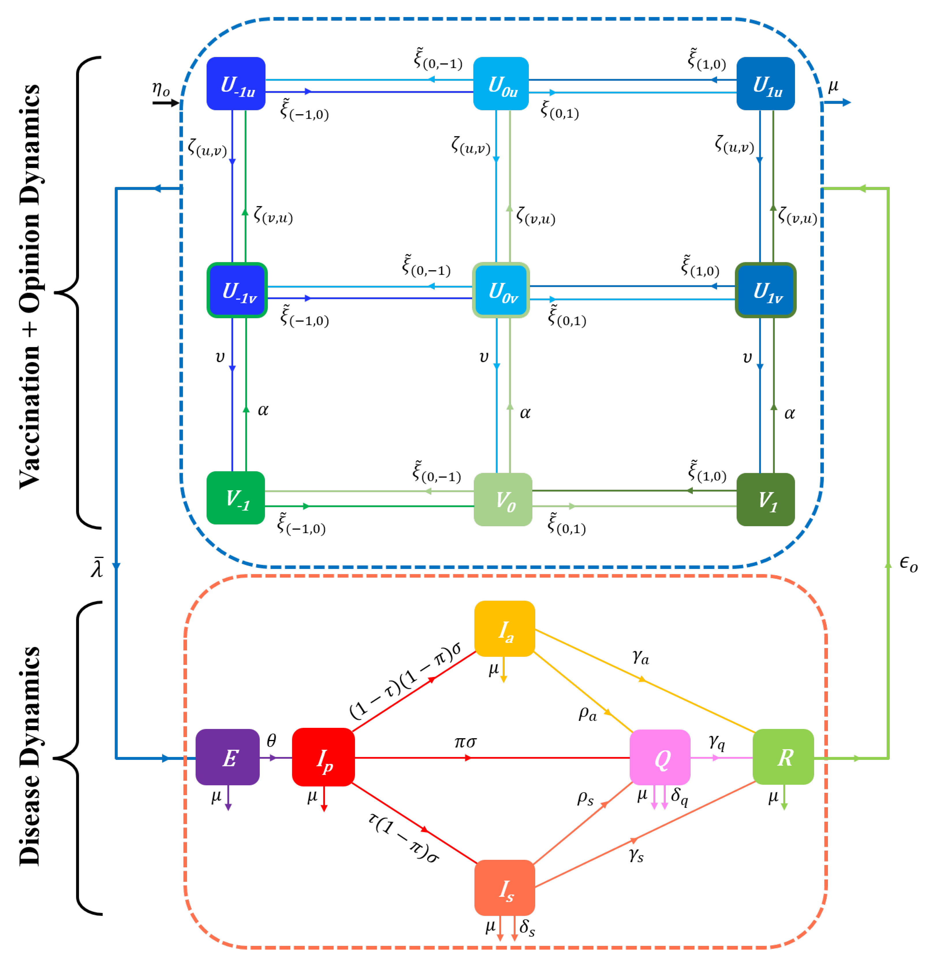

Table 1.
Description and values of parameters in the proposed models
| Parameter | Description | Values | Source |
|---|---|---|---|
| Total recruitment rate (births and net immigration) | 35,615.35 | [57] | |
| Recruitment rate of non vaccinated individuals | Assumed | ||
| Recruitment rate of vaccinated individuals () | Assumed | ||
| * | Recruitment rate of susceptibles with opinion i | ||
| * | Recruitment rate of susceptibles with opinions i and l | ||
| Natural death rate | [57] | ||
| ** | Baseline contact rate with infectious () | ||
| ** | Contact rate with an infectious with opinion i | ||
| Prophylaxy-induced infection rate reduction factor | 0.5 | [22] | |
| Exit rate from incubation state (inverse of duration) | |||
| Exit rate from presymptomatic state | |||
| Probability of early detection (presymptomatic stage) | |||
| Proportion of symptomatic infectious | |||
| ** | Detection rate of infectious () | ||
| ** | Recovery rate of infectious () | ||
| ** | Disease-related death rate of infectious () | ||
| Lost rate of disease-induced immunity | 0.011 | ||
| * | Part of recovered individuals with opinion i | ||
| * | Part of recovered individuals with opinions i and l | ||
| Vaccination rate | 0.2 | Assumed | |
| Average efficacy of available vaccines | 0.65 | Assumed | |
| Lost rate of vaccine-induced immunity | 0.015 | Assumed | |
| Baseline influence rate (when disease is not perceived) | 0.1 | [22] | |
| Skewness parameter of influence functions | 2 | Assumed | |
| Half-influence saturation constant | 0.1 | [22] |
Table notes: All parameters take nonnegative values. The recruitment rates , , , , are in “individuals per day”, the contact rates , are in “effective contacts per day”, and all other rate parameters are in “day-1”. * level of prophylactic attitude defined in Equation (3), and (unfavorable to vaccines), (favorable to vaccines, but unvaccinated), and (favorable to vaccines and vaccinated). ** (presymptomatic), a (asymptomatic), s (symptomatic), or q (quanrantined) infectious.
Disclaimer/Publisher’s Note: The statements, opinions and data contained in all publications are solely those of the individual author(s) and contributor(s) and not of MDPI and/or the editor(s). MDPI and/or the editor(s) disclaim responsibility for any injury to people or property resulting from any ideas, methods, instructions or products referred to in the content. |
© 2023 by the authors. Licensee MDPI, Basel, Switzerland. This article is an open access article distributed under the terms and conditions of the Creative Commons Attribution (CC BY) license (http://creativecommons.org/licenses/by/4.0/).
Copyright: This open access article is published under a Creative Commons CC BY 4.0 license, which permit the free download, distribution, and reuse, provided that the author and preprint are cited in any reuse.


