Option Pricing: Examples and Open Problems

1. Introduction

An option is a contract between two parties, the writer (seller) of the contract and the buyer. The buyer has the right but not the obligation to exercise the option at some time $T>0$ or even at any time at the time interval $[0,T]$. The payoff of the option that the buyer will take is an amount $H(S_1,S_2,\cdots ,S_d)$ where $H:{\mathbb{R}}_{+}^d\to {\mathbb{R}}_{+}$ and $S_1,\cdots ,S_d$ are the underlying assets. Some examples are $P_T=max\{S_T-K,0\}$ (call option), $P_T=max\{K-S_T,0\}$(put option), $P_T=max\{{max}_{t\in [0,T]}S\left(t\right)-K,0\}$ (call on maximum), $P_T=max\{S_1\left(T\right),S_2\left(T\right),K\}$ and $P_T=max\{S_1\left(T\right)-S_2\left(T\right),0\}$ (spread option) and many others.

For some options (contracts) there is the possibility of bankruptcy for the writer. For example the writer of a spread option may go bankrupt if the price of the asset $S_1$ reach high levels. The writer can buy a call option written on $S_1$ in order to eliminate that risk. However this is not the case for the call on maximum option for which the writer can buy a series of call options in order to shrink the possibility of bankruptcy but not to eliminate it.

It is clear that the writer of an option will accept to undertake the risk of selling it only for speculative reasons. The option pricing problem is equivalent to the hedging problem. There is no any option pricing model that predict the price, i.e. all the pricing models, such as the Black - Scholes and the binomial model, are in fact hedging strategies. The writer first designs a hedging strategy and then prices the option based on the amount that she need to follow that strategy. The purpose of this hedging strategy is to minimize the probability of bankruptcy and also to increase the probability of profit. Of course the competition will play a decisive role in the final sale price.

Definition 1

(Physical meaning of a price). We say that the amount Y has a physical (or realistic) meaning for the writer if

$\left(i\right)$

with this amount the writer can eliminate or at least shrink the possibility of bankruptcy

$\left(ii\right)$

and moreover with this amount has a good chance of profit.

What do we mean by "has a good chance of profit"? The exact meaning will be given by the writer herself, so in general, a different writer will price a contract differently. At [5] we have given some practical ways of doing this and will refer to them below.

One way to hedge the risk of selling an option is to built a replicating portfolio. We have two main methods to construct replicating portfolios: the first one is in discrete time and the second is in continuous time. The main representative from the first category is the binomial option pricing model, while from the second category is the Black-Scholes model. We will discuss next these two main methods and see their disadvantages.

Let us recall here the binomial option pricing model written on one asset S for the time period $[0,T]$.

Assumption 1.

Let the today price of the asset is $S_0$. We suppose that the possible values of the price at the time T are $S_T=u{S}_0$ with some probability p or $S_T=d{S}_0$ with probability $1-p$, for some numbers $u,d$.

We call $u,d$ the upward and downward rate of the future price of the asset. There are several choices for the rates in the bibliography, see for example [3,4] and [9] and the references therein.

For a specific contract, the binomial option pricing model computes the initial value of a replicating portfolio. The basic problem, however, of the binomial model is that the assumption 1 is not realistic, i.e. $\mathbb{P}(S_T=u{S}_0)=\mathbb{P}(S_T=d{S}_0)=0$ in the real world or very small! Therefore the binomial option pricing model does not produce a price with a physical meaning as we define it at definition 1. That is we are almost sure that the writer’s guess will not come true so the question is: what happens in this case concerning the value of the replicating portfolio and the payoff?

Now let us recall the Black - Scholes option pricing model, see [2] (see also [1]).

Assumption 2.

If the today price of the asset is $S_0$ then the price at time T is such that

$$\begin{array}{c}\hfill S_T=S_0+m{\int }_0^T{S}_{r}dr+\sigma {\int }_0^T{S}_{r}d{W}_r\end{array}$$

where $m,\sigma \in {\mathbb{R}}_{+}$ are some parameters specified by the writer.

Remark 1

(How the investors see the future). Every investor can assume anything she wants about the future movement of the price of the underlying asset which may differ from the above. This assumption reflects how the particular investor sees the future and for this reason (and others) the notion of a fair price of a contract does not have any meaning.

In [1] the author, in fact, proposes the price of a call or a put option to be

$$\begin{array}{c}\hfill {\mathbb{E}}_{\mathbb{P}}\left(g\left(S_T\right)\right)\end{array}$$

with $\mathbb{P}$ is the real world probability. Here $g\left(x\right)={(x-K)}^{+}$ for the call option and $g\left(x\right)={(K-x)}^{+}$ for put option. This approach have a clear physical meaning and this price can be considered as a fair price for the put option since the payoff is bounded and assuming that all investors have the same belief about the future. On the other hand the Black - Scholes model proposes the price to be

$$\begin{array}{c}\hfill {\mathbb{E}}_{\mathbb{Q}}\left(g\left(S_T\right)\right|{\mathcal{F}}_0)\end{array}$$

where $\mathbb{Q}$ is not the real world probability but an equivalent probability measure to $\mathbb{P}$. Note that ${\mathbb{E}}_{\mathbb{Q}}\left(g\left(S_T\right)\right|{\mathcal{F}}_0)=V(0,S_0)$ where $V(t,x)$ is the solution of the following famous Black - Scholes partial differential equation

$$\begin{array}{ccc}\hfill V_t(t,S)+\frac{{\sigma }^2{S}^2}{2}{V}_{SS}(t,S)+rS{V}_S(t,S)-rV(t,S)& =& 0\hfill \\ \hfill V(T,S)& =& g\left(S\right)\hfill \end{array}$$

At the first sight the above price is not intuitive at all. However, if someone go deeper to this theory understands that this price is in fact the initial value of a replicating portfolio and this explains the proposed price. Therefore, the Black - Scholes model and the binomial model have the same basic pricing principle which is based on the construction of a hedging portfolio.

So the Black - Scholes model prices a contract by the initial value of a replicating portfolio that has to be reconstructed continuously in time. Assumption 2 maybe is not the best for a specific asset but is realistic. However, the main issue of the Black - Scholes hedging strategy is the reconstruction of the replicating portfolio which is not realistic. Nobody in the real world can reconstruct such a replicating portfolio continuously in time in order to hedge the risk. To be more precise, suppose that at time t the replicating portfolio contain $a(t,S(t\left)\right)$ assets and $b(t,S(t\left)\right)$ at a bank account. At the next time that the price of the asset changes to $S(t+h)$ from $S\left(t\right)$ the number of the assets should also change instantaneously to $a(t+h,S(t+h\left)\right)$ which is impossible. Of course every pricing model via replication with reconstruction in continuous time has the same serious issue and therefore does not produce a price with a physical meaning (see definition 1).

In the spirit of [1], for general options with payoff $P_T$ (see Assumption 2.2 of [5] for example), we can define the amount ${\mathbb{E}}_{\mathbb{P}}\left(P_T\right)$ and suggest it to the writer as the possible value of the option, i.e. the average value of the payoff which has an obvious physical meaning for the writer. In [5] we have used for simplicity the Brownian motion to the assumptions concerning the payoff of a contract but is obvious that someone can use any other suitable random variable or stochastic process.

Remark 2

(Choosing a model). The trickiest part for investors is not the model that have to choose in order to fit the past data of the payoff or the asset price but the impact of recent events (or even potential future events) on the model parameters! To be more precise the main difficulty does not come from a mathematical problem but from the impossibility of predicting the future which cannot be mathematically modeled precisely. After all, for this reason there is always a possibility of profit as well as loss depending on what the investor will bet.

Note that the no arbitrage arguments (see for example [6]) does not give us a specific price for the call and put options but only a relation between them and some bounds for their prices. The situation is worse for more complicated contracts because even if we can prove some bounds for their prices the competition is maybe too low for them in order these bounds come true in the real world.

Therefore, in order to propose a pricing model via replication we should combine the realistic assumption 2 with a replication in discrete time. In [5] we have modified the binomial model in this direction.

2. The Realistic Binomial Model

As we have seen in the previous section, the writer’s guess concerning the rates $u,d$ will never come true in the real world or the probability is very low. So what happens when the true upward rate becomes bigger or less than she expected?

In [5] we have show that for the usual call and put options the writer will have a profit if the future upward rate becomes smaller of what the writer predicted or if the downward rate becomes bigger than she expected. Denote the profit of the writer of a call or put option by $\Pi$ when she is pricing by the binomial model. Let us denote the rates that she used to price the contract by $u,d$ and by $u^{*},d^{*}$ the future rates. Then the profit of these contracts is a function of $u-u^{*}$ and $d^{*}-d$, that is $\Pi :=\Pi (u-u^{*},d^{*}-d)$, and moreover this function is increasing in both variables.

Let us recall it here for the reader convenience.

Lemma 1.

Let the writer of a put or a call option with strike price K uses the one period binomial model to price it. Then she will choose the rates $d,u$ so as $u{S}_0>K$ and $d{S}_0<K$.

Proof. 

For the call option the writer will prefer to choose d so that $d{S}_0<K$ (and of course $u{S}_0>K$) where K is the strike price. Indeed, if $d{S}_0>K$ then it is easy to see that $a=1$ and $b{e}^{rT}=-K$. So, the profit $\Pi$ is as follows

$$\begin{array}{ccc}\hfill \Pi & =& a{S}_T+b{e}^{rT}-{(S_T-K)}^{+}\hfill \\ & =& S_T-K-{(S_T-K)}^{+}\hfill \end{array}$$

If $S_T>K$ then $\Pi =0$ while if $S_T\le K$ then $\Pi \le 0$, that is there is no chance for profit for the writer.

Similarly, for the put option the writer will prefer to choose u so that $u{S}_0>K$ (and of course $d{S}_0<K$). Indeed, if $u{S}_0<K$ then $a=-1$ and $b{e}^{rT}=K$ so the profit is as follows

$$\begin{array}{ccc}\hfill \Pi & =& a{S}_T+b{e}^{rT}-{(K-S_T)}^{+}\hfill \\ & =& K-S_T-{(K-S_T)}^{+}\hfill \end{array}$$

If $S_T<K$ then $\Pi =0$ while if $S_T\ge K$ then $\Pi \le 0$, that is there is no chance again for profit for the writer. □

Theorem 1

(Profit Property for Call and Put Options). Let the writer has priced a call or a put option with strike price K using the one period binomial model with rates $d,u$ which are such that $u{S}_0>K$ and $d{S}_0<K$. Then, the writer will have a profit if $\frac{S_T}{S_0}\in (d,u)$ while she will have a loss if $\frac{S_T}{S_0}\notin (d,u)$. The possible profit is bounded by the amount $\frac{(u{S}_0-K)(K-d{S}_0)}{(u-d)S_0}$ while the possible loss is unbounded.

Proof. 

We begin with the call option and recall that $a\in (0,1)$ in this case. The profit is as follows

$$\begin{array}{ccc}\hfill \Pi & =& a{S}_T+b{e}^{rT}-{(S_T-K)}^{+}\hfill \end{array}$$

If $S_T>K$ then we have that $\frac{S_T}{S_0}>d$ and that

$$\begin{array}{ccc}\hfill \Pi & =& a\left(\frac{S_T}{S_0}-u\right)S_0+au{S}_0+b{e}^{rT}-(u{S}_0-K)-\left(\frac{S_T}{S_0}-u\right)S_0\hfill \\ & =& \left(\frac{S_T}{S_0}-u\right)S_0(a-1)\hfill \end{array}$$

since $au{S}_0+b{e}^{rT}-(u{S}_0-K)=0$. Therefore in the case where $\frac{S_T}{S_0}\in (d,u)$ it holds that $\Pi >0$ while if $\frac{S_T}{S_0}>u$ it holds that $\Pi <0$. Note that if $\frac{S_T}{S_0}\to \infty$ then $\Pi \to -\infty$ as well.

If $S_T<K$ then we have that $\frac{S_T}{S_0}<u$ and that

$$\begin{array}{ccc}\hfill \Pi & =& a\left(\frac{S_T}{S_0}-d\right)S_0+ad{S}_0+b{e}^{rT}\hfill \\ & =& a\left(\frac{S_T}{S_0}-d\right)S_0\hfill \end{array}$$

since $ad{S}_0+b{e}^{rT}=0$. Again, if $\frac{S_T}{S_0}\in (d,u)$ it holds that $\Pi >0$ while if $\frac{S_T}{S_0}<d$ it holds that $\Pi <0$.

The same result holds for the put option since $a\in (-1,0)$ in this case. For both contracts it is easy to see that the possible profit is bounded by the amount

$$\begin{array}{c}\hfill \frac{(u{S}_0-K)(K-d{S}_0)}{(u-d)S_0}\end{array}$$

□

In [5] we have proposed a way of choosing $d,u$ so as to have

$$\mathbb{P}\left(\frac{S_T}{S_0}\in (d,u)\right)=p$$

for a given probability p under assumption 2. We call this as the realistic binomial model because we assume a realistic assumption for the future prices of the underlying asset and we choose the rates $d,u$ so as to fix the probability of the event $\{\frac{S_T}{S_0}\in (d,u)\}$. Of course the writer can choose the rates $d,u$ in a different way under assumption 2. For example, she can fix a $d<\frac{K}{S_0}$ and then find the $u>\frac{K}{S_0}$ such that

$$\mathbb{P}\left(\frac{S_T}{S_0}\in (d,u)\right)=p$$

for a given $p\in (0,1)$. Similarly the writer can first fix a $u>\frac{K}{S_0}$ and then find the d as above. That is, the writer bets on the event $\left\{\frac{S_T}{S_0}\in (d,u)\right\}$ when using the binomial hedging strategy for a call or a put option!

Below we give the definition of the profit property for the binomial model applied on a multi asset, in general, option. Let a contract written on d assets and let the $u_i,d_i$ are the rates guessed by the writer while by $u_i^{*},d_i^{*}$ we denote the future real rates where $i=1,\cdots ,d$. Let a replicating portfolio constructed by the (realistic) binomial model, that is let some $a_1,\cdots ,a_d,b$ such that

$$\begin{array}{c}\hfill V_T=a_1{S}_1^T+\cdots +a_d{S}_d^T+b\ge P_T\end{array}$$

assuming for simplicity the risk free rate equal to zero, where $S_i^T=u_i{S}_0$ or $S_i^T=d_i{S}_0$ and $P_T$ is the payoff in the cases where $S_i^T=u_i{S}_0$ or $S_i^T=d_i{S}_0$.

Definition 2.

We say that a replicating portfolio constructed by the (realistic) binomial model has the profit property for the contract X if the profit $\Pi =V_T-P_T$(here$V_T$and$P_T$are the real future prices for these processes) for the writer is a function of the $u_i-u_i^{*}$ and $d_i^{*}-d_i$ and is increasing in every variable.

That is the profit property is a property of a replicating portfolio that has to be reconstructed in discrete time and not a property of the realistic binomial model.

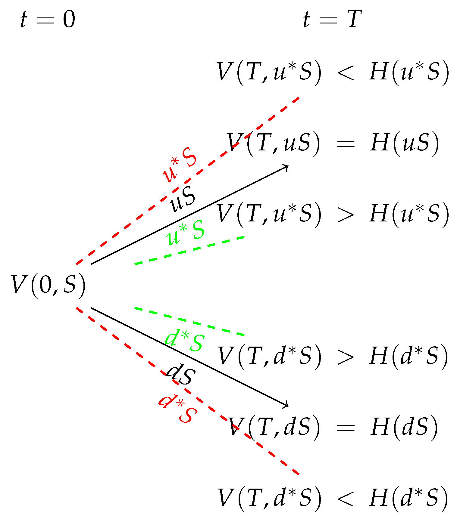
Figure 1. The replicating portfolios as constructed by the (realistic) binomial model has the profit property for both the call and the put options as we have seen in [5]. If we do not have this information then any guess of $d,u$ is meaningless because the probability to guess right is almost zero in the real world. In addition, using the realistic binomial model, we know also the probability of profit for such a replicating portfolio.

Figure 1. The replicating portfolios as constructed by the (realistic) binomial model has the profit property for both the call and the put options as we have seen in [5]. If we do not have this information then any guess of $d,u$ is meaningless because the probability to guess right is almost zero in the real world. In addition, using the realistic binomial model, we know also the probability of profit for such a replicating portfolio.

So we have combined the realistic assumption 2 for the price of the asset with the realistic reconstruction of the replicating portfolio in discrete time.

What about the well known arbitrage theorem (see for example [8]) in the binomial model setting? Let us suppose that the writer chooses $u,d$ such as $e^{rT}>u$. In this case the notion of arbitrage has no meaning because the probability of the event $\{u^{*}>e^{rT}\}$ is strictly positive!

Remark 3

(Completeness). Note that the market is incomplete under assumption 2 when the replicating portfolios has to be reconstructed in discrete time while it is complete when the replicating portfolios can be reconstructed continuously in time. However, the continuous reconstruction is not realistic so we conclude that the market is incomplete in the real world assuming 2. The best we can do in this case is to built a replicating portfolio with as high as possible probability to hedge the option. The situation is different if the underlying asset can take finite many values (due to floating point arithmetic for example) or even the quantity $U=\frac{S_T}{S_0}\in (m_T,M_T)$ for some constants $m_T,M_T$. In this case we can design a super - hedging strategy without risk. The competition (if any!) however will drive prices down in a way that the writer of the option has to undertake some risk in order to be more competitive. Therefore the writer should have a practical way to hedge and measure that risk as we have proposed by estimating the probability of profit.

Remark 4

(Binomial hedging strategy selling at the price Y). Let the writer of a call option has sell it for the amount Y and suppose that she wants to use the binomial hedging strategy using this amount. Then, she can fix a $d<\frac{K}{S_0}$ and then find a $u>\frac{K}{S_0}$ (if any!) such that

$$\begin{array}{c}\hfill Y=\frac{u{S}_0-K}{(u-d)S_0}{S}_0-\frac{(u{S}_0-K)d}{u-d}\end{array}$$

supposing zero interest rate for simplicity. Similarly, she can fix a $u>\frac{K}{S_0}$ and then find a suitable d. The same can be done for the put option.

3. A generalization of the safe price

In this section we will describe a generalization of the safe price notion by combining it with the notion of static replication. Let an option written on d assets with payoff $P_T$ at time T. The problem can be stated as follows: given some $p\in (0,1)$ and $\sigma >0$, construct a portfolio with price process $V_t$ by buying $a_i$ number of asset $S_i$, with $i=1,\cdots ,k$ at time 0 and by putting the amount b at a bank account in the following way,

$$\begin{array}{ccc}\hfill \underset{a_i,b\in {\mathbb{R}}_{+},i=1,\cdots ,k}{min}{V}_0& =& \underset{a_i,b\in {\mathbb{R}}_{+},i=1,\cdots ,k}{min}\left(\sum _{i=1}^k{a}_i{S}_i\left(0\right)+b\right)\hfill \\ \\ & \mathrm{such} \mathrm{that}& \mathbb{E}\left(P_T\right)\le \mathbb{E}\left(V_T\right)\hfill \\ & \mathrm{or}/\mathrm{and}& \mathbb{P}(P_T\le V_T)\ge p\hfill \\ & \mathrm{or}/\mathrm{and}& Var\left(V_T\right)\le \sigma \hfill \end{array}$$

or any combination of the above. This point of view has a clear physical meaning for the writer and is in fact a generalization of the safe price that we have proposed before because one can choose $a_i=0$ at the above construction. Here $k\ne d$ in general because a very important advantage of the (generalized) safe price is that we can built a replicating portfolio as above by buying assets which are, in general, different from the underlying assets! This is very useful in the case where the underlying assets can not be traded at the market.

Of course we can built a portfolio by only one asset but a diversified portfolio is more stable. An interesting problem is the following.

Problem 1.

How should the writer choose among n assets those k (k is not known in advance) to create the best possible portfolio? Can we standardize a specific mathematical methodology based on past data?

One way of course is to built a portfolio that will contain all the n assets and then simply try to choose appropriately the corresponding $a_i$, i.e. the weight of each asset.

After the construction of this replicating portfolio the writer can rebuilt it accordingly as soon as she has new information from the market.

4. Examples

Note that the model parameters are dependent also on the number of the particular N past years which have used to get the corresponding data. That is, an investor can use any N past years, not necessarily consecutive, in order to estimate the parameters of the model. A recent event has not left its mark on historical data, yet it is going to affect future ones. An investor should take this into account by increasing or decreasing the model parameters appropriately which has been calculated based on historical data.

Assumption 3.

We assume that all investors think rationally and according to their own benefit. If the competition is strong we assume that the writers will try to find the lower price for the contract but with a physical meaning for them.

4.1. Prices of the call and put options

Let us suppose that a writer want to sell a put and a call option on an underlying asset that follows the following sde

$$\begin{array}{c}\hfill S_T=40+0.01{\int }_0^T{S}_{r}dr+0.4{\int }_0^T{S}_{r}d{W}_r\end{array}$$

where $T=50$ days and the strike price is $K=41$.

Let us recall here how the writer will compute the safe price for the put option as this was proposed in [5]. For a given probability p one has to find Y such that

$$\begin{array}{c}\hfill \mathbb{P}(K-S_T\le Y)=p\end{array}$$

Under the assumption 2 about the price of the underlying asset is an easy problem to compute the safe price Y.

The price of the put option via replication (via the realistic binomial model) is about 2.8 with probability of profit 0.57 while the price without replication is 2.4 with the same probability of profit. Note that in order to construct the replicating portfolio the writer has to borrow some assets therefore under assumption 3 the writer will choose to sell without replication, i.e. at the price 2.4 or higher.

If she sell the put option at the price 2.4 then the price of the call option has to be 1.4 for the put - call parity to hold, assuming that the risk free rate is zero. Speaking about put - call parity, we can argue that taking for granted that different organizations can apply a different interest rate we find that the put - call parity is relative. At this price the probability of profit for the writer is about 0.677 for the call option without construction of a replicating portfolio. If she sell at this price the call option constructing a replicating portfolio via the realistic binomial model then the probability of profit is 0.49. In both these cases the possible loss for the writer is unbounded.

We will now describe another way of pricing a call option which we call it the $(\gamma +1)$-hedging strategy.

Theorem 2

(The $(\gamma +1)$-hedging strategy). Let a call option with strike price K and a tradable at the market underlying asset which satisfies assumption 2. Choose some $\gamma >-1$, some $p\in (0,1)$ and then a suitable $z>0$. Then selling the call option at the price

$$\begin{array}{c}\hfill Y=S_0(\gamma +1)-S_0(\gamma +1)e^{-\sigma z\sqrt{T}+(m-{\sigma }^2/2)T}\end{array}$$

the writer can have infinite possible profit if $\gamma >0$ and bounded possible loss. Moreover, the probability of profit can be greater than p choosing big enough $z>0$.

Proof. 

Indeed, the writer can borrow the amount $S_0(\gamma +1)e^{-\sigma z\sqrt{T}+(m-{\sigma }^2/2)T}$ and then buy $\gamma +1$ shares of the underlying asset.

• If $S_T>K$ then the profit $\Pi$ of the writer equals to

$$\begin{array}{ccc}\hfill \Pi & =& S_T(\gamma +1)-e^{rT}{S}_0(\gamma +1)e^{-\sigma z\sqrt{T}+(m-{\sigma }^2/2)T}-(S_T-K)\hfill \\ & =& \gamma S_T+K-e^{rT}{S}_0(\gamma +1)e^{-\sigma z\sqrt{T}+(m-{\sigma }^2/2)T}\hfill \end{array}$$

Therefore the possible profit is unbounded if $\gamma >0$ while the possible loss is unbounded if $\gamma \in (-1,0)$.

• If $S_T\le K$ then the profit $\Pi$ of the writer equals to

$$\begin{array}{c}\hfill \Pi =S_T(\gamma +1)-e^{rT}{S}_0(\gamma +1)e^{-\sigma z\sqrt{T}+(m-{\sigma }^2/2)T}\end{array}$$

Therefore the possible loss is bounded.

The probability of profit can be computed easily when $\gamma \ne 0$.

$$\begin{array}{ccc}\hfill \mathbb{P}\left(\Pi >0\right)& =& \mathbb{P}\left(\Pi >0,S_T>K\right)+\mathbb{P}\left(\Pi >0,S_T\le K\right)\hfill \\ & =& \mathbb{P}\left(S_T>max\left\{K,\frac{e^{rT}{S}_0(\gamma +1)e^{-\sigma z\sqrt{T}+(m-{\sigma }^2/2)T}-K}{\gamma }\right\}\right)\hfill \\ & & +\mathbb{P}\left(e^{rT}{S}_0{e}^{-\sigma z\sqrt{T}+(m-{\sigma }^2/2)T}\le S_T\le K\right)\hfill \end{array}$$

The above probability is a strictly increasing function of z therefore for a given $p\in (0,1)$ we can compute a suitable z such that this probability equals to p.

If $\gamma =0$ we choose a suitable z such that $e^{rT}{S}_0{e}^{-\sigma z\sqrt{T}+(m-{\sigma }^2/2)T}<K$. In this case both the possible loss and the possible profit are bounded. □

Pricing the call option using the $(1+1)$-hedging strategy and supposing for simplicity zero borrowing rate the writer can sell it at the price $1.4$. She can borrow the amount $78.6$ in order to buy two shares of the underlying asset. The potential loss is limited while the potential gain is unlimited. The resulting probability of profit equals $0.52$. The writer can design a similar hedging strategy by buying also a put option on a different strike price in order to shrink the possible loss. If the underlying asset is not tradable at the market the writer may choose another asset, if it is possible, which is tradable and behaves like the original one.

Remark 5

($(\gamma +1)$-hedging strategy selling at the price Y). Suppose that a writer of a call option sell it at the price Y and suppose that she wants to apply the $(\gamma +1)$-hedging strategy using this amount for a given γ. She can borrow the amount $S_0(\gamma +1)-Y$ and buy $(\gamma +1)$ shares of the underlying asset. The writer then, in fact, bets on the event

$$\begin{array}{c}\hfill \left\{S_0-\frac{Y}{\gamma +1}<S_T<K\right\}\bigcup \left\{S_T>max\{K,S_0+\frac{S_0-Y-K}{\gamma }\}\right\}\end{array}$$

assuming zero interest rate for simplicity. Making an assumption about the random variable $S_T$ we can estimate the probability of the above event which is the probability of profit for the writer. A similar result holds for the put option.

We can have the following hedging strategy for a call option with a tradable underlying asset which we call it the $\frac{Y}{S_0}$-hedging strategy.

Proposition 1

($\frac{Y}{S_0}$-hedging strategy). Let a call option with a tradable underlying asset which follows the geometric Brownian motion with parameters $m,\sigma$ and strike price K. If the writer sell this option at the price Y she can buy $\frac{Y}{S_0}$ shares of the asset in order the mean value and the probability of profit will be as follows

$$\begin{array}{ccc}\hfill \mathbb{E}(\Pi )& =& Y{e}^{mT}-\mathbb{E}{(S_T-K)}^{+}\hfill \\ \hfill \mathbb{P}(\Pi >0)& =& \frac{1}{\sqrt{2\pi T}}{\int }_{-\infty }^{\frac{ln\left(\frac{K}{S_0-Y}{e}^{({\sigma }^2/2-m)T}\right)}{\sigma }}{e}^{-t^2/\left(2T\right)}dt\hfill \end{array}$$

Proof. 

Indeed, the writer can buy $\frac{Y}{S_0}$ shares of the underlying asset and therefore the profit at time T is as follows,

$$\begin{array}{c}\hfill \Pi =\frac{Y}{S_0}{S}_T-{(S_T-K)}^{+}\end{array}$$

The probability of profit is as follows,

$$\begin{array}{ccc}\hfill \mathbb{P}(\Pi >0)& =& \mathbb{P}\left(\Pi >0,S_T>K\right)+\mathbb{P}(\Pi >0,S_T\le K)\hfill \\ & =& \mathbb{P}\left(S_T\left(\frac{Y}{S_0}-1\right)+K,S_T>K\right)+\mathbb{P}(S_T\le K)\hfill \end{array}$$

The result then follows easily. □

Remark 6

($\frac{Y}{S_0}$-hedging strategy selling at the price Y). Selling a call option at the price Y the writer can buy $\frac{Y}{S_0}$ shares of the underlying asset. Then, in fact, bets on the event

$$\begin{array}{c}\hfill \left\{S_T\le \frac{K}{1-\frac{Y}{S_0}}\right\}\end{array}$$

Making any suitable assumption for the random variable $S_T$ we can estimate the probability of the above event which is the probability of profit for the writer.

In the same spirit we describe the $(\gamma +1)$-hedging strategy for the put option.

Theorem 3.

Let a put option with strike price K and a tradable at the market underlying asset which satisfies assumption 2. The writer of this put option can sell it at the price

$$\begin{array}{c}\hfill Y=S_0(\gamma +1)-S_0(\gamma +1)e^{-\sigma z\sqrt{T}+(m-{\sigma }^2/2)T}\end{array}$$

for some $\gamma \in (-1,\infty )$ and for some suitable chosen by the writer $z>0$. She can invest this amount in a way that will have unbounded possible profit and bounded possible loss for a given probability of profit.

Proof. 

Indeed, she can buy $\gamma +1$ shares of the underlying asset borrowing the amount $S_0(\gamma +1)e^{-\sigma z\sqrt{T}+(m-{\sigma }^2/2)T}$. The profit at time T will be

$$\begin{array}{c}\hfill \Pi =S_T(\gamma +1)-e^{rT}{S}_0(\gamma +1)e^{-\sigma z\sqrt{T}+(m-{\sigma }^2/2)T}-{(K-S_T)}^{+}\end{array}$$

where r is the borrowing rate. It is clear that if $S_T>K$ then the possible profit for the writer is unbounded while if $S_T<K$ then the possible loss for the writer is bounded by the amount $e^{rT}{S}_0{e}^{-\sigma z\sqrt{T}+(m-{\sigma }^2/2)T}+K$.

We can compute a suitable z in order to have a desired probability of profit as we did at the call option case. □

Using the $(0+1)$-hedging strategy the writer can sell the put option at the price $2.4$ having $0.52$ probability of profit assuming zero borrowing rate for simplicity. The advantage however is that the possible profit is unbounded.

A useful criterion is to compute the mean value of the profit of each pricing method.

Corollary 1.

Let a call option with strike price K and suppose that the underlying asset satisfies the geometric Brownian motion with parameters $m,\sigma$. Then the mean values of the profits are

$$\begin{array}{ccc}\hfill \mathbb{E}\left({\Pi }_{rb}\right)& =& a{S}_0{e}^{mT}+b-\mathbb{E}{(S_T-K)}^{+}(realistic binomial model)\hfill \\ \hfill \mathbb{E}\left({\Pi }_{sp}\right)& =& S_0{e}^{\sigma z_{sp}\sqrt{T}+(m-{\sigma }^2/2)T}-K-\mathbb{E}{(S_T-K)}^{+}(safe price)\hfill \\ \hfill \mathbb{E}\left({\Pi }_{\gamma +1}\right)& =& (\gamma +1)S_0\left(e^{mT}-e^{-\sigma z_{\gamma }\sqrt{T}+(m-{\sigma }^2/2)T}\right)\hfill \\ & & -\mathbb{E}{(S_T-K)}^{+}\left(\right(\gamma +1)-hedging strategy)\hfill \end{array}$$

where $a=\frac{u{S}_0-K}{(u-d)S_0}$ and $b=-\frac{(u{S}_0-K)d}{(u-d)}$ supposing zero interest rate for simplicity. Here the rates $u,d$ are some suitable rates in order the writer has a predefined probability of profit using the realistic binomial option pricing model.

Of course we can have similar computations for the $\mathbb{E}(\Pi |\Pi <0)$, $\mathbb{E}(\Pi |\Pi >0)$, $Var(\Pi )$ and others.

Table 1. We compare the four hedging strategies by computing the probability of profit and the mean value of profit selling the call option at the same price $Y=2.0$. Note that at the safe price hedging strategy, the $\frac{Y}{S_0}$-hedging strategy and the realistic binomial model hedging strategy the possible loss is unbounded while for the $(0.01+1)$-hedging strategy the possible loss is bounded and the possible profit is unbounded! Selling at this price and using the hedging strategy proposed by the Black-Scholes model is impossible!

$\mathit{Y}=2.0$	Probability of profit	Mean value of profit	Loss and profit
Safe price hedging strategy	$0.71$	$0.05$	Bounded profit but unbounded loss
$\frac{Y}{S_0}$-hedging strategy	$0.71$	$0.05$	Bounded profit but unbounded loss
Realistic binomial model	$0.61$	$0.09$	Bounded profit but unbounded loss
$(0.01+1)$-hedging strategy	$0.6$	$0.09$	Bounded loss and unbounded profit

Table 1. We compare the four hedging strategies by computing the probability of profit and the mean value of profit selling the call option at the same price $Y=2.0$. Note that at the safe price hedging strategy, the $\frac{Y}{S_0}$-hedging strategy and the realistic binomial model hedging strategy the possible loss is unbounded while for the $(0.01+1)$-hedging strategy the possible loss is bounded and the possible profit is unbounded! Selling at this price and using the hedging strategy proposed by the Black-Scholes model is impossible!

$\mathit{Y}=2.0$	Probability of profit	Mean value of profit	Loss and profit
Safe price hedging strategy	$0.71$	$0.05$	Bounded profit but unbounded loss
$\frac{Y}{S_0}$-hedging strategy	$0.71$	$0.05$	Bounded profit but unbounded loss
Realistic binomial model	$0.61$	$0.09$	Bounded profit but unbounded loss
$(0.01+1)$-hedging strategy	$0.6$	$0.09$	Bounded loss and unbounded profit

Let us suppose that the writer sell the put option at the price $Y=3.1$. Then the probability of profit without replication is about $0.62$. But in this case the writer can construct a replicating portfolio without borrowing assets i.e. with $a=0.05$ and $b=1$. In this case the writer will have a (possible unbounded!) profit if $\frac{S_T}{S_0}\ge 0.95$ and the probability of this event is about $0.52$.

The Black - Scholes model price for the put option is about $2.91$, constructing a (impossible!) replicating portfolio, while ${\mathbb{E}}_{\mathbb{P}}\left({(K-S_T)}^{+}\right)=2.89$ under assumption 2. Here

$$\begin{array}{c}\hfill {\mathbb{E}}_{\mathbb{P}}\left({(K-S_T)}^{+}\right)=\frac{1}{\sqrt{2\pi T}}{\int }_{-\infty }^M(K-S_0{e}^{(m-{\sigma }^2/2)T+\sigma x})e^{-x^2/\left(2T\right)}dx\end{array}$$

with $M=({\sigma }^2/2-m)\frac{T}{\sigma }+\frac{lnK-ln{S}_0}{\sigma }$. In the Black - Scholes setting one should borrow assets, assuming that can indeed rebuilt the portfolio continuously in time, while the physical meaning of the mean value of the payoff is clear without replication.

Suppose now that the underlying asset can not be traded at the market. The writer choose another asset which follows the following stochastic differential equation

$$\begin{array}{c}\hfill {\widehat{S}}_t=2+{\int }_0^{t}0.02{\widehat{S}}_{s}ds+{\int }_0^{t}0.3{\widehat{S}}_{s}d{\widehat{W}}_s,t\in [0,T]\end{array}$$

where ${\widehat{W}}_t$ is a Brownian motion independent (in general) of $W_t$. The writer decide to construct a portfolio containing the asset $\widehat{S}$ which can be traded at the market. One way to choose such an asset is to choose between those having a high drift parameter and small diffusion parameter (i.e. volatility). The portfolio will contain $a\in {\mathbb{R}}_{+}$ number of the asset $\widehat{S}$ and $b\in {\mathbb{R}}_{+}$ at the bank account. The writer, in order to price the contract, choose to solve the following minimization problem

$$\begin{array}{c}\hfill \underset{a,b\in {\mathbb{R}}_{+}}{min}(a{\widehat{S}}_0+b)\\ \hfill \mathbb{E}\left(P_T\right)=\mathbb{E}\left(V_T\right)\end{array}$$

where $V_T=a{\widehat{S}}_T+b$ and therefore $\mathbb{E}\left(V_T\right)=2a{e}^{0.02T}+b$. Recall that $\mathbb{E}\left(P_T\right)=2.89$ so from the equality $\mathbb{E}\left(P_T\right)=\mathbb{E}\left(V_T\right)$ we deduce that $b=max\{2.89-2a{e}^{0.02T},0\}$. That is we have to minimize the quantity

$$\begin{array}{c}\hfill 2a+max\{2.89-2a{e}^{0.02T},0\}\end{array}$$

for $a\in {\mathbb{R}}_{+}$. It follows that the minimum is for $a=\frac{2.89}{2e^{0.02·50/360}}=2.005$ and $b=0$ and consequently the suggested price is $2.005·2=2.87$ recalling that we assumed that the interest rate is zero.

Recalling that the price $Y=1.4$ is the value which is such that $\mathbb{P}(P_T\le Y)=0.5$, the writer can construct a portfolio with $\mathbb{P}(V_T\ge Y)=0.5$ where $V_T=a{\widehat{S}}_T+b$. That is the probability $\mathbb{P}(P_T\le Y\le V_T)=\mathbb{P}(V_T\ge Y)\mathbb{P}(P_T\le Y)$. We can work of course directly on the probability $\mathbb{P}(P_T\le V_T)$ but with a different result. It follows that the minimum portfolio is that with $a=\frac{Y}{{\widehat{S}}_0}{e}^{({\widehat{\sigma }}^2/2-\widehat{m})T}$ and $b=0$. Here $\widehat{\sigma }$ and $\widehat{m}$ are the parameters of ${\widehat{S}}_t$. If the asset has small volatility, say $\widehat{\sigma }=0.001$ and high drift term, say $\widehat{m}=0.01$, then the value $a{\widehat{S}}_0+b=1.39$ can be considered as a price for this contract with a clear physical meaning.

If the competition is strong the writers will try to find the lower price for the contract but with a physical meaning for them. Assuming that the competition is strong, the most likely price for the put option is about $1.4$ for which both the buyer and the writer have the same probability of profit (without replication), i.e. $0.5$, while for both of them the possible profit is bounded. That is the notion of the fair price has a meaning only if both the buyer and the seller have bounded possible profits and does not come necessarily by a replicating portfolio! Of course this is true only if all the investors have the same beliefs about the future. The price of the call option then has to be 0.4 in order the put - call parity holds. The probability of profit is about $0.617$ for this price, that is far enough from the probability $0.5$. The above holds in the case where all the investors have the same belief about the future!

Remark 7

(Arbitrage free prices). The put - call parity, which holds due to the arbitrageurs, is a relation between the prices of the call and put options which does not give us a specific price for these options. In the real world does not hold because of the transaction costs and maybe because of the lack of arbitrageurs! Supposing zero transaction costs the arbitrageurs (if any) will push high prices down and low prices up. Concerning all the above hedging strategies, this will happen by choosing suitable probability of profit.

One can construct infinitely many pricing models for the call and put options which preserve not only the put - call parity formula but also the bounds for their prices. It is well known that the prices of the call and put option should satisfy the following inequalities in order to be free of arbitrage,

$$\begin{array}{c}\hfill S_0-K<C<S_0\\ \hfill K-S_0<P<K\\ \hfill C-P=S_0-K\end{array}$$

where C is the price of the call option, P is the price of the put option, K is the strike price assuming zero interest rate for simplicity. Then one can price the options as follows

$$\begin{array}{c}\hfill C=S_0-a,a\in (0,K)\\ \hfill P=K-b,b\in (0,S_0)\end{array}$$

We should choose $a=b\in \left(0,min\{S_0,K\}\right)$ so that the put - call parity holds and we have infinite ways to do this. That is, for any $a\in \left(0,min\{S_0,K\}\right)$ the prices $C=S_0-a$ and $P=K-a$ are arbitrage free! In order to meet the definition 1 we should describe what the writer can do with this amount. For example, for the call option one suitable hedging strategy is the $(\gamma +1)$-hedging strategy in which the writer can borrow the amount $S_0\gamma +a$ in order to buy $\gamma +1$ shares of the underlying asset. Under this hedging strategy the possible loss is bounded by the amount $S_0\gamma +a$ while the possible profit is unlimited. We can apply also the $(\gamma +1)$-hedging strategy for the put option. Therefore we have just presented infinitely many ways to produce arbitrage free prices for the call and put options and at the same time we have designed also a practical hedging strategy for each of them! The Black - Scholes hedging strategy propose arbitrage free prices but no practical hedging strategies!

If the writer want to estimate the probability of profit or the mean value of profit she should make an assumption about the price of the underlying asset.

It will be very interesting if we can find other, different from the above, realistic ways to price these options.

Consider now the case of a put option in which the Black - Scholes price equal $X_1$, the safe price equal $X_2$ and the average value of the payoff equal $X_3$ with $X_3,X_2>X_1$. If the writer sell the option at the price $X_1$ she should construct the replicating portfolio in order to have a meaning for her but this is not possible in practice. Selling the option either at the price $X_2$ or $X_3$ then the physical meaning is clear and therefore the competition will force the price of this contract to be $min\{X_2,X_3\}$.

Problem 2.

What is the probability of profit for a call option using the n period realistic binomial model?

A partial answer is the following theorem. By q we denote the probability $q=\{\frac{S_{n+1}}{S_n}>1\}$ which we have computed in [5].

Theorem 4.

Let a call option with strike price K. Suppose that the writer has priced it by using the n - period realistic binomial model under assumption 2 with

$$\begin{array}{c}\hfill u=e^{\sigma z_p\sqrt{\frac{T}{n}}+(m-{\sigma }^2/2)\frac{T}{n}},d=e^{-\sigma z_p\sqrt{\frac{T}{n}}+(m-{\sigma }^2/2)\frac{T}{n}}\end{array}$$

Here $z_p$ is such that ${\displaystyle \frac{1}{\sqrt{2\pi \frac{T}{n}}}{\int }_{-z_p\frac{T}{n}}^{z_p\frac{T}{n}}{e}^{\frac{-t^2}{2\frac{T}{n}}}dt=p}$ with p chosen by the writer and is such that $u>1$ and $d<1$. Then the probability of profit at the last step $\mathbb{P}(\Pi \ge 0)\to 0$as $n\to \infty$ assuming that the writer construct the replicating portfolio as she design it at first by placing or withdrawing corresponding amounts of money.

Proof. 

Let’s assume that the writer constructs the replicated portfolio as she originally designed it by placing or withdrawing corresponding amounts of money. This is because the asset price will almost never receive the appraised values.

The profit at time T is

$$\begin{array}{ccc}\hfill \Pi & =& a_{n-1}U{S}_0+b_{n-1}-H\left(U{S}_0\right)\hfill \end{array}$$

where $H\left(x\right)={(x-K)}^{+}$ and $a_{n-1},b_{n-1}$ are such that $a_{n-1}u{S}_{n-1}+b_{n-1}=H\left(u{S}_{n-1}\right)$ and $a_{n-1}d{S}_{n-1}+b_{n-1}=H\left(d{S}_{n-1}\right)$. Finally $U=e^{\sigma W_T+(m-{\sigma }^2/2)T}$ is the real value of the asset at time T after some upward and downward jumps. From now on we will denote by $a,b$ the $a_{n-1}$ and $b_{n-1}$ and by $S_{n-1}$ the estimated value of the asset after the same upward and downward jumps.

Suppose that $d{S}_{n-1}<U{S}_0<K$. Then the profit is

$$\begin{array}{ccc}\hfill \Pi & =& aU{S}_0+b-H\left(U{S}_0\right)\hfill \\ & =& a(U{S}_0-d{S}_{n-1})+H\left(d{S}_{n-1}\right)-H\left(U{S}_0\right)\hfill \\ & =& (U{S}_0-d{S}_{n-1})\left(a-\frac{H\left(U{S}_0\right)-H\left(d{S}_{n-1}\right)}{U{S}_0-d{S}_{n-1}}\right)\hfill \end{array}$$

and it follows that $\Pi \ge 0$. If $U{S}_0<d{S}_{n-1}<K$ then $\Pi \le 0$ and if $U{S}_0<K<d{S}_{n-1}$ then $\Pi \le 0$ because $a=1$ and $\frac{H\left(U{S}_0\right)-H\left(d{S}_{n-1}\right)}{U{S}_0-d{S}_{n-1}}\le 1$. Similarly, if $K<U{S}_0$, it follows that $\Pi \ge 0$ if $U{S}_0\le u{S}_{n-1}$ and $\Pi \le 0$ if $U{S}_0\ge u{S}_{n-1}$.

Therefore the profit is no-negative in the case where $d{S}_{n-1}\le U{S}_0\le u{S}_{n-1}$ and non positive otherwise.

The probability of profit is then

$$\begin{array}{ccc}\hfill \mathbb{P}\left(d{S}_{n-1}\le U{S}_0\le u{S}_{n-1}\right)& =& \\ \hfill \sum _{k=0}^{n-1}{q}^k{(1-q)}^{n-1-k}\mathbb{P}(u^k{d}^{n-1-k}\left(d{S}_0\right)\le U{S}_0\le u^k{d}^{n-1-k}\left(u{S}_0\right))\end{array}$$

But

$$\begin{array}{ccc}& & \mathbb{P}(u^k{d}^{n-1-k}\left(d{S}_0\right)\le U{S}_0\le u^k{d}^{n-1-k}\left(u{S}_0\right))\hfill \\ & =& \mathbb{P}\left(e^{\sigma z_p\sqrt{\frac{T}{n}}(2k-n)+(m-{\sigma }^2/2)T}\le e^{\sigma W_T+(m-{\sigma }^2/2)T}\le e^{\sigma z_p\sqrt{\frac{T}{n}}(2k+2-n)+(m-{\sigma }^2/2)T}\right)\hfill \\ & =& \mathbb{P}\left(\sigma z_p\sqrt{\frac{T}{n}}(2k-n)\le \sigma W_T\le \sigma z_p\sqrt{\frac{T}{n}}(2k+2-n)\right)\hfill \\ & =& \frac{1}{\sqrt{2\pi T}}{\int }_{\sigma z_p\sqrt{\frac{T}{n}}(2k-n)}^{\sigma z_p\sqrt{\frac{T}{n}}(2k+2-n)}{e}^{-t^2/\left(2T\right)}dt\hfill \\ & \le & \frac{2\sigma z_p}{\sqrt{2\pi n}}\hfill \end{array}$$

Therefore

$$\begin{array}{c}\hfill \mathbb{P}\left(d{S}_{n-1}\le U{S}_0\le u{S}_{n-1}\right)\le \frac{2\sigma z_p}{\sqrt{2\pi n}}\sum _{k=0}^{n-1}{q}^k{(1-q)}^{n-1-k}=\frac{2\sigma z_p}{(1-q)\sqrt{2\pi n}}\end{array}$$

Therefore, the probability of profit at the last step is getting smaller as $n\to \infty$ and of course that means that the probability of loss is getting bigger. □

Problem 3.

At time k, knowing the actual path of the asset’s price until that time, what the writer can do concerning the hedging strategy in order to increase the profit and the probability of profit? What about other types of options written on one asset, for example path dependent options?

Remark 8.

Intuitively speaking, the realistic binomial model can be used for one period without troubles while for n periods there are open questions concerning the hedging strategy and how should be modified by the writer given the actual path of the asset’s price. Theorem 4 together with problem 3 can be considered as a recommendation for static hedging only and in particular for only one time. The situation for more complex options seems to be worse.

Example 1.

Suppose that the underlying asset today price is $S_0=1$ and the strike price is $K=1$. Suppose that the writer prices a call option using the two period realistic binomial model choosing $u=1.2$ and $d=0.8$. It follows that the initial price of the replicating portfolio is $V_0=0.11$.

Suppose now that the first jump of the asset is upward but with $u^{*}=1.4$. Then, the replicating portfolio has the price $V_1^{u^{*}}=a_0{u}^{*}{S}_0+b_0=0.33$. At time $n=1$ the writer should reconstruct the replicating portfolio and chooses to stay at the $a_1^u,b_1^u$ as these have computed at first. To do so, the writer has to put the amount $0.4033-0.33$, which is such that $a_1^u{u}^{*}{S}_0+b_1^u=0.4033$. Supposing that the next jump is upward with $u=1.2$ we have that the writer profit is

$$\begin{array}{c}\hfill a_1^u{u}^{*}u{S}_0+b_1^u-max(u^{*}u{S}_0-K,0)+0.33-0.4033=-0.0933\end{array}$$

Is there another reconstruction which will drive the writer to a less loss or even to a positive profit?

At the time $n=1$ new information from the market has arrived so the writer can use these information to make a better guess of the future. At time $n=1$ the value of the replicating portfolio is $0.33$ and the writer decides to construct the portfolio $(a,b)$ with $a=2$ and $b=-2.47$ using this amount of money. Suppose that at the time $n=2$ the asset goes upward with $u=1.3$, that is the value of the asset at time $n=2$ is $S_2^{uu}=1\times 1.4\times 1.3=1.82$ while the value of the portfolio is $2\times 1.4\times 1.3-2.47=1.17$. The payoff in this case is $1.4\times 1.3-1=1.82-1=0.82$. Therefore the writer make a profit in this case. If the writer deems it appropriate, she can reconstruct the portfolio more often or less frequently than she originally planned.

In short, it may be preferable (in a multi-period binomial model) for the seller to reconstruct the portfolio not as originally designed but using new information as well as making new guesses.

Remark 9

(Conclusions that are independent of the assumptions). We have assumed that the price of the underlying asset follows the geometric Brownian motion with parameters $m,\sigma$. Some conclusions depends strongly on this assumption but there are some other which are independent! For example, concerning the realistic binomial hedging strategy for the call and put options the conclusion that the writer will have a profit if $\frac{S_T}{S_0}\in (d,u)$ is independent of the assumption about the price of the underlying. The conclusion, however, concerning the probability of this event depends on this assumption. Concerning the $(\gamma +1)$-hedging strategy we have concluded that if $\gamma >0$ then the writer will have unlimited possible profit and bounded possible loss and the bound of loss equals to the amount which the writer have borrowed. Again, the probability of profit and the mean value of profit depends on the assumption that we will make about the price of the underlying asset. For the safe price the conclusion that the writer will have a profit if $S_T<K$ (concerning the call option) is independent of the assumption while the probability of profit of course depends on this. The same hold about the $\frac{Y}{S_0}$-hedging strategy. Here the Black-Scholes hedging strategy has again a disadvantage. It is seems that there is no conclusion which is independent of the assumption concerning the price of the underlying asset even if we could indeed construct this portfolio in the real world!

Hedging strategy	Conclusions independent of the assumption 2
Black-Scholes hedging strategy	None!
$\frac{Y}{S_0}$-hedging strategy and Safe price hedging strategy	Profit if $S_T<K$ for the call option while for the put option there will be a profit if $S_T>K$. The possible loss is unlimited while the possible profit is bounded.
Binomial model	Profit if $\frac{S_T}{S_0}\in (d,u)$ and loss otherwise. The possible loss is unlimited while the possible profit is bounded.
$(\gamma +1)$-hedging strategy	Unlimited possible profit and bounded possible loss if $\gamma >0$!

Therefore any conclusion which is independent of the assumption 2 can be used safely by the writer in order to make a decision while any conclusion that depends on this assumption do not.

Summing up, the well known binomial option pricing model has no meaning because the writer’s guess will not come true in the real world and in addition the writer does not know anything about a possible profit and what is the probability of profit. On the other hand, concerning the realistic binomial model, given that the corresponding replicating portfolio has the profit property, the writer knows what is the probability of profit and in which cases will have a profit, at least for the one period model. Pricing by the Black - Scholes model the problem is that the writer can not built the replicating portfolio in order to hedge the risk and therefore nobody will price a contract in this way.

4.2. An option written on two underlying assets

Let two assets $S_1,S_2$ that follows the following sdes

$$\begin{array}{ccc}\hfill S_1\left(T\right)& =& 0.98+0.001{\int }_0^T{S}_1\left(r\right)dr+0.5{\int }_0^T{S}_1\left(r\right)d{W}_r^1\hfill \\ \hfill S_2\left(T\right)& =& 0.99-0.02{\int }_0^T{S}_2\left(r\right)dr+0.6{\int }_0^T{S}_2\left(r\right)d{W}_r^2\hfill \end{array}$$

where $T=50$ days and $W_t^1,W_t^2$ are independent (in general) Brownian motions. Let $K=0.99$ and consider the option that pays $P_T=max\{S_1,S_2,K\}$ at the time T. The writer of the option computes a replicating portfolio via the realistic binomial model with probability of profit $p=0.7$ and finds that she should buy $a_1=0.47$ shares of the $S_1$ asset, $a_2=0.49$ shares of the $S_2$ asset and $b=0.23$ at the bank account assuming zero risk free rate. To be more precise the probability $p=0.7$ is not the probability of profit but the probability of the event $\{\frac{S_i^T}{S_i^0}\in (d_i,u_i)\}$. The probability of profit in this case is not so easy to compute as in the call and put options. The initial value of this portfolio is $V_0=1.18$. It is easy to prove that this replicating portfolio has the profit property. In fact any replicating portfolio with $a_i\in [0,1]$ has the profit property concerning this type of contract. That is we can find the minimum replicating portfolio for $a_i\in [0,1]$ therefore this portfolio will have the profit property. The writer, if she wants to be more competitive, she will try to find the replicating portfolio with the profit property having the minimum initial value. At this example the notion of the fair value does not have any sense because the possible profit of the buyer is unbounded while the possible profit for the writer is bounded.

The writer computes also the safe price under the same hypotheses as above and finds that this price is $Y=1.09$ with the same probability p but without replication. Let us recall here how to compute the safe price under the above assumptions as we have proposed in [5]. For a given probability p we find the prices $S_1^Y$ and $S_2^Y$ so that

$$\begin{array}{ccc}\hfill \mathbb{P}(S_1^T\le S_1^Y)& =& p\hfill \\ \hfill \mathbb{P}(S_2^T\le S_2^Y)& =& p\hfill \end{array}$$

Then the safe price is $Y=max\{S_1^Y,S_2^Y,K\}$.

The writer has to buy some call options in order to eliminate the risk of bankruptcy. At the first case, i.e. with the construction of the replicating portfolio, should buy $(1-a_1)$ calls with underlying asset $S_1$ for some strike price $K_1$ and $(1-a_2)$ calls with underlying asset $S_2$ for some strike price $K_2$. At the second case she should buy one call per asset.

The final price will be computed after the estimation of the transactions costs for the replication and the cost of the call options, i.e. in the first case the price will be $Y=1.18+(1-a_1)C(S_1,K_1)+(1-a_2)C(S_2,K_2)+T$ where $C(·,·)$ are the call options and T the transactions costs. At the second case the final price will be $U=1.09+C(S_1,K_1)+C(S_2,K_2)+T$.

We give below the definition of the binomial replicating portfolio for a contract with payoff $P_T(S_1,S_2,\cdots ,S_d)$ where $S_1,S_2,\cdots ,S_d$ are the underlying assets.

Definition 3.

Let $u_i,d_i$ for $i=1,\cdots ,d$ be given. We say that a portfolio $V_0=a_1{S}_1^0+\cdots +a_d{S}_d^0+b$ is a binomial replicating portfolio for the contract with payoff $P_T(S_1,S_2,\cdots ,S_d)$ if

$$\begin{array}{c}\hfill a_1{v}_1{S}_1^0+\cdots +a_d{v}_d{S}_d^0+b\ge P_T(v_1{S}_1^0,\cdots ,v_d{S}_d^0)\end{array}$$

where $v_i=d_i$ or $v_i=u_i$ for $i=1,\cdots ,d$ assuming zero interest rate.

We can now easily prove the following proposition concerning the profit property of the binomial replicating portfolio.

Proposition 2.

Let a replicating portfolio for the contract with payoff $P_T=max\{S_1^T,S_2^T,K\}$ for some $K>0$ with $u_i{S}_i^0>K$ and $d_i{S}_i^0<K$ for $i=1,2$ and $a_i\in [0,1]$. Then the writer will have a profit using the binomial hedging strategy at least on the event

$$\begin{array}{c}\hfill \left\{\frac{S_1^T}{S_1^0}\in (d_1,u_1)\right\}\bigcap \left\{\frac{S_2^T}{S_2^0}\in (d_2,u_2)\right\}\end{array}$$

Proof. 

The payoff can be $P_T=S_1^T$, $P_T=S_2^T$ or $P_T=K$. We will prove in either case that the profit is nonnegative at the event

$$\begin{array}{c}\hfill \left\{\frac{S_1^T}{S_1^0}\in (d_1,u_1)\right\}\bigcap \left\{\frac{S_2^T}{S_2^0}\in (d_2,u_2)\right\}\end{array}$$

$\left(i\right)$

We suppose that $P_T=S_1^T$. Then the profit $\Pi$ is as follows, denoting by $v_i=\frac{S_i^T}{S_i^0}$,

$$\begin{array}{ccc}\hfill \Pi & =& a_1{v}_1{S}_1^0+a_2{v}_2{S}_2^0+b-v_1{S}_1^0\hfill \\ & =& a_1{u}_1{S}_1^0-a_1{u}_1{S}_1^0+a_1{v}_1{S}_1^0+a_2{d}_2{S}_2^0-a_2{d}_2{S}_2^0+a_2{v}_2{S}_2^0+b-v_1{S}_1^0\hfill \\ & \ge & S_1^0(u_1-v_1)(1-a_1)+a_2{S}_2^0(v_2-d_2)\hfill \\ & \ge & 0\hfill \end{array}$$

$\left(ii\right)$

We suppose that $P_T=S_2^T$. The proof is similar to the previous case.

$\left(iii\right)$

We suppose that $P_T=K$. Then the profit $\Pi$ is as follows, denoting by $v_i=\frac{S_i^T}{S_i^0}$,

$$\begin{array}{ccc}\hfill \Pi & =& a_1{v}_1{S}_1^0+a_2{v}_2{S}_2^0+b-K\hfill \\ & =& a_1{d}_1{S}_1^0-a_1{d}_1{S}_1^0+a_1{v}_1{S}_1^0+a_2{d}_2{S}_2^0-a_2{d}_2{S}_2^0+a_2{v}_2{S}_2^0+b-K\hfill \\ & \ge & a_1{S}_1^0(v_1-d_1)+a_2{S}_2^0(v_2-d_2)\hfill \\ & \ge & 0\hfill \end{array}$$

□

Remark 10

(Hedging strategies for the ${\mathbf{P}}_{\mathbf{t}}=max\{{\mathbf{S}}_{\mathbf{1}}^{\mathbf{T}},{\mathbf{S}}_{\mathbf{2}}^{\mathbf{T}},\mathbf{K}\}$). One hedging strategy for the contract with payoff $P_T=max\{S_1^T,S_2^T,K\}$ is to first buy call options (in order to eliminate the risk of bankruptcy) with underlying assets $S_1,S_2$ while the remaining amount can be used for the binomial hedging strategy. The writer in this case bets, at least, on the event $\left\{\frac{S_1^T}{S_1^0}\in (d_1,u_1)\right\}\bigcap \left\{\frac{S_2^T}{S_2^0}\in (d_2,u_2)\right\}$. The writer can borrow an amount if she want to increase the probability of profit.

The $(\gamma +1)$-hedging strategy can be used also to hedge this type of contract. For example, the writer can sell this option at the price Y and then borrow the amount $S_1^0({\gamma }_1+1)+S_2^0({\gamma }_2+1)-Y$ in order to buy${\gamma }_1+1$shares of$S_1$and ${\gamma }_2+1$shares of$S_2$. Then the profit for the writer equal to

$$\begin{array}{c}\hfill \Pi =S_1^T({\gamma }_1+1)+S_2^T({\gamma }_2+1)-S_1^0({\gamma }_1+1)-S_2^0({\gamma }_2+1)+Y-P_T\end{array}$$

Similar as before conclusions can be made about the event on which the writer will have a profit and moreover if ${\gamma }_i>0$ for $i=1,2$ then there is no risk for bankruptcy.

As we have seen in [5] there is also another way to compute a price for some given probability of profit for the writer. The writer can assume that $P_T=max\{X_T,K\}$ for a stochastic process $X_t$ suitably chosen by her. This point of view is very useful in the case where the underlying assets are not tradable. In fact the same assumption can be done by the buyer in order to estimate the probability of profit for her, however, the way that the two parties estimates the probability of profit are in general different from each other.

After the decision of the writer about the price (say U) of this option the buyer can compute also the probability of profit for her buying at this price. This probability is more likely to be under $1/2$ but this is acceptable by the buyer because the profit is unbounded from above. Recall that the call options will pay this extra difference.

Problem 4.

Does the (realistic) binomial model can produce a replicating portfolio with the profit property for any known contract? Let a replicating portfolio $(a_1^{*},a_2^{*},\cdots ,a_d^{*},b^{*})$ such that

$$V_0=a_1^{*}{S}_1+a_2^{*}{S}_2+\cdots +a_d^{*}{S}_d{b}^{*}=\underset{a_1,a_2,\cdots ,a_d,b\in \mathbb{R}}{min}(a_1{S}_1+a_2{S}_2+\cdots +a_d{S}_d+b)$$

and the minimum is taken over all the replicating portfolios. The question is: does this portfolio has the profit property for a specific contract? If yes, what is the probability of profit for the writer?

4.3. A spread option

In this subsection we will study a spread option with payoff $P_T=max\{S_1-S_2,0\}$. We will compute a replicating portfolio by using the realistic binomial model and this portfolio will have the profit property and we can prove that using similar arguments as before. Therefore the writer will know in which cases she will have a profit. Moreover, we will compute the safe price, i.e. a price without a replicating portfolio. The final price will be decided by the writer after the computation of the call options in order to eliminate the risk of bankruptcy and of course the transaction costs. On the other hand, the buyer has the ability to estimate the profit probability for her buying at this price.

Let two assets $S_1,S_2$ that follows the following sdes

$$\begin{array}{ccc}\hfill S_1\left(T\right)& =& 0.98+0.001{\int }_0^T{S}_1\left(r\right)dr+0.5{\int }_0^T{S}_1\left(r\right)d{W}_r^1\hfill \\ \hfill S_2\left(T\right)& =& 0.99-0.02{\int }_0^T{S}_2\left(r\right)dr+0.6{\int }_0^T{S}_2\left(r\right)d{W}_r^2\hfill \end{array}$$

where $T=50$ days. The writer finds a replicating portfolio with $a_1=1.0$, $a_2=-0.06$ and $b=-0.714$. This portfolio clearly has the profit property using the realistic binomial model with $p=0.7$. The initial value of this portfolio is $V_0=0.19$. We compute also the safe price with probability $p=0.7$ and the price is $Y=0.19$.

The writer computes also another replicating portfolio with $a_1=0.09$, $a_2=0.07$ and $b=0.058$ with initial value $V_0=0.22$ assuming $u_2=1.0$ and $d_2=0.95$. The advantage of this replicating portfolio is that the writer will have a profit if the price of $S_2\left(T\right)$ becomes bigger than $d_2{S}_2\left(0\right)$ and that profit is unbounded from above on the event $\left\{\frac{S_1^T}{S_1^0}\in (d_1,u_1)\right\}$.

Of course we can use also the $(\gamma +1)$-hedging strategy in order to buy $\gamma +1$ shares of the asset $S_1$.

The final price using the above hedging strategies will come by adding the call options the writer needs and also the transaction costs. In the case of the $\gamma +1$ hedging strategy there is no need to buy a call option if $\gamma >0$.

In [7] the author computes the price of such an option using the Black-Scholes model. Unfortunately, the writer need to know the hedging strategy in order to sell this option at this price but the replicating portfolio proposed by the Black-Scholes hedging strategy should be reconstructed continuously and instantaneously in time and that is impossible in practice. A price without a practical hedging strategy has no meaning for the writer. On the contrary all the above hedging strategies that we have proposed can be applied in practice and moreover crucial conclusions holds without any assumption about the distribution of the random variable $S_T$.

5. Conclusion

We gave the concept of a price with a physical (or realistic) meaning and gave ways to produce such prices. It will be very interesting if we can find other, different from the above, realistic ways to price an option! Unfortunately, the Black - Scholes model do not produce prices with some physical meaning! The binomial hedging strategy is practically useful for any contract for which produce portfolios with the profit property.

In [5] we have classified the options into two main classes. At the first one belong all the options with unbounded payoffs (like the call options) and at the second one belong the options with bounded payoffs (like the put options). The first class can be divided into two subcategories. At the first belong the options with unbounded payoffs but in which we can bound the payoff buying some call options (like in a spread option) and at the second belong the options with unbounded payoff in which we can not bound it buying call options (like in a call on maximum option). This classification is important because different assumptions should be made for any of the above classes.

We have also recalled the realistic binomial option pricing model as we had proposed it in [5] and we have point out some open problems. We have given some examples of option pricing using the realistic binomial model, the notion of the safe price, the $\gamma +1$-hedging strategy and the $\frac{Y}{S_0}$-hedging strategy. We compare them and give the advantages and their disadvantages in every situation so as the writer can decide how to hedge the option and consequently how to price the option. The notion of the safe price can be used also by the buyer in order to estimate the probability of profit for her buying at the price Y. The Black - Scholes hedging strategy and all the hedging strategies that assumes replication continuously in time are not practical since no one can construct such a portfolio in practice. In the hypothetical case that one could construct such a portfolio it is not certain that it would be preferred by the writers over the other hedging strategies as for example we have seen comparing the realistic binomial price with that of the safe price at the Section 4.1.

In the case where someone can find a super - hedging strategy which hedge the option without any risk in the real world then the same maybe can be done by the buyer of this option. Moreover, if we assume that there is some competition, there will be someone else which will sell this option for a lower price undertaking some risk.

Summing up, in order the writer to price an option she first have to design a hedging strategy. For example, for a spread option she should buy some call options concerning the asset $S_1$ in order to bound the possible payoff. She estimate the amount of money that she need for building a replicating portfolio with the one period realistic binomial method. If this replicating portfolio assumes borrowing assets she should also buy call options for each such an asset! Next she estimate the safe price given a probability of profit the average value of the payoff and all the other hedging strategies that we have described. All the above hedging strategies have a clear physical meaning and moreover they are applicable in practice. The writer need to know the smallest price, but with a physical meaning, for the contract in order to be competitive. The competition, if any, will drive the price of this option to the minimum assuming 3. The buyer has also a way to estimate the probability of profit buying at a specific price, assuming that she need this contract for speculation, by using the safe price notion. For example a writer of a spread option will buy a call option of the asset $S_1$ for security reasons and not for speculation.

Assuming the d assets follows the following stochastic differential equation

$$\begin{array}{c}\hfill S_i\left(t\right)=S_i\left(0\right)+{\int }_0^t{f}_i(s,S_i\left(s\right))ds+{\int }_0^t{g}_i(s,S_i\left(s\right))d{W}_s^i,i=1,\cdots ,d\end{array}$$

we can estimate by means of the Monte Carlo method the expectations

$$\begin{array}{c}\hfill {\mathbb{E}}_{\mathbb{P}}\left(H(S_1,\cdots ,S_d)\right)\mathrm{and}{\mathbb{E}}_{\mathbb{Q}}\left(H(S_1,\cdots ,S_d)\right)\end{array}$$

where $\mathbb{P}$ is the real world probability and $\mathbb{Q}$ is an equivalent probability to $\mathbb{P}$ so that the stochastic processes $S_i$ are martingales under $\mathbb{Q}$. Here $f_i,g_i$ are suitable functions chosen for each asset and H is the payoff function of the contract written on d assets. The physical meaning of the first expectation is clear for both the writer and the buyer. On the other hand the physical meaning of the second is clear only if the writer construct the corresponding replicating portfolio. If she don’t construct the replicating portfolio then, in fact, she sell at the safe price with appropriately chosen probability p. That is, if the price Y is such that $\mathbb{P}(P_T\le Y)=1/2$ with $Y>{\mathbb{E}}_{\mathbb{Q}}\left(H(S_1,\cdots ,S_d)\right)$ and the writer sell at the price ${\mathbb{E}}_{\mathbb{Q}}\left(H(S_1,\cdots ,S_d)\right)$, i.e. with probability of profit less than $1/2$, then she should construct the replicating portfolio in order to hedge the risk which is impossible in practice. If $Y<{\mathbb{E}}_{\mathbb{Q}}\left(H(S_1,\cdots ,S_d)\right)$ and the competition is high then there will be someone that will sell this contract at the price Y.

Every investor needs to know the future beliefs of other investors as well. This can be done by computing the implied probability of profit (fixing the parameters $m,\sigma$) using the above models, i.e. first compute the implied $z_p$ and then p. The implied probability of profit is a criterion of how other investors see the future market concerning the underlying asset and is equivalent with the implied volatility using the Black - Scholes model.

As we have seen, the concept of fair price is not well defined because of the different perspective on the future of the writer and the buyer. However, the notion of the unfair price for the writer or for the buyer can be well understood. Consider for example a put option with strike price K. In this case, any price $Y\ge K$ is an unfair price for the buyer because the payoff will be less than K. Consider now an option with payoff $P_T=max\{S_1\left(T\right),S_2\left(T\right),K\}$. Any price $Y\le K$ is an unfair price for the writer because the payoff will be more than K. Therefore we can have the following definition of the unfair price.

Definition 4.

Any price Y that drives either the writer or the buyer to certain loss is called unfair.

Consider now the case of a spread option with payoff $P_T=max\{S_1\left(T\right)-S_2\left(T\right),0\}$ and consider the price $Y=C(S_1,K)+K$ where $C(S_1,K)$ is a call option written on $S_1$ with strike price K. This price will drive the writer to certain profit without risk (arbitrage) but there is also the possibility for profit also for the buyer. So this price is not an unfair price for the buyer according to the above definition. However, if the competition is strong there will be another writer which will sell this contract for less money undertaking some risk.

Concerning path dependent options we conclude that are very different in nature in comparison with the above options because in general we can not eliminate the risk of bankruptcy although we have proposed some hedging strategies in [5].

Problem 5.

What other hedging strategies are there for path dependent options?

References

- L. Bachelier, Theorie de la Speculation. Annales Scientifiques de l’Ecole Normale Superieure 17, 21 - 88, 1900. [CrossRef]
- F. Black - M. Scholes, The pricing of options and corporate liabilities. Journal of Political Economy, 81, 637 - 659, 1973. [CrossRef]
- J. Cox - M. Rubinstein, Options Markets, Englewood Cliffs, NJ: Prentice-Hall. 1985.
- J. Cox - S. Ross - M. Rubinstein, Option pricing: A simplified approach, Journal of Financial Economics, 7, 229 - 264, 1979. [CrossRef]
- N. Halidias, On the practical point of view of option pricing, Monte Carlo Methods and Applications, 2022. [CrossRef]
- J. Hull, Options, Futures and other Derivatives, Pearson Education Limited 2022.
- William Margrabe, The Value of an Option to Exchange One Asset for Another, Journal of Finance, Vol. 33, No. 1, (March 1978), pp. 177-186. [CrossRef]
- M. Musiela - M. Rutkowski, Martingale Methods in Financial Modelling, Springer, 2005.
- Y. Tian, A flexible binomial option pricing model, The Journal of Futures Markets, Vol. 19, No. 7, 817 - 843 (1999).
Disclaimer/Publisher’s Note: The statements, opinions and data contained in all publications are solely those of the individual author(s) and contributor(s) and not of MDPI and/or the editor(s). MDPI and/or the editor(s) disclaim responsibility for any injury to people or property resulting from any ideas, methods, instructions or products referred to in the content. |
© 2023 by the authors. Licensee MDPI, Basel, Switzerland. This article is an open access article distributed under the terms and conditions of the Creative Commons Attribution (CC BY) license (http://creativecommons.org/licenses/by/4.0/).
Copyright: This open access article is published under a Creative Commons CC BY 4.0 license, which permit the free download, distribution, and reuse, provided that the author and preprint are cited in any reuse.