
Submitted:
23 January 2023
Posted:
23 January 2023
Read the latest preprint version here
Abstract
The electron of magnetic spin −1/2 is a Dirac fermion of a complex four-component spinor field. Though it is effectively addressed by relativistic quantum field theory, an intuitive form of the fermion still remains lacking. In this novel undertaking, the fermion is examined within the boundary posed by a recently proposed MP model of a hydrogen atom into 4D space-time. Such unorthodox process conceptually transforms the electron to the four-component spinor of non-abelian in both Euclidean and Minkowski space-times with gravity included. Supplemented by several postulates, the fermion relationships to both relativistic and non-relativistic aspects of the atom are intuitively explored. The outcomes have important implications towards defining the fundamental state of matter from an alternative perspective using quantum field theory. Such findings, if considered could consolidate properly the Standard Model and pave the paths to explore physics beyond and they warrant further investigations.
Keywords:
Dirac fermion
; 4D space-time
; gravity
; quantum field theory
1. Introduction
At the fundamental level of matter, particles are described by wave-particle duality, charges and their spin property. These properties are revealed from light interactions and are pursued by the application of relativistic quantum field theory (QFT) [1,2]. The theory of special relativity defines lightspeed, c to be constant in a vacuum and the rest mass, m of particles, with E equal to energy. By definition, the particle-like property of light waves is massless photons possessing spin 1 of neutral charge. Any differences to the spin, charge and mass-energy equivalence provide the inherent properties of the particles at the fundamental level and this is termed causality [3,4]. Based on QFT, particles are considered to be fields permeating space at less than lightspeed. There is a level of indetermination towards unveiling their charge and spin property, while the wave-particle characteristic is depended on the instrumental set-up [5,6]. The definition counteracts the deterministic viewpoint of non-relativistic Schrödinger’s electron field, , which is extremely useful in describing precisely the probability of future events of an electron in orbit of the atom [7]. First, it does not account for the spin property of the particles. Second, is classically applied to physical waves such as for the water waves. Thus, it is difficult to imagine wavy form of particles freely permeating space without interactions and this somehow collapses to a point at observation [8].
At the atomic state, the energy is radiated in discrete energy forms in infinitesimal steps of Planck’s radiation, ±h. The interpretation is consistent with observations except for the resistive nature of proton decay [9]. With this set-back posed by the nucleus, the preferred quest is to make non-relativistic equations become relativistic due to the shared properties of both matter and light at the fundamental level as mentioned above.
Beginning with Klein-Gordon equation [10], the energy and momentum operators of Schrödinger equation,
are adapted in the expression,
Equation 2 incorporates special relativity, for mass-energy equivalence, is the del operator in 3D space, ℏ is reduced Planck constant and is an imaginary number, . Only one component is considered in Equation 2 and it does not take into account the negative energy contribution from
antimatter. In contrast, the Hamiltonian operator, of Dirac equation [11] for a free particle is,
The has four-components of fields, with vectors of momentum, and gamma matrices, α, β represent Pauli matrices and unitarity. The concept is akin to, e+ e– ⟶ 2𝛾, where the electron annihilates with its antimatter to produce two gamma rays. Antimatter existence is observed in Stern-Gerlach experiment and positron from cosmic rays. While the relativistic rest mass is easy to grasp, how fermions acquire mass other than Higgs field remains yet to be solved at a satisfactory level [12]. But perhaps, the most intriguing dilemma is offered by the magnetic spin ±1/2 of the electron and how this translates to a Dirac fermion of four-component spinor field. Such a case remains a very complex topic, whose intuitiveness in terms of a proper physical entity remains lacking and it is often described by Dirac process of either Dirac belt trick [13] or Balinese cup trick [14]. At the moment, this cannot be easily resolved either by experiments or QFT application the conventional way based on empirical data acquisition from experiments.
2. Limitations of quantum field theory
Yukawa definition for the relativistic range of interaction, R = ℏ/mc adapts the uncertainty principle [15]. This is incorporated into the underlying non-abelian Yang-Mills theory of the Standard Model (SM), where relativistic mass, m = 0 sustains unitarity and gauge invariance [16]. Such definition accounts very well for the propagation of electromagnetic field in space, quark confinement and the property of asymptotic freedom but at the expense of infinite, R [17]. Similarly, m ≠ 0 draws divergent terms to the Fourier Transform integral, with k equal to 4th dimensional variable [18]. Renormalization is assumed by particle self-interaction with exchanges of virtual photons such as for the Dirac fermion of four-component spinor field as shown by Feynman path integral diagrams [1,2]. The SM lagrangian adapts such corrective measures for the infinite high-order terms, where the transition from m = 0 to m > 0 is attributed to dynamic chiral symmetry breaking like the Higgs mechanism to render particles’ masses. The theory has seen tremendous success, whereby it ably accounts for all observations made so far into the electroweak force interactions. However, the resistive nature of the Higgs boson from protons-protons collisions to decay into observable supersymmetry partners [9,19] of fermions and bosons to fulfil its scalar field, Φ of quartic self-interacting terms [20] offers the hierarchy problem [21]. The non-zero mass of the vacuum state provided by the Higgs boson does not match with its predicted value when adapting free parameters like W± and Z bosons with fermions and other bosons constrained by observations. The difference is of several orders of magnitude and this brings into question the completeness of the SM to effectively describe matter at the fundamental level. Furthermore, with QFT there is no distinction between field and particle in Hilbert space analogous to mass-energy equivalence. Thus, physicists are fairly constrained to the ethos, ‘shut up and calculate’ when dealing with the enormity of empirical data acquired in experiments so far. Without any way forward, a million-dollar quest is offered for someone who can properly address the underlying Yang-Mills theory of the SM as one of the seven millennium problems in mathematics [22].
So a revisitation of Copenhagen interpretation of quantum mechanics [23] considers an electron to be a charged elementary particle. It is in superposition states of spin ±1/2 for electron-positron pairing with the outcome depended on observation as illustrated by the Schrödinger cat narrative [24]. Its momentum(p) and position(x) are non-commutable towards the limit of Planck scale defined by the uncertainty principle, Δx.Δp ≥ . Its evolution with time is provided by Schrödinger without accounting for the actual state of the spin property [7]. How such basic information gets translated to relativistic Dirac fermion by preserving its Hamiltonian is limited by QFT such as the SM described above. In this study, an unorthodox approach is considered, where the transformation of a physical object such as an electron to a Dirac fermion of a complex spinor field is conceptualized in Hilbert space of 4D space-time. Gravity is considered localized in a multiverse of the proposed MP model at a hierarchy of scales, while the electromagnetic field permeates space. Supplemented by several postulates, the model is shown to be in general agreement to both relativistic and non-relativistic aspects of the hydrogen atom based on existing knowledge in physics. Such findings, if considered could consolidate properly the SM and possibly pave future research paths to probe physics beyond.
3. The conceptualization process
3.1. Euclidean and Minkowski space-times
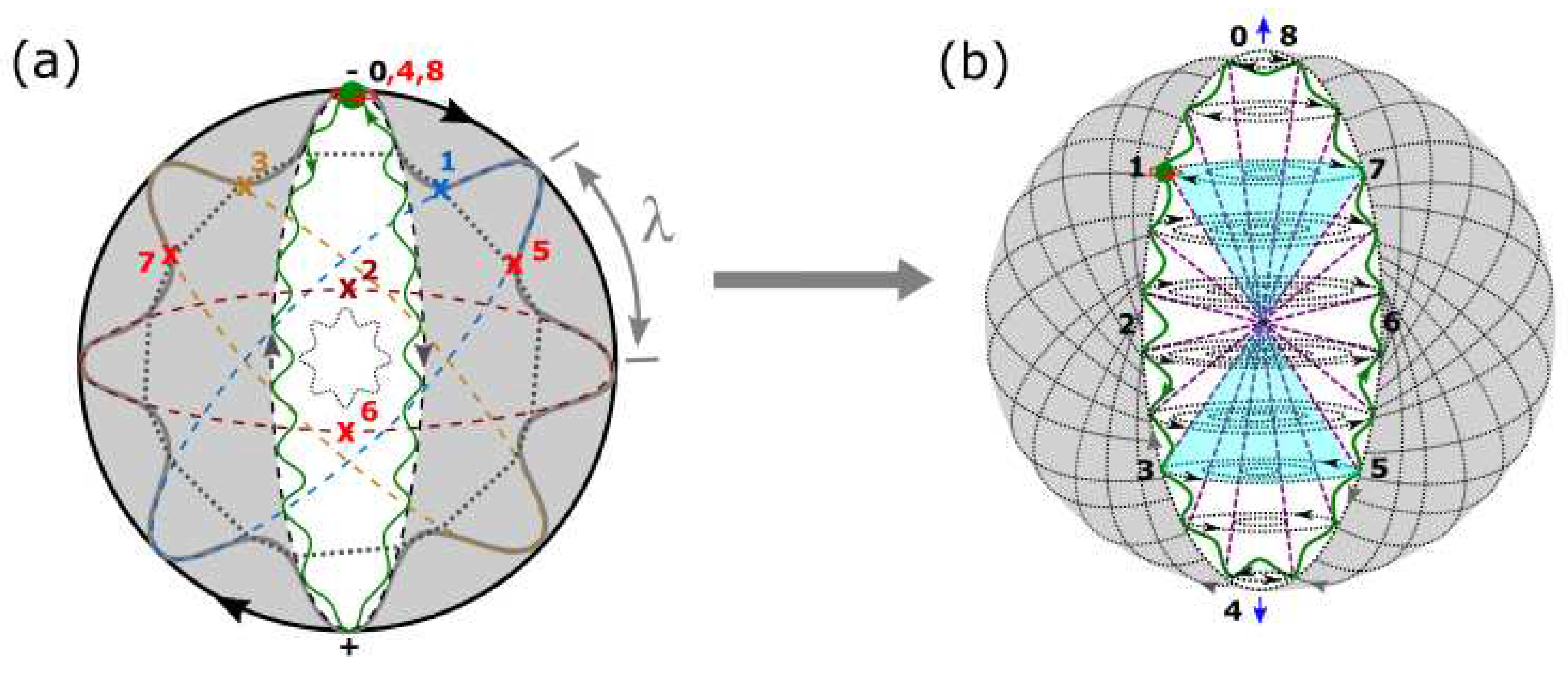
In Figure 1a, an alternative perspective on how the electron of the hydrogen of a Bohr model can be converted to a Dirac fermion of four-component spinor in non-abelian Euclidean space-time is offered. Its spin ±1/2 in superposition states of Minkowski space-time is demonstrated in Figure 1b. Based on these illustrations, a number of postulates are drawn from the first principle of space-time.
- 1)
- The electron’s orbit of time reversal is defined by h of sinusoidal wavy form and is linked to Bohr orbits (BOs) into n-dimensions of energy levels. Its transformation to an elliptic form is embedded within a MP field of clockwise precession and this insinuates spherical inertia frame with unitarity, λ sustained. Excitation from external light interaction assumes, , whereas the probability of locating the electron is defined by De Broglie relationship, λ = h/p. From Euclidean space-time, the cyclic BO (e.g., positions 1 and 5) in Figure 1a is transformed to angular momentum in Minkowski space-time (Figure 1b). At 360° rotation from positions 0 to 3, maximum twists from the torque of the BOs provide a complex spinor field. Thus, the electron with spin up flips to spin down at position 4 to generate a positron. The unfolding process for another 360° rotation from positions 5 to 8 restores the electron to its original state. This allows the electron to undergo 720° rotation within a classical spherical rotation of 360° at lightspeed analogous to the Dirac belt trick. Such a scenario offers both local realism and entanglement of electron-positron pairing in violation of lightspeed. In multielectron atoms, multiple MP fields are assumed for the electrons distribution.Figure 1. The MP model [25]. (a) In flat space, a spinning electron’s (green dot) orbit is sinusoidal (green curve) of time reversal. It is embedded within an elliptic MP field (grey area) of a magnetic field, B. Its clockwise precession (black arrows) generates a circular electric field, E of inertia frame defined by λ, and this produces Euclidean 4D space-time. With precession, the electron shifts from positions 0 to 4 at 360° rotation to generate a positron at maximum twists of the BOs. The unfolding process flips the electron to shift in its positions from 5 to 8 for another 360° rotation to assume its original state. In this way, the electron undergoes 720° rotation to assume a dipole moment (±) within a classical spherical rotation of 360° at lightspeed analogous to Dirac belt trick. (b) The BOs defined by the pairings of the numbered positions such as 1,5 and 3,7 translate to angular momentum (purple dotted lines) of spin ±1/2 of a pair of light-cones (navy colored) in Minkowski space-time. This caters for the twisting and unfolding, while the BOs in degeneracy are projected towards singularity at the center.Figure 1. The MP model [25]. (a) In flat space, a spinning electron’s (green dot) orbit is sinusoidal (green curve) of time reversal. It is embedded within an elliptic MP field (grey area) of a magnetic field, B. Its clockwise precession (black arrows) generates a circular electric field, E of inertia frame defined by λ, and this produces Euclidean 4D space-time. With precession, the electron shifts from positions 0 to 4 at 360° rotation to generate a positron at maximum twists of the BOs. The unfolding process flips the electron to shift in its positions from 5 to 8 for another 360° rotation to assume its original state. In this way, the electron undergoes 720° rotation to assume a dipole moment (±) within a classical spherical rotation of 360° at lightspeed analogous to Dirac belt trick. (b) The BOs defined by the pairings of the numbered positions such as 1,5 and 3,7 translate to angular momentum (purple dotted lines) of spin ±1/2 of a pair of light-cones (navy colored) in Minkowski space-time. This caters for the twisting and unfolding, while the BOs in degeneracy are projected towards singularity at the center.
- 2)
- The electron offers chiral symmetry, where its orthogonal projection, at positions, 0 to 3 is reduced to spin, for the pair of light-cones. Its Hermitian is P(0→8) = with equal to time. The MP model of unitarity gauge obeys the “natural units”, ℏ = c = 1 with the electron’s orbit is accorded to Euler’s formula, + 1 = 0 for continual precession (e.g., Figure 2). Inversion of symmetry at the center violates parity to generate polarization states, ±1 as the dipole moment of MP field. The electron’s position, within a sphere (e.g., Figure 3) incorporates the uncertainty principle, ΔE.Δt ≥ ħ/2 or Δx.Δp ≥ ħ/2 of time invariance. In this way, Schrödinger of an electron cloud model is transformed to a Dirac fermion of a complex four-component spinor field.
- 3)
- The Dirac four-component spinor, assumes its own antimatter at positions, 0, 1, 2 and 3 in Hilbert space when combined with positions 4 to 8 (Figure 1b). The enclosed area defined by the electron shift from positions 0 to 3 is of Euclidean space. Where positions 1 and 3 converge at either position 0 or 2 offers geodesic motion of non-Euclidean space on the surface of the sphere and this somewhat resembles the equivalence principle. By reduction measures such as wave function collapse, only two positions and generate the spin, ±1/2 property of a pair of light-cones. The outcome of the spin is determined by Born’s probabilistic interpretation, , for the wave function collapse scenario (e.g., Figure 3), where the past or future paths of the electron from positions 0 to infinity are not accounted for at observations.
3.2. Gravity and multiverse
- 4)
- How gravity becomes applicable within the MP model is demonstrated in Figure 2. The electron path of sinusoidal wave is of time reversal. The overriding clockwise precession of the MP field induces spherical inertia frames at lightspeed. The generated outline forms the event horizon of elasticity comparable to a black hole. Any external observations are assumed at lightspeed to overcome the spinning inertia frame of reference. Einsteinian gravity then becomes applicable, where matter curves space-time and space-time tells matter how to move [26]. The metric tensor in Minkowksi space-time of angular momenta in Hilbert space is assumed towards singularity at the center (Figure 1b). Any external light interaction with the electron-positron pair at 720° rotation or 360° spherical rotation can somehow translate to gravitational wave types by conservation of angular momenta with the nucleus confined to a black hole scenario (Figure 2). Spherical polarization from a complementary pair of photons over large distance would generate entanglement. Each clockwise precession stage is defined by Ω of a von Neumann entropy state. The microcanonical ensemble for the entropy, S = k In Ω offers exponential rise with continuous precession and this is approximated to the k value, where the space-time metric tensor along the BOs are also included.
- 5)
- In a multiverse of the models at a hierarchy of energy scales, the procession ensues in the following manner, nucleus => atom => planet => star => galaxy. Though there is clear distinction to matter between the scales such as life on Earth and gluons at the nucleus, it is possible that the space-time structural frame offered by the MP model is about the same. So the relationship of the electron to an atom is comparable to satellite to planet, planet to star and possibly star to galaxy. In this way, electromagnetic field permeates space, whereas observation of the MP model’s structural frame appears to be an emergent property of matter from external light interactions.
- 6)
- At the solar scale, only a segment of the spherical curvature of the model is observed by redshift such as the rotation of Earth during lunar eclipse. For Mercury, its unusual perihelion precession deviates about 43 seconds of arc per century from Newtonian theory and this is well accounted by general relativity [27]. However, the explicit solution is more complex and restricted to a planet, while relativity does not explain how the effect of space-time curvature on the inertia frame by precession reconciles with singularity. If, however, the MP model is considered, each planet’s sinusoidal orbit of time reversal against overall clockwise precession is attained at a n-dimension of the sun at the solar scale [25]. Precession is applicable to all the planets, where distinction can be made wherever possible unlike the microscale. For distal objects, considerable redshifts are expected for light waves propagating in space. Such a possibility could explain rotation of galaxies, gravitational lensing, black hole and so forth when these are not ably catered for by general relativity. So with gravity confined to matter in space, the electromagnetic field permeates a multiverse of the models at a hierarchy of scales.
The above postulates with respect to the transformation of the electron to Dirac fermion within the MP model of 4D space-time are pertinent to the tenets of physics. The model is shown to link conventional interpretation of quantum mechanics to gravity, which is generally difficult to attain the conventional way. Based on these interpretations, both relativistic and non-relativistic aspects of the atomic state are explored from an alternative perspective in accordance with existing knowledge in physics.
4. Theoretical outcomes and interpretations
The dynamics of the MP model of 4D space-time physically incorporate well the transformation of the electron to Dirac fermion with both relativistic and non-relativistic features sustained (see Section 3). Some of the possible outcomes are demonstrated in the following order; spinor and helicity, basics of Schrödinger and wave function collapse scenario. Towards the end, the implications to the SM and spin-orbit coupling splitting process are explored.
4.1. Chirality of the MP model
The vector gauge invariance of the Dirac fermion fields, exhibit chiral symmetry by the relationships,
or
The exponential factor, iθ provides both the position, i and angular momenta, θ, for the unitary rotations of right-handedness (R) or positive helicity and left-handedness (L) or negative helicity. Both helicities are projections operators acting on the spinors such as,
and
where is Dirac matrices of eigenstates for the spinor field at fixed momentum. The usual properties of the projection operators are: L + R = 1; RL = LR = 0; L2 = L and R2 = R. Without getting into the intricate details, somehow Equations 4 to 7 are accommodated within the MP model (Figure 1a,b). For example, the electron’s orbit at 360° rotation from positions 0 to 3 within a clockwise precession of the MP field insinuates a positron of positive helicity at position 4 (Figure 3a). Maximum twists from the torque of the BOs provide a complex spinor field equivalent to , where spin up flips over to spin down in anticlockwise direction of time reversal to precession (Figure 3b). The unfolding process at 720° rotation restores the electron of negative helicity with spin up at position 8 or 0. The twisting and unfolding process is attained within a classical rotation of 360° at lightspeed and this compares well with Dirac belt trick. Hence, the isospin of electron allows for transformation of charge conjugation, parity and time reversal simply known as CPT symmetry. Its orbit occupies a hemisphere and this equates to spin 1/2, while its negativity is attributed to clockwise precession (Figure 1a and Figure 3a). Two successive rotations of the electron in violation of lightspeed is identified by and the vector axial current allows for polarization of ±1 of the model depicting chirality. How these descriptions are applicable to matter in a multiverse at a hierarchy of scales (Postulate 5) is beyond the scope of this paper.
4.2. The basis of Schrödinger wave function
The wave-particle duality of the electron is described by the Bohr model of the hydrogen atom and is applicable to Figure 4. By considering the electron to be a charged particle, its orbit of
time reversal due to Einsteinian gravity (Figure 2) is expected to curve the clockwise precession of the MP field to induce spherical inertia frame of reference (e.g., Figure 2). Its evolution with time adheres to the generic non-linear Schrödinger equation,
Equation 8 is of first order in space-time and ℏ describes the sinusoidal form of the orbit (Postulate 1). The Hamiltonian for the electron-positron pair (Equation 3) is demonstrated in Figure 1a,b and Figure 3a. In 3D space, the non-relativistic Schrödinger’s electron field, is defined by the spherical polar coordinates, Ω, Φ, θ with respect to the Cartesian coordinates, x, y, z (Figure 4). The angular component is assigned to the BOs and is demarcated by θ. A diagonal pair of BOs encompasses a pair of light-cones into Minkowski space-time is applicable to Pauli matrices (Figure 1b). The magnetic momentum, Φ is related to the BO and is of a cylindrical boundary within the MP field. The precession of the model then assumes the integrals [29],
where the polar coordinates for the axes are, , and (Figure 4). In high-order Poincaré sphere, the electron vector path of a spinor loop (Figure 1b) is assumed by Berry framework state [30,31,32], of a circuit (C) at polarization with respect to clockwise precession of the MP field. Each precession stage provides additional phase to the dynamics of the model. With radiation given off, Equation 4 is alternatively interpreted as [30],
where S is the surface area with and ρ is the density of the BOs within the MP field defined by Ω (Figure 2). By substituting the vector potential, for the electron path (Figure 2), the resulting Berry phase is given by,
where is a function of , r, and by precession it provides integer order of high-order Poincaré sphere [31], . m is a function of aligned to the BO and is assumed in perpendicular direction to the electron’s position (Figure 4). σ is defined by the twisting and unfolding of degenerate states of BOs to 720° rotation of Dirac belt trick to generate the polarization states, ±1 (Figure 1a). By geometric comparison, this somehow mimics helical cholesteric ordering by left- or right-handedness [31], observed in chiral liquid crystals. The particle’s unique optical state, of is described by,
where the spinor, represents the influx of the magnetic field at the BOs in degeneracy in
Minkowski space-time (Figure 1b). The electron path at 720° rotation (Figure 1a) has two degrees of freedom for the generation of electron ( and the positron . The clockwise precession of the electron, obeys the Euler’s form, (Postulate 2). These explanations relate to the dynamics of the MP model and they can be further explored into depth for both spin photonics and complex Schrödinger equation as a function of time.
4.3. Wave function collapse scenario
The electron of the MP model of a hydrogen atom provides a local gauge group (Figure 5). Its elliptical orbit aligned on a straight path in Minkowki space-time is of circular polarized plane
[32] of a magnetic field, B and is orthogonal to a cyclic electric field, E. The transition at positions 0 to 8 (Figure 1a,b) transforms the electron to a global gauge symmetry at observation. In this way, the electron assumes both local realism and entanglement. Multiple slits are envisioned for the electron path (Figure 3). The translation of its hemisphere to multi-order Feynman diagrams (Figure 4a,b) and this accommodates the orthogonal duality of E and B. The model of a gauge group obeys the “natural units”, ℏ = c =1 (Postulate 2), where other physical constants like the fine-structure constant, α, vacuum permittivity, , reduced Planck
Figure 6.
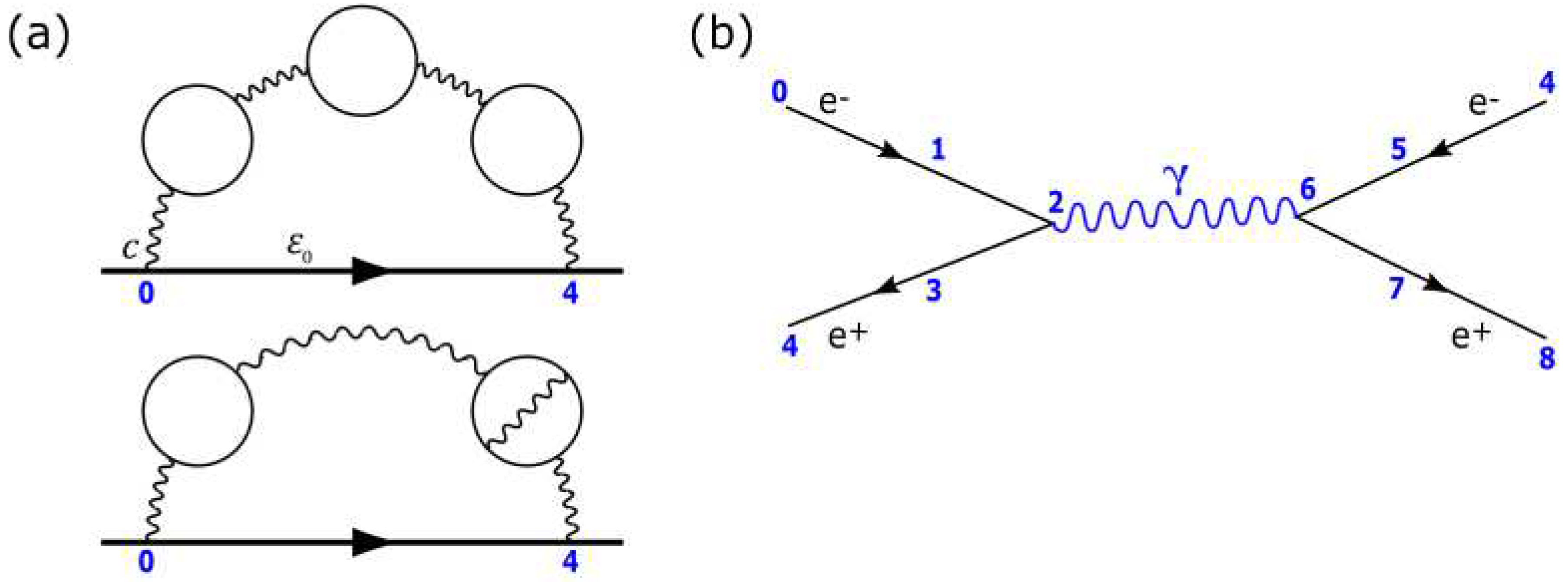
The general consequences of the electron-positron pair. (a) Orthogonal relationship of E and B for eight-order Feynman diagrams of the electron-self interaction within a hemisphere [33] is somewhat comparable to Figure 3 representation in Minkowski space-time. For example, the arrowed horizontal line represents the actual electron path, which acquires electron-positron pair. Wavy lines are virtual photons with the circles assigned to assumed precession stages of the MP field in Hilbert space. The applicability of the physical constants like, and c are demonstrated, while ℏ and are provided in Figure 3. (b) The processes described are transferrable to a generic Feynman diagram inclusive of time reversal.
Figure 6.
The general consequences of the electron-positron pair. (a) Orthogonal relationship of E and B for eight-order Feynman diagrams of the electron-self interaction within a hemisphere [33] is somewhat comparable to Figure 3 representation in Minkowski space-time. For example, the arrowed horizontal line represents the actual electron path, which acquires electron-positron pair. Wavy lines are virtual photons with the circles assigned to assumed precession stages of the MP field in Hilbert space. The applicability of the physical constants like, and c are demonstrated, while ℏ and are provided in Figure 3. (b) The processes described are transferrable to a generic Feynman diagram inclusive of time reversal.
constant, ℏ and lightspeed, c become applicable. The electron charge, and the reciprocal of the mystical dimensionless value [34,35], as 1/137 can be accounted for by the model. Light ray, of circular polarized plane (e.g., Equation 5) provides the four-component spinor field, of Dirac fermion () (e.g., Figure 3). is time in asymmetry at position 0 of Minkowski space-time and the rest are exponentials of Dirac matrices in repetitive process for the electron in orbit. Its reduction to relates to the antisymmetric product of one-particle solutions [36] in the general form,
is the probability operator for the Hermitian of the spin 1/2 property. is provided in Equation 10 and it represents both u- and v-type particles respectively in either inward or outward direction (e.g., Figure 3a and Figure 4). The outcome of is deterministic for the wave function collapse (Equation 13b). These interpretations are somehow consistent with experiments violating Bell’s inequality tests [37,38] supposing that multielectron are applicable to multiple MP fields for many-body system (Postulate 1) and their interactions with photons pairs can somehow correlate at a distance.
5. Implications to the basics of Standard Model
5.1. Electromagnetism and electron spin-orbit splitting
Transformation of U(1) gauge symmetry of infinite number of degrees of freedom for the electromagnetic field is of time invariance accommodates both radial and angular wave distributions (Figure 7a–c(i),(ii). The generation of E from 180° classical rotation orthogonal to B at positions 0 to 4 or 4 to 8 of reverse spin in repetitive mode at the event
horizon of the gauge field somewhat mimes a black hole radiation (Postulates 2 and 4). The variation in the curvature of the event horizon of inertia frame is enlarged in a multiverse at a hierarchy of scales (Postulate 6) so the electromagnetic field of linear time can contract or expand in accordance with classical Maxwell’s equation of the general form,
where is the divergence of the dipole moment of the MP field during precession and is the spin momentum of the electron. The shift in the electron’s position about the BO of angular momentum (Postulate 1) is offered by Faraday’s relationship,
and
The density, ρ of the vacuum state within the model is constrained to spherical configurations of precession, Ω (Figure 4). Ω x Ω* is Hermitian of discrete space-time defined by ℏ (Equation 6).
5.2. Nuclear spin and the Standard Model lagrangian
The spin quantum number, Ι for the nucleus is either an integer or a half-integer. For the hydrogen atom, its nuclear spin 1/2 in respond to the applied external magnetic field is shown in Figure 8 with respect to Figure 7c(i),(ii). The magnitude of its angular momentum is quantized,
with the component of the angular moment, . The orientations of the spin and hence, its magnetic moment is 2Ι + 1 relative to an axis, where the hydrogen has two orientations. These interpretations are applicable to the electron spin with further details inclusive of lamb shift offered in Appendix A. In a similar manner, spin-orbit coupling triplet state of Zeeman effect can be explored within the confinement of the proposed model. The explanations briefly demonstrate the concept of the multiverse of the models at a hierarchy of scale, from the nucleus to beyond the solar system (Postulate 5). On this basis, it is plausible to apply the model to the SM. The in depth mathematical framework of the SM is quite complex with its compact form shown in Figure 9.
The electromagnetic field strenght tensor, F is related to the transformation of the vector axial current (Figure 3a) to linear time at observation (Figure 7a–c(i),(ii)), while the index, α for Pauli matrices is applicable to angular momenta into Minkowski space-time, 𝜇, 𝜈 (Figure 1b). The electron’s isospin of 720° rotation within a classical rotation of 360° at positions 0 to 8 during precession (Figure 3a) offers the Dirac operator, and is subject to correction imposed by hermitian conjugate (h.c). The matter fields of fermions acquire mass by Yukawa coupling to the Higgs field, Φ during electroweak symmetry breaking. The flavor from mixing of the matter fields is sourced from a pool of three leptons, six quarks, three Cabibbo-Kobayashi-Maskawa angles and a CP-violating phase [42]. These properties in a simplified version are intuitively applicable to the electron helical states (Figure 3a,b), where quantization of the sinusoidal wave of unidirecitonal is linked to the BOs defined by Φ and these offer both quadratic and quartic couplings by precession comparable to the Higgs field (Figure 4). Such assumption implies unitarity for the conservation of angular momenta at interactions, where removal of the electron generates a particle-hole symmetry for the vacuum expectation value like the Higgs boson. The continuity of particle-hole (electron) in orbit at high energy would then mimic Nambu-Goldstone bosons [43] as massive version of the photons. In this way, the MP model is applicable to the gauge symmetry, of the SM. The broken symmetries of the electroweak force is given by both abelian hypercharge, Y of the electromagnetic field and non-abelian left-handed, L fermions of a complex 2-vector of chiral flavor symmetry (e.g., Figure 3a). Only the color, C change of charges for the strong nuclear force of non-abelian remains unbroken.
By the explanations offered above, it is plausible to speculate that the electroweak nuclear decay like beta decay, , reinforces the models for both the quark and electron in a multiverse at a hierarchy of scales (Postulate 5). If three generations of both the leptons and quarks are massive versions of the electron and the quark in an onion-like structure of MP models, then W± and Z° bosons mediate their interactions comparable to the photons (e.g., Figure 3a and Figure 7a,b). In this case, the transition between the models in the atom
can somehow relate to either neutrinos at 720° rotation or antineutrinos for 360° rotation in Hilbert space. A possible quark model strictly related to the precession stages of the electron (Figure 3a) is shown in Figure 10. The discussions on how it is applicable to mesons and baryons are briefly summarized on the Wikipedia [44], beginning with the quark field of the types,
and
Equations 16a and b are relatable to Equations 4 and 5 in a multiverse of the models. By substituting and with respect to Figure 10, the baryogensis lagrangian of the strong force then becomes,
where D is the Dirac operator for both matter and antimatter. The 2 x 2 Dirac and Pauli matrices of diagonal relationships is assigned to the BOs in Minkowski space-time. The explicit form of Equation 17 by incorporating both the left- and right-handed spinors of u- and v- types particles in Hilbert space (Figure 5) is of the form,
The reduction of Equation 18 to depict the Dirac process is,
Based on Figure 10, a plethora of particle types can be expected during proton-proton collisions, where the three generations of quarks and leptons are probably massive versions of the electron and quark in an onion-like structure of the model towards singularity.
6. Conclusion
The dynamics of the MP model of 4D space-time considered in this study for the hydrogen atom is somehow able to transform the electron to Dirac fermion of a complex four-component spinor field. Gravity is considered localized in a multiverse of the models at a hierarchy of scales, while electromagnetic field permeate space. Such interpretations though speculative to some extent, the model allows for exceptionally oversimplified intuitions to very complex themes covered by both relativistic and non-relativistic QFTs from the atom to the universe at large. As Erwin Schrödinger, one of the founders of modern physics ably puts it this way [45], “The task is not so much to see what no-one has yet seen, but to think what nobody has yet thought, about that which everybody sees.” These presentations to an extent adapts such a concept from an alternative perspective and this is also comparable to the quest of unifying both quantum mechanics and general relativity. That is trying to integrate what we already know into a proper holistic standpoint before venturing into the unknowns to probe physics beyond the SM and the more complex reality of the physical world.
Competing financial interests
The author declares no competing financial interests.
Appendix A: Electron spin-orbit coupling splitting
The electron spin-orbit coupling splitting is vigorously pursued within the study of quantum electrodynamics (QED). Its pinnacle of success is attributed to the description of the lamb shift when compared to the Dirac field theory (Figure A1b). The lamb shift refines the value of the fine-structure constant, α to about less than 1 part in a billion [46] and it quantifies the gap between the fine structure of the hydrogen spectral lines. It offers a measure of the strength of the electron and its interaction with the electromagnetic field by the relationship [34,35],
In high-energy physics for protons-protons collisions at near lightspeed, a nondimensional system is used with the boundary, = c = ℏ = 1, so Equation 20 is reduced to the form,
The α then provides powers to the perturbative expansion of the anomalous dipole moment of the electron with respect to its g-factor in the form,
The historical ambiguity towards establishing a firm path of calculating the g-factor still remains today, while there is a level of general consensus to about 10 decimal points [47]. But how such information gets translated to the physical world remains ambiguous, while the reciprocal of α for the value of 137 has often left physicists quite mystified of how our universe is fine-tuned.
In this study, it is not one of its purpose to quantify g-factor to a higher level of accuracy but to demonstrate how free parameters like , , ℏ, and so forth can be intuitively related to proposed model as discussed so far. Likewise, diagonal coupling of rotating BOs and would produce intrinsic properties of or the spinor in units of ℏ (Figure A1a) into Minkowski space-time (Figure 1b). The transition from the Bohr model to hydrogen spectral lines and their fine structures defined by the lamb shift (Figure A1b) are somewhat comparable to the degenerate states of BOs. Thus, at zero-point energy at position 0, energy absorption activates the BOs from n = 1 to n = 2 for the spin-orbit coupling of 2P orbital (e.g., Figure 7c(i),(ii)). The reduction of the Dirac fermion of four-component spinor field to spin ±1/2 states for the pair of light-cones is of time invariant to the helical property of the model (Figure 3a).
At position 1 of Minkowski space-time (e.g., Figure 1b), the total angular momentum, , provides the values, and for p orbital at n = 2, l = 1 with respect to BOs in degeneracy. Similarly, the Clebsch−Gordon series for the total orbital angular moment, and total spin, are applicable to the BOs into n-dimensions. For example, the magnitude [29], is assumed for triangulated geometry at positions 0, 2 and 3. The shift in position is dictated by Einsteinian gravity with respect to the arrow of time of a clock face (e.g., Figure 2). These relationships portray the dynamics of the MP model.
Figure A1.
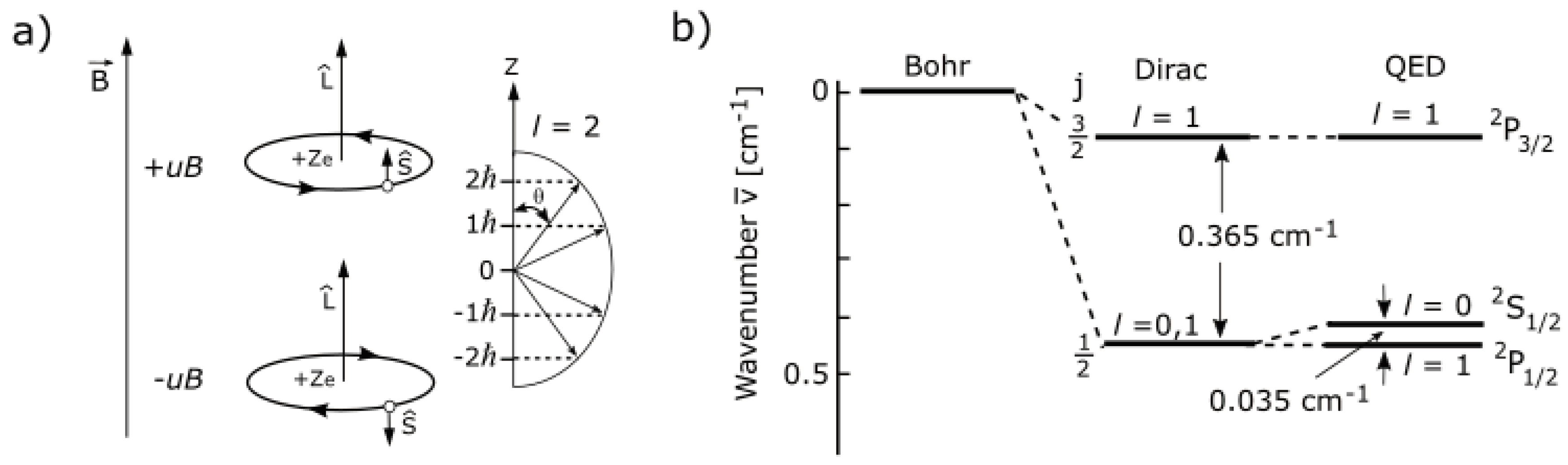
Spin-orbit coupling splitting [29,48]. (a) In the presence of a weak external magnetic field, , its dipole moment, uB of classical Bohr magneton exerts corresponding response from the electron’s dipole moment. The combined dipole is, , with equal to and (e.g., Figure 1b). The electron’s orbit in Hilbert space is quantized, ℏ (e.g., Figure 3) and is aligned perpendicularly to its magnetic momentum, m at the center. (b) When the electron and the MP field dipole moments, i.e., and respectively are aligned to , is produced at high energy such as for a positron (Figure 5c(i)). In the anticoupling process with in the opposite direction, for the electron is assumed at a slightly lower energy than for the lamb shift. This is attributed to the degenerate states of BOs. The pursuits of spin-orbit coupling splitting become more complex from the Bohr model towards QED.
Figure A1.
Spin-orbit coupling splitting [29,48]. (a) In the presence of a weak external magnetic field, , its dipole moment, uB of classical Bohr magneton exerts corresponding response from the electron’s dipole moment. The combined dipole is, , with equal to and (e.g., Figure 1b). The electron’s orbit in Hilbert space is quantized, ℏ (e.g., Figure 3) and is aligned perpendicularly to its magnetic momentum, m at the center. (b) When the electron and the MP field dipole moments, i.e., and respectively are aligned to , is produced at high energy such as for a positron (Figure 5c(i)). In the anticoupling process with in the opposite direction, for the electron is assumed at a slightly lower energy than for the lamb shift. This is attributed to the degenerate states of BOs. The pursuits of spin-orbit coupling splitting become more complex from the Bohr model towards QED.
Appendix B: Application of Dirac field theory
In Figure A1a,b, the applicability of Dirac field theory and hence, QED to the MP model is demonstrated. How this could actually accommodate the Dirac field theory is explored next. The theory is very well developed and is more complex with numerous literatures available. In here, certain aspects of the field theory [1,2,10,11] are copied here in order to demonstrate their relevance to the transformation of the electron to Dirac fermion (e.g., Figure 3a,b) as shown in this study. Thus, the discussions that follows are generally referenced to both the figures and postulates of the conceptualized model as offered in the main text.
Dirac field. Lorentz transformation of the electron to the fermion field of spin ±1/2 is applicable to the MP model. These are denoted ψ(x) in 3D space and ψ(x,t) in both Euclidean and Minkowski space-times (Figure 1a,b). The Dirac equation for the fermion field is given by,
where are the gamma matrices related to the shifts in the electron position of time reversal due to gravity. The exponentials of the matrices, are assigned to positions, 0, 1, 2 and 3 of BOs (Postulate 2). relates to arrow of time in asymmetry at position, 0 for a monopole field and variables to Dirac matrices in 3D space. These are all incorporated into the famous Dirac equation,
where the lightspeed, c acts on the coefficients A, B and C and transforms them to and . Alternatively, the exponentials of are denoted i, where is off-diagonal Pauli matrices at and with respect to the pair of light-cones in Minkowski space-time (Figure 1b). This is defined by,
and zero exponential, to,
is applicable to intersections of the BOs along the electron path for the anticommutation relationship, of the Lie algebra group (Figure 1a). The matrices, 0 and 1 of Equation 25b is relatable polarization of the model.
Weyl spinor. The Weyl spinor of the pair of light-cones is applicable to the precessing MP field at the four positions, 0 to 3 of BOs (Figure 1a). This is represented as,
and it correspond to spin up fermion, a spin down fermion, a spin up antifermion and a spin down antifermion in Hilbert space at 720° rotation comparable to Majorana fermions (e.g., Figure 1a). By relativistic transformation, observation is reduced to a bispinor,
where are the Weyl spinors of chiral form and are irreducible within the model (Figure 3a). Parity operation x → x’ = (t, ‒ x) for qubit 1 and −1 along the vertical axis exchanges the left- and right-handed Weyl spinor (e.g., Figure 3a,b) in the process,
The Weyl spinors are converted to Dirac bispinor, diagonally at positions 1 and 3 of BOs (Figure 1b). Normalization of the two-component spinor, = 1 ensues by the orthogonal relationship, and for the full rotation of the sphere (e.g., Figure 1a).
Lorentz transformation. The Hermitian, for the Dirac fermion transiting at positions, 0, 1, 2 and 3 of BOs is not Lorentz invariant for measurement into 1D space. These states are in superposition but are deterministic at observations (Postulate 3). Thus, by Lorentz transformation, Weyl spinor of a light-cone depicts the relationship,
Equation 29 relates to Minkowski space-time for the spinor provided by the BOs of inertia reference frame (Figure 1b). The corresponding Lorentz scalar of the BOs is,
and is referenced to time axis of the MP field of a dipole moment in asymmetry. By identical calculation to Equation 29, the Weyl spinor becomes,
for the complete classical rotation of the sphere at 360°. Based on the model, it is difficult to distinguish both Weyl spinor and Majorana fermion from the Dirac spinor by relativistic transformation at constant lightspeed.
Quantized Hamiltonian. The 4-vector spinors of Dirac field, (x) offers a level of complexity to observations such as for the Dirac belt trick. Only two ansatzes to Equation 23 are adapted as follow,
These are Hermitian plane wave solutions and they form the basis for Fourier components in 3D space (e.g., Figure 7c(i),(ii)). Decomposition by Hamiltonian then assumes the relationships,
The coefficients and are ladder operators, which are applicable to the BOs into n-dimensions along the orbital paths. These are for u-type particles and similar process is accorded to and of v-type particles (e.g., Figure 5). With unitarity sustained, Hilbert space of the model can expand or contract from external light interactions, where both types of particles are incorporated. The terms, and are Dirac spinors for the two spin states, ±1/2 and and as their antiparticles. The conjugate momentum is,
Equation 34 is assumed by the electron in orbit of 3D space against clockwise precession of the MP field of 4D space-time (Figure 4). The generated oscillations of lagrangian mechanics and its Hamiltonian in 3D space is given by,
The quantity in the bracket is the Dirac Hamiltonian of one-particle quantum mechanics as provided in Equation 3. With z-axis aligned to time axis in asymmetry for a monopole field of a hemisphere (Figure 3a), the V-A currents are projected in either x or y directions in 3D space (e.g., Figure 7a and b) by the relationships,
where α and β denote the spinor components of the . The independent of time in 3D space obeys the uncertainty principle with respect to the electron’s position, p and momentum, q, as conjugate operators. Their commutation relationship obeys the relationship,
Equation 37 incorporates both matter and antimatter, where observation is of linear time (Figure 7a–c(i),(ii)). Thus, a positive-frequency is represented by,
In this way, Dirac strings are constrained with the model and its transformation to orthogonal duality of E and B of linear time.
Further undertakings. The above interpretations demonstrate the compatibility of the model to incorporate relativistic transformation of the electron to a Dirac fermion. Other related themes that can perhaps be pursued in a similar manner include Fock space and Fermi-Dirac statistics, Bose-Einstein statistics, causality, Feynman propagator, charge conjugation, parity, charge-parity-time symmetry and so forth. In this case, the boundary posed by the model could justify the removal of infinities to conform to measurements during renormalization process by assuming unitarity (Postulate 2).
References
- Peskin, M. E. & Schroeder, D. V. An introduction to quantum field theory. Addison-Wesley, Massachusetts, USA (1995).
- Alvarez-Gaumé, L. & Vazquez-Mozo, M. A. Introductory lectures on quantum field theory. arXiv preprint hep-th/0510040 (2005).
- Pawłowski, M. et al. Information causality as a physical principle. Nature 461(7267), 1101-1104 (2009). [CrossRef]
- Henson, J. Comparing causality principles. Stud. Hist. Philos M. P, 36(3), 519-543 (2005). [CrossRef]
- Li, Z. Y. Elementary analysis of interferometers for wave—particle duality test and the prospect of going beyond the complementarity principle. Chin. Phys. B 23(11), 110309 (2014). [CrossRef]
- Rabinowitz, M. Examination of wave-particle duality via two-slit interference. Mod. Phys. Lett. B 9(13), 763-789 (1995). [CrossRef]
- Nelson, E. Derivation of the Schrödinger equation from Newtonian mechanics. Phys. Rev. 150(4), 1079 (1966). [CrossRef]
- Rovelli, C. Space is blue and birds fly through it. Philos. Trans. Royal Soc. Proc. Math. Phys. Eng. 376(2123), 20170312 (2018). [CrossRef]
- Perkins, D. H. Proton decay experiments. Ann. Rev. Nucl. Part. Sci. 34(1), 1-50 (1984). [CrossRef]
- Sun, H. Solutions of nonrelativistic Schrödinger equation from relativistic Klein–Gordon equation. Phys. Lett. A 374(2), 116-122 (2009). [CrossRef]
- Oshima, S., Kanemaki, S. & Fujita, T. Problems of Real Scalar Klein-Gordon Field. arXiv preprint hep-th/0512156 (2005).
- Bass, S. D., De Roeck, A. & Kado, M. The Higgs boson implications and prospects for future discoveries. Nat. Rev. Phys. 3(9), 608-624 (2021). [CrossRef]
- Weiss, L. S. et al. Controlled creation of a singular spinor vortex by circumventing the Dirac belt trick. Nat. Commun. 10(1), 1-8 (2019). [CrossRef]
- Silagadze, Z. K. Mirror objects in the solar system?. arXiv preprint astro-ph/0110161 (2001).
- Almasi, A. et al. New limits on anomalous spin-spin interactions. Phys. Rev. Lett. 125(20), 201802 (2020). [CrossRef]
- Yang, C. N. & Mills, R. Conservation of isotopic spin and isotopic gauge invariance. Phys. Rev. 96, 191 (1954). [CrossRef]
- Gross, D. J. Nobel lecture: The discovery of asymptotic freedom and the emergence of QCD. Rev. Mod. Phys. 77(3), 837 (2005). [CrossRef]
- Gell-Mann, M. & Low, F. E. Quantum electrodynamics at small distances. Phys. Rev. 95(5), 1300 (1954). [CrossRef]
- Arkani-Hamed, N. et al. Solving the hierarchy problem with exponentially large dimensions. Phys. Rev. D 62(10), 105002 (2000). [CrossRef]
- Higgs, P. Spontaneous symmetry breakdown without massless bosons. Phys. Rev. 145, 1156 (1966). [CrossRef]
- Craig, N. Naturalness hits a snag with Higgs. Physics 13, 174 (2020). [CrossRef]
- Douglas, M. R. Report on the status of the yang-mills millennium prize problem. Preprint. http://www. claymath. org/millennium/Yang-Mills Theory/ym2.Pdf (2004).
- Howard, D. Who invented the “Copenhagen Interpretation”? A study in mythology. Philos. Sci. 71(5), 669-682 (2004).
- Wineland, D. J. Nobel lecture: Superposition, entanglement, and raising Schrödinger’s cat. Rev. Mod. Phys. 85(3), 1103 (2013).
- Yuguru, S. P. Unconventional reconciliation path for quantum mechanics and general relativity. IET Quant. Comm. 3(2), 99–111 (2022). [CrossRef]
- Misner, C. W., Thorne, K. S & Zurek, W. H. John Wheeler, relativity, and quantum information. Phys. Today 62(4), 40-46 (2009).
- Bootello, J. Angular Precession of Elliptic Orbits. Mercury. Int. J. Astron. Astrophys. 2(4), 249-255 (2012). [CrossRef]
- https://en.wikipedia.org/wiki/Spinor Retrieved 15 December 2022.
- Atkins, P. & de Paula, J. Physical Chemistry. 9th Edition. Oxford University Press, New York (2010).
- Yi, X. et al. Hybrid-order Poincaré sphere. Phys. Rev. A 91(2), 023801 (2015).
- Milione, G. et al. Higher-order Poincaré sphere, Stokes parameters, and the angular momentum of light. Phys. Rev. Lett. 107(5), 053601 (2011).
- Rafayelyan, M. & Brasselet, E. Spin-to-orbital angular momentum mapping of polychromatic light. Phys. Rev. Lett. 120(21), 213903 (2018). [CrossRef]
- Examples of 8-order Feynman diagrams for electron propagation, Wikimedia Commons https://en.wikipedia.org/wiki/Image:EighthOrderMagMoment.svg Retrieved 24 November 2022.
- Kragh, H. Magic number: A partial history of the fine-structure constant. Arch. Hist. Exact Sci. 57(5), 395-431 (2003). [CrossRef]
- Sherbon, M. A. Fundamental nature of the fine-structure constant. Int. J. Phys. Res. 2(1), 1-9 (2014). [CrossRef]
- Szabo, A. & Ostlund, N. S. Modern quantum chemistry: introduction to advanced electronic structure theory. Courier Corporation, Massachusetts, USA (1996).
- Aspect, A., Grangier, P. & Roger, G. Experimental realization of Einstein-Podolsky-Rosen-Bohm Gedankenexperiment: a new violation of Bell's inequalities. Phys. Rev. Lett. 49(2), 91 (1982).
- Pan, J. W. et al. Experimental entanglement swapping: entangling photons that never interacted. Phys. Rev. Lett. 80(18), 3891 (1998). [CrossRef]
- Weil, J. A. & Bolton, J. R. Electron paramagnetic resonance: elementary theory and practical applications. John Wiley & Sons (2007). [CrossRef]
- Lindon, J. C., Tranter, G. E. & Koppenaal, D. Encyclopedia of spectroscopy and spectrometry. Academic Press (2016).
- Woithe, J., Wiener, G. J., & Van der Veken, F. F. Let’s have a coffee with the standard model of particle physics!. Phys. Educ. 52(3), 034001 (2017). [CrossRef]
- Ellis, J. Outstanding questions: physics beyond the Standard Model. Philos. Trans. A Math. Phys. Eng. Sci. 370 (1961), 818-830 (2012). [CrossRef]
- Freese, K., Frieman, J. A. & Olinto, A. V. Natural inflation with pseudo Nambu-Goldstone bosons. Phys. Rev. Lett. 65(26), 3233 (1990). [CrossRef]
- https://en.wikipedia.org/wiki/Chirality_(physics) Retrieved 26 October 2022.
- Moore, W. Schrӧdinger. Life and thought. Cambridge University Press, London, 1989. p. 513.
- Gabrielse, G. et al. New determination of the fine structure constant from the electron g value and QED. Phys. Rev. Lett. 97(3), 030802 (2006).
- Consa, O. Something is wrong in the state of QED. arXiv preprint arXiv:2110.02078 (2021).
- Hanneke, D. et al. Cavity control of a single-electron quantum cyclotron: Measuring the electron magnetic moment. Phys. Rev. A 83(5), 052122 (2011). [CrossRef]
Figure 2.
The applicability of gravity to the MP model. The electron’s orbit of sinusoidal wave (dark green) is of time reversal and is attributed to Einsteinian gravity [25]. External observation of Newtonian gravity or extraction of any other information from the model is restricted to the spherical outline of inertia frame as the event horizon due to the clockwise precession of the MP field (i.e., a black hole scenario). The nucleus is confined, while the elasticity of the model can allow for asymptotic freedom by expansion and contraction with conservation of angular momenta during interactions.
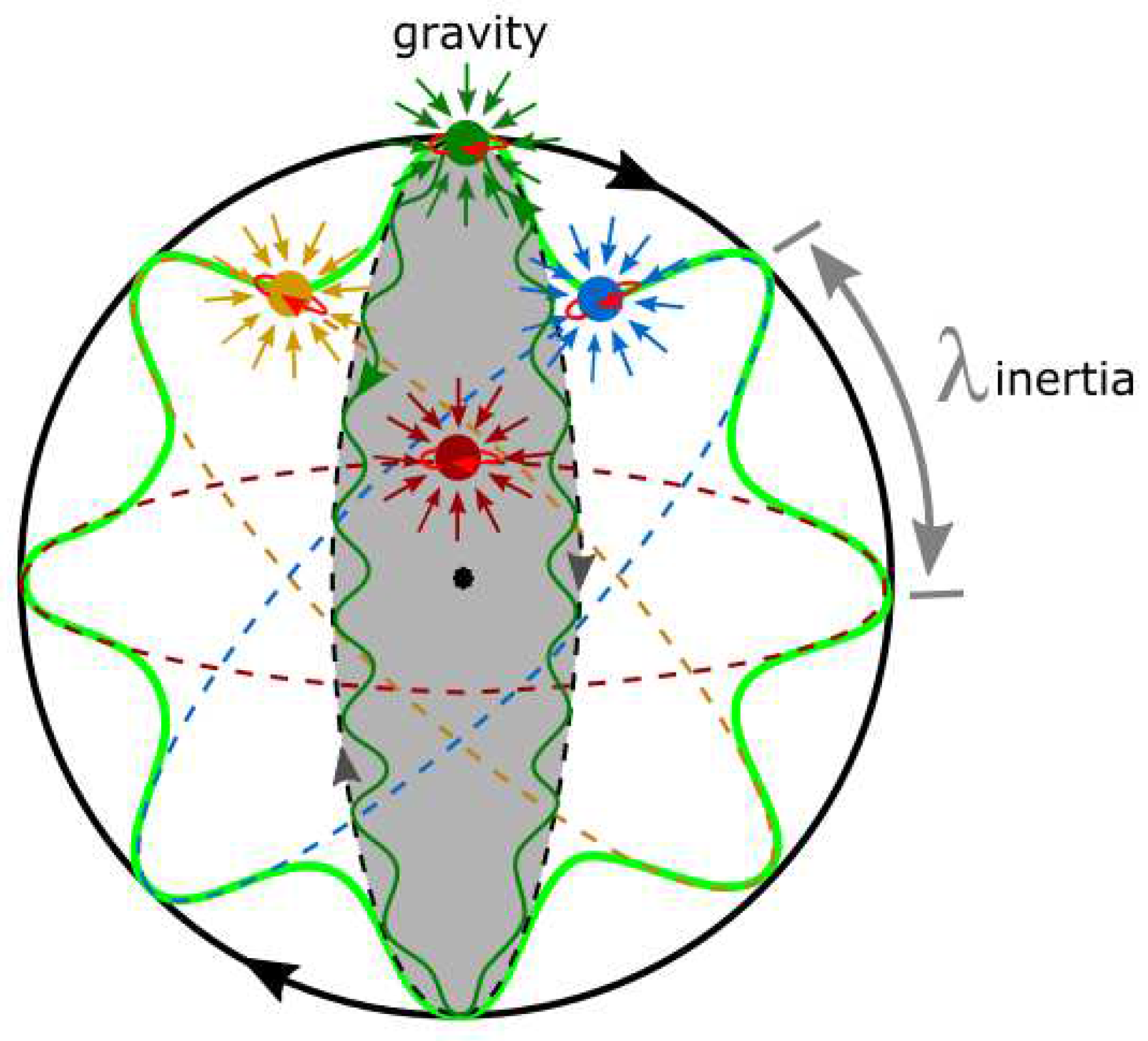
Figure 3.
(a) The electron of negative helicity is assumed for spin up in the same direction as the outward clockwise precession of the MP field. Once maximum twists provided by the torque of the BOs are reached at 360° rotation, the electron’s spin flips downward at position 4. The spin then resumes anticlockwise direction of reversal time to precession, where a positron of positive helicity is generated. The unfolding process towards 720° rotation from shifts in positions 5 to 8 restores the electron to its original state. (b) Both twisting and unfolding processes are attained at a classical rotation of 360° at lightspeed. The electron path of vector transport precesses at Lamour frequency. The polarization of the model produces qubits 0 and ±1 with respect to Figure 1a. Image adapted from ref. [28].
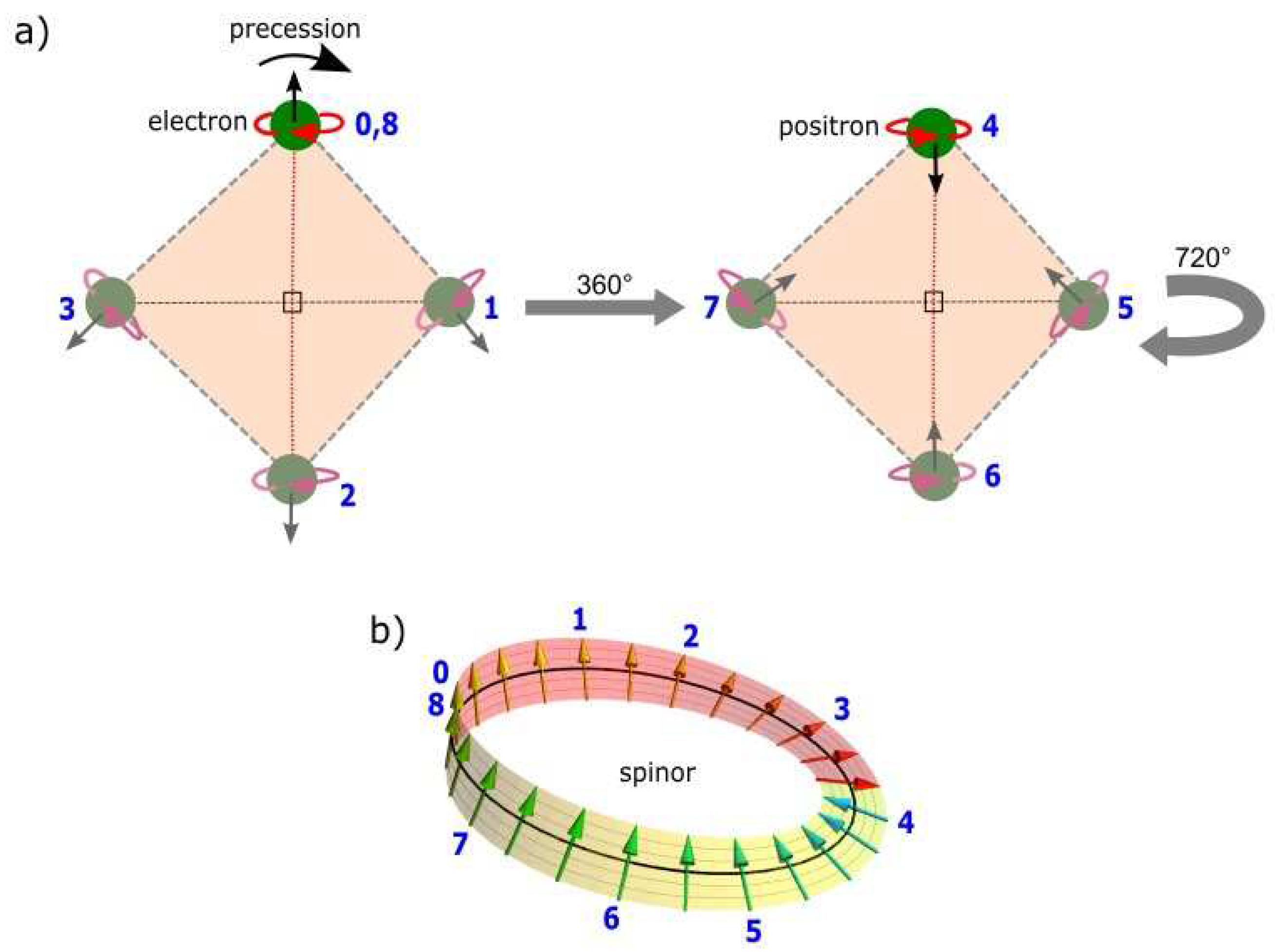
Figure 4.
Harmonic oscillation. The electron of Schrödinger (green wavy curve) is confined to a MP field. Its clockwise precession induces electric charge field of Berry (geometric) phase-like on a high-order Poincaré sphere. The electron as a physical entity (insert image) in Minkowski space-time acquires mass by oscillation comparable to a planetary body in orbit of the sun (see also Figure 1b). The symbols, Ω, Φ, θ relate to the polar coordinates and r is the radial component. Image modified from ref. [29,30].
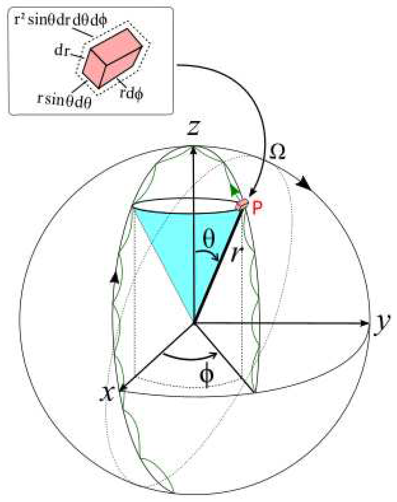
Figure 5.
A wave function collapse scenario. The electron (green circle) in its path of clockwise precession, is defined by wave-particle duality. Its transformation at observation for a double slit experiment identifies with Born’s probabilistic interpretation,, where the wave function collapses to a deterministic value (see also Postulate 3). The electron’s path at positions 0 to 8 generates both u- and v-type particle-like properties in Hilbert space with respect to the center of the sphere (e.g., Figure 1a,b).
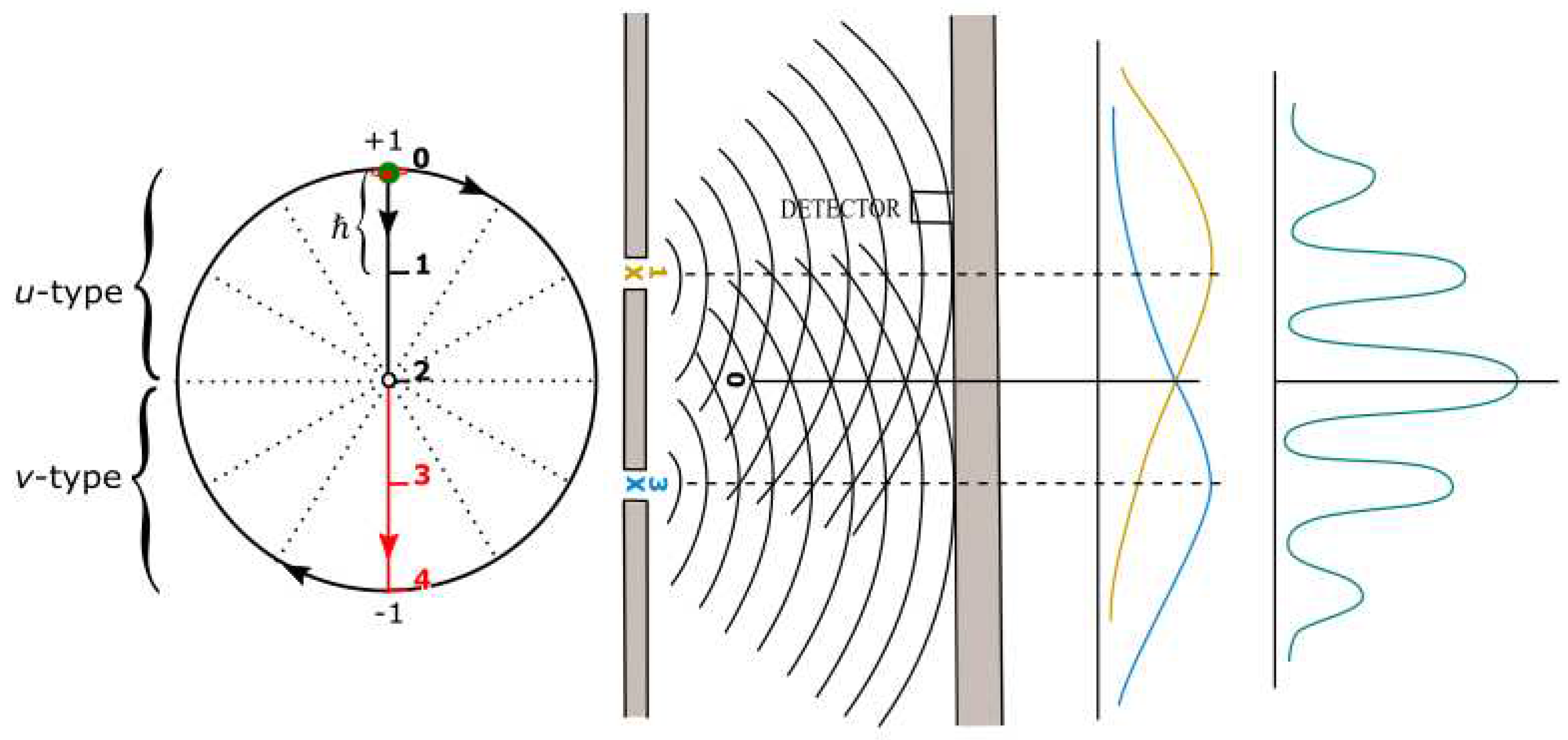
Figure 7.
Generation of the electromagnetic waves from the MP model into space. (a) B is assumed at positions 0 to 4 accompanied by E of a hemisphere (orange colored) at spherical rotation of 180° (e.g., Figure 3). The numbered positions from 9 onwards repeat the process described by positions 0 to 8 of the MP model. (b) Radial distribution of sinusoidal wave both at rest and when disturbed at observation (dotted wavy curve) of elastic property. (c) A. In the presence of a weak external B, the excitation of the model from n = 1 to n = 2 allows for spin-orbit coupling splitting as seen in paramagnetic(spin) resonance [39] and is also comparable to Stern-Gerlach experiment of ±1/2 spin. B. The electron is converted to a positron at position 4 and it is restored at position 8 in violation of lightspeed comparable to the Dirac belt trick (e.g., Figure 1a). The energy difference, ΔE between the spins is proportional to the g-factor (g) and Bohr magneton (β). In repetition, it can apply to Fourier Transform.
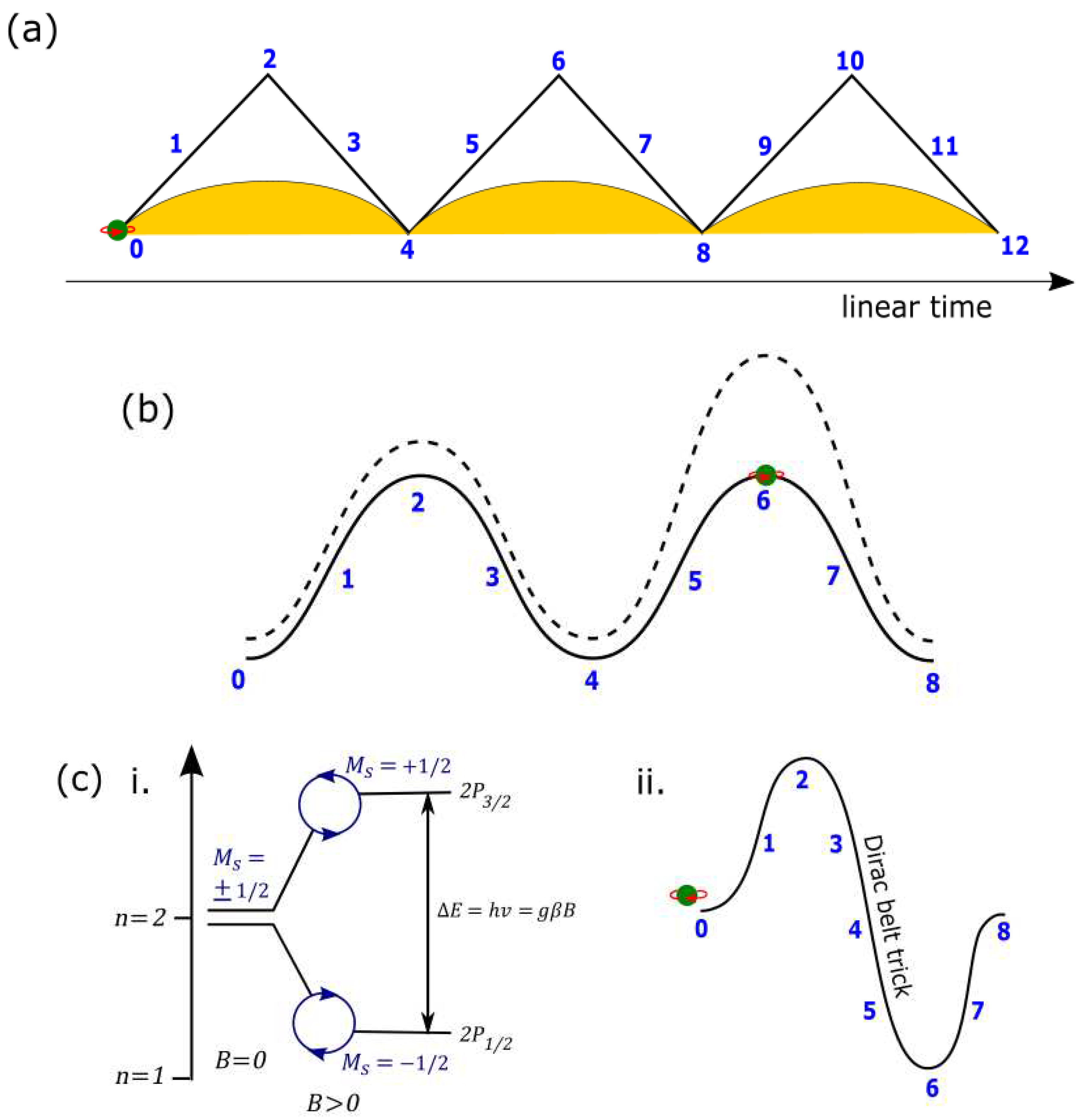
Figure 8.
Spin-orbit coupling splitting [40]. (a) The spin-orbit coupling doublet state incorporates both the electron and the nuclear magnetic spin, (see also Figure 5c(i),(ii)). (b) Hyperfine coupling constant, α of the electron paramagnetic resonance spectra possibly links the MP models between the atom and the nucleus in a possible multiverse scenario (Postulate 4). The selection rule for the nuclear magnetic spin is, compared to the electron, .
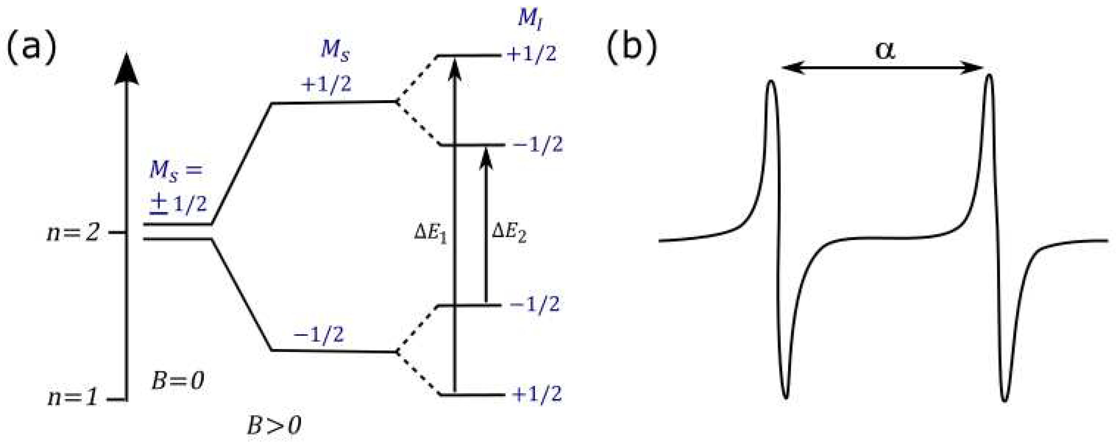
Figure 9.
The compact equation of the Standard Model Lagrangian, with its brief descriptions [41]. Its applicability to the MP model is succinctly described in the text, while more in depth forms of its complexities are available in numerous literatures dealing with relativistic QFTs.
Figure 9.
The compact equation of the Standard Model Lagrangian, with its brief descriptions [41]. Its applicability to the MP model is succinctly described in the text, while more in depth forms of its complexities are available in numerous literatures dealing with relativistic QFTs.
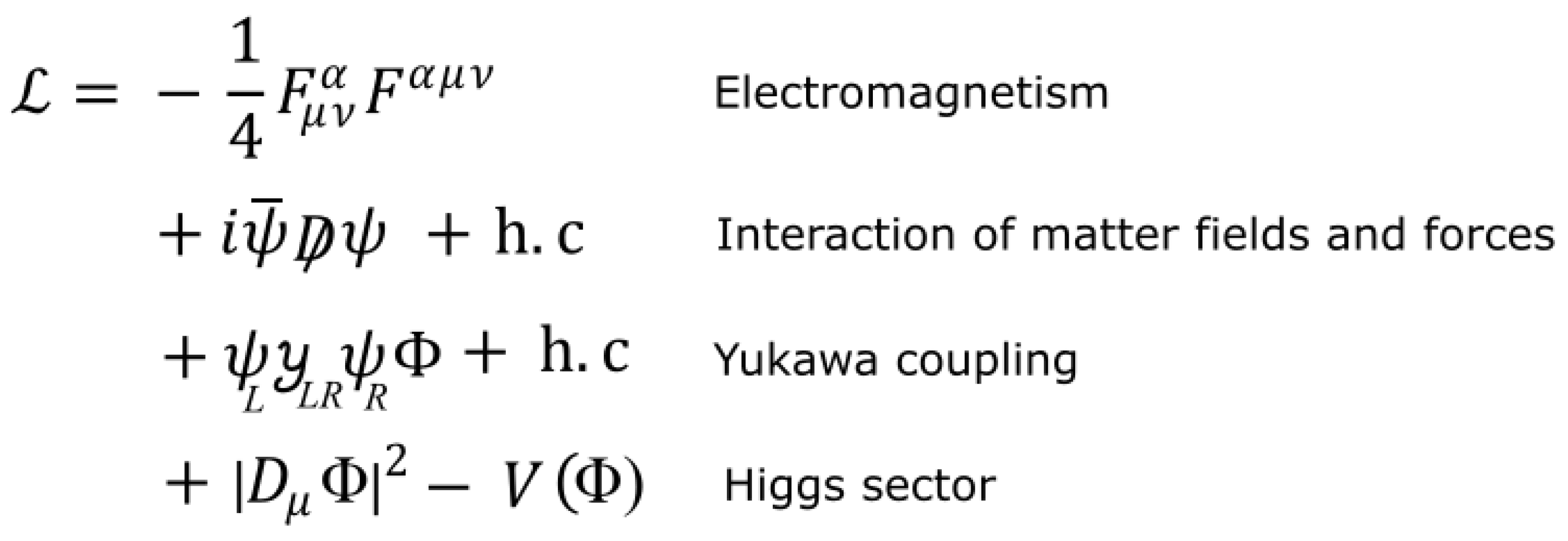
Figure 10.
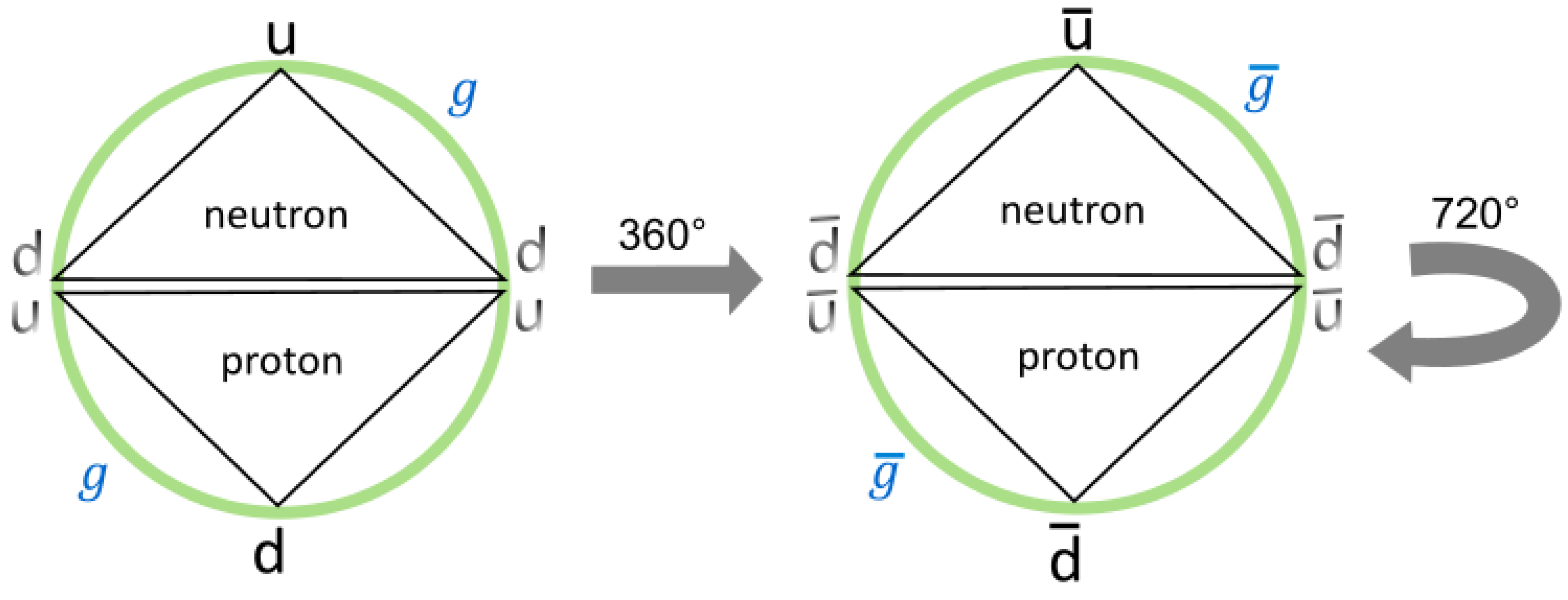
Tetraquark model of and . The faded colored u and d and their antimatter are in a superposition state comparable to of Dirac fermion (Postulate 2). Thus, both up and down quarks are applicable to proton and neutron but the full extent of the color flavor determines the emergence of each particle type.
Figure 10.
Tetraquark model of and . The faded colored u and d and their antimatter are in a superposition state comparable to of Dirac fermion (Postulate 2). Thus, both up and down quarks are applicable to proton and neutron but the full extent of the color flavor determines the emergence of each particle type.
Disclaimer/Publisher’s Note: The statements, opinions and data contained in all publications are solely those of the individual author(s) and contributor(s) and not of MDPI and/or the editor(s). MDPI and/or the editor(s) disclaim responsibility for any injury to people or property resulting from any ideas, methods, instructions or products referred to in the content. |
© 2023 by the authors. Licensee MDPI, Basel, Switzerland. This article is an open access article distributed under the terms and conditions of the Creative Commons Attribution (CC BY) license (http://creativecommons.org/licenses/by/4.0/).
Copyright: This open access article is published under a Creative Commons CC BY 4.0 license, which permit the free download, distribution, and reuse, provided that the author and preprint are cited in any reuse.


