

Submitted:
23 May 2026
Posted:
25 May 2026
You are already at the latest version
Abstract
Physics makes two questionable assumptions: (1) Distant galaxies are accelerating relative to Earth. (2) Entangled objects do not stay together spatially. Why questionable? Acceleration has never been observed in a single galaxy. Observers perceive entangled objects as spatially separated objects, yet 3D space is relative. Here we show: While special and general relativity remain fully valid, additional information is available when we take a 4D Euclidean geometry into account. We calculate relativistic effects (Lorentz factor, gravitational time dilation) from purely geometric considerations and conservation laws. The extra information is helpful for understanding the very distant and the very small. In Euclidean relativity (ER), all objects move through 4D Euclidean space (ES) at the same speed C. Worldlines are parameterized by a monotonically increasing, absolute, external evolution parameter θ. An observer experiences two projections of ES as space and time. The axis of his current 4D motion is his proper time τ. Three orthogonal axes make up his 3D space x1, x2, x3. His physical reality is the “τ-based spacetime” cτ(ϑ), x1(ϑ), x2(ϑ), x3(ϑ), where the observer’s τ is the time coordinate and the parameter θ is converted into parameter time ϑ. ER predicts the Hubble tension and entanglement. Remarkably, ER manages without cosmic inflation, expanding space, dark energy, and non-locality. ER teaches us: (1) Distant galaxies retain their recession speeds. (2) From their perspective, entangled objects have never been spatially separated, yet their proper time flows in opposite 4D directions.
Keywords:
cosmology
; spacetime
; relativity
; dark energy
; quantum mechanics
; non-locality
Clocks measure proper time . There are two ways to use : In special and general relativity (SR/GR) [1,2], is frequently used to parameterize an object’s worldline in spacetime. In Euclidean relativity (ER), is the time coordinate of spacetime. Note that ER does not affect the data describing the universe. It is just a different way of displaying the same data. All we do is interpret the motion of objects in a different geometry. As a matter of fact, we take a purely geometric approach to describing the universe. In particular, we do physics without forces and fields. Thus, our approach does not (!) conflict with SR/GR.
ER predicts (a) cosmic homogeneity without postulating cosmic inflation, (b) galactic motion without postulating expanding space and dark energy, and (c) entanglement without postulating non-locality. In all cases, a 4D vector “flow of proper time” is required. For instance, distant galaxies retain their recession speeds, but their 4D vector deviates greatly from of the Milky Way. Is there a continuous transition between the spacetime in ER and the spacetime in SR/GR? No, the time coordinate and the invariant are fundamentally different in these theories. Does ER make quantitative predictions? Yes, it predicts the 10 percent discrepancy in the published values of the Hubble constant (see Section 5.10).
Important notice to all readers: (1) Do not apply the concepts of SR/GR to ER. The only standards for any scientific theory are its own concepts and empirical facts. (2) Do not reject ER because we do physics without forces and fields. We show that ER reveals new insights into cosmology and the quantum world. (3) Be curious. New coordinates can indeed reveal new insights. In SR/GR, coordinates are labels. They can be adjusted to simplify computations. In ER, coordinates are inherent properties of objects. They cannot be adjusted because they refer to absolute 4D Euclidean space. (4) Be fair. A single paper cannot cover all of physics, yet it can improve our understanding of the very distant and the very small.
1. Introduction
Today’s concepts of space and time were coined by Albert Einstein. In SR, the Minkowski metric describes a flat spacetime. The geometric framework is Minkowski spacetime [3]. The muon lifetime [4] is an often-cited example that supports SR. In GR, the metric tensor and the Einstein tensor describe a curved spacetime. The deflection of starlight [5] and the accuracy of GPS [6] are two examples that support GR. Quantum field theory [7] unifies classical field theory, SR, and quantum mechanics (QM), but not GR.
Newburgh and Phipps [8] pioneer ER. Montanus [9,10] adds a restriction: He considers a preferred reference frame in which a pure time interval is a pure time interval for all observers (see page 351 of [9]). By doing so, he deprives ER of its key feature: full symmetry in all four axes. Montanus claims (see page 17 of [11]): The preferred frame is necessary to avoid “distant collisions” (without physical contact) and a “character paradox” (confusion of photons, particles, and antiparticles). Our formulation of ER does not prefer any frame. There are no distant collisions: Only three axes are experienced as space. There is no character paradox: Photons, particles, and antiparticles are physical concepts. They don’t apply to a mathematical reality. Montanus [10] uses a Euclidean metric to derive gravitational lensing and the precession of Mercury’s perihelion. He even attempts to derive Maxwell’s equations, but he fails because of a wrong sign (see page 92 of [11]).
Almeida [12] analyses geodesics in 4D Euclidean space. Gersten [13] shows that the Lorentz transformation can be interpreted as an SO(4) rotation in mixed space , where is the Lorentz transform of coordinate time . There is also a website about ER: https://euclideanrelativity.com. Previous formulations of ER [8,9,10,11,12,13] merely rearrange the metric of SR to give it a Euclidean appearance. In particular, they still use coordinate time. We take a new approach to make ER work by eliminating coordinate time.
To this day, ER is rejected for various reasons: (a) SR and GR have been confirmed by experiments over and over again. (b) There seem to be geometric paradoxes in ER. (c) ER does not yet reproduce all of GR’s predictions. We show that physics has reached a turning point: (a) No theory is set in stone. (b) Projections avoid paradoxes. (c) SR/GR have been tested for over 100 years. ER is an emerging theory. Anyone who rejects ER because it does not yet reproduce all of GR’s predictions must also reject GR until it reproduces all of ER’s predictions, such as the tension. The same standards apply to all theories!
In Newton’s physics, all objects move through 3D Euclidean space as a function of time. There is no speed limit. In Einstein’s physics, all objects move through a 4D non-Euclidean spacetime as a function of an internal parameter. The speed limit is . In Euclidean relativity, all objects move through 4D Euclidean space as a function of an external parameter. The 4D speed of everything is . Einstein’s physics reduces to Newton’s physics when speeds are low and gravity is weak. ER does not reduce to Einstein’s physics. ER uses a different time coordinate and a different invariant to predict empirical facts (see Section 5).
2. Coordinate Time and Its Shortcomings
In § 1 of SR [1], Einstein considers a reference frame “in which the equations of Newton’s physics hold” (to a first approximation). If an object is at rest in this frame, its position in 3D space is determined using rigid rods and a 3D Euclidean geometry. If we also want to describe an object’s motion, we have to define time. Einstein gives an instruction on how to synchronize clocks at two points P and Q. At a coordinate time , a light signal is sent from P to Q. At , it is reflected at Q. At , it is back at P. The clocks synchronize if
. (1)
In § 3 of SR, Einstein derives the Lorentz transformation. The coordinates of an event in a system K are transformed to the coordinates in K’ by
, , , (2a)
, (2b)
where K’ moves relative to K in at the constant speed and is the Lorentz factor. Eqs. (2a–b) transform the coordinates from K to K’. Covariant equations transform the coordinates from K’ to K. The metric of Minkowski spacetime is
, (3)
where is an infinitesimal change in the invariant , and and all () are infinitesimal distances in coordinate time and 3D space . Minkowski spacetime is a construct because is a man-made concept derived from Eq. (1): is a label that is not inherent in clocks. In GR, retains its function as a label. We identify four shortcomings of : (1) SR/GR work for observers, but SR/GR do not provide diagrams that work for all observers. (2) GR-based cosmology fails to predict time’s arrow and the tension. Other empirical facts can be predicted, but only by postulating highly speculative concepts (cosmic inflation, expanding space, dark energy). (3) -based QM postulates another highly speculative concept (non-locality). (4) GR is probably incompatible with QM.
SR/GR provide observer-specific diagrams (spacetime diagrams): These diagrams do not work for all observers. There are coordinate-free formulations of SR [14] and GR [15,16], but they still lack absolute space and absolute time. In ER, physical realities remain relative, but they are embedded in absolute 4D Euclidean space and parameterized by absolute time. ER provides observer-independent diagrams (diagrams of 4D Euclidean space): These Master Diagrams work for all observers (see Section 3). Physics has paid an enormous price for clinging to coordinate time. ER predicts empirical facts (see Section 5) without postulating highly speculative concepts. ER even predicts time’s arrow and the tension. Thus, the shortcomings of are real. Michelson and Morley [17] refute absolute 3D space (“luminiferous ether”), but not absolute 4D space embedding countless relative 3D spaces.
Neither SR nor GR make false predictions. The shortcomings of have much in common with the shortcomings of geocentrism: GR-based cosmology and -based QM require concepts that are dispensable in ER. In the old days, it was believed that all celestial bodies orbited Earth. Only the astronomers wondered about the retrograde loops of planets and claimed: Earth orbits the sun! Nowadays, it is believed that the universe is expanding. It is our turn to wonder: How could it expand? The standard answer is this: The universe expands by creating new space within itself. Mathematically, the spatial components of the FLRW metric are scaled [18]. Physically, spacetime is an entity. Shouldn’t time also be scaled? Ontologically, “space creating new space” is a very problematic concept.
The analogy between geocentrism and egocentrism in SR/GR is striking: (1) Diagrams of geocentrism are centered in Earth (“geo”). Spacetime diagrams of SR/GR are centered in observers (“ego”). (2) After centering another planet or after a transformation in SR/GR, the diagrams are still geocentric or else egocentric. (3) Retrograde loops make geocentrism work, but are dispensable in heliocentrism. Dark energy and non-locality make cosmology and QM work, but are dispensable in ER. (4) Heliocentrism breaks with geocentrism. ER breaks with egocentrism. (5) Geocentrism was a dogma in the old days. SR/GR are dogmata nowadays. Has physics not learned from history? Is history repeating itself?
3. The Physics of Euclidean Relativity
ER is a new way to describe physical realities. Unlike SR/GR, ER postulates a mathematical background reality. Unlike SR/GR, ER uses a natural time coordinate and an absolute parameter time. Here is how we proceed: To determine an object’s position in an observer’s 3D space, we use the same rigid rods and the same 3D geometry (Euclidean geometry) as in SR. However, we will not use coordinate time as the time coordinate, but the natural, proper time measured by clocks. That is, we do not construct time.
ER postulates: (1) All objects move through 4D Euclidean space (ES) at the same speed . Worldlines are parameterized by a monotonically increasing, absolute, external evolution parameter . (2) An observer experiences two orthogonal projections of ES as space and time. The axis of his current 4D motion is his proper time . Three orthogonal axes make up his 3D space . Orthogonal projections are described in textbooks about geometry [19,20]. (3) The laws of physics take the same form in all physical realities. An observer’s physical reality is the “-based spacetime” . Our first postulate is much stronger than the second SR postulate: is both absolute and universal. Our second postulate is unique to ER. Our third postulate applies to physical realities, but not to ES. The metric of ES is
, (4)
where is an infinitesimal change in the new invariant , and all () are infinitesimal distances in ES. We set the universal speed in ES to . We define an object’s 4D Euclidean vector “ES velocity” with the four speed components . Since an object’s flows in the direction of its 4D motion, it makes sense to define a 4D Euclidean vector “flow of proper time” , which is equal to . According to these definitions, the metric in Eq. (4) is equivalent to our first postulate.
, (5)
. (6)
The quantities , , , are dimensionless. ES is a mathematical reality: There is no time coordinate in ES. We consider two objects “r” (red) and “b” (blue) moving through ES at the speed . Every object is free to label the axes of its reference frame in ES. We can thus assume that “r” (or “b”) labels the axis of its current 4D motion as (or else ) and three orthogonal axes as (or else ). According to our first postulate, “r” (or “b”) always moves in (or else ) at the speed . Because of length contraction at the speed (see Section 4), “r” does not experience the axis as space, but as proper time. It experiences the other three axes as 3D space.
To accomplish the transition from ES to an observer’s physical reality, we add units to , obtaining . We reassemble the axes using the Minkowski signature . We call the result “-based spacetime” (-ST), where the observer’s is the time coordinate and the parameter is converted into parameter time . The observer experiences -ST. The metric of -ST is
, (7)
which differs from Eq. (3) only in that is replaced by , and by . Previous formulations of ER [8,9,10,11,12,13] merely swap and . In -ST, an object’s speed is .
in seconds (s), (8a)
() in light seconds (Ls), (8b)
in light seconds per second, (8c)
() in light seconds per second. (8d)
Mathematically, Eqs. (3) and (7) are identical. Physically, the time coordinate of -ST is not a label that we can adjust, but the proper time of a specific observer. In SR, observers experience a single manifold (Minkowski spacetime), but they do so in observer-specific reference frames. Inertial frames are related to each other by the Lorentz transformation. In ER, observers experience observer-specific projections of a single manifold (ES) and the projections are reassembled to observer-specific spacetimes (-ST). These observer-specific spacetimes are related to each other by a 4D Euclidean rotation (see Section 4).
In SR, the coordinates are , where is a man-made concept and is an internal parameter. In ER, the coordinates of ES are and the coordinates of -ST are , where is a natural concept. and are external parameters. is natural because it is measured by (thus inherent in) clocks. ES is absolute. -ST is relative: An observer’s time axis and thus his 3D space depend on his 4D vector . How are clocks synchronized in ER? Since is absolute, we do not synchronize clocks in ER. Causality holds in ER: Events are causal with respect to .
It is instructive to compare , , and . The evolution parameter is the invariant in ES. In ES, clocks are odometers that display . Since does not depend on anything, it is absolute. Parameter time is the invariant in -ST. Because of Eq. (8a), is absolute too. Proper time is the time coordinate of -ST. An observer experiences projections: A clock measures its , but its time axis is projected onto his time axis . It displays (not ) in his -ST. A clock can display different values in different realities because the projections affect both space and time. For uniformly moving objects, Eqs. (3) and (7) hold. Thus,
(for uniformly moving objects). (9)
Remarks: (1) ER describes a mathematical reality (ES) and a physical reality (-ST). Mathematically, ES is a 4D Euclidean manifold. Physically, only three axes of ES are experienced as space and one axis as time. (2) The SO(4) symmetry of ES leads to elliptic partial differential equations. In elliptic systems, disturbances are instantaneous across the entire domain. The SO(1,3) symmetry of -ST leads to hyperbolic partial differential equations. In hyperbolic systems, disturbances propagate at a finite speed. Waves exist only in physical realities. (3) ES and the objects in ES are not observable. Our ES diagrams show objects (clock, rocket) to illustrate the projections. (4) In SR, is not a fifth dimension. In ER, is not a fifth dimension. (5) In the standard notation of SR, time is always the 0th coordinate. The same applies to -ST, yet any axis of ES can be the preimage of the time axis in -ST. (6) Do not confuse ER with a Wick rotation [21], which retains as a parameter.
We consider two clocks “r” and “b” moving uniformly through 3D space. In SR, “r” moves along the axis. “b” moves at the speed . Figure 1 left shows that instant when both clocks moved 1.0 Ls in . “b” moved 0.8 Ls in . It thus displays “0.8”. In ER, “r” moves along the axis. “b” moves at the speed . Figure 1 right shows that instant when 1.0 has elapsed in since both clocks left the origin. They both display “1.0” in ES. “r” moved 1.0 Ls in . It thus displays “1.0” in the reality of “r”. “b” moved 0.8 Ls in and 1.0 Ls in . It thus displays “0.8” in the reality of “r”, but “1.0” in the reality of “b” (not shown). Red digits on “b” indicate that it is read in the reality of “r”.
We assume that observer R (or B) moves with clock “r” (or else “b”). In SR and only for R (“b” measures and not ), B is at when R is at (see Figure 1 left). Thus, “b” is slow with respect to “r” in . In ER and independently of observers, B is at when R is at (see Figure 1 right). Thus, “b” is slow with respect to “r” in . In SR and ER, “b” is slow with respect to “r”, but time dilates in different axes. Experiments do not reveal in which axis a clock is slow. Clocks measure , not . If “b” reverses its motion at , it collides with “r” at . At this instant (not shown), both clocks display “2.0” in ES. In the reality of “r”, however, “r” displays “2.0” and “b” displays “1.6”. This is the ER analogy to the twin paradox. It is resolved in the same way as in SR: “b” is decelerated and accelerated. This affects its because of our first postulate.
R and B experience different axes as time. This is why Figure 1 left works for R only. A second Minkowski diagram is required for B, in which his axes and are orthogonal. Minkowski diagrams are observer-specific. Most physicists do not care that two diagrams are required because there is no simultaneity (no “at once”) for the two observers in SR. The ES diagram in Figure 1 right works for R and for B “at once” (at the same ). Not only are the two axes and orthogonal, but so are and . ES diagrams (not the spacetime diagrams) are observer-independent. They work for all observers. They show a mathematical Master Reality beyond all physical realities. ES diagrams can be projected onto any observer’s physical reality. This is a huge advantage over SR/GR (see Section 5).
4. Relativistic Effects in Euclidean Relativity
We consider two rockets “r” and “b” moving uniformly through 3D space. R (or B) is in the rear end of “r” (or else “b”). R (or B) experiences (or else ) as his 3D space. R (or B) experiences (or else ) as his proper time. The two rockets start at the same point P and the same . They move relative to each other at the constant speed . The ES diagrams in Figure 2 must satisfy our three postulates and the two initial conditions (same P, same ). This is achieved by rotating the red and blue frames against each other. In ES diagrams, objects retain proper length. For better readability, a rocket’s width is drawn in (or ) although its actual width is in and (or else and ).
We now show: Projecting distances in ES onto the axes and causes length contraction and time dilation. Let (or ) be the length of “b” for observer R (or else B). In a first step, we project onto the axis (see Figure 2 left).
, (10)
(length contraction), (11)
where has the same form as in SR. if . From and , we derive: if . According to Eq. (9), for uniformly moving rockets. We conclude: ER reproduces the Lorentz factor. In a second step, we project B’s motion through ES onto the axis.
, (12)
, (13)
where (or ) is the distance that B traveled in (or else ). From (R and B travel the same distance in ES) and Eq. (8b), we calculate
(time dilation), (14)
where (or ) is the distance that R (or else B) traveled in . Eqs. (11) and (14) tell us: ER reproduces the relativistic effects of SR. Can R observe distances in ? We rotate “b” until it acts as a ruler in . In the 3D space of R, the ruler contracts to zero length: The axis disappears because of length contraction at the speed . The rockets are an example. To calculate a muon’s lifetime, we replace “b” with a muon and apply Eq. (14).
We now transform the coordinates of R (unprimed) to the ones of B (primed). R cannot measure the proper time ticking for B, and vice versa, but we can calculate from ES diagrams. Figure 2 right tells us how to calculate the 4D motion of R in the coordinates of B. The transformation is shown in Eqs. (15a–b). It is a 4D Euclidean rotation by the angle . Adding multiple rotations does not violate Einstein’s relativistic addition of velocities. In SO(4), 4D rotations are additive. In SO(1,3), velocities are not additive.
, (15a)
. (15b)
As previously announced, we do physics without forces and fields. ER is not the first theory to do away with forces. In GR [2], Einstein eliminates the force of gravity. However, physics still uses fields to avoid “action at a distance”. In electrodynamics, the electromagnetic field avoids action at a distance: Charged particles interact locally with the field instead of interacting instantaneously with distant charges. In GR, curved spacetime avoids action at a distance: Objects move along geodesics in curved spacetime (the field being the metric tensor) instead of interacting instantaneously with distant objects.
ER does not even use fields. Here is how it works: There is no time coordinate in ES. All action in ES is due to the absolute, external evolution parameter . In the coordinates of ES, all action is instantaneous. Only in -ST does the time coordinate cause a delay between cause and effect. As an example, we now calculate gravitational time dilation from purely geometric considerations and conservation laws. Since a single paper cannot cover all of physics, we encourage colleagues to show that other physical effects are also determined by the geometry, conservation laws, and/or the principle of least action.
Initially, our clocks “r” and “b” are very far away from Earth and move along the axis. Eventually, “b” falls freely toward Earth (see Figure 3 left). If an object’s worldline in ES is curved, its four axes continuously adapt to the current curvature (curvilinear coordinates [22], as used in GR). Since the speed of “b” in the axis is less than , its distance to Earth in ES eventually increases. One may ask: How can “b” approach Earth? The answer is this: “b” does not experience all four axes as space, but only (see Figure 3 right). In the 3D space of “b”, Earth accelerates toward “b” until they collide.
We make two assumptions: (1) In the physical reality of “r”, the kinetic energy of “b” and the potential energy of “b” take the same form as in Newton’s physics. (2) In the physical reality of “r”, energy is conserved. Our first assumption is reasonable because, according to Eq. (8d), is essentially equal to . Since can be expressed in the quantities of absolute ES, kinetic energy in ER cannot be subject to relativistic effects. Thus, we do not need to consider a relativistic expression for kinetic energy. Note that relativistic effects in ER are caused by projecting ES and not by high speeds. Our second assumption is reasonable because the conservation of energy is a rigorously tested law of physics.
, , (16)
, (17)
where is the kinetic energy of “b” in the axis (see Figure 3 left), is the mass of “b”, is the speed of “b” in the axis (), is the potential energy of “b” (initially ), is the gravitational constant, is the mass of Earth, and is the distance of “b” to the center of Earth in the axis. Our first postulate tells us: When an object accelerates along one axis of ES, it automatically decelerates along another axis.
. (18)
With the relation , Eq. (18) turns into
. (19)
By combining Eqs. (17) and (19), we calculate
. (20)
With (“b” moves in at the speed ) and (“r” moves in at the speed ), Eq. (20) gives us
, (21)
(gravitational time dilation), (22)
where is the same dilation factor as in GR. We conclude: ER reproduces gravitational time dilation. Note that the axis of time dilation is different from that in GR. In ER, it is the observer’s axis. Experiments do not reveal in which axis a clock is slow. We have shown that ER reproduces and . Thus, the Hafele–Keating experiment [23] also supports ER. GPS works just as well in ER as in SR/GR.
The Einstein field equations (EFE) in GR are tensor equations given by
, (23)
where is the Einstein tensor, is the cosmological constant, is the metric tensor, and is the stress–energy tensor. The EFE are coordinate-invariant. Since coordinates in GR are merely labels, the EFE hold in any smooth and invertible coordinate system. In particular, the EFE also hold in systems that use proper time as the time coordinate. Whenever we replace with , we switch from global coordinates to a locally co-moving frame, such as a falling observer. We conclude: As in GR, gravity in ER is the curvature of spacetime. However, we recall that the spacetime in ER is -ST. Note that the EFE do not hold in ES. The mathematical background reality ES always remains flat.
Even in GR, is occasionally used as the time coordinate. Co-moving observers [24] and collapsing stars [25] are two examples. Whenever we use as a coordinate, the time-time component of the metric tensor is or , depending on the signature. But there seems to be a catch: is the local quantity of a co-moving clock. How can clocks with different potential energies be synchronized in ? We recall that we do not synchronize clocks in ER. Events are causal with respect to . Thus, the catch is irrelevant.
SR/GR are background-free, but spacetime diagrams are observer-specific. ER is not background-free, but ES diagrams are observer-independent. Is a background-free approach advantageous? Section 5 tells us: Observer-independent diagrams are indispensable. We will not discuss field equations (neither Maxwell’s nor Einstein’s), as we do not need them in Section 5. However, we would like to point out that electromagnetic waves can be formulated in terms of potentials rather than fields. Maxwell did so in his paper [26].
Gravitational waves [27] are also predicted by ER. If gravity is weak, we can decompose into a Minkowski metric plus a small perturbation [15,28].
, (24)
where . Since coordinate time is a label, nothing prevents us from using as the time coordinate again. In particular, ER supports the idea that gravity manifests itself in physical realities as waves. Lee and Zurek [29] show that is not just a parameter, but a physical observable of the perturbation in interferometer experiments.
ER teaches us that “observing” is synonymous with “projecting ES onto an observer’s reality”. Figure 4 illustrates how to read an ES diagram. Problem 1: A rocket moves along a guide wire. The guide wire moves in at the speed . Since the rocket moves in and , its speed is less than . Doesn’t the wire eventually escape from the rocket? Problem 2: Earth orbits the sun. The sun moves in at the speed . Since Earth moves in , , and , its speed is less than . Doesn’t the sun eventually escape from Earth?
The last paragraph seems to reveal paradoxes. The fallacy lies in assuming that all four axes of ES are experienced as space at once. We solve both problems by projecting ES onto the 3D space of that object which moves along the axis at the speed . In Figure 4 left, the guide wire does not spatially escape from the rocket. They age in different 4D directions. In Figure 4 right, the sun does not spatially escape from Earth. They age in different and in changing 4D directions. The only physically relevant quantities are and . In the projection onto 3D space, the axis is “projected away”. As in SR/GR, a coincidence in proper time is not required. A collision in 3D space does not appear as a collision in ES. ES diagrams do not show events, but an object’s position and its 4D vector .
5. Empirical Evidence for Euclidean Relativity
Here we show that ER predicts 12 empirical facts. In particular, ER passes those three tests that Albert Einstein himself proposes to validate GR (see § 22 of [2]): gravitational redshift, gravitational lensing, and the precession of Mercury’s perihelion.
5.1. Time’s Arrow
“Time’s arrow” stands for time that flows only forward. Why can’t time flow backward? Experienced time is the distance traveled in absolute ES divided by . A distance traveled in absolute ES cannot be “untraveled” because is a monotonically increasing, absolute, external parameter. There is no such parameter in SR/GR.
5.2. Gravitational Redshift
Gravitational redshift is the decrease in frequency of radiation emerging from a gravitational well. Frequency is related to time. Since ER predicts the same gravitational time dilation as GR (see Section 4), ER also predicts gravitational redshift.
5.3. Gravitational Lensing
Montanus [10] uses a Euclidean metric to derive the deflection of starlight by a spherical mass. On page 1387 of [10], he calculates the deflection angle .
, (25)
where is half the Schwarzschild radius and is the closest approach. Since [10] is published, we do not repeat the calculation. Montanus uses the parameter (see page 1368 of [10]). For starlight deflected by the sun and observed on Earth, is as good a parameter as : Because of their high speed , the sun and Earth move almost uniformly through ES. Thus, according to Eq. (9). We conclude: GR and ER predict the same .
5.4. Precession of Mercury’s Perihelion
Montanus [10] uses a Euclidean metric to derive the precession of orbits. On page 1389 of [10], he calculates the additional orbital angle covered per revolution.
, (26)
where is the semimajor axis and is the eccentricity. For Mercury, Montanus estimates per century (see page 72 of [11]). Again, is as good a parameter as : Mercury also moves almost uniformly through ES. Since [11] is not peer reviewed, further studies are required. Once Eq. (26) is confirmed, we may conclude: GR and ER predict the same .
5.5. Cosmic Microwave Background (CMB)
Today’s standard model of cosmology, the inflationary Lambda-CDM model [30,31], is based on GR. According to this model, the universe inflated from a singularity. The Big Bang occurred “everywhere”. In Sects. 5.5 to 5.11, we outline an ER-based model of cosmology that localizes the Big Bang: At , a huge amount of energy was injected into a given ES at what we call “origin O”. The Big Bang was a singularity in providing energy and radial momentum. Ever since, parameter time has been ticking uniformly and energy has been moving through ES at the speed . Shortly after , all energy was highly concentrated. As it receded from O, it became less concentrated and created plasma particles. Today, we still observe the emitted recombination radiation as CMB [32].
The ER-based model must be able to answer several questions: (1) Why is the CMB so isotropic? (2) Why is the CMB temperature so low? (3) Why do we still observe the CMB today? Here are some possible answers: (1) The CMB is scattered equally in the 3D space of Earth. (2) Plasma particles receded from O at very high speeds (Doppler redshift, see Section 5.11). (3) Some of the recombination radiation reaches Earth after traveling the same distance in (multiple scattering) as the Milky Way in (for the axes, see Figure 5).
5.6. Hubble–Lemaître Law
A galaxy G and the Milky Way recede from O at the speed (see Figure 5 left). G recedes from Milky Way’s axis at the speed . (or ) is the distance from G to the Milky Way in the 3D space of the Milky Way at a specific value (or else ). is to as is to the radius of an expanding 3D hypersurface. All energy is within the 4D hypersphere. Its radius is parameterized by . Because of various effects (gravity, scattering, photon emission, pair production), some energy does not recede radially anymore.
, (27)
where is the ER-equivalent to the Hubble parameter. When we observe the galaxy G today (we denote “today” by the value and thus by the parameter time ), the two speeds and remain unchanged. Thus, Eq. (27) turns into
, (28)
where is the ER-equivalent to the Hubble constant, , and is today’s radius of the hypersurface. In the 3D space of the Milky Way, some light emitted by G at the time reaches the Milky Way at (orange wave in Figure 5 left). Eq. (28) is the Hubble–Lemaître law [33,34]. Cosmologists are aware of the Hubble parameter. They are not yet aware that (a) the underlying 4D geometry is Euclidean, (b) space is not expanding, (c) is absolute, and (d) distant galaxies retain their recession speeds. Of two galaxies, the more distant one recedes faster, yet distant galaxies retain their recession speeds.
5.7. Flat Universe
An observer experiences neither flat ES nor the curved hypersurface. His “universe” (physical reality) is his spacetime . Mass and energy can locally curve his universe, but the overall spatial geometry is determined by ES and is thus flat.
5.8. Large-Scale Structures
Most cosmologists [35,36] believe that an inflation of space shortly after the Big Bang is responsible for the isotropic CMB, the flat universe, and large-scale structures. The latter are said to have inflated from quantum fluctuations. We have shown that ER predicts the isotropic CMB and the flat universe. ER predicts large-scale structures when fluctuations have expanded with the hypersphere. ER manages without cosmic inflation.
5.9. Cosmic Homogeneity (Horizon Problem)
How can the universe be so homogeneous on large scales? In the Lambda-CDM model, two regions A and B at opposite sides of the universe are causally disconnected unless we postulate a “cosmic inflation”. Otherwise, information could not have been transferred. In the ER-based model, A is at (see Figure 5 left) and B is at (not shown). A and B experience the axis (equal to Milky Way’s axis) as space. For A and B, the axis (equal to Milky Way’s axis) disappears because of length contraction at the speed . From their perspective, A and B have never been spatially separated, yet their proper time flows in opposite 4D directions. This is how A and B are causally connected. Their opposite 4D vectors do not affect causal connectivity as long as A and B stay together spatially.
5.10. Hubble Tension ( Tension)
Up next, we show: ER predicts the 10 percent discrepancy in the published values of the Hubble constant. We consider CMB measurements and distance ladder measurements. The values do not match: (CMB and baryon acoustic oscillations) according to team A [37]. according to team B [38]. Team B made efforts to minimize the error margins in the distance measurements, but there is a systematic error in its calculation: Team B assumes an incorrect cause of the redshift.
We assume that team A’s value is correct. We now simulate the supernova of a star S, which occurred at a distance of (corresponding to 400 Mpc in the 3D space of the Milky Way) from the Milky Way (see Figure 5 right). The recession speed of S is calculated from the measured redshift. The redshift parameter tells us how a wavelength of the supernova’s light is either stretched by an expanding space (team B) or else Doppler-redshifted by receding objects (ER-based model). We assume that the supernova occurred at a specific value , but we observe it today at . While the supernova’s light traveled the distance in , the Milky Way traveled the same distance in .
Team B calculates by plotting the distance against the redshift. More precisely, it plots the distance modulus of Type Ia supernovae (apparent magnitude , absolute magnitude , corrected for various effects) against the redshift. Team B’s calculation of is based on the Lambda-CDM model. In that model, the distance between the location of a supernova and the Milky Way increases over time because of an expanding space. In the ER-based model, this distance does not increase over time. In the quantities of ER, team B essentially plots the distance against the redshift.
We ignore the fact that stars orbit the center of a galaxy. To a first approximation, our star S moves uniformly through ES. According to Eq. (9), . Thus, is approximately equal to . Since space is not expanding, is proportional to the redshift . Thus, team B essentially plots against . According to Eq. (27), the slope in such a plot is not , but . In Figure 6 (red points), we plot against for distances from 0 to 500 in steps of 25. The slope of a straight-line fit through the origin is roughly 10 percent higher than 67.66. According to Eq. (28), we must plot against (not ) to obtain a straight line. Failure to account for the 4D Euclidean geometry leads to an overestimation of . This line of reasoning explains the tension.
Eq. (28) requires the knowledge of , but measurable magnitudes of supernovae are related to . We solve this technical difficulty by rewriting Eq. (28) as
, (29)
where is the recession speed in of a star that happens to be at the same distance today at which the supernova of S occurred (see Figure 5 right). We calculate
. (30)
We solve Eq. (27) for , we solve Eq. (29) for , and we insert the resulting expressions and the above approximation into Eq. (30). This gives us
, (31)
. (32)
We kindly ask team B to convert (obtained from ) into according to Eq. (32). We recall that and . According to Eq. (29), plotting against yields the correct value of (blue points in Figure 6). It makes no difference whether we plot against according to Eq. (29), or against according to Eq. (28). Figure 6 also tells us: The more high-redshift data are taken into account, the greater the tension.
5.11. Cosmological Redshift
We now identify a second systematic error in cosmology. It concerns the supposedly accelerating expansion of the universe and cannot be resolved within the Lambda-CDM model unless we postulate a “dark energy”. Most cosmologists [39,40] believe in an accelerating expansion because recession speeds increasingly deviate from a straight line when plotted against distance. An accelerating expansion would increase the redshift even more. The Lambda-CDM model was designed to account for galaxies that are accelerating relative to Earth, yet such an acceleration has never been observed in a single galaxy. Furthermore, a non-expanding ES is far less speculative than an expanding 3D space.
In the ER-based model, there is no uniform and no accelerating expansion of space. The supernova’s light is redshifted by the Doppler effect. The older the supernova, the more deviates from , and thus the more deviates from . If a star happens to be at the same distance of today at which the supernova of S occurred, Eq. (31) tells us: recedes more slowly (, the shortest arrow in Figure 5 right) from the axis than S (). It does so because of the 4D Euclidean geometry. The 4D vector of deviates less from of the Milky Way than of S does from . “Dark energy” [41] was invented to explain an accelerating expansion of space. Dark energy is a stopgap solution for an effect that the Lambda-CDM model cannot explain. Earlier supernovae recede faster because of a greater value of , not because of dark energy.
The Hubble tension and puzzling redshifts have the same physical background: Any expansion of space—uniform or else accelerating—is only virtual even if the Nobel Prize in Physics 2011 was awarded “for the discovery of the accelerating expansion of the Universe through observations of distant supernovae”. This prize was awarded for an illusion. Most galaxies recede from the Milky Way, but they do so uniformly in a non-expanding ES. Dark energy, the driving force behind a supposedly accelerating expansion, does not exist. It is a phantom. ER manages without expanding space and dark energy.
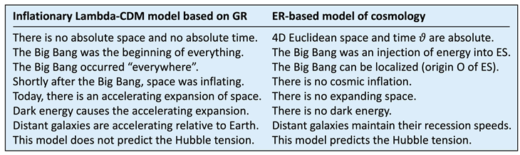
The Hubble tension and cosmological redshift are strong empirical evidence that challenges the Lambda-CDM model. They force us to take a 4D Euclidean geometry into account, and in particular. GR works well when is irrelevant, but of a high-redshift supernova deviates greatly from of the Milky Way. Space is not driven by dark energy. Galaxies are driven by their momentum. Most energy recedes radially from O because of the momentum provided at . Because of various effects (gravity, scattering, photon emission, pair production), some energy does not recede radially anymore. Gravity causes nearby galaxies to move toward our galaxy. Table 1 compares two models of cosmology. ER predicts a whole range of empirical facts, including the Hubble tension. Remarkably, ER manages without cosmic inflation, expanding space, and dark energy. Thus, ER significantly improves cosmology. ER also improves QM (see Section 5.12).
5.12. Quantum Entanglement
Erwin Schrödinger coins the word “entanglement” in a comment [42] on the Einstein–Podolsky–Rosen paradox [43]. These three authors argue that QM does not provide a complete description of reality. Schrödinger’s neologism does not resolve the paradox, but it highlights our enormous difficulties in comprehending QM. John Bell [44] shows that QM is incompatible with local hidden-variable theories. Meanwhile, several experiments [45,46,47] have confirmed that entanglement violates locality in an observer’s 3D space. Quantum entanglement has been interpreted as a “non-local effect” ever since.
Up next, we show: ER “untangles” entanglement without the concept of non-locality. There is no violation of locality in 4D space, where all axes are fully symmetric. In Figure 7, observer R moves along the axis at the speed . We consider two pairs of objects. The first pair was created at the point P and moves in opposite directions (equal to of R). The second pair was created at the point Q and moves in opposite directions . R perceives the first pair as entangled photons and the second pair as entangled material objects, such as electrons. In his 3D space, R perceives each pair as spatially separated objects. He has no idea how they are able to “communicate” with each other in no time.
The photons (or electrons) experience the (or else ) axis as space. For them, the (or else ) axis disappears because of length contraction at the speed . From their perspective, entangled objects have never been spatially separated, yet their proper time flows in opposite 4D directions. This is how they communicate with each other in no time. Their opposite 4D vectors do not affect local communication as long as the twins stay together spatially. Only observers perceive Albert Einstein’s “spooky action at a distance”.
Cosmic homogeneity and entanglement have the same physical background: An observed object’s (or region’s) 4D vector and its 3D space may have rotated with respect to an observer’s 4D vector and his 3D space. This is only possible in ES, where all axes are fully symmetric. The SO(4) symmetry enables the entanglement of photons and other objects [48]. ER predicts that any two objects created in pair production are entangled. This gives us a chance to falsify ER. A measurement terminates one twin or rotates its 4D vector . The entanglement is destroyed. ER manages without non-locality.
6. Conclusions
ER heralds a paradigm shift: (1) Physical realities are projections of a mathematical reality, which is ES. An observer experiences two projections of ES as space and time. As in GR, gravity in ER is the curvature of spacetime. (2) There is an absolute space (ES), an absolute evolution parameter (), and a 4D vector “flow of proper time” (). Information hidden in ES, , and is not available in SR/GR. ES is relevant for modeling an observer’s physical reality. is relevant for modeling galactic motion. is relevant for understanding cosmic homogeneity, cosmological redshift, and entanglement. (3) In ER, is replaced by , and man-made by natural . There is a difference regarding the axis of time dilation. In SR and GR, an observed clock is slow with respect to an observer’s clock in the observed clock’s time axis. In ER, it is slow in the observer’s time axis. Ultimately, this difference is irrelevant because experiments do not reveal in which axis a clock is slow.
ER reproduces the Lorentz factor of SR and the gravitational time dilation of GR. This is not as surprising as it seems. On the one hand, -ST matches the SO(1,3) symmetry of Minkowski spacetime. On the other hand, the EFE are coordinate-invariant and thus also hold in ER. ER refutes the assumption that a background-free approach is advantageous. For instance, time is not an operator in the Schrödinger equation, but acts as an absolute, external parameter. and are such parameters. There are none in SR/GR. In summary, we propose (a) replacing Minkowski spacetime with -ST, (b) using ER in cosmology, and (c) using ER in QM. 12 predicted empirical facts in different (!) areas of physics are most likely not 12 coincidences. Some of these 12 facts can be predicted without ER, but only by postulating cosmic inflation, expanding space, dark energy, and non-locality. ER manages without these concepts. Occam’s razor shaves them all off. No exceptions.
Einstein was awarded the Nobel Prize in Physics 1921 for his theory of the photoelectric effect [49], not for SR or GR. Our results show that ER penetrates to a “deeper level”. Einstein, one of the most brilliant physicists ever, did not realize that nature’s fundamental metric is Euclidean. He sacrificed absolute space and absolute time. ER reinstates absolute space (not 3D space, but 4D space) and absolute time (not a time coordinate, but parameter time). In retrospect, it was man-made coordinate time that delayed the formulation of ER. For the first time, humanity understands the nature of time: Experienced time is the distance traveled in absolute ES divided by . The human brain is able to imagine that we move at the speed of light. Against this backdrop, human conflicts fade into insignificance.
Is ER a physical theory or a metaphysical theory? That is a very good question because we can access ES only in proper coordinates, but we cannot measure the proper time ticking for another object. However, we can calculate from ES diagrams, , and Eqs. (8b) and (15b). ES diagrams are observer-independent Master Diagrams of nature. Observing is our primary source of knowledge, but concepts can mislead us if they originate from observing. Physics is more than just observing. For instance, we cannot observe time. Coordinate time works well in everyday life, but unfortunately has also been applied to the very distant and the very small. For this reason, cosmology and QM benefit most from ER. ER is a physical theory because it predicts what we observe.
It seems as if Greek philosopher Plato anticipated ER in his famous Cave Allegory [50]: Humanity experiences projections, but it cannot observe the Master Reality beyond them. We have laid the foundation for ER and demonstrated its strength. Variational principles can be another way to derive ER, but they are not mandatory. Einstein also derived SR/GR using postulates. One of the most important questions in science is this: How can we describe nature without postulating highly speculative concepts? The answer to this very question leads to the truth. Physics seeks one theory that fits all—from the very distant to the very small. ER is such a theory and is thus indispensable for unifying physics. The projections from ES are also likely to improve our understanding of wave functions in QM. Everyone is invited to test and use ER. Only in ER does Mother Nature reveal her secrets.
Acknowledgments
I thank Siegfried W. Stein for his contributions to Section 5.10 and Figures 2, 4, 5. After several rejections, he decided to withdraw his co-authorship. I thank Felix Finster, Xuan Phuc Nguyen, Dirk Rischke, Jürgen Struckmeier, Christopher Tyler, and Götz Uhrig for asking questions about ER. My special thanks go to all reviewers for investing some of their valuable, proper (!) time.
Comments
(1) Further studies on gravity are required, but this is no reason to reject ER. GR seems to explain gravity, but GR is incompatible with QM unless we add quantum gravity. (2) In ES, there are no singularities and thus no black holes. Again, this is no reason to reject ER. Singularities conflict with QM. Projections of highly concentrated energy could possibly be interpreted as “black holes”. (3) It is often a good idea to match the symmetry. The fundamental symmetry of nature is SO(4). (4) Absolute time puts an end to discussions about time travel. Does any other theory explain time’s arrow as clearly as ER? (5) Physics does not ask: Why is my reality a projection? Projections are far less speculative than postulating cosmic inflation plus expanding space plus dark energy plus non-locality.
It takes open-minded editors and reviewers to evaluate a new theory that heralds a paradigm shift. Taking SR and GR for granted paralyzes progress. I apologize for my numerous preprint versions, but I received little support only. The preprints document my path. The final version is all that is needed. I did not surrender when top journals rejected ER. Interestingly, I was never given any valid arguments that would disprove ER. I was advised to consult experts or submit to other journals. Were the editors afraid of publishing against the mainstream? Did they underestimate the benefits of ER? I was told that predicting 12 empirical facts would be too much to be convincing. I disagree. A paradigm shift often reveals several new insights. Even good friends refused to support me. Every setback motivated me to formulate ER even better. Finally, I identified four shortcomings of coordinate time.
A well-known preprint archive suspended my submission privileges. I was penalized because I showed that GR is not as general as it seems. The editor-in-chief of a top journal replied: “Publishing is for experts only.” One editor rejected ER because it would “demand too much” from his reviewers. Several journals rejected ER because it was “neither innovative nor significant”. I like to speak of ER as “holistic physics”, but unfortunately the reviewers did not accept this term. I do not blame anyone. Paradigm shifts are hard to accept. In the long run, ER will prevail because it predicts what we observe. These comments shall encourage young scientists to stand up for good ideas even if it is challenging: “unscholarly research”, “fake science”, “equations from entry-level textbooks”, “too simple to be true”. Simplicity and truth are not mutually exclusive. Beauty is when they go hand in hand together.
Author Contributions
The entire manuscript was written by the author.
Funding
No funding was received.
Conflicts of Interest
The author has no conflicts to disclose.
Data availability
The data that support the findings of this study are available within this article.
References
- Einstein, A. Zur Elektrodynamik bewegter Körper. Ann. Phys. 1905, 322, 891–921. [Google Scholar] [CrossRef]
- Einstein, A. Die Grundlage der allgemeinen Relativitätstheorie. Ann. Phys. 1905, 354, 769–822. [Google Scholar] [CrossRef]
- Minkowski, H. Die Grundgleichungen für die elektromagnetischen Vorgänge in bewegten Körpern. Math. Ann. 1910, 68, 472–525. [Google Scholar] [CrossRef]
- Rossi, B.; Hall, D.B. Variation of the rate of decay of mesotrons with momentum. Phys. Rev. 1941, 59, 223–228. [Google Scholar] [CrossRef]
- Dyson, F.W.; Eddington, A.S.; Davidson, C. A determination of the deflection of light by the sun’s gravitational field, from observations made at the total eclipse of May 29, 1919. Phil. Trans. R. Soc. A 1920, 220, 291–333. [Google Scholar] [CrossRef]
- Ashby, N. Relativity in the global positioning system. Living Rev. Relativ. 2003, 6, 1–42. [Google Scholar] [CrossRef]
- Ryder, L. Quantum Field Theory; Cambridge University Press: Cambridge, 1985. [Google Scholar]
- Newburgh, R.G., Phipps Jr., T.E.: Physical Sciences Research Papers no. 401. United States Air Force (1969).
- Montanus, H. Special relativity in an absolute Euclidean space-time. Phys. Essays 1991, 4, 350–356. [Google Scholar] [CrossRef]
- Montanus, J.M.C. Proper-time formulation of relativistic dynamics. Found. Phys. 2001, 31, 1357–1400. [Google Scholar] [CrossRef]
- Montanus, H. Proper Time as Fourth Coordinate. 2023. Available online: https://greenbluemath.nl/proper-time-as-fourth-coordinate/ (accessed on 24 May 2026).
- Almeida, J.B. An alternative to Minkowski space-time. arXiv 2001, arXiv:gr. [Google Scholar] [CrossRef]
- Gersten, A. Euclidean special relativity. Found. Phys. 2003, 33, 1237–1251. [Google Scholar] [CrossRef]
- Hudgin, R.H. Coordinate-free relativity. Synthese 1972, 24, 281–297. [Google Scholar] [CrossRef]
- Misner, C.W.; Thorne, K.S.; Wheeler, A. Gravitation; W. H. Freeman and Company: San Francisco, 1973. [Google Scholar]
- Sasane, A. A Mathematical Introduction to General Relativity; World Scientific: Singapore, 2022. [Google Scholar]
- Michelson, A.A.; Morley, E.W. On the relative motion of the Earth and the luminiferous ether. Am. J. Sci. 1887, 34, 333–345. [Google Scholar] [CrossRef]
- Dodelson, S.; Schmidt, F. Modern Cosmology; Elsevier: London, 2025. [Google Scholar]
- Church, A.E.; Bartlett, G.M. Elements of Descriptive Geometry. Part I. Orthographic Projections; American Book Company: New York, 1911. [Google Scholar]
- Nowinski, J.L. Applications of Functional Analysis in Engineering; Plenum Press: New York, 1981. [Google Scholar]
- Wick, G.C. Properties of Bethe-Salpeter wave functions. Phys. Rev. 1954, 96, 1124–1134. [Google Scholar] [CrossRef]
- Matthews, P.C. Vector Calculus; Springer-Verlag: London, 1998. [Google Scholar]
- Hafele, J.C.; Keating, R.E. Around-the-world atomic clocks: predicted relativistic time gains. Science 1972, 177, 166–168. [Google Scholar] [CrossRef] [PubMed]
- Ellis, G.F.R.; Maartens, R.; MacCallum, M. Relativistic Cosmology; Cambridge University Press: Cambridge, 2012. [Google Scholar]
- Oppenheimer, J.R.; Snyder, H. On continued gravitational contraction. Phys. Rev. 1939, 56, 455–459. [Google Scholar] [CrossRef]
- Maxwell, J.C. A dynamical theory of the electromagnetic field. Phil. Trans. R. Soc. 1865, 155, 459–512. [Google Scholar] [CrossRef]
- Abbott, B.P. : Observation of gravitational waves from a binary black hole merger. Phys. Rev. Lett. 2016, 116, 061102. [Google Scholar] [CrossRef]
- Carroll, S.M. Lecture notes on general relativity. arXiv 1997, arXiv:gr. [Google Scholar] [CrossRef]
- Lee, V.S.H.; Zurek, K.M. Proper time observables of general perturbations in laser interferometry-based gravitational wave detectors. Phys. Rev. D. 2025, 111, 124037. [Google Scholar] [CrossRef]
- Ellis, G. The standard cosmological model: achievements and issues. Found. Phys. 2018, 48, 1226–1245. [Google Scholar] [CrossRef]
- Abdalla, E. : Cosmology intertwined: a review of the particle physics, astrophysics, and cosmology associated with the cosmological tensions and anomalies. J. High En. Astrophys. 2022, 34, 49–211. [Google Scholar] [CrossRef]
- Penzias, A.A.; Wilson, R.W. A measurement of excess antenna temperature at 4080 Mc/s. Astrophys. J. 1965, 142, 419–421. [Google Scholar] [CrossRef]
- Hubble, E. A relation between distance and radial velocity among extra-galactic nebulae. Proc. Natl. Acad. Sci. U.S.A. 1965, 15, 168–173. [Google Scholar] [CrossRef]
- Lemaître, G. Un univers homogène de masse constante et de rayon croissant, rendant compte de la vitesse radiale des nébuleuses extra-galactiques. Ann. Soc. Sci. Brux. A 1927, 47, 49–59. [Google Scholar]
- Linde, A. Inflation and Quantum Cosmology; Academic Press: Boston, 1990. [Google Scholar]
- Guth, A. The Inflationary Universe; Perseus Books: New York, 1997. [Google Scholar]
- Aghanim, N. : Planck 2018 results. VI. Cosmological parameters. Astron. Astrophys. 2020, 641, A6. [Google Scholar]
- Riess, A.G. : A comprehensive measurement of the local value of the Hubble constant with 1 km s−1 Mpc−1 uncertainty from the Hubble Space Telescope and the SH0ES team. Astrophys. J. Lett. 2022, 934, L7. [Google Scholar] [CrossRef]
- Perlmutter, S. : Measurements of Ω and Λ from 42 high-redshift supernovae. Astrophys. J. 1999, 517, 565–586. [Google Scholar] [CrossRef]
- Riess, A.G. : Observational evidence from supernovae for an accelerating universe and a cosmological constant. Astron. J. 1998, 116, 1009–1038. [Google Scholar] [CrossRef]
- Turner, M. Dark matter and dark energy in the universe. arXiv 1998, arXiv:astro. [Google Scholar] [CrossRef]
- Schrödinger, E. Die gegenwärtige Situation in der Quantenmechanik. Naturwissenschaften 1935, 23, 807–812. [Google Scholar] [CrossRef]
- Einstein, A.; Podolsky, B.; Rosen, N. Can quantum-mechanical description of physical reality be considered complete? Phys. Rev. 1935, 47, 777–780. [Google Scholar] [CrossRef]
- Bell, J.S. On the Einstein Podolsky Rosen paradox. Physics 1964, 1, 195–200. [Google Scholar] [CrossRef]
- Freedman, S.J.; Clauser, J.F. Experimental test of local hidden-variable theories. Phys. Rev. Lett. 1972, 28, 938–941. [Google Scholar] [CrossRef]
- Aspect, A.; Dalibard, J.; Roger, G. Experimental test of Bell’s inequalities using time-varying analyzers. Phys. Rev. Lett. 1982, 49, 1804–1807. [Google Scholar] [CrossRef]
- Bouwmeester, D. : Experimental quantum teleportation. Nature 1997, 390, 575–579. [Google Scholar] [CrossRef]
- Hensen, B. : Loophole-free Bell inequality violation using electron spins separated by 1.3 kilometres. Nature 2015, 526, 682–686. [Google Scholar] [CrossRef]
- Einstein, A. Über einen die Erzeugung und Verwandlung des Lichtes betreffenden heuristischen Gesichtspunkt. Ann. Phys. 1905, 322, 132–148. [Google Scholar] [CrossRef]
- Plato. Politeia; p. 514a.
Figure 1.
Minkowski diagram and ES diagram of two uniformly moving clocks. Left: “b” is slow with respect to “r” in . Coordinate time is relative (“b” is at different positions in and ). Right: “b” is slow with respect to “r” in . The evolution parameter is absolute (both clocks are at ).
Figure 1.
Minkowski diagram and ES diagram of two uniformly moving clocks. Left: “b” is slow with respect to “r” in . Coordinate time is relative (“b” is at different positions in and ). Right: “b” is slow with respect to “r” in . The evolution parameter is absolute (both clocks are at ).
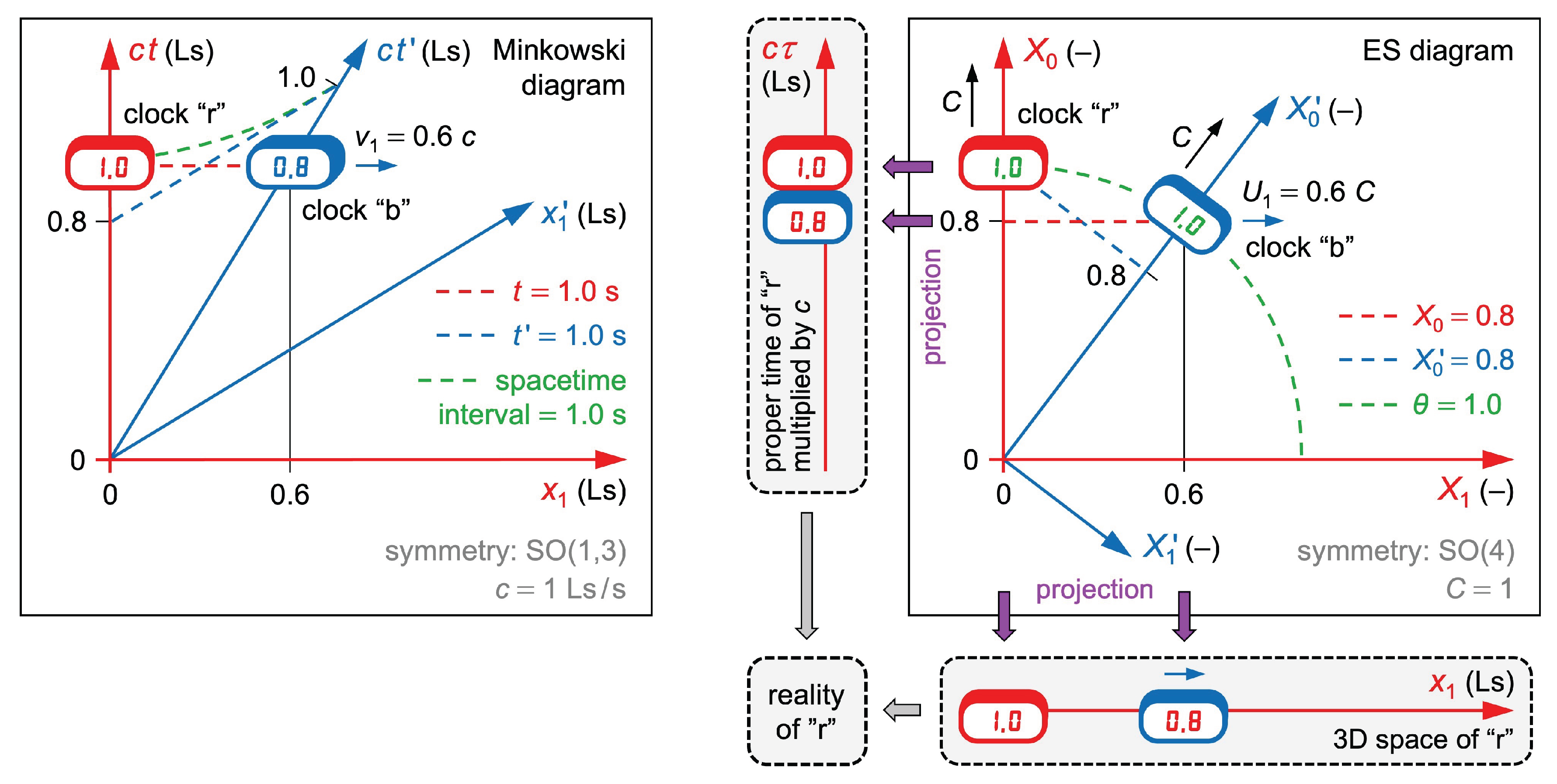
Figure 2.
ES diagrams of two uniformly moving rockets. “r” and “b” move in different 4D directions. The ES diagrams are identical. Bottom left: In the projection onto the 3D space of R, “b” contracts to . Bottom right: In the projection onto the 3D space of B, “r” contracts to .
Figure 2.
ES diagrams of two uniformly moving rockets. “r” and “b” move in different 4D directions. The ES diagrams are identical. Bottom left: In the projection onto the 3D space of R, “b” contracts to . Bottom right: In the projection onto the 3D space of B, “r” contracts to .
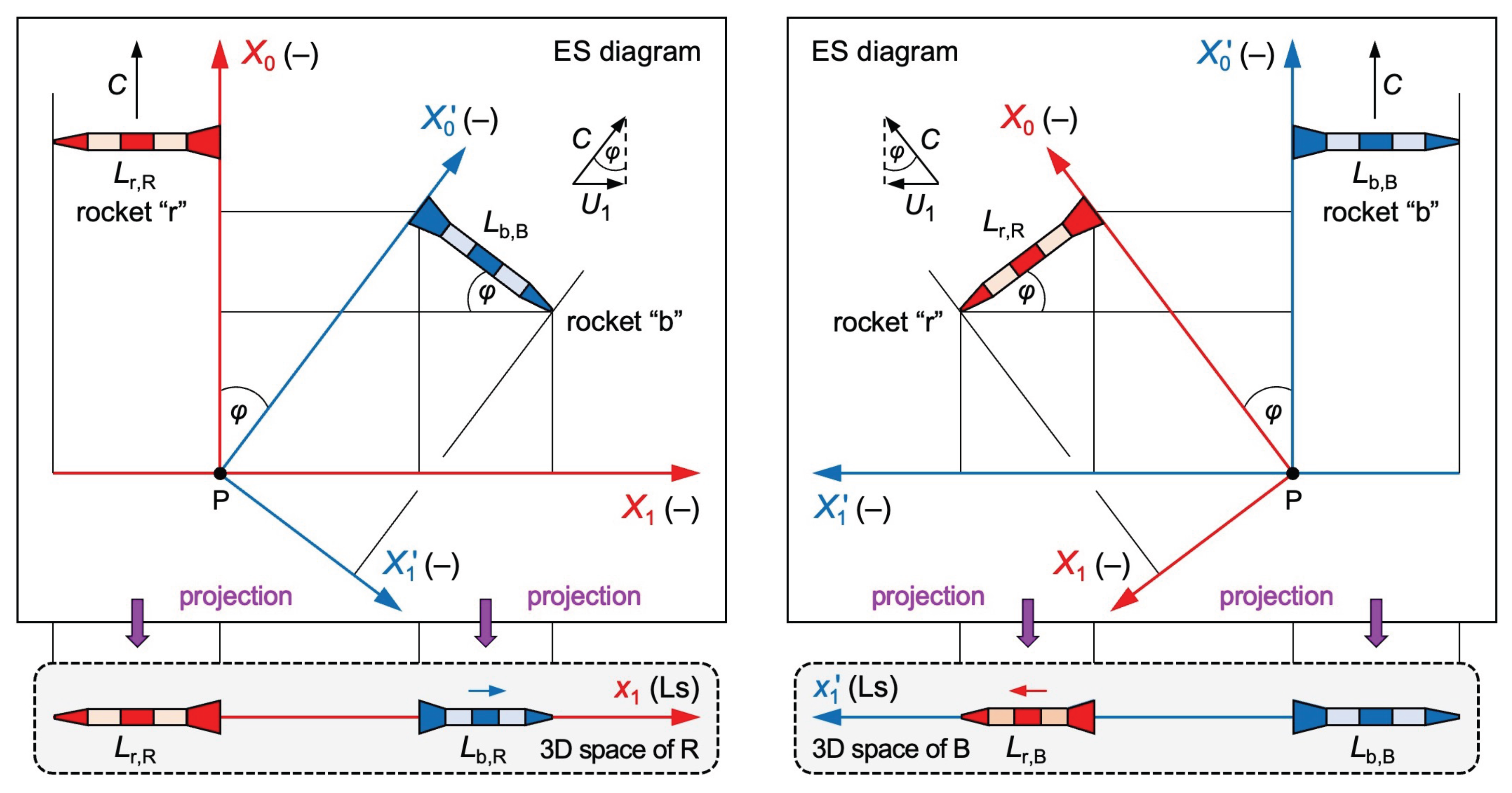
Figure 3.
Clock “b” falls freely toward Earth. Left: indicates the current 4D motion of “b”. In the 3D space of “r”, “b” accelerates toward Earth. Right: This is not an ES diagram. “b” experiences gravity as an acceleration of everything else. In the 3D space of “b”, Earth accelerates toward “b”.
Figure 3.
Clock “b” falls freely toward Earth. Left: indicates the current 4D motion of “b”. In the 3D space of “r”, “b” accelerates toward Earth. Right: This is not an ES diagram. “b” experiences gravity as an acceleration of everything else. In the 3D space of “b”, Earth accelerates toward “b”.
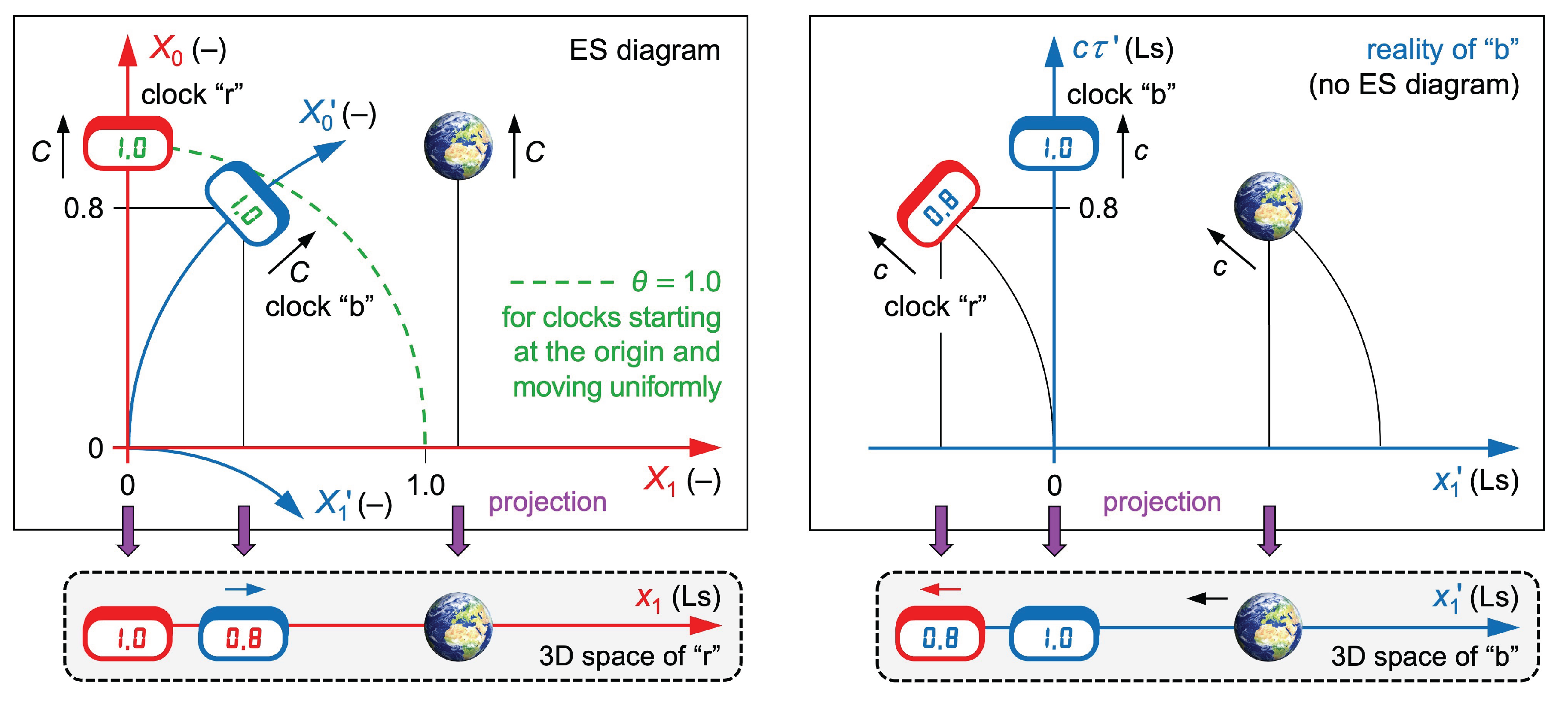
Figure 4.
Instructive problems. Left: In the 3D space of a guide wire, a rocket moves along the wire. In ES, the wire escapes from the rocket. Right: In the 3D space of the sun, Earth orbits the sun. In ES, the sun escapes from Earth. We ignore the fact that the sun orbits the center of the Milky Way.
Figure 4.
Instructive problems. Left: In the 3D space of a guide wire, a rocket moves along the wire. In ES, the wire escapes from the rocket. Right: In the 3D space of the sun, Earth orbits the sun. In ES, the sun escapes from Earth. We ignore the fact that the sun orbits the center of the Milky Way.
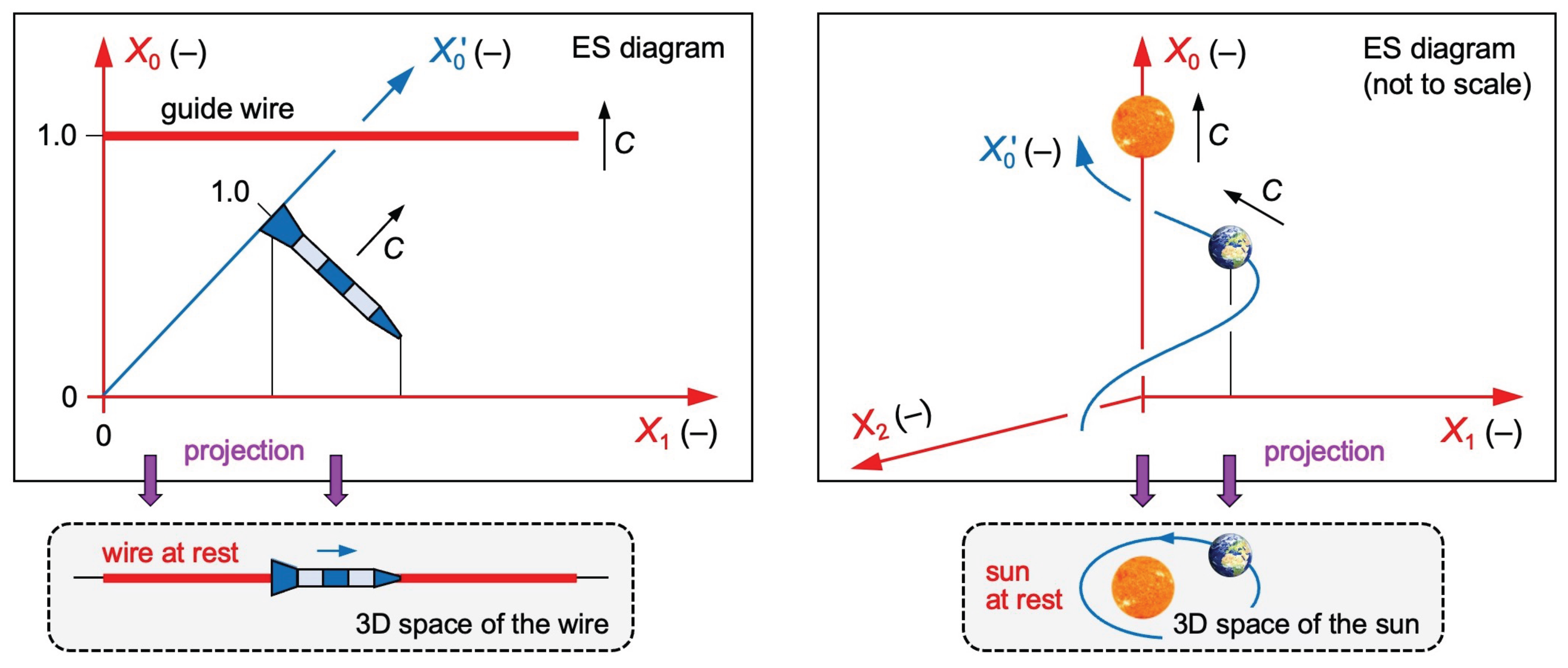
Figure 5.
ER-based model of cosmology. Left: A galaxy G recedes from the origin O at the speed and from the axis at the speed . Right: If a star happens to be at the same distance today at which the supernova of S occurred, recedes more slowly from the axis than S.
Figure 5.
ER-based model of cosmology. Left: A galaxy G recedes from the origin O at the speed and from the axis at the speed . Right: If a star happens to be at the same distance today at which the supernova of S occurred, recedes more slowly from the axis than S.
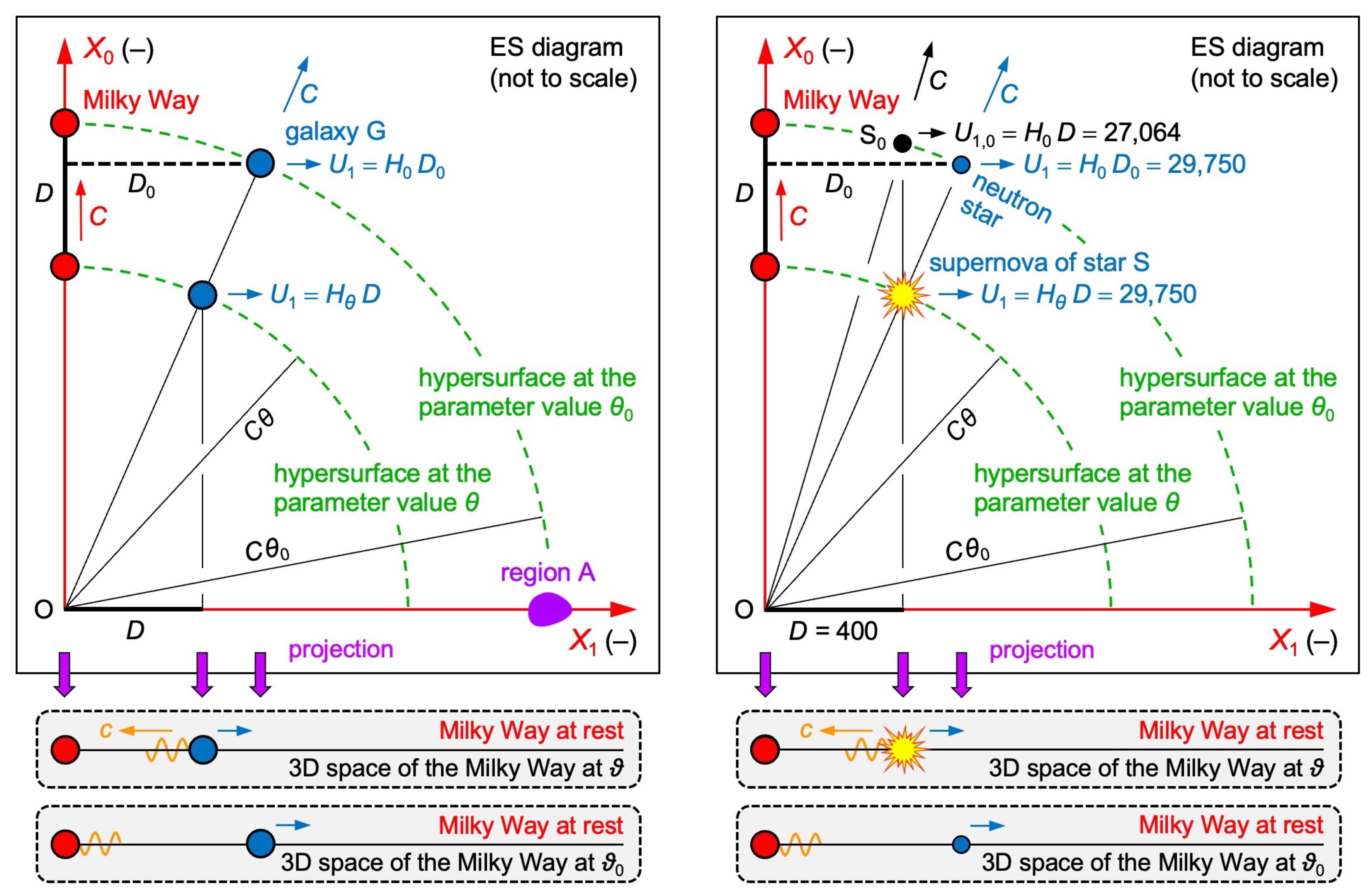
Figure 6.
Hubble diagram of simulated supernovae. According to Eqs. (27) and (30), the recession speed is equal to . Thus, the red points do not form a straight line. According to Eq. (29), the recession speed is equal to . Thus, the blue points do form a straight line.
Figure 6.
Hubble diagram of simulated supernovae. According to Eqs. (27) and (30), the recession speed is equal to . Thus, the red points do not form a straight line. According to Eq. (29), the recession speed is equal to . Thus, the blue points do form a straight line.
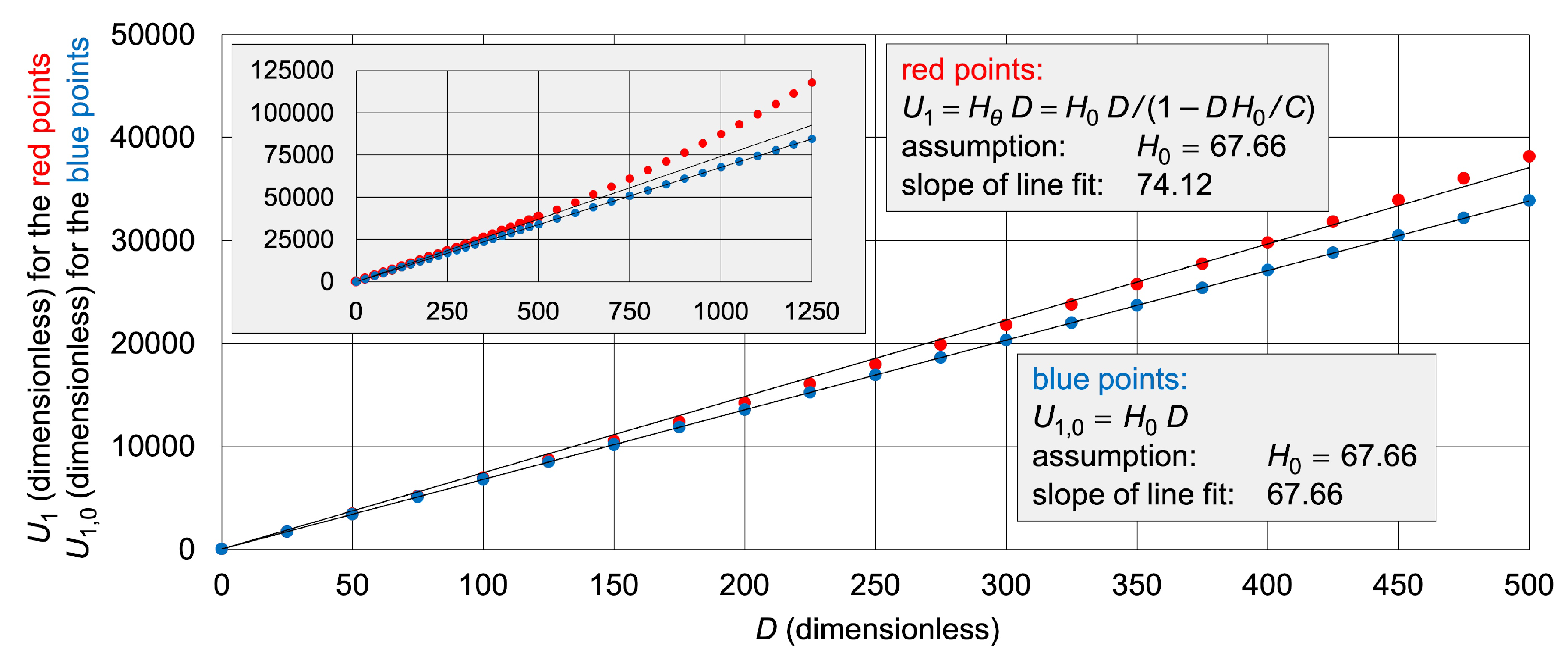
Figure 7.
Entanglement. R moves along the axis. He experiences the axis as space. In his 3D space, R perceives entangled objects as spatially separated objects. The photons (or electrons) experience the (or else ) axis as space. In their 3D space, entangled objects stay together spatially.
Figure 7.
Entanglement. R moves along the axis. He experiences the axis as space. In his 3D space, R perceives entangled objects as spatially separated objects. The photons (or electrons) experience the (or else ) axis as space. In their 3D space, entangled objects stay together spatially.
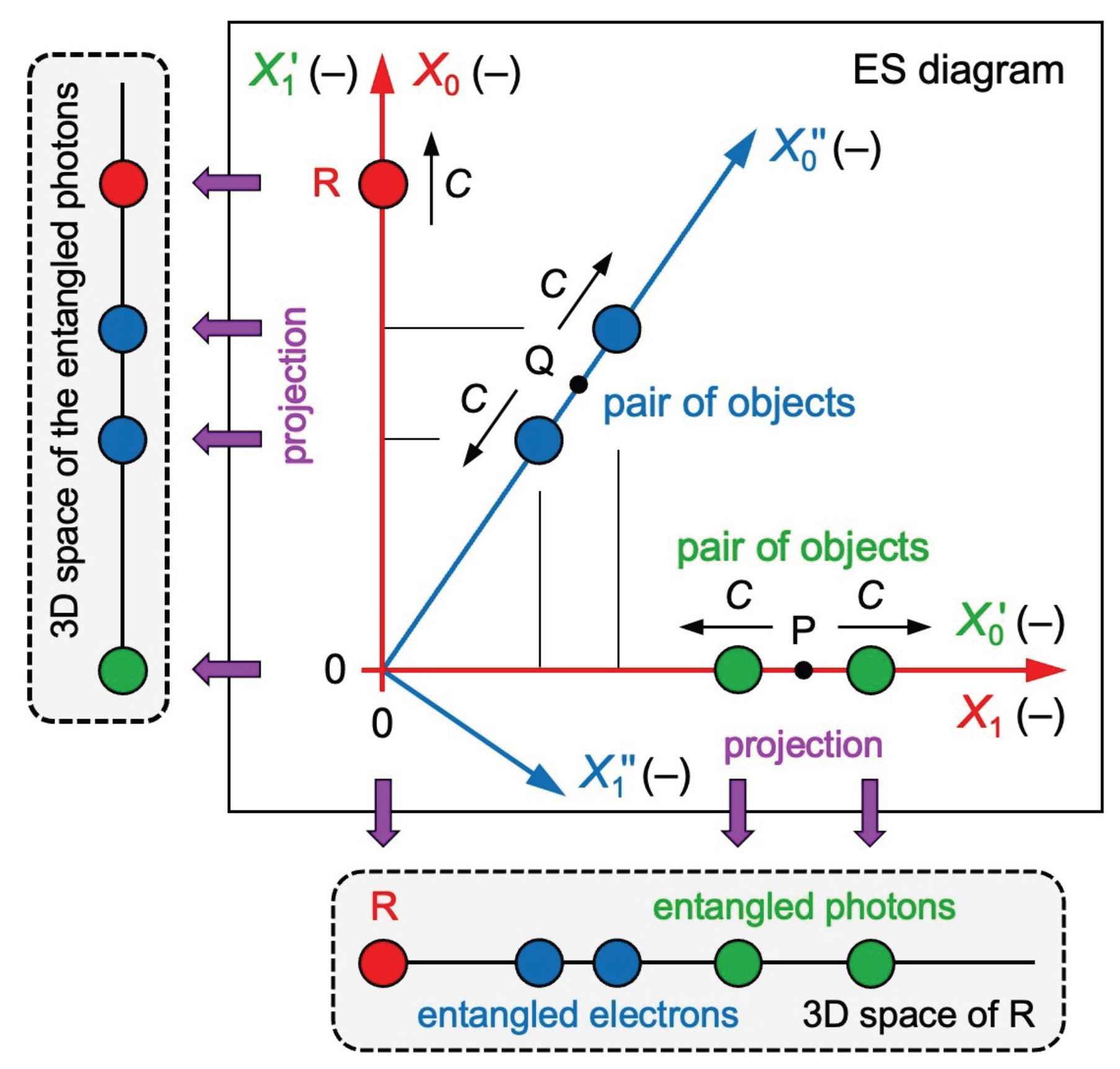

Table 1.
Comparing two models of cosmology.
 |
Disclaimer/Publisher’s Note: The statements, opinions and data contained in all publications are solely those of the individual author(s) and contributor(s) and not of MDPI and/or the editor(s). MDPI and/or the editor(s) disclaim responsibility for any injury to people or property resulting from any ideas, methods, instructions or products referred to in the content. |
© 2026 by the authors. Licensee MDPI, Basel, Switzerland. This article is an open access article distributed under the terms and conditions of the Creative Commons Attribution (CC BY) license (http://creativecommons.org/licenses/by/4.0/).
Copyright: This open access article is published under a Creative Commons CC BY 4.0 license, which permit the free download, distribution, and reuse, provided that the author and preprint are cited in any reuse.


