
Submitted:
25 January 2023
Posted:
26 January 2023
You are already at the latest version
Abstract
The analogy between the theory of phase transitions in simple fluids and vehicular traffic flow has long been suspected, promising a new level of understanding of urban congestion by standing on one of the firmer foundations in physics. The obstacle has been the interpretation of the thermal energy of the gas-particle system, which remains unknown. This paper proposes the flow of cars through the network as a viable interpretation, where the fundamental diagram for traffic flow would be analogous to the coexistence curve in gas-liquid phase transitions. Thanks to the power-law form of the coexistence curve, it was possible to formalize that the resulting network traffic model belongs to the Kardar-Parisi-Zhang universality class. The scaling relationships arising in this universality class are found to be consistent with West's scaling theory for cities. It is shown that congestion costs (delays + fuel consumption) scale superlinearly with city population, possibly and worryingly more so than predicted by West's theory. Implications for sustainability and resiliency are discussed.
Keywords:
Urban congestion
; Traffic flow theory
; Phase transitions
; KPZ universality class
; Nonequilibrium physics
The remarkable scaling theory for cities [1,2,3,4] proposed by West and coworkers indicates that urban transportation networks are analogous to biological networks inside organisms transporting the energy to survive. As such, urban networks exhibit economies of scale when it comes to infrastructure needs; e.g., doubling the population of a city requires only about 1.8 times the number of gas stations, lane-miles of road, etc. Unlike biological networks, however, the social interactions taking place in cities produces about 2.2 times the wages, number of patents, crime and, as we will see here, traffic congestion costs. This is not good news for traffic congestion going forward, but this paper gives new insights into these growth mechanisms to better understand how to curb it.
Urban networks are the perfect example of simple local rules producing what appears to be complicated, chaotic and unpredictable dynamics. Indeed, the rules of traffic flow are exceedingly simple: “Advance if you can", yet its consequences can be very frustrating for the average commuter. An explanation for these unpredictable dynamics has long been conjectured [5] based on percolation phase transitions and self-organized criticality. They show that the lifetime of traffic jams can be arbitrarily large as they obey a power-law distribution near the critical density. Power laws are the hallmark of fractal objects and complex systems having phase transitions, and due to their infinite variance are responsible for the chaotic and unpredictable dynamics. Fig. Figure 1 shows these power-law dynamics in action on a single lane of traffic. When the density of cars, , is slightly larger than the critical density, , the jam clusters, which contains only bumper-two-bumper vehicles, percolate upstream (in the opposite traffic direction) eventually spilling over to the rest of the network. But if the density is slightly smaller, it is the traffic voids that percolate downstream. This strong dependence on initial conditions is what makes prediction challenging. Notice the self-similarity of the different triangles in the figure, revealing the fractal nature of traffic. Recent studies reveal power-law distributions for the jam clusters in Fig. Figure 1 [6], the average platoon size and the average speed of vehicles [7] and the relaxation to stationary state [8].
But a traffic theory based on the analogy with phase transitions is still lacking [9,10,11,12]. Two decades ago in an excellent review of traffic flow models, Nagel et al [12] conjecture that such an analogy would set traffic flow theory on one of the firmer foundations in physics, offering a coherent description from the microscopic driver behavior to the macroscopic system dynamics. The only obstacle seems to be the interpretation of thermal energy. Quoting [12]: “[...]once one has identified the traffic model parameter that corresponds to temperature, then some good analogy between the gas-liquid transition and laminar-jammed transition seems to be possible. However, without identification of that parameter, characterization of models is difficult.”
The two-fluid model of Prigogine and Herman [13], based on their kinetic theory of vehicular traffic [14], was a first attempt in this direction. They interpreted the temperature as the speed of vehicles, but the analogy with phase transitions is only formal [15], and it does not allow descriptions at different scales. They made the important observation, embraced in this paper, that at a fundamental level traffic flow has only two phases: a gas phase where vehicles are moving and a liquid phase where vehicles are stopped.
This paper shows that interpreting the thermal energy of the particle system as the flow of cars through the network makes it possible to formulate a theory in complete analogy with the gas-liquid equilibrium phase transitions. This analogy is described by a single parameter, the order-parameter critical exponent in the theory of phase transitions, which is found to have several important interpretations, each discussed in the following sections of this paper: as the maximum throughput (capacity) of the network, as the aggregation level, as the nonlinear-term constant in the KPZ equation, and as the normalizing constant for congestion delays.
1. The liquid-gas coexistence curve
Phase transitions are characterized by an order parameter, the number density of molecules (cars) in our case, whose critical value, , separates the ordered phase (liquid/congestion) and of the disordered phase (gas/free-flow). Near the critical density most quantities of interest obey a power-law relationship of the reduced temperature , where the critical temperature depends on the specific fluid. In thermal equilibrium, the coexistence curve:
bounds a compact region in the density-temperature plane where the phase transition occurs, i.e. where the proportion of matter in one phase increases gradually from 0 to 1. An example of this coexistence curve was observed empirically by Guggenheim in 1945 for 8 simple fluids [16] as an example of the “principle of corresponding states” in chemistry. This principle can be seen as a precursor of the remarkable concept of universality classes in statistical mechanics, which groups physical systems sharing the same critical exponents. Simple fluids and ferromagnets have been known to obey since the 1890’s [17], and more recently they are said to belong to the Ising universality class [18].
Fig. Figure 2 illustrates the coexistence curve for 77 simple fluids. It exhibits a remarkable low scatter as a consequence of universality. Notice that (1) is symmetric with respect to the critical density, but the coexistence curve is not. To circumvent this one can make the shape of coexistence curves mirror-symmetric with respect to the line , by applying the shear mapping described in [23] and summarized in the Appendix. This mapping is illustrated in Fig. Figure 2, where it has been applied to the entire left panel of the figure to make the point. Notice the remarkable agreement with the data of (1) using over the entire density range after the transformation (right panel). In practical terms this means that one may always assume the coexistence curve to be symmetric with
which is the assumption hereafter in the paper.
1.1. The fundamental diagram (FD) of traffic flow
The FD gives the equilibrium relationship between any pair of traffic variables, typically flow (or current) f, density and speed v, describing the motion of cars in a particular one-dimensional link in the network. Here the normalized flow of traffic, , is interpreted as being proportional to the temperature in the coexistence curve (1). The Appendix makes this interpretation more precise. To derive the equation of the FD, solve for in (1) to get , or better still to ensure zero flow for empty and jam-density conditions, i.e. . Therefore:
where the prefactor –which corresponds to the maximum flow or capacity of the facility–ensures that both the free-flow and congestion wave speeds are always unity regardless of the value of , i.e. ; see Fig. Figure 3. This makes the only parameter needed to fully describe traffic flow in equilibrium.
1.2. The microscopic traffic model and different aggregation levels
When the FD becomes an isosceles-triangle; see Fig. Figure 3. Triangular diagrams embody the simplest microscopic rules: “Travel at the free-flow speed unless impeded by the downstream car”. These rules are the basis for the influential Nagel-Schreckenberg (NaSch) model [25] which adds stochastic fluctuations by introducing the probability of slowing down by one speed unit for moving vehicles. But because the shape of the triangular diagram is irrelevant thanks to the shear symmetry discussed above, one can choose giving the isosceles triangle in Fig. Figure 3 without loss of generality. This means that the celebrated Newell’s car-following model [26], which can be formulated as a cellular automaton [27], is equivalent to elementary cellular automata rule 184 [28], which in turn is equivalent to the totally asymmetric simple exclusion process (TASEP), for which many exact results are known. All experimental results in the remainder of the paper use the NaSch model with , and it will be simply referred to as the “traffic model”.
Vehicle trajectories, either real or generated by the traffic model, can be aggregated at different levels. [24] derived the lane-level FD based on results from TASEP for , which gives the steady-state average flow on a single circular lane of length L with a constant density of vehicles. They found that the capacity in this case is , which means that at the link-level we have:
The dashed lines in Fig. Figure 3 depict the lane-level FD assuming (4). It can be seen that the agreement with the proposed FD is exact for , and that it deteriorates for except near the critical density. The Appendix shows that reasonable values for the slowdown probability should satisfy , and we conclude from (4) that is a reasonable interval at the lane-level FD.
At the network-level, the macroscopic FD (MFD) [29] gives the average flow versus average density, the average taken across all links in the network under steady-state conditions. It has received much attention during the last decade as an efficient way to control urban traffic [30,31,32,33]. The insets in Fig. Figure 2(right) show empirical MFDs of vehicular traffic for different European cities, where it can be seen that the proposed FD (3) provides a good fit with , depending on the city. Keep in mind that this results have to be taken with a grain of salt because of unresolved challenges in the experimental observation of the MFD: traffic conditions are seldom in steady-state across the network, traffic counts are typically available from detectors only in a subset of the links, and detector location within the link can have an important impact in the flow-density estimations. The insets in the left panel of the figure shows empirical MFDs for pedestrian traffic, which are devoid of these challenges and therefore more reliable. Notice how the value of is highly correlated with the directionality of pedestrian traffic.
2. Dynamic deterministic behavior
The description of traffic flow through the FD is an equilibrium one, valid only when the system is in steady state. Dynamic behavior can be extracted by adding the conservation law of vehicles on the road: , known as the kinematic wave or LWR model [34,35], an has played a central role in traffic science to this day. An alternative formulation of this model that turns out to scale nicely to the stochastic case in the next section, is achieved using Newell’s traffic flow surface [36,37], , that gives the cumulative number of vehicles having crossed location x by time t, starting from the passage of a reference vehicle. Its gradients are given by densities and flows: , which means that the very existence of the FD implies
a Hamilton-Jacoby partial differential equation (PDE), whose solutions can be found by solving the shortest path problem:
known as the Hopfs-Lax formula [38]. In this variational formulation the FD corresponds to the Hamiltonian of the system, whose corresponding Lagrangian is denoted [39,40]. The shortest path problem consists in finding a trajectory from to the initial (and/or boundary) data at that minimizes the total cost along the path, given by the term in brackets. As shown next, the noisy version of this minimum path problem is at the heart of a wide variety of dynamical systems with the same scaling properties.
3. Stochastic nonequilibrium behavior
It is well-known that random fluctuations have important impacts on systems in one spatial dimension, such as the one studied here, and therefore mean-field approximations are bound to fail. Nonequilibrium physics has made important advances in the last two decades to understand these impacts by formalizing the existence of dynamical universality classes [41,42,43]. The Gaussian universality class is the best-known due to the ubiquity of the central limit theorem. It is embodied in the Brownian motion stochastic process, which typically applies in non-interacting particle systems, where particle positions/states are independent of each other, and therefore normally distributed with fluctuations (i.e. standard deviation) growing as . But most complex random systems do not follow fall into this universality class due to spatial correlations from the interactions among nearby particles. These systems are believed to be in the Kardar-Parisi-Zhang (KPZ) universality class [44], where fluctuations grow only as [45], and obey, instead of the normal distribution and Brownian motions, a distribution/process that depends on the initial conditions; see Table 1. This dependence comes from the number of possible candidate solutions to (a noisy version of) (6), which varies depending on the initial condition, with the shortest path cost given by the Tracy-Widom distributions [46]. These distributions [47,48] play a key role in this universality class, and appears in a wide variety of fields including random matrix theory, queuing theory, shortest path on random media, combinatorics, surface growth models, big data regression models and many others [45,49]. This speaks to the remarkable breath and depth of KPZ universality, with new members being added regularly. The KPZ equation is the stochastic PDE member of this class, which is typically formulated in terms of a surface, , representing the height of the interface of growth processes:
where is a surface tension responsible for the particle relaxation/diffusion at the surface, controls the strength of the nonlinear term, and is a Gaussian space-time white noise with zero mean and variance (or diffusion coefficient) .
That traffic flow belongs to the KPZ universality class is a conjecture at the moment, and it is the purpose of this section to strengthen the case. This conjecture was proven in [24] for the NaSch model with and for all values of the slowdown probability . They also showed this numerically for , which we are in a position to prove here thanks to the shear mapping introduced in Section 1, whereby the shape of a triangular diagram is irrelevant and so is the value of . In addition, they showed by simulation that this conjecture also applies in multilane roads with lane changes, which gives a strong indication that this conjecture might be true in general.
An additional argument to support this conjecture is based on the existence of the FD, , which implies (5) in the deterministic case. As in the KPZ equation, one can add viscosity and random noise for generality:
A second-order Taylor series expansion of f around a stationary density does give the KPZ equation, but unfortunately this comes with the condition ; see [24]. This condition might be too restrictive in the case of traffic flow since it is commonly found that is either or exhibits a singularity (as in our case (3)) near the critical density, which is the main interest here.
It turns out that for the FD proposed here (3) this restriction disappears if one defines
i.e. the fluctuations are the deviations of Newell’s traffic surface with respect to the deterministic solution in (6). The Appendix shows these deterministic solutions for important initial conditions; for flat initial conditions, which represent cars flowing at the critical density uninterrupted by bottlenecks, we have per (A4). Substituting (9) in (8) gives:
which is exactly the KPZ equation (7) with for . For other values of we have a generalized nonlinearity and (, which reveals yet another interpretation of the critical exponent ). Fortunately, the exact type of nonlinearity is not crucial when it comes to KPZ universality [44,56]; see the Appendix. The Appendix also shows that (10) follows for step initial conditions, which represent the flow out of bottlenecks, such as traffic signals. This means that both interrupted and uninterrupted traffic are part of the KPZ class.
To give a visual intuition why traffic flow belongs to the KPZ universality class, Fig. Figure 4 shows the fluctuation surface per (9) produced by the NaSch model with Brownian motion initial conditions and different stopping probabilities . Notice how the fluctuation magnitude decreases with time, as expected from KPZ where they behave as instead of in uncorrelated flows. In the stochastic case the surface resembles a natural landscape, in agreement with Newell [37] who noted that the variational formulation of traffic flow is similar to soil erosion models, which also appear to be KPZ universal [57].
4. Scaling of traffic congestion
An important consequence of KPZ universality is that, in the long run, important variables having units of time, scale with the total lane-miles of the network as , where the dynamical exponent z equals 3/2 in KPZ. Therefore, one expects that for large times, large transportation networks will exhibit such scaling behavior for the travel delay as a consequence of congestion, . In the case of our traffic model, the delay is simply the total size of jam clusters, see Fig. Figure 1. Surprisingly, it appears that the scaling relationship
is valid in general, not only in the large-scale limit. It was recently shown in [6] that even for a single one-lane road (where ) (11) holds exactly for the deterministic traffic model with white noise initial conditions. This result is based on the correspondence between delay and the area under the Brownian motion corresponding to the initial conditions, which are known to scale as and to obey the Airy distribution [58,59,60]; see Fig. Figure 4(top). In the case of the stochastic traffic model, Fig. Figure 5 (left) shows that (11) applies in the physically relevant case . Notice that the different curves for different stopping probabilities tend to overlap for as shown in the inset, with given by (4), revealing yet another interpretation of this parameter as the natural units to measure delay.
Although empirical data on and to validate (11) are not readily available, one can use the delay and population, M, estimates from the Urban Mobility Report [61] shown in Fig. Figure 5 (right), by expressing (11) in terms of the city population. The fractal properties of urban network topology imply , where is the fractal dimension of the transportation network and A is the urbanized area of the city [62,63,64]. Assuming that the urbanized area scales linearly with population, i.e. as suggested by Fig. Figure 5 (right), we get:
In a first-order approximation the value of in this equation is the average network fractal dimension, , across the 500 cities in the data set. This can be estimated using the relationship found in [63] for the Dallas Fort Worth area, which gives and the slope matches the data in Fig. Figure 5 (right). It can be shown that the second-order approximation gives a slope of 1.27. Alternatively, we can use the network fractal dimensions reported in [64] for the largest 95 metro areas in the United States, which gives first- and second-order approximations for the slope of 1.11 and 1.14, respectively.
This last estimate is an excellent agreement with West’s scaling theory for cities mentioned in the introduction, which predicts a slope of 1.15 for most externalities of urban living including wages, city GDP, number of patents, and crime. Based on the results in this section, it appears that congestion delays also follow this superlinear scaling law possibly with a larger slope of around 1.2 as suggested by the data. Although not shown here for brevity, the same data [61] reveals that the excess fuel consumed produces a chart almost identical to Fig. Figure 5(right) with a slope also around 1.2. This is consistent with the definition of excess fuel being consumed during the delay component of travel time, and therefore should scale similarly.
5. Discussion and outlook
It would be interesting to see if the thermodynamics analogy proposed in this paper is sufficient to allow the theory of critical phenomena and phase transitions to be used in solving urban congestion problems, as conjectured by Nagel et al [12] two decades ago. This would be a major milestone not only for urban congestion control and planning, but for many related complex systems with power-law dynamics. Elsewhere we will show that heat corresponds to Newell’s traffic surface, temperature to network production, and entropy to travel time, and that the second law of thermodynamics in this case means that travel times tend to increase near the critical density. To complete the description, the potential energy should be taken as the remaining distance to the destination, where particles rest, possibly including departure and arrival time penalties.
While fluids in thermal equilibrium belong to the Ising universality class, traffic does not because of its anisotropic behavior. The directed percolation universality class appears as a strong candidate, considering that its value for accords well with the empirical network-level FDs in Fig. Figure 2. This is an agreement with recent empirical observations which also suggest direct percolation as the universality class of urban networks [66]. Far from equilibrium, we concluded that traffic flow near the critical density belongs to the KPZ universality class, as a consequence of the nonlinearity of the FD. This result should also apply for supply chains given the mathematical similarities [67], and extend naturally to other systems of conservation laws with power-law dynamics.
An immediate consequence of KPZ universality is the scaling of congestion costs of delays plus fuel consumption, revealing a superlinear scaling with respect to population that is in line with West’s scaling theory for cities. This is problematic as it indicates that doubling the population of a city will more-than-double congestion costs, i.e. by a factor of according to West’s theory or as shown here. The exponent in (11) with for the KPZ class, indicates that more sustainable growth could be afforded by lowering the dynamical critical exponent z and-or the network fractal dimension . Research is needed to devise mechanisms to lower z; other known universality classes arising from the interaction conservation laws is the Fibonacci family [42], but their dynamical exponents are all and tend to the Golden ratio . Lowering the network fractal dimension appears easier to achieve in practice, possibly at the expense of lower connectivity. This suggests that there may be an optimal level of connectivity that strikes a balance between mobility and sustainability, which remains to be explored. Traffic control is unlikely to alter the scaling relationship (11), but it can help with network resilience: Because traffic flow is naturally driven to be in the critical state that maximizes throughput, it exhibits self-organized criticality [68], where the system becomes more and more fragile in the process. As it reaches this state of maximum throughput, the entire system performance can collapse for no apparent reason due to the power-law dynamics taking place [5,6,69]. Resiliency can be improved by designing control strategies that prevent reaching the critical state, but without significant impacts in delays. These are all important questions that will hopefully find answers soon to improve the livability of cities going forward.
Acknowledgments
This research was partially funded by NSF Awards #1932451, #1826003 and by the TOMNET University Transportation Center at Georgia Tech.
Appendix
Appendix A.1. Fluid data for Figure 2
The temperature-density data for the simple fluids in Figure 2 were obtained using the function ThermodynamicData[] in Mathematica [70]. The list of the 77 fluids in Fig. 2 is: Acetone, Ammonia, Argon, Benzene, Butane, Butene, Carbon Dioxide, Carbon Monoxide, Carbonyl Sulfide, Cis Butene, Cyclohexane, Cyclopropane, Decane, Dodecane, Ethane, Ethanol, Ethylene, Fluorine, Heptane, Hexane, Hydrogen Sulfide, Isobutene, Isohexane, Isopentane, Krypton, Methane, Methanol, Neon, Neopentane, Nitrogen, Nitrogen Trifluoride, Nitrous Oxide, Nonane, Octane, Oxygen, Pentane, Perfluoropentane, Propylene, R11, R113, R114, R116, R12, R123, R124, R125, R13, R134a, R14, R141b, R142b, R143a, R152a, R21, R218, R22, R227ea, R23, R236ea, R236fa, R245ca, R245fa, R32, R365mfc, R41, RC318, Sulfur Dioxide, Sulfur Hexafluoride, Toluene, Trans Butene, Trifluoroiodomethane, Water and Xenon.
Appendix A.2. The forgotten symmetry
The well-known Galilean transformation expresses the invariance of the physical world to inertial frames of reference moving at a constant velocity , and leaves a conservation law identical. A lesser-used linear symmetry that leaves conservation laws invariant is the shear (or skewing or transvection) mapping:
which can be interpreted as using asynchronous time, where clocks start running at each location according to the passage of an observer moving at a constant velocity . In conjunction with
leaves also delays and total distance traveled unchanged; see [23] for details. The significance of the shear mapping (A1)-(A2) is that one can make the shape of coexistence curves mirror-symmetric with respect to the line by using . This mirror-symmetry guarantees that the critical exponent is indeed the same at either sides of the critical point, an assumption typically made in the phase transitions literature, which now finds a solid justification. In physical chemistry the line of symmetry for coexistence curves (connecting the critical point to ) is known as the diameter and has been used to improve the estimations of the critical point by assuming that it is in fact rectilinear [71]. Although it appears that no connections with the shear mapping have been made, the benefits of having a symmetrical coexistence curve were clear to this community who devised different methods to approximate it [72,73].
Appendix A.3. Flow ∝ temperature ∝ heat flow in equilibrium
It is important to point out that interpreting the flow of vehicles as the temperature is only valid in equilibrium. More rigorously, the flow is interpreted here as the heat flow, which gives the rate of heat transfer per unit time. By Fourier’s law of thermal conduction the heat flow is proportional to the temperature gradient in the system. But for simple homogenous systems in thermal equilibrium, the temperature gradient is, in turn, proportional to the temperature alone [74].
Appendix A.4. Why the slowdown probability should be p s <0.1
To see this, consider a single vehicle driving on an empty lane according to the NaSch model; i.e. at each time step it drives with a free-flow speed of 1 with probability or it stops with probability . It follows that the speed at each time step is a Bernoulli random variable with parameter , whose coefficient of variation is . Using the rule of thumb of keeping this coefficient under 30 percent gives and the claim follows.
Appendix A.5. Deterministic solutions for flat and step initial conditions
The fundamental diagram corresponds to the Hamiltonian of the system, whose Legendre-Fenchel transform gives the Lagrangian. For the proposed fundamental diagram (3) the Lagrangian is given by:
where is a wave speed and the sign % means ”same as in line above”. Since the Lagrangian is independent of space and time, the solution of (6) is greatly simplified. The time integral in (6) simplifies to where y is now a scalar satisfying . Accordingly, to find the solution at point amounts to finding the minimum straight-line path from to the initial boundary at , where the action (= cost of each path) is .
Appendix Flat initial conditions
This case corresponds to constant initial density , typically the critical density, so that . The action is then given by
which is minimized at
where if and + otherwise. This gives . With critical initial conditions :
Step initial conditions
Here the initial density is a step function with discontinuity at , with jam density to the left and zero density to the right, so that . The action is then given by
which is minimized at regardless of the value of , and our solution becomes:
which is valid in . Substituting (9)-(A8) in (8) gives (10) immediately for , while for one gets:
where and tend two zero as time tends to infinity, which gives (10) as sought.
Appendix A.6. The type of KPZ nonlinearity is irrelevant
Here additional arguments are given to verify that KPZ universality is expected regardless of the value of . Quoting the original paper [44], “Higher-order terms can also be present, but they are irrelevant, and will not modify the universal scaling properties.” To see this in our particular case (10), if we saw in Section 1.1 that there is no singularity at the critical density and therefore one may use a second-order Taylor series expansion and obtain the KPZ equation; see [24]. The case is more challenging due to the singularity at the critical density, but fortunately there are strong indications in the literature that KPZ behavior is to be expected. Recall that the NaSch model belongs to the KPZ universality class [24]. As shown previously here the NaSch model implies and therefore we conclude that this case also exhibits KPZ behavior. For the literature on the viscous Hamilton–Jacobi equation [75,76,77] tells us that the large time behavior is dominated by the nonlinear term, which is a requirement of KPZ universality.
Appendix A.7. Data Availability
All empirical data used in this paper has been adequately referenced in the main text and is available through those references.
Appendix A.8. Code Availability
The Mathematica code to generate the data for Figure 1, 3, 4 and 5 in this paper is available upon request.
References
- GB West, JH Brown, BJ Enquist, A general model for the origin of allometric scaling laws in biology. Science 1997, 276, 122–126. [CrossRef] [PubMed]
- LM Bettencourt, J Lobo, D Helbing, C Kühnert, GB West, Growth, innovation, scaling, and the pace of life in cities. Proceedings of the national academy of sciences 104, 7301–7306 (2007).
- GB West, Scale: the universal laws of growth, innovation, sustainability, and the pace of life in organisms, cities, economies, and companies. (Penguin), (2017).
- L Bettencourt, G West, A unified theory of urban living. Nature 2010, 467, 912–913. [CrossRef] [PubMed]
- K Nagel, M Paczuski, Emergent traffic jams. Physical Review E 1995, 51, 2909. [CrossRef] [PubMed]
- J Laval, Self-organized criticality of traffic flow: There is nothing sweet about the sweet spot. Preprints (2021).
- ASV Ramana, SE Jabari, Traffic flow with multiple quenched disorders. Physical Review E 2020, 101, 052127. [CrossRef] [PubMed]
- ASV Ramana, SE Jabari, Power laws and phase transitions in heterogenous car following with reaction times. Physical Review E 2021, 103, 032202. [CrossRef] [PubMed]
- T Nagatani, The physics of traffic jams. Reports on progress in physics 2002, 65, 1331. [CrossRef]
- D Helbing, Traffic and related self-driven many-particle systems. Reviews of modern physics 2001, 73, 1067. [CrossRef]
- D Chowdhury, L Santen, A Schadschneider, Statistical physics of vehicular traffic and some related systems. Physics Reports 2000, 329, 199–329. [CrossRef]
- K Nagel, P Wagner, R Woesler, Still flowing: Approaches to traffic flow and traffic jam modeling. Operations research 2003, 51, 681–710. [CrossRef]
- R Herman, I Prigogine, A two-fluid approach to town traffic. Science 1979, 204, 148–151. [CrossRef] [PubMed]
- I Prigogine, R Herman, Kinetic theory of vehicular traffic, Technical report (1971).
- M Iannini, R Dickman, Kinetic theory of vehicular traffic. American Journal of Physics 2016, 84, 135–145. [CrossRef]
- EA Guggenheim, The principle of corresponding states. The Journal of Chemical Physics 1945, 13, 253–261. [CrossRef]
- P Heller, Experimental investigations of critical phenomena. Reports on Progress in Physics 1967, 30, 731. [CrossRef]
- S El-Showk, et al., Solving the 3d ising model with the conformal bootstrap ii. c-minimization and precise critical exponents. Journal of Statistical Physics 2014, 157, 869–914. [CrossRef]
- J Zhang, A Seyfried, Empirical characteristics of different types of pedestrian streams. Procedia engineering 2013, 62, 655–662. [CrossRef]
- G Flötteröd, G Lämmel, Bidirectional pedestrian fundamental diagram. Transportation research part B: methodological 2015, 71, 194–212. [CrossRef]
- P Wang, S Cao, M Yao, Fundamental diagrams for pedestrian traffic flow in controlled experiments. Physica A: Statistical Mechanics and its Applications 2019, 525, 266–277. [CrossRef]
- A Loder, L Ambühl, M Menendez, KW Axhausen, Understanding traffic capacity of urban networks. Scientific reports, 2019; 9, 1–10.
- JA Laval, BR Chilukuri, Symmetries in the kinematic wave model and a parameter-free representation of traffic flow. Transportation Research Part B: Methodological 2016, 89, 168–177. [CrossRef]
- J de Gier, A Schadschneider, J Schmidt, GM Schütz, Kardar-parisi-zhang universality of the nagel-schreckenberg model. Physical Review E 2019, 100, 052111. [CrossRef]
- K Nagel, M Schreckenberg, A cellular automaton model for freeway traffic. Journal de physique I 1992, 2, 2221–2229.
- GF Newell, A simplified car-following theory: a lower order model. Transportation Research Part B 2002, 36, 195–205. [CrossRef]
- CF Daganzo, In traffic flow, cellular automata = kinematic waves. Transportation Research Part B 2006, 40, 396–403. [CrossRef]
- S Wolfram, Cellular automata as models of complexity. Nature 1984, 311, 419. [CrossRef]
- CF Daganzo, Urban gridlock: Macroscopic modeling and mitigation approaches. Transportation Research Part B: Methodological, 2007; 41, 49–62.
- N Geroliminis, CF Daganzo, Existence of urban-scale macroscopic fundamental diagrams: Some experimental findings. Transportation Research Part B: Methodological 2008, 42, 759–770. [CrossRef]
- JA Laval, F Castrillón, Stochastic approximations for the macroscopic fundamental diagram of urban networks. Transportation Research Procedia 2015, 7, 615–630. [CrossRef]
- L Ambühl, A Loder, L Leclercq, M Menendez, Disentangling the city traffic rhythms: A longitudinal analysis of mfd patterns over a year. Transportation Research Part C: Emerging Technologies 2021, 126, 103065. [CrossRef]
- R Aghamohammadi, JA Laval, Parameter estimation of the macroscopic fundamental diagram: A maximum likelihood approach. Transportation Research Part C: Emerging Technologies 2022, 140, 103678. [CrossRef]
- MJ Lighthill, GB Whitham, On kinematic waves ii. a theory of traffic flow on long crowded roads. Proceedings of the Royal Society of London. Series A. Mathematical and Physical Sciences 229, 317–345 (1955).
- PI Richards, Shock waves on the highway. Operations research 1956, 4, 42–51. [CrossRef]
- Y Makigami, GF Newell, R Rothery, Three-dimensional representation of traffic flow. Transportation Science 1971, 5, 302–313. [CrossRef]
- GF Newell, A simplified theory of kinematic waves in highway traffic, I general theory, II queuing at freeway bottlenecks, III multi-destination flows. Transportation Research Part B 1993, 27, 281–313. [CrossRef]
- E Hopf, On the right weak solution of the cauchy problem for a quasilinear equation of first order. Indiana Univ. Math. J. 1970, 19, 483–487.
- CF Daganzo, A variational formulation of kinematic wave theory: basic theory and complex boundary conditions. Transportation Research Part B 2005, 39, 187–196. [CrossRef]
- JA Laval, L Leclercq, The Hamilton-Jacobi partial differential equation and the three representations of traffic flow. Transportation Research Part B 2013, 52, 17–30. [CrossRef]
- G Odor, Phase transition universality classes of classical, nonequilibrium systems. arXiv preprint cond-mat/0205644 (2002).
- V Popkov, A Schadschneider, J Schmidt, GM Schütz, Fibonacci family of dynamical universality classes. Proceedings of the National Academy of Sciences 112, 12645–12650 (2015).
- T Halpin-Healy, KA Takeuchi, A kpz cocktail-shaken, not stirred. Journal of Statistical Physics 2015, 160, 794–814. [CrossRef]
- M Kardar, G Parisi, YC Zhang, Dynamic scaling of growing interfaces. Physical Review Letters 1986, 56, 889. [CrossRef]
- CA Tracy, H Widom, Distribution functions for largest eigenvalues and their applications. arXiv preprint math-ph/0210034 (2002).
- Y Baryshnikov, Gues and queues. Probability Theory and Related Fields 2001, 119, 256–274. [CrossRef]
- CA Tracy, H Widom, Level-spacing distributions and the airy kernel. Communications in Mathematical Physics, 1994; 159, 151–174.
- CA Tracy, H Widom, On orthogonal and symplectic matrix ensembles. Communications in Mathematical Physics 1996, 177, 727–754. [CrossRef]
- GB Arous, I Corwin, Current fluctuations for tasep: A proof of the prähofer–spohn conjecture. The Annals of Probability 2011, 39, 104–138.
- J Baik, EM Rains, Symmetrized random permutations. Random matrix models and their applications 2001, 40, 1–19.
- K Johansson, Shape fluctuations and random matrices. Communications in mathematical physics 2000, 209, 437–476. [CrossRef]
- K Johansson, Discrete polynuclear growth and determinantal processes. Communications in Mathematical Physics 2003, 242, 277–329. [CrossRef]
- T Sasamoto, Spatial correlations of the 1d kpz surface on a flat substrate. Journal of Physics A: Mathematical and General 2005, 38, L549. [CrossRef]
- A Borodin, PL Ferrari, M Prähofer, T Sasamoto, Fluctuation properties of the tasep with periodic initial configuration. Journal of Statistical Physics 2007, 129, 1055–1080.
- A Borodin, PL Ferrari, T Sasamoto, Transition between airy1 and airy2 processes and tasep fluctuations. Communications on Pure and Applied Mathematics: A Journal Issued by the Courant Institute of Mathematical Sciences 2008, 61, 1603–1629. [CrossRef]
- K Matetski, J Quastel, D Remenik, The kpz fixed point. Acta Mathematica 2021, 227, 115–203. [CrossRef]
- P Nath, PK Mandal, D Jana, Kardar–parisi–zhang universality class of a discrete erosion model. International Journal of Modern Physics C 2015, 26, 1550049. [CrossRef]
- S Janson, Brownian excursion area, wright’s constants in graph enumeration, and other brownian areas. Probability Surveys 2007, 4, 80–145.
- SN Majumdar, A Comtet, Airy distribution function: from the area under a brownian excursion to the maximal height of fluctuating interfaces. Journal of Statistical Physics 2005, 119, 777–826. [CrossRef]
- T Agranov, et al., Airy distribution: Experiment, large deviations, and additional statistics. Physical Review Research 2020, 2, 013174. [CrossRef]
- D Schrank, B Eisele, T Lomax, et al., Urban mobility report 2019. Texas Transportation Institute (2019).
- RI Abid, A Tortum, A Atalay, Fractal dimensions of road networks in amman metropolitan districts. Alexandria Engineering Journal 2021, 60, 4203–4212. [CrossRef]
- Y Lu, J Tang, Fractal dimension of a transportation network and its relationship with urban growth: a study of the dallas-fort worth area. Environment and Planning B: Planning and Design 2004, 31, 895–911. [CrossRef]
- Z Lu, H Zhang, F Southworth, J Crittenden, Fractal dimensions of metropolitan area road networks and the impacts on the urban built environment. Ecological indicators 2016, 70, 285–296. [CrossRef]
- Organisation for Economic Co-operation and Development, OECD stats (2022) https://stats.oecd.org/.
- LE Olmos, S Çolak, S Shafiei, M Saberi, MC González, Macroscopic dynamics and the collapse of urban traffic. Proceedings of the National Academy of Sciences 115, 12654–12661 (2018).
- CF Daganzo, A Ziegler, A theory of supply chains. (Springer Science & Business Media), (2003).
- P Bak, C Tang, K Wiesenfeld, Self-organized criticality: an explanation of 1/f noise. Phys. Rev. Lett 1987, 59, 381. [CrossRef] [PubMed]
- M Paczuski, K Nagel, Self-organized criticality and 1/f noise in traffic in Traffic and granular flow. (World Scientific Singapore), p. 73 (1996).
- W Research, Thermodynamicdata (https://reference.wolfram.com/language/ref/ThermodynamicData.html) (2014) Accessed: 16-June-2022.
- CC de la Tour, Nouvelle note sur les effets qu’on obtient par l’application simultanée de la chaleur et de la compression a certains liquides. Ann. Chim. Phys 1823, 22, 410–415.
- D Jacobs, D Kuhl, C Selby, Coexistence curve of perfluoromethylcyclohexane-isopropyl alcohol. The Journal of chemical physics 1996, 105, 588–597. [CrossRef]
- ML Japas, JL Sengers, Critical behavior of a conducting ionic solution near its consolute point. Journal of Physical Chemistry 1990, 94, 5361–5368. [CrossRef]
- K Cole, J Beck, A Haji-Sheikh, B Litkouhi, Heat conduction using Greens functions. (CRC Press), (2010).
- L Amour, M Ben-Artzi, Global existence and decay for viscous hamilton-jacobi equations. Nonlinear Analysis: Theory, Methods & Applications 1998, 31, 621–628.
- N Dirr, PE Souganidis, Large-time behavior for viscous and nonviscous hamilton–jacobi equations forced by additive noise. SIAM journal on mathematical analysis 2005, 37, 777–796. [CrossRef]
- S Benachour, G Karch, P Laurençot, Asymptotic profiles of solutions to viscous hamilton–jacobi equations. Journal de mathématiques pures et appliquées 2004, 83, 1275–1308. [CrossRef]
Figure 1.
Traffic is unpredictable near the critical density: when the density of cars on a link, , is slightly larger than the critical density, , the jam clusters percolate upstream as a congestion wave producing stop-and-go traffic, but if the density is slightly smaller then it is the traffic voids that percolate downstream. The time-space diagrams were obtained using the deterministic traffic model described momentarily.
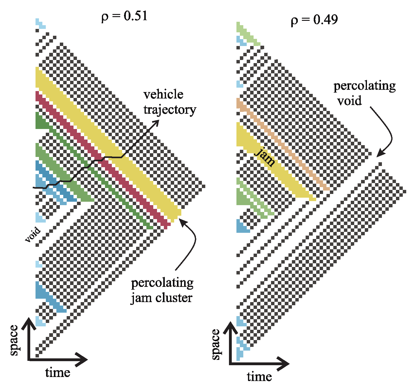
Figure 2.
Left: Coexistence curve for 77 fluids; see for the complete list. The density has been normalized to by dividing by the density of each fluid at a reduced temperature of 0.5. Inset: flow-density FDs for pedestrian traffic (light blue) along with (3) with the indicated values of (orange) estimated using nonlinear regression; 90% confidence bands shown by the dashed curves. The density has been normalized by dividing by the maximum density (in m−2) indicated in each inset. The flow has been normalized by dividing by 2 and by its 95th-percentile value. The parameter shown in each inset is needed to apply the sheer mapping to the data; see (A1)-(A2). The data come from experiments of 1-, 2- and 4-directional pedestrian traffic, as described in the following references: ref. A=[19], ref. B=[20], ref. C=[21]. Right: After applying the shear mapping to the left panel the coexistence curve is made symmetric, where the excellent fit with (3) with (black curve) is apparent. Inset: empirical flow-density macroscopic FDs for vehicular traffic for different European cities (light blue, source: [22]) along with (3) with the indicated values of (orange) estimated using nonlinear regression; 90% confidence bands shown by the dashed curves. The density has been normalized by dividing by the maximum density veh/km. The flow has been normalized by dividing by 2 and by its 95th-percentile value. The parameter shown in each inset is needed to apply the sheer mapping to the data; see (A1)-(A2).
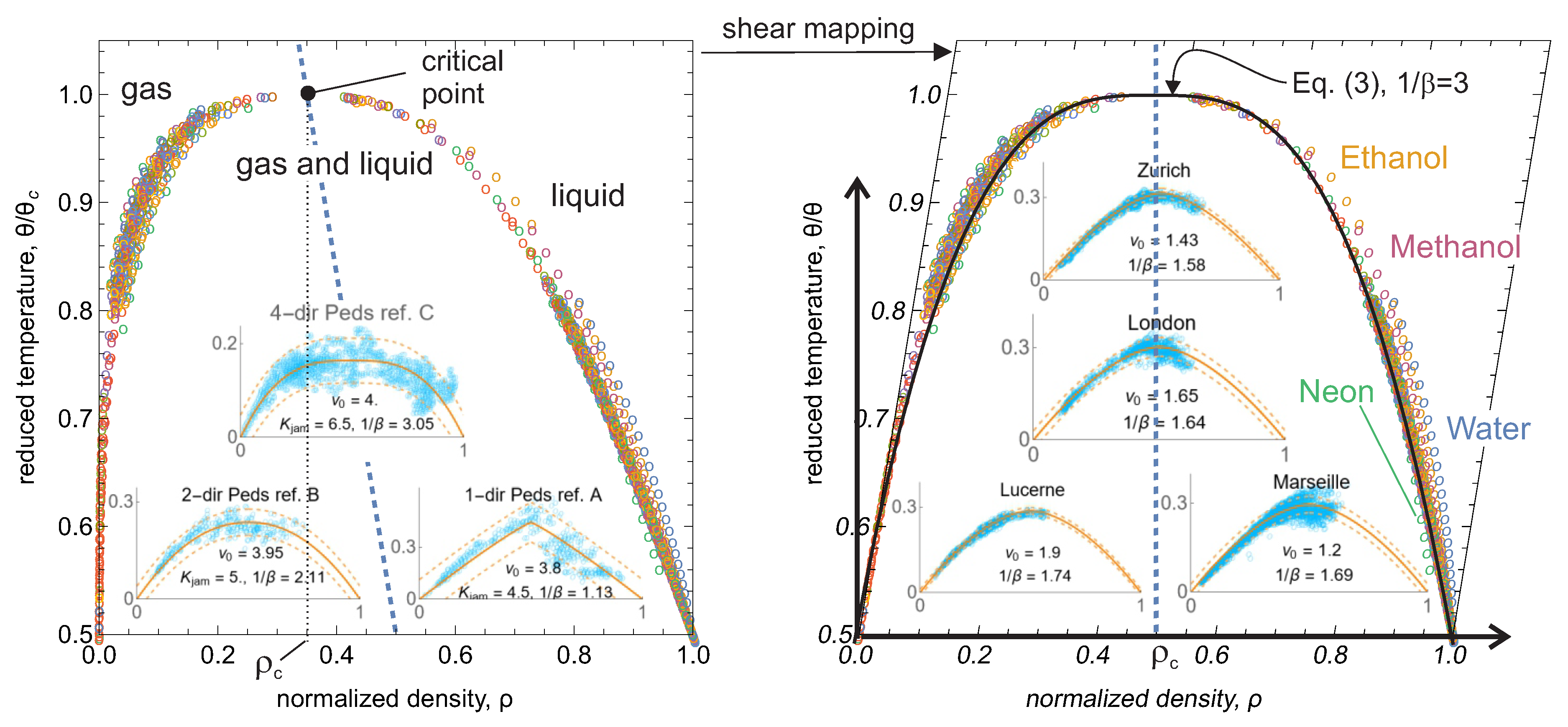
Figure 3.
The proposed FD (solid lines) along the lane-level FD assuming (4) reported in [24] (dashed lines) for different values of . Insets: The wave speed (left) and vehicle speed (right). Notice how the wave speed exhibits a discontinuity at the critical density if , but it is continuous otherwise.
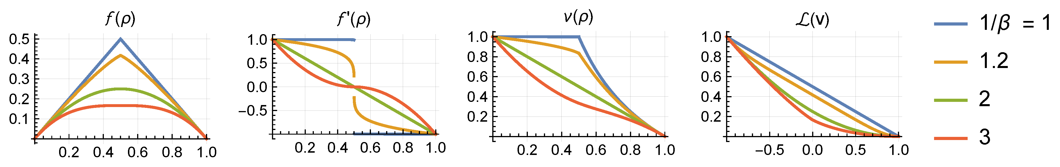
Figure 4.
The fluctuation surface per (9) produced by the NaSch model with Brownian motion initial conditions and different stopping probabilities , related to by (4). They are realizations of the (appropriately named) directed landscape process whose spatial process, the Airy process, is shown by the blue horizontal lines at times and . In the deterministic case () one can clearly see the kinematics waves propagating the fluctuations, forming self-affine fractals where the basic unit is a triangle, each containing 3 traffic states: voids (upward segments), capacity (flat segments) and jams (downward segments). The same is true in the stochastic cases shown, except that the extent of the fractal triangles is more limited due to the random interactions.
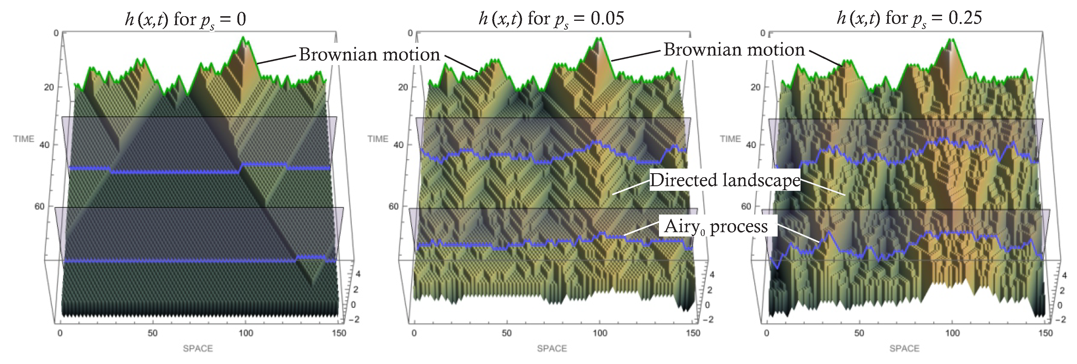
Figure 5.
Left: Log-log plot of average delay vs. road length L produced by the NaSch model for different stopping probabilities and Brownian initial conditions. The delay is computed as the total size of jam clusters, see Fig. Figure 1. The bottom inset shows a data collapse using the relationship Delay for Y-axis; same for the top inset but for flat initial conditions. Right: Log-log plot of delay versus population for the 500 largest cities in the US. Source: 2019 TTI Urban Mobility Report [61]. Inset: Log-log plot of urbanized area versus population for 130 cities in the US, 2014. Source: OECD [65]. Note: all the slopes in these plots are estimated using linear regression.
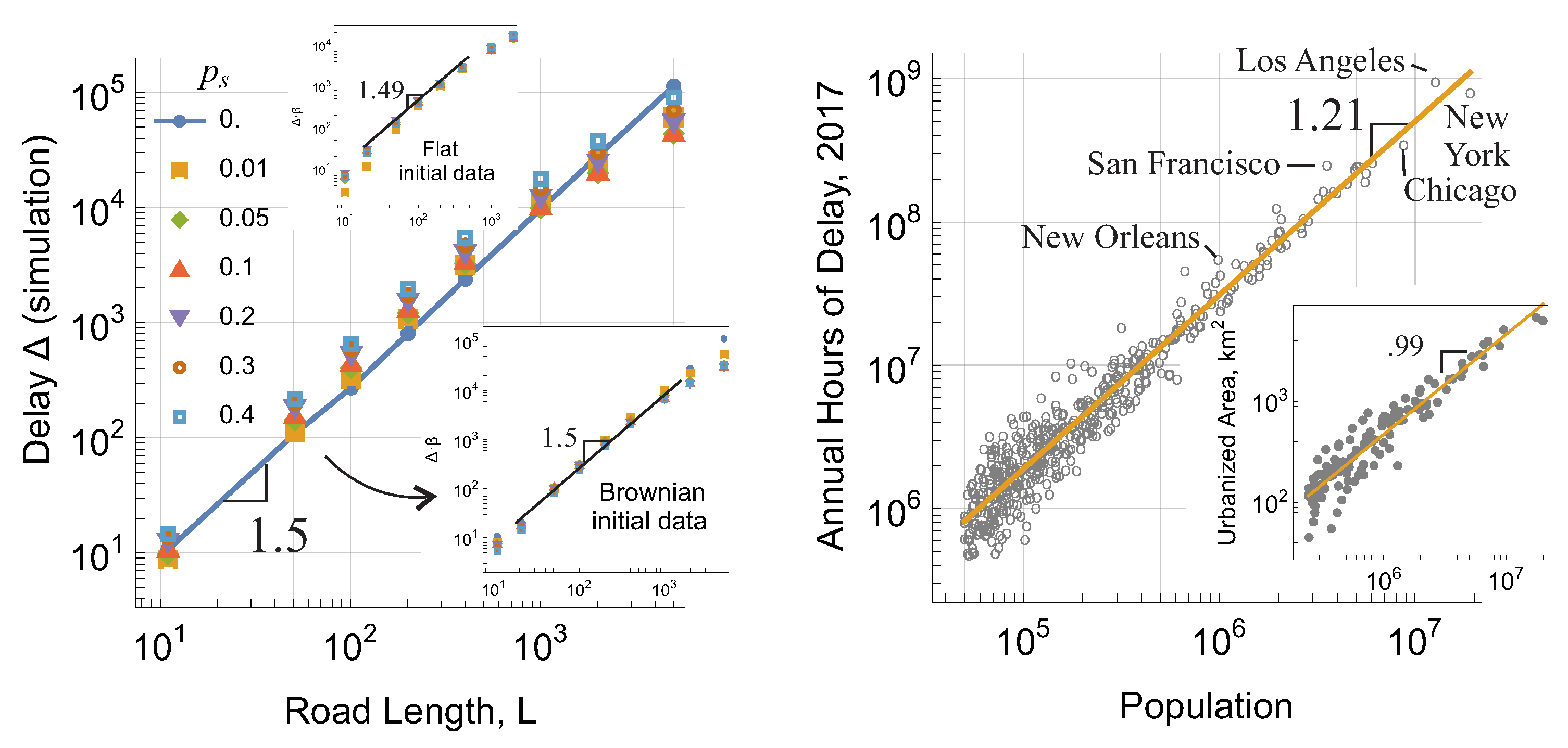

Table 1.
Fluctuation depend on the type of initial conditions.
| Brownian motion | Step | Flat | |
|---|---|---|---|
| 1-pt distribution: | |||
| Spatial process: | Airy0 | Airy1 | Airy2 |
14.1cm is the Baik–Rains distribution [50], is the Tracy-Widom GUE distribution [47], is the Tracy-Widom GUO distribution [48]. For the spatial Airy processes see [51,52,53,54,55]. For the initial conditions, suppose we divide the road into cells of length the size of a vehicle. In the Brownian motion case, each cell has equal probability of being occupied by a vehicle. In the step initial condition cells in the first half of the road segment are occupied and the rest are empty, as in a traffic signal about to turn green. Flat initial conditions represent the critical state with every other cell being occupied.
Disclaimer/Publisher’s Note: The statements, opinions and data contained in all publications are solely those of the individual author(s) and contributor(s) and not of MDPI and/or the editor(s). MDPI and/or the editor(s) disclaim responsibility for any injury to people or property resulting from any ideas, methods, instructions or products referred to in the content. |
© 2023 by the authors. Licensee MDPI, Basel, Switzerland. This article is an open access article distributed under the terms and conditions of the Creative Commons Attribution (CC BY) license (http://creativecommons.org/licenses/by/4.0/).
Copyright: This open access article is published under a Creative Commons CC BY 4.0 license, which permit the free download, distribution, and reuse, provided that the author and preprint are cited in any reuse.


