A Proof Of The Riemann Hypothesis Based On A New Expression Of The Completed Zeta Function

Weicun Zhang

doi:10.20944/preprints202108.0146.v24

Preprint

Article

This version is not peer-reviewed.

Weicun Zhang^*

This version is not peer-reviewed.

Altmetrics

Downloads

8399

Views

73068

Comments

Submitted:

20 January 2023

Posted:

20 January 2023

Read the latest preprint version here

Abstract

Based on the Hadamard product $\xi(s)= \xi(0)\prod_{\rho}(1-\frac{s}{\rho})$, a new absolute convergent expression of $\xi(s)$ is obtained by paring $\rho_i$ and $\bar{\rho}_i$, and putting all the $\rho_i$ related multiple zeros together in one factor $$\xi(s)=\xi(0)\prod_{i=1}^{\infty}\Big{(}\frac{\beta_i^2}{\alpha_i^2+\beta_i^2}+\frac{(s-\alpha_i)^2}{\alpha_i^2+\beta_i^2}\Big{)}^{d_{i}}$$ where $\xi(0)=\frac{1}{2}$, $\rho_i=\alpha_i+j\beta_i$ and $\bar{\rho}_i=\alpha_i-j\beta_i$ are the complex conjugate zeros of $\xi(s)$, $0<\alpha_i<1$ and $\beta_i\neq 0$ are real numbers, $d_i\geq 1$ are the real multiplicities of $\rho_i$, $\beta_i$ are in order of increasing $|\beta_i|$. Then, by the functional equation $\xi(s)=\xi(1-s)$, we have $$\xi(0)\prod_{i=1}^{\infty}\Big{(}\frac{\beta_i^2}{\alpha_i^2+\beta_i^2}+\frac{(s-\alpha_i)^2}{\alpha_i^2+\beta_i^2}\Big{)}^{d_{i}} =\xi(0)\prod_{i=1}^{\infty}\Big{(}\frac{\beta_i^2}{\alpha_i^2+\beta_i^2}+\frac{(1-s-\alpha_i)^2}{\alpha_i^2+\beta_i^2}\Big{)}^{d_{i}}$$ i.e., $$\prod_{i=1}^{\infty}\Big{(}1+\frac{(s-\alpha_i)^2}{\beta_i^2}\Big{)}^{d_{i}}=\prod_{i=1}^{\infty}\Big{(}1+\frac{(1-s-\alpha_i)^2}{\beta_i^2}\Big{)}^{d_{i}}$$ which, by Lemma 3, is equivalent to $$\begin{cases}&\alpha_i=\frac{1}{2}, i =1,2,3, \cdots, \infty\\ & \beta_1<\beta_2<\beta_3<\cdots\\ \end{cases}$$ Thus, we conclude that the Riemann Hypothesis is true.

Keywords:

Subject:

Computer Science and Mathematics - Algebra and Number Theory

This preprints belongs to the Collection

Preprints.org 2023 Most Popular Preprints Award Winner Collection

1. Introduction

It has been almost 163 years since the Riemann Hypothesis (RH) was proposed in

1859^{[1]}

. Many efforts and achievements have been made towards proving this celebrated hypothesis, but it is still an open

{problem}^{[2 - 3]}

The Riemann zeta function is the function of the complex variable s, defined in the half-plane

ℜ (s) > 1

by the absolutely convergent

{series}^{[2]}

ζ (s) = \sum_{n = 1}^{\infty} \frac{1}{n^{s}}, ℜ (s) > 1

(1)

The connection between the Riemann zeta function and prime numbers can be established through the well-known Euler product, i.e.

ζ (s) = \sum_{n = 1}^{\infty} \frac{1}{n^{s}} = \prod_{p} {(1 - p^{- s})}^{- 1}, ℜ (s) > 1

(2)

where p runs over the prime numbers.

Riemann showed how to extend zeta function to the whole complex plane

C

by analytic continuation

ζ (s) = \frac{π^{s / 2}}{Γ (s / 2)} {\frac{1}{s (s - 1)} + \int_{1}^{\infty} (x^{\frac{s}{2} - 1} + x^{- \frac{s}{2} - \frac{1}{2}}) \cdot (\frac{θ (x) - 1}{2}) d x}

(3)

where

θ (x) = \sum_{- \infty}^{\infty} e^{- n^{2} π x}

being the Jaccobi theta function,

Γ

being the Gamma function in the following Weierstrass expression (Meanwhile, there are also Gauss expression, Euler expression, and integral expression of the Gamma function.)

\frac{1}{Γ (s)} = s \cdot e^{γ s} \prod_{n = 1}^{\infty} (1 + \frac{s}{n}) e^{- s / n}

(4)

where

γ

is the Euler-Mascheroni constant.

As shown by Riemann,

ζ (s)

extends to

C

as a meromorphic function with only a simple pole at

s = 1

, with residue 1, and satisfies the following functional equation

π^{- \frac{s}{2}} Γ (\frac{s}{2}) ζ (s) = π^{- \frac{1 - s}{2}} Γ (\frac{1 - s}{2}) ζ (1 - s)

(5)

The Riemann zeta function

ζ (s)

has zeros at the negative even integers:

- 2

- 4

- 6

- 8

, ⋯ and one refers to them as the trivial zeros. The other zeros of

ζ (s)

are the complex numbers, i.e., non-trivial

{zeros}^{[2]}

In 1896,

{Hadamard}^{[4]}

and

{Poussin}^{[5]}

independently proved that no zeros could lie on the line

ℜ (s) = 1

. Together with the functional equation and the fact that there are no zeros with real part greater than 1, this showed that all non-trivial zeros must lie in the interior of the critical strip

0 < ℜ (s) < 1

. This was a key step in their first proofs of the famous Prime Number Theorem.

Later on, Hardy (1914

)^{[6]}

, Hardy and Littlewood (1921

)^{[7]}

showed that there are infinitely many zeros on the critical line

ℜ (s) = \frac{1}{2}

, which was an astonishing result at that time.

As a summary, we have the following results on the properties of the non-trivial zeros of

ζ (s)

^[4−9].

Lemma 1:

Non-trivial zeroes of

ζ (s)

, noted as

ρ = α + j β

, have the following properties

1): The number of non-trivial zeroes is infinity;
2): $β \neq 0$ ;
3): $0 < α < 1$ ;
4): $ρ, \bar{ρ}, 1 - \bar{ρ}, 1 - ρ$ are all non-trivial zeroes.

As further study, a completed zeta function

ξ (s)

is defined as

ξ (s) = \frac{1}{2} s (s - 1) π^{- \frac{s}{2}} Γ (\frac{s}{2}) ζ (s)

(6)

It is well-known that

ξ (s)

is an entire function of order 1. This implies

ξ (s)

is analytic, and can be expressed as infinite polynomial, in the whole complex plane

C

In addition, replacing s with

1 - s

in Eq.(6), and combining Eq.(5), we have the following functional equation

ξ (s) = ξ (1 - s)

(7)

Considering the definition of

ξ (s)

, and recalling Eq.(4), the trivial zeros of

ζ (s)

are canceled by the poles of

Γ (\frac{s}{2})

. The zero of

s - 1

and the pole of

ζ (s)

cancel; the zero

s = 0

and the pole of

Γ (\frac{s}{2})

{cancel}^{[9 - 10]}

. Thus, all the zeros of

ξ (s)

are exactly the nontrivial zeros of

ζ (s)

. Then we have the following Lemma 2.

Lemma 2:

The zeros of

ξ (s)

coincide with the non-trivial zeros of

ζ (s)

According to Lemma 2, the following two statements for the RH are equivalent.

Statement 1 of the RH:

All the non-trivial zeros of

ζ (s)

have real part equal to

\frac{1}{2}

Statement 2 of the RH:

All the zeros of

ξ (s)

have real part equal to

\frac{1}{2}

To prove the RH, a natural thinking is to estimate the numbers of non-trivial zeros of

ζ (s)

inside or outside some areas according to Argument Principle. Along this train of thought, there are many research works. Let

N (T)

denote the number of zeros of

ζ (s)

inside the rectangle:

0 < α < 1, 0 < β \leq T

, and let

N_{0} (T)

denote the number of zeros of

ζ (s)

on the line

α = \frac{1}{2}, 0 < β \leq T

. Selberg proved that there exist positive constants c and

T_{0}

, such that

N_{0} (T) > c N (T), (T > T_{0})^{[11]}

, later on, Levinson proved that

c \geq \frac{1}{3}

^[12], Lou and Yao proved that

c \geq {0.3484}^{[13]}

, Conrey proved that

c \geq {\frac{2}{5}}^{[14]}

, Bui, Conrey and Young proved that

c \geq {0.41}^{[15]}

, Feng proved that

c \geq {0.4128}^{[16]}

On the other hand, many zeros have been calculated by hand or by computer programs. Among others, Riemann found the first three non-trivial

{zeros}^{[17]}

. Gram found the first 15 zeros based on Euler-Maclaurin

{summation}^{[18]}

. Titchmarsh calculated the 138^th to 195^th zeros using the Riemann-Siegel

{formula}^{[19 - 20]}

. Here are the first three (pairs of) zeros:

\frac{1}{2} \pm j 14.1347251; \frac{1}{2} \pm j 21.0220396; \frac{1}{2} \pm j 25.0108575

The idea of this paper is originated from Euler’s work on proving the following famous equality

1 + \frac{1}{2^{2}} + \frac{1}{3^{2}} + \frac{1}{4^{2}} + \frac{1}{5^{2}} + \dots = \frac{π^{2}}{6}

(8)

This interesting result is deduced by comparing the like terms of two types of infinite expressions, i.e., infinite polynomial and infinite product, as shown in the following

\begin{matrix} \frac{sin x}{x} & = 1 - \frac{x^{2}}{3!} + \frac{x^{4}}{5!} - \frac{x^{6}}{7!} + \dots \\ = (1 - \frac{x^{2}}{π^{2}}) (1 - \frac{x^{2}}{4 π^{2}}) (1 - \frac{x^{2}}{9 π^{2}}) \dots \end{matrix}

(9)

Then it is conjectured that

ξ (s)

should be factored into

(1 + \frac{{(s - α_{i})}^{2}}{β_{i}^{2}})

or something like that, which was verified by paring

ρ_{i}

and

{\bar{ρ}}_{i}

in the Hadamard product of

ξ (s)

to obtain

(1 - \frac{s}{ρ_{i}}) (1 - \frac{s}{{\bar{ρ}}_{i}}) = \frac{β_{i}^{2}}{α_{i}^{2} + β_{i}^{2}} (1 + \frac{{(s - α_{i})}^{2}}{β_{i}^{2}})

The Hadamard product of

ξ (s)

as shown in Eq.(10) was first proposed by Riemann, however, it was

{Hadamard}^{[21]}

who showed the validity of this infinite product expansion.

ξ (s) = ξ (0) \prod_{ρ} (1 - \frac{s}{ρ})

(10)

where

ξ (0) = \frac{1}{2}

ρ

runs over all the non-trivial zeros of the Riemann zeta function

ζ (s)

, or in another word,

ρ

runs over all the zeros of the completed zeta function

ξ (s)

To ensure the absolute convergence of the infinite product expansion,

ρ

and

1 - ρ

are paired. Later in Section 3, we will show that

ρ

and

\bar{ρ}

can also be paired to ensure the absolute convergence of the infinite product expansion.

2. Lemmas

In this section, we first explain the concepts of multiple zeros of

ξ (s)

with their real multiplicities. And then we give three lemmas to support the proof of the RH, in which Lemma 3 is the key lemma.

Multiple zeros of

ξ (s)

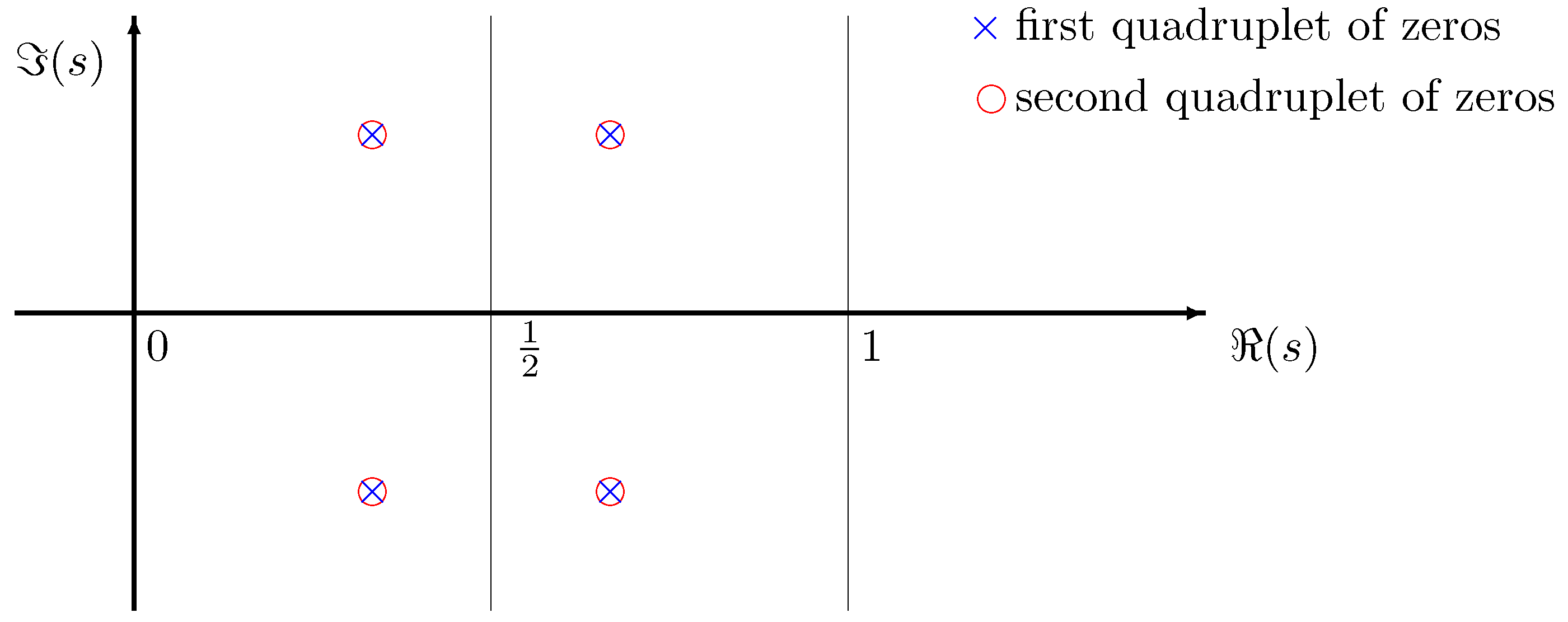
As shown in Figure 1, the multiple zeros of

ξ (s)

are defined in terms of the quadruplet, i.e.,

ρ, \bar{ρ}, 1 - ρ, 1 - \bar{ρ}

It should be noticed that the multiple zeros with their real multiplicities of

ξ (s)

are objective existence, but the expression of the corresponding factors of

ξ (s)

are optional to some extent. For example, the multiple zeros as shown in Figure 1 have two different expressions as factors of

ξ (s)

and

ξ (1 - s)

, respectively, i.e.,

[(1 + \frac{{(s - α_{1})}^{2}}{β_{1}^{2}})^{2}, (1 + \frac{{(1 - s - α_{1})}^{2}}{β_{1}^{2}})^{2}]

, or

[(1 + \frac{{(s - α_{1})}^{2}}{β_{1}^{2}}) (1 + \frac{{(s - α_{2})}^{2}}{β_{2}^{2}}), (1 + \frac{{(1 - s - α_{1})}^{2}}{β_{1}^{2}}) (1 + \frac{{(1 - s - α_{2})}^{2}}{β_{2}^{2}}), α_{1} + α_{2} = 1, β_{1} = β_{2}]

To exclude the latter expression, we stipulate that the multiple zero

ρ_{i}

related factor of

ξ (s)

takes the form of

(1 + \frac{{(s - α_{i})}^{2}}{β_{i}^{2}})^{d_{i}}

, where

d_{i} \geq 1

is the real multiplicity of

ρ_{i}

Lemma 3:

Given two infinite products

f (s) = \prod_{i = 1}^{\infty} (1 + \frac{{(s - α_{i})}^{2}}{β_{i}^{2}})^{d_{i}}

(11)

and

f (1 - s) = \prod_{i = 1}^{\infty} (1 + \frac{{(1 - s - α_{i})}^{2}}{β_{i}^{2}})^{d_{i}}

(12)

where s is a complex variable,

ρ_{i} = α_{i} + j β_{i}

and

{\bar{ρ}}_{i} = α_{i} - j β_{i}

are the complex conjugate zeros of

ξ (s)

0 < α_{i} < 1

and

β_{i} \neq 0

are real numbers,

d_{i} \geq 1

are the real multiplicities of

ρ_{i}

, i are natural numbers from 1 to infinity,

β_{i}

are in order of increasing

| β_{i} |

, i.e.,

| β_{1} | \leq | β_{2} | \leq | β_{3} | \leq \dots

Then we have

f (s) = f (1 - s) \Leftrightarrow \{\begin{matrix} α_{i} = \frac{1}{2}, i = 1, 2, 3, \dots, \infty \\ β_{1} < β_{2} < β_{3} < \dots \end{matrix}

(13)

where

" \Leftrightarrow "

is the equivalent sign.

Proof :

First of all, we have the following fact:

\begin{matrix} (1 + \frac{{(s - α)}^{2}}{β^{2}})^{d} = (1 + \frac{{(1 - s - α)}^{2}}{β^{2}})^{d} \\ \Leftrightarrow {(s - α)}^{2} = {(1 - s - α)}^{2} \Leftrightarrow α = \frac{1}{2} \end{matrix}

(14)

where

d \geq 1

is a natural number,

α \neq 0

and

β \neq 0

are real numbers.

Next, the proof is based on Transfinite Induction. Let

P (n)

be:

\begin{matrix} \prod_{i = 1}^{n} (1 + \frac{{(s - α_{i})}^{2}}{β_{i}^{2}})^{d_{i}} = \prod_{i = 1}^{n} (1 + \frac{{(1 - s - α_{i})}^{2}}{β_{i}^{2}})^{d_{i}} \\ \Leftrightarrow \\ \{\begin{matrix} (1 + \frac{{(s - α_{1})}^{2}}{β_{1}^{2}})^{d_{1}} = (1 + \frac{{(1 - s - α_{1})}^{2}}{β_{1}^{2}})^{d_{1}} \\ \dots \\ (1 + \frac{{(s - α_{n})}^{2}}{β_{n}^{2}})^{d_{n}} = (1 + \frac{{(1 - s - α_{n})}^{2}}{β_{n}^{2}})^{d_{n}} \\ β_{1} < β_{2} < β_{3} < \dots < β_{n} \end{matrix} \\ \Leftrightarrow \\ \{\begin{matrix} α_{i} = \frac{1}{2}, i = 1 \dots n \\ β_{1} < β_{2} < β_{3} < \dots < β_{n} \end{matrix} \end{matrix}

(15)

According to Eq.(14),

P (1)

is an obvious fact as the Base Case, i.e.,

\begin{matrix} \prod_{i = 1}^{1} (1 + \frac{{(s - α_{i})}^{2}}{β_{i}^{2}})^{d_{i}} = \prod_{i = 1}^{1} (1 + \frac{{(1 - s - α_{i})}^{2}}{β_{i}^{2}})^{d_{i}} \\ \Leftrightarrow (1 + \frac{{(s - α_{1})}^{2}}{β_{1}^{2}})^{d_{1}} = (1 + \frac{{(1 - s - α_{1})}^{2}}{β_{1}^{2}})^{d_{1}} \\ \Leftrightarrow α_{1} = \frac{1}{2} \end{matrix}

(16)

To be more convincing, let’s further check

P (2)

, i.e.,

\begin{matrix} \prod_{i = 1}^{2} (1 + \frac{{(s - α_{i})}^{2}}{β_{i}^{2}})^{d_{i}} = \prod_{i = 1}^{2} (1 + \frac{{(1 - s - α_{i})}^{2}}{β_{i}^{2}})^{d_{i}} \\ \Leftrightarrow \\ \{\begin{matrix} (1 + \frac{{(s - α_{1})}^{2}}{β_{1}^{2}})^{d_{1}} = (1 + \frac{{(1 - s - α_{1})}^{2}}{β_{1}^{2}})^{d_{1}} \\ (1 + \frac{{(s - α_{2})}^{2}}{β_{2}^{2}})^{d_{2}} = (1 + \frac{{(1 - s - α_{2})}^{2}}{β_{2}^{2}})^{d_{2}} \\ β_{1} < β_{2} \end{matrix} \\ \Leftrightarrow \\ \{\begin{matrix} α_{1} = α_{2} = \frac{1}{2} \\ β_{1} < β_{2} \end{matrix} \end{matrix}

(17)

which is also an obvious fact according to Lemma 5.

As the Successor Case, we need to prove

P (n) \Rightarrow P (n + 1)

Actually, we have

\begin{matrix} \prod_{i = 1}^{n + 1} (1 + \frac{{(s - α_{i})}^{2}}{β_{i}^{2}})^{d_{i}} = \prod_{i = 1}^{n + 1} (1 + \frac{{(1 - s - α_{i})}^{2}}{β_{i}^{2}})^{d_{i}} \\ \Leftrightarrow \\ \prod_{i = 1}^{n} (1 + \frac{{(s - α_{i})}^{2}}{β_{i}^{2}})^{d_{i}} (1 + \frac{{(s - α_{n + 1})}^{2}}{β_{n + 1}^{2}})^{d_{n + 1}} = \prod_{i = 1}^{n} (1 + \frac{{(1 - s - α_{i})}^{2}}{β_{i}^{2}})^{d_{i}} (1 + \frac{{(1 - s - α_{n + 1})}^{2}}{β_{n + 1}^{2}})^{d_{n + 1}} \\ \Leftrightarrow (by Lemma 5) \\ \{\begin{matrix} \prod_{i = 1}^{n} (1 + \frac{{(s - α_{i})}^{2}}{β_{i}^{2}})^{d_{i}} = \prod_{i = 1}^{n} (1 + \frac{{(1 - s - α_{i})}^{2}}{β_{i}^{2}})^{d_{i}} \\ (1 + \frac{{(s - α_{n + 1})}^{2}}{β_{n + 1}^{2}})^{d_{n + 1}} = (1 + \frac{{(1 - s - α_{n + 1})}^{2}}{β_{n + 1}^{2}})^{d_{n + 1}} \\ β_{1} < β_{2} < β_{3} < \dots < β_{n} < β_{n + 1} \end{matrix} \\ \Leftrightarrow (by Eq . (15)) \\ \{\begin{matrix} (1 + \frac{{(s - α_{1})}^{2}}{β_{1}^{2}})^{d_{1}} = (1 + \frac{{(1 - s - α_{1})}^{2}}{β_{1}^{2}})^{d_{1}} \\ \dots \\ (1 + \frac{{(s - α_{n + 1})}^{2}}{β_{n + 1}^{2}})^{d_{n + 1}} = (1 + \frac{{(1 - s - α_{n + 1})}^{2}}{β_{n + 1}^{2}})^{d_{n + 1}} \\ β_{1} < β_{2} < β_{3} < \dots < β_{n} < β_{n + 1} \end{matrix} \\ \Leftrightarrow (by Eq . (14)) \\ \{\begin{matrix} α_{i} = \frac{1}{2}, i = 1, 2, 3, \dots, n, n + 1 \\ β_{1} < β_{2} < β_{3} < \dots < β_{n} < β_{n + 1} \end{matrix} \end{matrix}

(18)

Thus the Successor Case is true, i.e.,

P (n) \Rightarrow P (n + 1)

Next, we prove that

P (\infty)

holds by considering well-ordered ordinal set A indexing the family of statements

P (γ : γ \in A)

A = N ⋃ {ω}

with the ordering that

n < ω

for all natural numbers n,

ω

is the first limit ordinal.

It is well-known that

ω = ⋃ {γ : γ < ω}

To prove that

P (\infty)

holds, it suffices to prove the Limit Case, i.e.,

P (γ < ω) \Rightarrow P (ω)

Actually, we have

\begin{matrix} \prod_{i = 1}^{ω} (1 + \frac{{(s - α_{i})}^{2}}{β_{i}^{2}})^{d_{i}} = \prod_{i = 1}^{ω} (1 + \frac{{(1 - s - α_{i})}^{2}}{β_{i}^{2}})^{d_{i}} \\ \Leftrightarrow \\ \prod_{i = 1}^{γ < ω} (1 + \frac{{(s - α_{i})}^{2}}{β_{i}^{2}})^{d_{i}} (1 + \frac{{(s - α_{ω})}^{2}}{β_{ω}^{2}})^{d_{ω}} = \prod_{i = 1}^{γ < ω} (1 + \frac{{(1 - s - α_{i})}^{2}}{β_{i}^{2}})^{d_{i}} (1 + \frac{{(1 - s - α_{ω})}^{2}}{β_{ω}^{2}})^{d_{ω}} \\ \Leftrightarrow (by Lemma 5) \\ \{\begin{matrix} \prod_{i = 1}^{γ < ω} (1 + \frac{{(s - α_{i})}^{2}}{β_{i}^{2}})^{d_{i}} = \prod_{i = 1}^{γ < ω} (1 + \frac{{(1 - s - α_{i})}^{2}}{β_{i}^{2}})^{d_{i}} \\ (1 + \frac{{(s - α_{ω})}^{2}}{β_{ω}^{2}})^{d_{ω}} = (1 + \frac{{(1 - s - α_{ω})}^{2}}{β_{ω}^{2}})^{d_{ω}} \\ β_{1} < β_{2} < β_{3} < \dots < β_{ω} \end{matrix} \\ \Leftrightarrow (by P (γ < ω)) \\ \{\begin{matrix} (1 + \frac{{(s - α_{1})}^{2}}{β_{1}^{2}})^{d_{1}} = (1 + \frac{{(1 - s - α_{1})}^{2}}{β_{1}^{2}})^{d_{1}} \\ \dots \\ (1 + \frac{{(s - α_{ω})}^{2}}{β_{ω}^{2}})^{d_{ω}} = (1 + \frac{{(1 - s - α_{ω})}^{2}}{β_{ω}^{2}})^{d_{ω}} \\ β_{1} < β_{2} < β_{3} < \dots < β_{ω} \end{matrix} \\ \Leftrightarrow (by Eq . (14)) \\ \{\begin{matrix} α_{i} = \frac{1}{2}, i = 1, 2, 3, \dots, ω \\ β_{1} < β_{2} < β_{3} < \dots < β_{ω} \end{matrix} \end{matrix}

(19)

Thus the Limit Case is true, i.e.,

P (γ < ω) \Rightarrow P (ω)

Hence we conclude by Transfinite Induction that

P (\infty)

holds, i.e.,

\begin{matrix} \prod_{i = 1}^{\infty} (1 + \frac{{(s - α_{i})}^{2}}{β_{i}^{2}})^{d_{i}} = \prod_{i = 1}^{\infty} (1 + \frac{{(1 - s - α_{i})}^{2}}{β_{i}^{2}})^{d_{i}} \\ \Leftrightarrow \\ \{\begin{matrix} (1 + \frac{{(s - α_{1})}^{2}}{β_{1}^{2}})^{d_{1}} = (1 + \frac{{(1 - s - α_{1})}^{2}}{β_{1}^{2}})^{d_{1}} \\ \dots \\ (1 + \frac{{(s - α_{i})}^{2}}{β_{i}^{2}})^{d_{i}} = (1 + \frac{{(1 - s - α_{i})}^{2}}{β_{i}^{2}})^{d_{i}} \\ \dots \\ β_{1} < β_{2} < β_{3} < \dots \end{matrix} \\ \Leftrightarrow \\ \{\begin{matrix} α_{i} = \frac{1}{2}, i = 1 \dots \infty \\ β_{1} < β_{2} < β_{3} < \dots \end{matrix} \end{matrix}

(20)

i.e.,

f (s) = f (1 - s) \Leftrightarrow \{\begin{matrix} α_{i} = \frac{1}{2}, i = 1, 2, 3, \dots, \infty \\ β_{1} < β_{2} < β_{3} < \dots \end{matrix}

(21)

That completes the proof of Lemma 3.

Lemma 4:

Given

(1 + \frac{{(s - α_{1})}^{2}}{β_{1}^{2}}) (1 + \frac{{(s - α_{2})}^{2}}{β_{2}^{2}}) = (1 + \frac{{(1 - s - α_{1})}^{2}}{β_{1}^{2}}) (1 + \frac{{(1 - s - α_{2})}^{2}}{β_{2}^{2}})

(22)

where s is a complex variable,

0 < α_{i} < 1

and

β_{i} \neq 0

are real numbers,

| β_{1} | \leq | β_{2} |

Then we have

\begin{matrix} (1 + \frac{{(s - α_{1})}^{2}}{β_{1}^{2}}) (1 + \frac{{(s - α_{2})}^{2}}{β_{2}^{2}}) = (1 + \frac{{(1 - s - α_{1})}^{2}}{β_{1}^{2}}) (1 + \frac{{(1 - s - α_{2})}^{2}}{β_{2}^{2}}) \\ \Leftrightarrow \\ \{\begin{matrix} α_{1} = α_{2} = \frac{1}{2}, & β_{1} \neq β_{2} \\ α_{1} + α_{2} = 1, & β_{1} = β_{2} \end{matrix} \\ \Leftrightarrow \\ \{\begin{matrix} (1 + \frac{{(s - α_{1})}^{2}}{β_{1}^{2}}) = (1 + \frac{{(1 - s - α_{1})}^{2}}{β_{1}^{2}}), (1 + \frac{{(s - α_{2})}^{2}}{β_{2}^{2}}) = (1 + \frac{{(1 - s - α_{2})}^{2}}{β_{2}^{2}}), & β_{1} \neq β_{2} \\ (1 + \frac{{(s - α_{1})}^{2}}{β_{1}^{2}}) = (1 + \frac{{(1 - s - α_{2})}^{2}}{β_{2}^{2}}), (1 + \frac{{(s - α_{2})}^{2}}{β_{2}^{2}}) = (1 + \frac{{(1 - s - α_{1})}^{2}}{β_{1}^{2}}), & β_{1} = β_{2} \end{matrix} \end{matrix}

(23)

Proof :

Expanding both sides of Eq.(22), and comparing the coefficients of like terms, we obtain (details are omitted to save space)

\begin{matrix} (1 + \frac{{(s - α_{1})}^{2}}{β_{1}^{2}}) (1 + \frac{{(s - α_{2})}^{2}}{β_{2}^{2}}) = (1 + \frac{{(1 - s - α_{1})}^{2}}{β_{1}^{2}}) (1 + \frac{{(1 - s - α_{2})}^{2}}{β_{2}^{2}}) \\ \Rightarrow \\ \{\begin{matrix} α_{1} = α_{2} = \frac{1}{2}, & β_{1} \neq β_{2} \\ α_{1} + α_{2} = 1, & β_{1} = β_{2} \end{matrix} \end{matrix}

(24)

The inverse inference of Eq.(24) is also an obvious fact. i.e.,

\begin{matrix} \{\begin{matrix} α_{1} = α_{2} = \frac{1}{2}, & β_{1} \neq β_{2} \\ α_{1} + α_{2} = 1, & β_{1} = β_{2} \end{matrix} \\ \Rightarrow \\ (1 + \frac{{(s - α_{1})}^{2}}{β_{1}^{2}}) (1 + \frac{{(s - α_{2})}^{2}}{β_{2}^{2}}) = (1 + \frac{{(1 - s - α_{1})}^{2}}{β_{1}^{2}}) (1 + \frac{{(1 - s - α_{2})}^{2}}{β_{2}^{2}}) \end{matrix}

Then we have

\begin{matrix} (1 + \frac{{(s - α_{1})}^{2}}{β_{1}^{2}}) (1 + \frac{{(s - α_{2})}^{2}}{β_{2}^{2}}) = (1 + \frac{{(1 - s - α_{1})}^{2}}{β_{1}^{2}}) (1 + \frac{{(1 - s - α_{2})}^{2}}{β_{2}^{2}}) \\ \Leftrightarrow \\ \{\begin{matrix} α_{1} = α_{2} = \frac{1}{2}, & β_{1} \neq β_{2} \\ α_{1} + α_{2} = 1, & β_{1} = β_{2} \end{matrix} \end{matrix}

(25)

Further, according to Eq.(14), i.e.,

(1 + \frac{{(s - α)}^{2}}{β^{2}})^{d} = (1 + \frac{{(1 - s - α)}^{2}}{β^{2}})^{d} \Leftrightarrow α = \frac{1}{2}

and the following similar facts

(1 + \frac{{(s - α_{1})}^{2}}{β_{1}^{2}}) = (1 + \frac{{(1 - s - α_{2})}^{2}}{β_{2}^{2}}) \Leftrightarrow α_{1} + α_{2} = 1, β_{1} = β_{2}

(1 + \frac{{(s - α_{2})}^{2}}{β_{2}^{2}}) = (1 + \frac{{(1 - s - α_{1})}^{2}}{β_{1}^{2}}) \Leftrightarrow α_{1} + α_{2} = 1, β_{1} = β_{2}

we have

\begin{matrix} (1 + \frac{{(s - α_{1})}^{2}}{β_{1}^{2}}) (1 + \frac{{(s - α_{2})}^{2}}{β_{2}^{2}}) = (1 + \frac{{(1 - s - α_{1})}^{2}}{β_{1}^{2}}) (1 + \frac{{(1 - s - α_{2})}^{2}}{β_{2}^{2}}) \\ \Leftrightarrow \\ \{\begin{matrix} α_{1} = α_{2} = \frac{1}{2}, & β_{1} \neq β_{2} \\ α_{1} + α_{2} = 1, & β_{1} = β_{2} \end{matrix} \\ \Leftrightarrow \\ \{\begin{matrix} (1 + \frac{{(s - α_{1})}^{2}}{β_{1}^{2}}) = (1 + \frac{{(1 - s - α_{1})}^{2}}{β_{1}^{2}}), (1 + \frac{{(s - α_{2})}^{2}}{β_{2}^{2}}) = (1 + \frac{{(1 - s - α_{2})}^{2}}{β_{2}^{2}}), & β_{1} \neq β_{2} \\ (1 + \frac{{(s - α_{1})}^{2}}{β_{1}^{2}}) = (1 + \frac{{(1 - s - α_{2})}^{2}}{β_{2}^{2}}), (1 + \frac{{(s - α_{2})}^{2}}{β_{2}^{2}}) = (1 + \frac{{(1 - s - α_{1})}^{2}}{β_{1}^{2}}), & β_{1} = β_{2} \end{matrix} \end{matrix}

(26)

That completes the proof of Lemma 4.

Lemma 5:

Given

(1 + \frac{{(s - α_{1})}^{2}}{β_{1}^{2}})^{d_{1}} (1 + \frac{{(s - α_{2})}^{2}}{β_{2}^{2}})^{d_{2}} = (1 + \frac{{(1 - s - α_{1})}^{2}}{β_{1}^{2}})^{d_{1}} (1 + \frac{{(1 - s - α_{2})}^{2}}{β_{2}^{2}})^{d_{2}}

(27)

where s is a complex variable,

0 < α_{1} < 1, 0 < α_{2} < 1

and

β_{1} \neq 0, β_{2} \neq 0

are real numbers,

d_{1} \geq 1, d_{2} \geq 1

are natural numbers, denoting the real multiplicities of

ρ_{1} = α_{1} + j β_{1}

and

ρ_{2} = α_{2} + j β_{2}

, respectively,

| β_{1} | \leq | β_{2} |

Then we have

\begin{matrix} (1 + \frac{{(s - α_{1})}^{2}}{β_{1}^{2}})^{d_{1}} (1 + \frac{{(s - α_{2})}^{2}}{β_{2}^{2}})^{d_{2}} = (1 + \frac{{(1 - s - α_{1})}^{2}}{β_{1}^{2}})^{d_{1}} (1 + \frac{{(1 - s - α_{2})}^{2}}{β_{2}^{2}})^{d_{2}} \\ \Leftrightarrow \\ \{\begin{matrix} α_{1} = α_{2} = \frac{1}{2} \\ β_{1} < β_{2} \end{matrix} \\ \Leftrightarrow \\ \{\begin{matrix} (1 + \frac{{(s - α_{1})}^{2}}{β_{1}^{2}})^{d_{1}} = (1 + \frac{{(1 - s - α_{1})}^{2}}{β_{1}^{2}})^{d_{1}} \\ (1 + \frac{{(s - α_{2})}^{2}}{β_{2}^{2}})^{d_{2}} = (1 + \frac{{(1 - s - α_{2})}^{2}}{β_{2}^{2}})^{d_{2}} \\ β_{1} < β_{2} \end{matrix} \end{matrix}

(28)

Proof :

Based on Lemma 4, and considering additional possibilities that

(1 + \frac{{(s - α_{1})}^{2}}{β_{1}^{2}})^{d_{1}} ∣ (1 + \frac{{(1 - s - α_{2})}^{2}}{β_{2}^{2}})^{d_{2}}

(1 + \frac{{(1 - s - α_{1})}^{2}}{β_{1}^{2}})^{d_{1}} ∣ (1 + \frac{{(s - α_{2})}^{2}}{β_{2}^{2}})^{d_{2}}

(where "∣" is the divisible sign), or vice versa, we have

\begin{matrix} (1 + \frac{{(s - α_{1})}^{2}}{β_{1}^{2}})^{d_{1}} (1 + \frac{{(s - α_{2})}^{2}}{β_{2}^{2}})^{d_{2}} = (1 + \frac{{(1 - s - α_{1})}^{2}}{β_{1}^{2}})^{d_{1}} (1 + \frac{{(1 - s - α_{2})}^{2}}{β_{2}^{2}})^{d_{2}} \\ \Leftrightarrow \\ \{\begin{matrix} (1 + \frac{{(s - α_{1})}^{2}}{β_{1}^{2}})^{d_{1}} = (1 + \frac{{(1 - s - α_{1})}^{2}}{β_{1}^{2}})^{d_{1}}, (1 + \frac{{(s - α_{2})}^{2}}{β_{2}^{2}})^{d_{2}} = (1 + \frac{{(1 - s - α_{2})}^{2}}{β_{2}^{2}})^{d_{2}}, & β_{1} < β_{2} \\ \{\begin{matrix} (1 + \frac{{(s - α_{1})}^{2}}{β_{1}^{2}})^{d_{1}} ∣ (1 + \frac{{(1 - s - α_{2})}^{2}}{β_{2}^{2}})^{d_{2}}, (1 + \frac{{(1 - s - α_{1})}^{2}}{β_{1}^{2}})^{d_{1}} ∣ (1 + \frac{{(s - α_{2})}^{2}}{β_{2}^{2}})^{d_{2}} \\ (1 + \frac{{(s - α_{2})}^{2}}{β_{2}^{2}})^{d_{2} - d_{1}} = (1 + \frac{{(1 - s - α_{2})}^{2}}{β_{2}^{2}})^{d_{2} - d_{1}} \end{matrix}, & β_{1} = β_{2}, d_{1} < d_{2} \\ \{\begin{matrix} (1 + \frac{{(1 - s - α_{2})}^{2}}{β_{2}^{2}})^{d_{2}} ∣ (1 + \frac{{(s - α_{1})}^{2}}{β_{1}^{2}})^{d_{1}}, (1 + \frac{{(s - α_{2})}^{2}}{β_{2}^{2}})^{d_{2}} ∣ (1 + \frac{{(1 - s - α_{1})}^{2}}{β_{1}^{2}})^{d_{1}} \\ (1 + \frac{{(s - α_{1})}^{2}}{β_{1}^{2}})^{d_{1} - d_{2}} = (1 + \frac{{(1 - s - α_{1})}^{2}}{β_{1}^{2}})^{d_{1} - d_{2}} \end{matrix}, & β_{1} = β_{2}, d_{1} > d_{2} \\ (1 + \frac{{(s - α_{1})}^{2}}{β_{1}^{2}})^{d_{1}} = (1 + \frac{{(1 - s - α_{2})}^{2}}{β_{2}^{2}})^{d_{2}}, (1 + \frac{{(1 - s - α_{1})}^{2}}{β_{1}^{2}})^{d_{1}} = (1 + \frac{{(s - α_{2})}^{2}}{β_{2}^{2}})^{d_{2}}, & β_{1} = β_{2}, d_{1} = d_{2} \end{matrix} \\ \Leftrightarrow \\ \{\begin{matrix} α_{1} = α_{2} = \frac{1}{2}, & β_{1} < β_{2} \\ α_{1} = α_{2} = \frac{1}{2}, & β_{1} = β_{2}, d_{1} < d_{2} ★ \\ α_{1} = α_{2} = \frac{1}{2}, & β_{1} = β_{2}, d_{1} > d_{2} ★ \\ α_{1} + α_{2} = 1, & β_{1} = β_{2}, d_{1} = d_{2} ★ \end{matrix} \\ (To exclude the duplication situation ★ between the first quadruplet of zeros represented by ρ_{1} = α_{1} + j β_{1} \\ and the \sec ond quadruplet of zeros represented by ρ_{2} = α_{2} + j β_{2}, which contradicts the given condition \\ that the real multiplicities of ρ_{1} and ρ_{2} are d_{1} and d_{2}, respectively .) \\ \Leftrightarrow \\ \{\begin{matrix} α_{1} = α_{2} = \frac{1}{2} \\ β_{1} < β_{2} \end{matrix} \\ \Leftrightarrow \\ \{\begin{matrix} (1 + \frac{{(s - α_{1})}^{2}}{β_{1}^{2}})^{d_{1}} = (1 + \frac{{(1 - s - α_{1})}^{2}}{β_{1}^{2}})^{d_{1}} \\ (1 + \frac{{(s - α_{2})}^{2}}{β_{2}^{2}})^{d_{2}} = (1 + \frac{{(1 - s - α_{2})}^{2}}{β_{2}^{2}})^{d_{2}} \\ β_{1} < β_{2} \end{matrix} \end{matrix}

(29)

That completes the proof of Lemma 5.

3. A Proof of the RH

This section is planned to present a proof of the Riemann Hypothesis. We first prove that Statement 2 of the RH is true, and then by Lemma 2, Statement 1 of the RH is also true.

Proof of the RH:

The details are delivered in three steps as follows.

Step 1: It is well-known that all the zeros of

ξ (s)

always come in complex conjugate pairs. Then by pairing

ρ_{i} = α_{i} + j β_{i}

and

{\bar{ρ}}_{i} = α_{i} - j β_{i}

in the Hadamard product as shown in Eq.(10), we have

\begin{matrix} ξ (s) & = ξ (0) \prod_{ρ} (1 - \frac{s}{ρ}) \\ = ξ (0) \prod_{i = 1}^{\infty} (1 - \frac{s}{ρ_{i}}) (1 - \frac{s}{{\bar{ρ}}_{i}}) \\ = ξ (0) \prod_{i = 1}^{\infty} (1 - \frac{s}{α_{i} + j β_{i}}) (1 - \frac{s}{α_{i} - j β_{i}}) \\ = ξ (0) \prod_{i = 1}^{\infty} (\frac{β_{i}^{2}}{α_{i}^{2} + β_{i}^{2}} + \frac{{(s - α_{i})}^{2}}{α_{i}^{2} + β_{i}^{2}}) \end{matrix}

(30)

where

ξ (0) = \frac{1}{2}, 0 < α_{i} < 1, β_{i} \neq 0

The absolute convergence of the infinite product in Eq.(30) in the form

ξ (s) = ξ (0) \prod_{i = 1}^{\infty} (1 - \frac{s}{ρ_{i}}) (1 - \frac{s}{{\bar{ρ}}_{i}}) = ξ (0) \prod_{i = 1}^{\infty} (1 - \frac{s (2 α_{i} - s)}{| ρ_{i} |^{2}})

(31)

depends on the convergence of infinite series

\sum_{i = 1}^{\infty} \frac{1}{| ρ_{i} |^{2}}

, or equivalently,

\sum_{ρ} \frac{1}{{| ρ |}^{2}}

, which is an obvious fact according to Theorem 2 in Section 2, Chapter IV of Ref.[22], as shown in the following.

Theorem 2

.^{[22]}

The function

ξ (s)

is an entire function of order one that has infinitely many zeros

ρ_{n}

such that

0 \leq Re ρ_{n} \leq 1

. The series

\sum | ρ_{n} |^{- 1}

diverges, but the series

\sum | ρ_{n} |^{- 1 - ε}

converges for any

ε > 0

. The zeros of

ξ (s)

are the nontrivial zeros of

ζ (s)

Remark :

In the Theorem 2 of Ref.[22],

Re (\cdot)

is identical to

ℜ (\cdot)

in this paper, both

Re (\cdot)

and

ℜ (\cdot)

mean the real part of any complex number.

Further, considering the absolute convergence of

ξ (s) = ξ (0) \prod_{i = 1}^{\infty} (1 - \frac{s (2 α_{i} - s)}{| ρ_{i} |^{2}}) = ξ (0) \prod_{i = 1}^{\infty} (\frac{β_{i}^{2}}{α_{i}^{2} + β_{i}^{2}} + \frac{{(s - α_{i})}^{2}}{α_{i}^{2} + β_{i}^{2}})

(32)

we have the following new expression of

ξ (s)

by putting all the

ρ_{i}

related multiple factors (zeros) together in the above Eq.(32)

ξ (s) = ξ (0) \prod_{i = 1}^{\infty} (\frac{β_{i}^{2}}{α_{i}^{2} + β_{i}^{2}} + \frac{{(s - α_{i})}^{2}}{α_{i}^{2} + β_{i}^{2}})^{d_{i}}

(33)

where

d_{i} \geq 1

are the real multiplicities of

ρ_{i}

, i are natural numbers from 1 to infinity.

Step 2: Replacing s with

1 - s

in Eq.(33), we obtain the infinite product expression of

ξ (1 - s)

, i.e.,

ξ (1 - s) = ξ (0) \prod_{i = 1}^{\infty} {(\frac{β_{i}^{2}}{α_{i}^{2} + β_{i}^{2}} + \frac{{(1 - s - α_{i})}^{2}}{α_{i}^{2} + β_{i}^{2}})}^{d_{i}}

(34)

Remark :

According to the new expressions of

ξ (s)

and

ξ (1 - s)

, i.e., Eq.(33) and Eq.(34), we may conclude that all

ρ_{i}

and

1 - ρ_{i}

related multiple zeros, i.e.,

{(α_{i} \pm j β_{i})}^{d_{i}}, {(1 - α_{i} \pm j β_{i})}^{d_{i}}

are included in the

i^{t h}

group of factors,

(1 + \frac{{(s - α_{i})}^{2}}{β_{i}^{2}})^{d_{i}}

and

(1 + \frac{{(1 - s - α_{i})}^{2}}{β_{i}^{2}})^{d_{i}}

, respectively, or in another word, before or after the

i^{t h}

group of factors of

ξ (s)

and

ξ (1 - s)

, there are no

ρ_{i}

and

1 - ρ_{i}

related multiple zeros.

Actually, with such arrangement of $ρ_{i}$ and $1 - ρ_{i}$ related multiple factors of $ξ (s)$ and $ξ (1 - s)$ , we "assigned" a reason for excluding, in the proof of Lemma 5 and Lemma 3, the "abnormal" situation, i.e., the successor factor and its predecessor factor represent the same quadruplet of zeros.

Step 3: According to the functional equation

ξ (s) = ξ (1 - s)

, and considering Eq.(33) and Eq.(34), we have

ξ (0) \prod_{i = 1}^{\infty} {(\frac{β_{i}^{2}}{α_{i}^{2} + β_{i}^{2}} + \frac{{(s - α_{i})}^{2}}{α_{i}^{2} + β_{i}^{2}})}^{d_{i}} = ξ (0) \prod_{i = 1}^{\infty} {(\frac{β_{i}^{2}}{α_{i}^{2} + β_{i}^{2}} + \frac{{(1 - s - α_{i})}^{2}}{α_{i}^{2} + β_{i}^{2}})}^{d_{i}}

(35)

which is equivalent to

\prod_{i = 1}^{\infty} {(1 + \frac{{(s - α_{i})}^{2}}{β_{i}^{2}})}^{d_{i}} = \prod_{i = 1}^{\infty} {(1 + \frac{{(1 - s - α_{i})}^{2}}{β_{i}^{2}})}^{d_{i}}

(36)

And that

β_{i}

can be certainly arranged in order of increasing

| β_{i} |

, i.e.,

| β_{1} | \leq | β_{2} | \leq | β_{3} | \leq \dots

Then, according to Lemma 3, Eq.(36) is equivalent to

\{\begin{matrix} α_{i} = \frac{1}{2}, i = 1, 2, 3, \dots, \infty \\ β_{1} < β_{2} < β_{3} < \dots \end{matrix}

Thus, we conclude that all the zeros of the completed zeta function

ξ (s)

have real part equal to

\frac{1}{2}

, i.e., Statement 2 of the RH is true. According to Lemma 2, Statement 1 of the RH is also true, i.e., all the non-trivial zeros of the Riemann zeta function

ζ (s)

have real part equal to

\frac{1}{2}

That completes the proof of the RH.

Remark :

By Lemma 1, there are 2 pairs of complex zeros of

ζ (s)

simultaneously, i.e.,

ρ = α + j β, \bar{ρ} = α - j β, 1 - ρ = 1 - α - j β, 1 - \bar{ρ} = 1 - α + j β

are all the non-trivial zeroes of

ζ (s)

. With the proof of the RH, i.e.,

α = \frac{1}{2}

, these 2 pairs of zeros are actually only one pair, because

ρ = 1 - \bar{ρ} = \frac{1}{2} + j β, \bar{ρ} = 1 - ρ = \frac{1}{2} - j β

. Thus Lemma 1 could be modified more precisely as follows.

Lemma 1*:

Non-trivial zeroes of

ζ (s)

, noted as

ρ = α + j β

, have the following properties

1): The number of non-trivial zeroes is infinity;
2): $β \neq 0$ ;
3): $0 < α < 1$ ;
4): $ρ = 1 - \bar{ρ}, \bar{ρ} = 1 - ρ$ are all non-trivial zeroes.

4. Conclusions

The celebrated Riemann Hypothesis is proved to be true based on a new expression of the completed zeta function

ξ (s)

, i.e.,

ξ (s) = ξ (0) \prod_{i = 1}^{\infty} (\frac{β_{i}^{2}}{α_{i}^{2} + β_{i}^{2}} + \frac{{(s - α_{i})}^{2}}{α_{i}^{2} + β_{i}^{2}})^{d_{i}}

where

ξ (0) = \frac{1}{2}, ρ_{i} = α_{i} + j β_{i}

and

{\bar{ρ}}_{i} = α_{i} - j β_{i}

are the complex conjugate zeros of

ξ (s)

0 < α_{i} < 1

and

β_{i} \neq 0

are real numbers,

d_{i} \geq 1

are the real multiplicities of

ρ_{i}

, i are natural numbers from 1 to infinity,

β_{i}

are in order of increasing

| β_{i} |

, i.e.,

| β_{1} | \leq | β_{2} | \leq | β_{3} | \leq \dots

Data Availability Statement

My manuscript has no associated data.

Acknowledgments

The author would like to gratefully acknowledge the help received from Prof. Tianguang Chu (Peking University) while preparing this article.

Conflicts of Interest

The author states that there is no conflict of interest.

References

Riemann, B. Über die Anzahl der Primzahlen unter einer gegebenen Grösse. Monatsberichte der Deutschen Akademie der Wissenschaften zu Berlin 1859, 2, 671–680. [Google Scholar]
Bombieri E. (2000), Problems of the millennium: The Riemann Hypothesis, CLAY.
Peter Sarnak (2004), Problems of the Millennium: The Riemann Hypothesis, CLAY.
Hadamard, J. Sur la distribution des zros de la fonction ζ(s) et ses consquences arithmtiques, Bulletin de la Socit Mathmatique de France 1896, 14, 199–220, Reprinted in (Borwein et al. 2008). [Google Scholar] [CrossRef]
de la Valle-Poussin Ch., J. Recherches analytiques sur la thorie des nombers premiers. Ann. Soc. Sci. Bruxelles, 1896; 20, 183–256. [Google Scholar]
Hardy G. H. (1914), Sur les Zros de la Fonction ζ(s) de Riemann, C. R. Acad. Sci. Paris, 158: 1012-1014, JFM 45.0716.04 Reprinted in (Borwein et al. 2008).
Hardy G., H.; Littlewood J., E. The zeros of Riemann’s zeta-function on the critical line. Math. Z. 1921, 10, 283–317. [Google Scholar] [CrossRef]
Tom, M. Apostol. In Introduction to Analytic Number Theory; Springer: New York, 1998. [Google Scholar]
Chengdong, Pan; Chengbiao, Pan. Basic Analytic Number Theory (in Chinese), 2nd ed.; Harbin Institute of Technology Press, 2016. [Google Scholar]
Reyes, E.O. The Riemann zeta function. Master Thesis, California State University, San Bernardino, Theses Digitization Project. 2648. 2004. Available online: https://scholarworks.lib.csusb.edu/etd-project/2648.
A. Selberg (1942), On the zeros of the zeta-function of Riemann, Der Kong. Norske Vidensk. Selsk. Forhand. 15, 59-62; also, Collected Papers, Springer- Verlag, Berlin - Heidelberg - New York 1989, Vol. I, 156-159.
Levinson, N. More than one-third of the zeros of the Riemann zeta function are on σ=12. Adv. Math. 1974, 13, 383–436. [Google Scholar] [CrossRef]
Lou, S.; Yao, Q. A lower bound for zeros of Riemanns zeta function on the line σ=12. Acta Mathematica Sinica (in chinese) 1981, 24, 390–400. [Google Scholar]
Conrey, J.B. More than two fifths of the zeros of the Riemann zeta function are on the critical line. J. reine angew. Math. 1989, 399, 1–26. [Google Scholar]
Bui, H.M.; Conrey, J.B.; Young, M.P. More than 41% of the zeros of the zeta function are on the critical line. 2011. Available online: http://arxiv.org/abs/1002.4127v2. [CrossRef]
Feng, S. Zeros of the Riemann zeta function on the critical line. Journal of Number Theory 2012, 132, 511–542. [Google Scholar] [CrossRef]
Siegel, C. L. (1932), Über Riemanns Nachlaß zur analytischen Zahlentheorie, Quellen Studien zur Geschichte der Math. Astron. Und Phys. Abt. B: Studien 2: 45-80, Reprinted in Gesammelte Abhandlungen, Vol. 1. Berlin: Springer-Verlag, 1966.
Gram, J. P. Note sur les zéros de la fonction ζ(s) de Riemann. Acta Mathematica 1903, 27, 289–304. [Google Scholar] [CrossRef]
Titchmarsh E., C. The Zeros of the Riemann Zeta-Function. Proceedings of the Royal Society of London. Series A, Mathematical and Physical Sciences, The Royal Society 1935, 151, 234–255. [Google Scholar] [CrossRef]
Titchmarsh E., C. The Zeros of the Riemann Zeta-Function. Proceedings of the Royal Society of London. Series A, Mathematical and Physical Sciences, The Royal Society 1936, 157, 261–263. [Google Scholar]
Hadamard, J. Étude sur les propriétés des fonctions entières et en particulier d’une fonction considérée par Riemann. Journal de mathématiques pures et appliquées 1893, 9, 171–216. [Google Scholar]
Karatsuba, A.A.; Nathanson, M.B. Basic Analytic Number Theory; Springer: Berlin, Heidelberg, 1993. [Google Scholar]

Weicun Zhang

University of Science and Technology Beijing, Beijing 100083, China

ORCID: 0000-0003-0047-0558

E-mail: weicunzhang@ustb.edu.cn.

Figure 1. Illustration of the multiple zeros of

ξ (s)

Figure 1. Illustration of the multiple zeros of

ξ (s)

Disclaimer/Publisher’s Note: The statements, opinions and data contained in all publications are solely those of the individual author(s) and contributor(s) and not of MDPI and/or the editor(s). MDPI and/or the editor(s) disclaim responsibility for any injury to people or property resulting from any ideas, methods, instructions or products referred to in the content.

© 2023 by the authors. Licensee MDPI, Basel, Switzerland. This article is an open access article distributed under the terms and conditions of the Creative Commons Attribution (CC BY) license (http://creativecommons.org/licenses/by/4.0/).

Copyright: This open access article is published under a Creative Commons CC BY 4.0 license, which permit the free download, distribution, and reuse, provided that the author and preprint are cited in any reuse.

Alerts

MDPI Initiatives

Important Links

Choose an area of interest and we will send you notifications of new preprints at your preferred frequency.

Disclaimer

A Proof Of The Riemann Hypothesis Based On A New Expression Of The Completed Zeta Function

Abstract

Keywords:

Subject:

1. Introduction

2. Lemmas

3. A Proof of the RH

4. Conclusions

Data Availability Statement

Acknowledgments

Conflicts of Interest

References

MDPI Initiatives

Important Links

Subscribe