Submitted:
22 September 2025
Posted:
24 September 2025
Read the latest preprint version here
Abstract
As the first time, 0D-1D-3D and fully 3D steady-state aero-thermo-fluid simulations of a structural oil-to-air Fan Outlet Guide Vane Cooler (FOGVC) in a jet engine are presented. Using the commercial softwares ANSYS Fluent, the thermo-mechanical module of ANSYS and the 1D fluid solver Flownex, 5 simulation types (3D fully conjugate heat transfer with and without a thin wall model, 3D with a thin wall model, 1D-3D coupled, 1D and 0D) corresponding to 4 levels of simplification in 3 possible domains (oil, oil-metal and oil-metal-air) have been compared to provide selection criteria when a determined level of accuracy in the simulations without prohibited computational times is desired. The methodologies are applied to two different oil internal cavities: an inverted U with rectangular cross section and a coil internal cavity with a circular cross section. The obtained results show that depending on the scope of the research (determination of the outlet oil temperature, dissipated heat rate or oil pressure drop) and the accuracy of the results, one method or the other may be used. Experimental data would be needed to validate the numerical results by all employed methodologies and geometries.
Keywords:
Fan Outlet Guide Vane Cooler (FOGVC)
; Conjugate Heat Transfer (CHT)
; multiphysics
; ANSYS Fluent
; ANSYS thermal (APDL)
; FLUID 116 thermal element
; Flownex
1. Introduction
To fulfill the EU climate goals by cutting greenhouse gas emissions by at least 55% by 2030 and become climate neutral by 2050 [1], the optimization of jet engines is essential. The new generation of jet engines with Ultra High Bypass Ratio (UHBPR), like the UltraFan™ [2], and European research programs, like Horizon 2020 [3] and Horizon Europe [4], enable the achievement of these goals by optimizing heat management and reducing the jet engine’s weight. Key components in this optimization are lightweight heat exchangers, which dissipate generated heat in certain locations of the jet engine, for example in the by-pass duct using a Surface Air Cooled Oil Cooler (SACOC) or enable the transfer of a portion of this heat for utilization elsewhere (anti-icing, decongealing,...). However the locations to mount new heat exchangers in a jet engine are quite limited. A possible strategy to overcome it, is the integration of heat exchangers in present jet engine components originally conceived for other tasks scattered on different components. A Fan Outlet Guide Vane (FOGV) or a Structured Guide Vane (SGV), another name for the FOGV, is a possible candidate for this integration. A FOGV, is a stator located after the fan in the by-pass duct and normally made of titanium, in some applications made of carbon composite structures. Its main mission is to remove the swirl coming from the fan and connect structurally the core engine with the fan cases, Figure 1.
The current tendency in the jet engine architecture design is to integrate new capabilities in the FOGVs, for example structural by removing structural components (frames) downstream of the FOGV, and thermal, using the FOGVs as heat exchangers (FOGV-Cooler), [6,7,8,9,10,11,12,13]. Due to the high heat dissipation surface available (around 40 FOGVs may belong to the FOGV assembly) and the continuous air flow in the by-pass duct, the FOGVs are perfect candidates to integrate the new thermal capabilities. The increase of the structural loads and a possible oil leak, for example, in an event of fan-blade-off or bird-strike, are the current drawbacks of the integration of a heat exchanger in a FOGV. Regarding the thermal capability, the FOGVC, considered as a heat sink, might belong to an oil system composed normally by a heat source, for example, power gear box or electric generator, and an oil pump, between others components. To avoid oil transport between 2 fires zones (nacelle and core engine), the FOGVC-oil system is normally located in the core engine.
In the past, some investigations of the heat transfer, focused only on the air side, of Outlet Guide Vanes located after the Low Pressure Turbine (LPT-OGV), have been carried out in an experimental test facility located at the Chalmers University of Technology in Gothenburg (Sweden). Wang et al. [14,15,16] studied experimentally and numerically the endwall heat transfer of LPT-OGVs using a heating foil on the air side and a thermochromic liquid crystal (LC) technique by the measurements. Rojo [17] researched the heat transfer using infrared thermography (IT) technique on the air side using electric heaters within an aluminium core and Jonsson et al. [18] employed the same measurement technique but heating the interior of the LPT-OGVs using hot water.
Focusing the investigation more on airfoil heat exchangers, another name for FOGVC, Ito et al. [19] proposed the inverse heat transfer method, used to calculate the heat transfer coefficients of the heat exchanger, and tested experimentally it in a two air-to-refrigerant airfoil heat exchangers belonging to an intercooled recirculated (IR) gas turbine. In this investigation, supercritical carbon dioxide and critical water have been used as refrigerants. In a second study Ito et al. [20] conducted experimental and 2D numerical CFD simulations of a cascade of airfoil heat exchangers to clarify the geometric effect of the shape of these kind of heat exchangers when water is used as heat transport medium (cooling fluid).
To accelerate the thermal integration of a cooler inside the FOGV, understanding it as the determination of the pressure drop of the internal fluid, the heat transmission through different domains (hot fluid-solid-coolant) and the internal temperature distribution, 3D numerical methods like the Finite Element Method (FEM) for structural and thermal simulations and the Finite Volume Method (FVM) for computational fluid dynamic simulations are suitable and common tools, instead of experimental tests due to associated high costs. The above numerical methods are implemented in the majority of multiphysic commercial softwares, like ANSYS Fluent™ and Mechanical™ and offer the possibility to couple different modules providing high accurate results in very complex geometries. In contrast to high fidelity 3D aero-thermo-fluid simulations, alternative methods like analytical calculations, 1D simulations or 1D-3D coupled simulations may reduce the computational efforts maintaining at the same time an acceptable level of accuracy of the results. By the analytical calculations, the most simplified methodology, experimental correlations and 0-D equations (Nusselt correlations, Newton’s law of cooling law, Fourier’s conduction law,...) are employed to obtain a preliminary idea about the order of magnitude of the studied variables, whether the investigated geometry may be simplified on a way that the above equation are valid. Increasing the complexity of the methodology and assuming that secondary effects of the internal fluid are negligible, 1D and coupled 1D-3D numerical simulations can be employed in more complex geometries by using 1D FEM thermal elements (FLUID116) in ANSYS Mechanical™ [21] or the 1D thermo-fluid capabilities of the commercial software Flownex™ [22]. Other methodologies not investigated in this work, like that proposed by Nouri et al. [23] to predict the thermo-mechanical lifing of a turbine blade with internal cooling by using improved 1D-CFD based on 3D CFD simulations, may reduce the computational effort in aero-thermal systems.
In the present work, a comparison of the above 0D-1D-3D methodologies is presented providing a selection criteria when a determined level of accuracy in the simulations without prohibited computational times is desired.
2. Methodology
In comparing the various approaches, a simplified geometry approximating a realistic FOGVC and jet engine bypass duct was modelled using Siemens NX™ version 12.0 CAD software and the open-source tool Airfoiltools [24]. The geometry used in this study was based on a Rolls Royce poster, [5], with dimensions roughly estimated and without maintaining proportional scales across the three coordinate axes.
It is supposed that 40 FOGVCs belong to the FOGV-assembly and, due to the axisymmetric periodical symmetry, every FOGVC is located in a circumferential sector, Figure 2. Regarding the dimensions of the by-pass duct, in the axial position of the FOGVC there is a slight reduction of the cross section, from 725 to 650 mm. The by-pass duct presents an axial total length of 2350 mm, being the axial location of the FOGVC approx. ten times its chord length upstream from the outlet.
The FOGVC airfoil is based on a NACA 740X family having a chord length of circa 200 mm and a maximum total height of circa 725 mm, with an inclination of relative to the radial direction, Figure 2. Moreover the camber line presents at the leading edge an angle of relative to the axial direction to reduce the angle of attack of the air flow generated by the fan, Figure 3. Within the FOGVC a virtual internal region has been defined, the design space, in which 2 concept designs have been modelled on a way that the internal oil cavities occupy the maximum volume inside. Between the design space and the air domain remains a uniform 3 mm thickness of metal to reduce the possibility of high stresses. The main geometrical dimensions of the 2 investigated concept design can be seen in the Figure 3: the concept design 1 (CD-1) presents the most simple internal cavity, an inverted U with rectangular cross section (4mm x 55mm). By the concept design 2 (CD-2), a coil internal cavity with a circular cross section has been used presenting 8 straight pipes and 7 -bends with a diameter of 7.5mm and a constant distance between the straight pipes of 12.75mm. The maximum length of the straight pipes is approx. 635mm by both concept designs.
In the next step can be seen the approaches used in this work, Figure 4: 4 levels of simplification have been defined (0: most complex; 3: simplest). Associated with, a lower number of domains have been simulated numerically reducing the computational effort but at the same time introducing stronger simplifications and assumptions by the analysis.
By the level 0 (L0) the whole aero-thermo-fluid system (Oil-Metal-Air: O-M-A) is simulated numerically using the conjugate heat transfer (CHT) capabilities available in ANSYS Fluent™. In this case, as boundary conditions, the values of the temperature, velocity and pressure at the inlet on the air side and the mass flow and inlet temperature on the oil side should be provided for the setup. By the next level, level 1 (L1), only the oil and metal domains (O-M) are simulated substituting the air domain by a boundary condition of the third kind or Robin condition (air free stream temperature + heat transfer coefficient) when ANSYS Fluent™ is used. In case that by both oil and metal domains ANSYS Mechanical™ is employed, an additional Robin condition for the oil-metal interface must be provided using analytical equations. Reducing again the complexity of the approach, level 2 (L2), and analysing numerically only the oil domain (O), the metal domain is modelled by a shell conduction model, in which a constant thickness and thermal conductivity is applied. The same methodology as by the level 1, applying a Robin condition on the Oil-metal interface, is employed both in ANSYS Fluent™ and Flownex™. The simplest method, level 3 (L3), is based on analytical correlations with no numerical simulations involved.
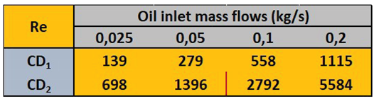
After the definition of the geometrical characteristics of the FOGVCs and the presentation of the approaches applied in this work, representative boundary conditions both in the oil and in the air domain have been defined. The worst case from the thermal point of view would take place when a predetermined part of the generated heat in the heat source can not be dissipated through the FOGVC provoking possible malfunctions. Considering the combination of thermo-fluid variables of the heat exchanger (inlet mass flows and temperatures), which define the FOGVC operation, low air mass flows (velocities) combined with low oil-to-air temperature differences and high oil mass flows have been investigated, Table 1.
On the oil side, the mass flow through every FOGVC can take values from 0,025 to 0,2 kg/s with a inlet temperature of C for all investigated cases. On the air side, the temperature (C), pressure (atmospheric pressure at the see level, 1 bar) and velocity (50 m/s) have been selected closed to the real boundary conditions established for the FOGV on the ground idle flight phase under the maximum hot day condition.
Here are two key points regarding the selected boundary conditions. On the oil side, the inlet mass flow range and oil inlet temperature were chosen based on preliminary analytical calculations aimed at studying laminar, transitional, and turbulent flows. On the air side, the heat transfer coefficient was selected based on simplified analytical calculations that encompass a broad range of values. The air temperature was determined by rounding the highest recorded temperature on Earth. To ensure low Mach numbers, an air velocity of 50 m/s was chosen, considering the defined characteristic length.
It is important to note that, depending on the level of simplification applied, different variables may be required for the setup of air conditions. For instance, in the high-fidelity L0 3D CHT simulations, inlet temperature, velocity, and pressure are utilized (left sub-table in Table 1). However, with a more simplified model, the setup only requires the inlet temperature of the bypass duct, used as the air free stream temperature, and the heat transfer coefficient (right sub-table in Table 1).
The comparison of the above methodologies at different levels of simplification and combined with the boundary conditions applied to 2 different concept designs contribute clearly to understand deeper the heat transmission and fluid mechanisms which take place in an oil-to-air Fan Outlet Guide Vane Cooler (FOGVC).
3. Analytical Assessments
The analytical assessments belong to the simplification level 3 (L3), only analytical equations and correlations based mainly on empirical results, are used to determine the pressure drop of the oil system and the heat transmission between the hot oil and the air, assuming strong simplifications.
3.1. Heat Transfer
In the determination of the transmitted heat within the heat exchanger and the oil outlet temperature, some simplifications have been used. By the first one, the flow over the FOGVC is idealized as a parallel flow over a flat plate, due to the low total thickness and relative angle of the flow respect to the curvature of the airfoil. The following simplification considers how heat is transferred between the two fluid domains. In this approach, heat transmission is treated as one-dimensional, occurring only perpendicular to the flat plate, while also accounting for partial dissipation through the lateral sides of the oil cavities. This quantification is obtained more exact in L0, L1 and L2. Regarding the heat transfer mechanisms used in this work, and due to the low oil-to-air temperature differences, the radiation heat transmission is considered negligible. The last simplification refers to the fact that the oil connections are only located in the root of the FOGVC and within the airfoil. Assuming for the L3 that the main heat exchange takes place through the airfoil, it is acceptable to use as dissipation area either the oil-metal interface, the metal-air interface or an average of both. The decision, which dissipation area is employed in the analytical correlations, has a big impact, as it will be shown later, in the dissipated heat and the oil outlet temperature.
The combination of the above simplifications allow to reformulate the 3D study in the FOGVC as a 1D steady-state metal wall analysis with the following heat transfer mechanisms: internal forced flow heat convection between the oil and the metal domain, conduction through the metal part and external forced flow heat conduction with the air. As no internal generation of thermal energy exists within the metal wall, and applying the energy conservation law to the simplified 1D plane wall, the total heat transfer rate in the FOGVC, , keeps constant through all interfaces , where and is the convective heat rate at the oil-metal and metal-air interface, respectively, and the conduction heat rate. Using the Newton’s law of cooling for the convective term,
and the Fourier’s law for the heat conduction,
where, h is the convection heat transfer coefficient ( and in the oil-metal and metal-air interface, respectively), A is the dissipation area, and L is the thermal conductivity and thickness of the solid domain, respectively, and the temperature difference between both interfaces, a general expression for the heat rate through the FOGVC is obtained as followed,
In the above equations, and represent the free stream temperature of the oil and air, respectively.
Applying an electrical analogy to the FOGVC thermal circuit, 3 thermal resistances can be identified on the equation 3: , and but only the can be calculated without further analysis because is composed of known variables. Moreover an overall heat transfer coefficient, U, can be defined based on the total thermal resistance of the wall plate. The main drawback of the equation 3 to determine the total dissipated heat and the outlet oil temperature is that the is unknown. An option to overcome that is the log mean temperature difference (LMTD) method [25], but due to its iterative nature, an alternative method is preferred. The number of transfer units (NTU) method solves this issue by relying only on the effectiveness of the heat exchanger, , the minimum heat capacity rate of the fluids, , and the temperature difference of the fluid at the inlets,
In the above equation, and represent the free stream temperature of the oil and air at the inlets, respectively.
Key factor by the NTU method is the determination of the effectiveness with values staying between 0 and 1. An alternative definition of for any heat exchanger [25] based on the heat capacity ratio, and the number of transfer units () is,
being the definition of as followed,
There are some expressions of the equation 5 available, depending mainly on the type of the heat exchanger (parallel- or counter-flow, shell-and-tube, cross-flow with simple pass) and on . In Table 2 the values of , and are summarized being the same for CD1 and CD2.
The results show that the air capacity rate is much larger than that of the oil, meaning that the air temperature remains almost constant after the FOGVC. Since the values of remain very close to zero, is assigned a value of zero. This allows the following equation to be used to assess the effectiveness, :
To confirm that the equation 7 is valid for our purpose, a comparison with -expressions for a counter-flow and a cross-flow with unmixed fluids heat exchanger has been made with differences under 1% confirming the validity of the assumption.
The last step to assess the heat transfer using the NTU method is the determination of the number of units of the heat exchanger using the equation 6. For that, the overall heat transfer coefficient, U, and the dissipation area should be assessed. Before the assessment of U is explained, the decision about which dissipation area is used for the 2 interfaces in the calculations is needed. As dissipation area can be used the oil-metal interface area (smallest area), , the average method proposed in [26]: , the arithmetic mean of the 2 interfaces: , or the metal-air interface area with the highest value, . In the Table 3 the total values for the CD1 and CD2 can be seen and the augmentation heat rate factors resulting by comparing the above proposed dissipation areas with the CAD’s measurement of the oil-metal interface, the smallest one.
The results show that the augmentation of the heat rate taking as reference the smallest area, , vary between 1.06 and 1.94 times by CD1 and between 1.03 and 2.53 times by CD2. By using , the highest augmentation factor is introduced in the calculations obtaining too optimistic heat rates, which could provoke malfunction and overheating in the heat source. One alternative would be , but as later shown by the numerical results (L0, L1 and L2), the heat dissipation is not only concentrated in the vicinity of the oil cavities but in an wider area, which means that and are better alternatives to be used. Due to the above reasons, is a good compromise for the thermal resistances, as the differences with A2 are insignificant.
The metal thermal resistances for CD1, , and CD2, , can now be assessed.
To calculate the heat transfer coefficient of the metal-air interface, , needed to determine the thermal resistance , the following expression is employed:
where represents the non-dimensional Nusselt number, the thermal conductivity of the air and x a characteristic length where the number is assessed. Nusselt convection correlations of an external flow over a flat plate, semi-empirical equations depending on the non-dimensional numbers and , are employed to determine the number. To determine the appropriate correlation for our problem, it is essential to identify the location on the airfoil where the flow transitions from laminar to turbulent. Using the recommendation of Incropera et al. [25] for external flows, this transition takes place where the , being , and the dynamic viscosity, the density and the free stream velocity of the air, respectively. For our airfoil, with a chord length of 0.2 m, the m is located very closed to the trailing edge. Hence, 2 possible Nusselt correlations can be used, assuming the use of average values for with m instead of local one:
By the equation 9, the average Nusselt number, , is assessed assuming a mixed flow. As the laminar flow is presented over circa of the whole chord length, an alternative Nusselt correlation for laminar flows can be used:
The assessment of the non-dimensional numbers and , being , the specific heat, is carried out as followed: the ideal gas law [27] is used to determine the air density, :
where R the ideal gas constant and and are the pressure and temperature of the air, respectively. By the air dynamic viscosity, , the Sutherland’s Law with 3 coefficients is used [27]:
taking the reference viscosity, , the value kg/ms and the reference temperature, . S is the effective temperature or Sutherland constant with a value of 110.56 K. The last two material properties of the air to be calculated are the specific heat, and the thermal conductivity . By the specific heat, a 3rd-degree polynomial function of T is used [27]:
where the coefficients and take empirical values. In the case of the thermal conductivity, , a parabolic function of T with empirical coefficients is used:
Knowing the above material properties for the air, the and number take the values 0.71 and , respectively and using the flat plate correlation for mixed flow, equation 9, a heat transfer coefficient of is obtained, presenting a difference of circa to the results obtained with the laminar correlation . In order to obtain a better understanding of the air side heat transmission, a range of between 50 and 150 instead of the above analytical values has been employed as boundary condition in the numerical simulations at levels L1 and L2, see Table 1. As the transition laminar-to-turbulent take places over the FOGVC surface, the heat transfer coefficient for mixed flow will be used to calculate the air thermal resistance, being and . Actually only one thermal resistance for the air side is needed, if the dissipation area is constant. In our case, the dissipation area is an average of the 2 fluid-solid interfaces making needed the assessment of a second thermal resistance for CD2.
The last thermal resistance to be determined corresponds to the internal flow in the oil side, . For that, a similar process, as by the external flow, is followed to assess but with some differences. Within the oil internal cavity, the fluid is confined by the oil-metal interface appearing two regions: entrance region (hydrodynamic and thermal) and the full developed region. In this work only correlations for fully developed flows are employed to simplify the calculations following the recommendations of Incropera et al. [25]. For laminar flows (), like in CD1 with all mass flows and by CD2 with 0.025 and 0.05 kg/s, when (in our case at the inlet), or by turbulent flows outside of the entry length, defined as , being the hydraulic diameter, this is a reasonable assumption. Another difference with the air side methodology, in which the is a constant, is that in the oil side an estimation of a mean temperature alongside the oil cavity, , is needed to evaluate the material properties of the oil due to the variation of the oil temperature from the inlet to the outlet. In this work, and using a constant surface temperature condition, an arithmetic mean temperature approach has been used, obtaining a mean oil temperature of C when supposed a oil outlet temperature of C. Moreover the oil used for this assessment is a common jet engine oil MIL-L-23699 (5cSt). Now it is possible to evaluate for the different mass flows, obtaining that only laminar flows are present by CD1, Figure 5. By CD2, turbulent flows appears clearly when the two highest mass flows are employed.

Table 4.
Oil Reynolds numbers corresponding to the analytical assessments using the arithmetic mean approach by CD1 and CD2.
Table 4.
Oil Reynolds numbers corresponding to the analytical assessments using the arithmetic mean approach by CD1 and CD2.
The values of the Nusselt numbers in laminar flows for pipes with circular cross section do not depend on the Reynolds numbers, being a constant, 3.66. By rectangular cross sections, the Nusselt number varies depending on the ratio . Ratios higher as 8 are considered as ’infinite’ ratio corresponding to a constant Nusselt number of 7.54 [25]. By turbulent flows, however, the Nusselt number are assessed using more complex correlations in which the roughness of the wetted surface and friction effect play an important role. In this work the correlation for smooth pipes is used and valid for the investigated range of Reynolds numbers, provided by Gnielinski [25]:
where is the Darcy friction factor [28], which depends on the flow regime, . For turbulent flows in smooth surfaces for circular pipes, in the range , three correlations can be employed: the correlation of Konakov [28]:
the Petukhov’s correlation [25]:
the correlation included in [28]:
or for a global range of , based on the values of the laminar and Konakov’s correlations [28]:
being defined for as:
In equation (20) an additional factor, , can be introduced [28] to take into account friction effects by rectangular cross sections like by CD1:
depends mainly on the ratio of the dimensions of the cross section () presenting a monotone decreasing behaviour, see Figure 6. For square cross sections (ratio = 1), the takes the lowest value, 0.89, provoking a reduction of the Darcy-factor of 11% in comparison with the circular cross section case. No impact of the geometric dimensions on the friction factor (=1) takes place when the ratio is equal to 0.44.
By the CD1 geometry with a geometrical ratio of 0.0727, the factor and the friction factor results 87.93. This value is lower as the proposed in [25], 96, by using the expression for laminar and rectangular cross sections:
In the next chapter, a comparison of the friction factor values obtained in equations 21 and 22 is conducted by assessing the pressure drop to estimate any potential influence on the fluid variables. However, this does not consider the impact on heat transfer, as the friction factor is not accounted for in the equations governing laminar flow.
Finally, all needed ingredients are known to assess analytically the total dissipated heat in the FOGVC (equations 3 and 4) and the outlet temperature of the oil for the predetermined boundary conditions. The following figures summarize the most important results of the analytical calculations. In the Figure 7, Figure 8 and Figure 9 can be seen the results by fixing the air heat transfer coefficient to the obtained value 73.2 . On the contrary, in the Figure 10 and Figure 11 the results show the influence of the air heat transfer coefficient in the range from 50 to 150 in the global thermal analysis.
The Figure 7, (left), shows the evolution and comparison of the dissipated heat depending on the oil inlet mass flow by CD1 and CD2. In CD1 the increment of the mass flow has a very low impact on the dissipation heat achieving a maximum improvement of only 40 W (from 467.7 to 508). By CD2, on the contrary, a clear improvement exists when the mass flow achieves the value 0.1 kg/s on which the laminar flow changes to transition one, obtaining maximum improvements of circa 105% (from 324.3 W to 663 W). The change of the behaviour between laminar and transition flows will be clearly shown in the following sections. The effect of mass flow increment on the outlet temperature can be seen in the right side of Figure 7, provoking a lower reduction of temperature descend between inlet and outlet. Remarkable is that neither of the concept designs are able to reduce the inlet temperature beyond C. In case that the lowest outlet temperature is the scope of the oil-to-air heat exchanger, CD1 fulfills this requirement, when the mass flows remain below 0.1 kg/s, hence, in laminar range.
The influence of different friction factor correlations over the oil convection heat transfer coefficient and the Nusselt number by turbulent flows in CD2 can be seen in Figure 8, (left). No significant differences (below 2% by and ) have been obtained by comparing the three correlations (Petukhov, Konakov and global range correlation) using the highest mass flow. The Petukhov’s correlation is employed for the rest of the analytical calculations as the values provided by the other 2 correlations are more extreme.
To optimize the thermal behaviour of the FOGVC, it is needed to know which side of the heat exchanger provokes a higher thermal resistance by the heat transmission. This information is presented by Figure 8, (right).
Using a constant heat transfer coefficient on the air side (), the thermal resistances of CD1 are represented in the most inner ring of the graphic, Figure 8 (left). Only 1 ring is needed by CD1 due to the laminar nature of the investigated flows. In this case with an air thermal resistance of 65.34%, the air side is restricting the heat dissipation coming from the oil side. Hence, the air side should be improve instead of the oil cavities, e.g by increasing the air velocity or the dissipation area, adding fins, etc.. In CD2 something similar is happening, but more extreme, by the most outer ring (0.2 kg/s) and the second more outer one (0.1 kg/s) with air thermal resistances over 90% (both transition flows in the oil side). The laminar cases of CD2 (0.025 and 0.05 kg/s), represented by the ring with values: oil= 53.34%, metal= 1.54%; air= 45.13%, is the only one in which the oil thermal resistance is higher than the air one but with values quite similar to the air side. A configuration with similar thermal resistances on both fluid sides is recommended to avoid bottlenecks by the heat dissipation. Regarding the conduction metal thermal resistances, all remain below 3% by both concept designs. The reduction of the metal resistance normally is related to structural issues, as to reduce this resistance it is needed to reduce the thickness of the oil-air wall and/or the increase of the thermal conductivity of the FOGVC material, which normally is not possible due to strength requirements.
To know the dissipation potential of the FOGVC, the effectiveness, , and the maximum possible heat transfer rate, , defined in the NTU method can be used, Figure 9.
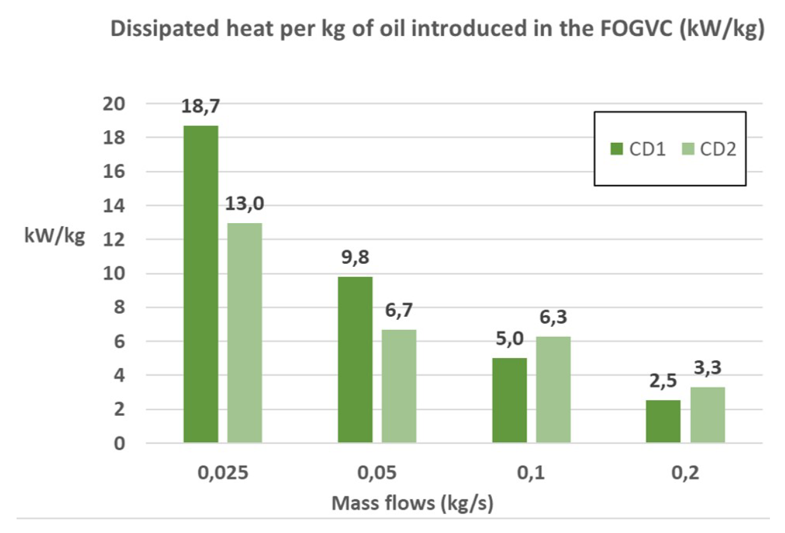
Based only on the heat capacities and the inlet temperatures of both fluids in the FOGVC, the theoretically maximum possible heat transfer rate, independent of the employed concept design, increases linearly with the mass flow, obtaining a maximum value of 21.4 kW, Figure 9 (right). If a heat exchanger is integrated in every FOGV, the theoretical total dissipation heat rate of the FOGVC assembly can achieve 856 kW (assuming 40 FOGVCs). Unfortunately the effectiveness of the FOGVC decreases with the increment of the mass flow and the type of design, as can be seen in the left graphic of the Figure 9, obtaining the total heat transfer rate multiplying both variables, see left graphic of Figure 7.
Until now a constant air heat transfer is employed. Now, the influence of the air heat transfer coefficient variation is investigated, Figure 10.
Regarding the dissipated heat rate by CD1, a slight continuous increase takes place, when the oil mass flow is augmented. A higher impact has the increment of the air heat transfer coefficient (from 50 to 150 ), provoking maximum improvements of circa 95% at the boundary condition BC12. By CD2 the transition from laminar to transition flows has a huge impact on the heat dissipation causing increments between 62% () and 158% (), achieving maximum heat rates of 1.25 kW (BC12). A similar behaviour can be observed by both concept designs when the results of the oil outlet temperature are shown (increase of the outlet temperature when the inlet mass flows increases too). The only exception happens when the mass flow is 0.1 kg/s, dropping the temperature slightly and increasing again with 0.2 kg/s, probably due to transition effects. If achieving the lowest outlet temperature after the FOGVC is the goal, only the lowest mass flow rate can meet this requirement.
The last analytical investigation dealt with the weighting ratios between the thermal resistances when the air heat transfer coefficient is modified, Figure 11. For CD1, the air thermal resistance predominates over the oil one by lower heat transfer coefficients, achieving a desired balance by (air: 47.9%; oil: 49.2%), when an oil inlet mass flow rate of 0.2 kg/s is employed. In the last case, the presence of bottlenecks in the heat dissipation are minimized. This is not the case by CD2, in which a balance between the air and oil thermal resistance is not achieved neither in the laminar nor in transition flows, being the weighting ratios by the transition case, around 90-10% with oil mass flows of 0.1 and 0.2 kg/s, much more unbalance as by the laminar one, 40-60%, where oil mass flows vary between 0.025 and 0.05 kg/s.
Figure 11.
Influence of the air heat transfer coefficient on the dissipated heat rate with an oil inlet mass flow rate of 0.2 kg/s (inner ring: ) (left) and on the outlet oil temperature (right) for the concept designs CD1 and CD2.
Figure 11.
Influence of the air heat transfer coefficient on the dissipated heat rate with an oil inlet mass flow rate of 0.2 kg/s (inner ring: ) (left) and on the outlet oil temperature (right) for the concept designs CD1 and CD2.
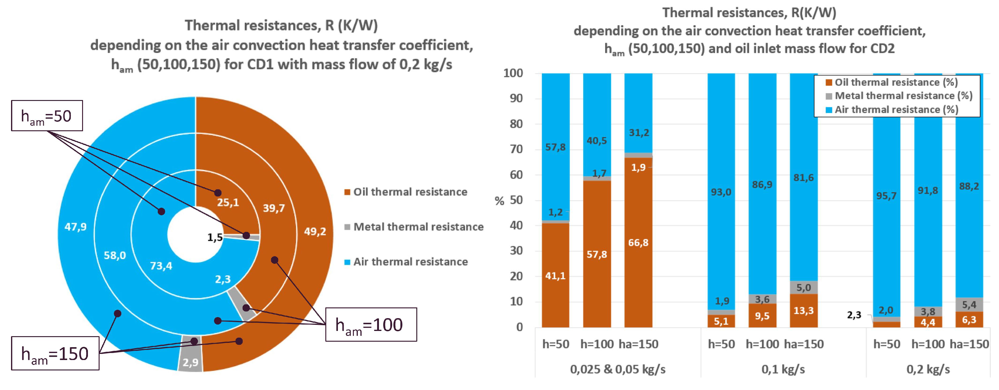
Figure 12.
Capacity of dissipation (kW/kg) depending on the inlet mass flow and the concept design.
3.2. Pressure Drop
The pressure drop in a hydraulic system can be defined as irreversible energy losses due to recirculation regions, separation and secondary flows and friction of the fluid with the walls. In a general form, and based on the relationship with the average kinetic pressure of the flow, the pressure drop definition of an hydraulic element, the Darcy-Weisbach equation (23), depends on geometrical dimensions of the oil cavity, length L and hydraulic diameter of the cross section , fluid properties, like the density and velocity v, and on the Darcy-friction factor , see equations (16)-(22):
For laminar flows in CD1 and CD2, using equations (20)-(22) and the definition of the Reynolds number (), the Darcy-Weisbach equation can be simplified to yield the Hagen-Poiseuille equation:
By comparing these two equations, a notable distinction between flow behaviors becomes evident. For laminar flow, the pressure drop exhibits a linear dependency on the velocity, whereas for turbulent flow, it follows a quadratic dependency, see Figure 13.
The last two equation are valid only for straight pipes and does not take into account pressure losses due to change of the flow directions, like by bends. As the two investigated concept designs have 180-degree bends, additional terms in the equation 25 are needed. Assuming that an hydraulic system is composed by hydraulic elements (straight pipes, bends,...), a general expression of the pressure drop presents the following form [28]:
The second term, the flow deflection loss, presents a similar form as the friction loss term. The only difference is the addition of the curvature effects through the ratio and the correction factor [28]:
where corresponds to the correction factor for bends. For -bends, used in the two investigated concept designs, the correction factor can be derived using the expression .
In Figure 13 can be seen the analytical results of the pressure drop of both concept designs.
In CD1 the pressure drop increases linearly due to the laminar nature of the flows (equations 22 and 23), remaining the maximum value below 8 kPa. Due to the cross section reduction in CD2, the pressure drop is clearly higher than CD1, achieving a peak of circa 341 kPa by the maximum mass flow. A change of the flow behaviours (from laminar to transition) can clearly be seen when a mass flow of 0.1 kg/s is achieved by CD2.
4. Numerical Setup
After the analytical calculations carried out in L3, the numerical setups used in the softwares ANSYS Fluent™, Flownex™ and ANSYS Mechanical™ for the simplification levels L0, L1 and L2 are explained.
4.1. ANSYS Fluent™
In the presented work the commercial software ANSYS Fluent™ 2020R2 is employed for 3D steady-state conjugate heat transfer and computational fluid dynamic simulations of the FOGVC. As the influence in the results by using different simplification level (L0, L1 and L2) is investigated, different setups are defined. In all simulations, the Navier-Stokes equations (continuity, momentum and energy) for the laminar flows in the oil domain and the Reynolds-averaged Navier-Stokes equations (RANS) applying the SST turbulence model for oil and air domain in turbulent flows are employed.
In both concept designs a mesh study of the simulation domains oil and metal for the simplification level L2 has been carried out using 3 level of mesh refinements (coarse-C, fine-F, ultra fine-UF), Table 5, to find a mesh which captures and models with enough precision the oil behaviour and the heat transmission without using unnecessary computational resources.
To correctly model the heat transfer mechanisms on the oil-metal-air interfaces, a refinement of the unstructured mesh including an inflation layer has been added. To avoid poor mesh quality elements, the coarsest refinement level has been established on a mesh with 5 millions control volumes on the oil domain. The fine and ultra-fine refinement levels were obtained by approximately doubling each immediately coarser level. A conformal mesh would be an option to model correctly the heat fluxes on the interface. The main disadvantage of this method is the unnecessary low size elements on the metal side. An alternative to this expensive method is a "quasi-conformal" mesh on which the mesh elements of the oil and metal domain do not coincide completely but an imposed growing mesh size factor, in our case of 1.75, is used to delimit the size of the elements on the metal side of the interface, taking .
To estimate the appropriate mesh refinement to be used in the simulations, a quantitative criterion, consisting of the comparison of pressure drop, outlet oil velocity, heat flux rate and oil outlet temperature in a steady state using the boundary condition BC3, has been employed, obtaining the following results, Table 6:
By the comparison of the different variables using the 3 mesh refinement levels and observing that the differences of the studied variables are below 1.2% and 0.5% in CD1 and CD2, respectively, the coarsest mesh has been selected for the remaining simulations. In L0 the mesh employed in the air domain is based on the application of a mesh size factor of 1.5 at the metal-air interface assuring good resolution of the boundary layer with a in the range 0-8, being a compromise between high accuracy and low computational times. The total size of the O-M-A meshes in L0 is of 68 and 65 millions of control volumes for CD1 and CD2, respectively. Some details of the meshes used in this work, mainly refinement zones and inflation layers, can be seen in Figure 14.
For the CHT and CFD simulations, some assumptions have been taken: the oil behaves like an incompressible and Newtonian fluid and no phase change takes place (single phase). Moreover an inertial non-accelerating reference frame is used and both body forces (Coriolis, centrifugal and gravitational) and radiation heat transfer are negligible.
Depending on the simplification level, the simulated domains and the associated set-ups are different, Figure 14. Starting with L2, only the oil domain (O) is simulated substituting the metal domain by a shell conduction model, in which a constant thickness of 3 mm and a thermal conductivity value depending on the temperature is applied, the air domain by a heat transfer coefficient and the air free stream temperature. At the oil inlet a constant mass flow and temperature boundary condition, see Table 1, with a turbulence intensity of 5% is employed while at the outlet the gauge pressure value is fixed. The no-slip condition is applied on the internal walls of the oil cavities. In L1 the setup for the oil domain is the same as by L2 but now the metal domain is simulated too and not substituted by the shell conduction model. In the new configuration (O-M), the same setup as in L2 is applied to the surfaces in contact with the virtual air domain, using an analytically calculated heat transfer coefficient and the air free-stream temperature. On the remaining surfaces (platforms on the top and bottom of the FOGVC) is employed an adiabatic boundary condition due to the expected low temperature gradient and heat transfer coefficients between the FOGVC surfaces and the surroundings (nacelle and core engine). Moreover a periodic symmetry condition is needed on the lateral surface of the lower platform as only one sector is simulated. In L0 no pre-assesed analytical calculations are needed to be applied on the external interfaces of the FOGVC, because the whole aero-thermo-fluid system (O-M-A) is simulated completely. The new boundary conditions to be defined are related with the air domain: adiabatic walls with no-slip condition on the top and bottom, a coupled metal-air interface, a periodic symmetry condition for the lateral surfaces and a pressure condition for inlet and outlet. The pressure condition at the inlet is composed of the application of a constant total pressure value of 102325 Pa, a constant temperature of C and the specification of the velocity components (tangential and axial) using the inlet total velocity value of 50 m/s and the relative angle to the axial direction of . As it is assumed that the flow after the fan does not contain the radial component, the associated angle is not needed. At the outlet a constant pressure condition of 101325 Pa is applied.
Regarding the flow solver, the pressure-based one is employed in L0, L1 and L2 to cover the range of low Reynolds numbers of the incompressible oil flow side (laminar and turbulent) and turbulent subsonic flow on the air side. As ANSYS Fluent™is conceived on a monolithic way, only one flow solver resolves both fluid domains in L0, and although the nature of the flows are completely different, the solver is able to achieve the convergence by stabilizing the pressure-velocity coupling. That means that there are cases in which the SST model is applied in laminar oil flows provoking eventually lack of accuracy of the results. The effect of using turbulence models in laminar oil flows may be investigated in future works. Together with the decay of the residuals below a predefined threshold ( in our research) of the continuity, velocity, energy and turbulent variables (k and ) additional convergence conditions have been applied, monitoring macroscopic variables in determined locations. For example, total temperature and pressure, mass flow and Reynolds number at the outlet and lateral heat transfer rate on the oil side, and the total mass flow on the air side have been monitored. Moreover the total heat transfer rate has been kept under surveillance. To be pointed out, in some cases the convergence has been achieved when the monitored variables stabilized without oscillations over the residual threshold is achieved and vice versa (the stabilization of the monitored variables take place below the residual threshold). Following the recommendations of ANSYS Fluent™ to improve the robustness, stability and convergence rate in the FOGVC [27,29], the coupled pressure-velocity solver is selected, in which the governing equations of momentum and pressure-based are solved together, instead of the segregated one, like SIMPLEC or PISO. For the evaluation of the gradients, used in the discretization of the diffusive and convective term, the by default least-squares cell-based scheme is applied. Moreover interpolation schemes of second order for the pressure and second order upwind for the rest of variables (momentum, energy, turbulent kinetic energy and specific dissipation rate in turbulent flows) are used. To stabilize the solution two types of under-relaxation factors are available on the coupled pressure-based solver: the explicit one, in which the update of the variables is controlled in every iteration, and the implicit one, based on the under-relaxation of the discretized equations [29]. The default explicit factors (0.5) for momentum and pressure are used in this work. The implicit under-relaxation factor depends on the CFL number (Courant-Friedrichs-Lewy), taking the value 200 by default. In our work the stabilization of the solver is achieved using CFL values between 25 and 50, depending on the flow (laminar or turbulent) and the simplification level. To be pointed out, the meaning of the CFL number used in this work is different to the CFL number defined in the convergence condition of explicit time-depending schemes. Before the simulations are started, hybrid initializations based on interpolation methods instead of the standard one, in which only constant values are selected, are carried out improving the initial values for the iterative solution process.
4.2. Flownex™
Instead of modeling the aero-thermo-fluid system using a 3D software like ANSYS FLUENT™, a 1D software at system and sub-system level, like Flownex™, can be employed to reduce the computational time at the expense of increased simplification [30]. In Flownex™ the one dimensional governing equations of conservation of fluid dynamics are the basis for the numerical solutions of thermo-fluid networks. Flownex™ obtains values of mass flow/velocity, pressure and fluid temperature by solving the conservation equations of mass, momentum and energy using the Newton-Raphson method and implicit pressure correction solution algorithm, see [26,31]. There are three solvers in Flownex™, each for pressure, flow and energy, using as convergence criterium for the residuals the value 1e-6.
Applying the work methodology of Flownex™ to the investigated concept designs by L2, Figure 15 shows, how the different parts of the FOGVC have been simplified using 1D components.
The metal domain is simplified to a pipe of certain thickness with the oil domain in the internal side and air domain in the external. The air side convection is applied to the outer area of the pipe. The input boundary condition required is the ambient air velocity, temperature and pressure. The hydraulic element of the setup is the pipe, a flow component of oil domain, where the length, hydraulic diameter and the details of the loss factors from the oil circuit is defined. In Flownex™ the input boundary conditions of the oil domain such as input temperature and pressure are entered in the input BC node (T P) and the mass flow in kg/s is provided in the output BC node (M). The component with red upward arrow marks is the composite heat transfer component, which acts as thermal component of the oil domain. This calculates the average temperature and convection coefficient caused by the flow in the pipe element. The fluid material properties have been added in the form of tables depending on the temperature. Regarding the bends and elbows, two different formulations are available: they are modeled using secondary losses with k factor or equivalent lengths or adding a component, as shown in Figure 15. Primary frictional losses "f" and the secondary losses "K" are integrated into momentum equation simulated in the pipe, the fluid flow component [32]. The pipe bend losses and pressure calculations on the oil side are also calculated similarly to the last section.
In thermal calculations, Flownex™ uses the Nusselt’s correlation to calculate heat transfer coefficient from air side using the external cylinder forced convection model. In the oil domain, inside the tube, the Gnielinski’s method is used for the convection transfer coefficient calculation. After calculating the convection transfer coefficients of both fluids, the energy equation is solved numerically until convergence.
4.3. ANSYS Mechanical™
In this part of the work, the commercial software ANSYS Mechanical™ is used by the simplification level L1 for conjugate heat transfer and fluid dynamic simulations of FOGVC. ANSYS Mechanical™ is a simulation tool which works on the principle of energy conservation using the Finite Element method (FEM). The heat balance equation is the basis for the thermal analysis obtained from the principle of energy conservation [33].
The geometry employed by the L1 simplification level is based on the replacement of the 3D oil body inside the circulating path with a 1D line element as shown in Figure 16 with an yellow highlight along the running length of the oil circuit. This 1D line has an attached cross section projecting along the length of the circulating path. This is achieved by assigning a uniform cross section to the 1D line body using the Design Modeller software in ANSYS Workbench™ [34].
The generated mesh is similar to the numerical setup in ANSYS Fluent™ in the case of metal domain and also in the oil-metal interface with an element size of 0.127mm. The only difference being in the oil domain mesh with edge sizing of 1D line body instead of 3D with an element size of 0.85mm. The area of the cross section of the oil domain is combined with the element size projected as a single 3D element for representation purpose. In this study we are assuming steady-state thermal simulations with incompressible fluid and non-linear material properties. ANSYS Mechanical™ contains variety of elements in its library applicable for structural, thermal, fluid, electric and magnetic analysis. The element type with suitable degrees of freedom (D.O.F.) decides the discipline of analysis. The library consists of one such suitable element known as FLUID116 for simulation of fluid domain in this work. FLUID116 is an element with two primary nodes capable of conducting heat and transmitting fluid between its primary nodes (I and J) and hence is a suitable option for the simulation conditions. Additional two nodes can be added for convection if desired. The material properties required are as follows, conductivity = KXX, density = DENS, coefficient of friction = MU , fluid viscosity = VISC and Specific heat = C. For convection analysis, the needed input parameters: D = hydraulic diameter and F = nodal heat or fluid flow rate in units mass/time. In this case, the film coefficient data is stored and is used by surface elements SURF 152. The SOLID87 is a 10 node, 3D tetrahedral solid thermal element used in metal domain and is very well suited for CAD-CAM system geometries consisting of unstructured mesh similar to our case [34].
The element programming in ANSYS Mechanical™ of FLUID116 does not support the calculation of fluid temperature, solid temperature and pressure loss calculation simultaneously. Hence, there is a need to perform two different simulation one to understand the thermal behaviour of solid with fluid and another for pressure loss in the fluid.
The steady-state thermal simulation consists of air-to-metal, metal-to-oil convection and temperature changes in oil and metal domains. The boundary conditions assigned to the metal surfaces on air side for convection is similar to L1 in ANSYS Fluent™ setup. The oil-metal convection coefficient is applied to the circuit walls and the temperature is taken from each 1D elements of fluid flow at corresponding locations. Mass flow for the 1D-oil line is applied in kg/s and fluid temperature at the first element of the inlet side. Thermal fluid is selected as model type in geometry and FLUID116 is assigned as element for the simulation [35]. The heat convergence value reference is 1e-5. There are the following points of interests regarding the results of the simulation: outlet temperature of the oil, temperature distribution on the surface of the metal and heat transfer between oil and metal as a result of convection.
The pressure simulation is also carried out in the steady-state thermal component of the ANSYS Workbench™ using ANSYS Mechanical™. Initial temperature is provided as in steady-state thermal analysis. The commands under the geometry tree help to change the analysis type from thermal to fluid by switching to the pressure DOF of element FLUID116. Then the details like hydraulic diameter and friction factor are added for each segment of straight line and bends. Further, commands applied under steady state thermal tree defines the boundary conditions like mass flow and initial pressure. Finally, commands are used to define the time steps which are basically iterations in steady state analysis since APDL works as a quasi-static type analysis [33]. The point of interest in this simulation are Reynolds`s number, fluid flow velocity in m/s and pressure difference between inlet and outlet of the oil circuit.
5. Numerical Results and Discussion
In this section, comparison of the numerical and analytical results belonging to the different simplifications levels are presented. Three variables are mainly investigated and compared: the oil outlet temperature, the dissipated heat rate from the oil to the air side and the pressure drop of the oil side. Another variables related with the three above are depicted, like the heat transfer coefficients on the oil-metal and metal-air interfaces, to understand better the influence of the used methodology.
Two types of results are presented: quantitatively, where the numerical results of the simulations are compared presenting absolute and relative values of the studied variables using the different approaches. The second type of results are the qualitative or visual ones, that means, a visual distribution of the studied variables are compared on the most important surfaces of the FOGVC, oil-metal and metal-air interface.
5.1. Computational Costs
The computational costs for each simplification level has been analysed. For the 3D conjugate heat transfer simulations at levels L0 and L1, performed using ANSYS Fluent™ , the cluster of the chair of Aeroengine Design was used. This cluster consists of 8 nodes with a total of 160 cores, though not all cores were always available, with a minimum of 80 cores dedicated to each simulation. For other simulations at simplification levels L1, L2, and L3, where ANSYS™ , Flownex™ , and/or analytical calculations were used, a local workstation with 8 cores was employed.
The duration of L0 simulations was typically under 60 minutes, although this varied significantly depending on the design concept and boundary conditions used (transitional or turbulent flow). In the 3D conjugate heat transfer simulations at L1, each simulation took no more than 15 minutes. The remaining L1 1D-3D simulations took much less time as the mapping of the heat fluxes at the interfaces was simplified strongly. For L2, Flownex™ 1D simulations were completed in a matter of seconds, while those in ANSYS Fluent™ took only a few minutes. Finally, the analytical calculations were completed within seconds.
5.2. Quantitative Results
The first results, Figure 17 and Figure 18, show the evolution of the outlet oil temperature depending on the inlet mass flow, the employed software and the two more extreme air heat transfer coefficients, 50 and (fixed by L1, L2 and L3). Moreover the differences of the results fixing the heat transfer coefficient on the air side on and taking the L0 as the reference method are depicted.
By CD1, the oil outlet temperature increases continuously by increasing the inlet mass flow, being framed on the range C. On the contrary, the differences with the reference level L0 decrease by all employed softwares, having a maximum difference of 5% (mass flow of 0.025kg/s), when Flownex™ is used. The same tendency is observed by CD2, Figure 18, obtaining a maximum deviation of circa 9% (ANSYS Mechanical™and Flownex™), by the lowest mass flow. With some exceptions (in CD1 the two lowest mass flows and in CD2 the two highest flows with transition/turbulent behaviour) are the results of L0 overestimated by the other methods being the results using more accurate (closer to L0) than the results of . In CD2, the change from laminar to transition/turbulent flows has a clear impact on the outlet temperature provoking a slight decrease (from 0.5 to 0.1 kg/s). No large deviations are expected by the outlet temperature due to the small range of temperatures obtained.
The results of dissipated heat are now depicted, Figure 19 and Figure 20. In CD1 and CD2, the values of the different methods underestimate the results of L0 with some exceptions (CD1: lowest mass flows. CD2: turbulent flows). Moreover the same tendency (the higher mass flows, the higher the dissipated heat) is observed.
Regarding the differences with the reference level L0, it can be seen in CD1 that they increase with the exception of the lowest mass flow. To be added is that the deviations are larger than by the outlet temperature (until 45% can be achieved using ANSYS Mechanical™ with the highest mass flow). Comparing the different softwares, ANSYS Fluent™(L1-O-M) obtains the closest results to L0 presenting maximum deviations of circa 15%.
The results in CD2 repeat the previously mentioned behaviour by augmenting the mass flows achieving maximum values of over 65% (ANSYS Mechanical™ by 0.1kg/s). A clear increment of dissipated heat takes place at mass flows of 0.1 kg/s and at the same time the deviations are reduced considerably.
The pressure drop is the last variable to be commented, Figure 21 and Figure 22. As expected, in CD1 a linear behaviour of the pressure drop in the whole laminar range can be seen, when a method is used, which is based on analytical equations. With the numerical methods, mainly 3D CFD, this behaviour changes to quasi-linear or even parabolic. This evolution becomes clear in CD2, Figure 22, when the mass flows achieves transition-to-turbulent structures.
While the pressure drop in CD1 remains in very low values (under 10000 Pa), the pressure range of CD2 varies strongly with the increment of the mass flow achieving values near to 4 bar. As explained before, the main reason is, although both concept designs present a similar hydraulic diameter, the lower cross section of CD2, which provokes higher velocities and hence pressure losses. Moreover the high number of bends contributes negatively. Examining the deviations related to the reference level, L0, in CD1, Flownex™ and the analytical method present the maximum values (50% and 25%, respectively). In case of Flownex™ , the main reason for that is the correction of the cross section applied in the bend. In CD2, the maximal deviations appear mainly at laminar flows, decreasing strongly when the transition-to-turbulent flow are predominant.
5.3. Qualitative Results
After the quantitative result comparison depicted in the last figures, a qualitative comparison is presented now.
The different investigated levels of simplification are presented, starting with the most precise and computationally expensive, L0-O-M-A, of both concept designs, Figure 23, Figure 24, Figure 25 and Figure 26.
Figure 23 shows the temperature distribution on the metal-air interface (top view), when the oil inlet mass flow increases, from 0.025 kg/s (BC1) to 0.2 kg/s (BC4). The higher the inlet mass flow, the lower the time for cooling the oil by the air and the bigger the area with higher temperatures. As expected, the highest temperature is located closed to the oil inlet, at the bottom of the FOGVC. The heated area on the metal-air interface is not only limited to the projected wetted area of the oil domain but increases in relationship with higher mass flows, as can be seen at the bottom of the FOGVC and in the cross section located in the middle of this figure.
The leading edge is almost not affected by the high temperatures in the most of the cases. The same happens close to the trailing edge but with the difference at BC4, that the cooling effect of the air is not able to reduce the oil temperature significantly alongside the whole radial direction until the bend. The top of the FOGVC maintains low temperatures in contrast to the other simplifications levels, as later will be shown. Inspecting the oil-metal interface (bottom view), the temperature distribution along the internal cavity shows a reduction until the bend is achieved, as the fluid flows mainly parallel to the internal surfaces with low number of whirls. Within and after the bend the secondary flow provokes an increment of the whirls increasing significantly the chaotic movement of the fluid and accordingly the surface temperature. Regarding the areas with high temperature gradients, these are located mainly at the bottom of the FOGVC and at the bend and clearly, at BC4, alongside the whole radial cavity after the inlet.
At CD2, Figure 24, the behaviour of the heated area is similar with the exception that after every bend the secondary flows reactivates the whirls increasing locally the temperature. From a thermomechanical point of view, this concept may increase the areas with high temperature gradients, forcing to the structural reinforcement of these regions and consequently increasing the weight of the whole FOGVC. As shown by the qualitative results at BC4, the air is not able to reduce significantly the oil temperature due to the high velocity of the hot oil.
Next, the heat transfer coefficient distribution is presented on the oil-metal and metal-air interfaces, Figure 25. As these distributions have been obtained using a numerical conjugate heat method with a fine mesh on both sides of the interfaces, the results are assumed to be the most precise obtained at all. Moreover, the heat transfer coefficient can be investigated locally, providing a high accuracy of the locations, where high temperature gradients appears. By the BC4 (0.2kg/s of oil inlet mass flow), where the differences between locations are clearly perceptible, in CD1 (left view) the maximum heat transfer coefficient is located at the bottom of the FOGVC closed to the inlet, coinciding with the maximum temperature areas. To be noted is the maximum value of the heat transfer coefficient, circa . This peak value is quite far away from the range of the analytical results, confirming the invalidity of them if a high accuracy regarding location and peak value is needed. This deviation takes place too by comparing with the dissipated heat, Figure 19, but not with the oil outlet temperature with a deviation of circa 1°C, Figure 17. At the oil-metal interface there are 2 regions with the highest value of the heat transfer coefficient, at the inlet, not a representative value due to numerical instabilities, and after the bend, achieving values of . At the CD2, metal-air interface, happens similar to CD1 with peak values of located mainly at the first pipes after the inlet. Considering the oil-metal interface, the highest values are located again at the inlet and in every bend with peak values between 3000 and due to secondary flows. In the straight pipes between the bends the transfer coefficient decreases to achieve the lowest value of around .
To finish the investigation of the L0 (O-M-A), the behaviour of the air flow is shown presenting as key variable the total velocity, Figure 26. The cooling effect of the air and the heated region after the trailing edge of both concept designs have been already presented, see Figure 23 and Figure 24. It can been observed that the air heated region after the trailing edge does not exceed a chord length in none of the studied cases. This is not the case if the total velocity is investigated. The FOGVC wake is perceptible from the trailing edge of the FOGVC to the air outlet (circa 1.5m downstream), presenting the tip corner vortex a bigger region with low velocities as the hub corner vortex. This is an important information to avoid undesired interactions with the surface air cooled oil cooler (SACOC), which usually is located after the FOGVC either on the outer or inner by-pass duct annulus. A reduction of the FOGVC wake may be obtained optimizing the aerodynamical FOGVC profile used in this study, as the present one has only a constant cross section, see Figure 3. A similar behaviour of the air is obtained by CD2, achieving air velocity peak values of circa 75 m/s, detail of the Figure 26.
An influence of the heat transmission from the FOGVC to the air in the by-pass duct regarding a variation of the Specific Fuel Consumption (SFC) has not been taken into account in this study but a significant influence is not expected.
After the presentation of the most accurate level, L0, the results of L1 (O-M) using ANSYS Fluent™ and ANSYS Mechanical™ are explained and compared. Starting with ANSYS Fluent™ , Figure 27, and using the conclusions of the quantitative results, Figure 17 and Figure 19, the boundary conditions presenting the lowest differences with L0 are BC9-BC12 (). High similarities are found with regard to the temperature distribution on the air-metal interface, see Figure 23. The main differences are presented by the higher mass flows and located at the bend and at the inlet radial oil cavity. The effect of the secondary flows within the bend is clearly higher by L1 while by L0 the temperature decreases constantly until the bend and not so abrupt as seen by L1 (CD1-L1-BC12). Moreover the heated area on the metal-air interface is limited to, approximately, to the projected area of the oil cavity and not extended, for example, to the trailing edge, as seen by L0. The boundary conditions BC5-BC8 are added to offer a comparison with the effects obtained with lower air heat transfer coefficient ().
The results of ANSYS Mechanical™ do not offer a better temperature distribution over the metal-air interface as the previous results, due to the fact that peak values and their locations are quite far away from the expected one or not represented clearly, Figure 28.
To finish the qualitative results, the temperature distribution at level L2 using ANSYS Fluent™ is presented, Figure 31. A similar temperature distribution is shown by L1 with the same differences with the level L0. With low mass flows, the oil is quickly cooled before the bend is achieved. When the oil mass flow increases, from 0.5 kg/s up, the influence of secondary flows within and after the bends are stronger as before.
6. Conclusions
In this work 0D-1D-3D and fully 3D steady-state aero-thermo-fluid simulations of a structural oil-to-air Fan Outlet Guide Vane Cooler (FOGVC) in a jet engine are presented. Using the commercial software ANSYS Fluent™, the thermo-mechanical module of ANSYS™ and the 1D fluid solver Flownex™, 5 simulation types (3D fully conjugate heat transfer with and without a thin wall model, 3D with a thin wall model, 1D-3D coupled, 1D and 0D) corresponding to 4 levels of simplification in 3 possible domains (oil, oil-metal and oil-metal-air) have been compared to provide a selection criteria when a determined level of accuracy in the simulations without prohibited computational times is desired. The methodologies are applied to two different oil internal cavities: an inverted U with rectangular cross section and a coil internal cavity with a circular cross section. The obtained results show that depending on the scope of the research, the investigated concept design and the oil inlet boundary conditions, one method or the other may be used.
If an accurate outlet oil temperature is needed, for both concept designs the differences with the most accurate method, ANSYS Fluent™ with the whole oil-metal-air model (L0 level), remain under 10%, meaning that the analytical methodology provides the best accuracy-to-speed ratio (only some seconds per calculation). As higher mass flows, these differences stay even below 2%. The main difficulty by using analytical and numerical methods, in which the heat transfer coefficient is a needed input, is its correct determination, since it could invalidate partially or totally the thermo-fluid results. In case that for the whole range of studied mass flows the highest accuracy is needed but a L0 simulation is out of the question, the L1 (O-M) using ANSYS Fluent™ is a possible option. At concept design 1 (CD1) the analytical method is still the best alternative to the most computational expensive method. As for CD2 the oil flow moves from a laminar to a turbulent regime by increasing mass flows, a correct calculation to the whole range is a challenge. In case that the dissipated heat is the key variable to be investigated, an adequate and accurate alternative would be again the L1 (O-M) ANSYS Fluent™ method. Comparing the pressure drop research results, at CD1, high deviations using the analytical and the FLOWNEX™ methods can be achieved, being recommended to use ANSYS Fluent™ to obtain higher accuracy. For CD2 in the turbulent regime all methods provide low deviations, under 12%.
At system level, the results of the analytical level would be an acceptable first estimation. When thermo-mechanical analysis are needed to determine locally the temperature distribution, L2 is not able to simulate the metal domain and L1 could not capture correctly the needed level of accuracy locally, meaning that the L0 is the only available method.
A key conclusion of this study is that relying solely on heat exchangers, which are passive components, makes it challenging to optimize the dissipation capabilities of aero jet engines operating under extreme and variable conditions. Conversely, active or adaptive components present a promising alternative to the current generation of heat exchangers.
Experimental data would be needed to validate the numerical results by all employed methodologies and geometries.
Future investigations may be focused on extreme boundary conditions like under very low temperatures, decongealing event, and possible malfunctions of the oil pump. Transient effects and mechanical analysis may be an important field of research too. Moreover the interaction between FOGVC with other oil components, belonging to the fluid system, and with other types of heat exchangers in the by-pass duct, e.g surface air cooled oil cooler (SACOC) will be an important area of investigation, as shown briefly by the air results.
Sample Availability: The data presented in this study are available partially on request, under certain conditions, from the corresponding author.
Author Contributions
Conceptualization: L.C.S; methodology: L.C.S; simulations FLOWNEX and ANSYS APDL: S.S.B.; simulations ANSYS Fluent: L.C.S.; meshing: L.C.S. and S.S.B.; investigation: L.C.S.; writing–original draft preparation: L.C.S. and S.S.B.; writing–review and editing: L.C.S. and K.H.; visualization: L.C.S.; supervision: L.C.S.; project administration: K.H.; funding acquisition: K.H. All authors have read and agreed to the published version of the manuscript.
Funding
The APC has received funding from the European Union’s Horizon 2020 research and innovation program under grant agreement No 690808 (project Surface Heat Exchanger for Aero Engines 2 - SHEFAE2).
Acknowledgments
The authors of this work are deeply grateful to the associate professor Fernando Varas Mérida (ETSIAE-UPM) for his technical support by the numerical simulations and comments.
Conflicts of Interest
The authors declare no conflict of interest. The founding sponsors had no role in the design of the study; in the collection, analyses, or interpretation of data; in the writing of the manuscript, and in the decision to publish the results.
Abbreviations
The following abbreviations are used in this manuscript:
| APDL | ANSYS Parametric Design Language |
| BC1 | Boundary Condition 1 |
| CAD | Computer Aided Design |
| CAM | Computer Aided Manufacturing |
| CD1 | Concept Design 1 |
| CFL | Courant–Friedrichs–Lewy number |
| CFD | Computational Fluid Dynamic |
| CHT | Conjugate Heat Transfer |
| DOF | Degree Of Freedom |
| FEM | Finite Element Method |
| FOGV | Fan Outlet Guide Vane |
| FOGVC | Fan Outlet Guide Vane Cooler |
| FVM | Finite Volume Method |
| IR | Intercooled Recirculated (gas turbine) |
| IT | Infrared Thermography |
| LC | Thermochromic Liquid Crystal method |
| LMTD | Log Mean Temperature Difference method |
| L0 | Simplification Level 0 |
| LPT-OGV | Low Pressure Turbine Outlet Guide Vane |
| NACA | National Advisory Committee for Aeronautics |
| NTU | Number of Transfer Units method |
| O | Oil domain |
| O-M | Oil-Metal domain |
| O-M-A | Oil-Metal-Air domain |
| PISO | Pressure-Implicit with Splitting of Operators algorithm |
| RANS | Reynolds-averaged Navier-Stokes equations |
| SACOC | Surface Air Cooled Oil Cooler |
| SGV | Structured Guide Vane |
| SIMPLEC | Semi-Implicit Method for Pressure Linked Equations-Consistent algorithm |
| UHBPR | Ultra High By-Pass Ratio |
References
- Climate change: what the EU is doing, 2023, https://www.consilium.europa.eu/en/policies/climate-change/, accessed on 2023-12-20.
- Royce., R. Royce., R. Future of flight., https://www.rolls-royce.com/media/our-stories/innovation/2016/advance-and-ultrafan.aspx, accessed on 2021-06-02.
- Commission., E. Commission., E. Horizon 2020., https://ec.europa.eu/programmes/horizon2020/en, accessed on 2021-05-25.
- Commission., E. Commission., E. Horizon Europe., https://ec.europa.eu/info/research-and-innovation/funding/funding-opportunities/funding-programmes-and-open-calls/horizon-europe_en, accessed on 2021-05-25.
- Royce., R. Royce., R. UltraFan. The Ultimate TurboFan., https://www.rolls-royce.com/~/media/Files/R/Rolls-Royce/documents/civil-aerospace-downloads/High-Res-posters/high_res_ultrafan.pdf, accessed on 2021-03-03.
- Venkataramani, K.S.; Moniz, T.O.; Stephenson, J.P. Heat transfer system and method for turbine engine using heat pipes. EP EP188 02, 2008.
- Wood, T.H.; Wetzel, T.G.; Luedke, J.G.; Tucker, T.M. Combined acoustic absorber and heat exchanging outlet guide vanes. US US833 12, 2012.
- Knight III, G.; Lukovic, B.; Laborie, D.; Scheffel, K.S. Gas turbine engine airfoil integrated heat exchanger. US US861 12, 2013.
- Gerstler, W.D.; Kostka, J.M.; Rambo, J.D.; Moore, J.W. Gas turbine engine component with integrated heat pipe. EP EP308 10, 2016.
- Snyder, D.J. Fluid cooling system integrated with outlet guide vane. US US2017029 10, 2017.
- Chalaud, S.; Vessot, C. Turbomachine provided with a vane sector and a cooling circuit. US US2018008 03, 2018.
- Zaccardi, C.; Boutaleb, M.L.; Chalaud, S.C.; Lemarechal, E.P.G.; Papin, T.G.P. Output director vane for an aircraft turbine engine, with an improved lubricant cooling function using a heat conduction matrix housed in an inner duct of the vane. US US1039 08, 2019.
- Sennoun, M.E.H. OGV heat exchangers networked in parallel and serial flow. US US1019 02, 2019.
- Wang, L.; Sundén, B.; Chernoray, V.; Abrahamsson, H. Endwall Heat Transfer Measurements of an Outlet Guide Vane at On and Off Design Conditions. Volume 3C: Heat Transfer; American Society of Mechanical Engineers: San Antonio, Texas, USA, 2013. [Google Scholar] [CrossRef]
- Wang, C.; Wang, L.; Sundén, B.; Chernoray, V.; Abrahamsson, H. An Experimental Study of Heat Transfer on an Outlet Guide Vane. Volume 5B: Heat Transfer; American Society of Mechanical Engineers: Düsseldorf, Germany, 2014. [Google Scholar] [CrossRef]
- Wang, C.; Luo, L.; Wang, L.; Sundén, B.; Chernoray, V.; Arroyo, C.; Abrahamsson, H. Experimental and numerical investigation of outlet guide vane and endwall heat transfer with various inlet flow angles. International Journal of Heat and Mass Transfer 2016, 95, 355–367. [Google Scholar] [CrossRef]
- Rojo Perez, B.M. Aerothermal Experimental Investigation of LPT-OGVs. PhD Thesis, Chalmers University of Technology, Gothenburg, Sweden, 2017. [Google Scholar]
- Jonsson, I.; Chernoray, V.; Dhanasegaran, R. Infrared Thermography Investigation of Heat Transfer on Outlet Guide Vanes in a Turbine Rear Structure. International Journal of Turbomachinery, Propulsion and Power 2020, 5, 23. [Google Scholar] [CrossRef]
- Ito, Y.; Inokura, N.; Nagasaki, T. Conjugate Heat Transfer in Air-to-Refrigerant Airfoil Heat Exchangers. Journal of Heat Transfer 2014, 136, 081703. [Google Scholar] [CrossRef]
- Ito, Y.; Nakanishi, H.; Fukazawa, K.; Nagasaki, T. Geometric effect on heat transfer of airfoil heat exchanger. Asian Congress on Gas Turbines ACGT2016;, 2016; p. 9.
- Raatikainen, R.; Nousiainen, R.; Österberg, K.; Riddone, G.; Samochkine, A.; Gudkov, D. Applying one-dimensional fluid thermal elements into a 3D clic accelerating structure. CERN Open; CERN (European Organization for Nuclear Research): Geneva, 2010. [Google Scholar]
- van Antwerpen, H.J.; Mulder, E.J. A Technique to Simulate a Tube Break in a High-Pressure Gas/Cooling Water Heat Exchanger. Fourth International Topical Meeting on High Temperature Reactor Technology, Volume 1; ASMEDC: Washington, DC, USA, 2008; pp. 667–675. [Google Scholar] [CrossRef]
- Nouri, B.; Kuhhorn, A. Automated CAE process for thermo-mechanical lifing prediction of a parameterized turbine blade with internal cooling. 1th World Congress on Computational Mechanics (WCCM XI) 5th European Conference on Computational Mechanics (ECCM V) 6th European Conference on Computational Fluid Dynamics (ECFD V;, 2014; p. 16.
- Airfoil Tools, 2021, http://airfoiltools.com/, accessed on 2021-04-16.
- Incropera, F.P.; DeWitt, D.P.; Bergman, T.L.; Lavine, A.S. (Eds.) Fundamentals of heat and mass transfer, 7. ed., ed.; John Wiley & Sons, Ltd: Hoboken, NJ, 2011. [Google Scholar]
- Flownex. Flownex Library Manual. Version 8.10. 2019.
- Baker, T.J. Ansys Fluent User’s Guide 2020R2. 2020.
- Wagner, W. Strömung und Druckverlust: mit Beispielsammlung, 5 ed.; Vogel: Würzburg, 2001. [Google Scholar]
- Abrahamson, J. Ansys Fluent Theory Guide 2020R2. 2020.
- Flownex®, SE. TUTORIAL 6 - Heat Exchanger, 2019.
- Flownex®, SE. Flownex® SE, https://www.flownex.com/legacy/information/capabilities/solver, accessed on 2019. Flownex® SE.
- Flownex®, SE. Flownex Theory Manual, 2019.
- ANSYS, Inc.. ANSYS Mechanical APDL Thermal Analysis Guide, 2017. Ansys® Academic Research Mechanical, Release 18.1, Help System, Steady-state thermal analysis, ANSYS, Inc.
- ANSYS, Inc.. ANSYS Mechanical APDL Element Reference, 2013. Ansys® Academic Research Mechanical, Release 15.0, Help System, Coupled Thermal-Fluid Pipe, ANSYS, Inc.
- ANSYS, Inc.. FLUID 116 EXAMPLE, 2016. Ansys® Academic Research Mechanical, 2016, ANSYS, Inc.
Figure 1.
The FOGV assembly is located in the by-pass duct of an aero engine downstream of the fan between the fire zone 1 (nacelle) and 2 (core engine) (picture adapted with permission from [5]).
Figure 1.
The FOGV assembly is located in the by-pass duct of an aero engine downstream of the fan between the fire zone 1 (nacelle) and 2 (core engine) (picture adapted with permission from [5]).
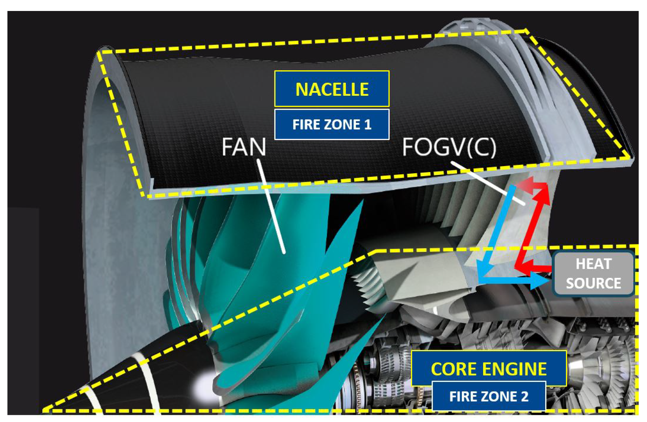
Figure 2.
Geometrical dimensions of a simplified bypass duct-FOGVC assembly dimensions used in the simulations.
Figure 2.
Geometrical dimensions of a simplified bypass duct-FOGVC assembly dimensions used in the simulations.
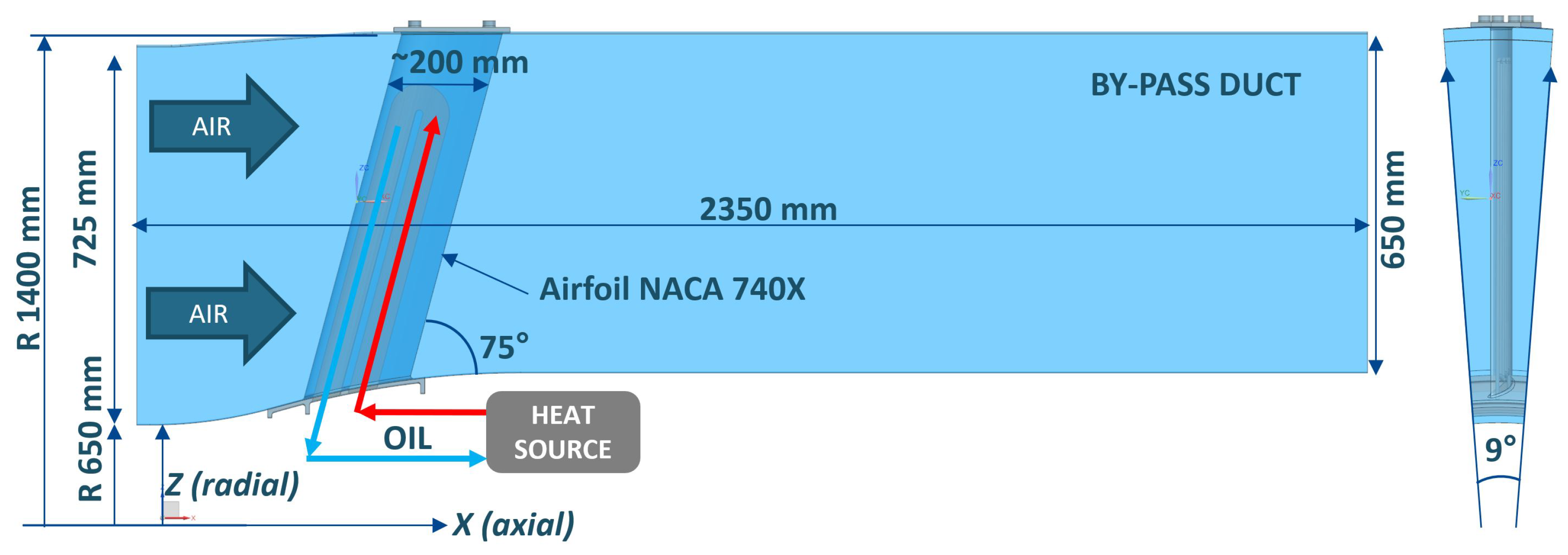
Figure 3.
Geometrical dimensions of the investigated concept designs: the concept design 1 (CD-1) presents an inverted U with rectangular cross section (4mm x 55mm) meanwhile by the concept design 2, a coil internal cavity with a 7.5mm diameter circular cross section (CD-2) has been used presenting 8 straight pipes and 7 -bends.
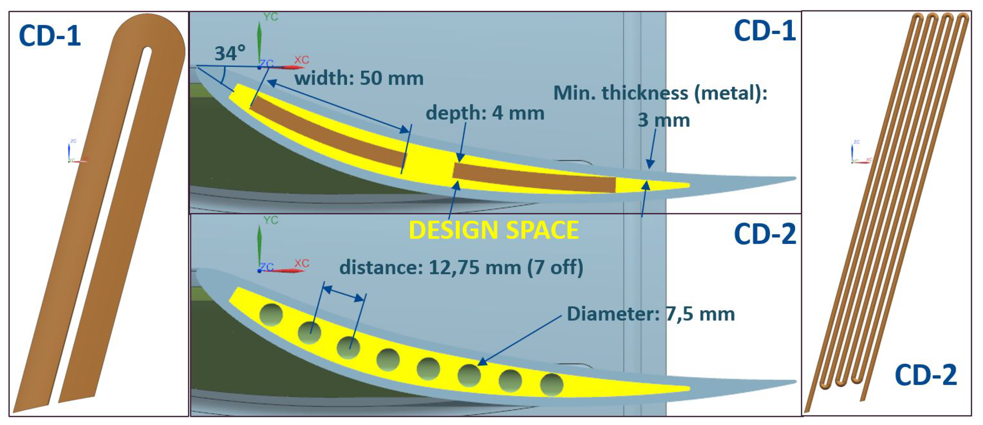
Figure 4.
Approaches employed in this work: 5 simulation types (3D fully conjugate heat transfer (CHT) with and without a thin wall model, 3D with a thin wall model, 1D-3D coupled, 1D and 0D) corresponding to 4 levels of simplification in 3 possible domains (oil, oil-metal and oil-metal-air) have been compared.
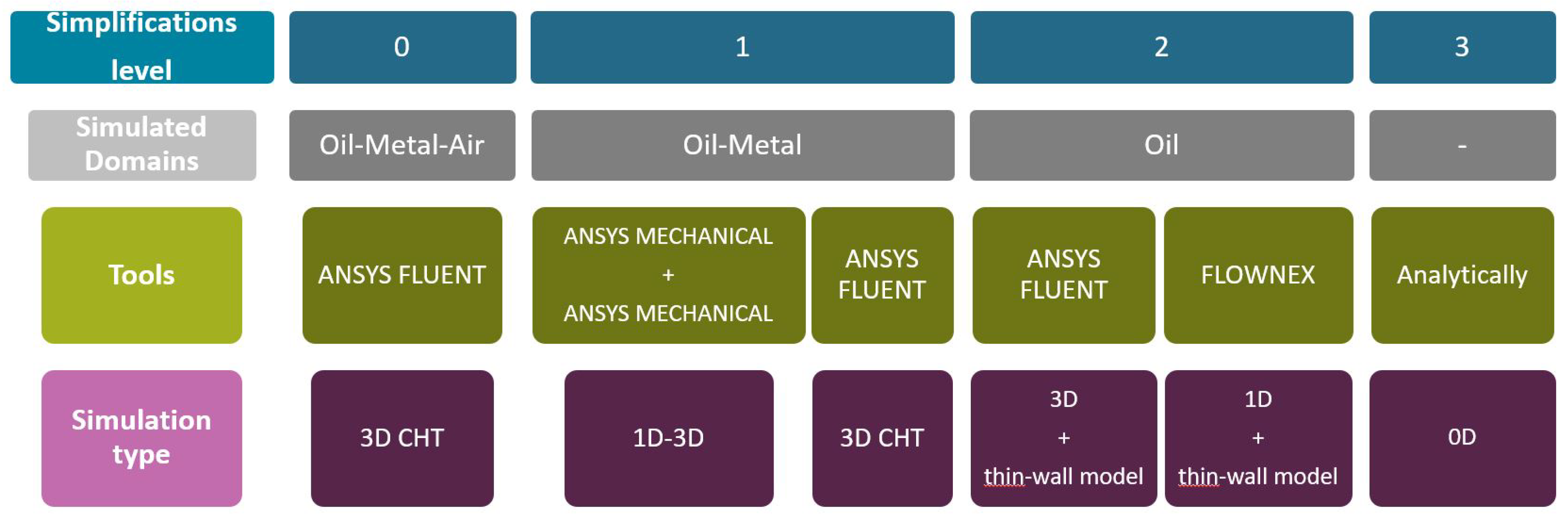
Figure 5.
Oil Reynolds numbers corresponding to the analytical assessments using the arithmetic mean approach by CD1 and CD2.
Figure 5.
Oil Reynolds numbers corresponding to the analytical assessments using the arithmetic mean approach by CD1 and CD2.
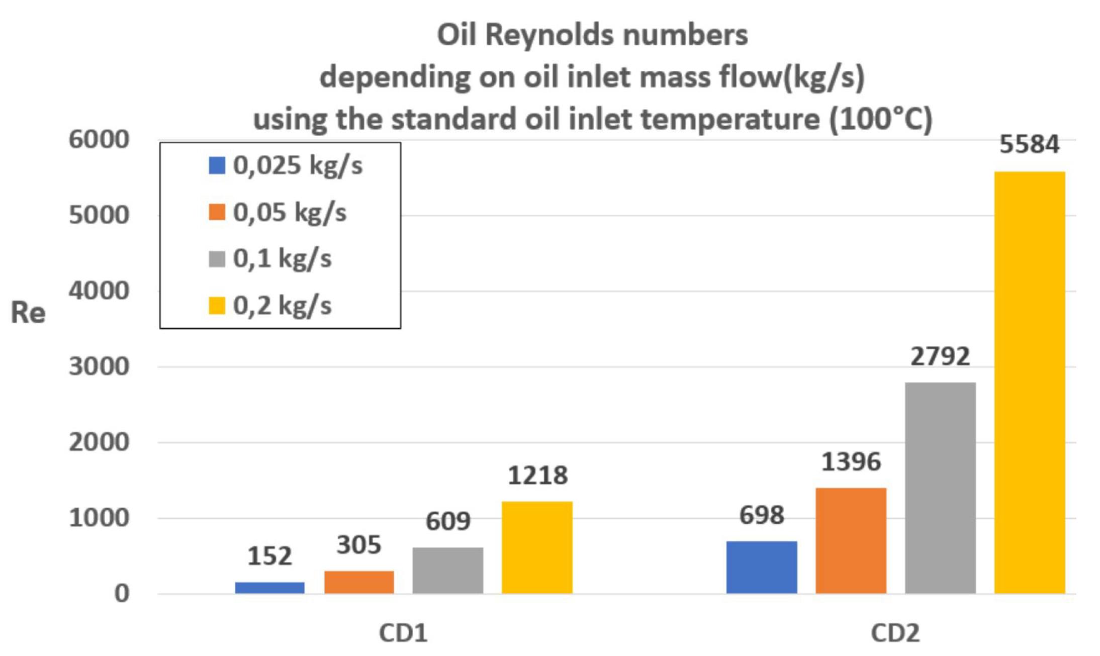
Figure 6.
Influence of the geometric dimensions of the cross section over the Darcy-friction factor in laminar flows , (based on Figure 70 by [28]).
Figure 6.
Influence of the geometric dimensions of the cross section over the Darcy-friction factor in laminar flows , (based on Figure 70 by [28]).
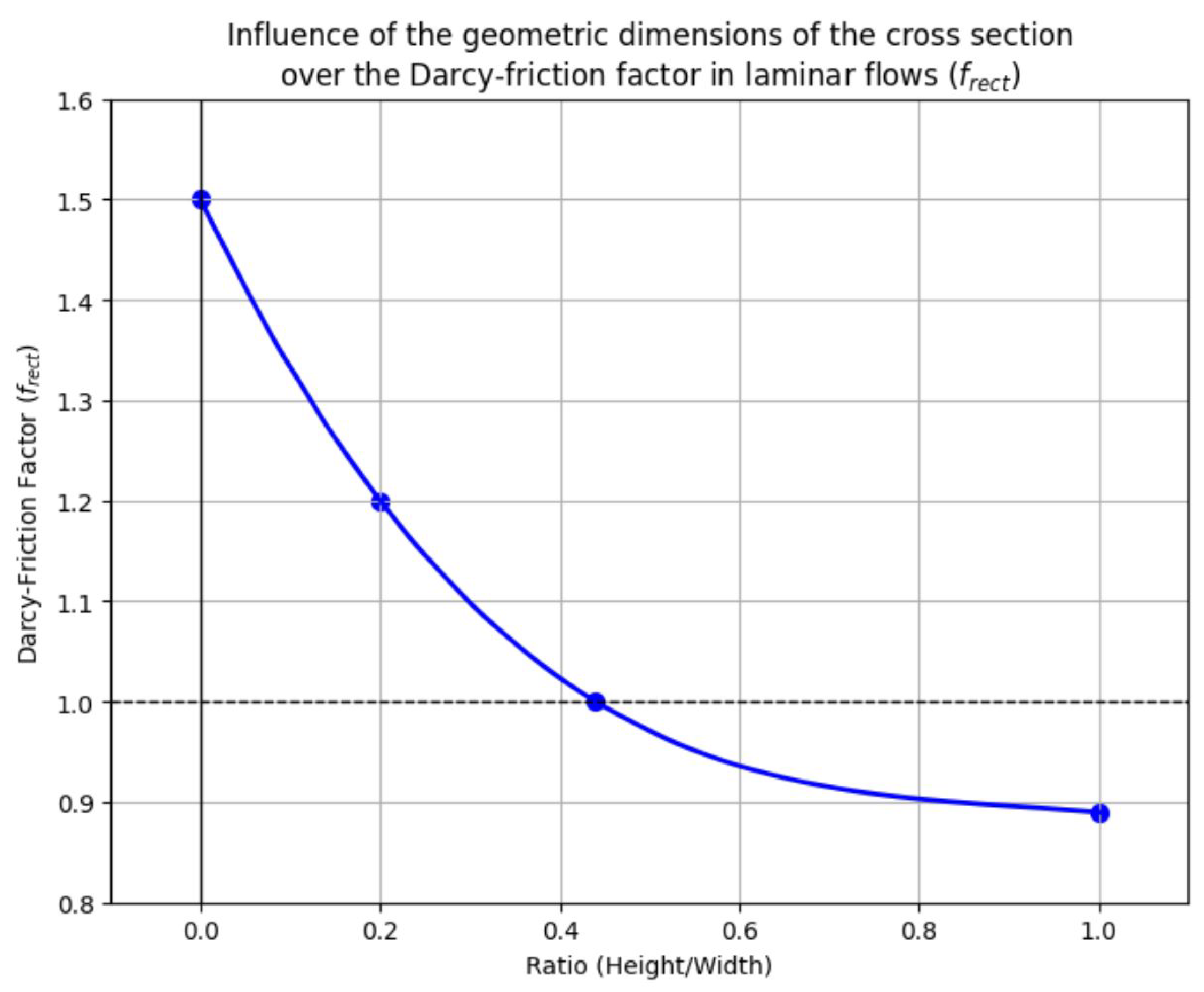
Figure 7.
Comparison of the dissipated heat (left) and the outlet oil temperature (right) using by CD1 and CD2 depending on the feeding oil mass flow rates.
Figure 7.
Comparison of the dissipated heat (left) and the outlet oil temperature (right) using by CD1 and CD2 depending on the feeding oil mass flow rates.
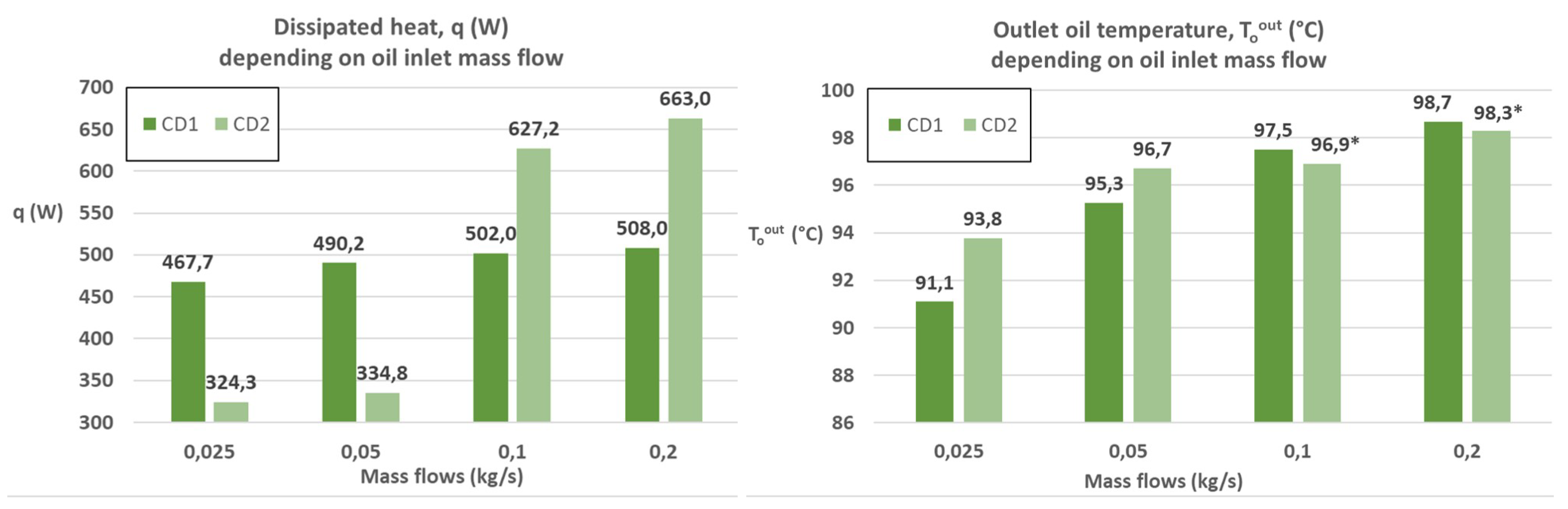
Figure 8.
Comparison of the influence of different friction factor correlations over the oil convection heat transfer coefficient by turbulent flows in CD2 (left) and thermal resistances of the CD1 (only one ring is needed, the most inner one, to represent the laminar flow regime in the whole range of investigated mass flows) and CD2 (three outer rings are needed: the first most inner represents the constant thermal resistances by the laminar flows: 0.025 and 0.05 kg/s, and the two most outer corresponds to the turbulent flows: 0.1 and 0.2 kg/s, respectively) using as friction factor the Petukhov’s correlation and (right).
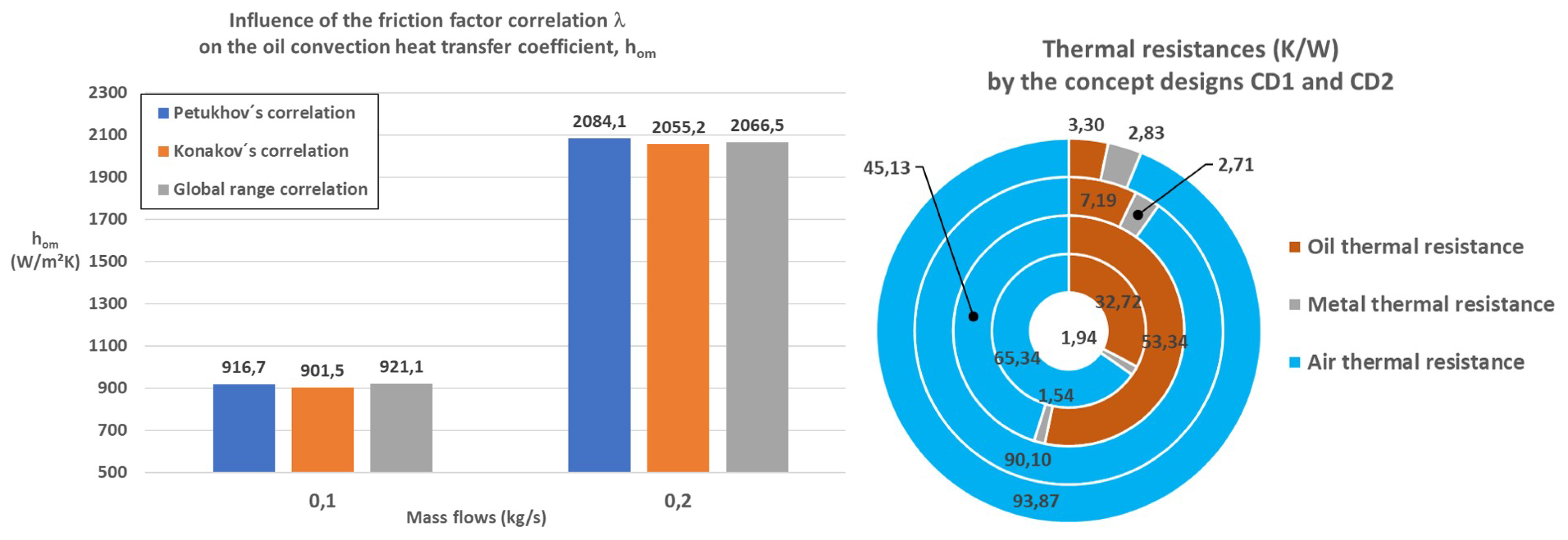
Figure 9.
Effectiveness (%) (left) and maximum possible heat transfer rate, (right) of the concept designs CD1 and CD2.
Figure 9.
Effectiveness (%) (left) and maximum possible heat transfer rate, (right) of the concept designs CD1 and CD2.
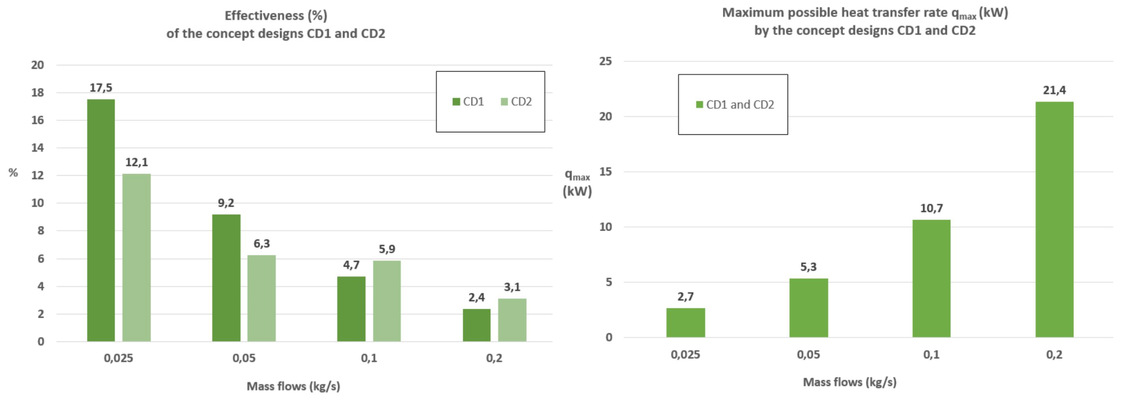
Figure 10.
Comparison of the evolution of dissipated heat (left) and outlet oil temperature (right) depending on the oil inlet temperature, mass flow and air heat transfer coefficient by the concept designs CD1 and CD2.
Figure 10.
Comparison of the evolution of dissipated heat (left) and outlet oil temperature (right) depending on the oil inlet temperature, mass flow and air heat transfer coefficient by the concept designs CD1 and CD2.
Figure 13.
Pressure drop of CD1 and CD2 depending on the oil inlet mass flow with a fixed oil temperature of 100°C. (Note: The graphic on the right uses piecewise linear segments rather than a smooth curve in the transition and turbulent range. Review the values to identify where the linear relationship transitions to a quadratic one.)
Figure 14.
Different set-ups associated to the simplification levels L2, L1 and L0 (top) and mesh details (bottom) applied in this work by CD1, when ANSYS Fluent™ is used.
Figure 14.
Different set-ups associated to the simplification levels L2, L1 and L0 (top) and mesh details (bottom) applied in this work by CD1, when ANSYS Fluent™ is used.
Figure 15.
1D Flownex™ diagram of the hydraulic, thermal and aero analysis of CD1 in simplification level L2. The diagram by CD2 is similar but having 22 hydraulic and thermal components (8 straight pipes + 14x-bends).
Figure 15.
1D Flownex™ diagram of the hydraulic, thermal and aero analysis of CD1 in simplification level L2. The diagram by CD2 is similar but having 22 hydraulic and thermal components (8 straight pipes + 14x-bends).
Figure 16.
Geometry of the concept design 1 (CD1) used by the L1 simplification level employing a 1D line at the center of the oil cavity.
Figure 16.
Geometry of the concept design 1 (CD1) used by the L1 simplification level employing a 1D line at the center of the oil cavity.
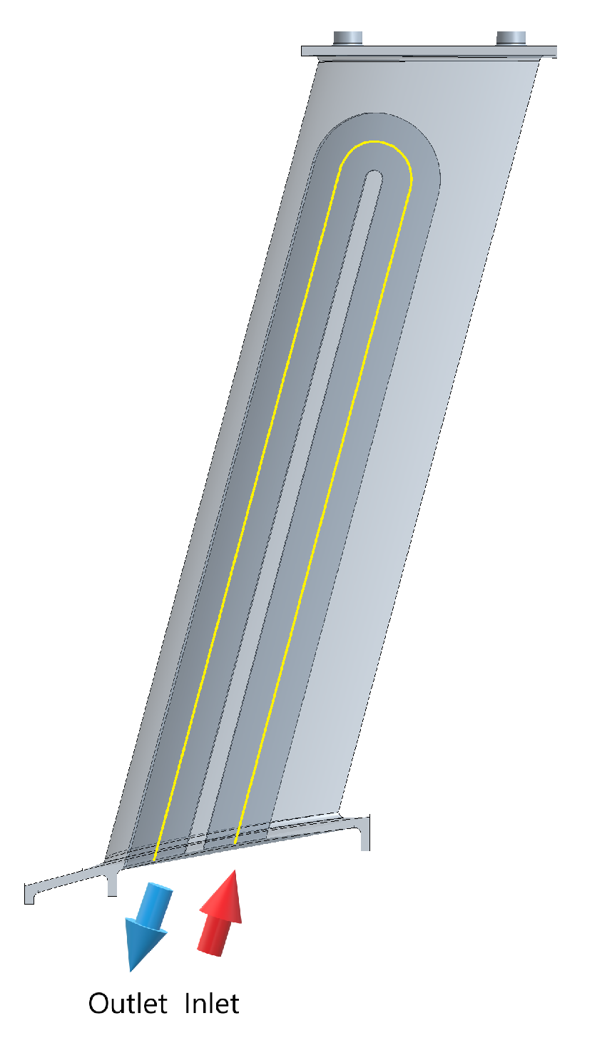
Figure 17.
Comparison of the oil outlet temperature results (left: absolute values, right: deviations respected to the L0 level) between the different simplification levels in CD1.
Figure 17.
Comparison of the oil outlet temperature results (left: absolute values, right: deviations respected to the L0 level) between the different simplification levels in CD1.
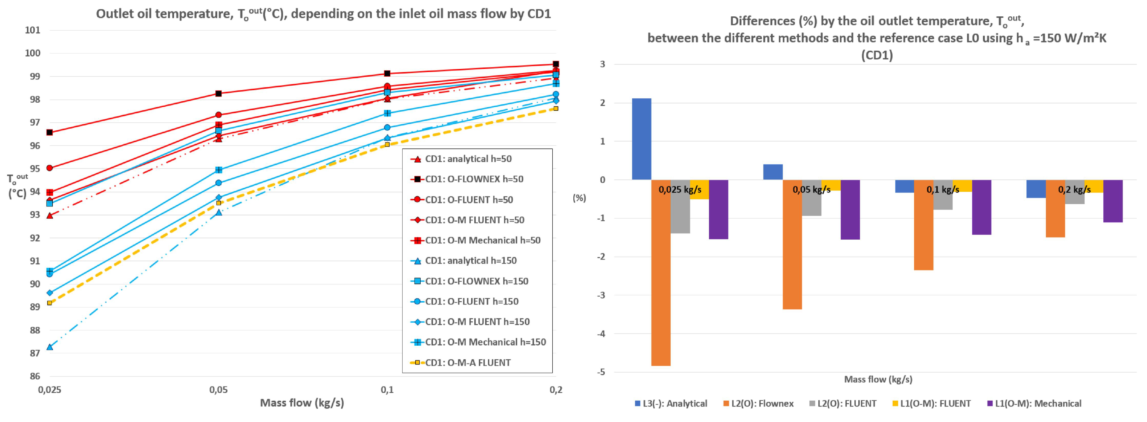
Figure 18.
Comparison of the oil outlet temperature results (left: absolute values, right: deviations respected to the L0 level) between the different simplification levels in CD2.
Figure 18.
Comparison of the oil outlet temperature results (left: absolute values, right: deviations respected to the L0 level) between the different simplification levels in CD2.
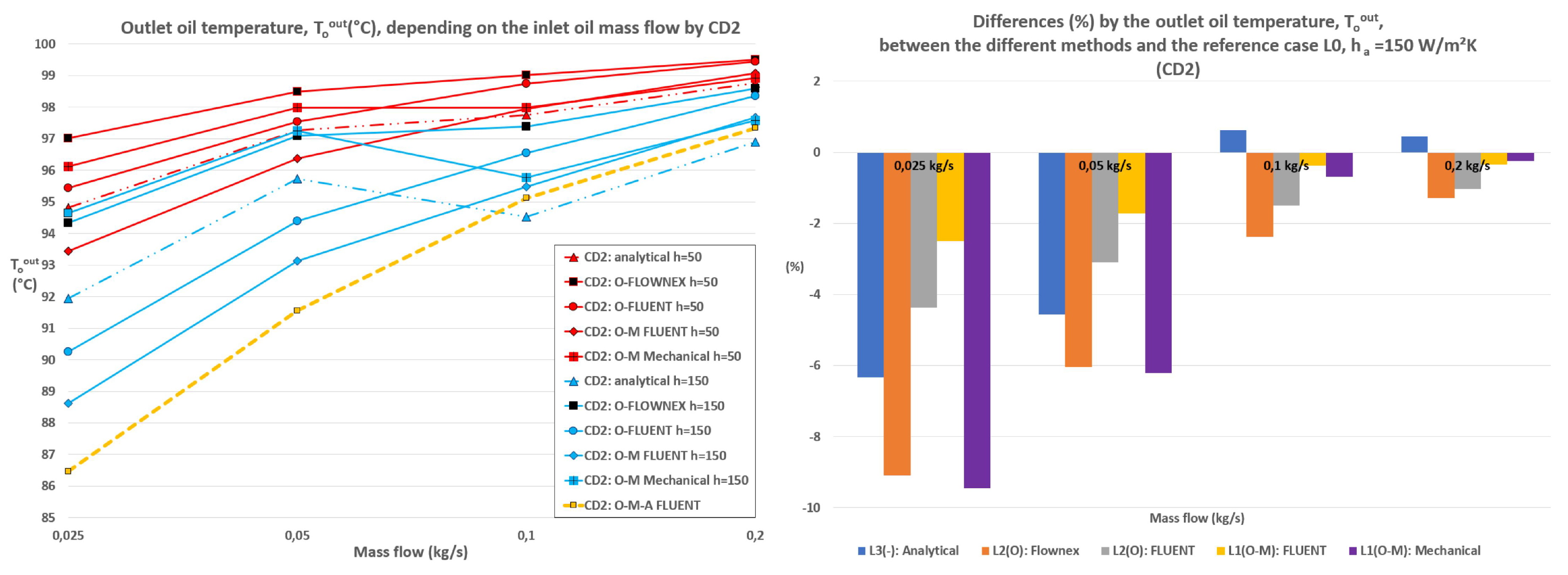
Figure 19.
Comparison of the dissipated heat results (left: absolute values, right: deviations respected to the L0 level) between the different simplification levels in CD1.
Figure 19.
Comparison of the dissipated heat results (left: absolute values, right: deviations respected to the L0 level) between the different simplification levels in CD1.
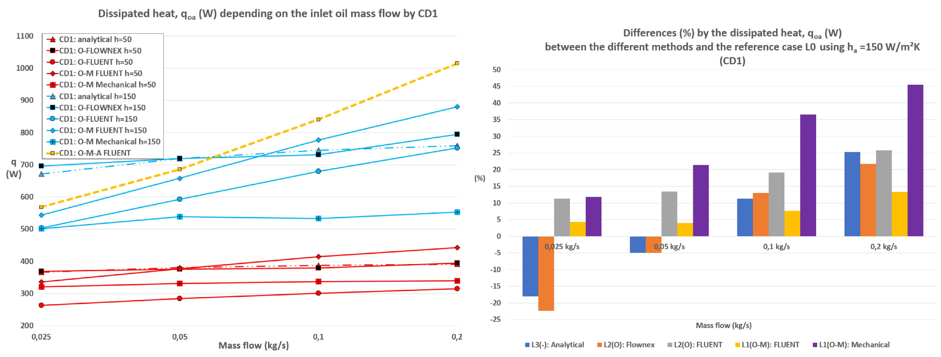
Figure 20.
Comparison of the dissipated heat results (left: absolute values, right: deviations respected to the L0 level) between the different simplification levels in CD2.
Figure 20.
Comparison of the dissipated heat results (left: absolute values, right: deviations respected to the L0 level) between the different simplification levels in CD2.
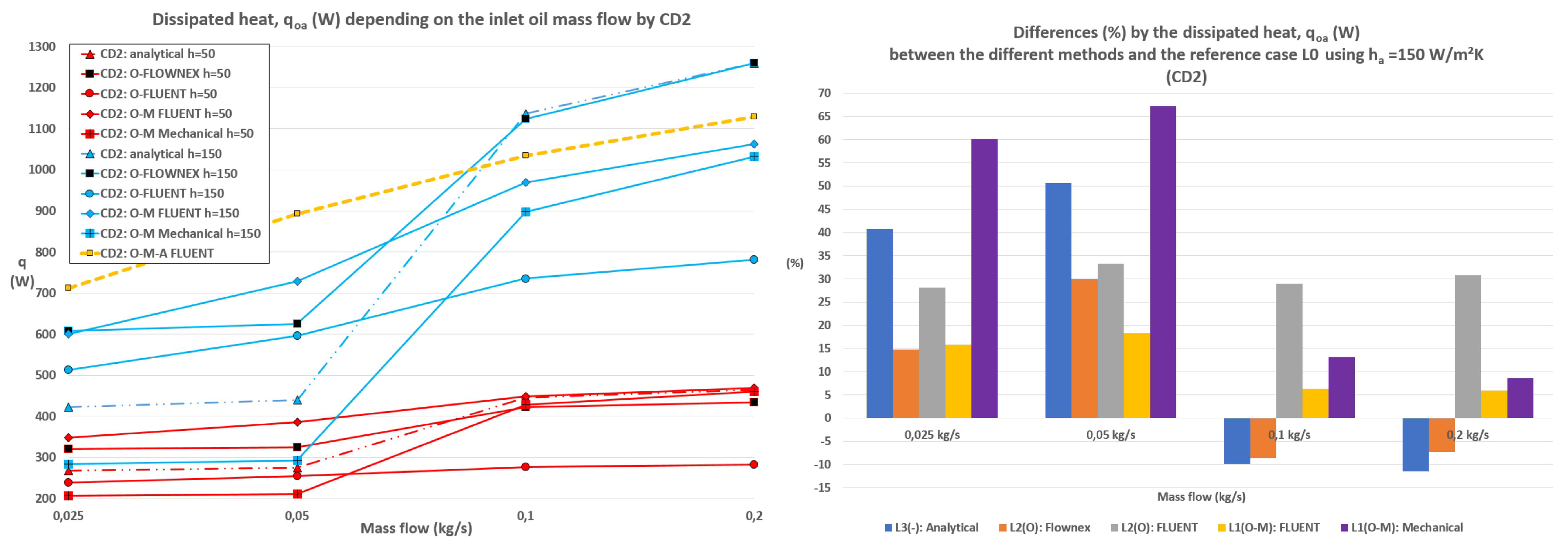
Figure 21.
Comparison of the pressure drop results (left: absolute values, right: deviations respected to the L0 level) between the different simplification levels in CD1.
Figure 21.
Comparison of the pressure drop results (left: absolute values, right: deviations respected to the L0 level) between the different simplification levels in CD1.
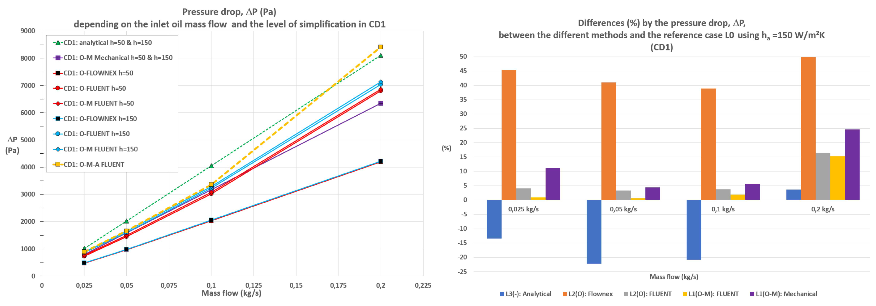
Figure 22.
Comparison of the pressure drop results (left: absolute values, right: deviations respected to the L0 level) between the different simplification levels in CD2.
Figure 22.
Comparison of the pressure drop results (left: absolute values, right: deviations respected to the L0 level) between the different simplification levels in CD2.
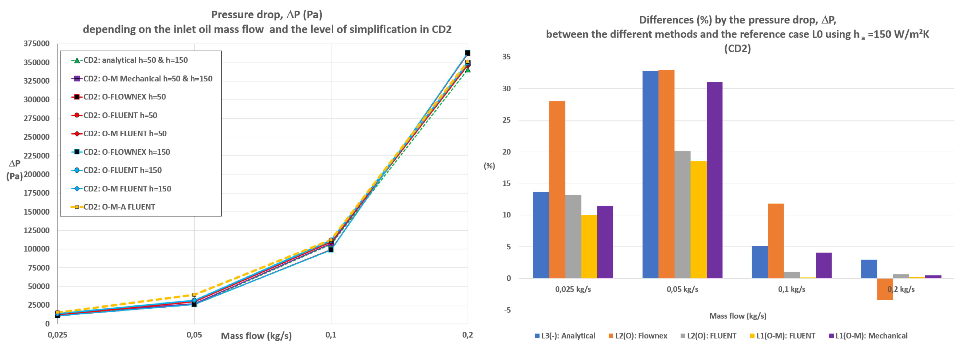
Figure 23.
Temperature distribution of CD1 at level L0 (O-M-A) for the boundary conditions BC1, BC2, BC3 and BC4. (Top view): metal-air interface; (middle view): bottom of the FOGVC, detailing the oil inlet and outlet; (bottom view): oil-metal interface and detail of an axial cross section at z=1.25 m.
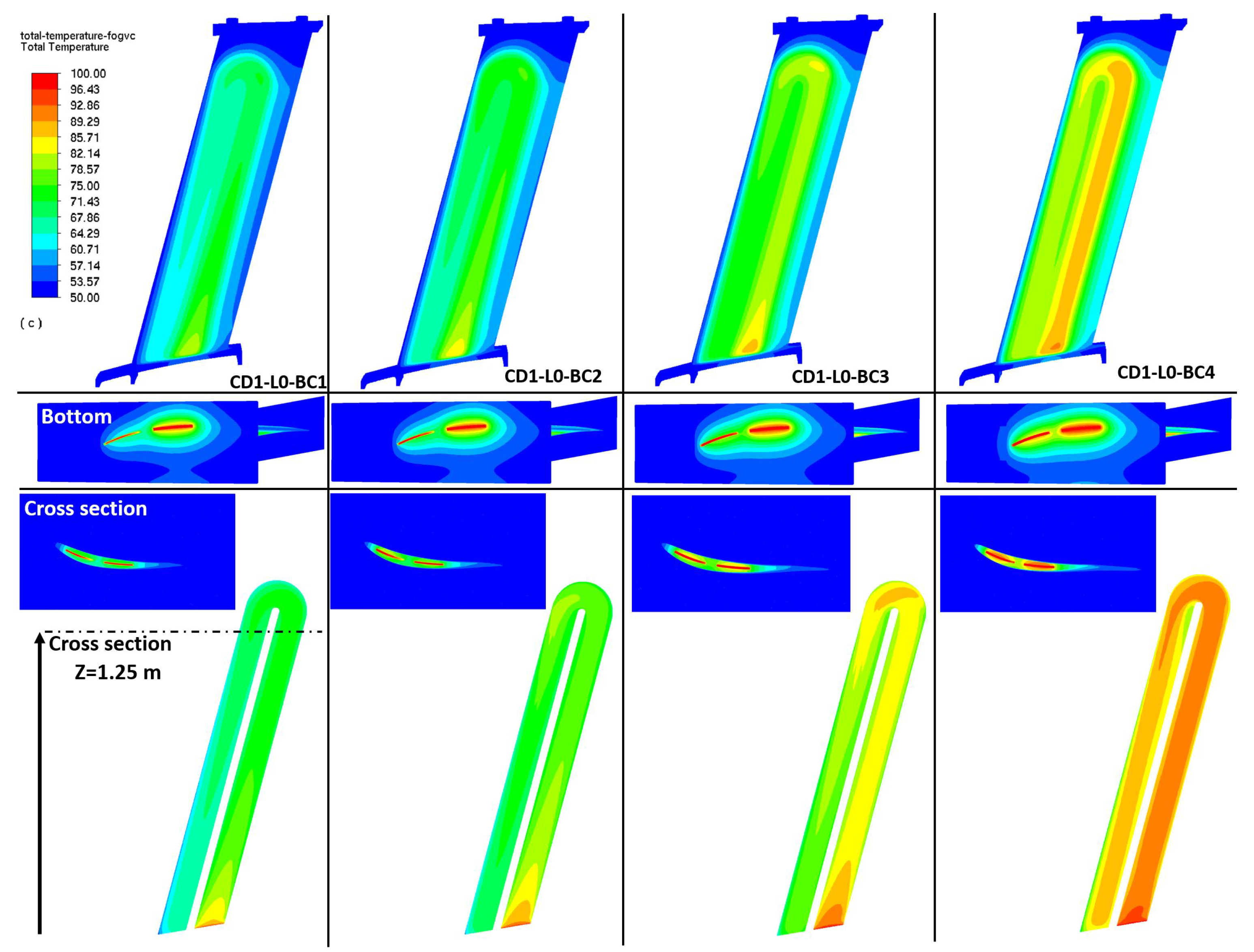
Figure 24.
Temperature distribution of CD2 at level L0 for the boundary conditions BC1, BC2, BC3 and BC4. (Top view): metal-air interface; (middle view): bottom of the FOGVC, detailing the oil inlet and outlet; (bottom view): oil-metal interface and detail of an axial cross section at z=1.25 m.
Figure 24.
Temperature distribution of CD2 at level L0 for the boundary conditions BC1, BC2, BC3 and BC4. (Top view): metal-air interface; (middle view): bottom of the FOGVC, detailing the oil inlet and outlet; (bottom view): oil-metal interface and detail of an axial cross section at z=1.25 m.
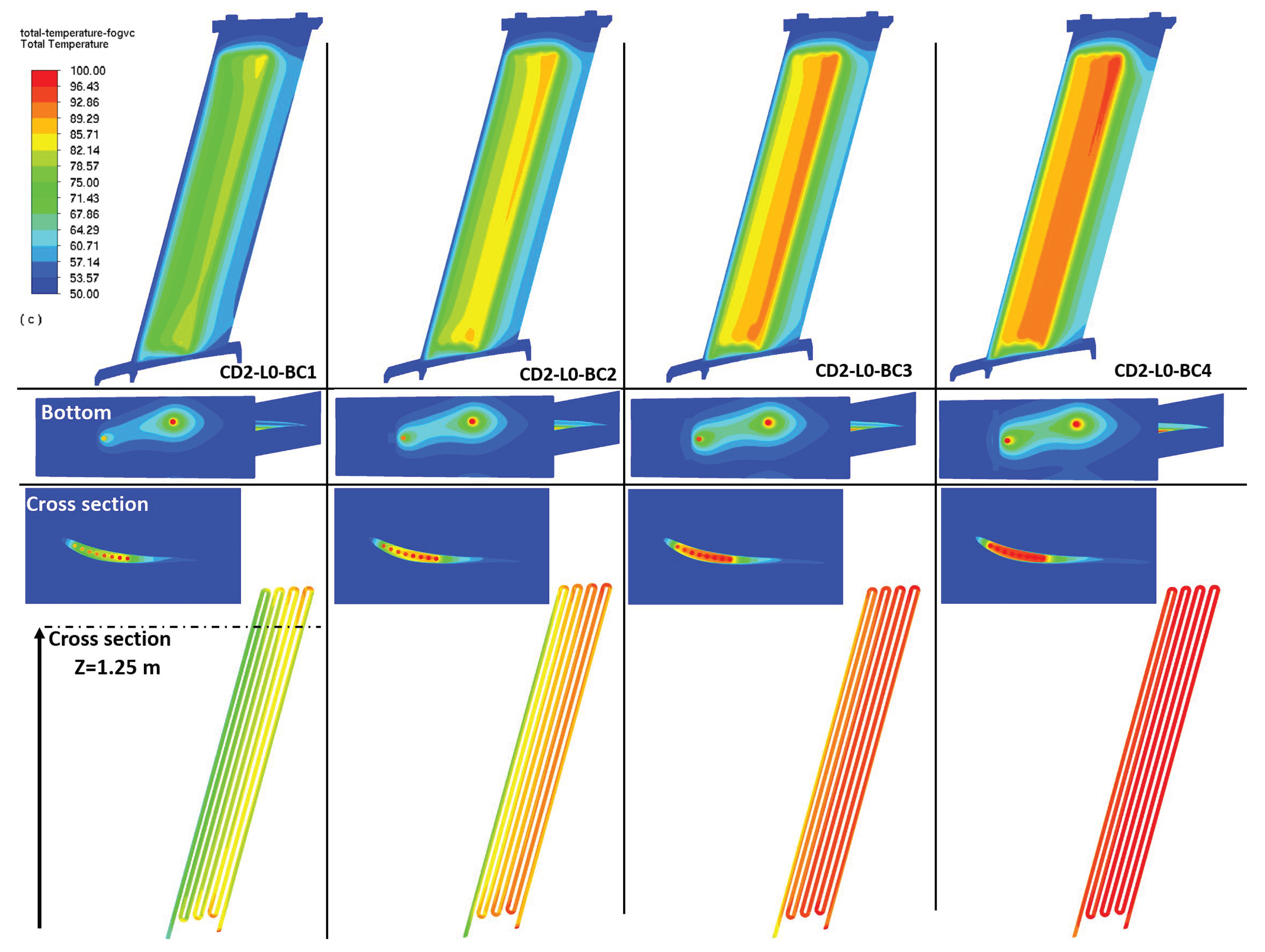
Figure 25.
Heat transfer coefficient distribution of L0 in CD1 and CD2 for the boundary condition BC4.
Figure 25.
Heat transfer coefficient distribution of L0 in CD1 and CD2 for the boundary condition BC4.
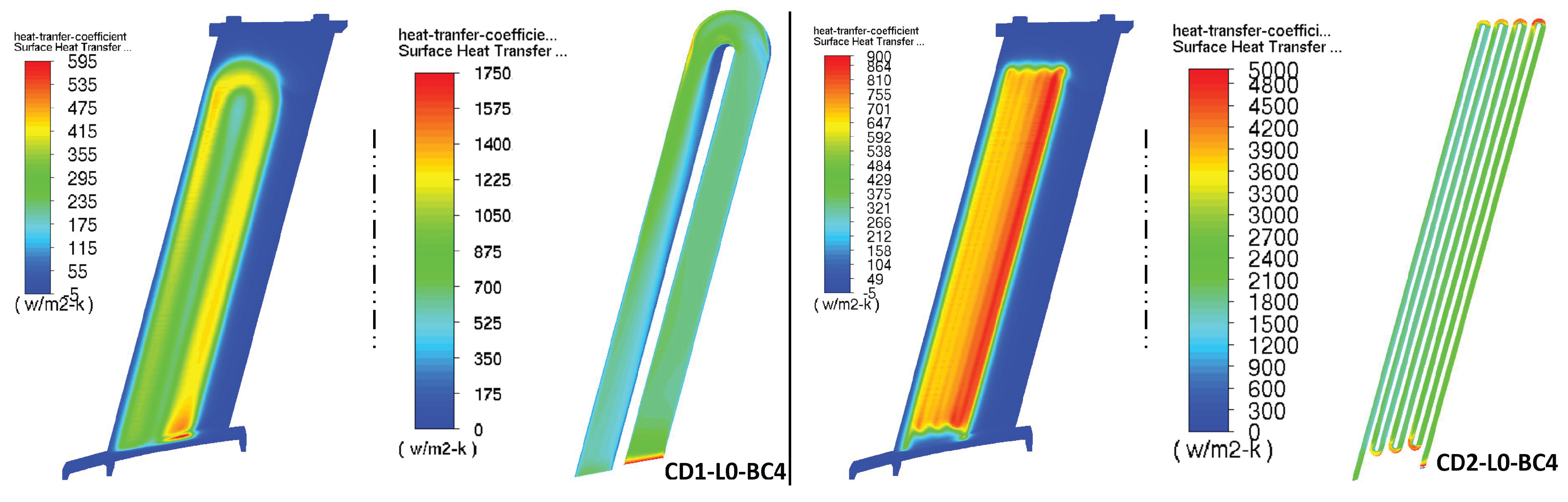
Figure 26.
Total velocity distribution of L0(O-M-A) in CD1 for the boundary condition BC1.
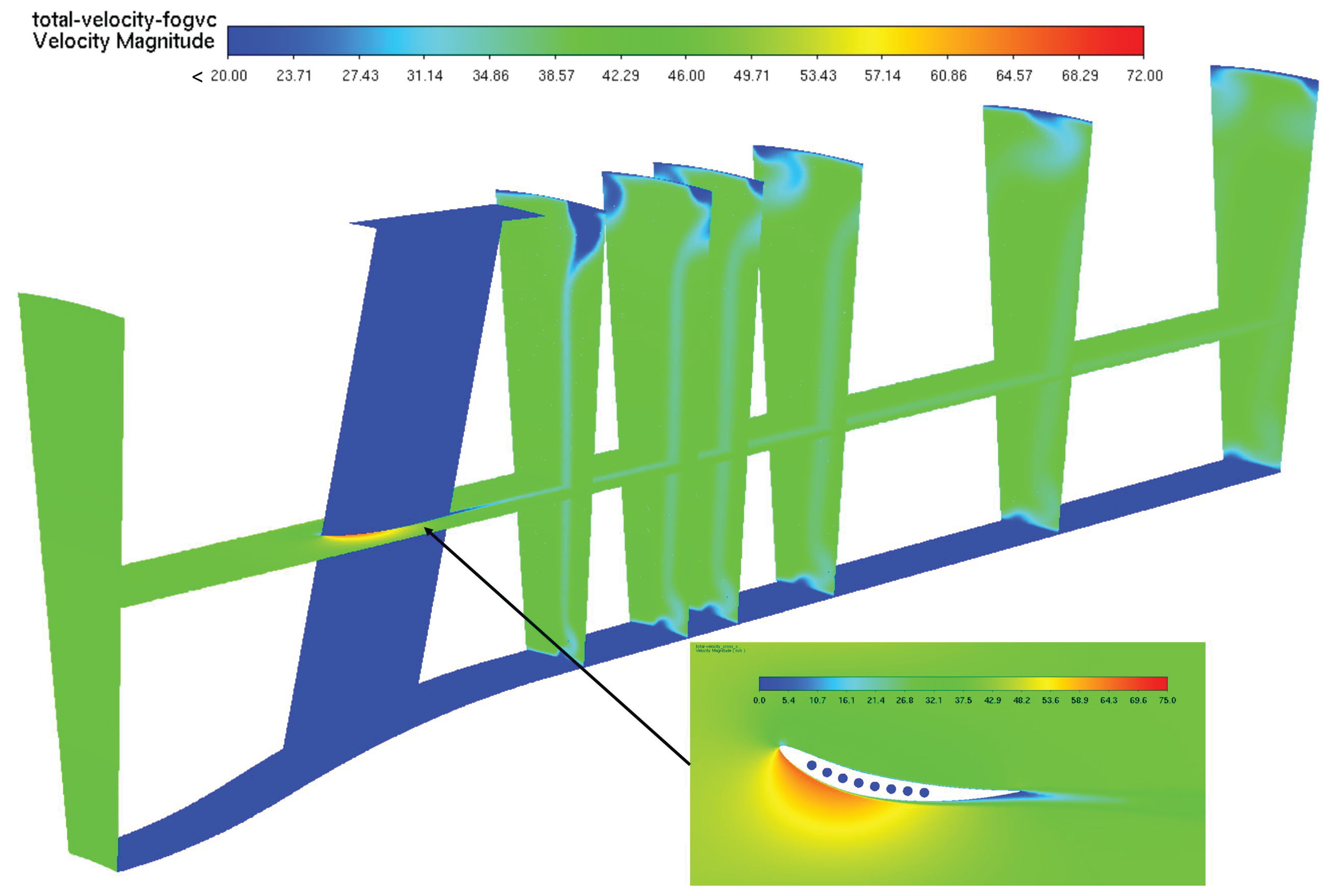
Figure 27.
Temperature distribution of CD1 at level L1 (O-M) using ANSYS Fluent™ for the boundary conditions BC5-BC12.
Figure 27.
Temperature distribution of CD1 at level L1 (O-M) using ANSYS Fluent™ for the boundary conditions BC5-BC12.
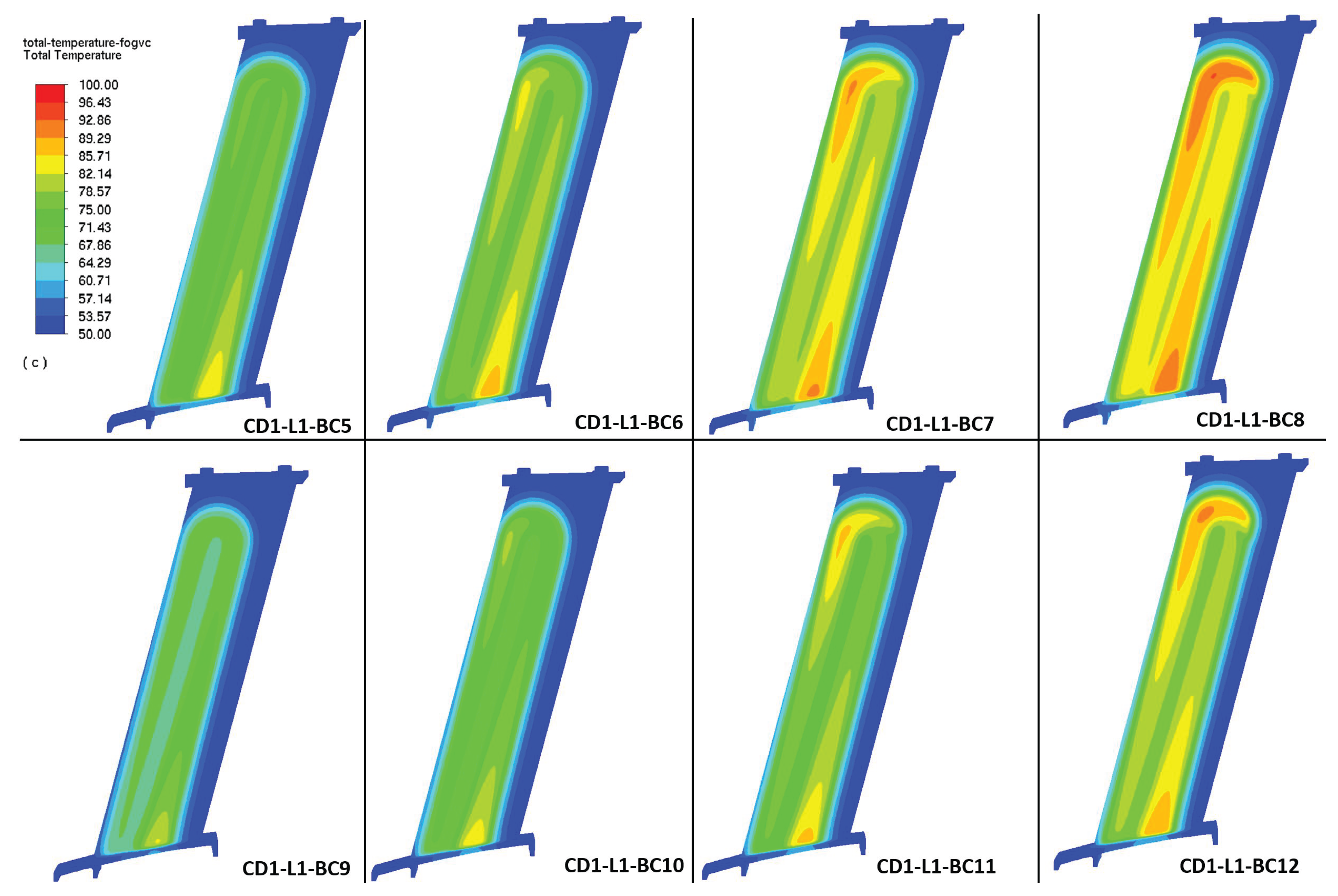
Figure 28.
Temperature distribution of CD1 at level L1 (O-M) using ANSYS Mechanical™ for the boundary conditions BC9-BC12.
Figure 28.
Temperature distribution of CD1 at level L1 (O-M) using ANSYS Mechanical™ for the boundary conditions BC9-BC12.
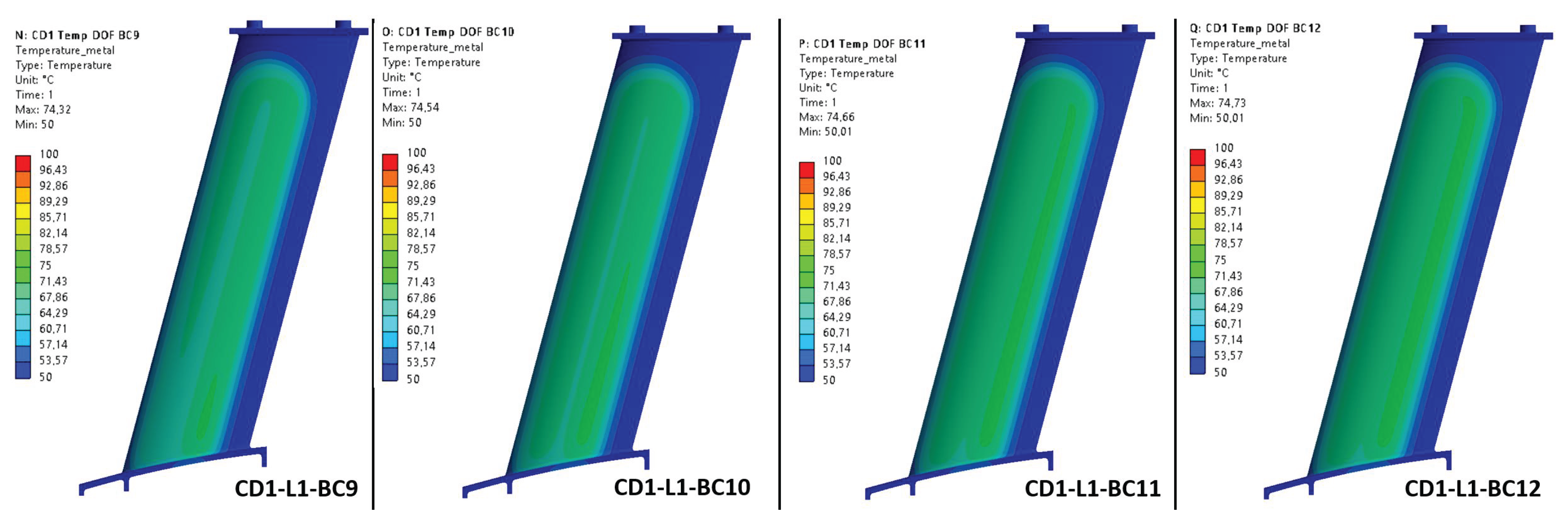
Figure 29.
Temperature distribution of CD2 at level L1 (O-M) using ANSYS Fluent™ for the boundary conditions BC9-BC12.
Figure 29.
Temperature distribution of CD2 at level L1 (O-M) using ANSYS Fluent™ for the boundary conditions BC9-BC12.
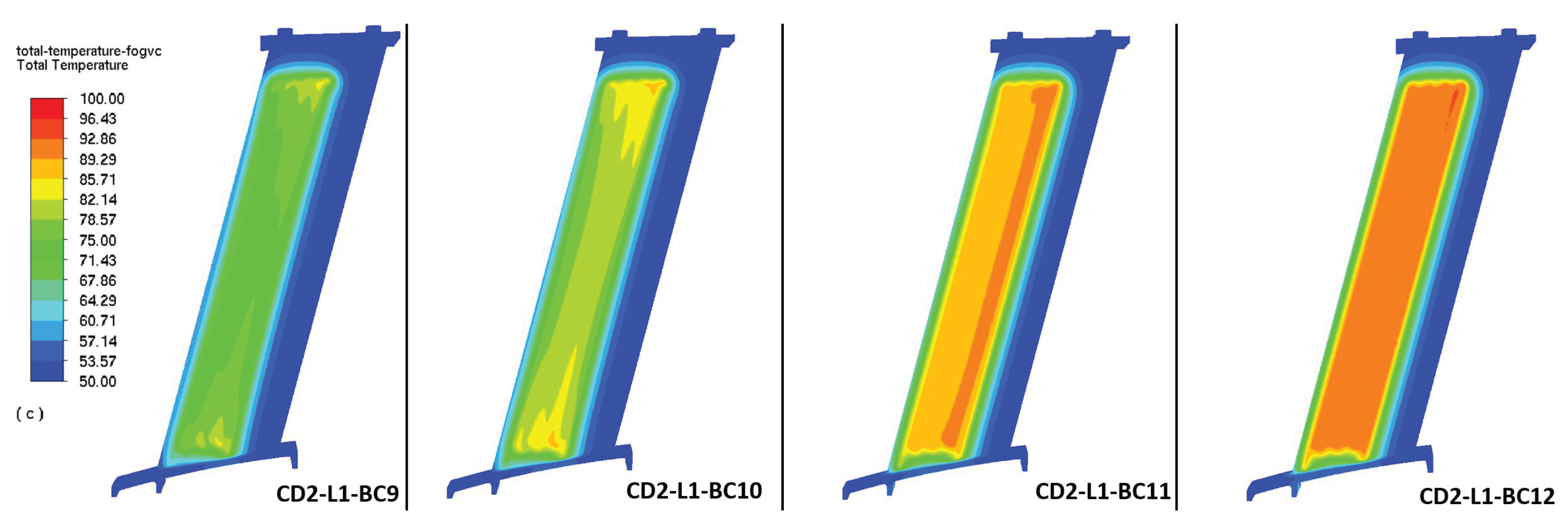
Figure 30.
Temperature distribution of CD2 at level L1 (O-M) using ANSYS Mechanical™ for the boundary conditions BC9-BC12.
Figure 30.
Temperature distribution of CD2 at level L1 (O-M) using ANSYS Mechanical™ for the boundary conditions BC9-BC12.
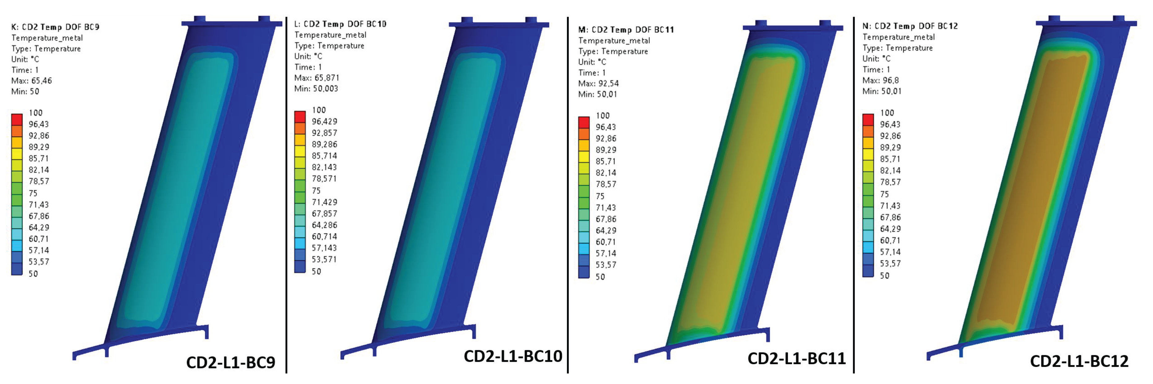
Figure 31.
Temperature distribution of CD1 at level L2 (O) using ANSYS Fluent™ for the boundary conditions BC9-BC12.
Figure 31.
Temperature distribution of CD1 at level L2 (O) using ANSYS Fluent™ for the boundary conditions BC9-BC12.
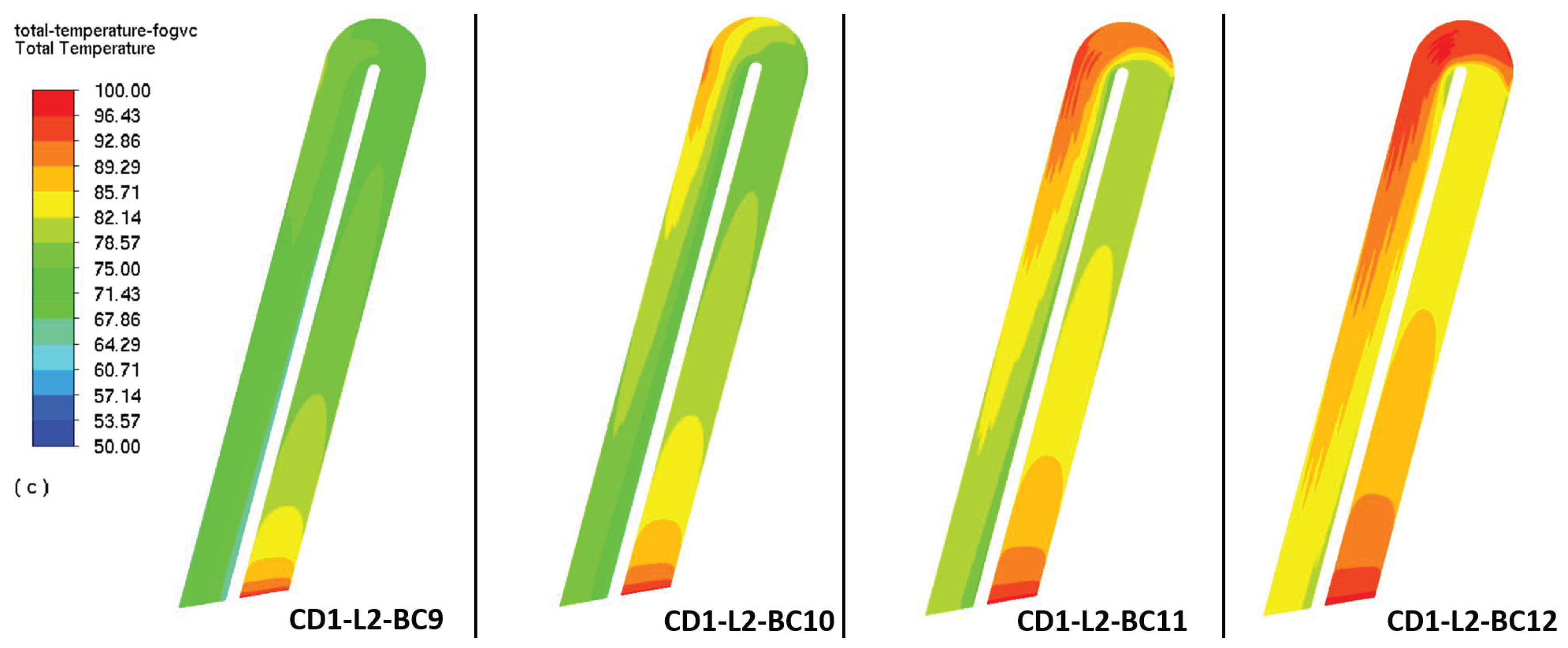
Table 1.
Overview of the boundary conditions for the air and oil domain, depending on the simplifications level. The sub-table on the left is defined for level 0 (L0) meanwhile the sub-table on the right for the levels 1, 2 and 3 (L1, L2 and L3).
Table 1.
Overview of the boundary conditions for the air and oil domain, depending on the simplifications level. The sub-table on the left is defined for level 0 (L0) meanwhile the sub-table on the right for the levels 1, 2 and 3 (L1, L2 and L3).
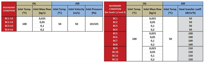
Table 2.
NTU method: heat capacity rates of oil, , air, , and associated heat capacity ratios, , for CD1 and CD2, using a of .
Table 2.
NTU method: heat capacity rates of oil, , air, , and associated heat capacity ratios, , for CD1 and CD2, using a of .
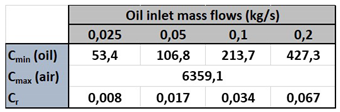
Table 3.
Proposal of dissipation areas by the analytical calculations for CD1 and CD2 and associated increases of the dissipated heat rates in the FOGVC.
Table 3.
Proposal of dissipation areas by the analytical calculations for CD1 and CD2 and associated increases of the dissipated heat rates in the FOGVC.
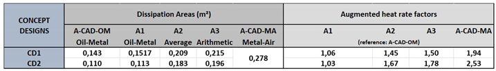
Table 5.
Number of finite volume elements used in the mesh refinements of the mesh study for CD1 and CD2.
Table 5.
Number of finite volume elements used in the mesh refinements of the mesh study for CD1 and CD2.
| Mesh refinement | O-Oil Domain [·10] | M-Metal Domain [·10] | ||||
|---|---|---|---|---|---|---|
| C-Coarse | 5.3 | 3.6 | ||||
| F-Fine | 10.4 | 4.9 | ||||
| UF-Ultra fine | 19.8 | 7.6 | ||||
Table 6.
Results of the mesh study of CD1 and CD2
| CD-1 | Max. | CD-2 | Max. | |||||
|---|---|---|---|---|---|---|---|---|
| Diff. | Diff. | |||||||
| Variables | C | F | UF | [%] | C | C | UF | [%] |
| Pressure drop (Pa) | 3085 | 3113 | 3124 | 1.2 | 110127 | 109993 | 109681 | < 0.5 |
| Outlet velocity (m/s) | 0.649 | 0.648 | 0.648 | < 0.1 | 2.772 | 2.771 | 2.767 | 0.1 |
| Lat. heat transfer (W) | -414.97 | -414.94 | -414.89 | < 0.1 | -448.17 | -448.15 | -448.2 | < 0.1 |
| Outlet temperature (K) | 371.2 | 371.2 | 371.2 | < 0.1 | 371.1 | 371.1 | 371.0 | < 0.1 |
Disclaimer/Publisher’s Note: The statements, opinions and data contained in all publications are solely those of the individual author(s) and contributor(s) and not of MDPI and/or the editor(s). MDPI and/or the editor(s) disclaim responsibility for any injury to people or property resulting from any ideas, methods, instructions or products referred to in the content. |
© 2025 by the authors. Licensee MDPI, Basel, Switzerland. This article is an open access article distributed under the terms and conditions of the Creative Commons Attribution (CC BY) license (https://creativecommons.org/licenses/by/4.0/).
Copyright: This open access article is published under a Creative Commons CC BY 4.0 license, which permit the free download, distribution, and reuse, provided that the author and preprint are cited in any reuse.


