
Submitted:
15 July 2025
Posted:
16 July 2025
You are already at the latest version
Abstract
The Solar System is analysed in the framework of the Complete Relativity theory (by the same author). While the main focus is on the Solar System, hypotheses are presented (and tested) on the origin and evolution of planetary systems in general, but also on the evolution of galaxies and the whole observable universe. The analysis confirms the postulates and hypotheses of the main theory and the hypotheses presented here with a significant degree of confidence. Some of these are: relativity in the invariance of physical laws (i.e., existence of discrete vertical energy levels, where each discrete scale of energy effectively represents a universe, associated with the universal running of couplings) and complete relativity in everything, Solar System is a large scale (inflated, in some interpretations) quantum system (Carbon/Beryllium isotope equivalent) with a nucleus in a partially condensed state and components localized in various horizontally and vertically excited states, life is everywhere (e.g., Earth is a particle, but also a living being), although the presence of extroverted complex forms on the surfaces of celestial bodies is generally very limited in time, anthropogenic climate change is only a part of a major mass extinction event (although humanity definitely has a role, the sense of control is an illusion), major extinction events on a surface of a planet are relative extinctions, may be a regular part of transformation and migration of life (not necessarily complex living individuals) below the surface in the process of a planetary equivalent of embryonic neurogenesis.
Keywords:
solar system
; complete relativity
; nature
; mechanics
1. Introduction
According to Complete Relativity[1] (CR), everything is relative. Any apparent absolutism (notably scale invariance of dimensional constants, absolute elementariness or invariance to time) is an illusion stemming from limits imposed by, or imposed on, polarized observers. It is also a result of excessive appliance of reductionism (abuse of the Occam’s razor) to naturally holistic reality, which inevitably leads to misinterpretation of phenomena (another illusion). A deeper understanding of observables, thus, requires a holistic approach. The CR theory has been constructed in order to provide a framework that could be used for deeper understanding of fundamentals of reality, regardless of scale. The results of analyses done here are a vivid testament of its power.
Here, for example, I hypothesize, and provide solid evidence, that the Solar System is a localized large scale quantum system. In different interpretations, it is consistent with a relative 10C (10-Carbon isotope), or a 10Be (10-Beryllium isotope) atom equivalent, or a localized superposition of such isotopes in a relatively special state (regarding scaled pressure/temperature). The analyses done provide evidence not only for the relative equivalence of large (U1) scale systems with standard (U0) scale systems, but for the relativity of scale invariance of physical laws (conventionally assumed to be absolutely scale invariant).
Note that an 10C isotope is unstable on standard (U0) scale, with a half-life of ∼19.3 seconds. Its apparent relative stability on U1 scale (from our perspective) is mainly a result of time dilation that exists between scales, but also due to relativistic energy on this scale.
The Un scales here represent discrete vertical energy levels and are defined in CR. U0 corresponds to the scale of standard atoms, U1 is the scale of planetary systems, while U−1 is the scale that is orders of magnitude smaller than U0 and represents the scale of particles (gravitons) forming space associated with U1 particles (standard photons also belong to U−1 scale). A different scale generally corresponds to different rest masses, but also to different radii of localized particles.
I also hypothesize that the formation of planetary systems in general starts with the inflation of gravitons from the scale of standard atoms (or even lower scale equivalents), likely in the events of annihilation at relative event horizons of larger scale.
Gravitons here should not be confused with the hypothesized gravitons in theories based on Quantum Mechanics (QM). In CR, a graviton is a generalized term, representing a fundamental form of energy, but its nature is not fundamental. It thus represents a form of energy that can evolve into all the different kinds of particles. It can be more or less polarized (e.g., electrically charged), it can be elementary (relative to particular scale) but not absolutely, and it can be relatively massless (but not absolutely). Usually (by default), it is considered as a carrier of general force, which, in CR, is a superposition of gravitational and electro-magnetic force, where usually one force dominates (with dominance generally depending on scale).
Gravitons, as defined in CR, should exist at different scales. But these scales are probably not limited to the hypothesized major discrete vertical energy levels. Rather, a graviton (with more or less evolved nature) of appropriate scale is probably coupled with any emergent phenomenon, which represents something more than the sum of its parts. In fact, this coupling is probably required for the emergence, albeit the strength, frequency and duration of couplings can vary. Effectively, this suggests that every emergent physical phenomenon represents a universe of its own, although many such universes can represent relative clones of each other. By the postulates of CR, however, no two universes (e.g., two electrons) are absolutely the same. However, observers are inherently limited and one may not be able to distinguish between individuals of certain species.
Some might argue that the nature itself is limited by the Heisenberg uncertainty principle. However, it should be clear, that, by the postulates of CR, such principles themselves must be relative.
Since gravitons are fundamental (only their properties/couplings evolve with scale), and, based on my research, probably should also be interpreted as carriers of consciousness, consciousness itself is fundamental, and all these couplings are relatively conscious of the local reality, proportionally to the strength/localization of coupling.
Obviously, one should be familiar with the tenets of CR in order to fully understand this paper. Some terms used in the paper are described in greater detail in CR, but may lack description here. Apart from the "graviton", some other terms used may be defined differently in CR than they are conventionally defined. Although some of this should be intuitively clear, the reader is advised to consult CR for definitions of these terms (e.g., gravitational maxima, gravitons, vertical energy levels) in order to avoid confusion.
I propose that, in the process of inflation of gravitons associated with planetary systems, the electro-magnetic component of the general force is exchanged with the neutral gravitational component, resulting in the dominance of gravity over electro-magnetism at this scale. However, I also propose that such exchange may be natural on standard scale - particles could be cycling between polarized and neutral states. In case of U1 systems, the system likely starts inflation from U0 electro-magnetic with gravitation becoming dominant afterwards. At the end of a lifecycle gravitons may collapse again (deflate) to U0 again, now exchanging gravity for electromagnetic force. It is the opposite for U0 systems inflating from U−1 scale - inflation starts gravitational but ends up in electro-magnetic equilibrium.
Note, however, that this does not imply that dominant forms of energy on particular scale are absolutely dominant. Proper conditions (i.e., at certain properly scaled temperature/pressure) can ensure stability of non-dominant forms.
In any case, obviously, the hypothesized equivalence between the Solar System (or any planetary system, in general) and an atom should be taken relative. Note also that various interpretations will be presented and explored here, some of which may be mutually incompatible, while some may be simultaneously true.
Implications of CR on the understanding of nature are large and particularly affect the understanding of life. Existence of vertical energy levels is required for conservation of relativity but one consequence is relativization of components of living beings (e.g., living tissue, blood, etc.) between scales - they operate on different timescales and generally have different composition. In example, standard blood (blood composed of U0 scale atoms), scaled to U1 will not be the same substance simply containing zillion extra standard blood cells, rather, to an U0 scale observer (e.g., human) it will appear much different. Indeed, what I will consider the blood equivalent of a planet is commonly interpreted as magma. Thus, the planets (particles) can be living beings and here I will analyse Earth not only as a particle but as an evolving/developing living being.
2. Constants
Table 1 shows commonly used constants in the paper.
The values of planetary constants are taken from NASA Planetary Fact Sheets [2], year 2020.

Table 1.
Commonly used constants.
| Description | Constant | Value |
|---|---|---|
| Neptune mass on scale | 1.02413 × kg | |
| Neptune equivalent mass on scale (localized in e eigenstate) | 9.109182827 × kg | |
| Localized Neptune orbital velocity on scale | 5430 m/s | |
| Localized Neptune spin velocity on scale | / (16.11 × 60 × 60) = 2668 m/s | |
| Localized Neptune radius on scale | 24622000 m | |
| Localized Neptune equivalent radius on scale | ( / ) × = ( 24622000 m / 4495060000000 m ) × 70 × m = 3.834298096 × m | |
| Solar System charge radius = .Neptune.orbital.radius | 4495060000000 m | |
| Sun mass | 1.988500 × kg | |
| Sun radius | 695735 km = 695735000 m | |
| Earth mass | 5.9723 × kg | |
| Standard Carbon-12 atom mass | 1.992646547 × g = 1.992646547 × kg | |
| Standard Carbon-12 charge radius = Carbon-10 charge radius (covalent) | 70 pm = 70 × m | |
| Standard Carbon-10 nucleus charge radius | 2.708 × m | |
| Standard Carbon-10 nucleus mass | 10.016853 u = 1.663337576 × kg | |
| Standard speed of light | c = | 2.99792458 × m/s |
| Standard electron mass | 9.10938356 × kg |
3. Definitions
Definitions of terms and expressions that may be used in the paper. Note that at least some of these may also have conventional definitions which are different, and at least some should be understood as hypotheses.
3.1. Weak and Strong Evolution
Rates of evolution or flows of energy cannot be absolutely constant. Energy on one scale is generally entangled with energy on other scales (which, in some cases, can be interpreted as simultaneous existence on multiple scales) and time dilation exists between these scales. A particular state on one scale (characterized by relatively discrete jumps between energy levels) can be interpreted as the attractor for the other scale (characterized by continuous transition between points of inter-scalar equilibria). With attraction generally being exponentially correlated with distance (in space/time) one can assume that between two equilibria evolution proceeds at a relatively constant rate but near the points of equilibria the rate grows and decays exponentially.
A period of relatively constant rate of evolution may be referred to as [a period of] weak evolution, while a period of accelerated evolution may be referred to as [a period of] strong evolution.
Speed of motion trough time is generally different between scales (although, in some interpretations, the metric may be scaled). On one scale, transition between states can be relatively instantaneous, on the other continuous. In case of entangled scales, this implies that the measurement of the continuous change of energy can be used to determine when will the discrete jump on the other scale occur. In example, if the changes are decelerating, the discrete jump on the larger scale may have occurred recently. On the other hand, if the rate of change is accelerated, the discrete jump is likely [relatively] imminent. Generally, discrete jumps on larger scale will be synchronized with cataclysmic changes on the smaller scale. This can be interpreted as non-linear attraction of energy towards eigenvalues. Thus, evolution of energy is generally characterized by the periods of weak evolution (when the rate is relatively constant - oscillating about some mean value) and periods of strong evolution (when the rate is accelerating/decelerating) near the ends/beginnings of transition. This behaviour should be typical for all changes in energy levels, only the magnitude of changes varies.
3.2. Primary Atom Radius
Generally, radius of an atom is assumed to be equal to the radius of its outermost electron orbit.
However, other particles can be bound to atomic nuclei. Here, it is hypothesized that neutrinos and anti-neutrinos are commonly bound to nuclei, generally occupying separate energy levels but may also be bound with other particles (e.g., forming electron-neutrino pairs).
Primary radius of the atom is then equal to the orbital radius of its outermost primary component. At minimum, it is equal to the general radius of the atom (outermost electron orbit). However, in equilibrium - with all primary neutrinos present, it may be over twice that radius.
Here, a bound particle is considered primary if it is a component of the system equilibrium state (this is further discussed in chapter 6. Initial structure hypothesis).
One could argue that neutrinos and anti-neutrinos, being neutral, cannot be bound to atomic nuclei because electro-magnetic force is the dominant force and gravity is weak. However, as it will be shown later, planetary systems are relative equivalents of atoms and, in these, equivalents of lower mass particles commonly orbit the nuclei. If the formation of planetary systems starts with inflation of energetic atoms in extreme conditions (e.g., through annihilation at event horizons), then these lower mass particles probably have existed in the atoms as well. However, as electro-magnetic force is, with inflation, effectively exchanged for gravitational force, it is possible that these lower mass particles have some charge on standard scale. They could be then interpreted as charged neutrinos - since they do appear to have neutrino-like masses, but any significant charge is unlikely. After all, zero total charge does not prevent neutrons to couple with protons.
It is however, also questionable, whether any of the charged particles are charged all the time even on the standard (U0) scale. Exchange of the electro-magnetic component of general force for gravity could periodically occur even if usually for brief moments (correlated with time-energy uncertainty), and what happens at [critically] low temperatures where properties of space (e.g., magnetic permeability and vacuum permittivity) are effectively changing? Are all heavy bosons in general electrically neutral? Note that particles such as W bosons are never detected directly - their charges are thus purely theoretical, based on the assumption of charge conservation. Charge may not be [completely] conserved in bosons, rather exchanged for gravity. Note that this can also explain pairing of like charges (not necessarily limited to Cooper electron pairs). The exchange can also explain bosenovas, in which case, these do not only resemble supernovas - they are small scale supernovas.
3.3. MAU
MAU or Mars relative Astronomical Unit is a unit of distance. 1 MAU is equal to the distance of the outermost positive charge from the atom nucleus centre.
On the scale of the Solar System (U1 scale), 1 MAU is equal to the distance of planet Mars (hypothesized equivalent of positive charge) from the Sun.
It is assumed that in the equivalent system on standard (U0) scale Mars would be positively charged. On U1 where, due to dominance of gravity, it may be difficult to associate specific electric charge to planets, charge may be correlated with other properties of a body (e.g., difference in magnetic spin between the planets).
Note also that in anti-matter systems 1 MAU would be equal to the distance of the outermost negative charge from the nucleus.
3.4. Nuclear decay
Quantum Mechanics offers a solid mathematical description of nuclear decay, however, it doesn’t offer a satisfying physical interpretation of the process. The models described here, however, provide exactly that - a more detailed picture of its mechanics and nature.
Weak nuclear decay transforms a neutron into a proton, or vice versa. If these are parts of an atom, this is nuclear transmutation - transformation of one atom of an element into an atom of another element. Another type of nuclear transmutation is the -decay.
Per the hypothesis here, neutrinos and anti-neutrinos can be, like electrons, bound to atomic nuclei occupying appropriate energy levels (and, as other fermions, may be grouped into pairs). In equilibrium, the number of bound electron (e) neutrinos and electron anti-neutrinos within the [primary] radius of the atom corresponds to the number of protons and neutrons, respectively. These are, together with nuclei and electrons, primary components of the atom. Decay process, in one interpretation, involves annihilation of neutrinos and anti-neutrinos and stability of elements will depend on their number, ratio and excitation.
Energy levels are scale relative and sensitivity to particular force is scale relative. A particle has different energy density/radius depending whether it is in a localized or non-localized wave form (or, depending how much it is localized or non-localized). Quantum tunnelling effects are then possible in delocalized forms. Particles generally periodically oscillate between localized and delocalized forms. Nuclear decay probably occurs with the destabilization of this cycling. When the period of time in a delocalized state is increased, the expanding wave may reach the nuclear barrier at the point of localization where it can then overcome the attraction of the strong nuclear force even in the localized form. Multiple [types of] barriers exist. Barriers closer to the nucleus are occupied by neutrons, while the outer ones are occupied by primary neutrinos. Generally, neutral particles of one scale are localizing with the interaction with charged particles of another scale, and vice versa. Equally charged particles can, for example, tunnel through each other in wave form - it is the neutral photon emitted with the accelerated charge that interacts with other charges. The tunnelling is then more likely to occur the lower is the acceleration (otherwise, the absorption of photons results in what can be interpreted as effective interaction between charges themselves). Different interpretation for decay, are, however, possible - depending which particle is actually tunnelling.
Stability requires cycling resonance between bound particles, with the time to de-synchronization, on average, equal to the half-life period of the element. Once an atom decays, at the same time, the cycling of the neighbouring atom [of the same isotopic species as the original element that decayed] is reset (brought into resonance) with the absorption of information (energy of particular scale) emitted with the decay. Thus, the lifetime of a neighbour is extended by the half-life period [on average], explaining the peculiar nature of the decay process. Note that the non-absolute cycling synchronization is the key here (along with the finite information transfer speed). If all atoms would decay exactly at the same absolute instant, there would be no atoms left for the cycling reset.
3.4.1. -Decay
In this process, an unstable nucleus decays to another element with the emission of an particle, composed of 2 protons and 2 neutrons (a Helium nucleus).
The instability occurs when the proton waveform [expansion] reaches a neutron barrier. Usually, however, 2 neutrons occupy a single barrier and 2 protons are required for destabilization (the Coulomb potential of a single proton is insufficient to overcome the barrier). With the localization of protons at this barrier, the Coulomb repulsion between the 2 protons and the nucleus prevails and the 4 particles are ejected from the nucleus as an -particle.
3.4.2. Decay
This is a transformation of a neutron to a proton, with emission of excess energy:
Here, in one interpretation, waveform of a down quark at the time of decoherence during localization/delocalization cycling forms a superposition of 2/3 e+ and 1 e− charge flavours, which could be interpreted as a superposition of up quark and electron flavours but with a larger (more massive) neutral flavour components (mass). The delocalization thus produces one up quark and one electron waveform. If the electron waveform reaches the anti-neutrino occupied barrier before localization, it localizes there, coupling temporarily with the anti-neutrino (which can be interpreted as a new particle, a W boson) - at which point the strong attraction has been overcome, and the two are ejected together from the nucleus, while the up quark is, with the recoil in the opposite direction, bound to the nucleus.
Note that, while the localization of the charge at the neutral barrier is unstable, localization of a neutrino at the charge closer to the nucleus may be correlated with increased stability. Note also that a delocalizing graviton (whether it is neutral or polarized) will leave behind real mass, which can be recycled (coupled to the graviton again) with the localization to the same location. This kind of cycling is then, in equilibrium, a closed system.
Note that both, charges and neutrinos are undifferentiated/naked in a free wave form. Mass differentiation (speciation) occurs with the localization (coupling to real mass). It is thus technically incorrect to state that a down quark is a superposition of an up quark and an electron. More appropriate is to say that the 1/3 e− flavour evolves from the mixing/resonance of 2/3 e+ and 1 e− charge waveforms (flavours), while the down quark particle evolves from the coupling of that flavour with the amount of real mass corresponding to the down quark mass eigenstate. However, in contexts where particular flavour (e.g., 1/3 e−) generally evolves into one particular species (e.g., down quark), it can be considered as a precursor to that species and may be referred to as a waveform of that species.
In another interpretation, the de-synchronization is big enough to allow for bound non-primary e neutrino and bound primary e anti-neutrino to annihilate and produce, depending on energy, either an electron/positron (e−/e+) pair, or up/anti-up quark pair:
Here, an intermediate step in the form of a boson (e.g., Z) is implied.
In case of electron/positron production, positron further partially annihilates with the down quark (here, both are composite particles), producing neutrino/anti-neutrino pair and an up quark:
Is partial annihilation here the appropriate term/process? It is possible that the positron and down quark flavours [along with a neutral component] combine into superposition when they are delocalized during regular cycling, and this superposition evolves then into an up quark, while the other neutral component evolves into an anti-neutrino (neutrino is not created).
Neutrino bounds to the atom [as a primary component], while anti-neutrino and electron localize into a spin paired state (boson), before decoherence and separate ejection:
Note that, per QM, lepton number has to be conserved in particle interactions and the neutrino in step (2) cannot be created (at least not without an additional anti-lepton). If this is indeed not violated in reality and the neutrino is not created here, it is possible that the space reserved for a primary neutrino (with the creation of the proton) is filled with a bound non-primary neutrino. Note also that a large scale gravitational disturbance (temporary change in properties of space) is, in effect, the disturbance of both uncoupled and bound static [graviton] neutrinos (components of local space coupled to the atom) and these can then affect the mass and rate of creation of W bosons, allowing for decay rates of elements to significantly deviate from the average (per CR, they should generally oscillate about a mean value), even if temporarily. Note that comparison of experiments and discrepancies[3] (between obtained W boson masses and QM standard model prediction) clearly show that oscillation/deviation is real.
In case of up/anti-up quark production in the first step, the up quark is absorbed, while anti-up quark pairs with the down quark before transformation and ejection:
Note that a decay of W− into an electron and anti-neutrino even when it is created from anti-up and down quarks would suggest that charge in electron is a composite of 1/3 and 2/3 charge quanta. In the decay of a proton to neutron through electron capture, electron could then [inverse] decay to u− and d− by pairing with an anti-neutrino (inflating to W− boson), u− would annihilate with u+, leaving 2 down and 1 up quark, forming a neutron.
Outside of the atom, the transformed pair (W boson) is unstable (short-lived), except in extreme conditions.
Note that, in this case, to conserve equilibrium conditions, one of bound non-primary e neutrinos must reduce its orbit to become a primary component.
decay is the effective transformation of a down quark to an up quark of the atom nucleus.
Boson Mass
According to the Standard Model of particle physics, the rest mass of the W boson is more than 80 times higher than neutron mass and orders of magnitude higher than that of down and up quarks.
Thus, the production of a W boson is apparently a violation of energy conservation. In QM perturbation theory this is solved with the time-energy uncertainty principle which allows production of such particles (borrowing vacuum energy) providing they decay quickly (lifetime of a W boson is ∼10−25 seconds).
Note that this is compatible with CR, assuming production and energy borrowing are interpreted as inflation of energy from a lower (unobservable) vertical energy level into a higher vertical energy level. Since the lower level is unobservable, energy conservation is relatively violated. Absolutely, however, it is not.
However, mass of the boson is also considered variable with probability of deviation from the rest mass decreasing fast with the amount of deviation, thus, making probability of beta decay proportional to the probability of creation of a low mass W boson (∼1 MeV).
In reality, there is no violation of energy conservation (in modern QM interpretations there is no violation either, however, the solution is much worse - the particles are declared virtual and are commonly assumed not to exist in reality although they are mathematically required intermediates) and the mass of a W boson is, in fact, a result of conservation of energy due to momentum - energy coupling (note that, per CR postulates, even rest mass has a momentum, albeit relatively confined), where one component of the angular momentum is exchanged for the other. In this case, the angular momentum of a particle orbiting the nucleus is collapsed [localized] to a spin momentum, where radius has been effectively exchanged for energy [inflation].
How Much Are Produced W Bosons Charged?
In QM, it is assumed that charge is conserved with the creation of a W boson in case of coupling of a charged particle with a neutrino/anti-neutrino. But is that the case?
In CR, transition between major vertical energy levels generally involves exchange between polarized (e.g., electro-magnetic) and neutral (e.g., gravitational) potential. Does the same exchange happen in case of smaller or minor vertical energy levels? This may depend on the mechanism involved (i.e., whether annihilation is involved), but it is possible that with the W boson creation (mass inflation) electro-magnetic potential is exchanged for gravitational and as W decays it is converted back to electro-magnetic (therefore, increasing Coulomb repulsion, enabling ejection). Thus, although W boson here is theoretically charged in QM, and charge is conserved between initial and final state of the system, in reality it may not be conserved in the boson itself (unless the inflated mass is indeed extremely low compared to the rest mass).
Probability of beta decay is then proportional to the conservation of charge in the inflated W boson (more massive W boson wouldn’t be charged enough to escape).
Destabilization of cycling correlated with nuclear decay can then also be interpreted as spatial/temporal asymmetry in exchange between neutral (gravitationally strong) and polarized (electric) potential.
In any case, stability must be relative and coupling of charged particles with neutrinos can be stable, although this may require relatively extreme conditions (e.g., Bose-Einstein condensates or time-dilated scales/environments).
3.4.3. Decay
Transformation of a proton to a neutron, with emission of excess energy:
Here, in one interpretation, the up quark at the time of decoherence during cycling forms a superposition of 1/3 e− and 1 e+ charge flavours. This produces one down quark and one positron waveforms. If the positron waveform reaches the neutrino occupied barrier before localization, it localizes there, coupling temporarily with the neutrino (into a W boson) - at which point the Coulomb repulsion overcomes the strong attraction, and the two are ejected together from the nucleus, while the down quark is, with the recoil in the opposite direction, bound to the nucleus.
Note that this type of decay generally occurs in proton-rich nuclei. A single isolated proton does not have enough energy to transform into a neutron (convert an up quark into a down quark). In other words, there is no enough energy to inflate the neutral graviton component enough so that it could settle into a stable down quark mass eigenstate.
In another interpretation, bound primary e neutrino and bound non-primary e anti-neutrino annihilate to produce either an electron/positron (e−/e+) pair, or down/anti-down quark pair:
In case of electron/positron production, electron further partially annihilates with the up quark (here, both are composite particles), producing neutrino/anti-neutrino pair and a down quark:
Similar to the case of decay, the anti-neutrino here may not be produced unless one additional particle on the left side of the equation is involved (due to violation of lepton number conservation). Note that this additional particle can be one of the primary anti-neutrinos that usually occupy barriers between positive and negative charges.
The anti-neutrino bounds to the atom [as a primary component], while neutrino and positron are ejected in a spin paired state (boson), before separating again:
In case of down/anti-down quark production in the first step, the down quark is absorbed, while anti-down quark pairs with the up quark before transformation and ejection:
Note that, in this case, to conserve equilibrium conditions, one of bound non-primary e anti-neutrinos must reduce its orbit to become a primary component.
decay is the effective transformation of an up quark to a down quark of the atom nucleus.
3.4.4. Inverse Decay
Transformation of a proton to a neutron by electron anti-neutrino scattering:
In one interpretation, decoherence of the up quark during cycling creates one 1/3 e− and one 1 e+ waveform. The anti-neutrino couples with the 1/3 e− flavour, inflating the neutral component of the coupling to the down quark rest mass eigenstate. The 1 e+ waveform evolves into a positron with the scattering and is ejected from the nucleus (may carry most of the excess anti-neutrino energy).
In another interpretation, this interaction may occur when the atom is not in equilibrium, more specifically - the number of bound e neutrinos is lower than the number of protons.
In this process, e anti-neutrino annihilates with a bound non-primary e neutrino, initiating a decay with electron/positron product:
Again, the anti-neutrino here may not be created unless an additional particle is involved.
However, since the number of bound primary e neutrinos was initially lower than the number of protons, now even the created neutrino is bound (as a non-primary component) rather than ejected with the positron:
3.4.5. Electron Capture
Transformation of a proton to a neutron by electron capture.
Electrons are separated from positive charges in the nucleus by barriers (relative event horizons). Electron capture occurs when high external pressure causes one of the innermost electrons of the atom to overcome the barrier (event horizon) - occupied by the corresponding anti-neutrino, and enter the nucleus. This results in partial annihilation with the up quark, proceeding further as decay:
The anti-neutrino bounds to the atom [again] as a primary component, while neutrino gets ejected:
Although not shown, intermediate steps here are possible (creation of W bosons). Note that the inclusion of the primary anti-neutrino here solves the problem of violation of the lepton number conservation. Thus, such primary particles may indeed be involved in other types and interpretations of decay where the potential violation occurs.
3.5. Spin Momentum
Spin momentum is an intrinsic property of gravitons, and it represents an self-orbital angular momentum in CR (rotation with spin radius greater than absolute 0). Excessive reductionism in modern science has made it a confusing concept, however, it should be clear that it is certainly associated with rotation in the mathematical formalism of modern physics, it is only the limitations of established theories that do not allow certain processes described in mathematical space (time) dimensions to have such interpretation in reality that would involve physical rotation.
The reason behind this is that modern science on average is more concerned with measurement and prediction of measured values, not with the accurate description of reality.
Although the two terms are highly correlated, difference, however, exists in the properties of spin and spin momentum. Spin momentum implies physical rotation on some scale (at least in CR), however, spin in mathematical formalism is a non-dimensional value, usually associated with symmetry of objects under rotation. For example, the photon has a spin of 1, implying that it is symmetric under rotation of 360∘, gravitational waves, on the other hand, need only to be rotated by 180∘ to look the same, so they (or associated gravitons) have a spin of 2 (360 / 180 = 2).
Gravitational waves travel as pulsating tidal bulges, compressing space in one direction, expanding it in another, so the cross-section of the wave has a form of the ellipse. An ellipse or an ellipsoid only needs to be rotated by 180∘ to look the same. An electro-magnetic wave is a combination (superposition) of an electric and an magnetic pulse which are perpendicular to each other, however, axial symmetry here requires a full rotation of the wave (360∘) because the pulsation relative to the electric and magnetic axes is not symmetric.
Electrons (or electron waves) have a spin value of 1/2, needing 720∘ for axial symmetry. This doesn’t imply anything physically non-intuitive, it just implies that the rotation is more complex (e.g., a superposition of two different angular momenta).
4. Elementary Particles and Interpretations Thereof
Elementary particles or waves, relative to a universe of a particular scale, are generally polarized.
Physical interpretation (manifestation) of polarization depends on environment, but any elementary particle can be interpreted as a more or less evolved graviton (as defined in CR).
Note that, in CR, elementary particles are not absolutely elementary, reference frames will exist where existence of constituent particles is apparent and real.
In case its electro-magnetic component is dominant, the particle is electrically polarized (charged) and represents a relative electric monopole.
However, electric component is generally a sum of multiple constituent charge quanta, typically 2 quanta of identical charge and 1 quantum of opposite (anti) charge, which are strongly entangled (there are no absolute monopoles). Spin momentum of charge is quantized, by a relative constant (ℏ) - a quantum of momentum, which is a consequence of harmonic oscillation of waveforms of energy in some reference frames (scales). Note that quantization is not absolute, a particle may exist in a superposition (generally linear combination) of base states and thus in reality can take any value in between. It is only upon localization (collapse of the wave form) that the choices may be narrowed to base values.
Of course, in reality there is no absolute isolation or absolute randomization. Thus, a superposition itself will be limited in values, although this limitation may not be observable from some reference frames. For example, consider a simple refrigerator magnet. It is composed of both mass and charge so it responds to multiple forces of different nature (or multiple components of general force). It may be oriented randomly by the wind, for example, but there will also exist a tendency for the alignment with the background magnetic field (e.g., Earth’s). Before a stronger magnetic field is applied (overpowering other forces), its alignment may be considered to be in superposition of two base states (e.g., up and down), but even in this state, some values will be more likely than others. However, the background forces fluctuate and oscillate so the resolvability of this affinity will depend on the scales of space and time associated with the observational momenta.
Collapse of the wave form is usually associated with measurement or manipulation, however, the act does not have to involve conscious observers. Generally, it involves thresholds in localization pressure. Once the form is collapsed, a particle may remain in that state for a long time. Now, if measurements are done relatively frequently and axes of measurement (quantization) are separated by 90∘, what are the most likely states a particle is in before the measurement, relative to some axis? These will be the base states and a state exactly in between the two (which can be interpreted as symmetric superposition of base states). For example, if base states are -1/2 and +1/2, the third most likely state is 0. Deviation from these states will depend on the conditions (background localization pressure) present in the environment. In case of unresolvable oscillation, common superposition will be the average between two states. For example, consider a particle regularly oscillating between stable energy levels 1 and 2. The average energy level is 3/2, and if levels are linearly proportional to energy, the average energy of the particle will be 3/2 of the level 1 energy.
Various interpretations of localized momenta are possible. Here’s a simple one.
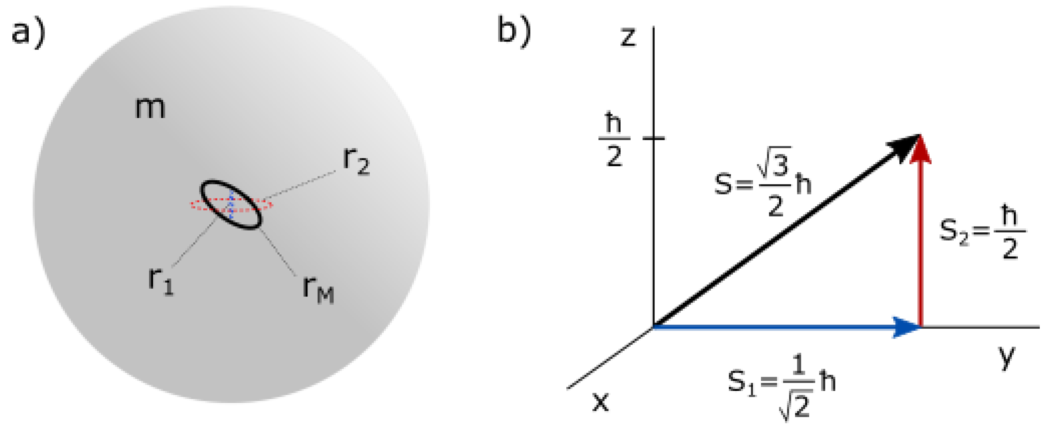
Consider a particle with 3 compositional charges. Suppose the spin momentum of each component of charge is equal to 1/2 ℏ in magnitude, and spins of two dominant charges are perpendicular to each other (having a [fixed] phase difference of /2 degrees). Two dominant charges now have a total spin momentum:
Total spin momentum of the particle includes the non-dominant charge (S2) as well, and is thus:
If the S2 charge momentum is perpendicular to S1, the value of total spin momentum is:
Due to fixed /2 phase and equal value, influence of components of S1 on the orientation [of the momentum projection] cancel (the two components may be interpreted as fermions in the same quantum orbital, so their projections cannot both be oriented in the same direction), and the orientation of the projection of the momentum S on the axis of quantization will depend solely on the orientation of momentum S2.
Note that, per the Pauli exclusion principle for fermions, S2 has to be on a different local orbital.
Note also that, in reality, there generally exists a difference between the spin momentum of mass and the spin momentum of charge (the source of magnetic moment). E.g., neutral mass and charge can be localized on different orbitals. This difference is reflected in the g-factor, the term used in calculation of the magnetic moment. Magnetic moment is proportional to the spin momentum but it has a different unit (involving other terms, apart from the dimensionless g-factor).
With the applied magnetic field, projection of the momentum on the magnetic axis (e.g., z) will thus be oriented either up or down:
This is a typical spin momentum of standard charges such as electrons and protons.
Figure 1a) shows charge in a localized state (as a particle) with acquired (coupled) real mass m, charge radii r1, r2 (corresponding to momenta S1 and S2, respectively) and radius of imaginary mass rM, here having a momentum aligned with S.
Figure 1.
Spin momentum.
The private space of such particle may be, depending on a reference frame, characterized either by properly scaled gradients or averages, of electric permittivity () and magnetic permeability () - or pressure and density.
With a decrease in environmental pressure (em/gravitational field interactions) a quantum may split into smaller quanta (which remain strongly entangled), spreading as far as possible (the range is finite and determined by the mass of smaller quanta - or environmental pressure on that scale), with a wave-like distribution of potential. Figure 2 illustrates the distribution of potential for such relatively free particle in a ground state. Total momentum is the sum of individual momenta. With delocalization, the quantum of energy will decouple from real mass m, but this may be synchronized with the dilution or explosion of mass m where individual quanta of m may be of appropriate scale and momenta to couple with individual quanta of img mass (this coupling is most likely to occur at the maxima of potential, which are also maxima in Figure 3).
Figure 3a) shows one interpretation of strength of forces of a wave with distance from centre (black = gravitational force, blue and red = electric force). Now each component (maximum) of a wave can be excited independently and may form moon charges, or may even merge with adjacent maxima under pressure. This allows the charge to interact (interfere) with itself in certain reference frames. Radial nodes (or, more appropriately, peaks) in Figure 3 can be interpreted as energy levels.
Figure 3b) shows how the private space of the same particle can be modified by interaction with another particle - essentially, the electric force has been exchanged for gravitational force. Such interaction may also collapse the wave into a particle with moon charges, where the number of moons depends on the equilibrium point of interaction (difference in energy of interacting particles).
Note that it is possible for the effect to be strongly localized - local space may be modified to attenuate one force and strengthen the other, while particles outside that space may not feel such [degree of] change.
Apart from the spin momentum, particles generally have an orbital angular momentum, and may be vertically and horizontally excited. Vertical excitation will be changing the nature of their dominant expression (e.g., from electro-magnetic to gravitational) and scale of energy (order of magnitude), while horizontal excitation will be evolving them through various similar forms (species) and energies.
On one vertical energy level their form may be dominantly wavelike, while on the other they may generally exhibit a corpuscular form. Energy levels are relatively discrete, and transition between them can be relatively instantaneous or continuous (interpretation depends on a reference frame), as required by CR. Both interpretations can, and generally do, exist relatively independently in reality. This is enabled through entanglement and coupling of energy between scales. Each form of energy thus has two components - real and imaginary (img) mass (charge). It can be stated that energy exists on various scales simultaneously, but interpretation is scale-dependent (generally, one form may be visible in dominantly electro-magnetic, other in gravitational spectra).
Quantization of properties, by the postulates of CR, must be relative. In reference frames where it exists, it may generally be correlated with the wavelike nature of energy at particular scale and described through [spherical] harmonics, as in quantum mechanics (QM). Localization (measurement) in some reference frames can be interpreted as transformation of a wavelike form of energy into a corpuscular form, however, this transformation is never absolute and better interpretation generally is wave confinement. Spin momentum generally has a non-zero mass/charge radius (it is thus an orbital momentum), although in some reference frames it may be approximated and treated as a point momentum.
5. Initial Structure Hypothesis
In planetary systems, outer planets (gas planets in case of the Solar System) are [groups of] electrons, while inner planets (terrestrial, in the Solar System) are [groups of] positrons whose gravitational maxima have been extracted from the system nucleus to balance the electrons.
Naturally, electrons and positrons here should be considered as relative electrons and positrons - not only has charge been exchanged for gravity, the associated gravitons may have settled in different mass eigenstates at the time of inflation, including tau and muon states. While certain properties should be conserved, the mechanism of charge-mass exchange also allows for fractional charge exchanges in transformational events (e.g., transformation of an electron into a down quark). In general, thus, outer planets may represent vertically excited negative charges, while inner planets represent vertically excited positive charges - or vice versa (in case of anti-matter counterparts). Relativity in positrons here may even be generally greater - they may typically represent quarks (but may also represent a physical interpretation of electron holes, which are usually considered as quasiparticles). It should also be possible for any of these to be paired with neutral fermions (e.g., neutrinos). All these possibilities will be explored later.
A planet can be in a 1e or 2e configuration (state), while the star is a relative superposition of nuclear partons (e.g., quarks). Inner and outer primary dwarf planets in a planetary system are considered to be bound and localized anti-neutrinos and neutrinos, respectively.
Here, 1e or 2e should not be interpreted as states holding 1×e or 2×e charges, respectively (where e is equal to the amount of charge of an electron) - the states may hold particles with fractional charges (e.g., quarks).
When it comes to regions (orbitals) dominated by charged particles (positrons/electrons), the configuration 1e should be interpreted as a state holding 1 charged particle (whatever its charge), while 2e should be interpreted as a state holding a pair of charged particles (whatever their charges are). However, charged particles can also be paired with neutral particles (e.g., neutrinos) - at least occasionally, if not regularly. If neutral particles are localized, they may fill local energy levels (associated with the orbiting particle, not the nucleus).
In case of regions dominated by neutral particles (neutrinos/anti-neutrinos), the configuration 1e should be interpreted as a state holding 1 neutral particle, while 2e should be interpreted as a state holding 2 neutral particles.
Primary components of the Solar System are shown in Figure 4.
In case of the Solar System, inner dwarfs (anti-neutrinos) or their remnants here are: Vesta, Ceres, Pallas, Hygiea (assumed to correspond to the number of neutrons in 10C). Possible primary neutrinos (outer dwarfs) are: Orcus, Pluto, Salacia, Haumea, Quaoar, Makemake (corresponding to the number of protons in 10C). Note that, in equilibrium, there should be 6 primary neutrinos present, however, some could be grouped together in 2e states, just like in case of planets (6 dwarf planets in the Kuiper belt may not all be primary neutrinos then, and some could be dead remnants - representing possible neutrino energy levels).
Note that, if positive charges are interpreted as electron holes, [anti-]neutrinos in between positive and negative charges could be interpreted as insulating barrier layers commonly present in Bose-Einstein Condensates (BECs) of excitons[5] (electron-hole pairs). In that case, for each pair, a distinct neutrino (barrier) should exist. This is indeed the case in the Solar System - in between 4 inner planets and 4 outer planets, there are 4 dwarf planets (or remnants). Now, the Solar System may represent a large scale Bose-Einstein condensate or its relative equivalent, but that does not imply that this condensate has been created by some large scale intelligence (it cannot be ruled out though). Such electron-hole combinations with barriers (relative event horizons) are probably common in atoms, note just in ultra-cooled atoms. Note that the high alignment (two-dimensionality) of orbitals also goes in favour of a BEC of excitons.
The current Solar System seems to have 10 nucleons, it may be the equivalent of a 10C atom, 10Be atom or a 10B atom, but the most likely may be a superposition (relative transition between two of these configurations), this will be explored in the following chapters.
Figure 5 a) shows the configuration of a 12C atom, on the left is the configuration of positrons (or holes), on the right is the configuration of electrons.
In this interpretation, energy levels are mirrored between positive and negative charges, relative to the [relative] event horizon(s) in between. This implies that the greatest energy concentration is at the event horizon (representing a nuclear radius), which has probably also been the initial state in the Solar System. However, the nucleus was localized and the horizon receded to the radius of the current Sun. The current barrier may then be also interpreted as a fossilized original barrier.
Figure 5 b) shows a possible configuration of a 10C atom at time of inflation (configuration unstable on standard scale, relatively stable on U1 scale - after nuclear localization).
Figure 5.
a) stable 12C energy levels b) possible Solar System (U1.10C) energy levels.
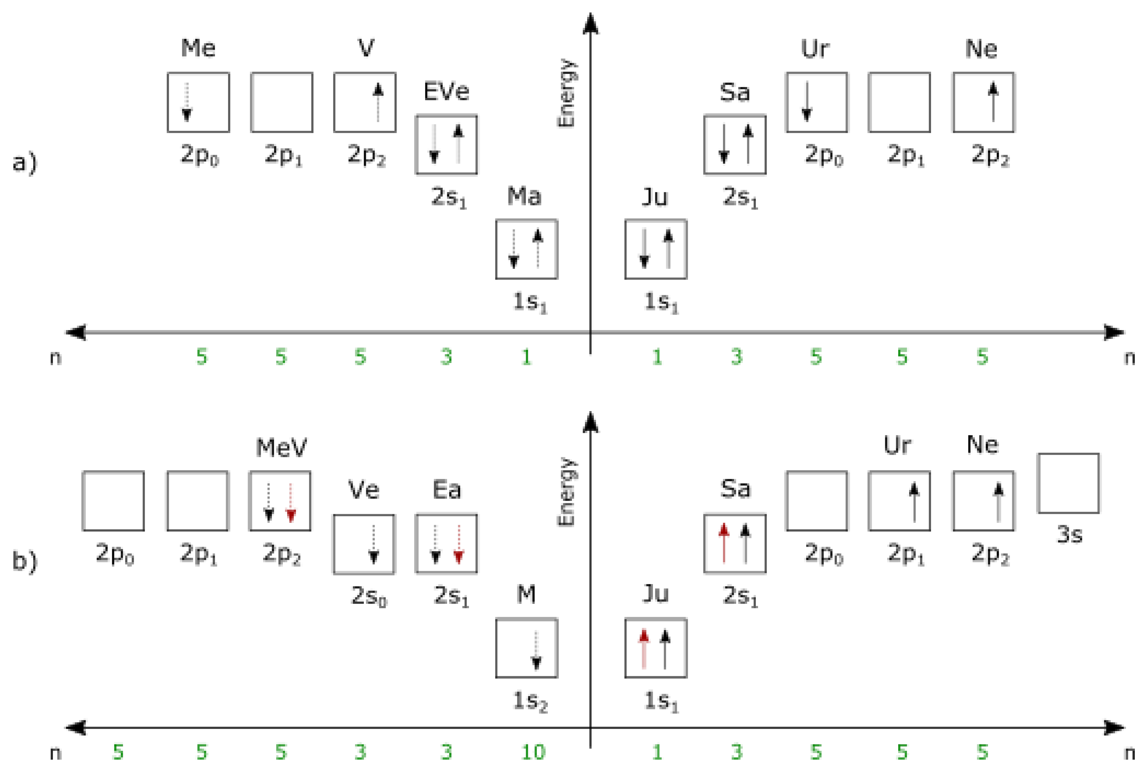
Note the splitting of s levels on the left side. This is illustrated as a possibility, but might not be the case in reality.
Due to multiple possible interpretations, principal quantum numbers here are shown with an excited value (n) and ground value (N) which here includes values 1 and 2. For the standard carbon atom in ground state the maximal principal quantum number is 2, equal to maximal N here (which means that electrons occupy states 1s, 2s and 2p, as shown in the figure). However, is it reasonable to expect for a system that has been vertically excited from the standard atom scale to the scale of planets to fossilize the ground state? The particles may have been in excited states prior to inflation. The values shown here are not random, they represent values derived later in the paper in some interpretations. Note that n on both sides seems to be inversely proportional to planet’s mass. Saturn is roughly 3 times smaller than Jupiter, while Uranus and Neptune are roughly 5 times smaller than Saturn. Mars is roughly 10 times smaller than Earth, however, either Mars’ or Mercury’s mass/location (or both) is apparently anomalous in this regard. This may be a consequence of mass oscillation. Note, however, that Mercury and Mars coupled together would be almost exactly 5 times smaller than Venus, so the anomaly may be the result of perturbation. In any case, should such anomalies be surprising, especially if the fossilized system is an unstable one, e.g., 10C isotope? Probably not.
Note also that 2 particles are allowed per sub-shell and there is no reason for a lone electron not to pair up with a bound neutrino, possibly forming a boson (e.g., W), although such pairing may be extremely unstable at room temperature/density, oscillating in existence (on U1 scale though, this state can be relatively stable).
In the Solar System, bound particles have been localized (forming planets and dwarf planets, with coupled real mass) and this affects the interpretation. However, localization does not imply loss of energy levels, they are simply localized as well, and some can be within the planet. Singlet, doublet and triplet states (involving neutrinos), all may be possible in localized energy levels. Generally, however, different particles occupy different energy levels.
Electric charge here is subdued (gravity dominates) and magnetic fields can be induced fields rather than associated with intrinsic magnetic moment (this is the case with Venus, for example, however, induced fields may exist within the planet as well). Also, time is slower on this scale (from our perspective) and real mass coupled to gravitons transitions continuously between energy levels. Planets then can appear to be in transition between states (which is unobservable in standard scale atoms). Some initial states may have been unstable at time of inflation (10C is unstable on standard scale) and this may appear fossilized due to slow evolution (continuous transition) of real mass (Venus and Uranus may be candidates for such states). Nevertheless, initial symmetry/inversion between inner and outer particles should be relatively conserved. In fact, the analysis here shows that many properties are conserved. The phenomena of horizontal energy levels and oscillation of gravitons are probably not limited to particles of standard scale (U0). If large scale gravitons exist, large scale quantization exists, regardless of the different nature of the dominant force. The Solar System may then be a proper large scale quantum system, rather than an inflated fossil of a quantum system. And this is unlikely to be limited to the Solar System.
5.1. General Deduction of Quantum Structure, and Possibly Stability
Here is an example how the element and exact isotope species can be determined from the number and types of planets.
The observed (star, planets) and hypothesized (dwarf planets) components of TOI-178 system are shown in Figure 6.
With the assumption of maximum 2 electrons (positrons) per planet, the TOI-178 system has these restrictions on the number of particles:
- 2 inner planets limit the number of positrons to 2 - 4,
- 4 outer planets limit the number of electrons to 4 - 8.
Since the intersection of the two groups contains only one solution (4), the TOI-178 system must be a Beryllium atom.
Note that this is valid for neutral atoms. In case of strongly ionized atoms, the determination of species must also take the mass of the star into account.
If the number of inner planets corresponds to number of neutrons, this must be a 6Be isotope.
This can be confirmed by comparing the mass of the TOI-178 system [star] with the mass of the Sun. Assuming that the Solar System is 10C (or 10Be), the determined mass of TOI-178 ( M⊙[6]) agrees well with the hypothesis.
However, the measured mass is still somewhat larger than expected - this will be resolved later.
Note that it may be possible for the number of inner planets to actually reduce with increasing number of neutrons due to increased gravitational potential provided by neutrons, but this also requires either low [properly scaled] temperatures/densities for condensation of charges beyond the 2e configuration (which is possible if not all particles are of the same species) or excessive number of neutrons compared to protons.
Thus, in heavy elements, due to condensation of mass and with no significant change in atomic radii, it may be possible for all planets of a system to be gaseous giants, where the number of charges cannot then be precisely determined from the number of planets. This may be unlikely though (condensation of mass/charge beyond 2e may be confined to the star radius). However, masses can be inflated due to mass oscillation. E.g., assuming U1 electron neutrino mass is on the order of the mass of Ceres, the mass of U1 tau electron neutrino would be on the order of 1024 kg. Mass oscillation should exist in all particles, leptons and quarks included. Thus, even inner planets in 1e or 2e configuration may become gas giants. However, symmetry/inversion should exist between inner and outer planets and it should be possible to make a distinction between inner, outer charges and neutrinos in between.
The number of bound [primary] anti-neutrinos should also correspond to the number of neutrons, while the number of bound [primary] neutrinos should correspond to the number of protons.
However, while bound anti-neutrinos/neutrinos should correspond to number of neutrons/protons, they may not be in the same configuration as positrons/electrons.
Thus, it is possible that TOI-178 has a single inner dwarf planet (holding 2 anti-neutrinos) instead of two dwarf planets, and two outer primary dwarf planets instead of four.
Interestingly, with the exception of the innermost planet, planets of the TOI-178 are in orbital resonance (18:9:6:4:3). The pattern does suggest one additional particle (or a binary) between the inner and outer planets, one that would complete 13 revolutions for every 18 revolutions of the second planet (pattern 18:13:9:6:4:3). Orbital resonances can be correlated with both stability and instability of orbits. In this case, resonances probably indicate stability. The lack of resonances with the innermost planet, and possible lack of the living dwarf (dwarf 13) in resonance, may be correlated with the instability of 6Be. In fact, the resonance may have been disturbed by the collision of the innermost planet with the dwarf 13, as the instability of isotopes, per the nuclear decay hypotheses in this paper, does involve interactions of inner particles (planets) with neutrinos (dwarfs).
Additional masses may also be bound to the system, however, orbitals of these should probably lie beyond the primary components, unless these are smaller homogeneous/undifferentiated masses not coupled to large scale gravitons (such as smaller asteroids and comets).
In case of the Solar System, there are no perfect mean motion resonances between inner and outer planets. However, apparent resonances do exist. These are considered coincidental as they change over time and could be lost relatively quickly. However, the presence of a near resonance may reflect that a perfect resonance existed in the past, or that the system is evolving towards one in the future, or both. In fact, oscillation of large scale gravitons can be correlated with the maintenance of the stability of the system - which can also include collisions of bodies of real mass as well, and may be further correlated with major extinctions of life on planets. Thus, the Solar System may be due for maintenance. Just like in case of TOI-178, the resonances associated with the innermost planet in the Solar System (Mercury) are the most unstable.
Obliquities (to orbit) of planets may also be correlated with system stability. Generally, a planet’s obliquity can be stabilized by the larger satellite (as is the case with Earth) or by differential motion of interior (as it should be the case with Mercury and Venus), but what is the source of obliquity? Conventionally, it is assumed to be a collision with another large body. Interestingly, in the Solar System, there are 4 planets (2 inner and 2 outer) with obliquities significantly deviating from 0, 90 and 180 degrees and 4 planets that are well aligned with these axes. This may then be correlated with the number of neutrons/anti-neutrinos in the system.
5.2. Singlet, Doublet and Triplet States in Planets
In QM, it is assumed that two particles in a singlet state share the orbital (at least with no energy level splitting involved). However, per CR, superposition (or entanglement) cannot be absolute and the two particles can have somewhat different orbital radii. On standard scale this difference may be unresolvable, but on large scale (U1) it can be. The difference may oscillate about relative 0, but interpretation involving fine energy level splitting may also be valid.
In any case, in 2e states there should be two major gravitons. In terrestrial planets one of these probably should be associated with the mantle, the other with the core. If these are in a singlet state, in equilibrium, there should be no differential motion between the core and the mantle. Again, however, per CR, the difference cannot be absolute 0, it must oscillate about the 0. The Earth seems to be in such configuration (as expected for 10C). Indeed, the rotations of Earth’s core and mantle are synchronized but oscillation has been detected as well[7].
Note that the detected rotation may be the rotation of real mass, but this should be [relatively] synchronized with the rotation of neutral [components of] gravitons (charge, or charged mass, can rotate differently).
Two gravitons are likely necessary for core/mantle differentiation (at least on shorter timescales of formation, and in case of lower initial densities of available real mass for planetary formation - in which case, the planet may not even form without the presence of a large scale graviton and its associated dark matter), but this differentiation probably exists even in 1e states due to [occasional, periodic?] coupling with neutrinos. If such coupling is temporary, differential motion between the core and the mantle should be higher after decoupling (as decoupling involves spin change) and the difference should be proportional to graviton mass (img mass), inversely proportional to real mass. If friction between mantle and core is low, the differential motion may be effectively fossilized at the time of decoupling. Indeed, pronounced differential motion in Mercury and Venus explains their [unexpected] low obliquity to orbit (differential motion has a stabilizing effect). Note that both, Mercury and Venus, should be, according to hypothesis (10C/10Be), in 1e states. This suggests they are, or were at some point, coupled with neutrinos.
Doublet and triplet states may be possible as well. Particularly interesting is the doublet state. Differentiated core may indicate a doublet state where inner and outer core have anti-aligned spins and no differential motion in equilibrium, but then there should exist a large difference between mantle and core rotation.
However, there are other, probably more likely, interpretations. One of them is splitting of energy levels, the other is oscillation between local energy levels.
Differentiation of the mantle into layers, for example, would then be relatively synchronized with the oscillation of a graviton between local energy levels (which themselves may be the result of splitting of the primary mantle level). And the causality here is relative, in some cases the cause for differentiation or creation of discontinuities (two adjacent layers don’t have to be of different chemical composition) may be the graviton, in others real mass. What drives energy level changes depends primarily on mass difference between img (graviton) mass and real mass. Dominant force may vary with time, in the early days of formation, the graviton is probably the dominant driver. In any case, most appropriate term here is synchronization, rather than causality. One is simply transitioning continuously, the other in discrete jumps. Note that this mechanism of evolution allows for higher plasticity in planetary characteristics, e.g., core differentiation and solidification in a planet may be a transient and periodic phenomenon, allowing for periodic re-establishment of a magnetic field. In equilibrium however, disturbance by external force (e.g., asteroid impacts) is likely required for energy level changes.
5.2.1. Correlation with Planetary Atmospheres
Assuming large scale gravitons of terrestrial planets like Earth have mass on the order of 1019 kg (as established in later chapters), equal scaling gives mass of localized large scale anti-neutrino/neutrino gravitons on the order of 1015 kg - 1016 kg. These gravitons are generally coupling to bodies of real mass on the order of 1019 - 1020 kg (inner dwarf planets). Interestingly, this is on the order of mass of Venusian atmosphere. If Venus is coupled to a neutrino than this graviton could act as an gravitational attractor in Venusian atmosphere (assuming the graviton radius is on that level).
What is the shape of this graviton? This should be correlated with the shape of the atmosphere. In this case the graviton should be spherical, or torus-like.
This could then help sustain life in Venusian atmosphere and may have a role in the long-term stability of its extreme super-rotation.
Note that the graviton doesn’t have to be present all the time - it could be periodically inflated (delocalized) to this radius (assuming the neutrino is coupled to the planet, otherwise, the process should include both inflation and deflation - assuming neutrino is initially coupled to an inner dwarf planet in the asteroid belt). The presence of atmosphere in a planet then may generally indicate a [periodic] presence of neutrino gravitons. Another interesting case is the thin atmosphere of Mars, its mass is on the order of 1016 kg - hypothesized mass of a naked neutrino graviton (thus, depending on interpretation, half of the mass could be in the coupled graviton). Mercury has no significant atmosphere (its mass is less than 104 kg). All this suggests that Venus, Earth and Mars are all [periodically?] coupled to neutrinos (which may imply triplet states in case of Earth and Mars), while Mercury is not. With 3 neutrinos coupled to planets, and assuming a 6p4n state of the Solar System, only 1 neutrino should be coupled to inner dwarfs. And that’s probably the active one - Ceres. The mass of Earth’s atmosphere is on the order of 1018 kg and the Earth is probably transitioning from one extreme to the other (e.g., Mars -> Venus). Interestingly, the mass of Earth’s atmosphere varies annually on the order of 1015 kg (mass of a naked neutrino graviton). Could this variation indicate the presence of coupling? And do states on Venus and Mars represent fossilized end-states or are these two at the end/beginning of a cycle? If that is the case, and all these cycles are relatively synchronized, the Earth should be at the end of an atmospheric cycle as well, which would suggest relatively imminent rapid changes in Earth’s atmosphere.
5.3. General Stability of Gravitons
Stability of isotopes of standard atoms depends on the proton/neutron ratio and the number of bound neutrinos and anti-neutrinos, which is correlated with that ratio. Periodic coupling of particles with neutrinos could ensure spin (obliquity) and orbital stability (e.g., by resetting eccentricity/resonance).
According to the presented hypothesis on decay, the isotope is destabilized if a certain particle localizes at the point where it can overcome the barrier correlated with the strong force. If the particle occupying the barrier has an eccentric orbit, the probability of destabilization (decay) is proportional to that eccentricity (as the strength of force falls of sharply with distance, localization of the interacting particle at apoapsis increases the probability that the force will be overcome). During localization/delocalization cycling, particles probably periodically couple with neutrinos. The cyclicity is not perfect and the period can deviate from the average. The higher the period is the lower the resonance becomes (which, in this interpretation, implies higher eccentricity) so the probability for decay increases.
According to the previous chapter, Mercury is not coupled to a neutrino and its high orbital eccentricity goes in favour of instability in this interpretation. Indeed, even in conventional models, Mercury’s orbit is relatively unstable[8]. Per the decay hypothesis, as the decay occurs, a wave is emitted carrying information about the collapse (probably some species of a graviton neutrino) and this wave is absorbed by the atom of the same element (species) as the atom that decayed. Absorption of this energy resets the ageing of the atom, by increasing resonance (stability of cycling).
This process in some form (evolved) probably exists in any entangled community or organization of the same or sufficiently similar species. Consider a human family, for example. If humans, like atoms, have souls (even if relatively more complex), death of a human probably involves emission of particles (waves) on some scale and these are then probably absorbed by another human [soul], affecting its physiology (epigenetics), which may even be, at least in some cases, correlated with temporary ageing reversal or acceleration. This is, what I believe, I have experienced about the age of 36. But I believe I have seen this change in others as well. The probability for absorption should be directly or indirectly proportional to the entanglement between individuals, which is also proportional to the genetic match between the deceased and the absorber. This implies that DNA is correlated with the properties of this kind of souls. I have explored soul-body couplings in more detail and correlated them with consciousness in other papers.
6. Quantum Nature
Even though the dominant force on this scale is gravity, being formed through the inflation/deflation of gravitons (conserving many small-scale characteristics), the Solar System can be modelled as an atom with 10 nucleons. Here I assume this is a large scale 10-Carbon isotope equivalent. Due to specific conditions some of its components are at the lowest energy level - multiple nucleons are condensed into a single nucleus, orbitals are two dimensional (collapsed from spherical cloud structure), highly aligned (same plane), and momentum carriers are [scaled] point-like structures - they are strongly localized.
Relative scale invariance of physical laws (as postulated in CR) requires that non-dimensional ratios - those of radii, masses and velocities (energies in general) in two systems of the same species (carbon in this case) in the same state but of different scale (vertical energy level) are equal.
Scale invariance in CR is relative scale invariance. Non-dimensional ratios are preserved between different vertical energy levels but the constants have different values (unless the metric is scaled as well).
Radius of the outermost electron in a standard 10C atom can then be obtained from Neptune spin and orbital radius:
This gives [localized] electron radius = 3.834298096 × 10⁻¹⁶ m. Note that radii of particles inside the atom can be different than outside of the atom (radii depend on localization energy).
Note that, in this paper, results of calculations may commonly include many decimals - suggesting high precision, however, in a lot of cases this interpretation is wrong as variables in the equations commonly have varying precision and uncertainty. Since the paper is constantly updated and high precision is usually irrelevant for the aim of this paper (only the most significant digits are usually relevant, less significant digits usually should not be taken seriously), in a lot of cases I did not bother rounding the values. However, in the final version of the paper, the values should be properly rounded, with stated uncertainties.
Sun core radius from 10C nucleus radius and outermost electron radius:
The above gives Sun core radius of 173894.6069 km, or 1/4 of the apparent Sun radius, in agreement with experimentally obtained values of Sun core size. More precisely, this is the Sun’s outer core [discontinuity] radius and also [approximately] U1 classical electron radius.
The values of constants used here are values listed in chapter 3. Constants.
Proton radius approximation:
The factor P/N = 6/4 = 3/2 is the ratio of protons to neutrons in Carbon-10 (10C) atom, factor 10 is the number of nucleons (P+N).
The above gives 0.722296 × 10⁻¹⁵ m = 0.722296 fm for the proton radius, close to the experimentally obtained value of 0.8414(19) fm (2018 CODATA[9]).
The same result can be obtained using spin radii:
A precise value can be obtained by taking into account the influence of quarks instead of P/N (this will be elaborated later):
which gives 0.8426785306 fm, a value in agreement with the CODATA value.
Note that the value used for the 10C charge radius in equations above is the covalent radius. Using covalent radius produces much better results than using van der Waals radius, suggesting that the Solar System was inflated as a binary system. This should not be surprising, considering that 85% of stars exist in binary systems or systems with three or more stars[10], and about half of all Sun-like stars are binaries[11]. Evidence suggests that all stars form initially as binaries[12], and evidence exists suggesting that the Sun indeed likely had a binary companion at the time of formation[13]. However, covalent radius is also more likely to represent a proper atomic radius of non-bonded atoms and can be equal to the outermost electron orbit of a non-bonded atom. Van der Waals radius is more likely to include the outer neutrinos and could be equal to the outermost neutrino orbit.
Radius of the proton cannot be absolutely constant, due to hypothesized entanglement between vertical scales, apart from required oscillation, it should probably be shrinking as the universe expands.
Comparing masses:
This gives:
The above shows mass ratios agree not only to the order of magnitude but are actually very close in value. The excess energy is:
and it must be the accumulated relativistic energy of the Solar System (discrepancy arises due to different reference frames in the mass measurement - the mass of the standard 10C atom is measured from an external frame, while the mass of the Solar System is derived from within the system and improperly treated as rest mass).
Although the Solar System is at rest relative to us, relativistic energy (deviation from rest velocity) of the system relative to underlying space is always locally real and must be stored somewhere within the system. The likely capacitor is local space of the system and the energy is stored in the form of gravitational potential.
If the energy is stored mostly in the Sun, this would imply non-homogeneous storage of kinetic energy as gravitational potential - likely proportional to the scale of the large scale gravitons.
However, it is also possible that energy was accumulated before the birth of planets. Most likely, this energy was accumulated with nucleus inflation during the conversion of electro-magnetic potential to gravitational.
Of course, the Sun loses energy over time but lost mass is on the order of 1027 kg, significantly lower than hypothesized relativistic energy.
There are other possibilities for excess mass acquisition, however, acquisition of mass on the order of 1029 kg is, after inflation, probably unlikely, especially considering distances and motion of bodies in the galaxy.
From this one can calculate the scaled limiting speed of light (information) for the U1 scale (c1):
If v is interpreted as the cumulative velocity against the CMB (Constant Microwave Background) radiation, a sum of secondary velocity vs (velocity of the Solar System against CMB) and primary velocity vp (equal to velocity of the local galactic group against CMB), for vs = 368 km/s and vp = 628 km/s, one obtains:
Obtained c1 is equal to one of the possible values calculated in CR[14], but will also be confirmed here later in a different calculation.
At first, it might seem that this calculation cannot be valid since both velocities are relative to CMB and vp should not be included in calculation. However, the obtained c1 is confirmed later. This puts certain constraints on the Sun’s evolution, suggesting that the Sun’s graviton (or, superposition of large scale gravitons) was, with initial inflation, accelerated to 628+368 km/s (996 km/s) in the same direction as the local galactic group (possibly the velocity of the Milky Way was equal to the velocity of the local galactic group at the time), then decelerated to 368 km/s, however, not losing the acquired energy (it is yet to lose it on U1 scale).
This energy conservation becomes plausible with hypothesized duality of energy transition taken into account - on one scale transition is quantized, on the other continuous. Here the energy of the graviton is quantized and requires certain time to collapse to lower energy level. Indeed, the Sun is continuously losing energy in the form of electro-magnetic radiation, but the spent fusion fuel remains inside and may be expelled all at once in a bigger amount (this quantization of [the loss of] kinetic energy is confirmed later, where it is shown that the calculated kinetic energy is exactly equal to the energy of a single excited large scale neutron). Note that the spent fusion fuel so far is on the order of the acquired kinetic energy (this is calculated in the chapter 19.3. Energy replenishment, burning cycles). Associating this fusion fuel with the acquired energy and the Sun’s large scale graviton, it would be reasonable to assume that its collapse [to a lower level] would occur once fuel spent in fusion becomes equal to the acquired relativistic mass (ΔM) - when all of this mass will be expelled. This may be further correlated with the hypothesized cycling of the Solar System (chapter 9. The cycles).
However, alternatives exist for the proposed kinetic mechanism. Another possibility is that the accumulated energy corresponds to the current speed (368 km/s), but the mass of Neptune has been decreased instead, from 1.08 × 1026 kg to 1.02 × 1026 kg (current mass). The actual solution may be a superposition of the two. Assuming that the initial Neptune mass was 1.05 × 1026 kg (not a randomly chosen value, it is the average of the two but also, as shown later, the rest mass the Neptune should have had assuming it is a muon electron equivalent), the acquired kinetic energy becomes 7.124 × 1028 kg. To obtain the same c1, a velocity v of 777.250 km/s is needed. Interestingly, assuming part of this velocity is equal to the current Milky Way’s velocity relative to the CMB (552.2±5.5 km/s[15]) or to the escape velocity at Sun’s position ( km/s[16]), the other part becomes equal to 225.1±5.5 or km/s, respectively, suggesting it is equal to the Sun’s average orbital velocity (230±3 km/s adopted, 228±2 km/s mean weighted[17]) in Milky Way. In this case then, the accumulated energy may not be the energy relative to the CMB (or at least not completely), rather energy acquired from local space (associated with Sagittarius A*). The most plausible scenario probably involves the Sun’s graviton inflating from a region closer to the galaxy centre, reaching maximum velocity of 777.250 km/s (or 996 km/s, depending on interpretation), slowing down due to attractive central force and converting the momentum to the angular orbital momentum in the process.
Comparing masses of systems of different scales requires proper relativistic treatment. Apart from the speed of light being different between the scales, a proper reference frame must be chosen. In case of comparison of U1 scale system (such as the Solar System) with an U0 system (such as a 10C atom) a proper reference frame is probably the CMB (Constant Microwave Background) radiation rest frame.
Proper equation is thus (for v1 = v0 = v):
v = v⊙ = cumulative speed relative to CMB = 996 km/s
c1 = speed of light on U1 scale = 2.93 × 10⁶ m/s
c0 = c = speed of light on U0 scale = 2.99792458 × 10⁸ m/s
Note that CMB radiation is of U−1 scale (the hypothesized scale of space forming particles of U1 systems).
Note also that the maximum speed (cn) depends on pressure and density of space and it is generally not equal to the standard speed of light. Here thus, even though the term speed of light may be used, c1 should be understood as maximum speed of U1 scale information, and also particles (stars) in local space.
Within the galaxy, speed limit for orbiting bodies is generally defined by the gravitational maximum (event horizon) of the well - stars orbiting galactic centres with semi-major Keplerian velocities larger than c1 could exist in other galaxies.
One can now attempt to resolve the excess mass of the TOI-178 (6Be) system. Assuming its velocity [relative to CMB] is 77.22 km/s larger than Sun’s velocity, its mass should be:
= rest mass of a 6Be atom = 6.0197 u
= rest mass of a 10C atom = 10.016853 u
M = rest mass of the Sun (relative to CMB) = 1.870062271 × 1030 kg
v = cumulative speed of TOI-178 relative to CMB = 1073.22 km/s
However, mass of TOI-178 obtained from measurements is 0. M⊙[6].
Apparently, measured mass is bigger by the relativistic [omega] factor:
The cause of discrepancy is, again, in the reference frame - calculation is done relative to CMB, while measurements were done from the Solar System (Earth) reference frame.
From such reference frame Sun is at rest and its rest mass is equal to relativistic mass relative to CMB, M⊙ (1.988500 × 1030 kg).
However, one must take into account the radial velocity [relative to the Sun] of TOI-178. Relative to the Solar System, the mass of TOI-178 should thus be:
= radial velocity of TOI-178 = 57.4±0.5 km/s
This gives 0.650 M⊙ for the mass of TOI-178, in agreement with measurements.
Note that relativistic effects are always physical, but not always on the same scale and not always in the same space - e.g., some may be physical in the space of the observer (in which case the effect on the observable is illusionary), some in the space of the observable, or in both to certain degree[18].
Solar System is thus a [negatively] polarized reference frame relative to TOI-178 and to convert the measurement to a proper [neutral] reference frame, one must multiply the measured value with a positively polarized omega factor:
Note also that TOI-178 is the only system I have analysed beyond the Solar System. The reason that an effectively randomly chosen system fits the hypothesis goes strongly in its favour. All planetary systems close to the Solar System, and probably all systems in the Milky Way, should conform to the same speed limit. However, I find that analysing all these is beyond the scope of this paper. Hopefully, other researchers will do these analyses eventually.
6.1. Validating Rest Mass and 10C/10Be Configuration
If the Sun is a large scale equivalent of an atom nucleus containing 10 nucleons, one can calculate the mass of a proton (hydrogen) equivalent on large (U1) scale:
Mp = standard proton mass = 1.67262192 × kg
= standard 10C nucleus mass = 1.663337576 × kg
M = previously calculated Sun rest mass = 1.870062271 × kg
And this is on the order of red dwarfs - smallest known stars, in agreement with the result.
One can then assume that no star in the observable universe should have a mass smaller than this at times of creation (after inflation).
Observations seem to be in good agreement with this. Until recently, the star with lowest known mass was considered to be the AB Doradus C, with a mass of 0.090±0.005 M⊙[19] or 94.3±4.7 MJ (Jupiter masses) - in complete agreement with the above. However, more recent evidence indicates that this might not be a star, rather a binary of two brown dwarfs[20]. The current record holder is considered to be EBLM J0555-57Ab, with a mass of 85±4 MJ (0.081±0.004 M⊙)[21].
Of course, stars are losing mass over time. Assuming maximum age of universe of 13.8 × years and knowing the rate of ageing (mass loss) of red dwarfs, one can calculate what mass would a red dwarf with initial mass of 0.095 M⊙ (99 MJ) have at this point. All of these stars should still be alive and on the main sequence (it is expected for stars of this mass to remain on main sequence for over 6 trillion years, with total burning lifetime of about 10 trillion years).
Assuming average luminosity of 3.29 × L⊙ for a typical 0.095 M⊙ red dwarf (luminosity based on 0.095 M⊙ Scholz’s WISE J0720-0846A[22]), mass at this point would be:
t = age of the universe = 4.3549488 × s
mp = standard proton mass = 1.67265 × kg
Er = energy per reaction = 4.32 × J
P = power output = 3.29 × × 3.8 × J/s
N = fraction of mass used in fusion = 2/3
Mass loss through radiation is thus almost negligible, but one must also account for the loss of mass due to solar wind. Mass loss through solar wind for cooler stars is estimated to be higher than that of the Sun[23], assuming mass loss rate 10 times higher for 0.1 M⊙ dwarfs (which may be conservative), mass at this point should be:
Mr = Sun mass loss rate = 2.5 × M⊙/yr[24] = 7.922022 × M⊙/s
Considering that red dwarfs with lower mass have been observed (assuming they are indeed red dwarfs), the result suggests that either the assumed mass loss rate is indeed conservative (but not much) or the universe may be a bit older. However, the excellent agreement of the result with AB Doradus C suggests otherwise - perhaps AB Doradus C is not a binary after all rather a proper red dwarf, while smaller ones - like EBLM J0555-57Ab, may be binaries, or should be classified as brown dwarfs?
6.1.1. Remnant Hypothesis
Brown dwarfs may be, dominantly, remnants of dead stars (instead of protostar material), just as asteroids and comets may dominantly be remnants of dead planets and moons. If stars generally have multiple gravitational maxima (as I do hypothesize), once the gravitons decouple from the body of matter (real mass), it should not be surprising if dead aggregates of matter are, due to significant angular momenta, kept separated - forming binary systems (in most cases). One of the binaries should represent the remnant of the star’s core while the other should be the remnant of outer layers. Distribution of mass between them should generally be asymmetric.
Moment of inertia puts constraints on density distribution inside bodies. Based on this, it is estimated that Sun’s core contains about half of the mass of the Sun. It is also considered that the Sun’s core radius is 0.2 - (Sun’s radius) but exact distribution of mass here is unknown. Based on the hypothesis of multiple gravitational maxima correlated with large scale gravitons, I argue that the Sun’s inner core is not bigger than and that most of the mass is in the region about . The inner core then has a significantly lower mass than assumed. In a later chapter, I have calculated that this mass is only several times Jupiter’s mass. At the end of its life, the Sun leftovers are probably going to form a binary system of a white dwarf (remnant of outer core mass) and a brown dwarf less than 10 times the mass of Jupiter (core remnant, which may still be alive and act like a gas planet, as decoupling of gravitons is relatively synchronized, not absolutely).
I assume that, with decreasing star mass, the outer mass is decreasing while core mass is increasing (due to detected generally smaller angular momentum of smaller stars) - they may be absorbing helium ash produced in outer regions at least to some degree (nuclear fusion does not occur in the inner core in this model). Remnants of red dwarfs should then be brown dwarfs, where one should be about 80-85 times Jupiter mass (0.075 - ) while the other (core remnant) would be on the order of 10 times Jupiter mass. Distance between these binaries and their masses would then be generally proportional to the original size of the star.
The study indicating AB Doradus C is a binary, does provide masses conforming to this ratio, 0.072± and 0.013±[20].
Is AB Doradus C an ageing red dwarf revealing presence of multiple gravitational maxima or indeed its remnant - which would imply its death was violent or that it represents a remnant from an older universe?
In any case, decoupling of gravitons from bodies of matter is generally a change of energy level (a vertical one, in this case) so it occurs with spin inversion, explaining lower rotation periods of dwarfs compared to bigger (original) bodies.
Decoupling/disentanglement is not absolutely instantaneous. Thus, during graviton spin change, real mass should experience some gravitational dragging - slowing its rotation.
If remnant core mass is increasing while outer mass is decreasing (with decreasing original star mass), remnant binaries with roughly equal mass should be possible. According to the above, their masses should be about 40 times Jupiter mass.
However, original system can also be a binary system with stars having similar masses. Therefore, equally massive binary remnants with masses smaller than (perhaps with a wider orbit as well) are also possible. With differently sized original companions, different remnant companions are possible.
This can then explain the recently discovered abundance of Jupiter-mass binary objects in the Trapezium cluster[25] - something highly unexpected with conventional theories on formation of planetary systems.
These objects were probably not planets ejected from original systems (as some suggest but struggle to explain), rather, they represent in situ remnants of stars. However, it should be clear that at least some of these could also have been created with the inflation of unbound (free) [pairs of] standard particles, like tau electrons.
6.1.2. Dark Shade of Glue
A body gravitationally coupled to a large scale (U1) graviton (gravitational maximum) is, more precisely, a body coupled to its space, which is usually in the form of spherical, torus-like, or ring-like haloes composed of gravitons of smaller scale ().
This is an example of vertical entanglement (entanglement between different scales of energy).
More complex formations of space are possible (e.g., in the form of tubes or filaments), however, these are commonly associated with specific horizontal entanglements between gravitons and may be considered as different dimensions of space, existing independently of the private graviton space. However, coupling of the space-forming gravitons to matter generally includes graviton transformation, which, with significant change in scale, can distort the local space and transform the vertical entanglement into a more horizontal entanglement.
Once an U1 graviton decouples from the body of matter this glue of scale holding matter together should lose stability and start to dissolve - flattening the space (dissolving the entanglement with the parent U1 graviton). The body of matter can still remain clumped (held together by electro-magnetic forces or by the gravity of still smaller scale) but will lose energy faster than the body coupled to a large scale graviton and will tend to spread out (unless recycled by new coupling) due to increased vulnerability to cosmic disturbances. The vulnerability is increased not only due to the weakening of the glue but also due to the loss of orbital stability (orbital stability of large scale gravitons is likely periodically maintained through the maintenance of orbital resonance).
Note, however that, due to the relativity of causality, sometimes the glue will start dissolving before the decoupling.
One must distinguish then a [still] living remnant from a dead remnant. In example, the outer part of the Sun may not collapse to form a conventional (long-lived) white dwarf, rather disintegrate and spread as a nebula. However, if the core remnant is still alive and massive enough, the material could form a shell about it (but will eventually sink to the centre as it should be composed of heavier elements than the core). Common white dwarfs could actually be such objects. In that case, a white dwarf with a carbon envelope should be relatively young (older ones should be surrounded by helium and hydrogen, with carbon in the core). Note that, in such scenario, the gravitational well of the [U1] core graviton becomes over-capacitated - decreasing its lifespan (increasing probability for premature death).
A good analogy to dark matter holding ordinary matter (real mass) together can be found in hyphae of living fungi holding soil together (preventing erosion). A good analogy to an over-capacitated core is an overweight person.
If asteroids are remnants of dead bodies, the particles they’re composed of should not be held together by large scale dark matter halo and filaments. If then a theory of gravity does not distinguish between different scales of gravity, or - in other words, does not distinguish between living (graviton entangled) and dead celestial bodies, applying its laws to one of these can result in anomalies in certain cases (due to misinterpretation of phenomena or understatement/overstatement of certain quantities - like mass/density and mass loss).
Young asteroids (or, generally, asteroids with non-dissolved gravitational glue associated with large scale coupling) are then less likely to disintegrate as they pass through an atmosphere.
However, any asteroid passing through atmosphere is disturbing bodies in that atmosphere and can couple to local gravitons if these are/become available - if the local well is undercapacitated there will be available gravitons for coupling, if not, death (decoupling) events are required to enable new couplings (however, violent interaction with the atmosphere can involve local decoupling events).
Celestial bodies not entangled with U1 gravitons (or, properly dead bodies) should represent clumps of matter loosely held together. Effectively, the gravitational constant between the components of these bodies is reduced (the effect of running gravitational coupling) and this should be verifiable experimentally (providing the quantity of mass can be precisely determined - without involving gravity). I assume that electro-magnetic coupling of elements is not noticeably affected so the effect should be most pronounced in non-polar intermolecular bonding, especially between less massive (less polarizable) molecules and higher intermolecular distances (e.g., at high temperatures) - as induced dipole attraction falls sharp with distance.
In, here assumed, interpretation of graviton-body (soul-body) coupling there is no mass shielding so the total mass of the system is the sum of ordinary and dark matter mass. Thus, the force one usually attributes to ordinary mass should generally be attributed to the sum of both masses. With that neglected, bodies lacking dark matter (such as certain asteroids) may be observed anomalously accelerating (as their coupling to gravity is limited).
Indeed, such anomalies associated with asteroids have been observed recently (e.g., ’Oumuamua, DART[26]).
Note that interstellar visitors are more likely to show anomalies as they are generally not entangled with local U1 gravitons and probably not entangled with any remote ones as well. The anomaly should, however, only be present if the local coupling/entanglement capacity is full.
An asteroid ejected from Mars millions of years ago, in example, can still be entangled with Mars’ U1 graviton and may not show any anomalies - especially if the graviton wasn’t changing energy levels in the meantime.
In another example, any kind of a satellite launched from Earth will carry coupled gravitons which will remain entangled with Earth’s U1 graviton - no matter the distance, until this entanglement is disturbed, either by Earth’s loss of consciousness (temporary or permanent U1 graviton decoupling) or satellite entanglement with another U1 graviton.
If the hypothesis is correct, with more visitors more anomalies should be observed. But more local surprises[27] cannot be excluded as well.
As weakening of intermolecular bonds (weakening of localized G) can precede U1 graviton collapse, such weakening detected on Earth could be interpreted as a precursor to large scale weakening - collapse (de-localization) of the Earth’s U1 graviton.
This weakening should cause Earth to expand a bit (first partially then globally). And this could (due to the proportionality of the effect to element mass) cause some degassing. Again, due to relativity in causality, degassing can start before the expansion - albeit involving a different reason/mechanism (e.g., current degassing is correlated with climate change). I believe all major extinctions and correlated climate changes are also correlated with temporary graviton collapses. Nature isn’t picky when it comes to causes and precursors for certain effect. Therefore, the effectively induced actions leading to certain effect can be, over time, diverse, even anthropogenic.
Increase in seismic activity (including volcanism) can also be correlated with the changes in inter-molecular bonding. Not only that, but precursors of collapse may have a wave-like distribution with increasing frequency over time. Allowing certain predictability of seismic activity[28].
6.1.3. Plastic Density
It was noted previously that applying conventional theories to asteroids can yield anomalies. Particularly interesting ones are anomalous masses or densities, like the one in 33 Polyhymnia and similar bodies. Polyhymnia is a spherical body in the main asteroid belt with a 54 km diameter and estimated density of 75.28±[29]. This extreme density cannot be explained by known elements so it is considered unphysical and most likely a result of measurement errors (which is certainly possible as determination of mass of bodies like Polyhymnia is extremely hard). However, Polyhymnia is not the only asteroid with anomalous density and I believe these cases deserve further investigation. Assuming these are not highly compressed remnants (of cores of giant planets), these could represent [almost naked] large scale gravitons. The shape here is important. Polyhymnia is a very good candidate due to its spherical form (a form of a graviton in ground state) which would be, otherwise, unexpected for such small body.
Interestingly, the study of Carry on density of asteroids[29] suggests clumping of bodies of very variable densities on the same order of mass, 1018 - 1019 kg (including Polyhymnia), while, as it will be shown in later chapters, I have determined that Earth’s [large scale] graviton mass is on the order of 1019 kg.
Since gravitons aren’t supposed to have highly variable masses (their masses should be relatively quantized, coupled real mass should be more variable, as well as their size), one explanation for the clumping could be that most of these bodies are coupled to a graviton of the same species (e.g., 1018 kg or 1019 kg). These bodies thus, apart from the dark matter associated with the graviton, are not composed out of heavy exotic elements (which would require existence of islands of stability in the periodic table of elements) - rather, the img component of total mass dominates, while their real mass (standard matter) could be much lower and much less dense. Most of these bodies could simply be dusty or icy gravitons (low mass/density of standard matter, high gravitational mass) and I would like to see at least one of these bodies further investigated, especially Polyhymnia.
Alternatively, some of these bodies may be remnants of giant planets. This is also unexpected by conventional theories, however, I have predicted [re]cycling of planetary systems (explored in later chapters). Therefore, Polyhymnia could be a remnant of the core of a Jupiter-like planet as well. In that case, it should be older than the current Solar System. Its aphelion may then be a relative fossil of a semi-major axis of a Jupiter-like planet in the previous cycle. On the other hand, if it is a relatively naked graviton, it could represent a placeholder for a Jupiter-like planet’s core in the next cycle (I assume Jupiter-like bodies contain multiple gravitational maxima - at least two, core graviton is only one of them).
6.1.4. Distinguishing Living from Dead Bodies
Living bodies are active bodies and require energy to sustain that activity and prevent decay. Components of a living body are mutually entangled, exchange energy/information and are themselves habitable for life of smaller scale. In case of planetary systems, a habitable planet is usually a living planet itself, however, a planet may remain habitable for considerable time even after death. Celestial bodies can give and receive energy through standard radiation (electro-magnetic, gravitational, particle emission), tidal interactions, accretion/collisions, and large scale gravitational waves. This energy can be conserved for longer intervals in the form of residual heat and radioactivity. One can assume then that living bodies which are most of the time far away from sources of energy prioritize energy accumulation over radiation. Living bodies farther away from sources of radiation will prioritize tidal interactions and other energy sources. Most likely candidates for living bodies are thus energetic bodies (but possibly not in the extreme, although extremophiles likely exist on any scale and planetary extremophiles could even contain relatively isolated more habitable areas) entangled with other living bodies.
In case of warm-blooded bodies (lifeforms that normally emit more radiation than they absorb), such as stars, gas giants and probably ice giants as well, it should not be so hard to distinguish living from dead bodies. In the Solar System, Jupiter, Saturn and Neptune are all emitting significantly more radiation than they absorb. Uranus, however, appears to be in thermal equilibrium[30], suggesting that it may be dead. In terrestrial planets, however, thermal equilibrium is not an unambiguous signal in this context. One indicator of death that may be applicable to all planets, is a significantly lower mass and a change in radius of the body compared to the established rest mass/radius for the species. Here again, Uranus has a much lower mass than Neptune and a bigger radius, although the two belong to the same species (Neptune mass is very close to the rest mass average here - as it will be shown later, both Uranus and Neptune probably represent large scale muons).
Note that the amount of radius change will depend on temperature and the state of mass, but also on the mass and mass radii of previously coupled gravitons. In gaseous planets radius is most likely to be inflated. For terrestrial planets, some shrinking of radius is probably more likely with graviton decoupling (which should, however, be preceded by small temporary expansion). Even though the gravitational mass is decreased here as well, this decrease should be much lower (at least in case of non-violent death). The decoupling will, however, affect the stability and angular momenta of layers. It is the collapse of solid outer layers, coupled with the expulsion and loss of volatiles, that should cause overall contraction.
High obliquity to orbit, unexpected lack of rotation and the absence of hydrostatic equilibrium are other potential indicators of death.
Decoupling of gravitons from bodies is not absolutely instantaneous and will, due to spin momentum inversion, certainly affect rotation of the remaining body. The magnitude of the effect, however, depends on the ratio between img (graviton) mass and real (body) mass.
The intensity of tidal heating is proportional to the square of the orbital eccentricity[31] - being zero in a circular orbit and reaching a maximum in a parabolic orbit, and inversely proportional to the size of the orbit. One might consider a simple case of tidal heating between two bodies, but this is generally an n-body problem and may include many entangled bodies.
In case of celestial bodies, gravitational entanglement is a primary entanglement, in terms of energy exchange, with orbital resonance being the secondary component.
In an example, one might consider large bodies of the main asteroid belt - Vesta, Pallas, Ceres and Hygiea. Of these, Ceres is a dwarf planet, others are probably remnants of dwarf planets.
Entanglements can be positive (sustaining life/habitability) and negative (destroying life/habitability) so both the number and type of entanglements must be considered.
Assuming Ceres is alive and others are remnants of once living dwarfs, the number of positive entanglements, accumulating and accumulated energy should be proportional to the probability of life in these bodies. Being relatively far from sources of significant radiation, these are probably not the primary sources of energy here, neither are tidal interactions (resonances) with other bodies due to great distances (mainly from the Sun and Jupiter). However, since I hypothesize periodic perturbations in the Solar System (chapter 9. The cycles) coupled with changes in energy levels of large scale gravitons, it’s useful to analyse orbital eccentricities and resonances as these should be correlated with these changes.
Ceres seems to [still] be an active world so where does the energy come from if radiation and tidal heating can be ruled out? It is also too small to still be powered by primordial residual heat (energy accumulated during formation, whether gravitational or in the form of radioactive isotopes). The answer probably is in the residual energy, but not one accumulated during formation, rather relatively periodically - probably with the ends/beginnings of, later hypothesized, 2nd order cycles (periods of ≈26 million years). Changes in energy levels of large scale gravitons, hypothesized to occur at these times, can produce significant energy - in multiple ways. Temporary orbital disturbance can produce significant tidal energy while gravitational disturbance of local space can even induce radioactivity. Assuming eccentricity is maximized at these times and with eccentricity decreasing with accumulation of tidal energy, one can also assume that at the end of the cycle, eccentricity should be at its minimum. Having lowest eccentricity of the four bodies, Ceres may have accumulated most energy but this low eccentricity may also signal the end of the cycle when its activity should be at its minimum.
Note that, as the Solar System barycentre is generally not in the Sun’s centre, bodies can be in orbital resonance with the Sun as well. Since orbital motion of the Sun about the barycentre is mostly influenced by Jupiter, orbital period of Jupiter is the dominant component of Sun’s orbital period. Resonance with Jupiter could thus be considered as resonance with the Sun as well.
Considering orbital period entanglements with planets, Ceres is also the one with least entanglements (resonances), whether active (between semi-major associated periods exclusively) or potential/passive ones (e.g., between a period calculated for perihelion of one body and a period calculated for aphelion of the other body), as shown in Table 2.
Here, two periods are considered entangled (in resonance) if the difference between the result of division of periods (longer one divided by the shorter one) and the rounded result of this division (integer) is less than 0.1, with no libration, e.g., perihelion precession, taken into account. Longer resonances (multiples of longer periods) have not been taken into account as well. Note that, since these resonances are not perfect, bodies tend to go out of resonance over time, however, resonances are probably periodically re-established as well (again, possibly with the 2nd order cycling). This re-establishment of resonances may have been observed in planetary systems already[32].
Note that orbital resonances of planetary bodies in general are not surprising if the orbitals represent discrete (quantized) energy levels for gravitons. If planets form with the collapse (localization) of gravitons, all of them could be in resonance at the time of formation. And if this resonance is periodically maintained, these systems are not simply fossils of quantum systems but large scale quantum systems themselves.
Table 2.
Orbital period entanglements between main dwarfs and planets.
| Mercury | Venus | Earth | Mars | Jupiter | Saturn | Uranus | Neptune | |
|---|---|---|---|---|---|---|---|---|
| Vesta (a) | a | a | a | a | p | s | ||
| Vesta (p) | s | a | a | p | a | a | ||
| Vesta (s) | s | p | s | p | a | |||
| Pallas (a) | p | a | a | |||||
| Pallas (p) | s | as | a | p | as | s | ||
| Pallas (s) | p | a | p | |||||
| Ceres (a) | a | s | ||||||
| Ceres (p) | s | as | s | a | ap | |||
| Ceres (s) | p | a | p | |||||
| Hygiea (a) | ap | a | a | p | p | |||
| Hygiea (p) | a | s | p | |||||
| Hygiea (s) | as | s | p | ps | a |
a = aphelion
p = perihelion
s = semi-major axis
Zero active resonances in Ceres could also be interpreted as a signal that it had exhausted its energy sources and is living on reserves. If other three bodies are dead, their entanglements are probably negative - with no coupled large scale gravitons and associated dark matter, resonances are probably contributing to decay (decomposition) of these bodies, even though they are beyond Roche limits of entangled partners (note however, that the absence of dark matter and effective decrease of local G could be interpreted as increase in Roche limits) - by making them more sensitive to impacts. Possibly negative entanglement might have contributed to significant oblateness of Vesta and Pallas (result of impacts).
Oblateness of Vesta and Pallas is particularly interesting - even though they are not significantly impacted by tidal interactions (rather by asteroid impacts) the end result (oblateness) is relatively equivalent and can be correlated with resonances (entanglements) as well. Dead bodies generally deform and decay. A body with no atmosphere and no coupled large scale graviton(s) (and associated dark matter) is more sensitive to asteroid impacts. These impacts, as well, probably occur quasi-periodically, correlated with 2nd order cycling.
Table 2 is also very interesting. Hypothesized symmetry and entanglement between inner and outer planets (more explored later) seems to be evident here as well. Considering number of entanglements and/or entangled entities, Vesta shows symmetry between Mars and Jupiter, Mercury and Neptune, Pallas shows symmetry between Venus and Uranus, Mars and Jupiter, Ceres shows symmetry between Mercury and Neptune, Earth and Saturn, while Hygiea reveals symmetry between Mars and Jupiter. Overall, symmetry between Earth and Saturn is also noticeable in the dominance and number of aphelion (a) entanglements. Interesting also is the inversion between Earth and Saturn, outermost dwarf (Hygiea) lacks entanglements with Earth, while innermost (Vesta) has no entanglements with Saturn. This inversion seems to be present in other entangled pairs as well.
Conventional theories on planetary formation cannot explain this, but this is another evidence in favour of the formation hypothesis presented in this work.
Interestingly, the only terrestrial planet with no active resonances is Earth (it does have a passive resonance with Ceres), so this may be common for terrestrial planets in development (still cultivating life on surface).
Hygiea was probably oblate as well, its current spherical form is probably the result of a re-accumulation process following an impact, as others have hypothesized already[33]. Impact may have resulted in significant mass loss of Hygiea (its mass is one order of magnitude lower than the mass of Ceres), however, it cannot be excluded that Hygiea has been recently reanimated (coupled with a large scale graviton) and is acquiring mass through impacts in the process of body development. Recently established hydrostatic equilibrium could go in favour of this interpretation.
Note again, however, that due to relativity in causality, spherical form can precede graviton coupling.
Resonance in temporal periods may be important for energy exchange, but what about spatial resonances?
Note that, in CR, time is commonly interpreted as a dimension of space (subspace) on particular scale.
These may be important for information exchange which is certainly more important for living bodies than for the dead ones. And here, using orbital circumference instead of a period, Ceres has the maximal number of entanglements while Hygiea has minimal.
This was determined equivalently to the entanglement of periods, the only difference being the division of orbital distances (perihelion, aphelion, semi-major) rather than periods.
Although correlation of orbital momenta with communication should not be surprising, it is unlikely for orbital (or spin) angular momentum to be used for communication itself.
Regardless of its nature (conscious/non-conscious) on this scale, communication within the planetary system is most likely to occur through variable electro-magnetic fields and charged particles. Communication between planetary systems may occur through absorption and emission of large scale gravitational waves (during energy level changes of large scale gravitons).
However, dead bodies could remain on the same orbit for significant time (e.g., Ceres and Pallas have equal semi-major axes but Pallas is here assumed to be dead), thus, considering orbitals alone is certainly not enough to distinguish between living and dead bodies. Presence of a variable magnetic field on the other hand is probably a good indicator of life in planets and dwarf planets but this field may not be present on the surface for the whole lifespan of such bodies (I believe magnetic fields are generally present near the core of these bodies and only strengthen and extend beyond the surface during development).
Considering that the semi-majors of Pallas and Ceres are equal, possibly more important for communication is the entanglement involving only perihelia and aphelia. Here Ceres is again on top, however, Pallas is just behind. If one further assumes that entangled properties must be anti-aligned (e.g., perihelion/aphelion entanglement) Ceres is a more convincing winner. Hygiea remains in the last place.
Shape of bodies is another thing to be considered. With current conditions on U1 scale, [large scale components of] living bodies on this scale should be elliptical (spherical) or torus(ring)-like. Considering all this, Ceres is most likely to be [still] alive.
Note that Ceres is also distinct by its size. The three other bodies are roughly equal in size, but twice smaller than Ceres. If Ceres is the only one alive and all belong to the same species, this suggests that dwarf planets either contract or lose outer layers (not surprising with multiple gravitational maxima) at the time of death. In any case, change in shape and size should be normal for death events.
Another component to be considered is the amount of dark matter. If the amount of dark matter in a body is greater than standard matter by orders of magnitude, the body should probably be interpreted as a relatively naked soul, and a relatively non-living or dormant system on its own. Note that souls (gravitons) can oscillate in scale. Oscillation correlated with tidal interactions should be interpreted as continuous oscillation about the mean value of an energy level. However, at times of strong evolution, with the absorption/emission of large scale gravitational waves, U1 gravitons can change energy levels (in discrete jumps) and this then becomes another way for celestial bodies to acquire energy - transition between energy levels can produce heat through gravitational disturbance and effect on radioactivity. Both, temporarily accelerated decay and inverse-decay of elements are possible (through the influence on the [coupling of] primary neutrinos/anti-neutrinos in atoms). Thus, energy level transitions could be interpreted as charging or discharging events. Note, however that, even if graviton transitions may be relatively discrete, discharging can proceed continuously on smaller scale (different scales of energy are relatively entangled and this relativity here is manifested in time dilation). Relative periodicity should probably exist in the transitions. As noted before, extreme eccentricities (low/high) could also signal the ends/beginnings of cycles. Here, minimal eccentricity may be proportional to the scale of bodies although its non-dimensionality suggests otherwise. In case of Jupiter, its low orbital eccentricity could signal the end of a, later hypothesized, 1st order cycle of the Solar System.
Are sudden changes of eccentricity of orbital bodies possible? Yes, but it all depends on the ratios between img and real mass and how fast do changes in graviton energy levels change the corresponding dark matter mass distribution. Assuming dark matter responds relatively instantaneously, energy [disturbance] carriers affecting real mass travel at the speed of standard light.
If, for example, Sun’s img mass is significantly greater than real mass, a change in energy levels of its constituent large scale gravitons will very quickly and significantly affect other bodies in the Solar System. If this is a temporary change (part of oscillation) it can be interpreted as a reset of orbital eccentricities to maximum values. As for the Sun, this would be manifested in sudden but temporary changes in radius and luminosity. Changes of this kind are probably relatively synchronized with energy level changes in living orbiting bodies as well (which probably generally happen more frequently). However, if img mass in these bodies is significantly lower than real mass (as hypothesized for terrestrial planets), the effect of local energy level changes on the body (size, activity) will not be as great although it should be noticeable (even over shorter timescales, and probably should be correlated with both extinctions and proliferation of life).
All living celestial bodies are then probably oscillating in radius/mass, although in varying amounts and over varying timescales (oscillation in stars and gas giants should be more pronounced than in terrestrial planets, for example).
6.1.5. Dwarf Planets as Localized Neutrinos
If outer planets are mostly localized excited electrons (muon/tau), dwarf planets in the main asteroid belt should probably be localized muon/tau anti-neutrinos. Assuming Ceres represents a typical living muon anti-neutrino (although tau may be more appropriate), the mass of the standard (U0) muon anti-neutrino (or neutrino) then is:
= Ceres’ mass = 9.38392 × 10²⁰ kg
= Neptune mass = 1.02413 × kg
= standard muon mass = 1.883531627 × kg
Assuming mass ratios between leptons and their neutrino partners are equal between all three pairs, standard electron neutrino mass is:
= standard electron mass = 9.10938356 × kg
Note that this is the mass of a [primary] standard electron neutrino in the Solar System equivalent state, its rest mass should probably be somewhat lower than this.
Indeed, experiments done so far, confirm this is the [order of] mass of localized electron neutrinos[34].
From this then, one can obtain the mass of a large scale (U1) electron or a positron, it is about 0.5 × kg, on the order of mass of terrestrial planets. Mercury and Mars are in a very good agreement with this mass. Masses of Venus and Earth are about 10 times higher and probably represent heavier particles - they are in excellent agreement with the masses of down quarks (the mass of the standard down quark is about 10 times the mass of the standard electron) or pairs of up quarks.
If Neptune and Uranus represent muon electrons, Jupiter seems to represent a tau electron. Assuming, similarly to the Sun, a small part of Jupiter mass represents kinetic energy, Jupiter’s rest mass is 1777 × kg (see chapter 7.10. The 6% difference in creation), this translates to a standard tau [electron] mass of about , exactly as determined experimentally.
Coincidence? Hardly.
6.1.6. Alternative Configuration
Mercury has somewhat lower mass than 0.511 × kg, while Mars has somewhat higher mass than 0.511 × kg (expected mass for a positron equivalent). This may be a consequence of horizontal mass oscillation (oscillation within the order of magnitude), however, other interpretations may be more likely. Mercury could be a dead planet at this point and it may have been originally coupled with Mars. Original Mars’ mass would then be about 2 × 0.511 × kg. This would then imply that Mars is now in 1e state and the whole Solar System is in an unstable state, for which 10-Be configuration of states may be a more appropriate interpretation.
Jupiter and Saturn would then probably belong to the same shell (1s), Uranus and Neptune to another shell (2s). Mars is in -1s, transitioning from 2e to 1e, while Venus and Earth belong to -2s. Negative sign here indicates symmetry, e.g., 1s and -1s states are symmetric relative to the main asteroid belt (fossilized event horizon).
6.1.7. Mass Oscillation, Symmetry and Superposition
If the Solar System’s maximal planetary mass (Jupiter) represents tau [electron] while minimal planetary mass (Mercury) represents electron (positron), the two states represent eigenstates of electron (positron) mass oscillation as well. If the superposition of two masses in the form of average (logarithmic, if mass differences span multiple orders of magnitude) is considered as the reference mass frame for localization, the lower eigenstate mass can be considered negative (a relative Dirac’s hole), the higher positive. This superposition is then the lowest energy state of the system (pair), where both particles have equal absolute masses and 0 relative mass (energy). This should then be the most likely state, and masses of exoplanets should clump about the mass of the superposition (may be interpreted as localization of 2e states), or half the mass of superposition if it is not strongly localized (as in case of coupling/entanglement between inner and outer planets).
Mass of the superposition is:
= Mercury mass = 0.330 × kg
= Jupiter mass = 1898.190 × kg
One half of this is 1.25 × kg = .
Interestingly, this is not only in agreement with the transition point between terrestrial and Neptunian (ice) worlds (2.0±[35]) but the two masses indeed represent the clumping points of exoplanetary masses.
Masses of detected and confirmed exoplanets, up to 1 Jupiter mass, are shown in Figure 7.
Evidently, not only are masses clumping about the superposition, but the two peaks corresponding to calculated masses are evident as well.
Note that, if hypothesized Jupiter’s rest mass (1777 × kg) is used in the equation above, the agreement with the observed peaks gets even better.
Other peaks are interesting as well. The peak at (Earth masses) is exactly equal to Jupiter’s mass. This is conventionally unexpected, but not surprising if Jupiter is the tau [electron] equivalent. The peak at can be explained by down quark oscillation, assuming standard down quark mass of (4.588 × kg on U1 scale), and oscillation equivalent to lepton oscillation (conserved ratios between mass eigenstates) as hypothesized in CR, the would represent a muon down quark equivalent. Note that the mass of Saturn can be explained similarly. Assuming standard up quark mass of (2.7475 × kg on U1 scale), the muon up quark equivalent mass is 568.32 × kg (equal to Saturn’s mass, which here probably represents muon up quark antimatter equivalent).
Note that this up quark mass is not in agreement with lattice QCD calculations, which could be a problem if lattice QCD aligns well with reality (although one should bear in mind that fundamental masses are fundamentally variable in CR, which could explain some disagreement). However, assuming that a small part of Saturn’s mass is kinetic (like it is in case of Sun and Jupiter), and assuming that its rest mass (532.064 × kg, see chapter 7.10. The 6% difference in creation) represents the equivalent of two charged standard particles, a muon anti-up quark and a muon electron, the required up quark mass would be , in agreement with lattice QCD.
Note that standard muon electron mass is , which should then be 105.7 × kg on U1 scale, explaining mass of Neptune (which is only slightly lower, at 102 × kg).
Assuming, however, that a small part of Neptune’s mass is kinetic, one obtains 95.9 × kg for its rest mass (see chapter 7.10. The 6% difference in creation), equivalent to standard . This is in agreement with the mass of strange quarks, so Neptune could instead represent a strange (or anti-strange) quark equivalent.
Uranus probably also represents a muon electron, albeit possibly dead (leftover real mass) or in transition between different mass eigenstates (which also explains its strange obliquity to orbit). It is also possible that Uranus lost some of its real mass with collision.
Note that there are other alternative explanations. E.g., if Saturn is interpreted as a particle in tau eigenstate, its electron eigenstate is 0.1634 × kg, half of Mercury’s mass. Mercury could then represent a 2e configuration of such particles. This interpretation is, however, probably less likely.
Note also that the obvious entanglement between the Solar System U1 particles and local standard U0 particles suggests that perhaps in other planetary systems masses of standard particles may be different (wherever the U1 scale particles are different). In that case, our interpretation of other planetary systems is biased and it would be appropriate to consider every planetary system as a distinct universe.
6.2. Confirmation of Proposed Structure
It has been hypothesized that outer planets represent electron equivalents, while inner planets should be equivalents of nuclear partons (e.g., quarks) in a carbon, boron or beryllium atom. This can be further validated through the comparison of orbital radii. Given the orbital radii of innermost and outermost electrons in the atom, and assuming Neptune represents the equivalent of the outermost electron, one can obtain the expectable radius of the innermost electron equivalent in the Solar System. Using the hydrogen-like approximation:
= innermost principal quantum number = 1
a0 = Bohr radius = 52.9 pm
= effective nuclear charge experienced by the innermost electron
= outermost principal quantum number = 2
= effective nuclear charge experienced by the outermost electron
= Neptune orbital radius = 4495.06 × m
Using data for beryllium[37] ( = 3.6848, = 0.9560 × 2 = 1.912), one obtains = 583.1 × m. Using data for carbon[37] ( = 5.6727, = 1.5679 × 2 = 3.1358), = 621.2 × m. Data for boron[37] ( = 4.6795, = 1.2107 × 2 = 2.4214) yields = 581.5 × m. These values are, apparently, in good agreement with the proposed structure where Jupiter represents the innermost electron equivalent. If one assumes, however, that the outermost electron is excited (as hypothesized), having a principal quantum number n equal to 3 or higher, according to Slater’s rules[38], one obtains for carbon = Z - S = 6 - (1 × 0.35 + 2 × 0.85 + 2 × 1.00) = 4.05, and = 6 - (1 × 0.3) = 5.7. This yields of 798.5 × m, which is in remarkable agreement with Jupiter’s average orbital radius (779 × m), and, thus, in remarkable agreement with the hypothesis.
This calculation implies that Uranus and Neptune are in the same group (n), Saturn is the equivalent of 2 electrons in (n-1), while Jupiter is the equivalent of 2 electrons in (n-2) or less, and that the ratio 2/2 remains 1/4. Note that for n > 3 (and 3d orbital as well), according to Slater[38], one should use the effective value of n (n*). For n = 5, n* is 4.0. Thus, the ratio of 1/4 can be achieved for n = 5 (effective of 4.0), and of 2.
6.3. EH Operator Validation
The following is an attempt to validate the EH operator defined in CR. However, this is completely unnecessary for validation of main CR postulates and hypotheses.
Masses between discrete vertical energy levels have already been calculated in CR. This is simply an attempt at alternative calculation of these masses. The chapter is not relevant for the understanding of matter in any other chapter and, unless the reader is specifically interested in the EH operator, may be skipped.
If the carbon atom at appropriate density/pressure is the Solar System equivalent, carbon photon is the carbon atom of lower scale (vertical energy level).
One can thus calculate the [average] mass of photons or photon scale particles, e.g., electron half-photon:
However, obtained half-photon mass above assumes linear progression of discrete states of scale invariance (vertical symmetry, distance in scale from U0 to both U1 and is equal), which is against the postulates of CR - although this can be the mass of a half-photon in another time (another cycle state).
There can be no symmetry between current space and time, but due to cyclic nature of a universe and with cycle states being inverse of each other, symmetry would exist between past and future dimensions (space and time dimensions exchange in a way that current space is symmetric with previous space).
Thus, CR predicts asymmetric invariance with exponential progression of discrete vertical states. Using this prediction, the masses of standard photon [scale] electron equivalent (half-photon) and carbon graviton have been calculated already in CR (yielding 9.10938356 × kg for the [electron] half-photon mass, 1.663337576 × kg for the half-graviton mass), but the values can also be obtained using EH operator.
Using EH factor 6/4 on the orders of magnitude of mass distances:
gives Mn = 3.910613743 × kg for the mass of graviton in current cycle state, and = 6.06011796 × kg for the mass of Neptune in current cycle state. Neptune mass is obviously not in agreement with current total Neptune mass (unless one considers scaling of the gravitational constant G), however, total mass is the sum of real and img mass and this could be interpreted either as real or img mass component of total mass (see next chapter, where one mass component of Neptune is calculated to be approximately on the order of ).
Here, Mp = Mn / = 6.453032383 × kg could be interpreted as the mass of carbon half-photon in inverse cycle state.
Mass of a half-photon can now be obtained from Mn:
Note that, in current state the ratio of magnitude distances from electron to graviton and from electron to U1 electron (Neptune) is:
So, for the inverse state (4p6n):
Respecting conditions for the EH inverse, the following values are obtained: mass Me = 3.910613743 × kg of [10C outermost] electron equivalent in .4p6n (= Mn in U0.6p4n ≈ graviton neutrino mass), = 9.10938356 × kg for the mass of Neptune equivalent in .4p6n (= Me in U0.6p4n), Mn = 3.719162593 × kg for the mass of graviton in .4p6n, = 4.18129939 × kg for the mass of Neptune in .4p6n (= me in U0.6p4n ≈ electron neutrino mass).
Note that here, mass of the photon is obtained from:
suggesting inverted roles of photon and graviton.
6.4. Outermost Angular Momenta and c Confirmation
With angular momentum conserved between the Solar System equivalent at U0 scale (here assumed to be a 10C atom at equivalent scaled density/pressure) and the Solar System, one may attempt to calculate angular velocity of the outermost electron in that equivalent. From this then, with c0 equal to standard speed of light (c), c1 can be obtained. Conservation of angular momentum gives:
= Neptune total mass = 1.02413 × kg
= Neptune orbital velocity = 5430 m/s
= Solar system charge radius = Neptune orbital radius = 4495.06 × m
= U0 scale Neptune equivalent total mass = 9.109182827 × kg
= U0.Neptune equivalent orbital velocity
= 10C charge radius = 70 × m
The above gives the outermost electron velocity in case of conversion of both mass and orbital radius into angular velocity, for a point energy in constant vacuum density. The result is, of course, unrealistic due to disregard for relativistic effects.
Mass must have been relativistic before the [real] speed limit was reached (vertical energy level changed) and it became stabilized as mass .
Since vertical energy levels are discrete (just like horizontal energy levels in the atom), one can assume that inflation of an U0 system resulting in a stable U1 system occurs only if there’s sufficient energy to reach the discrete U1 level. The speed at which this occurs can then be considered the real speed limit on U0 scale, rather than the standard speed of light. Here, however, the limiting speed depend on the graviton scale and can be larger than the standard speed of light (c).
Thus, in order to get the orbital velocity just before the [vertical] energy level change, mass on the larger scale must be equalized with the relativistic mass on smaller scale ( = ), this gives:
With real mass not participating in inflation (gravitons are assumed to inflate naked), this velocity can be interpreted as the velocity of space, making it potentially valid even in the context of General Relativity (GR).
Assume now that the inflation is the result of exchange of energy between the scale and U1 scale, which is effectively the exchange of energy in space associated with the U1 graviton, with the energy of the graviton itself.
Note that this kind of exchange is probably still happening. Recent studies show that supermassive black holes are growing at the expense of the energy in space[39] (resulting in intergalactic universe’s expansion). According to CR, graviton associated with a supermassive black hole is an U1 scale graviton and the intergalactic gravitons/photons losing energy are of the scale .
There is, obviously, an intermediate vertical energy level in this exchange, and that is the U0 level, the scale of standard elementary particles, such as electrons.
With inflating mass having vacuum energy density, disregarding the part of mass needed to inflate the particle into U1 scale, one can obtain the velocity of the localized outermost electron in the standard (10C) equivalent of the Solar System, through conservation of energy:
= U0.Neptune radius = 3.834298096 × m (see Table 1)
This gives v = 5.585837356 × m/s, for the velocity of the outermost electron of a standard 10C atom [in the Solar System equivalent state], which is a realistic value for the orbital velocity of a localized outermost carbon electron, in general.
Assuming inflation is stimulated by annihilation and considering conversion of electro-magnetic potential to gravitational potential, the inflating graviton here may represent a superposition of two standard photons. The product of density and volume on the left of the equation (2.337660431 × kg) should then roughly represent the mass of two standard photons localized to the outermost electron radius in 10C in the Solar System equivalent state. Indeed, it is roughly equal to the previously calculated photon rest mass in CR (1.821876712 × kg).
Using momentum conservation, one can now calculate photon mass relative to the standard (conventionally presumed absolute) reference frame, where its speed is limited to c = c0 = 2.99792458 × m/s:
or, using photon rest mass obtained in CR:
This mass is in agreement with localized photon mass obtained from recent experiments[40], and should be interpreted as localized relativistic photon mass.
It should then be noted that, while the obtained mass (≈2.34 × kg) is realistic as rest mass, the velocity , considering the scale (), is probably not and it should be limited by the standard information speed limit (c). In that case, the term on the left must be relativistic. The relativistic energy is then equal to:
With c0 = c, ≈ c.
The obtained velocity can be confirmed classically - from the centripetal force and Coulomb force equivalence, substituting r (orbital distance) with r derived from the Bohr’s angular momentum, orbital velocity of the electron is:
= effective nuclear charge
e = elementary charge = 1.602 × C
= permittivity of free space = 8.8541878128 ×
h = Planck’s constant = 6.6261 × Js
n = energy level
The velocity above is then obtained with = 1.27693849 and n = 5. This value of n is interesting, as the same value has been obtained elsewhere in the paper. The low value of is expectable, as, for the outermost electron at this energy level (n = 5), it is likely for 4 positive nuclear charges to be completely shielded by other 4 negative charges (closest to the nucleus), so the outermost carbon electron feels one full positive charge of the nucleus and a small part of another positive charge (which cannot be completely shielded as the negative charge counterpart shares the same shell as the outermost electron). In fact, assuming the effective nuclear charge has this form (note that the first term represents electron rest energy in electronvolts):
me = mass of the standard electron = 9.10938356 × kg
c = standard speed of light = 2.99792458 × m/s
Z = atomic number
one can obtain [almost] the same velocity for Z = 6 (corresponding to the carbon atom) and n = 2 (corresponding to the 2p state), which is the normal or ground energy level of the outermost carbon electron:
Here, is equal to 0.511. How to explain such low value? The key should be in the factor, suggesting inflation/deflation of mass and exchange of potentials, in this case exchange of charge for mass (or, exchange of the electro-magnetic potential for the gravitational potential), which may be normal for Bose-Einstein condensates.
Another way to validate the result is by introducing the term total velocity () correlated with the electron’s total angular momentum.
Per CR postulates, every spin momentum must be an orbital momentum. If one assumes that, once captured by the atom, the outermost electron self-orbital (spin) momentum delocalizes into the nucleus-orbital momentum, in ground state (with quantum number l = 0) thus, total momentum of the electron is:
Using m = ≈ Me and r = , this gives = 8.269308487 × m/s. Once localized, this momentum in the atom is further divided between orbital and spin momentum. With the ratio between spin and orbital velocities equal to Neptune spin/orbital velocity, one obtains electron orbital velocity:
= Neptune spin velocity = 2660 m/s
= Neptune orbital velocity = 5430 m/s
for the Neptune spin radius equal to its radius at 1 bar pressure level.
The result is obtained from the following:
Splitting the momentum in scalar space:
and assuming:
from Q1.2 and Q1.4, follows:
Me = standard electron mass = 9.10938356 × kg
ra = = orbital radius of the outermost 10C electron = 70 × m
rs = spin radius of the localized outermost 10C electron
Obviously, Q1.2 is satisfied with = .
However, it would now be interesting to see what happens if Q1.2 remains satisfied with the collapse (localization) of the spin momentum ( < ).
In that case, masses of orbital and spin momenta must be different. With orbital mass equal to standard electron mass, spin mass is:
rs = = spin radius of the localized outermost 10C electron = 3.834298096 × m
A certainly interesting result. Note that this is simply conversion of one component (radius) of the momentum for the other (mass).
Note also that the original assumption of Me being equal to standard electron rest mass could be wrong. If the radius of a localized free electron is smaller than , the value of Me could be significantly lower than the standard electron mass (as mass would be exchanged for radius). If one assumes then that here is actually equal to standard electron rest mass, Me becomes 4.98972743 × kg (which, as shown before, is on the order of localized standard e neutrino mass). The quantization of the imaginary mass with 10C nucleus mass may be interpreted as confirmation of the carbon-like nature of the Solar System equivalent on the standard scale, however, the magnitude of exchange of polarized (electro-magnetic) potential for neutral gravitational potential suggests the Solar System may be a scaled Bose-Einstein condensate of multiple atoms.
Note that the obtained mass () is equal to predicted W boson (or electron-neutrino coupling) mass in some Electroweak models[41]. Did the system inflate during the process of decay? Or does this signal mass oscillation/temporary coupling?
From the calculated mass one can now obtain [initial] real component of Neptune’s total mass:
In the above, it was assumed that charge radius is equal to mass spin radius () of the gravitational maximum. However, real charge radius is smaller.
If one assumes Earth’s mass was initially condensed to the inner core and inner core radius was the radius of the associated large scale graviton(s), the gravity at that radius was equal to the Sun surface gravity (), and charge radius of Earth must be at the radius where gravity is equal to half this value (this will be validated later):
M = Earth’s total mass = 5.9723 × 1024 kg
G = G0 = standard gravitational constant = 6.674 ×
Using Q1.5, one can now calculate the initial real mass component of the Earth:
ra = Earth’s orbital radius = 149.6 × m
This initial real mass will be further validated later. However, obtained charge radius is, as it will be shown later, induced charge radius, rather than the primary or primordial charge radius.
Note that real mass is, per definitions in CR and applied to this case, standard observable matter, while img mass is the mass of a large scale graviton and associated dark matter.
In calculations above real mass was associated with orbital angular momentum, while img mass was associated with spin angular momentum. This may be valid for some bodies, but for some bodies the inverse is likely true. I believe the inverse is certainly valid for terrestrial planets (in other words, their souls are much less massive than their bodies), while in black holes the img component may generally dominate (probably in stars as well). Thus, calculated real mass component of Earth is actually the img component of its mass (implying Earth’s gravitational well is over-capacitated), however, this can also be interpreted as the initial real mass component (as it was interpreted here) or real mass at full capacity (where real mass is equal to img mass in value).
It will be shown later that Earth’s mass relative to U1 scale is about 6.95 × kg, very close to the here obtained mass.
Two results for the velocity are in good agreement. Small difference may be attributed to the uncertainty in vacuum energy density - a value of 9.79 × would yield the correct value.
From this one can now obtain the speed of light on U1 scale:
The result is in agreement with the c1 obtained previously from the relativistic energy of the Solar System (2.93 × 10⁶ m/s).
6.5. Convincing Evidence for Large Scale Gravitons and Gravitational Waves in WR Binaries
Gravitational waves are generally transparent, however, they have non-zero masses and travel at finite velocities. The requirement for the emission of large scale (U1) gravitational waves is the same as the requirement for the emission of standard (U0) gravitational waves. This, in the context of GR, implies that the second time derivative of the quadrupole moment of the system’s stress-energy tensor is non-zero. In other words, gravitational waves are radiated where motion involves acceleration, provided that the motion is not perfectly spherically symmetric (e.g., like in an perfectly isolated expanding and contracting sphere). Two living binary stars, orbiting each other, for example, should emit both standard and large scale gravitational waves. The higher orbital eccentricity will involve higher acceleration and, thus, stronger gravitational waves. If the production of waves is synchronized with the production of dust at the point of emission the two can get briefly coupled and the dust would be accelerated. Standard gravitational waves, due to higher speed and different scale of coupling, cannot produce significant effect. However, U1 gravitational waves should, at least the more energetic ones. Since the speed of naked U1 gravitational waves is equal to c1 (2.93 × 10⁶ m/s), this should be the limiting speed for the accelerated dust. The stronger is the orbital eccentricity of stars the stronger will the coupling be and the closer will the initial velocity of the dust be to the limiting speed (c1). The higher is the frequency of wave production the more frequently will the transient couplings occur, and the faster will the dust be accelerated, so it will reach the limit sooner.
Carbon-rich Wolf-Rayet binaries are prominent sources of carbonaceous dust, and since this dust is emitted at the same time as the expected gravitational waves, these are prime candidates for the detection of the hypothesized coupling. Consider now the binary system of the Wolf-Rayet star WR 140 and its partner SBC9 1232. These are massive stars, and the orbital eccentricity of the system is extreme, 0.8993±0.0013[42], while the semi-major axis is small (implying high frequency of wave emission). This is just the kind of a system where the couplings are likely to accelerate the dust to speeds very near the c1 speed limit very fast. And that is exactly what has been detected recently[43]. The average speed of the dust reaches 2.714±0.188 × 10⁶ m/s[44] at a distance of 1.64 kpc (at this distance, significant additional acceleration of the dust by U1 waves probably should not be expected, as the periodic effect becomes negligible over time). This speed is very close to c1 indeed (with uncertainty taken into account, it may be even closer to the limit). There is no conventional explanation for the highly regular and concentric nature of the dust shells in this system (spiral forms are expected), however, the concentric nature is exactly what is expected with the strong coupling of U1 waves with the dust. Note that a velocity of 2.9 × 10⁶ m/s has previously been found to be the terminal velocity for Wolf-Rayet winds[45], in agreement with the hypothesis here. Note also that the evidence of large scale gravitational waves is also the evidence for the existence of large scale (U1) gravitons, as these are required for their emission.
Other large scale waves have been detected in the Milky Way[46], but these may be interpreted as large scale de Broglie (matter) waves.
6.6. The Extent of Validity of c
The speed c1 (2.93 × 10⁶ m/s) has been calculated as the relevant quantization constant and speed limit for particles of Sun’s scale in local space. But what is the extent of that space?
Any private space should be entangled with a specific gravitational maximum in the form of a graviton. The Sun should be orbiting this maximum. Therefore, its centre is likely to be the galactic centre, while its radius can be inferred from the motion of stars - stars orbiting close to this maximum should orbit at average velocities close to c1.
Note that, according to CR, all velocities are average values of oscillation. Therefore, in eccentric orbitals, stars can exceed c1 at periapsis - this is not forbidden, but it should involve decoupling of the U1 graviton from the star’s real mass (speed limit for the leftover real mass is equal to the standard speed of light c), even if temporary and partial (through the change in scale). This destabilization, however, may result in loss of some real mass - which could then accrete about the central supermassive black hole.
According to measurements, stars with such velocities are concentrated at the galactic centre, near the supermassive black hole Sagittarius A* (Sgr A*). It appears that there are no stars in Milky Way orbiting at velocities ≥c1. In example, as of August 2019, the fastest star orbiting Sgr A* is S62[47].
For the enclosed mass M of 4.15 × 10⁶ M⊙[48], its Keplerian orbital velocity at determined semi-major (r = 740.067 AU = 1.10714 × m) is:
G = standard gravitational constant = 6.674 ×
As of 2020, S4711 is a star with the fastest semi-major velocity[49]: 2.44 × 10⁶ m/s, still under 2.93 × 10⁶ m/s.
This is a strong evidence for c1 being the maximum velocity for all stars in Milky Way. The radius of the associated graviton should thus be the radius of the event horizon for these stars. For the mass M of 4.15 × 10⁶ M⊙, this radius (semi-major) is:
Plausible locations for large scale gravitons (or, potential maxima) of galactic space are radii of velocity maxima of stars in a galaxy. However, if angular velocity of stars is much lower than the expected velocity of the maximum, any such extreme is unlikely the location of the graviton. However, these stars could be fossils of the body of matter previously bound to a graviton - which had collapsed. Since collapse must include a reversal of momentum, spiral arms in galaxies could emerge with the collapse through discrete energy levels.
Consider the rotational profile of the Milky Way galaxy in Figure 8 (right). Assume that the gravitational maximum was initially located at ≈13.33 kpc, at which point the stars at that location had 10 times higher angular velocities, when the maximum (graviton) started collapsing:
- the reversal of momentum slowed down the stars at the location 10 times,
- another reversal occurred at ≈7.33 kpc restoring the velocity of the graviton, accelerating and igniting local stars,
- another collapse, slowing down the stars 10 times,
- restoration at ≈1.33 kpc, acceleration then reversal and deceleration of stars 10 times,
- ... possible intermediate levels ...
- restoration at 428.838 AU, stars accelerated.
The above assumes inflation/deflation is simultaneous with the change in radii. This may not be true. It is also unlikely for velocity to remain constant over all [scales of] radii.
Thus, the initial velocity of the gravitational maximum may have been 10 times lower than c1, it only increased 10 times once the radius decreased to a smaller scale (< 1 kpc).
Note that constant velocity across different radii [with non-changing gravitational constant] implies angular momentum was not conserved (some quanta have radiated away or collapsed locally to smaller spin momenta - forming future stars, etc.). The primary question then is - is the gravitational maximum currently located at 428.838 AU? And is there a standard supermassive black hole (SBH) at all in the centre of the Milky Way [or any other galaxy]? In other words, is every supermassive black hole simply a large scale graviton with an escape velocity greater than the speed of standard light?
In that interpretation, the profile of the Milky Way galaxy suggests that the velocity of a maximum changes with a change in energy level roughly by (where n is an integer). Thus, wherever the speed of stars is close to 2.9 × m/s, large scale gravitons may still be there. However, assuming the maximum had collapsed to the radius of the theorized supermassive black hole (≈0.1 AU radius), shouldn’t the large scale gravitons of the Sun and other living stars conform, just like their coupled real mass, to the speed limit of c = c0 = 2.99792458 × m/s, not 2.93 × 10⁶ m/s? No. If the graviton is rotating faster than c1 (2.93 × 10⁶ m/s), it is on a different vertical energy level (scale) and it is not entangled with large scale gravitons of the stars in such way (scale) that its rotation represents the speed limit for these gravitons. After all, the gravitational maximum at 428.838 AU does appear to be a black hole for living stars and other large scale objects of the Milky Way. One can now ask why did the change in the vertical energy level occur? Well, probably because once the rotation reached (or was close to) speed c1, the graviton collapsed to the current size of the supermassive black hole - allowing the spin velocity to increase. This can be interpreted as localization - where the spin momentum decoupled from the orbital momentum. Note that, even if the SBH is rotating much faster than c1, it is probably still orbiting galactic centre at c1.
As noted before, however, speed limits are inherently linked to gravitons and depend on their scale. As shown in CR (see chapter Discrete states of invariance - Lorentz factor - Determination of - Applying speed limits), different limits may apply to two bodies of apparently similar mass - depending on the scale of graviton[s] coupled to this mass.
A living star, for example, is considered to represent a collective of U0 scale matter (standard atoms) coupled [indirectly through space-forming gravitons] to a graviton of U1 scale. As such, this body should respect the speed limit c1. However, if the coupling (entanglement) is lost, the body of U0 matter (dead star) is now limited by c0 (c) and can exceed c1.
In effect, with the conservation of momentum, and assuming no mass-shielding exists in coupling, dead stars may reach a velocity of 2 ×c1 after decoupling (and may not typically exceed that velocity, although that’s theoretically possible).
6.6.1. Explaining Galactic Structure
The collapsing spin-alternating graviton can explain extremes in angular velocities of a galaxy and bright (ignited) regions. It can also explain the young counter-rotating disk(s) of massive stars close to galactic centre[50].
Not only that, it can explain the structure of a galaxy, assuming it is a large scale quantum system:
- the large scale graviton is oscillating between discrete energy levels,
- there are energy levels it is more likely to occupy than others (explaining discontinuities in density),
- stability of states is different for different galaxies and may differ between levels (stability is inversely proportional to eccentricity of arms),
- an energy level may split into two.
As the graviton is spiralling between states it is affecting momenta of gravitons of smaller scale (e.g., those forming stars and planets).
The number of spiral arms is then proportional either to the age of the galaxy, or to the number of oscillating large scale gravitons.
Oscillation of this large scale energy should affect [and thus imply oscillation of] smaller scale energy (possibly explaining at least one order of general oscillation of stars, as hypothesized in chapter 9. The cycles).
6.7. Nature of Supermassive Black Holes
While black holes can be remnants of massive stars, some black holes may not be remnants (at least not remnants of U1 scale stars) rather producers of stars. As noted before, this is likely true for supermassive black holes in galactic centres. Assuming these were originally much larger (the associated U1 gravitons were on a higher energy level), the mass lost with the energy level change could be the mass that fuelled creation of stars. If radiation in the form of photons was the major constituent of energy in early universe, the high energy photons colliding (annihilating) at relative event horizons (gravitons or gravitational maxima) of these black holes could have produced highly energetic pairs of gravitons of larger scale where one was expelled outwards and the other inwards. Inflation of these gravitons then resulted in formation of stars and, with similar energy level changes of stars (deflation of their U1 gravitons), planets. If standard light atoms (fuel for stars) were also created in photon annihilation at event horizons and, with most of these horizons equally polarized (expelling matter outwards, anti-matter inwards), this could resolve the issue of [at least some] missing standard anti-matter.
If the annihilation at event horizons is asymmetric, it could explain all the missing anti-matter. This may not be surprising as escape of matter requires high momenta while conservation does not.
Thus, asymmetry is not emergent rather the initial amounts of created matter and anti-matter energy were never equal. In fact, this asymmetry probably arises wherever there is a gradient in the field potential and the annihilation occurs at the rotating event horizon.
Note that produced and accreted orbiting fuel (hydrogen) could be, guided through magnetic field lines, delivered relatively directly to forming stars. This would imply high initial electro-magnetic polarization of gravitational maxima and would explain high two-dimensionality of galactic and planetary planes (especially in early stages of formation). However, the high initial [large scale] electro-magnetic polarization was obviously generally not conserved in stars (or U1 bodies in general) - it has been (with inflation) converted to gravity.
In any case, if [initial] star systems are created with deflation of energy levels of supermassive black holes, the ratio of mass between a black hole and its host galaxy should be much higher in the early universe. In the initial stages of galaxy formation there shouldn’t be much stars, only an overmassive large black hole and large amounts of dust, but at this stage galaxy is probably evolving fast and this will be hard to observe as such galaxies should be the farthest (unless galaxy formation is cyclic - which is possible, and the cycle period is lower than the age of the observable universe - which is probably unlikely). Intermediate stages, where masses (between the black hole and the stars) are more aligned are more likely to be observable. Indeed, evidence is emerging[51], confirming[52] the[53] hypothesis[54] (the, so called, Little Red Dots, strictly confined to the first 1.2 billion years after the Big Bang, have now been confirmed to be dominated by overmassive black holes).
The fact that, even in older galaxies, the stars still effectively revolve about central supermassive black holes, also goes in favour of this hypothesis of creation. Also note that the stupendously large black holes[55] are hard to explain otherwise, and are not predicted in conventional models of galaxy formation. Additional evidence comes from the analysis of dwarf galaxies. It was expected that the intermediate sized black holes ( - 106 times the Sun mass) would reside in dwarf galaxies, however, most of them (about 4/5) are found in larger galaxies[56]. This goes in favour of the galaxy formation presented here, where the stellar mass is produced with large scale evaporation of the central black hole.
Considering the scales of energy involved, this evaporation of black holes (and induced inflation of stars) must have been relatively fast. Recent studies do confirm that, as fully developed galaxies (with low black hole/galaxy mass ratios) are also found in the earlier universe. Should this kind of evaporation be considered as a new mechanism or simply a large scale variant of Hawking evaporation? In any case, the mechanism allows much bigger rates of loss of energy for large black holes. It should dominate during galactic development, while the standard Hawking radiation should dominate in the adult stage (when the event horizon escape velocity becomes higher than c1).
This is, of course, not the only mechanism for creation of stars. Newer stars could be created with the recycling of existing inflated gravitons. I hypothesize that, at the point of star’s death, the inflated graviton is deflated to a lower vertical energy level, as it inverts spin, the galactic orbital angular momentum is exchanged for radial momentum, and the graviton spirals down, possibly all the way to the event horizon of the central black hole (or, the central large scale graviton). Relatively simultaneously, the entangled graviton within the central black hole also collapses (or inflates) to the event horizon, where (in equilibrium conditions) they annihilate again, resulting again in vertical energy level changes of products with radial momenta away from the event horizon. With energy and mass asymmetry conserved, the inflated graviton should end up roughly at the same place, reigniting the dead star and starting a new cycle of its life, assuming new fuel has been picked up during the inflation.
The graviton probably expands radially as a wave. Only once it reaches its range it localizes (concentrates energy) by coupling to matter (exchanging some orbital momentum for spin momentum).
This is a general wave and can be interpreted as a superposition of a gravitational wave and an electro-magnetic wave.
Is the energy and mass asymmetry conserved? In equilibrium it should be, at least roughly. In other words, in equilibrium conditions, most stars will probably be recycled. However, during energy level changes (e.g., as in the early universe), this is not the case, and relative creation, rather then relative recycling, dominates.
The hypothesis thus predicts high correlation between the black hole energy and star creation. It can then be further confirmed through relatively simultaneous observation and measurement of energy in dying/igniting stars and central black holes. When the star dies, the energy in the black hole should temporarily increase (not instantaneously). After it decreases, a new star should emerge, and assuming no change in asymmetry in mass, the new star should emerge roughly at the same distance as the old star, possibly reigniting the existing one.
Timing the events and knowing distance, one can measure the speed of the gravitons (or, large scale gravitational waves). If discrete gravitons exist on different scales (e.g., large scale graviton not simply representing a collective of small scale gravitons, rather a large scale quantum) these large scale gravitons should travel at a speed lower than the standard speed of light. That speed, c1, has been calculated previously. However, as large scale gravitons are coupling with standard scale gravitons, waves of both scale could be emitted at the time of death. Neither types of waves, however, should significantly affect Earth or the Solar System during transit, unless this is the point of absorption or emission.
Assuming transit of both types can be detected, the speed c1 could be determined if both types of waves are detected and the [distance to the] source is known. If predicted c1 is correct, with small scale wave detected and source determined, one could calculate when to expect the large scale transit. This kind of experiments, however, due to relatively low value of c1, may be effectively limited to nearby sources. However, both types (albeit, likely from different sources) should be in transit all the time and there could be a way to discriminate between them. For example, as large scale waves are much slower than standard photons or standard gravitational waves, identification of the source may not be as straightforward. The source may be at some offset and at different distance then expected for a standard wave.
Note that, similarly to the accumulation of ordinary matter during graviton inflation, since this is a high energy graviton, matter could be dragged with it as it collapses to the event horizon of the black hole (the amount of matter dragged, however, depends on the graviton energy density and thus its scale, which should be changing between emission and absorption). It is possible that this is currently the dominant way of creation of accretion disks in supermassive black holes. The galactic spiral arms, however, are probably created through matter dragging with the initial collapses of the rotating supermassive black holes themselves at the time of galaxy formation.
What is the initial shape of the galaxy? Well, after the initial inflation, the associated large scale graviton should contract a bit before it stabilizes at some outer energy level. The contraction should accelerate some of the uncoupled real mass (standard matter, mostly in the form of dust) towards the centre. The early galaxy should thus be a dust bowl at the centre, but possibly converging to a disc in the outer regions (depending on angular momenta and graviton dimensionality). Such galaxy should probably not be visible in the optical/UV spectra - as there are no sources of visible light. It should be visible in the infra-red spectrum, with intensity/temperature increasing towards the centre. As the development advances, the optical/UV radiation will increase, starting from the outer regions. Note that exactly these kinds of galaxies have been detected recently in the early universe[57]. Note that the large scale graviton and associated dark matter (naked gravitons of smaller scale) are transparent for standard light, however, as the graviton is collapsing (localizing), the energy density is increasing, eventually a black hole equivalent will be formed and the light will not be able to escape from the centre.
The rates of recycling of stellar mass, however, should change with the age of the galaxy. Once the supermassive black hole (SBH) settles into the ground state and initial creation of stars is completed, the recycling phase begins. If all the stellar mass gets recycled the size of the SBH should remain constant over time, however, this is unlikely to be the case (nothing lives forever). The rates of recycling (and, thus, reignition of stars as well) should probably decrease with age, resulting in the growth of the SBH over time. The recycling rates, however, cannot change on their own. This should probably be correlated with properly scaled environmental pressure, where black holes grow with the expansion of the universe, however, this cannot proceed indefinitely either. Once the maximum is reached, black holes could, together with the universe, start collapsing again, producing new stars - in another cycle of the local universe.
Note that a large scale graviton (interpreted as SBH at smaller radii) will, as it expands, again produce dust from the clumped material, although the size of the dust grains probably should be increasing with expansion (in the outermost regions, the grains could be the size of asteroids). Since the cycling periods are averages, deviations can exist between one cycle and another. Thus, the maximal radius during expansion will deviate as well. It then becomes possible for even larger clumps of mass to remain in the outskirts, but this will depend on how synchronized is the 1st order cycling of these outer planetary systems with the galactic cycling. The same can be applied to the 1st order cycling of planetary systems - some outer mass in these could be older than the 1st order cycle period average. Indeed, some grains in the Murchison CM2 meteorite are ∼3±2 Gy older than the Solar System[58]. Considering that the 1st order cycling period of the Solar System is hypothesized to be about 4.25 Gy (chapter 9. The cycles), the Murchison material could have been created with the start of the previous cycle. Note that, if Murchison age is indeed correlated with cycling, it puts constraints on the cycling period. For the 1st order period on the order of Gy, deviation probably should be on the order of 100 million years or less. On average thus, this cycling period must be 5 Gy and larger than 4 Gy.
What is the maximum size? At the extreme, all supermassive black holes could be merged together, which probably should be interpreted as a large scale equivalent of Bose-Einstein condensation. With decoherence, the superposition explodes into individual large scale gravitons, which, collapsing further, create star systems.
Recent research shows that black holes are indeed coupled to the universe’s expansion[39].
6.7.1. Death of a Galaxy
As any living body, a living galaxy should also represent a soul-body coupling. Here, the obvious soul candidate is the central large scale graviton (SBH). Since death involves soul-body decoupling, a dead galaxy should be diffuse with no large SBH in the centre (although a lower mass remnant of dead real mass is possible). If the galaxy is also devoid of img mass (dark matter), it is most likely dead. Prime candidates for dead galaxies are thus the observed ultra-diffuse galaxies lacking dark matter. Some ultra-diffuse galaxies, however, seem to posses extreme amounts of dark matter, lacking real mass. Such cases could represent mass recycling in the process (new lifecycle of the galaxy, or simply a new galaxy formation). However, since the large scale gravitons and associated img mass are of different scale, depending on this difference and the speed of local information transfer, relativity in the synchronization between the diffusion of img mass (flattening of space) and large scale graviton decoupling could be high, so these galaxies may simply represent relatively fresh corpses instead. Also, there is a question to what degree the present img mass is/was entangled with the large scale graviton (this mainly depends on scales involved and whether the galaxy previously interacted with other large scale bodies) and whether then the loss of this entanglement should result in the complete decay of img mass.
6.8. Nature of Dark Matter Filaments
The hypothesized formation of the observable universe implies entanglement between different scales of gravitons but also of gravitons of the same scale. Supermassive black holes between different galaxies, for example, should be entangled. CR postulates channels/tubes of entanglement, which have to be physical at some scale. Dark matter filaments existing between galaxies could then represent inflated tubes of entanglement. Energy may concentrate along the tubes but certain scales of energy may also be guided by the tubes from one galaxy to the other, exchanging information/energy between them. There should exist, however, a limit in energy that can be exchanged without collapsing the entanglement. Similar entanglement should be present within a galaxy, where tubes of entanglement may also be charged at some scale so they also contain (or, are enveloped by) magnetic field tubes (lines). The proposed recycling of stars (star gravitons) could also be interpreted as the recycling of entanglement/coupling between the graviton associated with a star and the central supermassive black hole (or, the coupled mass-asymmetric anti-matter companion within the SBH). In fact, annihilation producing the star graviton and its anti-matter counterpart could be symmetric. The high symmetry in mass would produce stronger entanglement. The asymmetry could exist then in the exchange of energy (where the source of asymmetry, again, would be the SBH). In this scenario, due to strong entanglement and high asymmetry in energy transfer, a strong pulse of energy is transferred right after separation, from the anti-graviton towards the graviton outside the SBH. If the entanglement tube is dominated by a magnetic field, the energy transferred could be in the form of ions, such as protons and electrons (in other words, fuel for fusion). If the entanglement tube represents curved neutral space, guided energy could be in the form of energy of smaller scale (which could be transformed into fusion fuel through annihilation). In any case, after this initial pulse, the entanglement between the two is relatively broken (not completely). It is then restored once the entanglement with local space/system is [relatively] broken, starting another cycle. Note that, since naked gravitons are not point-like (at least not absolutely) and have a high angular momentum, the transferred energy should not accumulate at the centre, rather about the graviton radius. With multiple gravitons involved, multiple energy density maxima should exist.
6.9. History in Barycentres
What is interesting about the obtained galactic graviton radius (with Keplerian velocity equal to c1) of 428.838 AU (0.002079 pc) is that this is also roughly the barycentre location between the Sun and the assumed mass of the supermassive black hole Sagittarius A* (4.15 × 10⁶ M⊙). Studies show that stars close to Sagittarius A* (SgrA*) actually orbit the mass centred about the same[59] distance[60] (0.00205 pc) from the nominal radio position of SgrA*. I wouldn’t call this a coincidence. This suggests that the Milky Way’s supermassive black hole SgrA* seems to be located about 428 AU from the dark mass centre.
One interpretation is that the SgrA* is the result of spin localization (collapse) of a graviton from about 428 AU radius to about 0.1 AU (Schwarzschild radius). The 428 AU could then now be the orbital radius of SgrA* itself. It’s still possible that there are at least two galactic maxima there, where the other could have a radius equal to 428 AU and a mass of about 9.7 × M⊙ in the form of a dark matter halo (assuming that most of 4.15 × 10⁶ M⊙ is indeed concentrated in SgrA*). The SgrA* could then be interpreted as the core of this body.
Another interesting, and relatively analogous, case is the barycentre between the Sun and Jupiter. Its distance from the Sun’s centre is:
ra = Jupiter-Sun distance = 778.479 × 10⁶ km
M⊙ = Sun mass = 1.988500 × kg
MJ = Jupiter mass = 1898.13 × 1024 kg
This is close to the Sun’s surface radius of 695735 km. In a later chapter, I have calculated that the Sun’s initial radius was 0.94 R⊙ (note that this is equal to the initial radius in conventional models, although the calculations are different[61]), or 6% lower than the current radius (due to acquired kinetic energy), which has increased slowly to the current value with energy transformation. I have also calculated that the Sun should have spent most of the acquired energy by now as fusion fuel (its current radius is equal to its rest radius - radius it had before acquisition of additional energy). Sun’s mass has increased by 6% with kinetic energy, but what about Jupiter? Assuming it existed at this point (it probably did, other planets probably did not) its mass would have probably increased by 6% as well. The barycentre between the current Sun mass and 6% lower Jupiter mass gives a value of 697888 km - basically equal to 1 R⊙. For a short time then (changes across the system cannot be absolutely simultaneous) the barycentre may have been exactly at the Sun’s surface. I wouldn’t interpret this as coincidence either. I believe then that the primordial radius of one of the Sun’s gravitons was equal to 1 R⊙, but may have collapsed closer to the core with mass acquisition during Sun’s formation.
6.10. The 6% Difference in Creation
I hypothesize that planetary systems start as binaries of grouped inner and outer components - whether their gravitons were inflated from smaller scale or deflated from larger scale. This is a consequence of condensation, where nucleus and inner components of the atom are condensed into a single body, while outer components (i.e., electrons) are condensed into a separate body. This may happen in an annihilation event - as in the moment of annihilation, where velocities cancel, the effective local temperature is close to absolute 0, even if for a moment, resulting in temporary condensation.
If the inflation proceeded with annihilation, obviously this should result in the inflation of [at least] two planetary systems. However, to conserve momentum, the two are inflated in opposite directions. Depending on energies involved, this will then result either in separation, or binding of the two into a binary system (converting radial into angular momentum). Here, it should be more likely for heavier systems to remain bound. Indeed, this appears to be the case in reality - likelihood for a star to be in a binary or in a multi-star system increases sharply with mass[62].
The Solar System thus inflated as two bodies, which have been quickly reduced to Sun and Jupiter, in the process creating other planets. This is why acquired kinetic energy is concentrated in these two bodies. However, shortly after inflation the superposition of gravitons (gravitational maxima) had decomposed into multiple components. The primordial Sun superposition thus gave birth to terrestrial planets while the Jupiter superposition gave birth to Saturn, [which gave birth to] Uranus and Neptune. Evidence for this entanglement exists in these bodies. As it will be shown later, major discontinuities in the Sun correlate with orbital radii of terrestrial planets. Similarly, discontinuities in Jupiter correlate with radii of other outer planets. Discontinuity in Jupiter at 0.84 RJ (58725 km) matches almost exactly the radius of Saturn[63] (58232 km), while the discontinuity at 0.68 RJ is the sum of Uranus and Neptune radii (Saturn’s core may be of the same size as well[64]).
However, even though gravitational maxima were initially in superposition, does the kinetic energy affect only the outermost (greatest) maxima or all of them? And, did they all keep this energy or did it concentrate into separate bodies (perhaps closer to the Sun)?
Table 3 shows calculated 6% excess mass for outer planets. Assuming Jupiter and Saturn kept the mass, but Uranus and Neptune lost it, they may have lost it to terrestrial planets as the total lost mass is roughly equal to the sum of terrestrial masses (12 × 1024 kg). However, even if that is the case, the terrestrial planets must have already had some mass (on the order of kg). Thus, the lost mass could probably account for the moons of outer planets as well. However, it may be more likely for the lost mass to be in Kupier belt objects. Note that decomposition of the primordial Sun and Jupiter can be interpreted as de-localization of energy. I believe that gravitons of terrestrial planets had radii roughly equal to current orbital radii before they were localized again, this time into separate bodies, orbiting the original body (the Sun). Similarly, acquired kinetic energies of Neptune and Uranus delocalized and then collapsed into other particles. This scenario of formation of a planetary system implies most bodies in it are more or less entangled.
What happens when the Sun spends the acquired fuel (6% mass) through nuclear fusion? I hypothesize that the event marks the end of a 1st order cycle of the Solar System. This is further explored in later chapters.
The above, however, treats all planets equally, as if they all have one major gravitational maximum. Assuming Jupiter and Saturn are in 2e configuration, as hypothesized in some models, they should have two major maxima.
Here, major maximum would be a maximum present at the time of acquisition of kinetic energy. Each major maximum then acquires energy independently. The major maximum can split later into multiple minor maxima.
Assuming 6% of one maximum has been lost (collapsed to form a separate body or bodies), with 6% of the other kept (absorbed), rest mass of Jupiter must be:
Similarly, rest mass of Saturn must be 532.063 × 1024 kg, or, with both quanta kept, 500.139 × 1024 kg.
But, assuming the mass is lost, where is it? Interestingly, the Saturn’s lost mass (36.277 × 1024 kg ≈ 6.1 ME) could account for, elsewhere hypothesized Planet Nine - whose most recently estimated mass is about 6.2 ME[65] (Earth masses). Similarly, Uranus’ lost mass could account for another, elsewhere hypothesized, planetary mass object in the Kuiper belt[66]. And recently, even a candidate for Jupiter’s lost mass[67] (121.161 × 1024 kg) has been discovered[68].
Note that this object is also referred to as Planet 9, however, it should be a different object due to mass discrepancy and different orbital parameters.
Also interesting is the fact that the total lost mass is in agreement with the conventional consensus predicting that the Kuiper belt must have originally contained 30-50 ME of material[69].
This may not be a coincidence, this material would be the real mass coupling to lost (discarded) dark matter mass and if two masses are equal the wells would be at full capacity. Most of this real mass is, however, missing - which is not the problem for the Solar System formation hypothesis presented here.
Note that conventional theories on the Solar System formation cannot explain any big bodies (even dwarf planets, let alone bigger bodies) in the Kuiper belt given its low overall mass (the primordial cloud of dust would have been too widely dispersed to ever coalesce into anything at all). Contrary, the very existence of these bodies can be interpreted as the evidence for the formation hypothesis presented here. Still, there’s the question of whereabouts of Jupiter’s lost mass (as I believe it did lose it). If the initial Kuiper belt real mass was not much bigger than the current real mass then the Jupiter’s lost mass may have been ejected far out and may mostly still be in the form of naked dark matter.
Note that the formation hypothesis presented here implies that the outer planets have been much closer during formation. The gravitational interactions between them would then produce a lot of shuffling and ejection of mass. The ejected naked dark matter, being gravitationally tied to the Sun, could then act as the moving (orbiting) gravitational lens, explaining observed peculiar transients[70]. The cited study is concentrated on a peculiar transient involving 3 objects and the entanglement between them suggests a maximal separation of 6 AU between them giving a maximal distance of 2 light years for the hypothesized gravitational lens. Based on the formation hypothesis, distance is probably not bigger than 0.8 light years and is probably even less than 10000 AU. But this can be further constrained.
Assuming this is the quantum of lost dark matter associated with Jupiter (121.161 × 1024 kg), and assuming there’s a large scale graviton involved, its diameter should be slightly smaller than the diameter of Neptune if localized, the radius of Jupiter otherwise. With that kind of structure, the separation between observed objects becomes equal to this diameter and the distance of the lens becomes 6.6 AU (close to Jupiter’s aphelion) in case of a ≈47000 km diameter, or 20.1 AU (basically the aphelion of Uranus) for a Jupiter sized diameter.
Here, Jupiter sized diameter would be probably more likely and could explain Uranus’ eccentricity (aphelion), but is it possible this structure has not been detected so far - even if it is in the form of dark matter? Concentrated about the shell (or possibly ring) of Jupiter’s diameter, the hypothesized dark matter mass would be of relatively low density but with still relatively high net gravitational influence on nearby bodies. Gravitational lensing puts constraints on density and here the observed effect may not involve lensing rather heating induced through interaction of this structure with other bodies passing through. Interestingly, Uranus has satellites with the semi-major radius equal to the hypothesized radius of this body, however, high declination of observed transients rules out direct interaction with Uranus’ system. If there is no large scale graviton involved then the dark matter could be spread over the whole orbital path about the Sun and this could explain why it has not been detected so far. Even in that case however, distribution of mass is unlikely completely homogeneous.
In any case, if there are non-localized rings or clouds of dark matter in orbit about the sun, even if small, the effect on orbit-crossing asteroids may not be negligible, increasing uncertainty in models of orbital paths of eccentric asteroids.
Note that lost kinetic energy could explain at least some of the dark matter in galaxies as well.
7. Initial Setup and Regular Disturbances
As noted before, Solar System is probably a product of inflation (likely through annihilation) of smaller scale particles or/and deflation [through annihilation] of particles of larger scale.
The energy provided for transition between adjacent energy levels is generally higher than required, thus, the flattened carbon atom probably initially expanded to multiple times its current radius, then compressed to current size, reaching the stable state of the vertical energy level.
The atom, or atom-like, nucleus in the process expanded up to the main asteroid belt, then compressed, leaving behind orbiting gravitons which collapsed (localized) to form terrestrial planets. The collapses were recorded in the Sun, forming discontinuities. With the inflation of scale, electro-magnetic potential was exchanged for (or annihilated into) gravitational potential.
Alternatively, discontinuities may have been inflated along with the atom, rather than produced in the process.
How to explain latitude variable rotation of the Sun and gas giants? No special explanation is required if these bodies are spherical and the speed decreases towards the poles, however, this may involve multiple gravitational maxima, corresponding to the different values of the ml quantum number in QM spherical harmonics. Note that the periods between major magnetic reversals are correlated with the amount of differential rotation. The reversals could be correlated with the inversion of spin at the gravitational maxima.
Besides the long lived energy level changes, short lived (temporary) inflation/deflation of gravitons will occur with the absorption/emission of [properly scaled] gravitational waves, which may also carry an electrically polarized (electro-magnetic) component.
In case of dipole waves, absorption will induce separation of charges and [at least] a partial collapse of the spherical form of the graviton into a two-dimensional ring-like form. However, absorption of large scale waves is not the only way of induction of temporary disturbances. Collision of bodies with larger asteroids may also be correlated with graviton excitation.
Such disturbances will generally occur at regular intervals, with periods generally increasing proportionally to the scale of the system and the scale of disturbance. On the scale of planetary systems, common minimum periods are on the order of millions of years (although smaller periodic disturbances of the system should exist too, these may be of different nature).
Large scale events are always preceded and superseded by smaller scale events. Accelerated evolution may then proceed for years on smaller scales before the actual disruption on larger scale occurs.
One may now attempt to calculate how long such disturbances last on the large scale (potentially cataclysmic, relative to us). There are two types of temporary disturbance. One that involves temporary changes in graviton energy levels and one that does not.
With no change in energy level, orbital areal velocity of bodies, per Kepler’s 2nd law, must remain constant and there should be no change in constitutional mass either.
Assuming img mass is greater than real mass, with the temporary collapse (decoupling from real mass) of the major graviton of the Sun, escape velocity is extremely reduced and orbiting neutral real mass will be increasing orbital radii (although solid-like mass will generally preserve volume due to smaller scale electro-magnetic and neutral gravitational forces).
In order for this to be a temporary disturbance (no significant probability for loss of structural entanglement), collapse must not exceed a specific time period - orbital period of the constituting mass of the system. This then implies that average distances (and thus orbital periods) of orbiting bodies are not affected by this kind of disturbance, only orbital eccentricities are increased (thus, this kind of disturbance recharges bodies with tidal energy).
Applying the same to the Sun’s constitutional mass, approximating gravitational maximum as a point maximum (linear ejection of mass from centre) and assuming Sun’s constitutional mass barycentre at the [inner] core radius at the time of collapse of the Sun’s graviton, maximal allowed ejection distance r at the time the gravitational well is fully restored is:
R⊙ = Sun radius = 695700 km
= inner core radius = 1/5 R⊙ = 139140 km
Maximal time between the collapse and full restoration of the well is then:
where fc (1644 nHz[71]) is the rotation frequency of the Solar core.
Note that there is a discontinuity in the seismic profile of the Sun at 0.63R⊙. This is where the Sun’s angular velocity starts differentiating with latitude (it rotates as a solid from 0.63R⊙ down to the core).
Note also that multiplication of the velocity inverse with the areal velocity having an integer value of 1012, yields a value almost equal to the current radius of the Sun:
suggesting that this should be satisifed:
or, in terms of the areal velocity of the core:
A hint of deeper entanglement between the Solar core and the surface (or rest) radius, also suggesting radii quantization (rest radius being exactly 5 times the core radius) which should not be surprising if these radii represent energy levels of large scale (U1) gravitons. A value of R⊙ which would produce the result equal to the input radius, in the first equation above, is 695735496 m. Should this value be interpreted as the real Sun’s rest radius? If so, assuming the Sun’s outer graviton collapses once the Sun expands to this radius, with the rate of expansion of 2.35 cm per year, there would be about 1.5 million years left until next collapse (although expansion is probably accelerated near the end of the cycle). In any case, assuming 1st order periods of 4.25 - 4.5 billion years, a rate of expansion significantly greater than about 1 cm per year would be suggesting end of the cycle is near.
In the context of CR, evolution of systems generally does not proceed at uniformly constant rates, it is generally a process with cyclic strong (cataclysmic) changes and a slow (weak) continuous evolution through the cycle. I believe that temporary disturbances occur relatively periodically in the Solar System. The type described above (resetting orbital eccentricities) probably occurs every 1.5 million years on average. The other (maintenance of orbital resonances) probably occurs roughly every 26 million years on average. Both can be correlated with significant and cataclysmic changes for life on Earth, however, the magnitude of disturbance with each cycle, is also probably variable.
This life ain’t a fairytale vaguely based on true events, but reality firmly based on a fairytale...
8. The Cycles
Energy in the Solar System cannot be exempt from general oscillation and the rates of evolution cannot remain uniform over its lifetime.
For the Solar System, I hypothesize the following 3 periods (the evidence for which will be provided in this paper, and in follow-up papers) for the first three orders of general oscillation:
- 4.25 × years,
- 25.7 - 25.92 × years,
- 1.512 × years.
These are cycles of existence of the Solar System and its bodies, but the cycling should not be limited to the Solar System, only the values may be different, however, there are some indications that at least the largest period is universal.
What is very interesting is that the ratios between these periods are roughly equal to the ratios between tau, muon, and e mass eigenstates (also the mass ratios between Jupiter, Neptune, and Mars), where the smallest period would correspond to the largest (tau) mass eigenstate. The periods could then be correlated with time-energy uncertainty.
However, the ratio between the 2nd and the 3rd order period also seems to be equal to the mass ratio between Neptune and Earth:
The ratio between the 2nd and the 1st period applied to Earth gives mass:
which is exactly 1/2 of the Moon mass (suggesting harmonics, e.g., 2 × 25.92 would give Moon mass here). Note that, associating this with tau-muon-e ratios, in both cases here Earth would represent the muon eigenstate, however, the correlated period is different between the two.
Only these 3 orders may be correlated with energy level changes of large scale gravitons coupled to large bodies of the Solar System. At the end of each cycle the system experiences gravitational stresses with the magnitude proportional to the cycle period. The stress is associated with the full or partial decoupling (depending on the cycle order and the local graviton scale) of large scale gravitons and associated mass. This is a relatively temporary disturbance, however, the effects can be cataclysmic for standard scale life. Such events are considered to represent strong evolution events, as evolution should be accelerated with gravitational disturbance (the exact time compression is calculated later for each order).
Due to this time compression, the currently accepted age of Earth and the Solar System of ≈ 4.54 billion years should not be correct (at least not if units of time are considered to be fixed). The real age is later calculated here to be about 4.25 billion years. This value suggests that the system is at the end of a 1st order cycle, however, even if the value is correct, the stated values for cycle periods should be understood as averages. The length of a 1st order cycle may vary by up to a couple of hundreds of millions of years from the average.
The 1st order period could be interpreted as the lifespan (or lifecycle) of the Solar System as a whole, as the disturbance of this magnitude should affect all bodies in such way that the event could be interpreted as the death of the system. At the time of [1st order] death, large scale gravitons of the Sun [and other large bodies] are hypothesized to change scale (and form a superposition) exchanging localized momenta for delocalized galactic momenta. After the initial collapse of gravitons (decoupling), the superposition should be expanding, with the spin axis in the direction of the event horizon of original creation - the central supermassive graviton (SBH).
Why? Due to the entanglement between the two. At the end of a 1st order cycle the entanglement with local real mass is broken and the superposition collapses to the original entanglement (carrying information about the collapse).
It should eventually start contracting and localizing towards the SBH, increasing the total energy of SBH (assuming it localizes at SBH). However, assuming the recycling is still active in the galaxy (probability for this decreases with galaxy age), and in the Milky Way it should be, the collapsed superposition should quickly inflate (delocalize) again, most likely reaching the same orbital radius before it localizes again to some real mass in order to form a new planetary system and start a new lifecycle. There are different species (mass eigenstates) it can localize into, which depends on its own energy and on the available real mass. There is a significant probability that it will localize into the same species (10C/10Be equivalent in this case). It may even couple with the same leftover real mass again, recycling it (this recurring coupling should be manifested as reignition of the star after the explosion/expansion of plasma during collapse). The finite speed of gravitons then puts constraints on the periods of time between the collapse and reignition. If the naked gravitons would travel at the standard speed of light, reignition of a star at a distance of 25800 light years from the galactic centre would occur after roughly 162106 years. However, assuming these gravitons travel at the speed c1 (U1.c) reignition occurs after about 16.6 million years at minimum (note that, due to localization/delocalization cycling, the possibility for coupling is quantized by this period, if the 1st re-coupling fails another try can occur after additional 16.6 million years, although probability for re-coupling with the same real mass probably decreases exponentially with time).
Per CR, the proper speed here should be c1. The period between collapse and reignition, however, depends on the trajectory. In this case, the motion should be spiral, with the total period between the collapse and coupling restoration being:
c = standard speed of light = 2.99792458 × 10⁸ m/s
c1 = U1.c = speed of light on U1 scale = 2.93 × 10⁶ m/s
r = orbital radius of the Solar System = 7.92±0.16 kpc[72] ≈ 25800 ly
Note that this is also the orbital (since the radius of the delocalized graviton is equal to the orbital radius, more appropriate term here would probably be "spin") period of a delocalized (naked) large scale graviton at the orbital radius of the Solar System. However, once the graviton [superposition] is restored to the orbital radius of the Solar System, the real mass has moved away from the original location so the graviton will have to travel farther (or, additionally rotate the spin axis - depending on interpretation). But how much farther? This depends on how the prior graviton decoupling has affected the momentum of real mass. It seems that, due to momentum conservation, leftover real mass should accelerate after decoupling, however, the opposite is probably the case. This is because the decoupling involves a spin/orbital inversion of the graviton, and, since this is not an absolute process, real mass will be pulled in the opposite direction for a moment, slowing it down a bit. Since the decoupling of real mass from the large scale graviton is the decoupling from gravitational force of that scale, the leftover real mass will either continue its motion in a relatively straight direction - decoupling from the orbital as well (possibly explaining eccentricity in the orbit of the coupled system) or remain relatively immobile, floating in space (in case of complete slowdown and gravitational decoupling). In case real mass remains in motion, additional period must be added to T1. The maximal value of this period is, with the assumption of maximum 200 km/s velocity, roughly:
v = maximal recession speed of the real mass ≈ 200 km/s
The graviton also may not recover to the original location at the orbital. In fact, since the graviton has to invert spin again before restoration, most likely location is the opposite location on the orbital. Maximal total period between collapse and re-coupling is then the most likely period:
which, with equal to its maximal value (1.132 × 10⁶ y), is equal to 26.578 × 10⁶ years.
However, as the graviton inflation is likely correlated with an annihilation event at the centre, two gravitons are involved in this process and a possibility for restoration at the original location exists (note that this could be interpreted as wave reflection). Thus, both periods (T1 and ) are plausible.
These are interesting values. The period is almost equal to the hypothesized 2nd order cycle period (a value of of 694000 y would give a period exactly equal to the 2nd order cycle period of 25.92 × 10⁶ y). But should this be surprising? 2nd order period probably should be a harmonic (at least roughly) of the 1st order period. It shouldn’t be surprising then that a new 1st order cycle starts synchronized with a new 2nd order cycle. This would, however, suggest that the 2nd order cycle is correlated with external phenomena (not something exclusively confined to the Solar System). Note that the Sun should contain multiple large scale gravitons. The 1st order cycle is probably directly correlated with the outer graviton (should be most massive), while the 2nd order cycle is probably correlated with the inner core graviton (each of these, however, may represent a superposition of multiple gravitons). The obtained result here suggests a possibility that the inner core graviton remains in place (oscillates locally) at the end of a 1st order cycle.
Large scale gravitational waves could periodically travel between the central region and the Solar System as well. As these travel at the same speed as naked gravitons, the periods between emission and absorption are similar. The 2nd order period, for example, could be correlated with the oscillation in local energy levels. In that case, the core graviton remains in the system, but it is the U1 waves that are emitted/absorbed with these changes. Geologic periods and extinctions on Earth should probably be highly correlated with this cycling. For example, the Eocene-Oligocene extinction occurred about 33.4 Mya (roughly two times T1), the Cretaceous-Paleogene extinction occurred about 66 Mya (roughly four times T1), etc. Good correlation of extinctions/volcanism and asteroid impacts exists with the 2nd order disturbances (26 My period) as well, as will be shown later. The 2nd order cycling could thus indeed involve two different periods. The periods T1 and are probably invariant to orbital eccentricity of the Solar System, however, the orbital distance r used in calculation should then represent the average orbital distance, which should be somewhat higher than the current distance (25800 light years).
It should also be questionable whether the graviton [always] collapses all the way down to the SBH, as multiple energy levels probably exist, which would then allow for the existence of harmonics of the periods T1 and . Note that, per the hypothesis on galaxy formation presented in this paper, the SBH itself has been transitioning through energy levels before it localized at the present radius. The Solar System is assumed to have been created during this transition, at some higher energy level, not the one currently occupied by the SBH.
A relative trigger for decoupling should exist, possibly correlated with orbital energy/stability. Decoupling might occur once the tidal energy has dissipated and the orbit is relatively circularized. Gravitons may have innate tendency towards specific eccentric orbits (possibly even specific inclination[73]). Circularization, then, would be increasing tension in coupling, leading to increasing probability for [natural] decoupling (either death of the system, or temporary loss of consciousness of the system - in case of reignition).
Note that naked (non-coupled) gravitons do not orbit at Keplerian velocities, rather at the speed of light (which depends on the scale of gravitons). The same is true for gravitons (souls) coupling with bodies on Earth. These gravitons, however, orbit Earth’s centre at the standard speed of light (c0 = c). I have even provided evidence for this in follow-up works, at the same time explaining anomalous orbital velocities of stars in galaxies[74].
The system of naked gravitons may also inflate or deflate through annihilation or fusion with another system, and then start evolving as a new lifeform of another generation or new species, acquiring real mass in vicinity.
In any case, death and new conception are relatively synchronized, and, for these species death is, regarding mass recycling, likely not the same as death on our scale. Here, the same discarded real mass may be fully reused by another soul of the same scale.
If recycling of mass is common in planetary systems, this should be taken into account in comparison with standard scale atoms. Consider the following example. Assume the initial configuration of the Solar System was 10C, then, after the initial 1st order cycle, the system of gravitons collapsed but real mass was then reused by a 10Be soul (graviton superposition).
Long-lived dead remnants of the previous system can now influence interpretation, whether they become incorporated into newly formed bodies or remain in orbit as dead remnants. In that case, one interpretation of the system can be a relative superposition of 10C and 10Be. There are, however, other interpretations for the apparent superposition (e.g., the original soul itself may be a superposition of the two, depending on the pre-inflation conditions).
It is possible that at the end of a 1st order cycle, all bodies in the system are reduced to dust and clumps of material of the size of asteroids. This decomposition and decay of bodies may be relatively instant in some cases, but it also might proceed over millions of years. Cycling may not be limited to planetary systems, it may be present on galactic scales as well. This could then explain the recently discovered extremely dusty galaxies[57], visible in infra-red, but mostly unobservable in the optical/UV spectrum. High intensity of infra-red radiation then suggests a recent collapse and/or recent reignition (start of a new cycle). These galaxies are generally observed at a redshift z of ≥2. This suggests that cycling periods are not random, but they should vary between galaxies (being probably inversely proportional to mass). Lack of dusty galaxies below the redshift of 2 suggests the galactic cycling periods must be greater than 10 billion years. Coupled with the age estimates for the universe, the observed dusty galaxies must be at the start of their 1st cycle (unless they are remnants from another universe - e.g., from the previous cycle of the observable universe itself, but this is probably unlikely). The 1st order cycling of planetary systems should probably be relatively synchronized with the galactic cycling, which implies that planetary cycles are harmonics of the galactic cycle. For a 1st order cycle of 4.25 Gy (hypothesized period for the solar-like planetary systems), first possible galactic cycle (for Milky Way-like galaxies) is then 3 × 4.25 = 12.75 Gy. This suggests that the reason behind Hubble tension may be different cycle periods between different galaxies (corresponding to different rates of universe expansion), which are, effectively then, different universes (expansion evolves with the evolution of galaxies). The rate of local expansion should probably be proportional to the change in radius of the large scale graviton associated with the galactic supermassive black hole. In other words, the supermassive black holes also represent the central points of inflation/expansion of the observable universe. According to CR, this inflation couldn’t have started absolutely simultaneously from all these points.
In comparison of local and distant cycles one should, however, take into account time dilation due to expansion - the rate of ageing is 1/(1+z) and the speed of recession is roughly z × c, where c is the standard speed of light.
The 2nd order period should probably be interpreted as the lifespan (lifecycle) of the Sun’s core and Jupiter, possibly Saturn as well. Based on the current evidence, these collapses should be temporary regardless of nature (death or loss of consciousness). Naturally, even if the large bodies of real mass of gas giants are not disturbed much, the collapses should cause orbital disturbances, and are likely to induce bombardment of terrestrial planets with asteroids (which, with enough energy may induce energy level changes of local gravitons). These should thus be correlated with large extinctions on these planets.
Note that it has been recently discovered that Saturn’s rings are much younger than previously thought. The age reported is ≤100-400 million years[75], with 10-100 million years being most likely, as already suggested by others[76]. Due to proposed orbital disturbances, the age of rings is likely to correlate with the length of the 2nd order cycle. In that case, assuming they are recreated with each cycle, the rings should be 26 million years old at most (± a few million years). This is probably also the age of hypothesized Earth’s rings during Ordovician[77].
Interestingly, cosmic-ray exposure ages of chondrites (86% of all meteorites) are less than 50 million years. Exposure ages of achondrites, in example, cluster between 20 and 30 million years. This too certainly could be correlated with the hypothesized 2nd order cycle. Note that typical origin of achondrites are differentiated bodies (planets, moons and dwarf planets) which, unlike small asteroids, should have a distinct large scale graviton coupled to real mass. Thus, ejection, reformation or breakup of achondrites (resetting exposure) could be synchronized with collapses of gravitons of these bodies with the end of a 2nd order cycle, while additional collisions and orbital disturbances could be sourced in the collapse of Jupiter’s graviton(s).
Gravitons can aid both creation and destruction of rings. A delocalized graviton can capture a nearby body and ensure it collides with a planet. Suppose an asteroid’s trajectory crosses the radius of a delocalized graviton. If the graviton energy is higher than the energy of the asteroid it may cause a breakup of the asteroid which would then result in the formation of rings about the graviton radius. Subsequent graviton collapse (localization towards the planet centre) will destabilize the rings and cause bombardment of the planet with the debris. If, on the other hand, the energy of the graviton is lower, it may partially localize towards the asteroid before it localizes to the planet’s body mass. This could also send, or nudge, the asteroid towards the collision course.
The 3rd order period probably should be interpreted as the lifespan (lifecycle) of the Moon and other bodies of similar mass (this is elaborated later) coupled to large scale gravitons - such as Earth’s inner core, so the terrestrial planets can be significantly affected as well. Based on evidence, the collapse of associated gravitons (e.g., one associated with the Moon or the Earth’s core) is temporary in this case as well.
Evidence exists for the accelerated human evolution 1.4 - 1.6 Ma[78]. Thus, another such event (effective time compression) should be happening right about now if the 3rd order period is 1.512 My.
All of these periods are time averaged, deviations will exist, but larger periods should be relatively quantized by smaller periods.
Ongoing extinction on Earth may be correlated with the end of a 3rd order period, however, everything suggests this is also the end of a 2nd order period. And, considering the age of the Earth and the Solar System, we may be at the end of a 1st order period too. Thus, major cataclysmic changes should be relatively imminent. While I am convinced that the ongoing 6th major extinction on Earth is synchronized with the end of the current 2nd order cycle, the end of the 1st order cycle may be more synchronized with the end of an additional 2nd order cycle, some 26 million years away, or even some later one.
One might argue that the 6th major extinction is caused by humans, therefore, unnatural and should not be correlated with the end of a 2nd order cycle. I disagree, for various reasons. First, this cause could be much more relatively natural (as shown later, in chapter 17. Earth, as a living organ(ism)) than relatively unnatural. Secondly, causality in CR is relative - the end of a 2nd order cycle could be interpreted as the cause for the ongoing extinction through influence on human psyche (it should be clear now that free will can only be relatively free).
Note that I have associated consciousness with gravitons. If Earth’s graviton is near the collapse and constituent small scale gravitons of Earth’s space are coupled to human bodies (providing consciousness to humans) why wouldn’t Earth’s sense, or expectation, of collapse manifest itself through collective human action?
Why would nature care for human intelligence or human egos? From my experience, effect matters much more than the cause in a universe and collective human actions are simply a manifestation of convergence towards a certain effect. But this is not a one-way communication, theoretically at least, human action should also be able to influence the Earth’s soul (graviton). I believe, however, that we are effectively helpless here. This development is all effectively coded and if cataclysmic changes are scheduled, humans may soon become an insignificant actor in the play.
Currently accepted age of the Earth and the Solar System, based on uniform evolution and absolute decay rates of elements, is, as noted before, probably wrong. Per CR postulates, decay rates of elements cannot be constant over all time, they must change, either directly with abrupt changes in pressure and density of space (i.e., at times of associated graviton disturbances/collapses), or effectively - e.g., with cosmic ray bombardment, ionization (affects all decay channels involving electrons, but may also enable different decay modes not available in neutral atoms) and extreme electro-magnetic fields (note that all these can be correlated - e.g., cosmic ray bombardment may cause ionization).
The rates may be relatively constant during weak evolution, however, at the end of a cycle that is synchronized with graviton disturbance/collapse (e.g., the 2nd order cycle) the rates should be significantly, even if temporarily, disturbed (i.e., accelerating decay). Most likely, the rates are disturbed with the end of a cycle of any order, but the magnitude of disturbance is proportional to the cycle magnitude (period). The changes in decay rates are calculated in a later chapter.
The type of induced decay (beta decay or inverse beta decay) may, however, depend whether graviton energy level is being increased or decreased (as the effect may depend on spin momentum). In that case, if the graviton is oscillating between energy levels, then, in some cases, assumption of constant decay rates (although incorrect) will not produce anomalous results in dating. However, if energy levels are exclusively increasing (as it is probably the case with terrestrial planets in development) or decreasing with each jump (probably the case near death) the assumption of absolutely constant decay rates will produce incorrect results.
8.1. Smaller Periods
Assuming the ratio between the 3rd and 4th order periods is equal to the ratio between the 1st and 2nd order periods, and the ratio between the 4th and 5th order periods is equal to the ratio between the 2nd and 3rd, the following periods are obtained for the 4th and 5th order:
- 9221.4 years (4th order),
- 537.9 years (5th order).
Here, 25.92 × 10⁶ years was assumed for the 2nd order period.
While 4th order disturbances could be cataclysmic they (and their effects) should be relatively short-lived and may not generally produce global effects on Earth.
The analysis of recent magnetic excursions and supervolcanic eruptions shows excellent agreement with the proposed 4th order period, as shown in Table 4, for the last 9 cycles.
Note that the same results can be obtained with a period of 9157.4 years (obtained using 25.74 × 10⁶ years for the 2nd order period) and a phase shift of 64 years, assuming year 1958 (3rd Industrial Revolution, rapid rise in CO2 emissions) should be associated with current events.
Agreement with hypothesized associated events is remarkable, however, if the proper date for Laschamp is 41.2 ka and assuming Gothenburg magnetic excursion (13.75 - 12.35 ka[88]) is also a part of this cycling, it is possible that the 4th order period of 9221.4 years occasionally (or regularly?) breaks into two equal periods (2nd harmonic) - which could, apart from these two, also explain the 14-12 ka Lake Michigan/Erie excursion, enhanced 10Be deposition in Antarctic ice ≈60 ka[85] and the Younger Dryas cooling/extinctions ≈12900 years ago[89].
In case of 2nd harmonics, the alternative interpretation is superposition (in the form of arithmetic average) - e.g., arithmetic average of calculated 36885.6 and 46107.0 years is 41.5 ky (note that this corresponds to one of the Milankovitch cycles - obliquity cycle), which is exactly the age of magnetic field reversal during the Laschamp event according to the analysis of ancient New Zealand kauri trees[90]. Similarly, the 2nd harmonic, or the superposition of 18442.8 and 27664.2 gives 23.1 ky (average of another Milankovitch cycle - apsidal precession[91]), all in agreement with orbital periodicities found in Vostok ice cores[92]. In fact, all the periodicities derived from Vostok cores (100 ky, 41 ky, 23 ky and 19 ky) can be correlated with the main 4th order period (9221.4 y) or the 2nd harmonic.
Note that, since the 4th order period was derived from the first three periods, evidence for the 4th order period may also be interpreted as the evidence for these three.
The presence of harmonics probably should not be surprising given how common is resonance in celestial mechanics / quantum systems. Evidence exists for the 2nd harmonic (≈13 million years) of the 2nd order period (25.92 million years) too[93].
Evidence can also be found for additional harmonics of the 4th order period.
The 3rd harmonic could be correlated with the Noah’s Great Flood (dated to ≈6000 years by Biblical scholars), giving a date about 6148 years ago.
The same harmonic could also be correlated with the recent rapid shrinkage of human brains (recently dated to ≈3000 years ago[94]), giving a date some 3074 years ago.
The 2nd harmonic (1536.9 y) of that harmonic (or, 6th harmonic of the 4th order period) could be correlated with Dansgaard-Oeschger warm events (for which some have previously hypothesized a ∼1470 year period[95]).
Of course, as there are no absolute constants in CR, these periods should be oscillating and evolving, even if weakly. Also, temporary disturbances of oscillation cannot be excluded, as well as the possibility for some harmonics to only be present occasionally (e.g., close to events of strong evolution). For these reasons, the hypothesized shorter periods should probably be understood primarily as relatively constant average intervals between associated events at times these are occurring.
However, possible deviation is proportional to period length (but should be of smaller magnitude), and remarkable agreement of the 4th order period with correlated events suggests deviation for the 4th order period may be generally small, up to a couple of decades at most.
Particularly interesting is then the 10Be enrichment about 9197 years ago[79] (9125 b.p.), which would give year 2046 for the next excursion, assuming there’s no deviation.
Interestingly, year 2046 comes up elsewhere as well. According to trends[96], human yearly consumption overshoot will reach double the Earth’s capacity about the year 2046 - which probably should be interpreted as the most likely peak of civilization collapse, as other studies indicate reserves should be depleted about the same time[97]. The trends also indicate that global warming will reach 2 ∘C above pre-industrial levels[98] (which is recognized as an important threshold) about the same time[99]. Is all this synchronicity a coincidence? I do not believe so. Horizontal and vertical interconnectedness or entanglement between parts of nature is inherent, what should be questioned is causality. In CR it is treated as a special case of synchronization or synchronicity, which itself may be interpreted as temporal/spatial attractor of correlated events. And this has an important consequence regarding predictions on Earth’s climate change. None of these models account for the magnetic field collapse, nor do the studies on Earth’s past and present magnetic field suggest high probability of such collapse in near future. However, with increasingly relative, spatially and temporally limited causality, comes increasing synchronicity. At these times one simply cannot rely on predictions of one-dimensional or isolated studies. Holistic approach suggests major extinctions are characterized by convergence of multiple tipping points between some of which no apparent causal relation may exist. Thus, even though there is no apparent link between anthropogenic influence on the planet (climate change trigger, biodiversity loss, etc.) and its magnetic field, if the magnetic field collapse can contribute to the catastrophe, with many trends pointing towards one and with the magnetic field exhibiting possible pre-collapse behaviour, it’s probably likely that the collapse of the magnetic field is converging to the same point as well (even if isolated studies suggest there’s no reason to consider it exhibiting anything more than normal fluctuation).
8.1.1. Excursion Mechanics
Long-lived magnetic reversals do not show periodicity, however, according to the above, there is periodicity in magnetic excursions (which can include short-lived reversals as well - like in case of Laschamp, but generally only include reduced magnetic field strength and pole wandering).
There are different possible causes for magnetic reversals and excursions. Some of these causes can be periodic but the periodicity may not be evident if other causes are not periodic. Therefore, some of the causes of long-lived magnetic reversals may be periodic as well.
Like larger periodicities, the 4th order periodicity is most likely to be correlated with orbital mechanics. If that is so, magnetic excursions are likely synchronized with impacts (others have already proposed impacts as the cause[100]). These impacts and excursions are then correlated with climate changes.
As noted before, causality in CR is relative and this relativity seems most likely to be evident at discrete scales of relative invariance. This is why I find it inappropriate to state that impacts cause excursions or climate changes. These may, in fact, start before the impact. This relativity, apart from explaining dark matter and a lot of other phenomena on various scales, also explains the observed violation of causality in Milankovitch cycles[101].
Note that in the chapter above the next magnetic excursion (at least, it may be much more than excursion if it is synchronized with the end of a larger cycle) is predicted to occur about the year 2046. It is apparent that climate changes have started, magnetic field is decreasing strength and the poles are wandering at accelerated pace but there have been no large impacts recently, suggesting that the impact(s) is/are yet to come in the near future. As noted before, one could argue that current climate changes are caused by humans but I do not think the universe cares. Due to relative causality, one interpretation is that the effect has induced the cause - which sometimes may be anthropogenic, sometimes not. Anthropogenic cause of climate change, however, is probably not a proper interpretation over larger scale, humans may have just started [or have been used to start] the fire but the fire will go beyond human control and this large scale event is correlated with something else.
If the end of a smaller cycle is synchronized with the end of a larger cycle, the impacts should be greater. In addition to asteroid impacts, the event should be relatively synchronized with rising mantle plumes, increased volcanism, seismicity and bigger rapid climate changes that would fragment the atmosphere, part heating, part cooling - with the collapse of the Atlantic Meridional Overturning Circulation (AMOC).
A magnetic excursion or reversal would generally cause an increase in solar/cosmic radiation, however, again, it’s probably more appropriate to say that increase in radiation is synchronized with the magnetic field collapse. Thus, instead of increase in radiation being caused by reduced magnetic field strength, the increased radiation may be due to a violent solar storm - solar mass ejection directed towards Earth (which would further suppress the magnetic field, and which would then potentially result in collapse).
In contrast to Earth, magnetic reversals in the Sun do show periodicity. It may very well be that periodicity of magnetic excursions on Earth is due to periodicity of mass ejections from the Sun towards Earth, whether that periodicity is induced relatively recently or not. It probably shouldn’t be surprising if there are also asteroids near Earth at the time of these ejections, whose impacts on Earth may be correlated with the same. In a later chapter I show that most likely years of pending asteroid impacts in the current event could be predictable. According to these calculations, first next possibility is about the year 2029, then 2040, 2048, etc. Interestingly, the calculations also predict Tunguska and Chelyabinsk events, however, although they may be correlated with the current magnetic collapse, I am not convinced that these are the last of the associated impacts. Although very energetic, Tunguska event apparently did not involve a direct impact, while Chelyabinsk event was of relatively low power, certainly not of such power that it could be strongly correlated with the magnetic collapse. Even if causality is relative and the effect can precede the presumed cause, the cause should still match the effect and these two do not match the large scale event.
Note that even the causality violation is relative. If the event cannot be reduced to an absolute instant in time (in CR, it cannot) then both the cause and the effect may have already started. In this example, a single impact could be interpreted as multiple impacts stretched (quantized) in time with a peak (larger impact) somewhere, not necessarily in the middle. Thus, both Tunguska and Chelyabinsk could be interpreted as quanta of the cause while anthropogenic climate excursion could be interpreted as one quantum of the effect. The peak of greenhouse emissions emitted by humans could be interpreted as the peak of this anthropogenic quantum (although the peak energetic footprint may be more appropriate). But this peak is not the peak of atmospheric greenhouse gases (and/or the energetic peak) in the current event, rather simply the peak of anthropogenic contribution.
Interestingly, in a recent study it has been found that Sun-like stars emit superflares (highly energetic solar flares) once per century on average[102], and these are probably accompanied with coronal mass ejections (CMEs) - as is frequently the case with solar flares. These then may be correlated with magnetic excursions and the 4th or the 5th order period. Given the fact that large energy CMEs originate near the equator, with the median angular width of [103], the ejections have a high chance to encounter Earth. Thus, if superflares would be correlated with magnetic excursions of 4th order periodicity they would have to have a very low average angular width (lower than about ). Although such angular width would imply high energy density (going in favour of correlation with magnetic excursions), it seems to be unusual for high energy CMEs ( appears to be the minimum[103]). However, superflares are probably responsible for most, if not all of the Miyake events (the most recent of which has occurred in 1279 AD[104]), which have a frequency of occurrence on the order of the 5th order period, rather than the 4th. Indeed, the 5th order cycling would correspond to common angular widths of highly energetic CMEs. All things considered, if superflares are produced with such frequency in the Sun, they are probably of lower intensity and energy, which may only occasionally or periodically increase - which may then be correlated with the 4th order cycling and magnetic excursions on Earth.
9. Effects of Mass and Gravitational Stresses on Keplerian Motion
Orbits of bodies in gravitationally bound systems are generally expected to obey the following equation (orbital law):
G = gravitational constant
where v and r are orbital (Keplerian) velocity and radius, respectively, while M is the mass contained within the radius r.
In planetary systems, most of the mass M is contained within the star, while in galaxies, greatest mass concentration is in the central supermassive black holes, although, as hypothesized here, in well developed galaxies most mass will be in stars rather than in the central black hole. However, in both systems, there are orbits at which the equation is apparently not satisfied - v is either higher or lower than expected for observed mass M. In galaxies, it is generally assumed that the discrepancy is caused by exotic gravitational mass - dark matter. In planetary systems, spins of bodies do not obey the equation, but this is considered natural and largely ignored.
It is however, a legitimate question - why should a gravitationally bound mass in a galaxy obey the orbital law, while clouds of gas orbiting near the surface of a star should not (with most of M below the surface)?
Of course, the source of anomaly can be conversion to thermal (radial) motion but can it fully explain the deviation and how is the conversion linked to it?
In CR, the source of gravity in bodies such as living stars and planets are both large scale gravitons and the coupled real mass (ordinary matter). Only dead bodies should be composed solely of ordinary matter.
Thus, a potential equivalent dark matter problem may exist in stars, planets, dwarf planets and larger moons (asteroids and comets, at least those smaller and irregular, are relatively homogeneous composites of smaller scale wells [held together in most part by electro-magnetic force] so their spin momentum should not be Keplerian, even if their orbits about a larger body should).
Every large scale graviton has its own gravitational well and is a dark matter source. However, the addition (acquisition) of matter of smaller scale (real mass), in one interpretation, shields the existence of the inner graviton(s), effectively decreasing imaginary mass content of the well.
Note that, in this exchange of dark gravitational potential for real gravitational potential, net gravitational force remains constant, but the capacity of the well (for real mass) is decreasing. In another interpretation, total mass is increasing with acquisition of real mass, however, the well still has finite coupling capacity equal to img mass, although the well can become significantly over-capacitated. In CR, it was established that velocity is Keplerian at full capacity, faster in under-capacitated wells, lower in over-capacitated wells. A body may also have multiple gravitational maxima, in which case, the outermost (surface) graviton may shield existence of inner maxima.
The shielding effect is not limited to the neutral gravitational component of general force, electro-magnetic component may be shielded as well.
Thus, if there is no exchange of neutral gravitational potential for electro-magnetic potential, and if there are no changes in kinetic energy, despite the loss of matter, the gravity of a star, in case of shielding interpretation, should not change its average value with age (it should, however, still oscillate). The attraction remains, but its nature changes - from being mostly in its looks (real mass) to being mostly in its mentality (dark matter), as is common in living beings.
Luminosity is then, generally, a good measure of gravitational mass only if the well is at full capacity, otherwise it is only correlated with real mass, and age (if there is no fuel replenishment).
However, even if real mass may not be correlated with total gravity at all times, these should get synchronized periodically. The reason why they are not synchronized at all times may simply be a difference in scale - since energy changes are relatively discrete, burning of real mass (small scale mass) will appear continuous, while on large scale, where energy quanta are orders of magnitude larger, mass (gravity) may remain stable for millions or billions of years before it transitions relatively instantly once some threshold is reached - correlated with small scale energy.
It is thus possible that the Sun does not have much fuel (real mass) left at this point, its gravity is rather in dark matter associated with the graviton that is yet to collapse.
And this collapse is likely synchronized with depletion of fusion fuel.
The solution for terrestrial bodies lies in the dominance of ordinary matter, which has been, very early on, transforming orbital momenta to radial and more random momenta (e.g., with heat produced in collisions).
Due to interaction of the atmosphere with a solid body beneath (or the magnetosphere), neither the gases of the atmosphere may obey the orbital law.
Note that even if pressure from high temperature (kinetic energy) is balancing gravitational force, the thermodynamics (within the gas cloud) cannot break the orbital entanglement of the gas cloud as a whole.
If the gas is in the form of plasma (as in the case of the Sun), it is more likely to be entangled with the charge component of graviton’s [general] force, which then, apart from temperature, could be the source of its non-Keplerian motion - whether this motion is a residual momentum (leftover from early accretion) or actively maintained.
Assuming the orbital momentum of Sun’s plasma has a dominantly electro-magnetic origin, its neutral gravitational equivalent can be calculated:
= equatorial velocity of the Sun surface
G = gravitational constant = 6.674 × m3/kgs2
r = equatorial radius of the Sun = 695500 km
T = rotation period at the equator = 24.47 days
which gives for the mass of the hypothetical neutral graviton:
If the electro-magnetic component of the graviton would be exchanged for neutral gravitational component, the equatorial matter could remain entangled with such maximum.
The observed angular velocity could be interpreted as evidence of spin change during the transition between vertical energy levels and transformation of electro-magnetic potential into neutral gravitational potential.
Suppose that entire potential was initially electro-magnetic but with an opposite spin. During transformation, Keplerian velocity component would be decreasing total angular velocity and, as the neutral component becomes larger than the electro-magnetic component, real mass would start spinning in another direction - aligned with Keplerian velocity. With complete transformation, real mass would have a Keplerian angular velocity.
However, with the exchange of potential and inflation of space, [assuming real mass is acquired not inflated] increasing gravity must be radially compressing orbitals, increasing density of real mass. If the compression is not isotropic and the mass is spiralling inwards (as expected for interaction of binaries at the event of annihilation), angular velocity (being exchanged for radial) will be decreasing from Keplerian with orbital radius.
This will be increasing pressure and temperature about the centre which will balance the neutral gravitational force at equilibrium.
Angular velocity of matter about stars is thus generally proportional to the difference between neutral and electro-magnetic potential and, in magnitude, inversely proportional to temperature/density of real mass.
Note that the obtained mass is roughly equal to the mass of the Sun’s graviton obtained with the assumption of the ratio of total mass to graviton mass being equal to the same ratio in Earth. For Earth, graviton mass is, depending on interpretation, either 1 or 2 times 6.95 × 1019 kg (as shown later). The same ratio applied to the Sun gives:
However, stability of a gravitational maximum is proportional to its mass and inversely proportional to gravitational stress.
That gravitational stress affects the number of sunspots has already been shown[105], and here I propose that a sunspot pair is the result of a collapse of a quantum of a neutral gravitational maximum (which may generally be a superposition of multiple large scale gravitons) into a pair of [electrically] oppositely charged and relatively unstable smaller maxima.
Note that the orbital radius of a sunspot pair should be equal to the radius of the maximum before collapse.
Gravitational wells of planets, dwarf planets and major moons have likely been formed in the similar way to sunspots. In other words, if the Sun would be unstable (as it was during planetary formation) and contracting, the created sunspots would have a good probability to more permanently localize and form protoplanets. The radii where collapses occur should be the radii of discontinuities in the Sun (possibly limited to outer layers). Inner planets and dwarf planets have probably been created from the original Sun in this way, while outer planets may have been created, similarly, from the original Jupiter (the moons of outer planets then could have been similarly created from the parent planet). The Sun itself has probably been created similarly, during the contraction of a Milky Way’s supermassive black hole.
The equivalent of sunspots bathing in Sun’s plasma, in standard atomic nuclei, could also be the sea of quarks, popping in and out of existence (oscillating between vertical energy levels).
Note also that the size of sunspots usually ranges from the size of a moon to the size of the biggest planet (Jupiter) in the Solar System, which I do not believe is a coincidence (they can get larger occasionally, which may be interpreted as superposition of multiple pairs). Graviton sizes are quantized, however, since gravitational (and electro-magnetic) wells can be under/over-capacitated this may not be so evident (slow and continuous oscillation and transition of real mass between energy levels can also, as noted before, mask the quantization). Entanglement exists between terrestrial planets and Sun’s discontinuities, or, between terrestrial gravitons and Sun’s gravitons. Stars and planets can effectively communicate.
Regardless of the nature of this communication (conscious or unconscious), should solar flares and coronal mass ejections towards Earth or any planet be considered as intentional rather than coincidental? Due to entanglement, certain processes or events in the Sun could be relatively mirrored inside Earth. Should it be surprising then if a particular ejection from the Sun would be synchronized with magnetic excursion (temporary magnetic field collapse) on Earth? As noted before, causality can be very relative on this scale. Of course, solar ejecta is generally not desirable for the planet (that’s one reason for the very existence of Earth’s magnetic field) as it harms its surface life, but surely there are exceptions. In some cases one might want to harm or transform the surface life (explosion of diversity of life has been correlated previously with increased cosmic radiation due to significantly reduced magnetic field strength[106]). Just like humans commonly fry cancer cells with radiation, humans themselves could be fried with solar radiation, as they might have been during the Laschamp excursion, which could be interpreted as a precursor of a larger excursion (or, immune system reaction), or even a warning. In that case, it is probably not the Neanderthals that were targeted rather polarized Cro-Magnons (who probably exterminated Neanderthals during the time, possibly in fights over shelters). If that interpretation is true, considering Laschamp excursion failed to exterminate the [then perhaps still potential] disease (corrupt humanity), could an increase in radiation dosage be expected in next excursion? Possibly, with probability for that increasing with increasing extinction of wild animals and destruction of the biosphere. If this is a major extinction, as everything suggests, complete sterilization probably can be expected. But it is not only causality that is relative in existing conditions on large scale, multiple interpretations are commonly valid. These will be explored later. In any case, I find it likely that the Sun periodically showers terrestrial planets with energetic ejecta (in 4th order cycles) but whether this will be synchronized with a magnetic excursion on a particular planet depends on local conditions (e.g., presence of disease - in one interpretation). Thus, magnetic excursions may not generally show periodicity, rather only at times when sterilization is desirable. Apparently, we live in times when it is very much desirable, at least from the planet’s perspective.
2024.05.26
Note that, conventionally, it was believed that the Solar dynamo is located deeper in the Sun (see Figure 8), in the region called tachocline. The above mechanism of sunspot creation, however, implies that the magnetic field of the Sun is generated at, or near, the surface (as it is assumed that the surface radius also represent the radius of the outermost graviton or gravitational maximum). And recent models are showing that this is indeed the case[107].
The neutral component of a naked graviton is gravitational energy that is manifested as dark matter, while visible or ordinary matter is real mass attracted to the gravitational well of such maximum. The velocity curves of the Sun and the Milky Way galaxy likely have the same solution - in the form of gravitational maxima attributed to large scale gravitons and relativity of their nature due to exchange between polarized and non-polarized potentials of general force.
Rotation frequencies of the Sun (from the inner core up) and rotational velocities of several spiral galaxies are shown in Figure 8.
On the left, Figure 9 shows the rotational velocities of the Sun based on rotation frequencies from two independent studies, one for the inner core (r < 0.2R⊙) and other from the core up (black dots are interpolated values, red dots show velocities at 30∘ latitude).
On the right, Figure 9 shows the complete velocity curve (with interpolated connection between two curves) and dispersion of velocities (shaded area) due to differential rotation in the convective zone.
The maxima of velocities in both cases (stars and galaxies) may indicate gravitational maxima in the form of real gravitons or may represent potential maxima of a single less localized graviton where the number of radial nodes could be correlated with energy levels associated with the graviton.
Note that interpolated values near 0.2 R⊙ do not represent the current state, rather the initial state at the core when the discontinuity had more pronounced thickness. In the current state, discontinuity is extremely compressed and velocities increase sharply at 0.2 R⊙ (this will be elaborated below). However, the initial state has been fossilized in the form of a rotation period maximum (angular frequency minimum) at 0.286 R⊙, as visible in Figure 8.
What is obvious from the figures is that Sun rotates like a composition of two solid or rigid bodies (diverging only towards the polar regions of the convective zone), consistent with condensation of U1 particles into two different orbitals.
Assuming the Sun is not solid anywhere (as expected in conventional theories), it should be mainly composed of plasma.
However, there is a possibility that fusion in stars operates differently (or at least has a secondary component) - through the bombardment of solid (or solid-like) material with particles produced in the radiative zone. These may be high energy photons produced through matter/anti-matter annihilation and/or high temperature of plasma.
Evidently, velocity curve of the Sun is similar to a typical velocity curve of a spiral galaxy - in both cases there is an initial sharp increase in velocity in the core, followed by a decline, with each next increase in velocity being less steep than the previous one. Note that latitude dependent differential rotation may also be common at specific places in some galaxies too.
If the spin momentum of the Sun is effectively immune to [large scale] collisions (even if the core would be solid, everything approaching the Sun is vaporized before reaching the surface), the only disturbance of Keplerian orbits must come from incomplete conversion of electro-magnetic potential and increase of temperature.
Assuming that orbital velocity is decreasing (from Keplerian velocity) proportionally to electro-magnetic potential, as hypothesized, orbital velocity of plasma should keep increasing with radius until it becomes equal to Keplerian velocity, beyond which point there should be no accumulation of charge and the radial component of the solar wind should dominate.
Using approximation of the velocity/radius dependence based on the velocity curve of the Sun (up to 130000 km from surface[110], see Figure 10 below), and equalizing with orbital law:
one obtains the orbit of such discontinuity:
First results from the Parker solar probe indicate a significant rotational velocity of the solar wind about 40 R⊙, peaking at the closest approach. The results indeed indicate a high probability of a maximal velocity about 33 R⊙ in case a rigid rotation of the solar wind is maintained up to that point.
Rigid rotation is a consequence of relative cancellation of neutral and electro-magnetic influence on angular velocity, making it dependent on real mass (solar wind) density (pressure) which for particle orbitals falls of proportionally to distance r (number of particles per 2r is constant).
Note that, even without rigid rotation, the discontinuity should occur near the point where the velocity becomes Keplerian, otherwise, higher velocity would indicate dark matter presence - another maximum.
Note that 33 R⊙ is equal to 0.1 MAU (Sun-Mars distance), while the above equation gives 0.1 R⊙ for v = 0. This correlation of the radius of the Sun with the orbit of Mars is not a coincidence - Mars is the outermost positive charge of the U1.10C/10Be atom (Solar System).
If the same is applied to the core of the Sun, the velocity at 0.2 R⊙ should be equal to the Keplerian velocity at that radius. Here, however, due to the entanglement between outer and inner maxima, this velocity is the sum of the Keplerian velocities associated with the outer mass (which, per the hypothesis on formation should be roughly equal to total mass M⊙) and the inner core mass:
s, s⊙∈ {-1, 1}
where M is the gravitational mass of the inner core, s is the spin polarization of gravity of the inner core maximum and s⊙ is the spin polarization of gravity of the outer maximum.
Equalizing this velocity with the velocity inferred from the measured core rotation frequency:
and setting spin polarization positive for counter-clockwise rotation [of the outer maximum], gives s = -1 and gravitational mass of the inner core roughly 3/2 the Jupiter mass:
which gives a mean inner core density of:
Note that the difference in mass between the inner core and outer layers is roughly equal to the mass difference between inner and outer planets, probably not a coincidence (rather a consequence of conservation of self-similarity).
For the ratios to be equal, inner core mass must be 3 times higher, which suggests that space has been stretched (compressed, relative to the core) from 0.286 R⊙ (1.43 × 0.2 R⊙) to 0.2 R⊙. Modifying the equation for Keplerian velocity accordingly would give the initial mass (8.90211033 × 1027 kg) from:
If this is true, the expansion/contraction is likely cyclic. Calculations done in the chapter 19.3. Energy replenishment, burning cycles suggest correlation with the 2nd order cycling. Note that the equation can be interpreted as a superposition of two base states, suggesting that the obtained mass is also a superposition. A very interesting result is obtained if 0.286 R⊙ is used in the first base as well (instead of 0.2 R⊙). This would produce the mass of 1.27300177719 × 1028 kg. This mass is, as it will be shown later, the equivalent of 10 × 1273 MeV/c2 on standard scale, which is equal to 10 × standard charm quark mass[111]. This is then in agreement with the hypothesis of the Solar System being the equivalent of a [condensate of a] standard isotope with 10 nucleons. Furthermore, the charm quark has a charge equal to the charge of the up quark (charm quark can be interpreted as a vertically excited up quark), consistent with the assumption that the Sun represents a dominantly neutral mass (up quarks are assumed to be located in the cores of neutrons). With 10 [excited] up quarks (charm quarks) in the core region, the outer region should consist of 20 strange or bottom quarks if the total mass consists solely of neutrons. The strange quark, having a mass of 95 MeV/c2 on standard scale, would have a mass of 95 × 1024 kg on U1 scale. Taking into account the kinetic energy of quarks in nucleons, this would give a total mass of:
mn = neutron mass = 939.565 MeV/c2
= down quark mass = 4.7 MeV/c2
= up quark mass = 2.2 MeV/c2
A very interesting value again, as it is very similar to the value of the previously calculated kinetic energy of the Sun of 1.18437729 × 1029 kg (see chapter 7. Quantum nature). Multiplying that value with 10 and replacing the intermediate sequence of numbers "37" with "98" would give the same value as obtained here (note that this replacement of intermediate digits, or quantized mixing, is commonly encountered in this kind of analyses - see chapter 14.1.1. Equivalence of weak force and gravity). The obtained value is very close to the total mass of the Sun, but there is a missing mass of 8.035127 × 1029 kg (or 6.8507497 × 1029 kg to match the previously calculated rest mass of the Sun). Interestingly, the total mass could be reached very closely by adding two bottom quarks and an additional charm quark in the calculation (conserving net neutrality). Since the division of the above equation by 10 would give almost exactly (difference being in the mentioned intermediate two digits) the previously calculated kinetic energy of the Sun, apparently the kinetic energy is quantized and consists of the energy in a single excited neutron (1 charm quark + 2 strange quarks). This then confirms the original assumption that the kinetic energy of this scale is not lost continuously, rather, it will be lost in a discrete jump - by the emission of this neutron. The total mass of the Sun can then be fully explained as the equivalent of a 10C isotope coupled to an additional neutron, making it effectively a 11C isotope.
Note that the equation is not sensitive to individual down quark and up quark masses, rather to the sum. A down quark mass of 4.8 MeV/c2 and up quark mass of 2.0 MeV/c2 would, for example, produce the same result.
Note also that the difference between the calculated kinetic energy of the Sun (1.18437729 × 1029 kg) and here obtained energy of the neutron (1.184987297 × 1029 kg) is 61.0007 × 1024 kg. This difference can be partially explained by the mass in the inner planets (as noted before, these should represent mass derived from the nucleus). This leaves a mass of about 49.19 × 1024 kg, or about , which may be accounted for by the solar wind. However, uncertainties also exist in the values used in calculation so the actual value may be different.
Radius independent Keplerian velocities, like those at the outskirts of galaxies, are the effect of the change in gravitational coupling due to the change in shape of gravitons (from two-dimensional spherical form to 1-dimensional ring-like form), however, any kind of constancy of velocities between maxima can be interpreted as stretching of space with separation of maxima. Apparently, stretching occurs in the Sun too, which is not surprising, considering established (and predicted in CR) self-similarity of universes.
Note that the equation S1.1 is defined by the straight line passing through 0.1 R⊙ and 1.18686 R⊙, so if one assumes that, without space stretching, the defining points would be 0.0 R⊙ and 1.0 R⊙, 0.286 R⊙ is the sum of translation of both points in radial direction due to stretching.
Note also that, if the Sun loses all outer mass with the collapse of the outer graviton, with leftover mass roughly equal to the initial core mass, the Solar System becomes geocentric.
Space on particular scale is composed out of dark matter of particular scale so the stretching of space is a physical phenomenon in CR. Dark matter is thus relatively omnipresent. This is in contrast with conventional theories where dark matter is assumed to be present only in anomalous gravity. In other words, in conventional theories non-anomalous gravity is attributed solely to real mass which is coupled to absolute (single-scale) and abstract space, while, in CR space is physical and therefore carries part of the mass itself, the only question is how much and at what scale does coupling with real mass occur (which then determines the speed limit and possibilities for local accumulation of relativistic energy).
This stretching of space is evident in Figure 10 in the sharp increase of velocity from 0.286 R⊙ to 0.2 R⊙. To conserve momentum, this increase in velocities in the inner half had to decrease velocities in the outer half of the Sun, up to 1.18686 R⊙.
The Sun should have at least (or can be reduced to) two large scale gravitons (each of which can be a superposition of multiple gravitons).
The curvature of space is probably such that the gravity between the two maxima is cancelled near 0.2 R⊙. Therefore, any particle escaping the core will overcome escape velocity at the surface of the Sun (if not slowed down by other particles). The same is true for the other direction. Thus, orbitals of particles in the vacuum area near 0.2 R⊙ must be highly unstable and it should be the area of lowest [real mass] density. However, gravitational stress can induce the collapse of the outer graviton. If that stress is low (insufficient for full collapse), the graviton will be fragmenting and collapsing into quanta of smaller charged graviton pairs, starting in polar regions (and, without further increase of stress, limited to polar regions). At these places (sunspots), gravitational escape velocity is decreased allowing higher bandwidth of escaping mass, although significant transverse velocity component will exist, especially for charged particles.
Note that orbitals at polar regions seem to be entangled with the core. Strong entanglement between large scale [quark?] pairs may exist between the core and surface, it is also possible that gravitational stress is adding energy to such entanglement and inflating maxima of such pairs (creating wormholes). In that case space is effectively stretched from the core to the surface (at sunspots) entangling orbital velocities but also being fixed to specific latitude by magnetic field lines (shielding inclined velocity component), the period of rotation of such plasma on the surface would be equal to:
which is the rotation above 75∘ latitude and should then be the location of sunspot creation near surface. Note that, once the orbital entanglement is lost, being charged, the sunspots will drift along the magnetic field lines.
The two maxima are entangled - contraction of the inner graviton is synchronized with the expansion of the outer one.
Note that the expansion of the outer maximum would act as dark energy for the gas about it - it would expand and cool. Furthermore, if the outer graviton collapses - decoupling from real mass, this would cause explosion of the plasma. At the same time, with the collapse/decoupling of the inner maximum, the accumulated real mass (in the radiative zone and below) would contract. If now the planetary systems are equivalents of atoms, expansion of the universe can be interpreted as large scale atomic gas expansion, expanding possibly in a large scale convection zone (it thus has a torus like shape) and at the same time orbiting a central contracting or already contracted mass - possibly even an scale black hole. However, considering the properly scaled density/pressure of this gas, the observable universe is more likely [a part of] the expanding graviton itself. The low large scale pressure outside the observable universe then can be correlated with dark energy as well.
Somewhere in the vacuum region of the Sun or below it, conditions may even be suitable for standard life. Note that the radius of the inner core is almost 22 times Earth radius, if density is not isotropic, smaller bodies (moons) may be orbiting inside. Considering momentum of the Solar System barycentre, density should not be isotropic.
The idea of planets or moons, even habitable ones, inside the Sun is not that ludicrous as it may seem.
Note that, in the hypothesis, Sun’s inner core is a Jupiter-like planet and nuclear fusion in the Sun is occurring outside this region, probably at or near the bottom of the radiative zone - in case of thermonuclear fusion, and possibly also at its edge about 0.66 R⊙ - in case of low energy nuclear reactions if these are occurring at this time. An insulating layer of vacuum about the inner core would prevent conduction and convection of heat between the inner core and outer layers, while a strong magnetic field generated by the core [or the core moon] can provide protection from energetic ions. This only leaves radiative transfer of energy between the core and the radiative zone as the potential problem but definitely not an unsolvable one (e.g., radiation can be reflected or attenuated, and any accumulated energy may be expelled with the ends of 2nd order cycles). The flow of energy between the inner core and outer layers must be balanced in such way that the equilibrium conditions allow for habitability. However, seismic profiling and inertia can put constraints on the vacuum volume (e.g., the torus-like layer of vacuum may be more ring-like than spherical) but this must take into account the presence of dark matter and the possibility that seismic waves may be bent about some structures (effectively acting like an invisibility cloak for sound waves). In any case, deduction of details of the interior by seismic profiling is very prone to interpretation bias, e.g., interpretation strongly depends on the ratio between dark matter (img mass) and real mass. Another problem is the inherently low resolution in profiling the core area (mostly due to reliance on g-modes of oscillation, for which unequivocal detection is very difficult). For all these reasons, habitable areas inside the stars, planets and other celestial bodies cannot be ruled out. In fact, there are many reasons to consider it likely that most life in the observable universe is concentrated in the interiors of celestial bodies, like it is in the case of life forms of standard scale.
How did matter accumulate in the radiative zone, making the inner core less dense than conventionally assumed? This is of course, enabled by the presence of large scale gravitons during formation. Assuming the Sun’s outer gravitational maximum was initially dominantly electro-magnetic (it should have been, as hypothesized already) it was in the form of a two-dimensional ring, with a strong magnetic field. The outer and inner maxima would be channelling charged particles into the equatorial region in between. Neutral particles would be concentrating in the centre, forming a core. In the end, majority of the mass (fusion fuel) would be concentrated between the inner core and the outer maximum, at which point the outer maximum would have exchanged most of its electro-magnetic potential of general force for gravitational (also becoming almost completely spherical) and in the process must have contracted from the original size.
10. Symmetry/Inversion Between Inner and Outer Planets
Obviously, inner planets differ from outer planets in terms of energy, size and composition, but the hypothesis of equivalence with (or inflation from) atomic constituents also requires certain symmetry between the two groups of planets - they should be oppositely charged and spin entangled (or at least were initially).
The orientation of planetary magnetic fields goes in favour of the hypothesis - in one group of planets magnetic north is aligned with mass spin momentum vector, in other it is anti-aligned. Not only that, the 3rd inner planet (Venus) relative to the main asteroid belt (event horizon) and the 3rd outer planet (Uranus) from the belt seem to have inverted spins relative to other planets in the group. The fact that inversion occurs in the same place within the group (3rd planet relative to the neutral barrier - asteroid belt on this scale) is further strengthening the hypothesis.
Note that spin of Uranus’ real mass is more horizontal than vertical, but its obliquity is still over 90∘ so its original obliquity was likely the same as Venus’ - 180∘. The current obliquity is probably a result of later perturbation. However, Uranus’ magnetic field is still pretty vertical (suggesting it is independent of real mass, not as sensitive to perturbation). It is anti-aligned to magnetic fields of other outer planets and aligned with the magnetic field of Earth, Mercury and Mars. Likewise, Venus’ own magnetic field (when present) should be anti-aligned to the magnetic field of other terrestrial planets and Uranus, or at least it was originally.
Note also that, if symmetry is conserved over time (as it seems), magnetic reversals must be relatively synchronized between the entangled planets (e.g., a magnetic reversal on Venus should be synchronized with a reversal on Uranus). Note also that the current absence of magnetic fields on Venus and Mars is not an absolute absence. The fields are probably still present but simply too weak near the surface.
But, as it will be shown later, symmetry, relative to the asteroid belt, exists elsewhere too.
10.1. Ordered Structure
Planetary systems may be grouped into classes depending on architecture. These classes are:
- Ordered - where planetary masses tend to increase with distance form the star,
- Anti-ordered - where planetary masses tend to decrease with distance,
- Mixed - where masses show broad increasing and decreasing variations,
- Similar - masses of all planets are similar to each other (like peas in a pod).
Assuming now that planetary systems did form by the inflation of annihilating gravitons one can make certain predictions on class distribution.
Annihilation of a particle/anti-particle pair will generally produce (inflate) another two particles with opposite momenta. Now assume relatively simultaneous annihilation of many such graviton pairs where gravitons are components of larger systems (i.e., larger particles) so this is annihilation of matter/anti-matter systems and inflation of new matter/anti-matter systems.
The expected outcome is thus clumping of matter (e.g., observable universe) on one side and anti-matter on the other side.
Such inflation scenario, coupled with mass oscillation, makes it possible for "ordered" and "anti-ordered classes" to be much more represented than expected by conventional models of planetary formation. Each side could even have a preference for one class over the other if the annihilation occurs on a polarized event horizon (or a neutral horizon with a polarized core in the centre).
Note that, if annihilation is asymmetric in scale (e.g., as is probably the case when it occurs at event horizons of [collapsing] supermassive black holes) produced anti-systems may be beyond the event horizon of creation. In that case, assuming most stars in a galaxy are produced by a collapsing supermassive black hole of non-changing polarity, either "ordered" or "anti-ordered" class should be present in the galaxy, but not both equally. This is not the case for "mixed" and "similar" classes, where energy distribution is such that one cannot differentiate between matter and anti-matter inflated systems (at least not by neutral mass).
Indeed, studies show that about 37% of observed planetary systems belong to the "ordered" class, while simulations based on conventional models typically produce about 1.5%[112]. No "anti-ordered" systems have been observed (although some observation bias could exist - some systems may still contain undetected planets). Additionally, simulations predict 0% planets in habitable zones of "ordered" systems, while in reality about 7% of these contain at least one planet in the habitable zone (The Solar System, in example, has 3).
Conventional models are obviously missing something, while observations go in favour of hypotheses presented here.
Another interesting structures going in favour of these hypotheses are binary systems. It is common for atoms of the same element to couple and form molecules, sharing electrons (e.g., in a covalent bond).
Assuming such system of gravitons (with or without coupled real mass) is inflated, with acquired real mass it would form a binary planetary system with stars sharing planets in between. Molecular bond, however, could be broken in the process and stars may be separated by great distances. It would not be surprising then to find binary systems of identical twins even greatly separated. Indeed, studies show that identical twins are common and are commonly separated by hundreds or thousands of AU[113]. This is hard to explain by conventional star formation theories - at such distances masses are expected to be random.
11. Quantization of Momentum
Previous works based on Titius-Bode law have shown that planetary orbits are quantized[114]:
More recently it has been shown that distances and orbital periods are consistent with quantized scaling[115] (stable orbits are in harmonic resonances), rather than logarithmic spacing - from the Sun reference frame.
However, proper reference frame in this context may not be the Sun, rather the neutral layer between inner and outer planets (the asteroid belt).
If orbital radii are quantized, orbital (Keplerian) velocities of planets are quantized. What about angular momentum? If the Solar System [img mass] has been inflated from a quantum system of smaller scale, should the quantization of angular momenta have been preserved, or fossilized? Probably, but with some caveats on analysis. One should probably analyse total momenta, rather than orbital momenta of planets, and one should probably use the img mass component of total mass in the analysis (part of mass that has been inflated, excluding the additionally acquired mass). Proper interpretation of the state/bodies is required as well (e.g., should wave-like distribution of energy be expected, or a more localized one, what kind of particles do bodies represent and what rules should they respect).
If QM cannot describe the Solar System as a quantum system, it is QM that probably should be revised, not reality.
However, one can start with a naive assumption (as it may prove to be useful as well), e.g., that the orbital angular momentum satisfies the following equation (Bohr interpretation, or, orbital angular momentum projection):
where ℏ is a scaled reduced Planck’s constant, n is a positive integer number and m, v, r are components of orbital angular momentum - mass, velocity and radius, respectively.
Using total mass of the planet for m will not reveal quantization. In example, using Neptune’s mass of 1.02413 × 1026 kg, its orbital parameters, and setting n to 5:
one obtains the scaled ℏ (Planck’s) constant for outer planets:
While the result is interesting, the same ℏ will not produce quantized momenta for other planets (it needs to be scaled). But this can already reveal something interesting if mass is fixed - a quantization of surface gravity:
where ℏ is equal to the obtained ℏ above, MN and gN are Neptune’s mass and surface gravity, respectively. This equation is derived later, in chapter 14. G relativity, equivalence with dark matter, Earth’s graviton mass. In Table 5, required total mass is the total mass (gravitational energy) required to satisfy the quantization by the Bohr interpretation (showing how far it can be from reality) based on the obtained ℏ relative to Neptune, calc. gravity is calculated surface gravitational acceleration according to the equation above, measured acc. is the planet’s surface acceleration taking rotation into account, while is the calculated gravity usin gN equal to Neptune’s surface acceleration with rotation taken into account.
Calculated values agree well with experimentally obtained values, however, equation is incomplete since deviation is obviously increasing with distance from Neptune. The reason may be increasing rotation (spin momentum). Interestingly, if gravity is calculated using gN equal to surface acceleration of Neptune (takes rotation into account), the value obtained for Saturn matches very closely its surface gravity (with rotation not taken into account!). On the other hand, for Jupiter, calculated gravity (without rotation) closely matches its surface acceleration (with rotation taken into account!). This suggests not only that rotation is involved, but that there is some oscillatory relation between surface acceleration and surface gravity. This would not be surprising with hypothesized exchange of energy between electro-magnetic and gravitational potential.
Similar can be done for inner planets.
The angular momentum of Mercury (m = MM = 3.3011 × 10²³ kg):
gives the scaled ℏ constant for inner planets:
Surface gravity for inner planets, using obtained ℏ, Mercury mass MM and gravity gM:
In Table 6, showing calculated surface gravity for inner planets, required total mass is the total mass based on ℏ relative to Mercury, while the mirror is an outer planet candidate for [magnetic] spin entanglement. Grouping constants, the equation can be simplified:
where, for outer planets:
and, for inner planets:
Now, one can couple mass with gravity:
For outer planets:
For inner planets:
The above obtained constants are based on total mass, for img mass, the quantum of gravitational force () may be treated as invariant between inner and outer planets (with properly defined surface gravity g):
Note that for outer planets, surface gravity is defined as gravity at 1 bar pressure. For terrestrial planets surface gravity is defined unrelated to pressure, as gravity at ground (sea) level. In case of Venus, the calculated value matches the Venus’ gravity at 123.5 km height, exactly equal to the transition zone between mesosphere and thermosphere[116].
For Earth, the value matches the transition zone between upper and lower mantle, however, if one calculates radius using constant mass (5.972 × 1024 kg), it is, similarly to Venus, separated from surface discontinuity roughly by the value of the height of the mesopause, but below surface - at 6307 km, which may also be correlated with the Gutenberg discontinuity[117]. This too, can be interpreted as evidence in favour of cyclic nature of surface gravity, and fossilization of energy levels in discontinuities.
The constants h (ℏ) and G (gravitational constant) are scale dependent, but they also must oscillate. The above results could thus be interpreted as due to oscillation of energy of space (as h/G directly depend on it).
Looking at required total mass in Table 5 for orbital angular momentum quantization, the sole required mass that doesn’t match other required masses well is that of Jupiter. But that can easily be fixed, if one assumes that energy level n is 2 instead of 1 (interestingly, this n for Jupiter has already been proposed in chapter 7.2. Confirmation of proposed structure). It is similar for inner planets, setting n = 6 for Venus and n = 9 for Earth, yields good results. Note that, with such changes, n would be decreasing with a decrease in distance from the Sun, for both outer and inner group of planets (expected if n is correlated with orbital harmonics). With these changes, however, calculation of gravity doesn’t work.
Interestingly, similar planets (Venus/Earth, Uranus/Neptune) in this interpretation share the energy level (n). With Uranus/Neptune being outermost planets, and with expected symmetry, this suggests that the original orbit of Mercury (or, its graviton) was either between Earth and Mars or it was coupled to Mars (as already proposed in the chapter 7. Quantum nature).
2024.05.12
Indeed, a recent study provides strong evidence for Mars/Mercury coupling[118].
Note that the following probably should be satisfied (with oscillations in superposition):
where mp, me are masses of standard proton and electron, respectively. The factor N/P is the ratio of neutrons to protons in the Solar System atom. Another evidence of entanglement between standard systems and planetary systems.
As all constants, masses of standard protons and electrons should be interpreted as superposition of oscillation. As with the ℏ constant, the oscillation can be detected on large scale. On standard (U0) scale, proton to electron mass ratio is:
On U1 scale, assuming the relation above is correct:
From these, the value of superposition may be obtainable using the EH operator, e.g., using 12/4 as the 1st order perturbation:
The correlation of the Solar System with carbon is interesting, as it suggests that the base element for life may be strongly correlated with system configuration. In that case, life in non-carbon planetary systems may not be carbon-based (which would in most cases probably imply changes in magic numbers for atoms as well) or may be less abundant due to lower abundance of carbon.
11.1. Proper Quantization in QM
If one wants to compare the Solar System with a room temperature equivalent of a carbon atom in the context of QM, one must account for the effects of exchange of em potential with neutral gravitational potential, mass condensation (localization) and oscillation.
Wavefunctions associated with particles in the atom have the form of spherical harmonics. In the ground state (corresponding to quantum number l = 0), orbital angular momentum of an electron in wave form is mathematically equal to zero. However, once the wave is sufficiently localized, so the form can be interpreted as corpuscular, these electrons will have an orbital momentum. But is the orbital momentum physically equal to zero in wave form? It does not have to be. This is because the electron still has a spin momentum, which may not be localized. Now this spin momentum can be interpreted as total spin momentum of smaller quanta that form the standing wave, but it can also be interpreted as rotation of the whole wave about the centre - thus, as physical orbital momentum.
Mathematically, it is elegant to set the orbital momentum to zero and keep the spin momentum fixed (or, assume it is in superposition of base states), but what is actually happening in reality? There are multiple interpretations, although some may be more plausible than others. One possibility is that the mathematically fixed spin momentum is in reality distributed between orbital and spin momenta (spin-orbit coupling). Note that, until the spin is measured (or, more precisely/generally, until the spin wave form collapses) electron’s spin momenta is in superposition of two states (+1/2 and -1/2). If that superposition is physically manifested as oscillation between the two states, the average momentum is zero. If frequency of oscillation is so high that it cannot be resolved, the wave can be interpreted as non-rotating standing wave. Note that superposition in reality is a physical state of its own, representing a combination of two bases. Once the electron in the atom is localized, its orbital momentum will become non-zero, but spin momentum can remain in superposition (although it will physically have lower magnitude if some of it is exchanged for orbital momentum). Common arguments against the equivalence between planetary systems and atoms are based on an overly reductionistic picture of reality based on fixed and time-independent mathematical formalism. Yes, planets are not in the form of mass distributed all about the star nuclei, but that’s because they have been localized (and the same can happen to clouds inside atoms). After all, in what form planets are before they are formed, if not in the form of rings (and clouds of entangled particles, before they concentrate into rings) distributed all over the system?
Zero orbital momentum is, however, not impossible. It can be converted to linear momentum. If charge distribution of the nucleus has a torus like form, the electron (which itself can have the same form) - being much smaller, could be free-falling through the centre, constantly alternating direction.
Note that spin momentum of particles is usually correlated with the magnetic spin moment (thus, correlated with charge momentum, not neutral mass momentum). Neutral mass of planets may not be frequently alternating spin (although this depends on its energy and coupling to charge), but magnetic fields of bodies in the Solar System are alternating. Obviously, the frequency of oscillation is much lower on this scale but that is expectable, and can still be interpreted as superposition if the metric is scaled appropriately. And all these properties are relative. Again, it is mathematically elegant to fix constants to an absolute value, but evidence shows that’s unlikely the case in reality, especially for dimensional ones.
In QM, there is no explicit distinction between real and img mass in mathematical formalism (but there are mass coupling mechanisms so, effectively, particles have img mass set to absolute zero), and spin momentum of particles is effectively invariant to mass (e.g., both electron and tau [electron] have the same spin momentum and charge, but their rest masses are significantly different). Orbital momentum is mass dependent, but stability of orbitals for localized particles depends on velocity, being invariant to their total mass (whether the force is gravitational or electro-magnetic, velocity depends dominantly on the larger/enclosed energy). Thus, orbital radius and velocity do not have to change significantly with mass oscillation/localization. The change is in neutral mass and its spin momentum, while the charge spin momentum remains conserved as well. Change in neutral real mass can then be disregarded in comparison. In other words, planets, regardless of mass, can be treated as particles (electrons) of equal mass to prove momentum quantization. This mass component invariant to mass oscillation will here be interpreted as img mass.
As electrons are localized, depending on their kinetic energy and localization energy, they can settle in different mass eigenstates. E.g., localized electron can become a tau electron whose rest mass is much larger than that of the ordinary electron. In QM, this is referred to as mass oscillation, and is not limited to leptons such as electrons. For moving particles, probability for particular eigenstate depends on distance from the source of emission. This is described as oscillation of flavour. Note, however, that the particle is not physically changing mass during flight (this would violate conservation of energy), mass can only be changed at the time of localization (with most likely mass corresponding to the flavour of highest probability) but only if there is enough energy. Note also that mass oscillation is not limited to free particles. With enough localization energy, electrons bound to atomic orbitals can mass oscillate into muon or tau eigenstates. Planets in the Solar System most likely represent particles localized in different mass eigenstates. However, if the Solar System is a result of inflation through annihilation, the end result may not be limited to e, muon and tau eigenstates. Exchange of charge for mass [inflation] can be partial, albeit in charge quanta of 1/3 of e (electron charge). None of this should affect the calculations here as orbitals have been preserved (only scaled). Intrinsic spin momenta are the same between all the different eigenstates (half-integers), however, if some orbitals represent original quark orbitals (rather than electron or positron orbitals), this could have an effect on the calculation of orbital momenta (the img mass should be different).
Note that img mass generally represents inflated naked particle energy, while real mass is considered to be mass acquired during or post inflation. However, if img mass is invariant between planets, and planets do represent large scale equivalents of different mass eigenstates, this would imply conservation and respect of flavour during mass acquisition. This then suggests that particles should have some physical imprint corresponding to flavour prior to mass acquisition (amount of mass acquired is then proportional to this imprint) and this imprint must have been inflated as well. The obvious candidate for this imprint is dark matter (which can be interpreted as curvature of space, but still should be composed of particles of certain scale). Now, there usually might be enough real mass to acquire to fill the gravitational well (imprint) to full capacity, but what if there isn’t? A naked curvature, or uncoupled dark matter, would be present, perhaps more likely in the outer regions of the well. This would then explain the presence of dark matter in galaxies - it represents the unfilled capacity of inflated naked particles (gravitons). It also implies that dark matter is present in planetary systems, but here the gravitational wells may generally be filled to full capacity with real mass. Nonetheless, large scale gravitons cannot be coupled to real mass indefinitely, most likely, they are decoupling periodically, and at these times this naked energy (with associated dark matter) could be detectable. Gravitons could also be detectable indirectly, as their oscillation should leave imprints in real mass. If particle flavour has such physical imprint and particles are changing flavour during flight, then they could be also changing mass to some degree (partially localizing) during flight, however, not much [properly scaled] real mass may be available for interaction, as may be the case with standard neutrinos in standard vacuum, for example. Nonetheless, some mass (amount proportional to flavour imprint) probably is acquired (and shed) periodically, and in a non-homogeneous medium some states may be favoured (longer lived). Note also, that in CR, photons cannot be massless, so they oscillate in mass as well. In some cases (media) these particles may be effectively periodically [partially] localized in flight (where degree of localization depends on the properties of the medium) affecting propagation speed, due to conservation of momentum. Oscillation of flavour here is probably manifested as the oscillation of the size/density of the physical imprint, with total imprint energy remaining conserved. Interesting case are the similar planets, like Uranus and Neptune. They probably are, or have been initially, in the same mass eigenstates, however, they have noticeably different total mass. Are both gravitational wells over-capacitated so there is no naked dark matter, or is there naked dark matter about the Uranus, or, perhaps within Uranus (unfilled capacity does not have to be in outer regions)? Another possibility is that Uranus is dead (large scale graviton and associated dark matter is absent) and represents a leftover real mass after the decoupling.
Total momentum magnitude then for a particle, with aligned or anti-aligned spin and orbital components, is (with spin radius delocalized to ):
ra = orbital radius
va = orbital velocity
vs = spin velocity
rs = non-localized spin radius
Rs = localized spin radius
Ts = localized spin rotation period
G = gravitational constant = 6.67430 ×
M = Sun mass = 1.988400 × kg
Since the value of here is constant, its exact value is irrelevant to prove QM equivalent quantization in this context. For the sake of argument, let it be equal to 7 × kg (elsewhere in the paper, there is evidence for this value being roughly the proper value for Earth).
Assuming l = 0, s = 1/2 for Jupiter yields a ℏ of 1.5955 × Js. Assuming that spin velocities are not random, for the same , energy levels associated with other outer planets having the same spin velocity as Jupiter should exist. One can then use the surface spin velocity of Jupiter in calculation of equivalent levels for other outer planets, and by setting = all these states should produce roughly the same Planck’s constant.
As noted before, there is a discontinuity in Jupiter matching Saturn’s radius. Uranus and Neptune are almost of the same size, even though Uranus’ mass is smaller. Thus, it seems that in outer planets, or gas planets in general, surface discontinuities represent graviton energy levels as well (and the same should be true for larger bodies, such as stars).
This indeed yields convincing results. Calculated ℏ for each outer planet and momentum parameters used to obtain the value are shown in Table 7.
Spin-orbit coupling here should not be confused with spin-orbit interaction in QM. However, note that spin-orbit interaction for the parameters l and s used in Table 7 gives the same results (as in all cases one of the parameters is 0).
Note also that, assuming integer value of s is interpreted as a 2e state (holding two fermions), the l represents a sum of two values. In that case, n for Uranus and Neptune can be lower. In case of Saturn, values of l and s may be exchanged.
Note that l parameter is in each case lower than n (and n grows with orbital distance), as is the case in QM. Considering the scale, differences in obtained ℏ may be interpreted as negligible - if rounded to one decimal, ℏ is in all cases equal to 1.6 × Js - which gives an interesting value for the non reduced Planck’s constant, h, equal to 1.0053 × Js, if h is fixed to 1 × Js, ℏ becomes 1.5915 × Js.
Small deviation can be interpreted either as oscillation of ℏ, or oscillation of orbital distances. However, better results can be obtained by the proper spin delocalization ( = , = ), as shown in Table 8.
Interestingly, in all cases the spin value is an integer, which can either be interpreted as 2e configuration (where s = 1 can be interpreted as a triplet) and/or superposition with orbital magnetic momenta. However, instead of interpreting s as a nonlocalized spin momentum, one can also interpret L+S as the sum of two orbital momenta here. Furthermore, the difference in s between Uranus and other planets is very interesting. If correlated with (or, interpreted as) the projection of the momentum on the axis equivalent to the axis of the orbital plane, all the values of s are appropriate - the value of 0 would indicate no projection on that axis, consistent with the obliquity to orbit of 90∘, which is exactly the case with Uranus. All in all, a very convincing evidence for quantization.
Note that the equivalent results can be obtained by setting to 0, albeit the ℏ becomes half of the values obtained above.
Multiple interesting results can be further obtained if one allows half-integer values for l - which could be interpreted as a superposition of momenta, but other interpretations may be possible as well.
Rounding the value of ℏ here to 5 × Js, one obtains an interesting value for non-reduced Planck’s constant, h, equal to × Js.
Table 8.
Obtained ℏ for outer planets, with proper spin delocalization.
| n | l | s | planet | calc. ℏ (Js) |
|---|---|---|---|---|
| 6 | 5 | 1 | Neptune | 4.9618 × |
| 6 | 5 | 0 | Uranus | 4.9906 × |
| 3 | 2 | 1 | Saturn | 4.9979 × |
| 2 | 1 | 1 | Jupiter | 5.0314 × |
With the assumption of fixed spin momentum of gravitons between planets, very interesting results can be obtained. With all components of momentum fixed to those of Jupiter, should some discontinuity be expected at the radius of 69911 km in other outer planets? It is possible. Although that is probably not the current location of the graviton, it may have been in the past. Gravitons changing energy levels will leave behind real mass (and a discontinuity if these levels are within solid or solid-like bodies), at least some of which could remain in place for significant amounts of time. This mass can then be interpreted as fossilized graviton presence (note that, in addition to [orbital] energy levels associated with the star, planets also have their own energy levels). This leftover mass may remain in the form of rings, or may coalesce into a satellite (moon). In case of Saturn, 69911 km is very close to the inner radius of its rings (66900 km[119]). For Neptune, this is close to where its rings end (∼62950 km[120]) and very close to its moon Larissa, at 73548 km[121]. Remarkably, Uranus has a moon almost exactly at this location, Rosalind, at 69927 km[122]. Uranus’ R/2003 U 2 ring ends nearby at 69900 km[123]. It would be interesting to investigate the age of formation of Rosalind. If it is indeed a fossil of graviton presence, its small drift from the predicted graviton location suggests relatively recent graviton presence.
However, since there are multiple energy levels, obviously not all components of the momentum will be conserved in the transition between these levels. One can then expect similar fossils (mass concentrations/discontinuities) elsewhere.
Interesting results can be obtained assuming only the velocity component is conserved between planets, with the rotation period being equal to the planet’s rotation period . This gives radii () as shown in Table 7.
The obtained radius for Saturn (75054 km) is almost equal to the radius of the discontinuity between its C ring and D ring (∼74600 km[119]). For Uranus, the obtained radius (121427 km) is close to the orbit of its moon Miranda (129900 km[124]), which, interestingly has a mass of about 6.6 × kg, close to the used value for (7 × kg). For Neptune, the obtained radius (113468 km) is close to the orbit of is Proteus moon (117647 km[121]), which has a mass of about 5 × kg. Note that the mass of Saturn’s rings is of the same order, estimated at 1.54±0.49 × kg[125]. Are all these correlations coincidences? Something peculiar is happening in the Saturn’s D ring. Cassini has detected a remarkably regular, periodic structure with a wavelength of 30 km extending between orbital radii of 73200 and 74000 km[126]. Similar structure was previously observed in 1995, at which time it had a wavelength of 60 km, spreading over 19000 km[127]. The structure manifests as vertical spiral corrugations in the D ring[128]. Is this the evidence for a recent, or even current, waveform presence or its disturbance? If that is the case and graviton mass is indeed on the order of kg, significant part of the mass in these structures could be in the form of dark matter associated with it (assuming the energy is in the form of gravitational potential). Real mass could be very limited and in the form of lightweight dust - as the oscillating structure in Saturn’s D ring suggests. Some interesting calculations can be done here. With a wavelength of 60 km and orbital radius r at 73600 km (average of 73200 km and 74000 km), using the above obtained h constant of × Js, one obtains the energy equivalent in mass of:
G = gravitational constant = 6.67430 ×
M = Saturn’s mass = 568.340 × 1024 kg
c = standard speed of light = 2.99792458 × m/s
Interestingly, the mass is within the uncertainty of the estimated mass of Saturn’s rings.
If most energy of the graviton in a wave form is concentrated at the spherical surface of the graviton, assuming energy density remains the same with the collapse to ring form, with the initial spherical graviton radius at 75000 km and a ring inner radius at 66900 km (equal to inner radius of Saturn’s D ring), the ring should have a width of about 90000 km. The outer radius of the ring is then at 164243 km, which is roughly equal to the start of Saturn’s G ring. Of course, the ring here represents the energy that would be interpreted as dark matter (if it is in the form of gravitational potential, rather than electro-magnetic), and with the assumption of completely 2-dimensional energy distribution. Should the graviton have such energy distribution in ring form, or should it be more torus-like? The spherical form and ring form probably represent two flavour eigenstates, any form in between is then a superposition.
The calculations above were done with spin velocities either fixed to Jupiter spin velocity or equalized with orbital velocities of planets. However, it has been noted also that surface discontinuities probably represent energy levels in outer planets in general, not just in Jupiter. In that case, it should be possible to obtain quantization using spin velocities of these other planets as well. It is questionable, however, what kind of spin momentum is fossilized here, collapsed value or a superposition? This depends on initial conditions. Assuming gravitons have been inflated from an annihilation event, the interacting particles likely had similar energies. At the point of collision kinetic energies might have been then briefly reduced to zero, resulting in near 0 K local temperature and creation of a condensate. With rapid inflation of mass this state may have been conserved across scales (note that inflation of mass/radii can be interpreted then as a result of conservation of momentum). Orbital momenta were then localized post-inflation, through interaction and coupling of gravitons with real mass. Most likely values for momenta should then probably be base values (integer, half-integer). But did the charge spin fossilize as mass spin or charge spin? Since gravity dominates on this scale, most of the energy in charge has been transformed to mass. Therefore, most should be fossilized in mass, while the relatively small charge spin may represent the inflated fraction of energy that remained electro-magnetic. In calculation, this may be irrelevant for Saturn and Jupiter, where dipoles are highly aligned with mass spin, however, in Uranus and Neptune dipoles are significantly tilted relative to the axis of mass rotation, and at significant offset from the centre, 0.35 - 0.49 of parent radii.
Note that this can be interpreted as evidence that gravitational mass and electro-magnetic mass (charge) in a particle do not necessarily share the same energy levels (orbitals). How to interpret the dipole offset? Well, this is probably a consequence of localization of the charge orbital. Therefore, dipole offset represents the [fossilized] charge radius.
Quantization can be found in other interpretations as well. E.g., taking dipole tilt into account with the quantization of the projection of momenta to a specific axis, and assuming certain components of the orbital momenta have been annihilated (e.g., exchanged for spin momenta) in such way that the magnitude of the orbital momentum becomes equal to the projection, the equation for total momentum in one interpretation of spin-orbit coupling becomes:
where is the dipole tilt (relative to the axis of quantization) and s is the projection of the magnetic spin to the quantization axis (which may also include the projection of the orbital magnetic momentum). Results are shown in Table 9.
Note that the axis of quantization for Jupiter and Saturn is equal to the axis of [mass] rotation. In case of Uranus and Neptune, however, 90 degrees have been added, so the axis of quantization is perpendicular to the axis of mass rotation. Why? Because in both cases the dipole tilt is larger than 45∘, so the proper axis of quantization probably is equal to the equator of [mass] rotation. Indeed, this makes the Uranus’ axis of quantization aligned with axes of quantization of Jupiter and Saturn. But this choice is plausible for Neptune as well. The quantization axis is generally provided by the polarization of the underlying [electro-magnetic] field. Therefore, differences in quantization axes between planets (particles) will depend on the properties of that field (e.g., its homogeneity). The high alignment between quantization axes indicates high homogeneity.
There is a remarkable agreement in obtained ℏ between Jupiter and Saturn. Neptune also agrees very well with the two, where the used value for l in Neptune may be interpreted either as a superposition of l states 0 and 1, or, exchange of spin momentum for orbital momentum (delocalization of spin). Similar is the case with Uranus, where l can be interpreted as a superposition of states 3 and 4. Note that this result has been obtained with assumed negative spin velocity for Uranus, which seems to be in agreement with the physical state of Uranus’ mass and charge spin (its magnetic field is inverted compared to other outer planets). Interesting are the obtained values for s. In case of Jupiter and Saturn this may indicate 2e configuration (not necessarily two charges, possibly coupling with a neutrino, or a local triplet state in case of Jupiter), and 1e in case of Neptune. How to interpret the obtained spin for Uranus? The reason for higher values is the negative spin velocity (affects ), but this could be interpreted simply as localization of the orbital magnetic quantum (corresponding to = 4), resulting in its addition to the existing 1/2 spin momentum. Uranus is here thus, just like Neptune, probably in 1e configuration, albeit excited one. Uranus’ momenta, however, certainly seen anomalous compared to other outer planets, which, again, may be interpreted as indicative of a dead body.
With Jupiter and Saturn in 2e states, and Uranus and Neptune in 1e states, the configuration is consistent with an 10C isotope equivalent. Note also that, if a dipole offset represents charge radius, very interesting results can be obtained using the offset as the spin radius. In example, for Uranus, charge radius of 0.352 × 25600 km[130], with the rotation period of 17.24 h, gives velocity of 912 m/s. This velocity, with l = 4, and s = -3-1/2, yields a ℏ of 1.3615 × Js. For Neptune, charge radius of 0.485 × 24765 km[129], with the rotation period of 16.11 h, gives velocity of 1301 m/s. This velocity, with l = 1/2 and s = -2, yields a ℏ of 1.3637 × Js, in remarkable agreement with obtained ℏ for Saturn (which probably is the most precise value considering there is no dipole tilt). The ℏ of 1.3636 × Js yields a h constant of 8.5678 × Js.
It should be noted that dipole offsets should oscillate. Indeed, models of the dipole location of Earth show that, in the last 10000 years, it has oscillated from a maximum of 414.7 km (equal to the dipole offset of Mercury) in the western hemisphere to a maximum of 554.7 km in the eastern hemisphere[133]. Dipole offset to use in calculation should then probably be a superposition (in the form of the arithmetic mean) of the two maxima (484.7 km, in case of Earth). Thus, any deviation in the results above could be explained by oscillation, even if the oscillation may be less pronounced in outer planets.
Note that out of 4 largest bodies in the main asteroid belt that are supposed to represent primary anti-neutrinos, only Ceres is classified as a dwarf planet and has the most energy to remain active (alive). Other three (Vesta, Pallas, Hygiea) are not in hydrostatic equilibrium and probably represent dead bodies of dwarf planets. In that case, where are the gravitons (naked anti-neutrinos) that were coupled with these bodies? I believe they are coupled with certain terrestrial planets. Similarly, if the 6 hypothesized primary neutrinos are limited to dwarfs in the Kuiper belt region (which apparently does contain 6 dwarf planets) and further limited to most massive, or those in resonance with Neptune, some of these could be missing (being coupled to outer planets). However, since the main asteroid belt contains 4 dwarf bodies (matching exactly the hypothesized number of primary anti-neutrinos) while the Kuiper belt contains 6 dwarf bodies (matching exactly the hypothesized number of primary anti-neutrinos), I’m inclined to consider that neutrinos (or anti-neutrinos) do not like sharing shells with other neutrinos (anti-neutrinos) - they prefer coupling to electrons/positrons if these are not already paired. Just like in case of the main asteroid belt, where 3 bodies are dead, 3 bodies in the Kuiper belt are likely dead as well. These may be bodies not in resonance with Neptune - Salacia, Quaoar, and Makemake.
Note that any celestial body coupled to a localized U1 graviton should be in hydrostatic equilibrium (once fully formed), however, the body can remain in hydrostatic equilibrium for significant time even after death, although its activity should be generally decreasing and it should be more vulnerable to disturbance.
Other interpretations are possible. Consider Table 10, where the values of ℏ are in great agreement between Uranus and Neptune. Here, dipole tilt was set to 0 for all planets. In standard QM interpretation, Jupiter could be in 1s state, Saturn in 2p, and Uranus and Neptune in 3p states. The ℏ values for Saturn and Jupiter are not far away, but the increase in value with increase in spin radius is obvious. The reason for deviation can be oscillation of orbital/spin radii.
Note that orbital velocity is almost equal to spin velocity for Jupiter and Saturn. Setting orbital velocity equal to equatorial spin velocity and decreasing spin velocity proportionally yields much better agreement with Neptune/Uranus for Jupiter:
ve = 12571 m/s
and, similarly, for Saturn:
ve = 9871 m/s
These results can, again, be interpreted as another evidence that constants in QM are the result of superposition (average) of oscillating values.
One may attempt to do the same with positive charges (terrestrial planets), however, this is more challenging for at least two reasons. What to use as the spin radius (spin velocities are not primordial) and what are dipole tilts/offsets in case of Mars and Venus? Apart from induced magnetism, both Mars and Venus currently do not posses their own magnetospheres (although they probably did in the past). Mercury and Venus are almost synchronously tidally locked to the Sun (Mercury is somewhat locked, but in a 3:2 spin-orbit resonance, not 1:1). Initial rotation periods are unknown. Setting to 0, l to 1/2 and s to -1, for Mercury, yields a ℏ of 1.433 × Js, relatively close to the obtained value for Saturn of 1.3636 × Js. A of -2292 m/s for Mercury would produce the Saturn’s value.
This velocity is comparable to the surface spin velocities of Uranus and Neptune and suggests that early Mercury’s rotation period was on the order of hours, which wouldn’t be unusual.
Note that the dipole tilt of Earth is basically equal to the dipole tilt in Jupiter, which can be interpreted as another evidence of quantization. However, quantization of dipole tilts is generally dependent on l. For l = = 1, dipole tilt should be 45∘, this is roughly the dipole tilt of Neptune (43.1∘). For l = = 3, dipole tilt should be 30∘, roughly the dipole tilt of Uranus (31.4∘). Note that these values of l are in agreement with values in Table 9, although the angle here should be adjusted in case of superposition. However, Neptune’s dipole tilt is exactly equal to the tilt obtained with l = 5 and = 4. For the axis of quantization equal to the mass rotation axis, Uranus’s dipole tilt is 58.6∘. This is close to 56.8∘ obtained with l = 5 and = 3. These values for Neptune and Uranus are in agreement with values in Table 8.
Should, however, exactly the same value of ℏ be used for inner planets? The obtained value depends on the value of , which could differ between inner and outer planets, while the same value has been used for both.
However, spin radius can be calculated with certain assumptions. From Q1.2 - Q1.5 follows that the spin momentum (and its velocity component) is conserved with the acquisition of real mass and collapse of the non-localized form to a localized particle/planetary form:
With equal to 7 × kg and with the assumption that is, for all terrestrial planets, equal to current orbital radius, spin radius is:
Results are shown in Table 12. However, here the obtained radius depends on . Using the same value for all planets will give possible energy levels (orbitals) but the actually occupied level will depend on (also the equation above does not take into account the number of particles occupying the level, the result may then be interpreted as superposition in case two particles are involved). While outer planets may all have equal charges (recall that used in calculation can be the same between particles of the same charge, or at least between different mass eigenstates of the same particle), the inner planets correspond to parts extracted from the nucleus and these may not all be positrons and may not even be leptons, rather quarks with fractional charges (it is possible, however, that does not differ much between charged quarks and leptons, or any two charged fermions in general).
It is actually questionable that all outer planets have equal charges as well, but more on that later.
Used seems to be appropriate for Venus and Earth, however it certainly doesn’t give currently occupied local orbitals for Mercury and Mars - they should be smaller.
Assuming the radius is smaller by the ratio of mass between Earth and Mercury, one obtains a charge radius for Mercury of 679 km and 1373 km for Mars, which seem to be appropriate. However, all these radii should be understood as approximations.
Interestingly, calculated spin radius for Mars is roughly equal to the radius of Neptune. It is also roughly equal to the orbital radius of Deimos, the outermost moon of Mars, which may be interpreted as evidence of Mars’ primordial spin radius and a source of quantization of Moon radii. This transition through higher energy levels should not be surprising, especially if real mass was acquired in steps (radius decreases with acquisition of real mass), which is probably the case.
Therefore, remains of moon charges of Mercury may also be present about the 12k km orbit. Small deviation between the obtained spin radius and the orbit of Deimos may be at least partially attributed to subsequent drift and oscillation of radii (reducing img mass to 6.6 × kg gives the current orbit of Deimos).
I believe current moons of Mars are remains of a larger moon, or moons, the gravitons of which have collapsed into Mars in the process of planetary neurogenesis (hypothesis which will be presented later). Collapse of moons in this process is simultaneous with the recession of a planet’s magnetic field. Moons with a distinct large scale graviton are thus entangled with the magnetic dipole of the planet.
UPDATE 2022.03.07:
Indeed, recent research suggests that large satellites (moons) are required to sustain the magnetic fields of terrestrial planets[136].
Note that core differentiation into molten outer and solid inner part should probably be correlated with local changes in graviton energy levels. Mercury and Earth both presently do have differentiated cores. Should this be interpreted as a consequence of 2e configuration, or correlated with a single graviton oscillation between energy levels? Current data on Mars indicates its core is likely entirely liquid, and the same is probably true for Venus, but the above implies this state can change. In any case, changes in energy levels cannot be absolutely spontaneous and are probably synchronized with larger disturbances by external energy (e.g., in the form of asteroids). It is possible that Mars’ surface (or at least part of it) becomes habitable temporarily with the end of a hypothesized cycle of higher order.
And since the analysis shows the system is at the end of at least a 2nd order cycle, the magnetic field of Mars could be [partially] restored possibly within the order of decades, and, once it is stabilized, may persist for millions of years. On an already habitable planet, such as Earth, one probably can expect destabilization of habitability. Indeed, the anthropogenic destabilization may only be a precursor to the main event.
11.1.1. Formation of Moons
In the previous determination of spin radii, the configuration (2e vs 1e) was not taken into account. However, even in case of 1e configuration, particles are [at least occasionally] likely paired with primary neutrinos and thus effectively in 2e configuration (the difference probably is in smaller for neutrinos). All terrestrial planets should thus have 2 major gravitational maxima (which may be further split into smaller maxima). Therefore, obtained spin radii, at least in cases where two img masses are similar, should be understood as superposition or average between the two (as such, it could represent a gravitational minimum, but also a charge maximum).
All terrestrial planets are thus probably formed from two bodies. In case of coupling with neutrinos, the other body must have had a total mass of a dwarf planet. By the 10C hypothesis, Earth should represent two charges, not a single charge paired with a neutrino, and should have thus formed through the collision with a body of mass on the order of mass of terrestrial planets. Conventional theories assume that this body (Theia) had a mass at least about that of Mars. All these collisions must have produced satellites (moons), however, in case of collisions with dwarf planets (neutrinos) these moons are likely to be shorter lived.
The creation of Earth and the Moon may have proceeded as follows. The two gravitons were initially in a superposition which had a radius roughly equal to the current orbital radius of Earth.
This, however, doesn’t explain the hypothesized entanglement of one of the gravitons with the 1/ Sun discontinuity (correlated with the Venusian orbital). It is thus possible that the initial radius of that graviton was rather equal to the current orbit of Venus. Why did it then couple to Earth instead of Venus? From a quantum perspective, one interpretation is that this was more energetically favourable regarding the filling of energy levels (similar to the initial coupling of the Mercury’s graviton with Mars). In another interpretation, the initial Earth’s orbit may have been highly eccentric (reaching the Venusian orbit at perihelion, possibly Martian at aphelion), which could have caused the graviton to localize to Earth. Both interpretations may be true, and probably are.
One maximum collapsed to a radius roughly equal to the current Earth inner core radius while the other collapsed to a radius of about 3 times the current Earth radius. As it started acquiring additional mass, it collapsed again to the radius of the current Earth’s mantle and, together with the core [maximum], now forms Earth. With the collapse, a smaller quantum of energy (gravitational maximum of smaller mass) was emitted away (and is still receding from the system), together with some real mass, to form the Moon.
Note that this is consistent with studies, which show that the Moon is formed from the same material as Earth’s mantle. Conventional theories on Moon formation thus require a head-on collision. However, a head-on collision of two bodies [of real mass] with similar masses would likely result in an asteroid belt, rather than a planet-moon system. The presence of large scale gravitons solves this problem. Even if the collision results in the dispersion of mass and a temporary delocalization of large scale gravitons, these gravitons could guide it all back to form the planet, or a planet-moon system.
Assuming naked core graviton radius equal to 1206115 m, with mantle mass 3 times the core mass, the radius of the naked mantle graviton (before coupling and eventual additional splitting) should be ) = 3411408 m. With coupling the two radii increase (in terrestrial planets naked gravitons generally have significantly lower mass than coupled real mass making them more sensitive to deformation), the core maximum increases to ) = 1705704 m.
Note that this is roughly equal to the previously obtained spin radius of superposition and would be equal to the radius of superposition assuming initial Earth orbital radius of roughly 0.63 MAU, instead of the current 0.66 MAU. It is also roughly equal to the Moon’s radius, which is probably not a coincidence.
Note also that the original radii have been effectively fossilized as discontinuities between inner and outer core and between outer core and mantle (although these two may have somewhat expanded as well).
The mantle maximum increases proportionally, to ) = 4824459 m (note that the Earth/Moon mass barycentre, currently equal to 4637220 m, may be receding towards this value). I assume that this maximum had additionally split into multiple maxima, correlated with mantle discontinuities and mantle differentiation.
Knowing Theia’s mass, using equation for spin radius obtained from Q2.3, one can obtain initial orbital radius of the Moon (formation radius). Assuming mass of Theia equal to Mars’ mass, the Moon’s formation radius is:
= 7 × 10¹⁹ kg
M = 6.42 × kg
= 149.6 × m
This is lower than the Roche limit (≈18000 km) for the current densities/radii of Earth and the Moon. Thus, either these were somewhat different at the time of Moon formation or the newly formed Moon lost some mass through tidal interactions (which then may have formed a relatively short-lived second moon).
Note that this requires the Moon had sufficient radial momentum to escape the complete destruction. Conservation of momentum with the collapse and emission does imply that.
Another possibility is that Theia had a bit lower mass than assumed (≤5.79 × kg). However, alternative formation scenarios are possible. Theia might have had a larger mass, resulting in larger radial momentum for ejecta. For Theia mass equal to , is equal to 4437 km.
Note that conventional theories on formation of planetary systems have very tight constraints and thus low probabilities for the formation of systems like the Earth-Moon system, while the model involving large scale gravitons effectively implies creation of such a system with the collapse (localization) of gravitons.
If all terrestrial planets have moons with significant mass for some periods during evolution they also should have magnetic fields on the surface during these periods. With the rate of evolution inversely proportional to mass (as it will be shown later) it is then probably safe to assume that most of them also evolve surface habitability during these periods of time (although complex lifeforms may be limited to the habitable zone). Just like the formation of moons and the magnetic field, the habitability then effectively becomes a coded event as well. In favour of this hypothesis goes the, conventionally hard to explain, roughly equal obliquity to orbit between Earth and Mars (which is here coded as well - in the quantized inclination of naked large scale gravitons). Lack of such obliquity in Mercury and Venus can be explained with coupling to neutrinos which then results in differential motions between planet’s core and mantle. This, coupled with tidal interaction with the Sun tends to relatively quickly erase the fossilized obliquity after the moons are lost. Note that Mars’ obliquity is fossilized obliquity and as such (with no large moon present) it is unstable. However, I hypothesize that moons are periodically reformed in (possibly even from) living planets (periodicity being probably equal to the hypothesized periodicity of the Solar System 2nd order cycles) and the current high value of Mars’ obliquity could indicate a relatively imminent moon formation (causality/synchronization here is significantly relative so the obliquity can precede moon formation). The mass in Phobos and Deimos could then be recycled in this event.
Note that rotation periods of Mercury and Venus are comparable to their orbital periods (close to being tidally locked to the Sun), their mass spin momentum is effectively non-existent relative to the Sun. This may be normal for two particles in 2e configuration with anti-aligned mass spin momentum, suggesting that Earth and Mars may be in 1e configuration, however, there is no reason for mass spin momenta in relative superposition to be anti-aligned (also, slow rotation does not imply 2e configuration, it’s probably common for dead planets, regardless of the configuration). Anti-alignment is required for particles sharing the same quantum state but gravitons within the planet can be in different states, and alignment is, after all, more energetically favoured (this is why, for example, electrons in the 2p shell of a carbon atom have aligned spins). In the example of Earth there are two major mass radii, with the assumption of n radii distribution, associated with local n = 1 and n = 4. However, additional energy levels exist within the localized particle such as the planet, and different gravitons are associated with different energy levels, e.g., separate energy levels exist for neutrinos. Note that particles generally have multiple constituent charged gravitons (of different polarity) and, assuming energy levels are mirrored between opposite charges, there are [negative] levels occupied by the opposite charge, below the relative event horizon (n = 0). In any case, assuming all these are fermions, only two gravitons of the same mass can share the same state.
12. Mass Oscillation and Creation Models
From the analyses done so far, it can be concluded that planets of different masses represent quantum particles localized in different mass eigenstates. It is also clear that there is a good probability that these particles have been inflated from smaller scale. In other words, two kinds of mass oscillation are involved - QM oscillation of flavour, and CR oscillation between discrete vertical energy levels. The vertical CR oscillation generally includes transformation of components of general force. In this case, dominance of the electro-magnetic force has been exchanged for the dominance of gravitational force through charge/mass exchange and inflation. Therefore, in the process (probably involving annihilation) some integer charges could have been converted to fractional charges or even neutral particles. But what exactly happened and what particles exactly are involved?
Note that, with no additional mass inflation, simple exchange of electro-magnetic potential for gravitational potential may not require much external energy. Since, in CR, there are no absolutely neutral particles and no zero mass particles, oscillation of potential may be common and could be interpreted as oscillation of general force flavour. Dominance of one force, e.g., electro-magnetism on standard scale, may simply be the case of higher probability for that particular eigenstate in certain conditions (e.g., specific pressure/temperature ranges).
Note that, with em force almost completely neutralized, due to equal energy between positrons and electrons, or matter and anti-matter counterparts in general, there may be no apparent large differences between these particles on planetary scale, apart from anti-alignment of magnetic spins between entangled particles.
12.1. The Relative Creation
Conventional theories on the formation of large bodies of matter in the universe are based on the assumptions of absolute scale invariance of physical laws. By this assumption, a complete simulation of formation should involve, what are considered, absolutely fundamental particles and all possible interactions. Such simulations are obviously too complex to be feasible. In other words, absolute scale invariance of physical laws has never been proven. All simulations of phenomena, in general, rely on certain assumptions on initial conditions, approximations and shortcuts.
These simulations can produce very convincing results matching measurements, so why do we assume that nature ain’t using shortcuts as well? Large scale gravitons are probably one such shortcut, which can solve the problems associated with aggregation of dust grains into larger bodies existing in conventional theories[137] (where, even a leading contender, streaming instability[138], is not without flaws - requiring specific conditions). They can also explain, conventionally hard to explain, extremely rapid formation of bodies, considered to be behind the observed sudden disappearances[139] of dust[140] discs[141].
All this can be explained through localization (collapse) of large scale gravitons.
In fact, nature probably uses similar shortcuts (appropriately scaled, more or less evolved gravitons) in most, if not all, phenomena emerging with self-organization of entities. This includes consciousness, which is probably as fundamental as the graviton itself. In general, thus, gravitons act as entanglement attractors in time, guiding interacting entities towards a specific future state. In other words, a graviton represents the distinct self part in any self-organization.
It is possible, that without such shortcuts, planets wouldn’t form at all. Indeed, the unexpected lack of planets in some large and old discs, such as those in Vega[142], suggests exactly that.
The state of Vega, however, may represent the state of a system at the end of a 1st order cycle. This suggests that at the end of such cycle, most, if not all, planets are destroyed. If this system is indeed at the end/start of a 1st order cycle, the Vega star should either be at the end of its lifecycle (which may be, with no planets present, unlikely) or at the very beginning of a new cycle (in which case, however, the star should probably be much younger than thought, or more recently reignited). In that case, rapid collapses in Vega discs could be relatively imminent. However, lack of planets may also indicate a large scale equivalent of a highly ionized isotope. The end of a 1st order cycle should certainly be cataclysmic. The fact that there are no bodies in the Solar System with a measured age older than 4.6 billion years[143] can be interpreted as the evidence for that (the Solar System may be in its 3rd cycle since the beginning of the observable universe), as anything resetting the radioisotopes on the scale of the Solar System must be a very violent process.
Applying neutralization and mass oscillation to the model of inflation (vertical energy level change of gravitons), one can now attempt to reconstruct the history of the Solar System development.
Formation likely started with the moment of annihilation of highly energetic matter/anti-matter particle pair[s] of smaller scale at the relative event horizon of a large scale graviton (on the scale of a galaxy).
Alternatives exist, however. One alternative interpretation to inflation through annihilation is decoherence of superposition. Gravitons of different scale generally coexist in reality, although localized regions (universes) can exist where large scale gravitons are exclusively inflated from smaller scale, which may imply that the region has been inflated itself (the region as a whole could itself represent a graviton).
The structure and distribution of energetic potential in the particles was equivalent to the structure and distribution of potential in standard atoms. Most likely, the pair or pairs involved a combination of 10C and 10B or 10Be isotopes, or, images/imprints of such isotopes. This was effectively a head-on collision, resulting in a temporary creation of a Bose-Einstein condensate (BEC). At the same time, the particles started separating and inflating mass. One system (representing matter) was ejected away from the event horizon, the other (anti-matter) in the opposite direction. There are now two possibilities on the energy of the anti-matter system. Either the annihilation was asymmetric (where majority of energy was absorbed by matter) or, the annihilation was symmetric, but at the same time the event horizon decreased radius significantly so the anti-matter system was not absorbed by the rotating large scale graviton (which represents a [future] supermassive black hole) rather its radial momentum was converted to angular momentum and it ended up in orbit about the central large scale graviton (note that the process was not limited to the creation of the future Solar System and its anti-system, rather many systems have been created simultaneously with the collapse of the large scale graviton). In any case, the radial momentum has been converted to orbital angular momentum in both matter and anti-matter systems.
The BEC state of a matter system here represents a superposition of positive nuclear potential, a separate superposition of neutral potential, and a separate superposition of negative potential (which may have initially been in the form of electron eigenstates). Before the annihilation event, this potential was dominantly electro-magnetic, however, it was mostly converted to gravitational potential afterwards (one may still differentiate between positive and negative potential as some electro-magnetism has been conserved). The BEC state has been conserved with inflation, and naked potential (gravitational imprint) associated with naked gravitons was inflated to a form that, on large scale, may be interpreted as dark matter. However, at some point the inflation started slowing down exponentially, at the same time the system started coupling with real mass, destroying the BEC and localizing gravitons into large celestial bodies (including Earth).
I assume that only naked gravitons are inflated (in other words, at time of inflation they are decoupled from real mass at the original scale, or have been decoupled some time before), real mass is then acquired mostly with the end of inflation - from existing mass fields (dust, asteroids) on new scale. These fields may be generally created with deflation of other gravitons in nova like explosions. Deaths (deflations) and births (inflations) of a particular scale are relatively synchronized.
Based on wave-like appliance of energy, the creation may have proceeded like this:
- positive nuclear superposition was inflated roughly to the current Mars orbit, neutral to the current asteroid belt, the negative at least to the current Jupiter orbit, but possibly farther,
- decoherence started with the collapse of the outermost superposition (negative),
- with the collapse, negative superposition split into two, one into future Jupiter, the other, with further decoherence, split into two, one into future Saturn, the other, continuing decoherence further split into two, forming Uranus and Neptune,
- neutral superposition decoherence started after the initial collapse of the negative superposition and similarly formed dwarf planets (representing graviton neutrinos) and parts of the Sun (representing neutrons),
- positive superposition started collapsing after the neutral collapse and initially created Mars and Mercury, but this coupling was unstable (possibly was destabilized by a neutrino, a consequence of an unstable isotope, e.g. 10C) and Mercury eventually ended up closer to the Sun,
- afterwards, Venus formed closer to Mars (but eventually ended up closer to the Sun),
- Earth and Theia formed and joined (with eventual decoherence creating the Moon), any remaining positive superposition collapsed within the Sun radius.
Note that, on the right (outer) side, the energy of formed bodies is decreasing with time, while on the left (inner) it is increasing (Mars and Mercury being formed first, Earth last). This is because the negative graviton radius is proportional to the gravitational imprint (flavour). In case of positive gravitons, radius is inversely proportional to the imprint. The Sun’s surface radius is also a graviton radius, this graviton is likely negative, which should not be surprising, as neutrons are composites of positive and negative potential.
Note also that, once the decoherence started, with collapsing speed of 2.93 × 10⁶ m/s, all the early planetary embryos could have been created in an interval of time on the order of 7 days, if not exactly 7 days. An interesting value, making it hard to ignore the correlation with the 7 days of creation in the Book of Genesis, or the Bible. To be clear, in its current form, the Bible is mostly a fairytale, but it is also likely that at least some of the writings are based on truth and true events, and some small parts have survived corruption. As it will be shown later, the interval of 7 days for creation is not the only signal that this may indeed be the case. Of course, it is probably unlikely that the original writings are based on the knowledge of the authors obtained through conventional scientific method. More likely, this was subconscious intervention in the writing process. The correlation with the writings in the Bible then certainly should not be interpreted as strong evidence for this interval (even though people on average probably had a much stronger intuition in the past), but could be interpreted as an event of synchronicity that increases confidence in the result, even if marginally. Due to self-similarity of scales (universes), I believe there are two ways to obtain knowledge about any universe, the extroverted (or materialistic) one - which includes the conventional scientific method, and the introverted (or spiritual) one - which includes non-conventional exploration methods. True understanding of a universe, however, probably requires employment of both, and if the two are in agreement regarding a certain hypothesis, then this hypothesis deserves serious consideration at least. Nothing is known about the methods employed by the original authors of the writings the Bible is based on, however, the sheer fact that the writings have been saved and passed on through generations (even if corrupted along the way) may be telling us something about the authors. Religion can grow from science, science can grow from religion.
In a different interpretation, the collapse of positive maxima (now forming terrestrial planets) has been triggered by gravitational stress induced with the contraction of the Sun’s outer graviton. Effectively, this would be equivalent to the creation of sunspots, however, in this case, as the Sun continued contracting the gravitons forming sunspot imprints never restored to initial radii so they do not form the Sun anymore, only remain entangled with its discontinuities (or, more precisely, gravitons still occupying these discontinuities).
Similar is the case with outer planets, except in this case, all of them were effectively a part of the original Jupiter. The discontinuity inside Jupiter with a radius equal to Saturn’s radius has two interpretations, both probably true. Discontinuity represents a stable energy level but can also be interpreted as fossilized Saturn’s graviton radius while it was within Jupiter.
Note that this implies that Saturn is entangled with Jupiter’s graviton at that radius (assuming one currently exists there).
The ejection of Saturn’s graviton may have involved deflation with spin inversion, followed by inflation and another spin inversion on its current location. This may be true with other planets as well - initial higher localization followed by inflation to a stable level (or, oscillating mean).
Decreasing energies in the outer region and increasing energies in the inner region during formation have another interpretation - attempt at balance of charges and energy between inner and outer planets.
Assuming that the scaled mass of a standard electron () is equal to 0.511 × 1024 kg, scaled muon () is 105.658 × 1024 kg, while scaled tau particle () has a mass of 1776.86 × 1024 kg, rough correlation with masses of Mercury/Mars, Neptune/Uranus and Jupiter is obvious.
The tau/muon/electron mass ratios are present within the inner and outer planets:
Note that the last equality suggests the whole system could be reduced to an excited hydrogen atom (or condensation of hydrogen atoms) equivalent, assuming outer planets represent a delocalized muon (electron in an excited state) - where outer planets represent condensed wave maxima, while inner planets similarly represent a delocalized positron. If the core (the Sun) has been excited equally to the excitation of the electron (by the muon/electron ratio), then it has been excited from a system of roughly 10 particles of proton or neutron mass. The whole system could thus represent the excitation of 10 condensed hydrogen atoms, but also excitation of a single 10C atom or some other element with 10 nucleons (although not just any other - the choice is constrained by the number of inner/outer planets).
Note that, in the above interpretation of the quantum wave function (Schrödinger), its maxima do not just represent the probabilities of finding the particle at particular location (cloud, ring, etc.) but represent actual masses (energies) located at these locations when the particle is delocalized (in a wave state). Thus, when particles travel as waves, they are not absolutely massless or abstract momenta, the mass is simply spread out (delocalized) but remains entangled. Localization events are condensation events of entangled mass and this condensation (localization) can be complete (into a single component or particle) or incomplete (into multiple locations corresponding to wave maxima) - as evident in double-slit experiments.
Note also that, assuming Jupiter’s rest mass is 1777 × 1024 kg, as hypothesized before, the agreement in ratios becomes even better.
but also in relation to the Sun:
The grouping and correlation of Venus/Earth and Uranus/Neptune here is understandable, assuming the paired particles share, or have shared, the same quantum shell.
Correlation of Uranus/Neptune with Mercury/Mars is interesting. It suggests (at least in one interpretation) that Mercury/Mars were created either simultaneously with, or after, the creation of Uranus/Neptune. It is thus possible that the acquisition of real mass of Uranus/Neptune was relatively synchronized with the acquisition of mass by Mercury/Mars. But why would real mass be involved in the balance of charges? That’s because the initial rotation of these bodies was significantly higher than their current rotation and acquired initial real mass was significantly charged, creating strong magnetic fields. Since these fields were anti-aligned between outer and inner bodies, plasma might have even been exchanged between these bodies, following magnetic field lines from one body to the other. The more massive body here is more likely to feed the lower massive body, thus balancing the system.
Charge associated with charged gravitons is likely to be in the form of two-dimensional rings, while neutral gravitons can have a spherical shape. Charged matter sucked in towards the centre from poleward directions is likely to be expelled on the other side, at least until a significant concentration of neutral matter is established in the centre (forming the core). This creates jets of plasma rising from the poles, and this plasma will follow (gyrate about) the magnetic field lines. The jets can be created, however, even if the core is present, assuming it is a good conductor of electricity and can be ionized easily, or, if the magnetic field lines are expelled from the core (e.g., in case of superconductivity). Neutral cores can even be created with the exchange of ions between magnetically (spin) entangled gravitons, assuming one contains the excess of positive ions, the other negative, or if different ions emerge from different poles.
Note that, if interacting ions in the [forming] core are sufficiently confined this can result in fusion, creating heavier elements. Since gravitons lose energy with splitting (decoherence), gravitons associated with planets and the star initially had higher energies. Therefore, it cannot be ruled out that heavy elements (e.g., iron and nickel) present in the cores of planets have been formed in situ through this kind of fusion. However, whether these elements have been created in the local system or not, ferromagnetic elements could have been captured to form the core with initially strong magnetic fields of planetary gravitons.
This balancing explains the evolution of equal charges between particles of significantly different mass (neutral mass is dependent on gravitational imprint - flavour, and this mass cannot be balanced easily).
The spin of Mercury has been initially probably anti-aligned with Mars’ spin (allowing them to share the quantum state), but Mercury eventually inverted spin and separated from Mars (aligned magnetic field with early Mars would push it away). Venus has also inverted spin and been pushed away (while it has been much closer to Earth and Mars initially) probably due to alignment of the magnetic field with the strong magnetic fields of outer planets. This can at least partially explain the rotation of Mercury and Venus. Venus’ mass rotation even has inverted spin today (suggesting that substantial amount of real mass was acquired after the inversion). Inversion of charge spin is likely what separated Uranus from Neptune as well (possibly because, with the inversion, it was more strongly attracted by Jupiter/Saturn, while Neptune was being pushed away by the two).
Thus, after initial creation, Mercury and Venus have moved towards the Sun, while Earth and Mars moved away from the Sun. Neptune was pushed away, while Uranus was moved closer to Jupiter and Saturn, and Saturn moved away from Jupiter.
12.1.1. Evolving Event Horizon (c) Model
What particles do planets most likely represent? Different approaches are possible. It is, however, unlikely that all masses are exactly equal to the rest masses of potential candidates. One reason is that, according to CR, rest masses are not absolutely constant and should oscillate about some mean value even on standard scale, although such oscillation may generally be relatively negligible (of a significantly smaller order of magnitude than the mean value of rest mass). Another reason are disturbances. These disturbances occur on standard scale as well, however, on that scale the lost real mass should be replenished quickly from our perspective. On U1 (planetary) scale, however, time runs much slower and it may take millions of years for the lost mass to get replenished to full capacity. Third reason for deviation is the distinction between dead and alive bodies. Some planets may represent remnant real mass of dead particles, in which case, the uncoupled mass could be significantly smaller than the rest mass associated with the graviton previously coupled to that mass. Again, on standard scale, such bodies may decompose and decay or be recycled quickly with new coupling. On large scale, the process is much slower.
Recycling of real mass for elementary particles is probably generally normal and periodic, but the frequency of recycling (refresh rate) may be too high for us to detect it on standard scale. However, recycling of detectable frequency exists. One example is the oscillation of gravitons between energy levels. If graviton jumps to a higher orbital, most real mass may be left behind, only to be reused once the graviton falls back to that level again. In any case, uncoupled mass is more prone to decomposition and decay. Significant amount of mass in case of elementary particles may be lost with the event of decoupling itself. Of course, human observers can detect the graviton oscillation between energy levels on standard scale, but they cannot resolve the acquisition of real mass (e.g., we don’t detect electrons naked, we detect them with coupled real mass, at least some of which we might even provide with localization energy).
Finally, mass can be inflated with locally acquired kinetic energy and excess localization energy.
If a particle is moving relative to local space the kinetic energy will inflate local mass. This is probably manifested as an increase in energy of the flavour (gravitational imprint), which will result in inflation of real mass (beyond the rest value) either during motion (less likely) or at the time of localization (more likely). Kinetic energy, however, is usually also transformed and lost with localization. However, again, on large scale, loss of real mass will generally not be interpreted as instantaneous, rather continuous. A good example is the acquired kinetic energy in the Sun (calculated previously as 6% of the total mass). The acquired real mass is being transformed and energy is lost continuously as radiation over millions of years through the process of nuclear fusion.
Assuming most excess mass in planets comes from kinetic energy acquired during formation with [radial] motion relative to the space of local large scale gravitons, and assuming this excess mass is not bigger than half of the rest mass of the associated particle, one may attempt to obtain the original rest mass and the relative event horizons of creation (representing radii of large scale gravitons providing space for the acquisition of kinetic energy).
In this model, particles are entangled with different event horizons (still, mostly concentrated between inner and outer charges) impacting their relativistic energies differently (one can assume that changes in entanglement happen as event horizons themselves are collapsing during formation).
In Table 13, standard particle candidates are shown for each planet. Rest masses are relative to the possible event horizon of creation, specified in parentheses. Here, event horizons have been equalized with the current orbits of celestial bodies, mostly dwarf planets, as these orbits may also represent fossils of original event horizon radii. Most likely particle candidates, according to this model, are marked green. Rest mass in Table 13 was calculated using proper relativistic factor (Omega factor in CR):
<> 0
q = sidereal polarization of the reference frame
s = polarization of mass relative to the reference frame
where = is the rest velocity of the reference frame (event horizon [fossil]).
Table 13.
Standard particle candidates for planets (green = most likely).
| planet | relativistic mass M [ kg] (v) | calculated rest mass [ kg] () | particle candidates () |
|---|---|---|---|
| Mercury | 0.330 (47.4 km/s) | 0.361 (19.34 km/s = Vesta orbit), 0.353 (16.76 km/s = Hygiea orbit), 0.383 (24.1 km/s = Mars orbit), 0.489 (35 km/s = Venus orbit) |
? (0.198), positron (0.511) |
| Venus | 4.868 (35.0 km/s) | 5.67 (17.905 km/s = Ceres orbit), 5.545 (16.76 km/s = Hygiea orbit) |
anti-down quark (≈4.8) |
| Earth | 5.972 (29.8 km/s) | 7.47 (17.905 km/s = Ceres orbit), 7.47 (17.89 km/s = Pallas orbit), 4.77 (-17.905 km/s = -Ceres orbit) |
anti-down quark (≈4.8) |
| Mars | 0.642 (24.1 km/s) | 1.076 (19.34 km/s = Vesta orbit), 0.383 (-19.34 km/s = -Vesta orbit), 0.461 (-16.76 km/s = -Hygiea orbit), 0.539 (-13.1 km/s = -Jupiter orbit) |
positron (0.511) |
| Jupiter | 1898.19 (13.1 km/s) | 1396 (-19.34 km/s = -Vesta orbit), 1293 (-17.905 km/s = -Ceres orbit), 1824 (-47.4 km/s = -Mercury orbit) |
meson (1869), tau (1776.86), anti-charm quark (≈1275) |
| Saturn | 568.34 (9.7 km/s) |
491.4 (-19.34 km/s = -Vesta orbit), 477.7 (-17.905 km/s = -Ceres orbit) |
K− meson (493.7) |
| Uranus | 86.813 (6.8 km/s) | 80.285 (-17.89 km/s = -Pallas orbit), 94.982 (16.76 km/s = Hygiea orbit) |
muon (105.658), strange quark (≈95) |
| Neptune | 102.413 (5.43 km/s) | 96.5 (-16.76 km/s = -Hygiea orbit) | muon (105.658), strange quark (≈95) |
Note that Mercury and Uranus masses are lower than their rest mass candidates. This may indicate that these bodies currently represent dead remnants. Low excess energy in Neptune and Venus may also indicate dead bodies. In that case, Mercury’s graviton is probably currently coupled with Mars’ graviton in a 2e configuration. Similarly Venus’ graviton is probably coupled with Earth’s in a 2e configuration. This then suggests that some part of excess mass in Mars and Earth is mass acquired with these couplings (mass is however, significantly lower then expected for a 2e configuration, further suggesting either a deficit of real mass available for coupling or that the added gravitons will decouple relatively soon). Mirroring this, gravitons of Neptune and Uranus are then probably coupled to gravitons of Jupiter and Saturn, respectively.
If Neptune and Uranus are dead planets, Saturn becomes the outermost charge of the Solar System and its orbital radius represents the radius of the equivalent isotope on the standard scale. Interestingly, a correlation here can be made with the peculiar knowledge of astronomy demonstrated by the Dogon tribe in Africa. Although some refuse to believe it, high probability exists that this tribe knew certain details of the Sirius system before these details were known to modern astronomy (e.g., the existence of Sirius B - which is invisible to naked eye). They claim that the Sirius System and the Solar System were once close together[144] (scientifically plausible). They also possess a relatively advanced knowledge of the Solar System, galaxies and the universe generally. What is relevant in this context is that they speak of Saturn as a body that’s limiting the space of the Solar System, separating it from the Milky Way[145].
Correlation of the Solar System with standard scale particle generations, hints at the existence of new particles in the standard model of physics (which, obviously, should be relatively scale invariant), for example, if one interprets Saturn as K−, the Sun/Saturn mass equivalence with tau/electron reveals 2 additional standard particles:
or, with the assumption of new energy splitting, a completely new generation (based on Sun’s relativistic mass):
or, with Sun’s proper rest mass:
One of these may have been detected already in cosmic annihilation events[146], the other in LHC as a W’ boson signature[147]. Note also that one of the masses is close to the Higgs boson mass, 125 GeV[148].
Evidently, using most likely particle candidates on the hypothesized particle configuration, the electric charges are in balance, as shown in Table 14. The configuration gives total 4e+ charge for inner planets and 4e− for outer planets (symmetry). Note that here the 2e state is assumed to contain 2 particles both equal to the candidate particle for calculated rest mass (which may be unlikely). However, if Mercury, Venus, Uranus and Neptune are dead remnants, and their gravitons are now forming the 2e states above, the charges are not in balance, unless one assumes that Jupiter represents a tau electron (which probably is the correct interpretation, all things considered), in which case there would be 2+2/3 of charge total on each side.
The fact that charge configuration agrees better with 4 charges on each side (Beryllium configuration) but the 4 bodies on each side agree better with the Carbon configuration (6 charges) suggests a relative 10Be oscillation. Thus, the Solar System may be interpreted as a hybrid, a superposition of 2 atoms, 10C and 10Be. Mercury, Venus, Uranus and Neptune may be remnants of the past configuration but they are still obviously part of the system.
Alternative Interpretations and Serious Consequences Thereof
It is assumed that the Solar System represents a certain isotope equivalent or a superposition of such equivalents. However, there are multiple possible interpretations (some of which could be true simultaneously). For example, in one interpretation, current orbits of dwarf planets in the main asteroid belt could represent fossils of the actual event horizons of annihilation. In that case the inner planets and the nucleus may represent the matter product of annihilation, while the outer planets represent the anti-matter product of the annihilation (or, vice versa). In that case, assuming annihilation was mass symmetric (in terms of total mass on each side at least), Solar System may have initially been a binary system (as noted before, the Sun most likely had a companion star), as the missing anti-matter mass is on the order of the Sun’s mass. This other companion could be naked at this point, suggesting that it may not be far away, and could be detectable through the associated dark matter. This could even be the hypothesized Planet 9, as imaginary mass can be much lower (and/or much more diluted) than the total mass of the particle with real mass acquired. In fact, planetary systems missing binary companions may not be missing them, rather the companion is simply naked (invisible), at least in some cases. If companions, however, have similar masses (as expected), and one of them is invisible, the age of the visible companion should probably be roughly equal to the period of the 1st order oscillation of the system. Thus, the Solar System may thus indeed be at the end of a 1st order cycle, as hypothesized previously. It is possible that this cycling actually represents cyclic exchange of real mass between companions. Observed reignition in stars[149] could then represent the ignition of a companion coupled with the decay of the other star in the system. There are different possible combinations here - exchange of real mass, exchange of gravitons (in situ recycling of real mass), or a superposition of both (which should probably generally be the case, to a different degree between different systems). The question is, how fast is the mass exchange? That also probably depends on the system. Binaries with the total mass equal to the Sun’s mass, for example, could represent mass exchange in progress, assuming the transition is relatively slow in this type of a system. Interesting, in this context, is the nearby Sirius binary system. The mass of Sirius B is almost exactly equal to the Sun’s mass, while Sirius A is almost exactly twice the Sun’s mass. It is then possible that the Sirius B represents a remnant that was coupled to a graviton binary of the Solar System. This graviton may now be on its way back to the Solar System (may be very close if it is associated with the Planet 9). Could the different colour in Sirius observed about 150 AD[150] (Sirius colour controversy) be associated with the decoupling of the graviton from the Sirius B body? It is possible. Emission should be synchronized with the change in brightness, however, it is not known when the actual change to the bluish-white happened, only that it should have happened sometime between the 2nd and the 9th century AD (it might be possible to narrow this down further - according to the Latin writer Rufius Festus Avienius, Sirius was blue in the 4th century AD[151]). Assuming that the graviton travels at the maximum speed for large scale gravitons (2.93 × m/s), with the distance to Sirius B equal to 8.709 (±0.005) light years[152], time needed for the graviton to reach the Sun is 890 - 2800 years, depending whether the trajectory is linear or angular. This then suggests that this change has either already affected the Solar System or that the effect is relatively near. In any case, the magnitude of the effect should be proportional to the graviton mass, and constraints exist on that mass. Assuming that the ratio between the total mass of the star and graviton mass is equal to such ratio in Earth, graviton mass should be equal to 1.16376 × times the star mass (note that this number is also on the order of the ratio between typical atomic ionization energies and electron energies). For the star mass equal to the Sun’s mass, this is 2.314 × kg (which is, interestingly, on the order of mass of the hypothesized Planet 9). This should probably be interpreted as the minimum mass this graviton could have.
The scenario above (graviton exchange), however, makes the cycling more complex, and may be unlikely. The remnant white dwarf (Sirius B) should probably have a much smaller mass (half of the Sun’s mass according to conventional theories) if the associated total living mass is equal to the Sun’s mass. The observed Sirius colour change is, thus, probably directly correlated with local cycling (between Sirius A and Sirius B). However, it can still be indirectly correlated with the Solar System cycling. In other works, I have hypothesized that deaths of relatives can be synchronized with the transformation of souls (which are, more or less, evolved gravitons) of individuals. Sirius can certainly be interpreted as a close relative of the Solar System and death of Sirius B could act as a relative trigger of Solar System transformation. Death is, however, only the extreme case of information exchange. Exchanges between entangled systems should occur generally with changes in energy levels. In such case, exchange does not involve the motion of the Sun’s graviton companion (it remains nearby), rather the emission of a large scale gravitational wave emitted with the energy level changes of Sirius B, and that wave should travel at the calculated maximum velocity. Absorption of this wave by the Solar System could then be synchronized with cataclysmic changes in the system. But there is another reason why the two cycles should be synchronized. Given the fact that the Sirius system cycling mass is an integer multiple of the Sun’s mass (whether the cycling mass is equal to 1, 2, 3, or 4 Solar masses), the Sirius’ cycle should be a harmonic of the Solar cycle (cycle period is proportional to M/L = = , where M is mass and L is luminosity, or the rate of burning of nuclear fuel). Therefore, if the two systems have been formed roughly at the same time (a very reasonable assumption, given how close they are and given the entanglement between their masses) they should be in cycling resonance. This resonance could be further maintained through the exchange of .gravitational waves.
Note that the colour controversy is not the only controversy regarding the Sirius system. Apart from the possibility of a 3rd companion, a serious discrepancy exists between the early and modern measurements of the gravitational redshift of light. Measurements done in years 1924-1928 yielded a value that is 4 times smaller than the values obtained from more recent measurements[153]. The gravitational redshift depends on the star radius (or, more precisely, the point of emission in the gravitational potential) and these early measurements suggest that some 100 years ago the radius of the Sirius B was significantly larger. This is conventionally unexpected, but rapid changes in radii are expected with, here hypothesized, changes in graviton energy levels.
Assuming that these changes in radii are temporary, the red Sirius observed in 150 AD should be a short-lived event (a temporary radius expansion). Assuming collapse of that radius and emission of the large scale gravitational wave in 140 AD, with radial expansion, it should have reached the Sun about 1030 AD. Absorption of this wave by the Sun would increase local solar activity for a while, which then could be correlated with the external forcing required[154] to explain the Medieval Warm Period[155], which appears to have been the warmest during 1001∼1020 AD[156]. The relatively immediate re-emission of the wave would reach Sirius B about the year 1920, where its absorption by the Sirius B would temporarily increase the star’s radius - right about the time when the smaller gravitational redshift was observed (corresponding to larger radius). Thus, the Sirius System and the Solar System could be exchanging information regularly. Note that this exchange may involve both Sirius A and Sirius B (e.g., changes observed in 150 AD may be [more] correlated with Sirius A, rather than Sirius B). Note also that, due to relativity of causality, which can be apparent on this scale from our perspective, change in radii and wave emission/absorption may not be as synchronized as would be conventionally expected. In any case, if this exchange is periodic, according to the above interpretation, the period should be about 1780 years, which implies an event (probably similar to the Medieval Warming Period, at least in magnitude) about 750 BC (∼2775 BP). Indeed, records of abrupt climate change about 2.8 ky BP do exist, albeit interpreted as a global cooling event[157], rather than a warming one. Why cooling? This can be explained with different wave absorbers/emitters. Similar to the alternation of wave absorption/emission between bodies in the Sirius System, local wave absorption/emission may alternate between the Sun and the planets. Absorption by Jupiter, for example, may indirectly cause cooling on Earth. The wave, in any case, should probably be a superposition of two components (correlated with different charges on smaller scale), enabling different absorbers. There are then different possible combinations. Both components may be absorbed by the Sun, alternatively, one component may be absorbed by an inner planet, in which case, the other would probably be absorbed by an outer planet. The effect on Earth is then generally a superposition of effects. Thus, some parts could be warming (e.g., due to increased solar activity), other cooling (e.g., as a consequence of asteroid bombardment or induced volcanism). Note that the Medieval Warm Period was not a, globally uniform event (both, in space and time). A significant phase shift can exist between wave absorption and the effect on Earth (e.g., it can take years for disturbed asteroids in outer regions to reach Earth). Thus, both the Medieval Warm Period and the subsequent Little Ice Age - which also was not globally uniform[158], may be correlated with the same absorption event.
The absorption event here is probably similar to the absorption of a standard photon by a standard atom. The photon is probably split into two components, affecting both, the negative charge and the entangled positive charge. If these charges are not localized, the orbitals of these charges are affected (symmetrically, relative to the neutral barrier, or the event horizon). If, however, the charges are localized (have both, the spin and orbital momentum), photon absorption may only affect the spin radius (exciting, in other words, the particle relative to local energy levels, rather than those correlated with the nucleus).
Note that, in the estimates above, the radial motion of the Sirius relative to the Solar System was disregarded, as the effect is small on the order of centuries. That radial motion is currently equal to about -5.5 km/s[159] (negative sign here implies that the Sirius is moving towards the Solar System). In example, this would add only 3.54 years to the interval between emission in 140 AD and absorption by the Solar System in the 11th century.
Note also that sudden big changes in star brightness/radius are conventionally unexpected, however, they have been observed. One striking recent example is the WOH G64, which, within a couple of years, changed from a red supergiant into a yellow hypergiant, halving the radius in the process[160].
Another interpretation of system formation is the highly energetic particle collision, relatively similar to proton-proton collisions in hadron colliders, in which case orbits of dwarf planets may represent fossils of event horizons of collision, but such interpretation is probably unlikely.
12.1.2. Standard Model
In this model, planets are simply correlated with quarks/leptons closest by mass.
As noted elsewhere, in CR, both quarks and leptons should oscillate in mass within atoms, at least horizontally. But it should not be unusual for an electron to be in a tau mass eigenstate at time of inflation (although, on standard scale in standard conditions, excited electrons don’t generally spend much time in that state - assuming they acquire the required energy, compared to lower mass states). Note that, in the early universe, or even in young galaxies, atoms on standard scale may have had enough energy to commonly exist in more massive eigenstates.
The correlation is shown in Table 15.
* Previously hypothesized rest mass based on 6% kinetic energy (for the calculation for outer planets see chapter 7.10. The 6% difference in creation). Interestingly, the mysterious[161] LLSVP provinces in Earth’s mantle seem to contain 6% of Earth’s total mass (9.1% of mantle mass[162]). Also interesting is the fact that, assuming Earth has gained 6% of the initial rest mass, this 6% is equal to 0.338 × kg, very close to the mass of Mercury. In that case Earth’s rest mass is 5.634 × kg. Similarly, the rest mass of Venus is then 4.592 × kg. Note that, assuming Neptune has lost 6% of some initial rest mass, its rest mass is 108.95 × kg. This would give a correlated standard particle mass of , somewhat larger than the standard muon electron mass (). However, a superposition of 108.95 × kg and 102.413 × kg gives a mass of 105.68 × .
* Previously hypothesized quark oscillation (equivalent to lepton oscillation), with the assumption of standard up quark mass (chapter 7. Quantum nature).
** Quark oscillation, with the assumption of standard up quark mass.
Whether Earth represents 2 x up quarks, or, an anti-down quark and a positron, total charge is in balance, as shown in Table 16. Charges are in balance in the alternative configuration as well, as shown in Table 17. Not only are the charges in balance in both cases, in both cases the balance seems to proceed sequentially from inner to outer charges - the sequence of positive charges begins with an positron and two anti-down quarks, the sequence of negative charges begins with a tau electron and an anti-up quark (full charges are balanced with full charges, partial charges with partial charges).
The alternative configuration here is more likely, as not only is the mass in better agreement, but it shows additional symmetry between positive and negative charges - Saturn here is a composite of multiple charges, just like its positive counterpart Earth. Note that Earth here contains 3 particles but not all 3 are equal. Mercury and Uranus, with significantly lower masses relative to equivalent particle candidates, are probably dead bodies. Note that without these two, charges remain in balance (if the [re]cycling hypothesis is true, dead negative charges should be balanced with dead positive charges, at least in case of non-ionised isotopes). Now, if Venus and Neptune are dead as well - as noted before, there are signals that these two could be dead or at least are in transition to death (superposition of life and death), the dead charges would not be balanced. However, recall that there can be no absolutely elementary particles. Neptune may be only partially dead. The muon eigenstate could represent a composite of one strange and two down eigenstates. For strange quark mass of and down quark mass of , this gives a total mass of 105.6 (with a total charge of -1, and a spin of 1/2). If only one down quark is dead, the dead charge would balance the Venus’ charge.
Other alternatives?
I have shown in CR, how 2/3 of electron charge can be exchanged for mass [inflation], converting electron to a down quark[163] (1/3 e) - where most of the mass goes to a force carrier graviton, giving atomic range for the resulting gravity. If inner anti-down quarks here are a result of exchange of positron charge for mass and this had to be reflected in outer particles, perhaps Saturn and possibly Jupiter represent a pair of muons which have both exchanged charge for mass.
Using the equation (1.6) from CR, the resulting mass after exchange is:
M = mass of the particle after conversion
Q = fraction of charge exchanged
n = vertical energy level (integer)
= elementary charge = 1.60218 × C
= vacuum electric permittivity = 8.85418782 × F/m
m = initial mass []
G = gravitational constant = 6.674 ×
C =
The resulting charge is obtained by subtracting (or adding, in case of negative initial charge) Q from the initial charge.
This, for the conversion of 1/3 charge of a single muon (m = , Q = 1/3, n = 0) gives a particle with 2/3 e charge. Converting a bottom quark (4.18 GeV, 1/3 e) with Q = 1 and n = -3 yields a particle of mass and 2/3 e charge. Total mass of the two obtained particles is , very close to Saturn’s . Conversion of an up quark (2.2 MeV, 2/3 e), with Q = 2 and n = 0 yields a particle of mass and 4/3 e charge. Instead of the particle obtained in bottom quark conversion, using this particle gives total mass and, interestingly, a total charge of 2 e.
Similarly, conversion of 2/3 of muon charge (Q = 2/3, n = 0) gives a , which in 2e configuration becomes ≈ , close to Jupiter’s .
However, the sum of two protons or anti-protons (2 x 938.272 = ) is in much better agreement with Jupiter’s mass and gives total charge 2 e.
Note that, CR equation (1.6) - with electron (positron) as the initial particle, using Q = 2/3 and n = 0, gives for down (anti-down) quark mass, which agrees even better with Venus’ mass than the initially assumed .
The equation gives and 1/3 e charge for the input 2/3 e charge and mass (up quark), using Q = 1/3 and n = -1. This, with calculated down quark mass of , gives total mass of , very close to Earth’s . Total charge here is then 2/3 e (assuming both particles are equally polarized). However, conversion of a bottom quark (, 1/3 e), using Q = 6/3 and n = -5, yields a particle of mass and 5/3 charge. This, with the down quark gives a total charge of 2 e, albeit with somewhat higher total mass, (a down quark energy of ∼4.8 MeV would here give a better agreement with Earth’s mass).
With these conversions, total charge on the outer side is either
or
or a mix of the two, which, again, suggests carbon/beryllium.
Obviously, the equation can certainly produce very interesting results. Converting a top quark (, 2/3 e), using Q = 4/3 and n = -7, yields a mass of (charge 2/3 e), very close to Mercury’s . Converting an up quark (, 2/3 e), using Q = 2 and n = -2, yields a mass of , close to Mars’ .
Converting a down or anti-down quark (4.7 MeV, 1/3 e), using Q = 4/3 and n = 0, yields a particle with mass and charge of 1 e, which can be correlated with Uranus’ (again, if Uranus is dead, mass lower than expected should not be surprising).
High correlation doesn’t end with planets. For example, conversion of electron mass/charge using Q = 1 and n = -2 gives a neutral particle with mass exactly equal to the Moon’s , conversion of proton mass/charge using Q = 1 and n = -5 gives a neutral particle with mass of , very close to Titan’s (moon of Saturn) .
All this is a very convincing evidence that living celestial bodies are large scale subatomic particles.
Note, however, that inflation/deflation of mass is only one interpretation of the equation, inflation/deflation of constants, such as G, is another.
12.2. Evaluation of Invariance
Correlation between planetary masses and standard particles revealed previously is remarkable, not only because ratios of particle masses are equal between different scales of reality, but numeric values seem to be equal between kilograms on one scale and electron volts on another - differing only in the order of magnitude. The conservation of values is not surprising if this is interpreted as transition between discrete vertical energy levels, where the integer n in the logarithmic term () ensures preservation of numerical values across levels, changing only the magnitude. This suggests that electronvolts on one scale should be electronvolts on the other. Conversion between kilograms and electronvolts involves two constants - speed of light (c) and elementary charge (e):
where K on the Solar system scale (U1.K or K1) is then 1 × if numerical values for planetary masses are interpreted as mega electronvolts and mass relative to U1 scale is treated as equal to mass relative to U0 scale (which, however, with properly scaled constants is not the case, as it will be shown later).
On U0 scale the value of K is 1.78 × . Interestingly, the difference is on the order of , which suggests the value of K0 may be obtained by multiplying K1 with the rest mass of a photon localized to U0 scale ( kg) divided by photon rest mass localized to U1 scale (∼ 1 kg, as derived in CR). This direct correlation of K with photon mass does make sense.
Note that the U0 photon rest mass divided by K1 gives eV, the same order of magnitude as photon rest mass on scale (as calculated in CR). Note also that the order of magnitude of U0.K () is also the order of magnitude of localized mass of standard electron neutrino, which is probably in general the mass of a graviton neutrino localized on U0 scale. Rest masses of particles in general depend on the localization [energy] scale. The spectrum of rest masses is discrete, corresponding to vertical energy levels (mass eigenstates). Graviton neutrino, for example, localized on scale has a much lower rest mass ( kg).
Since planetary masses are derived from GM products, integer value of K must be the consequence of dependence of the gravitational constant G on the speed of light c.
Both values, gravitational constant G and c, have been determined from standard scale (U0) experiments, thus:
Mass M of a planet is then determined through gravitational interaction between two bodies, equalizing centripetal force with gravitational force:
where r is the distance [from centre] to the orbiting body, and v is its orbital velocity, and, in case of planets, also probably the rough fossil of the rest velocity of the gravitational field [orbital] maximum before the collapse into a spin (satellite) maximum.
Planets orbiting at rest velocity are effectively at rest in the system. Since every gravitational maximum has its personal space/time - planetary orbitals are orbits of space/time within another space/time.
12.3. ℏ Constant Weakness
Obvious dependency on the order of mass magnitude makes ℏ a weak "constant", but at the same time explains why planetary orbits appear discrete while the orbits of small satellites seem unlimited. Obviously all masses > 0 must have a quantized momentum but ℏ is relative.
13. G Relativity, Equivalence with Dark Matter, Earth’s Graviton Mass
If dark matter is interpreted as a component of space associated with a particular graviton, in one interpretation, the gravitational constant G becomes variable - proportional to dark matter.
The G is also dimensional and as such, with no change in metric, not generally invariant to scale. Interesting are then the differences between discrete vertical energy levels. If one is using the same G for measurements on standard scale and for measurements of planetary masses, it seems that at least one of the mass interpretations must be wrong. However, there are two ways for the G to be preserved. One of them is mass shielding, the other is conversion of dark matter to real mass (i.e., annihilation). Assuming the G of the planetary scale graviton is much higher than the standard G, the dominant gravity source in the empty well is dark matter. However, this is changing as the well gets filled with real mass. With the well at full capacity - in case of shielding, or in over-capacitated wells, gravity is dominated by standard real mass and the value of standard G can be used on this scale as well.
In the previous chapter, it was determined that surface gravity in planets is correlated with momentum, the equation comes from the following.
Orbital angular momentum (Bohr interpretation):
multiplied with [surface] gravity is:
Fixing g on the right side (e.g., M = mass of Neptune, g0 = gravity of Neptune), multiplying with R2/R2:
Fixing R in the numerator (e.g., R0 = radius of Neptune) and equalizing with Newton gravity:
Gravitational constant is:
v = orbital velocity
r = orbital radius
R = radius of the planet (spin radius)
Here, v, r and n are variable. One might then consider ℏ a relatively strong constant, but g0 and R0 are weak.
Previous analysis suggests that g0 alternates between two values (one taking rotation into account and one without it). The following can be concluded:
- all planets have mutually entangled properties,
- past/future state of is fossilized (memorized) in rotation period,
- gravitational constant G of a gravitational well depends on its own place in a larger gravitational well.
Note that G of a planetary gravitational well is here derived form its orbital momentum in a larger well, rather than its spin momentum.
Planets are orbiting stars, but their bodies are also orbiting [with] their souls (gravitons). Mantle of a planet can be interpreted as a moon to its core, just like a moon can be interpreted as a collapsed gravitational maximum (event horizon) of a planet. In that system, mantle/moon is the planet equivalent and a planetary core is the star equivalent.
In case the planet is not fully developed (has active moons - in case of inner planets), mantle layers are [relative equivalents of] asteroid belts and moons are [relative equivalents of] the planets charged oppositely to the outer core of the planet.
Thus, there are gravitational constants relative to that system (note that every spin momentum is orbital momentum - even though the surface and the centre are entangled, propagation of changes is not instant).
Current value of the standard gravitational constant (6.674 × m3/kgs2) was commonly measured on Earth’s surface and is relative to an absolute reference frame. In interpretations where G is not scale invariant, proper G for gravitons of inner planets can be obtained from surface gravity and real mass m.
Assuming gravitational potential is the same for a naked and coupled graviton (difference is in the dominant source of gravity - dark matter/real mass), the initial G (or, G of the naked graviton) can be obtained from initial real mass:
= quantum of gravitational force ≈ 6.968 × 10²⁰ N
m = initial real mass
R = surface radius
Development of planets is highly correlated with changes in graviton energy levels. It is assumed that graviton radius rn at the level n (correlated with discontinuities) is equal to the ×. Correlated development is completed once the Keplerian velocity of the graviton at the level n (with enclosed mass equal to graviton img mass = naked graviton mass) would be equal to the current angular velocity of mass at the level n-1 (at least, that’s the hypothesis).
In a different interpretation, development is complete once the angular velocity of mass at the graviton radius becomes times larger than what would be the Keplerian velocity at that radius with enclosed mass equal to the img mass of the graviton (initial real mass).
In other words, development is complete once the resonance is achieved between the rotation of real mass at the level n-1 and graviton rotation at n - for a solid body, this implies that the graviton rotation has become synchronized with the body rotation (should probably be correlated with the magnetic field collapse).
From this then, img mass of the graviton (initial real mass) can be obtained:
m = initial real mass of the system = img mass
v = Keplerian velocity at the graviton radius for enclosed mass equal to m
= angular velocity of mass at graviton radius
= radius of the graviton = 1206115 m (for Earth)
= period of rotation at complete development (adult stage) = 86400 s (for Earth)
G = 6.674 × m3/kgs2
Note that the critical parameter here is the period of rotation. For terrestrial planets, this period is lowest at the time of conception, highest at the time of death of a planet, when it can be significantly altered. The value used here should be the value at the time planet development is completed. For terrestrial planets, this is the time when there are no living moons in orbit and the surface loses habitability. With all things considered (including analyses done in later chapters), the Earth probably is near the end of development. Thus, the current value of rotation should at least roughly be the proper value to use here. Why should the end of development be the correct value? Based on all the analyses, the development should be highly correlated with graviton mass and radius. Another hint that the Earth is close to the end of development is in the similar period of rotation of Mars. It is assumed that Mars’ period of rotation at complete development has been relatively fossilized - didn’t change much since then (there are no tidal interactions strong enough to slow it down significantly). This is not the case for Mercury and Venus. Mercury is under a significant influence of the Sun, while in Venus’ case violent collision (at death?) may be involved as well. In any case, Mars is probably still a living planet. Here, of course, it is also assumed that the ratio between graviton mass and volume (energy density), is roughly invariant between terrestrial planets, resulting in roughly invariant rotation period at the time of formation. Note, for example, that Jupiter and Saturn have similar rotation periods despite significant difference in total mass, suggesting that the rotation is driven by graviton (img) mass and that energy density of this mass is invariant to total mass. Even though the rotation period length at the time of formation is invariant, the time to complete formation, however, should be significantly shorter in smaller terrestrial planets (this is why Mars lost surface habitability early on, compared to Earth).
from (G1.1) and (G1.2) follows:
with M calculated, one can now obtain G through (G1.1):
Note that this can also be written as:
substituting middle term for g0:
= matter (real mass) rotation speed at the gravitational maximum
This relation is now equivalent to the obtained relation for G from orbital momenta.
Note that for Earth, with rs = 1206115 m (≈ inner core radius) and T = = 24h = 86400 s:
which would match exactly the gravity of the inner core [maximum] with mass equal to the calculated initial real mass of Earth (from G1.2, m = 6.95 × 10¹⁹ kg):
G = G0 = standard G = 6.674 × m3/kgs2
Now, at the time of conception, energy is concentrated at rs and g0 is then, with conserved gravitational potential, equal to 274 m/s2 (equal to Sun’s surface gravity!), giving initial G of:
G0 = 6.674 × m3/kgs2
M = 5.9723 × 1024 kg
m = 6.95 × 10¹⁹ kg
This value of G can be interpreted as the value of G relative to U1 scale gravitons, or a proper G value for living Earth, with Earth’s mass relative to U1 (or properly scaled Earth mass) being equal to 6.95 × 10¹⁹ kg. In another interpretation, Earth’s initial graviton energy was equal to the current total mass (converting, or annihilating, to real mass during formation/development) and this was reflected in higher initial G (which can be understood as higher gravitational coupling strength), rather than in higher img mass.
Note that initial real mass (current img mass) can also be calculated from equations given in CR for total mass. Assuming that total mass is conserved from conception to the complete formation, and that initial (or conceptual) gravitational mass is attributed to dark matter (= higher initial img mass, instead of higher G):
with:
initial real mass is:
= velocity of mass at at complete development
= rotation period of mass at complete development = 86400 s
= radius of the naked graviton, or, mass radius at conception = 1206115 m
= Keplerian angular velocity of the graviton at conception
= initial img mass ≈ M = 5.9723 × 1024 kg
Initial real mass can also be interpreted as a quantum of mass that is likely to trigger graviton collapse/expansion to another orbital energy level, or local ionization of the system.
In a different interpretation, img mass is constant and equal to 6.95 × 10¹⁹ kg from conception to complete development, and real mass is increased with acquisition of standard matter from the environment (rather than produced through local annihilation of img mass). In that case, similar equation (or, the same equation, but with different interpretation) can be used to obtain this img mass:
where img mass is equal to initial real mass in the previous interpretation, while instead of initial img mass used in previous equation, the value of real mass at the time of complete development is used (roughly equal to total mass, and equal to initial img mass in previous interpretation).
13.1. Earth’s Energy Revelation
Previously, it was calculated that Earth’s initial real mass (current img mass, or, large scale graviton mass) is 6.95 × kg. The energy of that mass on U1 scale is:
m = 6.95 × kg
c1 = 2.93 × 10⁶ m/s
A very interesting value, since Earth’s mass relative to U0 scale is 5.972 × 1024 kg, and it was previously determined that values in kg relative to U0 scale are equal (in value, if not in magnitude) to values in electronvolts on this scale (U1). This result further suggests that joules on U1 scale are equal in value to electronvolts on U1 scale. The calculated real mass of 6.95 × kg then actually is Earth’s rest mass relative to U1 scale, as already suggested. The value of 5.972 × 1024 kg is the interpretation of mass on U0 scale (relative to U0 constants).
Now one can obtain the true value of the U1.K constant used in chapter 13.2. Evaluation of invariance. If one converts Joules to electronvolts using a conversion factor determined on U0 scale (1 J = 6.241509 × eV):
which is obviously wrong, as it is only 4 orders of magnitude higher than K0. Using the suggested conversion factor (1 J = 1 eV):
There is now a difference on the order of between K0 and K1.
The conversion factor of 1 implies elementary charge on U1 scale is equal to 1 in value. However, while the above calculated energy strongly suggests that the value is equal to one, this does not imply that the order of magnitude is 1 ().
Using the energy-mass equivalence, one can obtain U1 masses for other planets as well, which should, according to above, correspond to their img masses (assuming measured masses are not significantly relativistic):
m0 = mass relative to U0 scale [kg]
Table 18 shows the obtained masses for terrestrial planets.
13.1.1. Equivalence of Weak Force and Gravity
The ratio between Earth’s large scale graviton mass and its real mass can be interpreted as the coupling strength between the two:
M = Earth’s total mass = 5.972 × kg
= Earth’s graviton mass = 6.95 × 10¹⁹ kg
This value is suspiciously similar to the value of the standard Weak coupling constant (Fermi constant), expressed in natural units[164]:
This suggests that the weak force is localized gravity. Note that I have correlated weak force (W bosons) with gravity before. However, it seems I am not the only one. In a paper published in 2013 R. Onofrio has suggested that standard weak interactions are short-distance manifestations of gravity[165]. Note also that postulates and hypotheses of CR imply that all coupling constants are running so the running (scale-variant strength) of the gravitational coupling should not be surprising.
From the generalized definition of a graviton in CR and entanglement between scales it is clear that gravitational coupling generally involves multiple components, in case of dominance of weak force and gravity, two (it may be generalized as graviweak coupling) - a single graviton of larger scale directly involved in weak force interactions, and entangled gravitons of smaller scale (forming the space of the larger graviton) directly involved in gravitational interactions. Since the gravitons are also generally electro-magnetically polarized or contain such components, the coupling may further be generalized into gravielectroweak coupling. Evidently, all the fundamental forces are present on U1 scale with more or less modified coupling strengths. Thus, all the processes typically associated with small scale (e.g., nuclear decay) should occur on U1 scale as well, with applied proper [inter-scalar] relativistic corrections.
The result obtained above, however, is an approximation, the more precise ratio is:
This value is very similar to the CODATA 2018/2022 value of the Fermi constant[166] of 1.1663787(6) × .
Note that, in both cases, a peculiar addition of a digit (number 6) between the 3rd and 4th digit in calculated values would yield a strong agreement with standard values. This strengthens the notion that these correlations are not a coincidence, but it also hints at the possible existence of hidden variables that should have been used in calculation (also hinted by the fact that, unlike the calculated value, the standard coupling constant is dimensional, and is calculated differently). However, the calculated non-dimensional ratio should be the same between the U1 scale and the standard coupling scale. The reason why the value between the non-dimensional ratio and the dimensional coupling strength is very similar lies in the previously determined equivalence between certain dimensional values on this scale. Both calculated values would agree with CODATA values if multiplied by . Of course, there is a question of precision in the values of and M. Certainly, masses fluctuate and oscillate slightly over time, so the correct values to use in calculation should be the average values. It is possible then that, with more precise values, the factor 1.0022349 would reduce to unity.
Peculiar Shuffling/Mixing of Values Between Scales
In this work and other works I have often encountered a very peculiar similarity between derived large scale ( constants) and [potentially] correlated standard constants in physics, where the value on one scale would be equal to the value on another scale if one or more numbers would be dropped and/or a sequence of certain numbers would be shifted to to the left or to the right. So far, I have been discarding this correlation as coincidence, however, this has now reached a point when it cannot be ignored anymore. Instead of treating them as coincidences, I now consider such correlations as meaningful synchronicity, in some cases at least, enabling deeper insights into nature.
Note that the shifting of numbers is equivalent to the rearrangement of letters in anagrams. I have previously correlated anagrams with synchronicity events elsewhere[167]. Shuffling in nature does seem common. Consider the genetic shuffling (recombination, or mixing) of information in biology, associated with sexual reproduction. Something relatively similar could be behind the shuffling of physical constants between scales. Indeed, considering that a change of scale generally occurs through a highly energetic interaction (e.g., annihilation) of multiple entities, recombination should not be surprising. Perhaps the shuffling of values encountered above could even be interpreted as another evidence for the hypothesized origin of the Solar System - inflation through annihilation of particles of smaller scale.
Apparently, apart from the already verified general entanglement between different scales (vertical energy levels), some peculiar entanglement exists between the values of constants associated with different scales of reality. As an example, consider the above obtained coupling constant. The approximate value on scale is 1.163764, while the correlated value on smaller scale is 1.166364. There are different ways to transform one value into another but the proper way in these cases is probably inflation/deflation of components. Here, one simple transformation is the inversion of the sequence of numbers 63 in the second value and inflation of the number 6 into number 7 - this would make the two values equal. Such transformations can be explained under the following assumptions:
- all the values are composites of relatively independent different values of different significance,
- some components are preserved between scales (most likely non-dimensional ones), while some may be inflated or deflated.
The transformations should obey certain rules/definitions, which may be generalized as:
- a transformable component of a value is a sequence of numbers that can be independently excited,
- a component may be denoted by m(n), where m represents the index of the component in the value (starting from 0, not counting the decimal point), while n represents the length of the sequence,
- inflation or deflation [of significance] of components is quantized, can be described by multiplication with , where k is an integer.
Applying the rules to the correlation above, the second value may be transformed by the following: the component 4(1) (having a value of 0.000300) is inflated with k = 1, the component 3(1) (having a value of 0.006000) is deflated with k = -1. This produces a value of 1.163664. One now only needs to increase the component 4(1) by 1 to obtain the value equivalent to the value on scale. If transformations are limited by the above rules, this can be achieved with the inflation of some component of lower significance. E.g., assuming the more precise original value is 1.1663641, inflation of the component 7(1) (having a value of 0.0000001) by k = 3 would produce a component with a value of 0.0001000, which when added to 1.163664 produces a value of 1.163764.
Of course, confidence that chosen transformations are correct transformations is very low for low n and one should seek to associate transformations with the terms in equations. Nonetheless, as noted before, the existence of shuffling between different values should not be easily discarded, as it can potentially lead to advances in understanding of the correlated matter.
13.2. Alternative Determination of Earth’s Graviton Mass/Radii
Considering its total mass, Earth’s rotation is obviously not Keplerian. But what if the bodies are, in some cases (e.g., terrestrial planets - where coupled real mass is greater than graviton mass), orbiting/rotating in such way that coupled graviton(s) are rotating in Keplerian motion relative to the enclosed graviton(s) mass, or relative to the coupled real mass at full capacity?.
Why would the rotation be Keplerian? Rotation of coupled (entangled) gravitons and bodies should be synchronized in equilibrium. Reversing the notion, perhaps the changing angular momenta of the body is changing mass radii of the coupled gravitons in such way that their angular motion remains Keplerian - as such motion ensures stability. Synchronicity, or synchronization, is generally, however, a better term.
Note that this makes perfect sense if the graviton coupling capacity is finite and, with that, its angular motion is limited by the coupled mass, not by the total mass. Assuming, for example, that a graviton with the img mass of 6.95 × kg has a gravitational coupling capacity equal to that mass it is that amount of mass that will affect the angular velocity. Any additional real mass in the well would not be coupled to the large scale graviton (certainly not directly), rather to the gravitons of smaller scale. Generally, thus, the interpretation of the mass term M in the Kepler’s laws is incorrect. Rather than being interpreted as enclosed mass, it should be interpreted as coupled mass, which can be smaller or bigger than the mass enclosed within the orbital radius - even if usually, or in equilibrium, that mass does correspond well to the enclosed mass for the motions of bodies orbiting other bodies in planetary systems.
Assuming then that the current Earth’s rotation period is Keplerian for its large scale gravitons, for graviton mass 2 × 6.95 × kg, the graviton mass radius is [in the ground state] equal to the initial inner core radius (≈1206115 m). For a single graviton (enclosed mass equal to 6.95 × ), the radius is 957294 m, roughly 250 km lower than the initial inner core radius. Interestingly, a discontinuity at 250 km inner core depth has been detected[168].
The above has been calculated from the Kepler’s third law [approximation]:
T = rotation period = 86400 s
G = 6.674 ×
M = coupled mass
Note that this implies that graviton radii are growing with time, as rotation speed of the body decreases. This could then also be used to determine whether a body is dead, as for dead terrestrial planets the obtained radius should be bigger than the radius of the planet. In that case, for the same graviton mass, both Venus and Mercury are dead (as has been hypothesized previously in some interpretations). Even if one assumes a 10 times lower graviton mass for Mercury, the graviton radius is bigger than Mercury radius (2.7 times).
The graviton mass (or img component of the Earth’s total mass) can also be determined from momentum conservation. Assuming initial rotation velocity was equal to the calculated c1:
M = 5.9723 × 1024 kg
v1 = c1 = 2.93 × 10⁶ m/s
T2 = 24 h = 86400 s
For r2 equal to r1 and equal to the above determined 957294 m, the mass m is 2 × 7.1 × kg.
However, if Earth has 2 gravitons and they settled at different radii, the calculation should take that into account. Assuming the 2nd graviton was coupled to the body proto-Earth collided with (Theia), and conserved entanglement of gravitons with parent masses:
m = 6.95 × kg
MT = Theia mass
ma, ra = mass and settled radius, respectively, of incorporated Theia graviton
mb, rb = mass and settled radius, respectively, of incorporated proto-Earth graviton
For r1 = = 1206115 m, the first equation gives Theia mass MT = 2.32 × 1024 kg = , in agreement with estimates[169]. The second equation then gives 961840 m for .
The collision with Theia is thus in agreement with the Earth’s assumed 2e configuration. One of Earth’s gravitons then originates from Theia body and two gravitons should have equal mass (e.g., representing 2 up quarks). Note that, if both gravitons have equal mass, coupled bodies should also have roughly equal mass.
There are thus two interpretations for the current Earth’s momentum. Either the current real mass (roughly equal to the total mass, M) is the result of annihilation of initial img mass which was roughly equal to M (which can also be interpreted as conversion of relativistic energy to [ordinary] mass, as in the chapter 14. G relativity, equivalence with dark matter, Earth’s graviton mass), or, the real mass was acquired from the environment, in the process slowing down the rotation of the coupled graviton(s), which have much lower and constant mass - as hypothesized here.
Of course, since inner core mass estimates are on the order of kg, unless the inner core is significantly non-homogeneous and most mass is concentrated at its edges, taking all the enclosed mass into account, the current rotation is not Keplerian. However, if gravitons indeed have a relatively two-dimensional surface (as hypothesized), concentration of mass about graviton radii should not be surprising (especially if space within these radii is not flat). And if initial angular velocity was indeed close to c1 (expected for naked U1 gravitons), most mass should be concentrated above the graviton radii. This is true even for initially high electro-magnetic polarization, as charged particles tend to concentrate along the outer magnetic field lines (oscillating between the poles). In case of high polarization, significant concentration of real mass within the graviton radius may only be possible with multiple gravitons (or frequent oscillation of a single graviton), where gravitons are at different energy levels (radii). Even in that case, however, outer layers should have more mass than the inner layers. In any case, acquisition of inner real mass should probably proceed mostly through the poles.
13.2.1. Correlation with the Galaxy
If celestial bodies represent a coupling of large scale gravitons with lower scale mass, this should be the case with larger structures as well. Assuming the ratio of total mass to graviton mass is equal between these systems, one can obtain, for example, the total mass of the Milky Way, knowing the associated graviton mass. Assuming this graviton is the central supermassive black hole, the total mass of the Milky Way should be:
= Earth’s total mass = 5.972 × kg
= Earth’s graviton mass = 2 × 6.95 × 1019 kg
= Sagittarius A* mass = 4.297 × [170]
This is very close to the recently obtained mass of 2.× [171]. Using 1 × 6.95 × 1019 kg for the Earth’s graviton mass, one obtains a mass of 3.69 × , still within the strict upper limit of 5.4 × [171].
Is this high agreement a coincidence, or a validation of the assumption that supermassive black holes represent large scale gravitons and further confirmation of the previously calculated Earth’s graviton mass? All things considered, the former seems highly unlikely.
Note that this recent revision of Milky Way’s mass significantly reduced the amount of dark matter in the galaxy. Total mass of dark matter appears to be a superposition in the form of the average of 2/3 and 3/4 of the total mass (with the mass in ordinary matter being 0.6 × [172]):
If one now assumes that the same is true for Earth, the amount of ordinary matter in Earth should be much smaller than assumed (1.74183’ × kg). This is, however, questionable. The percentage of dark matter is different between galaxies and it probably depends on the stage of development, available real mass for coupling, and its disturbances/interactions with other galaxies, similar is true with stars and planets. In a fully developed system, the amount of dark matter is probably effectively equal to the mass of the associated large scale graviton(s).
The obtained mass is, however, suspiciously close to the estimated mass of the Earth’s core, suggesting that perhaps in Earth the ratio is inverted, with dark matter mass being equal to 1.74183’ × kg, and dominating the Earth’s core mass (estimated to be equal to 1/3 of the total Earth’s mass, 1.99 × kg). Is it a coincidence that the amount of dark matter in the Milky Way is exactly the average between 2/3 and 3/4 total mass and that Earth’s core mass is exactly 1/3 of the total Earth’s mass?
In any case, if the amount of dark matter in the Earth’s interior is on the order of kg, this interior is much different than assumed. Distribution of dark matter could be correlated with the distribution of different gravitational maxima (energy levels) inside the planet.
Difference Between Different Bodies
The ratio of graviton mass to real mass seems to be the same between the Earth and the Milky Way galaxy - with the Sagittarius A* representing the graviton mass. But this should not be the case generally. Differences should exist depending on what force the coupling can be associated with. Since multiple gravitons can be coupled to a body it is the most massive one(s) that will dominate the coupling. The ratio between different planets is probably the same (real mass dominates), however, in supermassive black holes and stars, the ratio is probably closer to 1, possibly even higher (associated with strong coupling).
Assuming that the maximal coupling strength in stars is equal to the coupling strength of the standard strong force, the mass of the associated graviton can be calculated:
= Sun mass = 1.988500 × kg
where is a dimensionless coupling constant, which should be the same between different scales. The calculation above uses the recently obtained value of of 0.1191[173]. Using the world average value of 0.1184[173] gives of 1.09269 × kg. This has serious implications for the amount of fuel available for nuclear fusion, so it is explored in detail in a later chapter.
Note that the Sun should contain other img mass associated with different couplings, however, that img mass should be multiple orders of magnitude smaller.
Interestingly, a very similar value can be obtained with the assumption that this mass consists of 10 large scale charm quarks and 8 strange quarks, taking the nuclear kinetic energies into account (see chapter 10. Effects of mass and gravitational stresses on Keplerian motion):
= neutron mass =
= down quark mass =
= up quark mass =
Assuming the difference is in the graviton(s) associated with weak force, with weak coupling previously determined for Earth, the mass of the weak graviton is:
= Earth graviton mass = 6.95 × kg
= Earth real mass ≈ total mass = 5.972 × kg
= Sun mass = 1.988500 × kg
Adding two such gravitons to the calculated mass, one obtains the mass of 1.092697 × kg, a much better agreement.
13.2.2. Graviton Rotation in Stars and Giant Planets
If rotation period of gravitons coupled to terrestrial bodies is synchronized with the body rotation period, what about the gravitons in stars and gas/ice giants?
In developed terrestrial planets, gravitons are assumed to have lower mass than the coupled real mass (ordinary matter), thus, real mass is effectively dragging gravitons.
This should also be true for the cores of non-terrestrial planets, however, the outer layers of these are less dense and may be dragged by outer gravitons.
Generally, if graviton mass is higher than real mass, the img mass will be dragging the real mass.
13.3. Correlation with Extinctions
As found previously in CR and here, a change in a local energy level of a graviton will fossilize the level as a discontinuity in the celestial body.
This is one interpretation. If local potential is not well localized, discontinuities can be correlated with potential maxima.
For Earth, the required quantum of energy (relativistic mass) that should surely result in orbital energy level changes (ionization) has been calculated in the previous chapter to be equal to 6.95 × kg (equal to Earth’s mass relative to U1 scale).
Typical ionization energy for standard Carbon electron at the scaled distance of Saturn (<70 × m) is ≈50 eV. The same amount of energy should be required to excite the mirrored positive charge (scaled Earth). From this, one can calculate roughly how much energy is needed for the orbital excitation of Earth’s graviton:
Ep = 50 eV
Ee = 0.511 MeV
M = U0.ME = 5.9723 × 1024 kg
The obtained value is 1 order of magnitude bigger than calculated previously. The reason for discrepancy is likely mass (vertical) oscillation. Assuming Earth is in a state of an anti-down quark equivalent, the energy Ee in calculation should be roughly 10 times bigger. Assuming anti-down quark mass of , the energy needed becomes:
This is now much closer to the previously calculated 6.95 × kg.
The Earth should, however, by hypotheses in this paper, be a composition equivalent to coupling of two particles (2e state). This does not change excitation energy significantly, it is rather split into two levels. These levels are 64.5 eV and 47.9 eV for standard Carbon[174], and the excitation energy that would match the previously calculated value should be the superposition of these two.
Indeed, taking superposition into account, excitation energy becomes:
= 64.5 eV
= 47.9 eV
Ee = 4.8 MeV
This is a very interesting number considering asteroid impacts are correlated with major mass extinctions.
In example, estimates for the mass of the impactor responsible for the Chicxulub crater range from 1.0 × kg to 4.6 × kg[175].
To trigger ionization, required locally relativistic velocity of such impactor, assuming its rest mass is equal to 4 × kg, is:
m = impactor mass = 4 × kg
= required relativistic mass = 6.95 × kg
cs = Keplerian angular velocity of the maximum = 18178.98 m/s
Here, is a Keplerian velocity for a coupled (enclosed) mass equal to the current Earth’s total mass (5.972 × 1024 kg) and a radius equal to initial inner core [graviton] radius (1206115 m). Thus, here it is assumed that the graviton is coupled to the whole amount of real mass and that it is not required for this mass to be enclosed within the graviton radius. Such limiting speed is, however, questionable. The speed closer to c1 (2.93 × 10⁶ m/s) should be more likely.
Interestingly, this is within the range of typical velocities of Earth’s orbit crossing asteroids (12.6 - 40.7 km/s[176]) and comets (16 - 73 km/s[176]). However, the used limiting speed is obviously incorrect, as it would allow for any asteroid/comet to trigger the change, making it effectively invariant to rest mass. Proper reference frame here should not be the Earth’s space, rather the Sun’s space. Assuming the speed limit is the Keplerian velocity of the Sun’s outer maximum:
G = 6.674 ×
M⊙ = 1.988500 × kg
R⊙ = 695735 km
required impact velocity for the mass of 4 × kg becomes:
This is the average velocity of the solar wind.
It should not be surprising that the average velocity of the solar wind matches the Keplerian velocity of the Sun’s maximum if the angular Keplerian momentum is converted to radial electro-magnetic momentum.
Now this raises a couple of interesting questions:
- is it possible for a coronal mass ejection (CME) to accelerate an asteroid or a comet to a one order of magnitude higher velocity?,
- would CME itself here represent the accumulated relativistic energy in this case (e.g., through implantation[177]), at least in part?,
- is a rocky/icy impactor even required - perhaps the CME itself can produce the crater?
- is mass the sole requirement for energy level changes?
The 1st may be possible, however, this would probably require a coupling of a large scale graviton with the ejected mass. As noted before, there are asteroids that may actually represent [almost] naked gravitons. However, this acceleration is only necessary for asteroids less massive than 6.95 × kg. Also, graviton itself could be ejected from the Sun.
The 2nd, assuming a large scale graviton is involved, basically represents a smaller scale equivalent of the hypothesized acquisition of relativistic energy by the Sun itself - where this energy is also hypothesized to represent fusion fuel (being dominated by protons).
The 3rd seems unlikely, especially if there is no temporary collapse of the Earth’s magnetic field. However, magnetic field reversals could be coupled with strong CME’s, and research shows that CME’s can produce significant land erosion and ejecta with no protective magnetic field present[178]. Geology can probably rule out this possibility due to a difference in end products between different impacts.
The CME would certainly accelerate an asteroid on its path away from the Sun. If massive impacts are correlated with energy level changes of large scale gravitons, it is possible that it is not solely the amount of energy that matters, but what kind of energy too - electro-magnetic or gravitational?
Note that energy required to trigger orbital energy level changes is lower, ∼1/2 of the ionization energy. Energy required to trigger graviton spin (local orbital) energy level changes is even lower.
On the standard scale, electro-magnetic energy of photons is the dominant energy triggering energy level changes, on the scale of planets, dominant energy should be gravitational.
However, both energies should be involved as electro-magnetic energy is not absolutely absent, it’s certainly not negligible in case of Earth. On the other hand, one type of energy can be converted to the other at the time of impact.
Energy level changes of Earth’s graviton mass radius and charge radius might not be well synchronized relative to standard scale. Thus, collapse of the magnetic field (collapse of charge energy level) could precede the inflation of graviton mass radius.
Evidence suggests there may have been multiple impactors at different locations at the time of the Cretaceous-Paleogene (K-Pg) boundary formation. A potential impact crater significantly larger than Chicxulub but formed at the same time has been identified[179], suggesting significantly bigger impact energy.
However, the Earth is still active (alive) - Earth’s graviton (or, relative superposition of gravitons) is likely still present within Earth. If there was no orbital excitation, were there local (spin) energy level changes? Probably.
Assuming energy requirement scales with orbital radii, the required energy for local changes can be calculated:
R = = Earth’s graviton radius = 1206115 m
r = Earth’s orbital radius = 149.6 × m
Mx = 6.95 × kg
The Chicxulub impactor apparently had the required energy for such changes.
If similar energies are involved in all major mass extinctions, [at least some] discontinuities within the Earth (those correlated with graviton energy level changes) should be correlated with major extinctions. This is indeed confirmed in another chapter (17.4.4. Correlation with mantle layers).
There are potential impactors of similar size crossing Earth’s orbit, e.g., 1866 Sisyphus. However, there are multiple energy levels and energy difference between some could be lower than the calculated . As changes in energy levels are correlated with Earth’s formation and evolution, the energy required for a jump to a higher level are probably generally decreasing with time.
Note that energy levels have orders. So far two orders have been calculated, but the 3rd order too could have a significant impact on the planet, assuming equal scaling:
Apparently, we are currently experiencing a major massive extinction on Earth. If these are relatively synchronized with impacts, perhaps one should not be surprised if the 99942 Apophis asteroid (with estimated mass of 4 × 10¹⁰ kg[180]) is accelerated and deflected towards Earth at its close approach in 2029.
Given the fact that universes are self-similar, why assume that evolution of a planet is not similarly scripted as is the embryonic development of a human being?
Feeling of free will does not imply one has free will. In CR, everything is relative. Therefore, even anthropogenic triggers of global changes should be entangled with code execution at some level.
As noted before, it might not be the CME [alone] that is coupled with such impactors, rather a large scale graviton ejected from the Sun (e.g., one of those hypothesized to form sunspots). This could make coupling much easier. If the graviton is ejected as a wave and has energy similar to, or compatible with, that of the asteroid, it will likely collapse and couple with the asteroid at the encounter. The graviton will impart momentum on the asteroid, affecting its orbit.
Note that this orbital deflection does not have to be synchronized with the impact, it could occur years before. The coupling itself could be hard to observe. Travelling (inflating) as a wave the graviton may be unnoticeable (it can be interpreted as inflating sphere surface made of diluted dark matter), although its emission might be synchronized with CME. What will happen at the time of coupling with the asteroid depends on energy ratios. In any case, the shape, spin and orbital momentum of the body can all be affected.
If graviton localization is isotropic from the asteroid reference frame and perpendicular to its orbital velocity the effect on the asteroid orbit will be small. However the total mass should increase, affecting gravitational acceleration. The wave collapse cannot be absolutely perpendicular (the angle depends on wave frequency, distance from the source and amount of mass dragging with localization) and the two effects combined could affect the orbit enough to put the body on a collision course with Earth.
Note that, at the time of impact, the graviton should decouple from the asteroid and either couple with some mantle layer and/or stimulate energy level change of the existing graviton already coupled with Earth.
It cannot be excluded that the Moon too has a role in these events. Moon graviton collapse followed by wave-like inflation, asteroid coupling and Earth absorption is an alternative interpretation.
It is possible that one (e.g., the Moon) is involved in electro-magnetic energy level changes, other (e.g., the Sun) in gravitational.
A temporary decoupling and expansion, followed by contraction and recoupling, of the Earth’s own graviton would be, however, the most effective way to capture nearby asteroids.
13.4. Evidence for the Constant Variability of G
The amount of variability in G will depend on the context. Large variability is expected in G between discrete vertical energy levels (assuming no change in metric).
However, even in cases of horizontal levels where G is considered invariant it should not be considered absolutely invariant (across all of space and time of particular scale). In equilibrium conditions it should generally oscillate about some mean value (which itself may change or oscillate over space/time) - the only question is the magnitude of changes, which, however, in equilibrium, may be relatively small within a particular scale.
Gravity may commonly exchange with electro-magnetic force. Therefore, G may generally increase at the expense of the Coulomb constant, although changes in space/time cannot be instant and some phase shift at distance will exist.
In a bound configuration such as a Solar System, change in G of local space will be reflected in (or synchronized with) changes of orbital momentum.
Taking mass and distance into account, major influence on G on Earth is the interaction with the Sun (multiple orders of magnitude larger than the Moon and planets). The local G constant should thus oscillate, with the 1st order oscillation due to Earth’s elliptical orbit about the Sun.
The formation hypothesis implies entanglement of the Earth’s orbit with energy levels (commonly represented by discontinuities) in the Sun. Perihelion and aphelion can be correlated then with two discontinuities in the Sun, and changes in local G will be proportional to changes in velocity relative to naked Keplerian velocities at these discontinuities. The two discontinuities are assumed to be those at 2/3 R⊙ and 1/2 R⊙.
This is based on the hypothesis of initial inflation where discontinuities in the Sun also represent fossils of initial radii of gravitons of terrestrial planets (the Sun’s outer graviton radius initially was roughly equal to the current orbit of Mars). The Earth is entangled with two discontinuities (which may be due to a 2e configuration, although this is not a requirement) which also represent local energy levels. Note that the Earth’s orbital distance is 2/3 the orbital distance of Mars, correlated with the entanglement with the 2/3 R⊙ discontinuity. The entanglement with the 1/2 R⊙ discontinuity may be correlated with the Theia graviton and possibly its original coupling at the Venusian orbital. One evidence for the Earth’s entanglement with exactly these two discontinuities is presented in the chapter 19. The Sun.
With the change in distance from the Sun, spin velocity of the Earth’s graviton is changing relative to the rest frame of the two discontinuities - its radius is expanding and contracting, directly affecting the local G constant as changes are applied to local space.
Mean change of G is thus a superposition of influence of two discontinuities. For the perihelion:
Change of G for the aphelion:
Giving the total:
v = orbital velocity of Earth at semi-major axis = 29784.485 m/s
vp = orbital velocity of Earth at perihelion = 30037.537 m/s
va = orbital velocity of Earth at aphelion = 29538.694 m/s
= space (Keplerian) angular velocity of the 1/2 R Sun discontinuity = 151.266563 × m/s
= space (Keplerian) angular velocity of the 2/3 R Sun discontinuity = 230.556106 × m/s
Velocities and have been calculated in the 19.1. Layers of the Sun chapter.
For a mean G of 6.673899 × and G = 1.00024, the amplitude of oscillation is 1.60173576 × .
Measurements of G on Earth indeed show sinusoidal oscillation, although in at least one previous analysis it has been correlated with the 5.9 y (5.899±0.062 y) period oscillation component of Earth’s length of day (LOD)[181].
However, calculated amplitude of yearly oscillation (1.60173576 × ) agrees with the amplitude obtained from measurements (1.619±0.103 × ).
Figure 11 shows yearly oscillation (blue) superimposed on the 5.9 y oscillation from previous analysis (black). Red crosses are previously measured values of G, plotted with uncertainties (horizontal and vertical).
Yearly oscillation is obviously a better fit, but when linked to orbits of the Earth about the Sun (orbital data taken from NASA Horizons On-Line Ephemeris System[182]) a phase shift of ≈0.6167 y (golden ratio?) is required for the best fit (as shown in Figure 11).
Interestingly, as shown in Figure 12, with the influence of the Sun removed, leaving only planetary gravitational interactions, best fit requires no phase shift.
The 5.9 y period oscillation in LOD is equal to a solar orbit in 2:1 resonance with Jupiter and a 5:1 resonance with Saturn. If Mars (assuming current 1e configuration) is entangled with 1e of Jupiter, the Earth (2e configuration) may be entangled with the remaining 1e of Jupiter and 1e of Saturn, instead of being entangled with 2e of Saturn.
The resonant orbital (outer edge of the main asteroid belt) must be the event horizon (which should currently be in a collapsed form - similar to larger horizons collapsed into dwarf planets) of such entanglements.
This is (or rather, a memory of - due to neutralization of EM force) a magnetic spin entanglement between particles (notice the anti-alignment of magnetic fields between Earth and Jupiter/Saturn), and thus should have a signature in geomagnetic field.
2024.09.29
Discrepancies obviously exist in the measurements of G. Note that I have hypothesized in CR that G is relative to a large scale graviton in a gravitational well (it can be interpreted as its property). CR also predicts that this value should be oscillating, presumably under influence of other large scale gravitons, as shown here. Since each graviton (G) should have its associated space (correlated with vacuum energy), in the context of GR, this oscillation can be interpreted as occurring with changes in background curvature. It seems that others have started hypothesizing exactly that[183].
13.5. Physical Manifestation
CR predicts (implies) oscillation of constants but may generally not offer physical interpretation as these can be diverse. However, relatively physical interpretation must exist. In case of fields the source should be mass oscillation of carrier particles. Here, it would be the mass oscillation of quanta of space (gravitons).
Obviously, one can keep the gravitational constant fixed and assume it is the mass (M) of the source of gravity that oscillates. However, this creates illusion because both have to oscillate and the two oscillations cannot be absolutely synchronized (only in cases of absolute equivalence, which in this case would be G = M, there would be no illusion).
The Earth is most strongly entangled with the Sun (at least gravitationally) but this entanglement oscillates between two energy levels (which can also be interpreted as a relative superposition of the two). This is correlated with changes in Earth’s orbital velocity/distance which are proportional to changes in radii of Earth’s large scale gravitons. This oscillation of radii is proportional to orbital oscillation of constituent quanta of local space resulting in oscillation in density of space (dark matter) at particular distance from the Earth’s centre (which can be interpreted as mass oscillation of constituent gravitons). This is then measured as oscillation of G.
How to explain the phase shift? Finite speed of information transfer through vacuum, considering values involved, cannot explain such a big shift (on the order of months). One possibility is that transfer involves some kind of buffering on some scale, e.g., in the transfer between the large scale graviton and the associated space or during the transfer within that space - assuming that propagation involves a dense series of absorbers and emitters. Density of space does increase from the Earth’s surface towards the centre, affecting radial propagation (similarly to how photons emitted from the Sun’s interior are slowed down).
Another potential explanation is the selective coupling. While Earth’s total mass is gravitationally bound to the Sun, large scale gravitons may be primarily entangled with gravitons in other planets and the change in G may then be dominated by the change in distance to these planets (requiring no phase shift). However, the amount of deviation was calculated with the assumption of entanglement with the Sun’s discontinuities and that amount seems correct, also the fit (with the phase shift) is somewhat better. Solution is, again, probably in superposition - the amount of change in G may primarily depend on the orbital distance to the Sun, while the propagation of information may be correlated with distance to other planets. The key to answer may be in the comparison of the oscillation of G with the oscillation of the Coulomb constant.
14. Quantization of Surface Radii
Quantization of orbital and spin radii can be deduced from equations used to show the quantization of momenta in QM interpretation. However, alternative interpretations exist.
Here are, somewhat empirically determined, equations for quantization of surface radii in the Solar System - may not be applicable to planetary systems in general (with no modification).
Neutral equatorial radius for outer planets:
Neutral equatorial radius for inner planets:
Since both r and M (gravity) are quantized, it follows that R is quantized too by the K constant - other factors (n, p, s, N) are integers.
The above may be understood as the invariant component of the radius during the cycle. Current radius includes a small correction due to oscillation in electric polarization (charge), value of which evolves weakly during the cycle state.
Current equatorial radius for outer planets:
Current equatorial radius for inner planets:
= 4885811.341 m3/kg
K1 = 2.385039177 × m/kg
M = total mass
r = orbital radius
N = shell number
s = number of particles in a sub-shell
p = state of quantization
n = shell energy level
= angle between spin momenta of a particle pair occupying the shell (in case of a single particle - induced pair by splitting of the maximum)
Calculated radii for the state 6p4n are shown in Table 19, along with measured radii (rightmost column).
Note the quantization of . For inner planets, it is quantized by 90∘ (any deviation may be due to higher order oscillation).
For outer planets, the quantum is reduced to 1/5 of this value, 18∘, suggesting, perhaps that the equation for outer planets should be modified, or, instability in radii entanglement, assuming it exists.
Thus, to obtain 90∘ quantization, one only needs to multiply (quantized by 18∘) with 5, revealing how it may be entangled with that of the inner planets, as shown in Table 20. Note that s above is interpreted as the number of particles in a sub-shell (Mercury, Earth, Jupiter and Saturn are in 2e states, Venus, Mars, Uranus and Neptune in 1e states).
Interestingly then, the anti-aligned entanglement seems to correspond to entanglement between equal states, while aligned radii entanglement corresponds to entanglement between different states.
14.1. Radius of the Sun and Its Correlation with Proton Radius
Assuming original composition of the Sun being 6 protons + 4 neutrons, 6 positrons worth of charge (inner planets) would have to be removed to balance the electrons (outer planets).
This makes the Sun neutral:
The fractional charges above imply QM standard model interpretation, where proton consists of 1 down quark (-1/3 e charge) and 2 up quarks (+2/3 e charge), while neutron consists of 2 down quarks and 1 up quark. However, the up and down quarks should be taken relatively here, as a more appropriate interpretation are their higher mass eigenstates (charm and strange quarks).
The Sun still consists of both positive and negative charges but their spin effects on radius cancel out. The radius is thus:
where R2 is the sum radius of negative quarks and R1 is the sum radius of positive quarks.
As shown in Figure 13, without 6 +e charges, the Sun is a sum neutron consisting of 6 layers, 4 layers containing pairs of negative [down equivalent] quarks and 2 layers (inner and outer core) containing pairs of positive [up equivalent] quarks. With condensation of s and p sub-shells, this becomes the equivalent of a single neutron where 8 negative quarks are grouped into a single sub-shell as 2 negative quarks, while 4 positive quarks are grouped into another sub-shell as a single positive quark (8:4 = 2:1).
Thus, the parameter s2 = 2, while s1 = 1.
At the event horizon this is satisfied:
For symmetric coupling, M2 = M1 = M:
Here p1 corresponds to number of major (strong) gluons, p2 to weak gluons, N continues increasing from Mercury (2), thus, N1 = 3 and N2 = 4:
Sun radius then becomes:
Here, ratio r1/r2 is equal to the ratio of orbital radii of the outermost electron (Neptune) and the outermost positron (Mars), while constants K2/K1 are equal to constants K2/K1 obtained in the previous chapter for inner and outer planets.
This gives R = 694271.2405 km.
Radius of the sum U1 scale proton can be obtained by raising the quark factors of R to the power of 2. This is due to the fact that the removal of a negative down quark reduces the negative radius (r1) 9 () times, while the addition of a positive up quark increases the positive radius (r2) 3/2 times. Distance between charges increases (due to greater difference between them) and the total radius is decreased by the sum of these factors.
Radius of the standard proton (U0 scale) can now be obtained through this equation:
Where r1 is the Solar System charge radius (Neptune’s orbit), N is the number of nucleons in the Solar System, Rp is the standard proton radius and is the standard Carbon-10 (Carbon-12) charge radius.
Using the Sun radius R obtained above, this gives for the standard proton radius:
r1 = 4495.06 × m
= 70 × m
14.2. Validation
Calculated , as interpreted here, should represent the angle between magnetic dipoles, at least in equilibrium. There are a couple of unknowns though. Is this the primordial angle and is it conserved? In any case, the assumption is that the primordial magnetic field was much stronger and it is then when it could affect planet’s radius significantly.
14.2.1. Mercury
obtained for Mercury (roughly ) corresponds to ↓↑ spin configuration. This is generally consistent with a low strength magnetic field.
14.2.2. Venus
for Venus () suggests a relatively strong magnetic field. Currently, however, except for the induced one by the interaction of the solar wind with Venus’ ionosphere, Venus does not have a strong internally generated magnetic field of its own. The are a couple of explanations for this state:
- it is a result of advanced stage in exchange of electro-magnetic potential for gravitational potential,
- Venus is in a transition between two states (magnetic reversal),
- Venus is dead.
Multiple interpretations may be true. In any case, its magnetic field may be confined inside the planet.
14.2.3. Earth
Earth’s magnetic dipole is not axial, revealing a primal quadrupole configuration, wich could be a consequence of misaligned 2e configuration. Considering the movement of north and south dip poles and attributing it to imminent collapse, in the primal configuration two major (inner and outer) dipoles may have been separated by , equal to the calculated .
This configuration may have been fossilized in the inner core anisotropy, as shown in Figure 14.
14.2.4. Mars
Obtained shows primal dipole configuration of Mars mirroring the Earth’s. The configuration may be verified if the magnetic field gets re-established on the surface.
14.2.5. Jupiter
() is consistent with local ↑↑ configuration and may be consistent with observation, as shown in Figure 15, on the left.
Another possibility is a of , which is obtained by setting N = 2 for Jupiter (instead of N = 1, see Table 19), shown in Figure 15 on the right.
This is a very interesting angle, as it is equal to the angle between orbitals in the hybridized s and p orbitals[186] (the orbitals).
14.2.6. Saturn
Saturn’s dipole field is aligned with the rotation axis and highly axisymmetric, while quadrupole and higher components are significantly weaker.
This is consistent with ↑↑ configuration suggested by ().
14.2.7. Uranus
Dipole centre has a significant offset from the centre of the planet. Assuming primal core-dipole entanglement, may be interpreted as the angle between the equator and the dipole rotated by such angle that the [shortest] distance from dipole centre to equator (x) is equal to the distance from planet surface to the intersection of the rotated axis and axis translated to centre, as shown in Figure 16.
With an 58. tilt of the dipole from rotational axis and no inclination, the offset = x = 0.38192 R.
With an inclination of the dipole from rotational axis equal to 1., the offset is equal to 0.353 R, in agreement with NASA/GSFC-O3 model[187].
14.2.8. Neptune
Similar to Uranus, the dipole offset from the centre is significant. Using the same method as in case of Uranus, one obtains the dipole shown in Figure 17.
With an 46. tilt of the dipole from rotational axis, with no inclination, the offset is equal to 0.12193 R.
With an inclination of 63., the offset = y = 0.485 R (x = 0.244967695 R), equal to NASA/GSFC-O8 model[188] offset.
15. Earth, as a Particle
For terrestrial planets, gravity should generally increase with depth, down to the inner gravitational maximum (but not monotonically, as multiple maxima are likely to exist).
As noted before, interesting correlations arise if all the mass would be enclosed within, or would be concentrated at, the inner graviton radius (which could have been the initial state, especially if the formation of the body involves conversion of img mass to real mass), or, if the gravitational coupling is such that it produces the same effect even if the mass is not enclosed. In case of Earth, with graviton radius equal to the initial Earth’s inner core radius (somewhat smaller than the current radius - inner core grows over time), its gravity would be equal to the Sun’s surface gravity (274 m/s2). This is unlikely a coincidence. These radii (Sun’s surface, Earth’s inner core), as noted before, probably represent energy levels, which can be occupied by gravitons.
In this interpretation, or state, gravity down to the inner maximum is (with no intermediate potential maxima):
where T is the graviton rotation period.
If nT is const.:
For Earth, using values at complete development:
Down to the inner core radius rc:
G = gravitational constant = 6.674 × m3/kgs2
M = total gravitational mass of Earth = 5.9723 × 1024 kg
ℏ = = 4.613325255 × 10⁹ m3/s3
Table 21 shows this interpretation of Earth’s gravity. Note that, if different radii represent different energy levels (potential gravitational maxima), their excitation (increasing n) would induce a local gravitational maximum.
Note that the intermediate gravitational maxima may be interpreted as individual gravitons but may also be interpreted as potential maxima of a single graviton in a wave form (with gravitational minima representing nodes of the waveform).
Note also that the splitting of the potential into multiple maxima (mass redistribution) wouldn’t change the outer gravity, only the local gravity distribution. In this case, gravity at , for example, becomes significantly lower.
In this interpretation, below rc (1206115 m) gravity becomes:
At rc (relative event horizon):
At the event horizon gravity is independent of period and radius:
Below rc the space-time gradient inverts and gravity is decreasing until it reaches minimum, afterwards possibly increasing again to the next maximum, continuing the oscillation.
Note also that radii of large scale gravitons (gravitational maxima) should oscillate and, once real mass is acquired, a phase shift may exist between the graviton radius and radius of condensed mass associated with it. Also, a difference in radii is expected with presence of multiple gravitons. Concentration of real mass will also depend on graviton angular momentum. Thus, current somewhat larger inner core radius (≈1220 km) of Earth is not surprising (note that the Sun as well is a bit larger than [what is defined as] its surface radius).
Inner inner core has also been detected, having a radius of ≈650 km[189], about 50 km larger than the radius of the corresponding hypothesized energy level in Table 21.
Note however that this (or any) seismic discontinuity does not necessarily imply presence of a real graviton, it may be correlated with an energy level that can be occupied by a real graviton. Of course, discontinuities can also represent areas of phase transition or differentiation of matter (real mass), and these may or may not represent energy levels.
15.1. Gravity with Acquired Matter
A naked graviton (soul) will effectively curve space about it. In case of the mass shielding interpretation, acquired matter will not affect the overall curvature of that space as long as the gravity of the graviton is greater than the gravity of the acquired matter. However, clumping or condensation of matter (non-homogeneous system) can produce measurable effects.
In, addition, a maximum may split into multiple maxima (which may even further collapse and localize to form smaller orbiting spin momenta).
Regardless of interpretation (shielding or no shielding), during Earth’s development (evolution), the gravitons have likely been transitioning between different energy levels, accumulating mass at different radii from the centre, leaving discontinuities behind.
Each layer of the mantle is then a relatively independent body, just as terrestrial planets orbiting the Sun are independent bodies. This can be interpreted as a consequence of conservation of self-similarity. It should thus not be surprising that the Earth’s core mimics the Sun - the Earth is relatively mirroring the Solar System nucleus (up to Mars). It is assumed that the Earth’s inner core temperature is roughly equal to the temperature of the Sun’s surface, and it has been shown here that interpretations exist in which the gravitational acceleration would be equal as well, even if that may not be the case today. This suggests that gravitons have affinity for specific equilibrium temperatures (correlated with the mass confinement ability). In other words, initially, all the Earth’s mass may have been concentrated within the graviton radius but this state was unstable, the temperature was too high and the mass spread out until the equilibrium confinement temperature was reached. This would not be surprising if the Earth-like bodies evolve from stars (as hypothesized). All evolving bodies (lifeforms) during development imitate their past incarnations, but they develop further as that past state is unsustainable in the current incarnation. With surface gravity being one such past state for the Earth’s graviton. Similarly, Earth’s mantle layers can be interpreted as the equivalent of relatively delocalized inner planets and it would then be reasonable to expect habitable zones as well (this is further explored in later chapters).
Distribution of gravity inside Earth is thus likely relatively wavelike, being cancelled at least at some discontinuities (even if currently not globally), albeit with overall increasing density towards the core. This enables Earth’s mantle to have layers where pressures and temperatures are suitable for complex ecosystems.
Note that vacuum present between layers is an ideal heat insulator (at least regarding conduction and convection). Layer surfaces should thus, at least in places, contain hydrospheres and even atmospheres above them with decaying density with distance from the surface. I suspect, however, that there are many magma carrying tubes (blood vessels) crossing layers and branching into smaller tubes and capillaries within them.
Top mantle layers (upper 1000 km) are thus relatively insulated from the core heat which is only periodically transferred in bulk from the core to the surface (or surfaces), mostly at times of major extinctions, probably stimulated by impacts (note that impact-stimulated volcanism has been hypothesized before[190]). Previous research has already shown that mantle plumes rising from the core do exist and are indeed a major mechanism of core heat transfer[191] rather than a homogeneous and isotropic mantle conduction.
The existence of vacuum chambers and tunnels due to such distribution of gravity may be able to explain the neutrino anomalies detected by ANITA[192], which cannot be explained by conventional physics coupled with the current models of Earth’s interior[193].
One could argue that Earth contains minerals which require extreme pressures (e.g., ringwoodite) to form, but this does not refute the hypothesis of multiple gravitational maxima and deeper habitable zones. Both low and high pressure areas probably exist. After all, if the total mass of Earth was initially compressed (down to the initial inner core radius), most high-pressure materials could stem from this initial compression.
Note that even this could be interpreted as a part of mimicry - in this case a mimicry of nuclear fusion and the subsequent expansion once the fuel is spent.
16. Earth, as a Living Organ(ism)
Earth is definitely expressing itself as a self-regulated living organism on surface, at least between major extinctions. But even disruptions of that self-regulation can be explained either as a regular component of embryonic development process or as a presence of a disease. These interpretations are not mutually exclusive - both can be simultaneously valid, at least in some cases (e.g., where the disease carriers are tamed).
Life is fundamental, universal, ubiquitous. But it must be relative. Since the only way to sustain life is to consume and exploit other life, unless eating one’s self is sustainable, it is obvious that all the potential food must be different [or, more precisely, considered different] than the consumer. Carnivores will tend to see animals of different species as less complex, less conscious or less deserving of life. Herbivores will, in addition, tend to see plants as less living than other life. It is not surprising then that both will tend to see their planet - which is formed out of completely different building blocks and which operates on much larger timescales, as something even less than that. This is normal. However, in the absence of regulation and decreasing awareness of life in other life, normal tends to become abnormal and unsustainable.
When there exists [a growing] interest in increasing differences, there will be [a growing] interest in the ignorance of similarities. This can, and usually does, hinder the advancement of science. It should be clear that deeper knowledge and understanding increases the chances of long-term sustainability, while long-term ignorance is a sure path to extinction, of a certain [way of] life. But all this can be normal as well. Sometimes, ignorance in the beast leads to its taming by the host. And this is probably common in the evolution of life.
From a holistic perspective then, life is not limited to a certain scale. The interpretation of its building blocks and development, however, is scale dependent. In other words, self-similarity stems from the universal code, but the embodiment of this mathematical abstraction is bound to diversify - horizontal instances of life will evolve into different forms, vertical instances of life will evolve with different building blocks.
In all living beings acknowledged as such by humans, life is not limited to the epidermis (outermost skin layer) - in fact, life there is generally least diverse and complex. Higher diversity and complexity on the skin surface is generally limited to relatively short periods during embryonic development (correlated with the taming of some external beast in the past). The fact that no complex life has been detected on the surface of any planet but Earth goes in favour of this hypothesis.
Discovery of past habitability of Mars and signs of past habitability of Venus also go in favour of the hypothesis of omnipresence of life, but also its temporally limited presence on the epidermis.
Existing models of Earth’s interior are based mainly on the assumptions of conventional planetary formation theories that do not involve soul-body coupling and which are certainly not backed by abundant and solid evidence. Quite contrary, there is an increasing number of cases defying conventional formation theories. Interior models are also based on data from seismic profiling which has limited resolution and is very prone to interpretation bias[194].
Bias exists in definition of life itself in modern science - apparently there is no solid consensus on required constitution of a living being. But even if there would be one, in the current climate, it would hardly allow for Earth to be alive.
However, assuming extroversion and introversion of life can go to extremes, then everything would have to be relatively alive - either as a distinct lifeform or a composition of lives at some smaller scale, only differing in the ratio of mental to physical interaction (or amount of life in these domains or dimensions of reality). The remaining question is what can be considered a distinct single unit (or organism) of life? For example, any piece of rock on Earth is a relatively living rock because it contains living components (e.g., bacteria, but also molecules and atoms - which I also consider living beings, albeit extremely introverted) but it’s probably not conscious or living as an individual lifeform itself (in other words, the rock is simply a vessel carrying other organisms but it is not alive itself). On the other hand, animals like humans are also ecosystems composed of living beings but somehow also alive as distinct organisms themselves. Why? What does it take for the collective of organ[ism]s to become a new organism with its own distinct consciousness? A collective of bacteria organized into biofilms does act as a single organism. Is this then indeed a new conscious organism? Probably, even if its extroverted expression of consciousness is limited.
Just like bacteria do in biofilms, a group of people can acquire different functions in that group and the group can act like a single unit, even if the symbiosis is soft and entanglements between people are not wired on visible, or what we would interpret as physical, scale. That unit, however, probably represents a distinct conscious organism as well, at least periodically or occasionally (at times when some graviton of larger scale is coupled to the organization). The unit could be referred to as a proto-conscious proto-organism, a potential precursor to the fossilization of the soft symbiosis into a hard-wired organism.
I find the distinct consciousness to be a requirement for any collective to also represent a distinct living individual on its own. But distinct individual consciousness obviously requires concentration of energy and if this is not energy composed out of standard atoms than it must be the energy of a different scale. In my theories, consciousness thus requires coupling of a particle of one scale with a body of mass of another scale. The soul (more or less evolved graviton of particular scale) is at the moment of coupling relatively localized (from a waveform towards a corpuscular form) and the amount of consciousness is then proportional to the strength of localization.
Deeper layers of consciousness should be generally less localized, in both space and time.
A biofilm then probably is a conscious organism on its own but probably not significantly conscious as this consciousness is not as focused as it is, for example, in an adult human individual. In fact, any kind of spontaneous self-organization must be relatively spontaneous and this then probably implies that it is always synchronized with soul-body coupling. And this coupling may be strong, or loose, and periodic (resulting in pulses of consciousness or conscious individuality). Therefore, there exists a real probability that even a piece of rock occasionally becomes a living individual (even if just for a split second). And if this coupling intensifies it could develop and evolve into something much more.
The coupling of consciousness (or the soul) with the collective of matter (real mass) is how individual life starts and how it evolved from a bunch of atoms and molecules into more complex organisms. In my hypotheses, the soul carries the image (the goal) of individual [quantum of] evolution, it is the effect (or template) the local collective starts converging to with coupling. Thus, there exists a phase shift between the body and the soul - if the soul is more evolved the evolution of the collective is progressive, otherwise regressive. It is obvious that the rate of convergence to the effect is inversely proportional to the amount or focus of consciousness (as an organism reaches adult stage, its development eventually stops and at that point consciousness is maximal). As we age further, consciousness starts diluting again but, this time, instead of inducing development or convergence, it’s inducing divergence or decay, of collective support for individuality. It is well known that a genome is simply a book of recipes for the manufacture (expression) of components (proteins) but it doesn’t contain a complete recipe for the development of the organism from conception to adulthood. The development is effectively guided by the soul once it couples with the body (collective). Thus, as we grow, as our consciousness becomes more focused, it becomes harder for us to affect (through mental pathways) processes or the collective of our body - at least in a way that would greatly impact its function. However, it is probably possible at least for some individuals to dilute consciousness (e.g., through meditation, dreams or hallucination) and, once again, guide the collective towards a particular effect.
Generally, both, the soul and the body (collective), evolve towards or away from the same lifeform but this lifeform manifests itself differently on different scales. In other words, the code is universal, but its interpretation is scale relative. Communication between the soul and the body is two-way but there are periods when one side dominates. At least some dreams could be a result of transfer or sharing of information between scales. Thus, if one sees a familiar character or a place in a dream, that does not mean the dream is based on local information - it may simply be a local interpretation of remote information.
So what about Earth, is it a piece of rock with low probability of strong or longer-lasting individuality or is it a, more or less, conscious individual? First of all, it’s definitely not just an ordinary, simply enlarged, rock aggregate (or an undifferentiated asteroid). It has layers, it has atmosphere, liquid water and sources of energy. That still doesn’t make it alive, especially if it did develop according to conventional theories of planetary formation. However, in my theories, formation of a planet starts with inflation (or deflation) of a graviton and its coupling to a body of matter (real mass). It then must be conscious, but how much? I believe the Earth is in the last stages of embryonic development so its consciousness is somewhat localized but still mostly driving evolution of the collective towards the adulthood. Similar to biofilms on it, the whole collective of life on Earth is diversified and, when healthy, forms a self-regulating system where different species have different roles - even if some or most may not be aware of it (I know that I am guided, but I don’t think other people are not, they’re just not aware of it).
I believe one indicator of mental guidance and thus, presence of Earth’s soul or evidence of Earth’s individuality, are events of synchronicity.
Since the guidance is strongest at times of soul-body coupling/decoupling (which can be a temporary loss of consciousness, or permanent - death) when the soul is changing scale and form (wave/particle), which are also times of energy level change (whether horizontal or vertical), the evolution/development (with coupling) or decay (with decoupling) of organisms is, at these times, fastest. Therefore, just like organismal development (which is a quantum of evolution itself), evolution itself proceeds at changing rates. Generally, there are long periods of weak evolution (where vertical spatial code transfer and horizontal temporal guidance dominate) but there are also relative pulses of strong evolution (where horizontal spatial code transfer and vertical temporal guidance dominate). Here, spatial code transfer is the transfer of standard genetic code while temporal guidance is effective attraction (convergence) of events towards a particular template (temporal attractor) provided by the soul. Souls and bodies exist on different scales - interpretation is relative. The inflation (evolution) of the whole observable universe (or its constituent quanta) started with soul-body couplings/decouplings on large scale. The template or attractors, which now may be static, but which guided the body components of the early universe, are dark matter haloes and filaments (they still guide, but contemporary guidance is dominantly horizontal). Recent observations are confirming this, initially extremely fast, guidance[195].
One can imagine that the relative equivalent (more or less evolved form) of dark matter haloes and filaments exists in time (which is a dimension of space of certain scale) guiding the creation of our brain and nervous systems, for example. The haloes reveal the presence of a soul (source of singular identity, focused consciousness, or relative singularity), while filaments could be understood as channels of entanglement (correlation) enabling extroverted expression and symbiosis between souls but which are also guiding the components of the body (organisms of different scale) towards a particular organization and symbiosis. Note, however, that filaments are simply a strongly correlated collective of halos (and associated souls) of smaller scale.
Note also that, if events of synchronicity or resonance are an expression of the hypothesized guidance, these events as well should increase with pulses of strong evolution. Synchronicity events could be thus becoming more and more meaningful, unequivocal and more leading, rather than misleading.
The entire Solar System is then also an individual organism, and, relative to that system, Sun and planets may be interpreted as organs (physically relatively passive, or extremely introverted, symbiotic organisms).
Note that, most of our organs are also dominantly introverted organisms which, when alive, have their own souls coupled to them. We are influenced by these souls but our primary soul (soul dominantly correlated with our identity) is the soul coupled with the brain. Our development, from conception, is - similarly to the Solar System development, a parallel development of multiple strongly entangled organisms whose souls effectively revolve about the primary graviton. Yes, the bodies of our organs do not apparently orbit our brains but souls of these organs could. The souls could be only periodically coupling with organ bodies (which could be correlated with heart rates and lower consciousness of these organs). In fact, orbiting souls could be imparting momentum on organ bodies at the time of coupling so the organs could over time move in the orbit direction, however, the impact may be negligible. As noted before, souls have greatest impact on collectives prior to localization but this impact is mental (of low scale energy) and may produce some other effect rather than displacement (e.g., effect correlated with organ operation).
The souls of organs could be periodically coupling to the brain (collapsing from the orbit) - with each decoupling from the original body (organ), thus, exchanging information. This would then explain changes in habits or preferences in people with implanted foreign organs.
Note also that our brain is not as introverted as other organs - our extroverted expression is completely controlled by the brain. The nervous systems connected to the brain go all over the body and should probably be considered as parts of the brain - similar to hyphae systems of Ophiocordyceps unilateralis fungi who take control of their host’s extroversion by growing these networks all over their host’s body.
Obeying the principle of self-similarity, each living organ has an active core, replicating the role of the Sun in the Solar System to localized space-time.
As these are extremely introverted organisms, creatures of extroverted nature accustomed to absolutism may not recognize them as living beings, however, lack of complexity in physical momenta or ability is simply replaced with complexity in mental momenta and ability - which is reflected in momenta of smaller scale lifeforms (or quanta of consciousness) residing inside their bodies. One of these lifeforms are humans, who may be, relative to Earth, its progenitor neural proteins.
Deeper understanding of organisms of planetary scale (or larger) requires understanding of relative scale-invariance of physical laws. One cannot expect that time for these beings (or communication between their constituent parts - e.g., neuron equivalents) flows at the same rate as for organisms of smaller scale (e.g., humans), nor that their tissue should look like our tissue (relativity of invariance implies a difference between vertical scales). As calculated before, Earth’s mass on U1 scale is on the order of 1019 kg, while we perceive it as 1024 kg. Thus, on the scale of Earth, 1 kilogram is equal to about 105 kilograms on our scale, or the scale of atoms. Similar is with time.
16.1. Rough Internal Structure
With no apparent complex, stochastic or conscious large scale extroverted physical interactions (apart from electro-magnetic absorption and emission which may be interpreted as communication) present between planets/stars, planets must be extremely introverted life-forms. In such organisms there’s simply no need for limbs and large scale complexity in organismal structure, it is the smaller constituent quanta of these structures that can be complex. And the behaviour of most will be complex (or relatively stochastic) if these are correlated with high introverted intelligence or consciousness of the being.
Most expressed organ of an organism such as Earth then must be the brain, likely organized into layers with possibly minimally expressed gyrification (although that may depend on the stage of development).
Gyrification of tissue may be present in standard complex life only due to presence of organs required for extroverted interaction (eyes, nose, ears, mouth, body from the neck down).
Even so, it has to have other organs [or organ equivalents] necessary for the function of that brain.
Most likely blood arteries are underground tubes, with blood being the flowing magma and water (nutrients).
Proper interpretation of lava solidification is thus coagulation of blood.
Its blood veins are underground tubes filled with oil (compressed dead carbon matter).
Note that, unlike human blood, Earth’s arteries do not carry large quantities of dissolved oxygen while its veins do not carry dissolved carbon dioxide (at least not in high concentrations near surface).
Rather, they carry bound oxygen and carbon, which are then used as fuel to produce molecular oxygen and carbon dioxide where needed.
It is possible, however, that these should be interpreted as precursors - within the mantle, arteries and veins do carry significant amounts of dissolved gases.
Complex life and networks of interconnected diversity are not limited to surface (epidermis). In fact, surface is likely just a breeding ground for cultivation of progenitor neural cells and proteins of a planet. Most complex life is thus resident within mantle layers where it is protected and not so vulnerable to external disturbance.
The core of a planet probably has the role of a heart and geyser eruptions at hotspots may provide one way to probe the heart rate when the surface is active.
Note that, with all ice melted, the fraction of Earth’s surface covered by water would be about 75%. Human brain is also about 75% water. But that’s not where the correlation ends. In example, the salty ocean is a large scale equivalent of the salty water present in the brain - cerebrospinal fluid (CSF).
16.2. Age, Lifecycle and the 3rd Order Period
It has been hypothesized already that Earth lives in cycles (lifecycles), where the average period of the cycle is equal to the 3rd order period of general oscillation of the Solar System (in which case, however, this is, more precisely, probably a lifecycle of Earth’s inner core).
At the end of each lifecycle, the Earth’s major graviton decouples from the body of Earth, either temporarily, or permanently - in which case it is replaced by another graviton. These de-couplings/re-couplings should continue at least until the end of a 1st order cycle, at which point the Earth may die and start disintegrating (although, the body of real mass may be eventually reused again). Unless some [locally] non-coded disturbance occurs (causing premature death), the lifetime of Earth should be relatively quantized by the 3rd order period. Thus, coded lifetime or age is:
For n = 2840, for example, and determined period of the 3rd order general oscillation of the Solar System (Tx) equal to 1.512 × 10⁶ years, one obtains a value roughly equal to the 1st order cycle period:
Lifetime may be interpreted as the age of the body, while lifecycle is the average interval a major soul is coupled with that body (or, average duration of coupling between souls and bodies). In other words, lifecycle represents the lifespan of soul/body coupling and body can survive many lifecycles if it does not disintegrate between couplings (Earth’s body obviously does not).
I hypothesize that lifetime and lifecycle are generally different at or near discrete scales of invariance (postulated in CR), converging to equality with distance from these scales.
Lifetime and lifecycle should thus be different for relatively elementary particles of particular scale, such as planets. In these creatures, with expiration of a lifecycle, soul and body decouple but the body is generally reused, possibly by another soul (graviton). Lifetime for planets will thus be generally larger than lifecycle.
There are at least 3 ways to calculate the 3rd order period of existence cycle Tx [and thus, Earth’s lifecycle], all giving the same result:
16.2.1. Decay Rate of 10Be
Current Solar System may be in a 10C, 10Be state or a superposition of these states. In any case, entanglement exists between the Solar System and the standard 10Be. I propose that the half-life of 10Be is, on average, equal to the 3rd order period of the Solar System oscillation (in one interpretation, the half-life has been fossilized as the 3rd order period).
Several measurements of 10Be half-life have been performed. In example, in 1987 it was measured to be 1.51±0.06 × years[196]. In 2009 it was measured to be 1.388±0.018 × years[197].
Even though the half-life of U0 elements should be consistent during the existence cycle of the U1 system, it probably changes temporarily during the transition between cycles. Discrepancy in measurements of 10Be half-life (but also other signals, e.g.. ongoing major extinction) then suggest we are at the end of a cycle. For that reason, I do not consider the value from 2009. or any of the more recent values as the average value through the lifetime of the Solar System. As other evidence suggests, this value probably is 1.512 × years.
Interestingly, this value is the average of Satya and Treta yuga in Vedic religion. Probably not a coincidence, as I’ve found correlations with other periods I obtained as well[198].
16.2.2. Heart Rate
The average heart rate of Earth may be calculated from the global average period between geyser eruptions in volcanic hotspots. Assuming this rate is equal to the current rate of the tallest predictable geyser (Grand Geyser in Yellowstone):
The heart rate may still be variable as the Earth is still in development (although probably close to the end) and thus in a superposition of states on various levels.
The fact that we can measure these rates [and anything else in the Solar System of similar scale], with high precision without disturbing the system, shows that, while uncertainties in measurement are fundamental, the size of uncertainty is a measurement problem arising from inadequate scale of observational energy, a relative quantity (Planck’s constant, ℏ, as a dimensional constant between entangled properties, must be a relative, not absolute constant).
For Earth heart rate = my rest heart rate (76 bpm) scaled:
For a number of heartbeats (1 × , 4 × ) = 2 × and scale invariance of heartbeats, the period is:
This number of heartbeats with the heart rate of 76 bpm corresponds to a human lifespan of 50 years. This, I consider as the global average human lifespan over the course of evolution on Earth’s surface (or at least, during the last 1.512 million years).
With such number of heart beats[199] (between incarnations), the Earth would belong to, not only mammalian species, but relative homo species.
Note, however, that Earth’s heart rate may change, it may only be relatively equivalent to human heart rate at this stage of development.
The 3rd order cycle of the Solar System (1.512 × years) can thus be interpreted as evidence of inter-scalar evolutionary entanglement - a man is, on its path of evolution, between the standard scale carbon atom and the Solar System (relative large scale carbon atom equivalent).
To species accustomed to the concept of birth and extroverted nature it might appear that Earth never fully develops. This is most certainly not the case - life past the embryonic form for us always results in a change of environment, but this is only due to inadequacy of the uterus to ensure the continuity of progressive evolution, one which includes growth of the physical form. Once extroverted intelligence evolves into, relatively more energy efficient, introverted intelligence, there is no need for physical growth or reason for the most of conventional physical organs.
Spherical form may thus be interpreted as a pinnacle of evolution, rather than an undeveloped form of life, even though it externally manifests itself as a mere particle, or, a piece of rock. If a man should regard any cosmic phenomena as a deity, it should certainly be Earth, as it would be the one closest to us. A god with whom we are strongly entangled and thus evolutionary depend on. A god who actually can take and give, and thus be real.
16.2.3. Speed of Time
Space-time may be represented by two dimensions, one positively polarized (space), one negative (time), relative to a neutral one (event horizon in between).
These 3 dimensions are spatially separated and quantized, but they are entangled and may orbit the same body, such that orbital velocity of the event horizon is:
where and are orbital velocities of space and time dimensions, respectively. 3rd order space for Earth is 1-dimensional - the Earth is an inflated quantum of space/time orbiting the Sun. Dimensions of [3rd order] space and time of Earth have been further separated during inflation, but they remain entangled. Assuming that space dimension is [at] the Earth’s orbital radius, the time dimension should be somewhere in the higher orbit.
Suppose the time dimension velocity is quantized by , as:
The values in square brackets, depending on the sign, give maximum and minimum values of during the cycle state. The average (mean) :
For inner planets, in state 6p4n:
Solar System may also be observed as a hydrogen-like atom, where space, time and event horizon dimensions have been split into 4 component vectors (levels).
The event horizon velocity (derived from and ), given the orbital energy level vectors for inner (), outer () planets and the oscillatory vector k:
where ⊕ is the sign operator:
Note that the ratio of sums of elements of and is:
where N is the number of neutrons, while P is the number of protons of the Solar System, assuming a 10C state (6p4n).
The event horizon velocity (from only):
where is the Kronecker delta function. Table 22 shows space velocities for inner planets and calculated velocities of time and event horizon dimensions along with their correlation with bodies of the Solar System.
Evidently, the speed of time dimension decreases as the speed of space increases and orbits are quantized and entangled (as predicted by CR):
Orbital velocity of Earth’s space is 29.78 km/s. Average velocity of the event horizon for Earth is 2/3 of this velocity, while the average velocity of the time dimension is 1/3 of this velocity:
Orbital radius of the time dimension is the space dimension of Saturn - Earth’s time dimension is entangled with the space dimension of Saturn (time dimension of Saturn is entangled with Earth space dimension).
Average event horizon is entangled with the current orbit of Vesta, the dwarf planet.
Deviation of from current Saturn orbit is equal to deviation of from current Vesta:
Speed of time for human bodies () is equal to the standard speed of light c, given the mean human lifetime of 50 years ( heartbeats with 76 bpm heart rate), the 3rd order period of the Earth’s existence cycle is:
16.3. Body Mass
If Earth is a living organism, predicting real mass of Earth in the same way as it is done with other organisms should yield a result of the correct order of magnitude.
Assuming that Earth is a relative mammal, given the 3rd order existence half-life (period) Tx of 1.512 × 10⁶ years (Earth’s lifecycle period), mass can be calculated from the known empirical relationship between mass and lifespan of mammalian species:
Given human adult mass m of 84 kg and lifespan of 50 years, the mass of Earth, , is:
Why 50 years? Well, the global maximum doubling time of human population is 35 years[200]. When this is interpreted as half-life, one obtains a mean lifetime of 50 years (35 × log2e). In any case, this is a reasonable estimate for the average lifetime of individuals over the course of human evolution.
A very interesting result. As predicted, it is roughly equal to the previously calculated initial Earth real mass (current img mass) relative to U0 scale, but also roughly equal to the mass of Earth relative to U1 scale.
Note that the value of Tx4, 5.2 × 1024 is of the same order of magnitude (and even close in value) as the total gravitational mass of Earth (M = 5.9723 × 1024).
The same mass can be obtained using the CR equation for real/img mass, assuming graviton rotation period equal to the Earth’s sidereal rotation period (23.9 hours) instead of the length of day (24 h):
where
Using = 23.9×60×60 = 86040 s, G = G0 = 6.673899 × , = 1206115 m, M = 5.9723 × 1024 kg:
The results suggest the equation relating mass and lifespan is incomplete (it works for standard mammals, where total mass is basically equal to real mass).
With no metric (or G) scaling, Earth’s mass is apparently bigger. There is kg in surface oceans alone, kg in the crust, kg in the inner core and more in the mantle, however, these values are relative to the gravitational constant of the standard (U0) scale G0 (6.674 × ).
Properly scaled mass of Earth on U1 scale is the mass obtained using G1 (e.g., previously calculated 5.73 × ).
Proper, relativistic, equation for relationship between mass and lifespan is thus:
Various results can now be obtained, depending on the values of variables, as shown in Table 23.
Here, (1) is the proper relativistic mass of Earth calculated with 2nd order Tx, (2) is the relativistic mass calculated using 3rd order Tx. Third mass, (3), is the mass of Earth relative to standard scale () calculated using 2nd order Tx.
Masses (4) and (5) could be considered as inverse (or anti) masses of Earth relative to the gravitational maximum of radius .
Note that (4) is [roughly?] equal to 2/3 of the mass of the Earth’s inner core, while (5) is roughly 1/4 of the Sun’s mass. Interestingly, the Tx associated with (1), (3) and (5) is basically equal to the calculated lifecycle of the Sun’s core (25.7 My - 25.9 My, see chapter 19.3. Energy replenishment, burning cycles).
Note also the presence of multiple periods in the cycling of Earth’s [maximum] existence, 1.512 My and 25.82 My. While the shorter period could be considered as a fossil of the Solar System U0 half-life (10Be0), this entanglement cannot be lost completely and some time compression at the end of 1.512 My cycles can also be expected.
I have previously hypothesized that the Solar System is a product of annihilation and inflation of 10C and 10Be atoms of smaller scale, thus, entanglement with 10C can also be expected, although the collapse and the induced time (evolution) compression should be negligible due to short half-life (19.3 s) of 10C.
Note that with Tx of 19.3 s, mass of Earth [(6)] becomes roughly equal to the mass of 2 standard electrons (or positrons).
If (4) and (5) are correlated with Earth’s inner core and Sun [core] mass, the data suggests asymmetry between mass and inverse mass, growing with period Tx.
The solution is the inflation of Tx and/or G.
With G0 [roughly] equal to 2.222 × , (5) becomes equal to the mass of the Sun, while for G0 [roughly] equal to 1.9561 × , (4) becomes equal to to the proper relativistic mass of the Sun.
The same can be obtained with Tx equal to 36.23 My and 2.06 My, respectively.
With a period of 555619.11 years, (4) becomes equal to Earth’s inner core mass (assuming that mass is 1.1 × kg).
Interestingly, for Tx equal to the 1st order period (4.25 Gy), the value of equation M1.1 (G1mE product) is 2.93 × , equal to the speed of light on U1 scale (2.93 × 10⁶ m/s) multiplied by .
Note also that the ratio between G1(7) and G1(1) is roughly equal to the ratio between G1(1) and G0(1) divided by 10:
which is consistent with the association of different G’s to different vertical energy levels and therefore to scale (period) of general oscillation.
If G0(1) is associated with U0 scale and G1(1) is associated with U1 scale (as hypothesized), G1(7) should be associated with U2 scale.
If one assumes that:
one obtains a Tx of the 1st order of 4.254788 Gy (4.254788 × years).
Table 23.
Relative Earth mass.
| n | (n) [] | (n) [] | (n) [kg] | |
|---|---|---|---|---|
| 1 | 5.731534632 × | 6.674 × | 25.82 My | 6.9543 × |
| 2 | 6.674 × | 6.674 × | 1.512 My | 7.0244 × |
| 3 | 6.674 × | 6.674 × | 25.82 My | 5.9723 × |
| 4 | 6.674 × | 5.731534632 × | 1.512 My | 7.1816 × |
| 5 | 6.674 × | 5.731534632 × | 25.82 My | 5.1290 × |
| 6 | 6.674 × | 6.674 × | 19.3 s | 1.8802 × |
| 7 | 4.9000394 × | 6.674 × | 4.25 Gy | 5.9723 × |
16.4. Future Development, Neurogenesis
Here I hypothesize that the cultivation of life on the surface of a planet is the cultivation of progenitor neural cells and proteins (relative to the planet) which are, at the point of differentiation transferred to the planet’s [brain] mantle layers in some form. Similar to the accelerated (time compressed) evolution during human embryo-genesis, I propose that the effective time compression occurs during planetary development as well - with the end of each cycle of general oscillation of the Solar System (Earth) and with the amount of compression being proportional to the cycle period.
The points of differentiation and migration in neurogenesis are highly correlated with major mass extinction events (although it is possible that limited transfers or leaks occur with smaller extinctions too), which are thus only relative extinctions - life is not completely extinct, it undergoes rapid evolution and migrates away to the mantle, where it may not evolve further.
At least some forms of this life may also significantly increase lifespan, at the expense of fertility. Differentiated neural populations may generally be regulated through apoptosis and genetic cloning.
I hypothesize that Earth’s brain has, like human brain, 6 major layers, and that complete formation (or at least population) of these layers requires 6 major mass extinctions during Phanerozoic.
At this point, there should be no doubt that we are amidst a major extinction event, the 6th one.
Being part of neurogenesis, associated extinction events must be coded at some level and relatively periodic. These extinction events have relative triggers. While in the past these may have been impactors and volcanism, current extinction seems to have an anthropogenic trigger. Thus, one could conclude that the current extinction is not part of neurogenesis, rather a part of cancer growth. However, tumours in humans are known to induce neurogenesis (it is one mechanism enabling migration - metastasis).
I find the induction questionable though - humans are not consciously triggering neurogenesis on Earth, it is thus more plausible for neurogenesis to be a reaction of the immune system to inhibit cancer growth. Extinctions coupled with neurogenesis go in favour of such hypothesis. Cultivation of cells during embryonic neurogenesis in general can be interpreted as tumour growth, but this tumour is obviously tamed and transformed by the host into something useful - neural cells and proteins.
Therefore, I believe the cancerous homo.beta[201] will be subdued (decreasing fertility in humans certainly goes in favour of this hypothesis).
Homo.beta refers to species of humans currently inhabiting the Earth’s surface, self-proclaimed homo sapiens. For various reasons, I consider the title homo sapiens premature for this species, so I have reserved it for an evolved form of human.
Judging by past major extinctions, and correlating with standard neurogenesis in mammals, these events probably should be expected with the advancement of planetary neurogenesis:
- increasing rate of volcanism and earthquakes (a consequence of neurulation - formation of neural tube equivalents, possible additional gyrification of brain tissue),
- asteroid/cometary impacts (providing energy, acting as specific event triggers - e.g., graviton energy level changes and volcanism induction),
- accelerating climate change (stimulating migration towards the interior entrance point - probably south pole),
- reduction of ocean pH to about 7.33 (probably synchronized with mantle migration),
Embryonic development of individuals in general represents a lossy-compressed evolution of the species the individual belongs to. How compressed and how lossy the process is depends how much the species are evolved. Human neocortex, for example, didn’t always have 10 billion neurons. There were periods of weak evolution - when the number of neurons was kept relatively constant, and strong evolution - when the number of neurons was significantly and rapidly increased. The evolution usually takes a lot of time so it occurs over many different incarnations of the soul. In case of lifeforms in which the body is discarded after each incarnation, this implies many different bodies, and with every birth past incarnations are re-evolved in compressed form. Thus, in such lifeforms, every new gestation period associated with a particular soul implies a new body. Development of a planet like Earth, however, is much less compressed and since there is no conventional reproduction, the same body is reused with different incarnations of the soul (even different souls may be involved). Thus, the planet, during its development, experiences multiple gestation periods. A planet like Earth does not experience a single embryonic neurogenesis event, rather 6 of them.
In standard embryonic neurogenesis, migration of cells starts once the peak of progenitor neuron population is reached, but cells do not migrate all at once. Conventional estimates for the peak of human population range from 2040 - 2084. I estimate that the global peak will be centred about the year 2063±3. Regionally, population peaks could happen some time before or after that year. Migration towards Antarctica could occur in waves, but migration towards the interior might occur only once all the polarized individuals are concentrated at the pole - in the lava tubes. Why lava tubes? Well, the collapse of the magnetic field (and possibly the climate as well) will probably stimulate humans to concentrate underground. But lava tubes here have a different interpretation. In the context of neurogenesis, they probably represent neural tubes. There, humans will be eventually stimulated or forced to migrate deeper inside Earth. This is why Antarctica is increasing habitability.
In standard embryonic neurogenesis, two different pathways are used to create neural tubes: primary - where the tube is formed with the subduction of the neural plate (part of the ectoderm), and secondary - where the tube forms by hollowing out of the solid interior precursor. Here, the equivalent primary process may be the subduction of oceanic plates (alternative is the creation of large deep rifts which eventually close at the top), while the creation of lava tubes is equivalent to secondary neurulation. Primary and secondary tubes eventually connect to form a single tube[202].
Note that a large reservoir of magma does exist beneath Antarctica. In fact, it is the largest volcanic region on Earth, with more than 130 volcanoes hidden beneath the ice[203]. Lava tubes will be created with the expulsion of this magma, probably correlated with an large asteroid impact at the antipodal location. Note that, unless the time gets significantly compressed with gravitational disturbances (which is, however, hypothesized to be happening), this impact must have had happened a few to ten million years ago in order for magma to reach the surface at this time (note also, however, that even if the impact had happened so long ago, this does not exclude local time compression and acceleration of the process). The south pole volcanism should also have a limited precursor in global volcanism sourced in other reservoirs (including earthquakes induced by magma intrusions). Increased and simultaneous seismic/magmatic activity from multiple usually active hotspots is likely but also from previously dormant or unusual places. The activation of hotspots should probably proceed from north to south, possibly even in a relatively straight or curved line if this is correlated with primary neurulation (e.g., from Iceland through Campi Flegrei, Santorini, towards the East African Rift, etc.), however, the actual surface emergence will depend on local conditions.
The question is, how much evolved (compressed) is the process of neurogenesis on this scale? What we are witnessing here on a big screen may be closer to the origin of neurogenesis, implying that we are experiencing how it evolves, rather than experiencing how it proceeds once successfully evolved. In that case, the previous 5 events may represent failed neurogenesis [evolution] events. All very interesting, scientifically, in any case.
In standard neurogenesis, the population peak typically occurs mid-gestation, at about 120 days on average (the range is 105 - 140 days[204]). But how much does a day last on this scale? It has been calculated previously that 1.512 × 10⁶ years is for Earth equal to 50 human years (see chapter 17.3. Body mass). From this one can obtain how much the day lasts in this context:
Tx = Earth’s lifecycle period = 1.512 × 10⁶ years
= human mean lifetime = 50 years
N = number of days in a year
This gives 83-84 years, depending on what is used for N ( or, what’s probably more appropriate, a superposition of solar and lunar year, ).
Assuming then that the day lasts 83-84 human years, the 120 days of the current Earth’s neurogenesis cycle gestation period would be equal to about 10000 human years. The 140 days (maximum for the peak) is equal to about 11700 human years (11620 in case of a 83-year day, 11760 for one day equal to 84 years). Very interestingly, 11700 years ago (more precisely, 11700±99 years before the year 2000 AD[205]) was the start of the Holocene. Thus, it appears that the start of Holocene was also the start of the gestation period and the peak has to occur by year 2060±99 at most. Considering the fact that the peak has been reached in some large regions already (e.g., China in 2022[206]), and that projections are being revised down over time (and considering that the peak human population should probably at most be equal to the average number of neocortex neurons in humans - 10.2 billion), my estimate for the global peak in year 2063±3 seems very reasonable. However, human infertility could peak sooner, 2040-2048, with the population growth continuing through genetic cloning and hybridization.
Note that the population peak in this century is probably necessary [or represents the last chance] for healthy Earth’s neurogenesis, otherwise the interpretation of humans transforms from neural progenitors to a malignant tumour and both Earth and all life on Earth would be gone within about 300 years in that case[200]. Thus, signs of near human population peak are good signs and good news for sustainability of life of Earth and in Earth.
It should be noted, that in conventional neurogenesis, precursor neuron cells are generated in the fluid-filled ventricular zone, which represents the inner wall of a neural tube. Neural tube is formed from the neural plate, which represents an evolved ectoderm (surface layer). Precursor neuron cells arise from the neural progenitor cells, which are cultivated on the ectoderm (crust). Thus, it is these cells that humans living on Earth’s surface should probably be associated with. In Earth, as noted before, it is the lava tubes that most likely represent neural tubes that will be occupied by humans. Thus, migrating humans will probably settle here (close to the surface, below the south pole) for awhile before they continue migration. Migration to these tubes will be stimulated by diverse ways - it is clear already that the surface habitability is declining. These tubes will, however, become filled with salty water (equivalent of the cerebro-spinal fluid filling the ventricular zones in standard neurogenesis), however, the neuron cells themselves should be filled with freshwater (equivalent of cytoplasm). This suggests that humans living in these tubes will eventually evolve or hybridize into aquatic lifeforms or amphibian lifeforms (assuming pockets of air will exist within cells/tubes). Interestingly, there are interpretations of human history suggesting that ancient human civilizations have been in contact with aquatic or amphibian intra- or extra- terrestrials[207]. However, I find it more likely that only the knowledge of planetary neurogenesis has been in some way communicated to them, possibly by beings associated with UFO/UAP phenomena, who themselves, however, may be amphibian and living below Earth’s surface.
It has been stated that humans will migrate to the lava tubes in Antarctica. Why there? All things considered, this seems like the most likely location for the entrance into the inner world.
One fact going in favour of this hypothesis is that during all previous major extinctions there were periods when poles were free from ice. Although, one could argue that, during Phanerozoic, world was more often without polar ice caps, than with. Stronger evidence is Mars’ dichotomy, which can be correlated with the creation of neural tubes in the southern hemisphere. It is also clear that, with deteriorating climate/environment in the currently inhabited regions, humans will be migrating northwards and southwards, however, going north one eventually runs out of land (note that this was the case on Mars as well at the time when it had oceans).
Cells and proteins are transferred from neural tubes into deeper mantle with the flow of the cerebrospinal fluid (CSF) - a salty ocean. In humans, CSF has a pH of 7.33 (on average), and, since pH is scale invariant the pH of Earth’s CSF should be roughly equal. The current acidification of Earth’s oceans will, therefore, probably continue until pH drops to this value, when migration should follow. Afterwards, new surface water may be delivered by asteroid impacts, but it is also possible that some or most of it returns from the mantle (probably not, however, in case this is the last neurogenesis event).
Based on the correlation with atmospheric CO2, climate models predict the hypothesized pH minimum in the year 2300 AD for an atmospheric concentration of CO2 of 1900 ppmv[208] (all fossil-fuel sources burned).
The ocean is, of course, currently stratified and pH varies with depth, generally decreasing fast from the surface and reaching a minimum at about 400-1000 m depth, remaining roughly constant or slowly increasing with depth afterwards - depending on region. Interestingly, the pH minimum in North Pacific is about 7.33[209]. However, I believe it is the surface pH that is the important marker here. Various interpretations for this are possible (perhaps only surface layers are used - which I find likely, or different layers of the ocean are used for different things, e.g., surface layers may form CSF, others may be used for cytoplasm equivalents) but the evidence that indeed surface pH here is relevant comes from the analysis of past extinctions.
In example, the pH minimum (about 7.33 as hypothesized), associated with CSF, has been already confirmed for Permo-Triassic[210] extinction.
The cited work shows a [relatively] rapid drop in pH to a minimum, followed by rapid increase and slow progress towards stabilization. Two models were developed for CO2/pH concentration (low- and high- CO2, with a difference in pH minimum between the two being less than 0.2), in the high-CO2 model, the pH minimum is ∼7.35, in agreement with the predicted minimum. The work, however, favours the low-CO2 model, so it cannot be excluded that Earth’s CSF pH is somewhat higher (less acidic) than human.
In any case, the existence of such pH minimum strongly supports the theory of neurogenesis.
A precursor of 6 mantle layers has likely been created in events during Precambrian era, while population with neuron cells and final formation is occurring in Phanerozoic.
There have been 5 major extinctions in Phanerozoic, thus, the next event should probably populate top layers and complete the formation of the final layer (I):
Formed layers of Earth’s brain are shown in Figure 18. Comparing with other layers, it seems evident that layer I is yet to be completed (according to PREM based models, it’s a partially molten rock, unlike the deeper layers of upper mantle which are considered to be composed of solid rock) - green line illustrates one possibility of seismic velocities after formation (suggesting further melting of the upper part, solidification of the lower part of the layer).
In standard embryonic neurogenesis all mantle layers are populated in a single genesis event. Under the assumption of multiple gestation periods here, I hypothesize that this is not the case here. In other words, the standard embryonic neurogenesis represents a superposition (compression) of 6 temporally separated neurogenesis events - correlated with different layers, into a single event. This is why our consciousness has different layers - it is a superposition of different souls. 6 layers suggest correlation with the carbon atom, or the superposition of carbon atom souls.
Energy from the Sun provides incubation energy used for the maintenance of the Earth’s surface ecosystem and weak evolution, but additional energy is needed for the formation of brain layers of homo.omega.
Here, homo.omega is a species of life Earth belongs to. Obviously, this classification is different than the conventional taxonomy - Earth does not belong to homo genus, however, reasons exist why this kind of classification was chosen in this context. In conventional interpretations, where physical laws are considered absolutely invariant, Earth cannot even be a form of life, let alone belong to the homo genus.
This energy is probably delivered with asteroid, and possibly cometary, impacts.
Year 2300 AD for the event is very conservative though, as it is based on linear extrapolation, does not include rising water temperatures and reaction of the biosphere.
Acidification of water at these events must be, in significant part, driven by injections of gases (e.g., sulfur dioxide) through oceanic ridges and vents or, with rising temperature, methane seeps (where methane gets converted to CO2) which would introduce significant departure from linear correlation of pH with atmospheric CO2.
Mathematical analysis of past perturbations of Earth’s carbon cycle[212] also predicts sooner triggering of the 6th major extinction event, before year 2100[213] (based on most likely future emission scenarios, the critical mass of oceanic carbon uptake calculated by the study author will be reached before year 2066).
From Figure 19 and more recent models[215], it is evident that CO2 concentration has a decreasing trend overall. And this is expected with increasing energy from the Sun (Sun was about 6% less luminous 500 million years ago) = less greenhouse gases needed to maintain the temperature required for cultivation.
Everything in nature oscillates (and fluctuates), perturbations exist (coded or not) so this decrease in amplitude is not simple and linear, however some rough periodicity in extinctions should be present.
Statistically significant periodicity of extinctions[216] (at least in the last 250 million years) has been noted before - 26, and more recently 27[217], million years between extinctions. In any case, due to differences in extinction strength, multiple harmonics (or energy splitting of a single oscillator) are possible.
Using available data, one can construct models for atmospheric CO2 concentration synchronized with the oceanic pH minimum of a particular major extinction, as shown in Table 24.
Models are constructed in such a way to simulate oscillation of CO2 markers and compression of the amplitude with time, but they are also quantized - each marker is a multiple of a 50 ppm CO2 quantum.
Why such quantization? Earth is a large scale quantum system and energy (here correlated with CO2) should be quantized. The value of 50 ppm seems arbitrary, but it will be shown later that this value may be appropriate.
Some of the models are shown in Figure 20, blue dots are major extinction events, red triangles are minor extinction events (the curve does not necessarily follow actual CO2 levels between the extinctions, it is only used to illustrate oscillation of markers).
From these models, grouping of extinctions (suggesting oscillation of frequency) becomes more apparent. Major extinctions can be grouped into pairs separated by 126.5 (±8.5) million years, while paired extinctions are separated by roughly half that distance - 62.5 (±11.5) million years. Minor extinctions (420, 305, 145 and 34 mya) may be grouped similarly - pairs separated by 160 million years, 113 (±2) million years separation of paired extinctions.
Model a) is the product of energy level splitting of a single oscillator, while b) is the product of 2 harmonic oscillators - one high energy (major) and one low energy (minor).
Points on the curve should not be interpreted as maximal atmospheric CO2 levels across the boundary, simply the points of migration or pH minima.
While these particular models may be speculative, all Phanerozoic CO2 models show decreasing CO2 over time (this should be more evident when comparing boundaries of major extinction events) and recent research shows that maximal atmospheric CO2 across the K-Pg boundary (last major extinction) was ∼875 ppm[218].
Thus, the maximal atmospheric CO2 concentration during the current extinction should be lower than 875 ppm, probably not higher than 800 ppm and not lower than 500 ppm (suggesting that a larger part of acidification will not be sourced in dissolved atmospheric CO2).
Note that, apart from suitable pH, another requirement for migration is probably a significantly ice free Antarctica. Studies measuring paleoclimatic proxies show that the melting of the Antarctic ice sheet becomes baked in at some point between 500 and 800 ppm CO2 concentration[219] (the melting is not perfectly synchronized with the CO2 level, conventional belief is that it would take at least a couple of thousands of years for all ice to melt once the tipping point has been passed). Thus, it is quite likely that the rise of CO2 beyond 800 ppm is indeed unnecessary (e.g., some 3 million years ago Antarctica had much higher temperatures[220] but the CO2 levels were even somewhat lower than today).
Recent history of CO2 concentration is shown in Figure 21. Assuming that the CO2 has been, during that history, highly correlated with the rate of evolution, one can extrapolate the relation for accelerated evolution of the current extinction.
Figure 21.
Recent of CO2 .
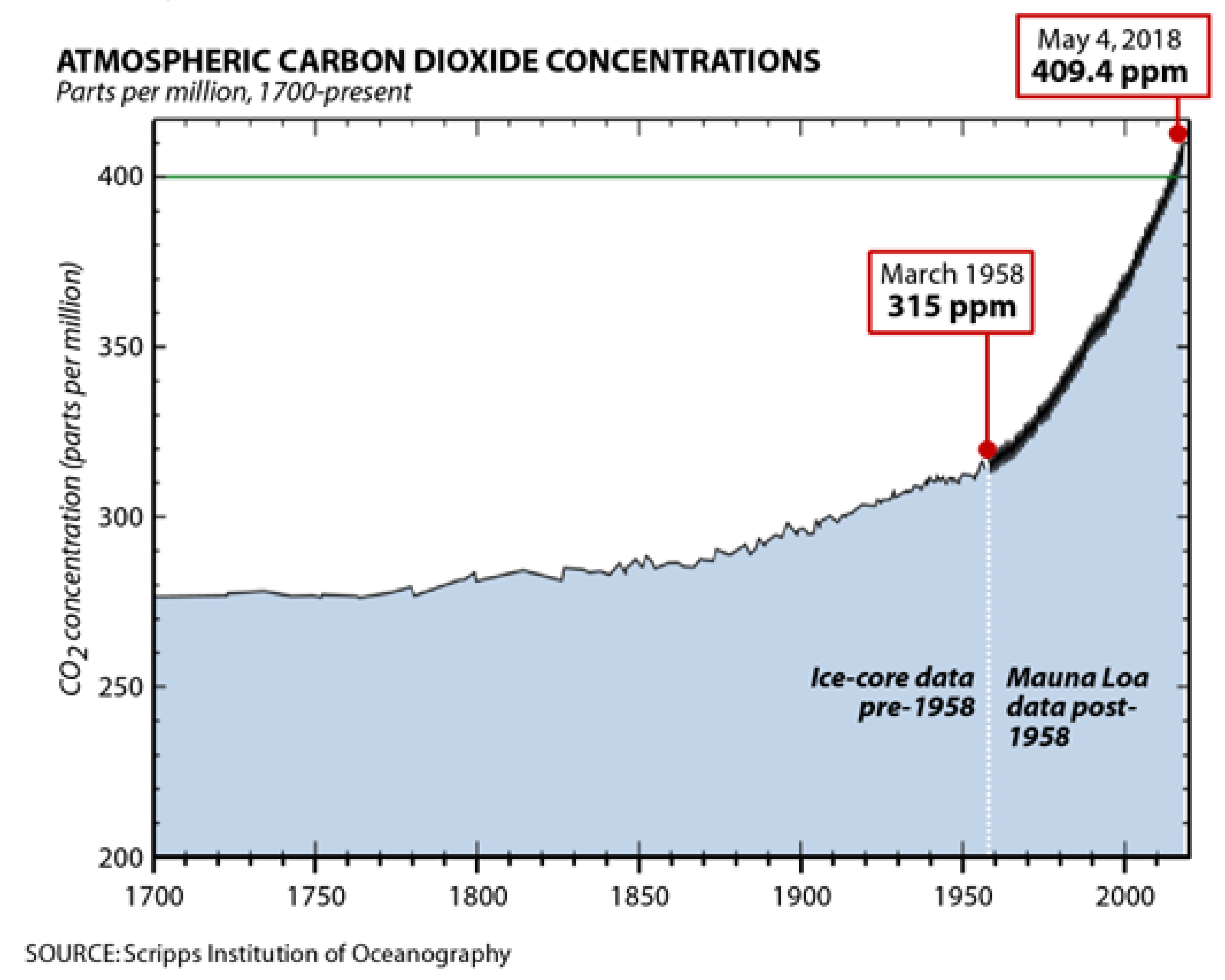
Development and evolution of organisms is generally strongly correlated with temperature. It should not be surprising then that increasing CO2 (which is synchronized with increasing temperature) is correlated with the increase in rate of evolution on Earth’s surface. However, it is probably unlikely that the CO2 will remain the main driver of temperature increase.
Extrapolating from Figure 21, from year 1850 onward:
which, for the concentration of 800 ppmv gives year T = 2075.
Note that the equation roughly corresponds to IPCC RCP8.5 (Representative Concentration Pathway 8.5) scenario. Both predict equal CO2 for the year 2100, however, RCP8.5 predicts 800 ppm to be reached sooner - in year 2066. RCP8.5 is considered the worst-case scenario and, at this point, still may be considered unlikely.
However, while replacement of coal and oil with other energy sources may eventually reduce human CO2 emissions, it is not reducing human impact on nature, which is generally not directly proportional to CO2 emissions, rather to energy (resources) consumption, which is growing as usual.
If the impact threshold is reached (point of no return), human emissions are completely irrelevant and positive feedback mechanisms will produce climate consistent with the RCP8.5 scenario. Studies are already confirming this[223].
Humanity may be [very] slowly abandoning the business of CO2 emissions, but, as proper cancer, it has not abandoned the unsustainable infinite growth policy.
Climate is a part of an eco-system, it evolves with the eco-system, and one cannot expect that disruption of eco-systems won’t impact climate. Since causality is relative, disruption of eco-systems can be interpreted as a precursor to bigger climate disruption, mass extinctions are always relatively synchronized with climate disruptions.
While humans may eventually reduce their CO2 emissions significantly, the rate of evolution should keep accelerating according to the equation and, regardless of the atmospheric CO2 (which may still be increasing even with 0 human emissions), the required pH minimum will eventually be reached.
Asteroid impacts, previously correlated with Earth’s graviton energy level changes, should start before the migration, increasing in frequency and energy with time. Although required energy for changes may be lower than in previous major extinctions, it should still be significant.
Lower requirement for energy from asteroids, natural earthquakes and volcanism, if real, may in part be due to the presence of effective anthropogenic equivalents (e.g., wars, nuclear detonations, drilling, etc.).
However, energy requirement primarily comes from the difference in graviton energy levels and these can be associated with mantle layers/discontinuities. Here, I assume that layers III, IV and V are the result of splitting of a major energy level - thus, the mantle has 4 major layers, although effectively 6 due to energy splitting. Note that the thickness of major layers is roughly doubling with depth. Since the energy requirement for excitation is decreasing with distance from the centre (reflected in decreasing thickness of 4 major layers towards the top) and assuming the current energy level is increasing with each major extinction, the energy requirement for excitation must be decreasing too.
Assuming interval between possible impacts is quantized proportionally to [the equivalent of] a 50 ppm CO2 increase (representing a quantum of energy), given the C1.1 equation, one can calculate potential years of impacts and correlate these with potential impactors, as shown in Table 25 for several concentrations. Evidently, there are good candidates among extinction causing asteroids in NEO (near Earth orbit) for calculated dates. Here, the 1866 Sisyphus is the impactor correlated with the 2nd order period of the Solar System oscillation (≈26 my). Note that the impactor in the last major extinction was larger (Chicxulub), making this consistent with the hypothesized decrease in required energy for development with time. Ryugu can then be interpreted as a 3rd order impactor, while Apophis is a 4th order one, albeit a bit larger from the expected average diameter of about 120 m for that order.
Note that a relative synchronization of multiple impactors of different order is expectable if order periods are harmonics, as hypothesized. Note also that the extreme size of Apophis for a 4th order impactor does not rule it out as the impactor. It is possible that Apophis will break into two smaller asteroids and only one part will impact the Earth. Another possibility is that Apophis should be interpreted as a superposition of impactors of different order (this, however, can be interpreted as the reason for breakup). If large scale gravitons are coupled to these asteroids, breakup could be interpreted as decoherence. Interestingly, year 2046 has been calculated previously for the end of the current 4th order cycle. Closest approaches of Apophis are in years 2029, 2051 and 2066. Year 2051 is relatively close to 2046 and a superposition of 2029 and 2066 in the form of an average gives a year 2047. A coincidence, or a signal that Apophis may indeed break into smaller parts and two parts will be absorbed, one in year 2029, the other in 2066, or there will be a single absorption in year 2051? However, one could argue that any year apart from year 2029 (the year of closest approach) is an unlikely candidate, as, according to calculations[227], Apophis was nearer Earth in the past than it will be in years 2051 and 2066 and nothing happened. But one could also argue that the probability for capture is a function of both distance and time, not distance exclusively. Assuming 50 ppm quantization is correct, close approach years 2029 and 2066 match exactly the calculated impact years, but even the year 2051 is not far away from year 2048 (year associated with 550 ppm). As for the calculated past approaches of Apophis, there are no such good agreements, except for the year 1907, which can be correlated with 300 ppm. That approach may be further correlated with the Tunguska event in 1908.
But should large scale gravitons be coupled with these asteroids? Possibly, if these asteroids act as relative triggers of energy level changes for the local Earth’s graviton. However, it is also possible that gravitons are not coupled to these asteroids at this time, rather, will be coupled prior to impact. In fact, the late coupling is probably required to put these asteroids in the collision course with Earth at the years specified in Table 25. The question then is where will these gravitons come from? Sources may differ, depending on the impact order, however, it is also possible that the source remains the same (e.g., the Sun), only the graviton energy differs between orders. Apophis may be even broken up by humans (which, if it does happen, I wouldn’t interpret as a non-coded event). Apart from the Sun, most likely other potential graviton sources may be Earth and the Moon. Temporary delocalization of the Earth’s graviton, for example, could drag the asteroid towards Earth with subsequent localization (not just the asteroid, it could drag all the junk humans have put in the orbit as well - but this depends on graviton dimensionality during collapse). One interpretation of this may be feeding, even if unconscious (what is feeding, if not acquisition and transformation of energy into suitable form for local use, e.g., body development) - similar to the unconscious or deeply subconscious feeding of standard embryos in a standard womb. Rather than involving local gravitons directly, this may involve emission and local absorption of large scale gravitational waves (hypothesized to travel/expand at or near 2.93 × 10⁶ m/s), but the effects are similar. Note that this kind of asteroid capture helps explain the relative periodicity of impacts - the near Earth visitors may occur at random intervals, but they are periodically captured (the periodicity may be similar to our feeding habits - we may not feed exactly at the same time every day, but we do eat every day, at least if there’s food available nearby). What’s interesting about this interpretation is that this could actually increase the probability for larger impacts, as larger impactors may be more likely to be captured (analogous to the big fish eating big prey). However, what actually is the appropriate size? Blue whales, for example, feed on krill, animals which are about 500 times smaller than them. An asteroid 500 times smaller than Earth is about 25 km in diameter. In any case, if the proposed mechanism of asteroid capture is indeed employed at times, some limits on size and distance should exist as well. Lower limit for size is probably not below 100 m. As for the limits in distance (range of capture), nearer approaches are certainly more likely to be within the range of capture. It is probably safe to assume that the approach of Apophis in 2029 is within that range (estimated distance of the approach is about 38000 km), but is it the right time? Generally, thus, all the predicted impact years should be questionable, especially if Apophis is not captured in 2029. Close approaches of Sisyphus, for example, are still about 15 million km away from Earth and Sisyphus was closer to Earth in the past.
Energy requirements also depend on the rate of development. It is not surprising then that the frequency and size of impacts is largest during early planetary development.
A relatively good news in all this is that there are no signs of potential 1st order impactors (which should be on the order of at least 100 km in diameter) in the near future. This may indicate that the end of the current 1st order cycle is millions of years away. On the other hand, considering the expected disturbances with the end of the current 2nd order cycle, situation can change.
In the previous major extinction, all of these impactors were probably bigger. As noted already, multiple impactors correlated with a single major extinction are likely. Some smaller impacts that can be correlated with the current extinction may then have happened already (e.g., the Chelyabinsk meteor and the Tunguska event).
Note 1: According to current models based on Newtonian mechanics or GR, none of these asteroids are on a collision course with Earth in near future. However, conventional models obviously do not account for the periodic disturbances of the system with the collapse/inflation of gravitons and emission/absorption of large scale gravitational waves.
As argued before (see, for example, chapters 9. The cycles and 14.3. Correlation with extinctions), there are good reasons to believe that courses of asteroids are altered at times of extinctions.
If these impacts are genetically coded at some level, as hypothesized, they should not be questionable, it is only the source and method of delivery that may be unknown prior to the event.
Note 2: Interestingly, there was an impact event on Earth at the time when 400 ppm CO2 was reached (Chelyabinsk meteor, ≈ 20 m diameter, 2013.), agreeing with hypothesized 50 ppm quantization and suggesting that, not only are intervals between impacts quantized, but that impacts may possibly be expected with every 50 ppm of CO2 increase.
However, if the events are generally correlated with the average ppm value given by the C1.1 equation, which gives year 2015 for 400 ppm, the 400 pm in year 2013 should be understood as deviation due to inherent uncertainty.
Assuming probability of correlation of these events with CO2 significantly increases once CO2 rises above background levels, the first event should have occurred at 300 ppm - the beginning of industrial revolution. Indeed, one such event had occurred at 300 ppm - Tunguska, 1908. Note that the Chelyabinsk meteor is the largest known body entering Earth’s atmosphere since the Tunguska meteor.
The equation gives year 1992 for 350 ppm. No meteors of comparable impact energy to the Tunguska or Chelyabinsk were recorded in or about 1992., probably eliminating highly energetic direct impacts on land area. If a stronger event did occur, it had likely occurred over the ocean, triggering large waves and possibly earthquakes. Interestingly, an 7.2+ magnitude earthquake and tsunami wave did occur offshore in Nicaragua in 1992. This earthquake is notable for the tsunami wave being unusually large (9.9 m high) for the strength of the earthquake (belonging to a group of rare tsunami earthquakes).
I do not believe, however, that the impact (assuming it happened) caused the earthquake. This was likely the effect of synchronization of events (synchronicity) - the tsunami was caused by the earthquake but it was amplified by the impact. The Earth is a living being and it would not be surprising it reacts, even if unconsciously, to incoming bolides and impactors (just like humans do) to some degree.
I have witnessed such synchronization myself - on 2019.03.07 I have observed a larger meteor burning up in the atmosphere exactly at the time of an earthquake in Hungary, its trajectory was, at least roughly, towards the epicentre or the hypocentre. It is even possible that Earth reacts to every possible impactor, although the reaction may be proportional to impactor energy and thus usually negligible.
Note that, due to enhanced relativity in causality on the scale of U1 gravitons, the reaction can happen some time before or after the impact.
Also interesting about the Nicaragua event is that it occurred at the time of my birthday (September 1st, local time) producing an obvious signal[234] for me. Based on my heavy experience in synchronicity (I’m experiencing synchronicity almost on a daily basis for years now), I could now interpret this as a confirmation that the meteor was indeed involved in this event (and I originally did), but I cannot claim high confidence in such interpretation.
Note that Nicaragua, Chelyabinsk and Tunguska impact sites on the world map can be connected with a straight line - a correlation suggesting that the next impact may also occur somewhere along this line (even the Chicxulub, Yucatan crater is close). This correlation is a form of synchronicity as well, which then increases the intensity of synchronicity correlated with Nicaragua and the associated impactor. Still, the effect on confidence is marginal. Additional, and stronger, evidence is needed for a highly energetic impactor in 1992.
Although there were no sightings of extremely energetic meteors over land in 1992, there was a notable incident in Uganda, where a large explosion and infall of 150 kg of material in the shower was recorded[235]. While such incidents may not be so rare, it is interesting that this event occurred only 2 weeks before the Nicaragua event.
Also interesting, and symbolic, is the fact that the last visit of the Halley’s comet to the inner Solar System occurred about the time when 350 ppm CO2 was first reached - in 1986., and the next time it will be close to Earth is 2061. - exactly at 650 ppm (calculated using the C1.1 equation).
On the other hand, the assumption of 50 ppm quantization may be wrong, a 100 ppm quantization does not require the impact in 1992 while still predicting Tunguska and Chelyabinsk (gives year 2040 for the next possible impact).
It is currently hypothesized that Tunguska event was caused by a large body which eventually escaped Earth’s atmosphere - it can thus be interpreted as a warning.
Given the fact that neither the Chelyabinsk nor hypothesized Nicaragua meteor did not directly impact land, it appears these too were warnings.
However, I do not interpret these as warnings. I believe one purpose of the atmosphere is to disintegrate incoming bodies to protect life during weak evolution. Without it the Chelyabinsk meteor would be called a meteorite. Tunguska asteroid close-by, however, would not leave any effect but the atmosphere might have caused the Tunguska asteroid to split. I thus believe that whatever caused the Tunguska event is destined to eventually hit Earth, the Earth might have just quantized it and spread over time with its instinct (manifested as atmosphere) to defend its surface life.
These recent events may then be interpreted as signals of things to come.
Note that Newton calculated year 2060 as the first possible year of the Day of Judgment (but what I interpret as the beginning of the end of the surface world, at least in one model), although allegedly he revised this year later to 2016 by the suggestion of others. His final decision to revise the year was, however, based on a signal. As he was doing calculations, large earthquake occurred, which he later interpreted as a signal that the year 2060 is wrong. This earthquake could be interpreted a signal, but he misinterpreted its meaning - a better interpretation, at least from the current perspective, is that earthquakes are to be expected at the end and may have a prominent role in it. Newton also calculated that the end cannot come after year 2344[236]. Interestingly, this can be correlated with the previously determined pH minimum (which should be reached sometime between ≈2040 and ≈2300, with earlier dates probably more likely).
The year 2016 is not there without a meaning for me too, it is the year [of the start] of my soul rebirth (transformation, or change of soul energy level) occurring at the age of 36±1 (here, margins may be interpreted as the spread of the transformation in time as it is not absolutely instant) of the incarnation[73]. The calculations of Newton are based on the writings in the Bible and one could certainly argue that these should not be taken into account. I, however, interpret it as a correlation that is increasing intensity of synchronicity here, increasing confidence, even if marginally. Note that year 2016 may indeed be the point of no return regarding the collapse of civilization at least[237], but some other tipping points may have also been reached about that year, associated with climate change and biodiversity loss.
Note also that the year 2016 is not far from the year 2015 (year associated with 400 ppm, per the equation), while year 2060 is not far from the year 2061 (year associated with 650 ppm, per the equation).
Note 3: Interestingly, at the time of the Chelyabinsk event, Apophis asteroid was in close approach. Considering that the composition of Chelyabinsk meteor seems to match the composition of Apophis surface (LL chondrite) a possibility does exist that the meteor broke off of Apophis and is thus a part of impactor energy splitting.
Note 4: The equation C1.1 is one variant of the universal equation for a pulse of strong evolution. That 800 ppm as the CO2 marker maximum was a good prediction can be confirmed with another variant (inverse) of the equation, one correlated with half-lives of elements:
where C1 = (T1) is the half-life of the element measured at time T1. The equation gives half-life of 0 at, or near, T = 2075, which is the year when CO2(T) is equal to 800 ppm (half-life however cannot reach absolute 0, suggesting that 800 ppm is an unrealistic marker in this interpretation). Just like in case of CO2 I do not expect for half-lives to follow the equation continuously (e.g., half-life might appear constant and then get reduced significantly in an instant). Generally, changes in decay rates should require sudden changes in properties of space.
One exception to this could be the half-life of 10Be, due to vertical entanglement with the local U1 system. If the Solar System cycles through 10(C-B-Be) in the 1st order cycles, a continuous precursor enrichment in 10B at a lower scale (U0) may be effectively announcing the state change of the parent U1 system (the Solar System).
For 10Be, incorporating the value from the most recent measurements (T1 = 2010, (2010) = 1.387 × 10⁶ y), the half-life equation is:
and it gives values in good agreement with previous measurements, as shown in Table 26.
* the value is not the initially published value, but the result of reanalysis/correction in 1972.,
† these values are discarded by scientific community, citing potential systematic errors
(based on the presumption of absolute constancy of decay rates).
All measurements agree well with calculated values, except for 1986 - if there were no flaws in measurement, this may be attributed to deviation due to cycling (similar to yearly fluctuation of CO2). Note, however, that measurement 1993 was done on the same SRM (Standard Reference Material) sample and discrepancy suggests one of these measurements is wrong.
If indeed the half-life of 10Be is decreasing as hypothesized, modern science has been effectively doing cherry-picking here - discarding results which do not agree well, or are in discrepancy, with latest measurements.
Given the current precision of measurements, a new measurement at this point in time which would agree with the calculation would be in discrepancy with measurements from 2010. and would thus confirm the hypothesis of continuous decrease of 10Be half-life with the extinction event.
Note that this effect on decay rates is temporary and significant only at the end of a cycle of general oscillation up to the 3rd order.
Note also that decay rates may not be always changing directly (affecting half-life) rather effectively (CR requires effective oscillation in particle decay, but these changes will not always be reflected in half-life of the element) - e.g., through spallation reactions.
However, also note that the measured/calculated strong decrease of 10Be half-life (with no associated apparent significant gravitational disturbances) can be interpreted as a consequence of relativity in causality. In that case, this decrease could be a precursor to real global change (across all unstable elements), announcing pending gravitational disturbance - collapse of the local gravitons. If 10Be half-life continues to follow the equation, collapse probably has to occur before year 2075.
Note 5: In the previous note it was assumed that half-life decreases fast and the equation allows it to eventually drop to zero (although, the compression of time implies that this state lasts 0 time - thus, effectively, half-life never becomes 0).
Another possibility, although unlikely, is that half-life cannot ever reach zero, even for 0 time. In that case, the equation might have this form:
This yields, for T1 = 1987 (C1 = 1.512 × 10⁶ y, CO2(T1) = 341.83707500861), results in Table 27.
where uncertainty in calculation is the scaled variation of CO2 (10 ppm).
Multiple extinction pulses may not only be plausible but necessary - first pulse would include asteroid impact(s) (possibly triggering additional ocean acidification and formation of the layer in the mantle), the other would provide new water/life, either by comets or asteroids. A third pulse in between might also be needed to trigger the (now acidified - CSF) ocean sink and, relatively, sterilize the surface (as noted before, all this is probably synchronized with magnetic field collapse, allowing surface sterilization by UV/gamma radiation).
Note that, if this is the last embryonic neurogenesis event of Earth, a collapse of Moon’s graviton probably should be expected. Remains of the Moon could then be the source of eventual impacts of cometary nature (dust/water/ice).
This is evident on Mars - as layers below the surface formed, magnetic field receded leaving the surface sterilized. Water froze and is now covered with dust. Thus, one can only expect to find residual and resilient bacteria within the upper crust of Mars.
Similar probably happened on Venus except water may have evaporated due to high surface temperature.
Nothing in nature is absolutely linear (although this approximation may be suitable during stages of weak evolution) and in these extreme events one can expect significant departures from linear relations (by multiple orders of magnitude) between phenomena.
Since these events are coupled with gravitational stresses of the Solar System one can expect temporary but significant increase in alpha and neutrino radiation (radiation flux induced by temporary collapse of a gravitational well associated with a large scale graviton - strongly affecting half-lives of isotopes).
One interpretation of changes in decay rates could be [inverse] time dilation due to scale change of gravitons, but what actually are the mechanics?
If this collapse is synchronized with the collapse of the magnetic field, increased incidence of cosmic rays will increase decays of elements but this is limited to surface and should not be interpreted as real, rather effective and limited, change in decay rates.
However, a mechanism for real changes does exist. Graviton of Earth must be entangled with static graviton neutrinos that form its space. Spin/scale change of the large scale graviton will thus be synchronized with spin/scale changes of these neutrinos. In equilibrium, when the gravitational well is full, these neutrinos are [most of the time] bound to standard atoms contained in [or bound to] the gravitational well of the maximum. Obviously, disturbance of these neutrinos (decoupling from atoms) will destabilize the atoms and induce decays.
Also note that these changes are synchronized with orbital changes of large scale maxima in the Solar System - which, like the decay rates, are accelerated during the pulse but return to normal after the pulse.
Due to dependence of the density of graviton neutrinos to the distance from the gravity source (density being generally inversely proportional to distance squared), it is possible that even orbital changes in eccentric planetary orbitals are synchronized with changes in decay rates, with some phase shift (in that case, graviton neutrinos directly affected are the static graviton neutrinos of the Sun’s space). However, there is no spin/scale inversion in this case and there will likely exist a threshold eccentricity required to produce significant effects (this can be experimentally verified with satellites in eccentric orbit).
In fact, this may have been detected already[239], and can also be correlated with oscillation of fundamental constants, such as G (as presented already).
Due to universal synchronization and restoration of previous equilibrium states it may be hard to detect strong pulses in the past. In fact, astronomical and geological observations, generally, probably will not reveal any deviation from constancy of decay rates. However, probably all records of cataclysmic changes should be interpreted as fossils of this elementary destabilization.
Thus, with such nature of changes (rapid excursions), the principle of uniformitarianism in this context may inevitably seem, but cannot be, valid.
Note also that most of emitted radiation will be lost to space for the same reason - temporary collapse of gravitational/electro-magnetic well, thus solving the problem of missing radiogenic Helium[240]. Due to conservation of momentum, significant loss of heavier atmospheric particles is not expected due to well loss, but can occur during the short exposure to solar wind.
The assumption of absolutely constant decay rates will not only produce incorrect ages but can result in misplacement of events on a geological timescale. Thus, inconsistencies in certain geological records can serve as indirect evidence to disruptions in decay rates.
Consider the neutrino pulse in Figure 22 - under the assumption of constant decay rates, 3 different fossil records A, B, C may give the following results:
- assuming non-isotropic space-time perturbation, such that fossil record A decay is not affected by the event at , the event at (associated with fossil record B) may appear to have happened before the event at (associated with fossil record A),
- in case decay rates of both A and B are affected, the distance of and to will be increased (time interval expansion).
One potential example of this are the late Eocene impact events. Here, two impact craters with diameters of ca. 100 km and 40-85 km (Popigai and Chesapeake Bay, respectively) are associated with extraterrestrial impactors, with the two events occurring within <25 ky of each other. Despite the large size of impactors, no isotopic anomalies or excursions were recorded across the impact horizons[241]. This is highly unusual, considering that the total energy involved is not much smaller than that of the Chicxulub impactor, assumed to be the primary cause of the disruptions leading to the Cretaceous-Paleogene mass extinction. However, climatic disruption did occur in the late Eocene some 100,000 years before the impacts[241]. Thus, this may indeed be an example of misplacement of events due to an asymmetric disturbance of decay rates.
Note that one reason for the existence of asymmetric effects is the conservation of relativity in causality or causal order, postulated in CR.
Neutrino flux can also be decreased indicating shortening (rather than expansion) of time intervals, although in this context the increase of the flux is expected.
Due to accumulation of effects over time, duration of fossilized events would apparently increase with time making older events seem longer in duration compared to more recent events. This is exactly the case with current fossil evidence of past carbon cycle disruptions.
In such case, the current rate of CO2 injection is probably not different from those in previous major extinctions (the fact that it is anthropogenic makes no difference).
If one assumes that the average period between extinctions is equal to the 2nd order oscillation period of the Solar System, in case of ideal synchronization, it is quantized by the 3rd order period of existence (Tx = 1.512 × 10⁶ years). In such case, assuming the period must be roughly 26 or 27 million years, the proper period is:
This is in agreement with the previously determined periodicity of impact cratering (25.8±0.6 × 10⁶ years)[217].
One can now assume that the CO2 injection within the Cretaceous-Paleogene (K-Pg) boundary (66.5 - 65.5 mya) is equal to the current injection (currently dominantly anthropogenic) and that increase of decay rates (effective compression of time, causing boundary to be significantly overestimated in duration) is induced within the boundary - with the start of the boundary corresponding to tA and its end to tC in Figure 22.
Assuming CO2 increased from 780 ppmv to 1440 ppmv (CO2 = 660 ppmv) in the period 66.5 mya - 65.5 mya (ti = 1 million years)[242], compression of time tc with each major extinction is:
where is the period of 660 ppmv of anthropogenic CO2 increase since year 1850 (assuming this is the start of the new boundary), calculated using (C1.1).
Such compression of time is easily achievable using C1.2. In example, for 10Be:
Half-life of 10Be decreasing by the above equation, reaches required time compression in year 2065, on day 66 of the year. Source code:(Fig.: getage.php +)
However, year 1850 as the start of the boundary may not be convincing and recent research shows CO2 injection of ∼250 ppm, not 660 ppm, within the K-Pg boundary, though this does not affect compression (tc) significantly (it makes it larger for a couple of decades at most).
Probably most likely start of the new boundary (end of Holocene) is year 2065 or 2066, which, with an increase of 250 ppm, gives year 2084 as the end, the same as in the previous assumption (1850 + 234 = 2084).
Number of 3rd order cycles of existence since Cretaceous-Paleogene extinction event (66 mya):
Decay rates may be affected by the cycle of any order, however, beyond the 3rd order, the effect is probably negligible. Here, thus, only 2nd and the 3rd order cycles will be taken into account (the effect is largest at the end of a 1st order cycle, however, that cycle is irrelevant in the current context).
Gravitational collapses during strong evolution pulses with a period of Tx years (3rd order period) may last only = 19.3 seconds, but collapses during stronger evolution pulses occurring with a period of Td years (2nd order) last longer (7 days should be the maximum to conserve structural stability, as calculated previously).
Synchronized with each large extinction, gravitational maxima of the Sun collapse.
This, may or may not - depending on interpretation (mass being shielded or not) and the current energy level of the outer graviton, result in the release of condensed energy beyond the Sun’s surface - effectively expanding the Sun. In any case, the amount of collapsed maxima should be inversely proportional to cycle order. Major extinctions are correlated with 2nd order cycles. At the end of such cycle, probably both the inner and outer maxima (or, large scale gravitons) of the Sun collapse temporarily.
Assuming [information about] the gravitational disturbance reaches the orbit of Mars at the time the gravitational well is restored (the collapse may be interpreted as the temporary change of energy level of the gravitons), with the disturbance travelling at the speed of light, time of increased decay radiation is, for a 2nd order cycle:
where rM is the distance of Mars from the Sun.
Now one can calculate time compression at the end of a 3rd order cycle (extinction pulse), , and with a stronger (2nd order) pulse, :
tc = cumulative compression of time ≈ 2nd order compression + 3rd order compression = 999766 y
= interval of collapse (disturbed decay rates) for a 2nd order cycle = 760.259 s
= interval of collapse for a 3rd order cycle = 19.3 s
Age of Earth is thus overestimated by:
giving the real age of Earth:
where = 4.54±0.05 × years.
If one assumes that Td (2nd order period) is the equivalent of 1 day of human embryo development, Earth is at the week 25 (GW25) of the gestation period (right at the beginning, in case of corrected age).
The GW25 marks the end of embryonic neurogenesis in humans and thus agrees with the suggestion of the final major extinction.
The current carbon cycle disruption (6th major extinction) will thus not span thousands (∼10000) of years as predicted by the assumption of constant decay, but possibly 234 years starting from year 1850 (∼10000 years of already passed Holocene extinction may be regarded as a precursor to the major event starting with the year 1850).
Note that this year corresponds to 950 ppm, as predicted by (C1.1).
The calculations above should be understood as the proof of concept, at least. The actual / ratio could be different in reality, however, probably not much. The chosen value for may seem arbitrary, but it is based on the assumption of entanglement between U0 and U1 scales. Since the period Tx (1.512 × 10⁶ y) is equal to the half-life of standard 10Be, the period is assumed to be equal to the half-life of 10C (19.3 s) - this should be the correct order of magnitude for the value at least. What is interesting about this value is that a wave/information travelling at the standard speed of light, after this amount of time, reaches the distance from the Sun exactly equal to 1/10 of the orbital distance of Mercury. Also interesting is the fact, that, with the same / ratio, but assuming is equal to the maximum value (7 days), the value of becomes such that the information travelling at the standard speed of light for the same amount of time reaches exactly 10 times the orbital distance of Neptune. Is this a coincidence, or does it suggest that the / ratio could be correct? For example, assuming is 10 times smaller than the maximum (7/10 = 0.7 days) or that is 10 times larger than 19.3 seconds, with the ratio conserved, information about the collapse reaches Neptune/Mercury, respectably, after the interval of time equal to . Note that Mercury - representing the innermost positive charge, and Neptune - representing the outermost negative charge, should be entangled according to the original hypothesis (equivalence of the Solar System with an standard isotope). Note that the same ratio can then be obtained if one assumes that graviton expansion, or information, travels at the U1 speed of light (2.93 × 10⁶ m/s). Restoration of the well once the information or graviton expansion reaches Mercury/Neptune does seem realistic as these are the particles that should be affected with the decay of 10Be/10C. One can now assume that the decay of the isotope has a chance to occur at periodic intervals (hence the probabilistic nature of half-life), correlated with graviton collapses, but it occurs only if the well (gravitational, on large scale) fails to restore before the information reaches the particle associated with the decay. Note that the proper superposition of orbital distances (relative to the proper event horizon) of Mercury and Neptune could give the orbital distance of the neutrino associated with the decay. A very interesting example of how one could learn about the details of the mechanics of certain unobservable phenomena on small scale by observing the large scale equivalent. Although, in this case at least, one may die while observing it...
Note that the 7 day interval can, again, be correlated with religion. One story that withstood the test of time and made its way into the Bible (under a different name though) is the story of a world-destroying flood, in the Epic of Gilgamesh (but similar stories, some of which are not based on this one, exist all over the world). In the story, raging wind, torrent, tempest and flood overwhelmed the world during 6 days and 6 nights, only to calm down on the 7th day. Exactly what can be expected in a major extinction correlated with graviton collapses and hypothesized planetary neurogenesis.
16.4.1. Magnetic Field Collapse and Tipping Points
As noted before, the 6th major extinction will likely include a decline of the Earth’s magnetic field, either as a temporary excursion (partial or global collapse), part of a complete reversal, or even a longer-lasting or permanent retreat. The Earth’s magnetic field is currently declining at an accelerated rate, which, when coupled with the rapid movement of magnetic poles, indeed could be interpreted as a sign of imminent collapse (although a temporary fluctuation cannot be excluded). The previously determined correlation of the 4th order period of general oscillation of the Solar System with past excursions (see chapter 9. The cycles) also suggests that, at least, a magnetic excursion is near.
If that is so, when will the collapse, partial or not, occur?
With no further acceleration of the decline the collapse would occur sometime beyond year 2100. However, such scenario is unlikely - a tipping point and additional acceleration is expected for a collapse.
The collapse should also be relatively synchronized with other impactful events, which, as I hypothesize, are correlated with the rate of evolution - which is currently correlated with the rate of atmospheric CO2 increase. With the assumption of tipping events occurring with every 50 ppm increase of CO2 (or the equivalent energy increase), per the equation C1.1, one obtains the following years:
- 2029, 2040, 2048, 2055, 2061, 2066, ...
Thus, the magnetic collapse should not occur before the year 2029 (or, 450 ppm CO2) and most likely not after the year 2066. per the calculation done in 9. The cycles, it’s most likely to occur sometime about 2046, however, it a full reversal is imminent, it may be preceded by multiple partial and/or temporary excursions, perhaps even with the first one occurring about the year 2029.
Tipping Points
It has been postulated in CR that energy exists at different scales. In some interpretations this is the simultaneous existence of one and the same energy (implying any difference is in the metric and/or the frame of reference), in another, the equivalence is more relative. In any case, however, entanglement exists between scales. The transition between energy levels on one scale can be interpreted as discrete, on the other continuous. From our perspective, the increase in (energy) is continuous and is coupled to some proportionally increasing values (e.g., temperature), however, apart from the continuous changes, correlated abrupt changes can happen as well, and these abrupt changes can be interpreted as a discrete transition from one stable state to another. Energy levels generally follow exponential progression, the , or atmospheric energy, is rising exponentially as well. Is it possible that the amount of energy correlated with an increase in 50 ppm represents a discrete quantum of energy in this context and the transition from an energy level (relatively stable state) to another then requires an amount of energy that is an integer multiple of that quantum? Evidently, it is possible, although the exact value of the quantum may be 100 ppm (as noted already) but it may also be smaller than 50 ppm (e.g., 25).
The question is, what kind of tipping points do the calculated years potentially represent?
As noted already, Tunguska event occurred at 300 ppm, Chelyabinsk occurred at 400 ppm and a fairly large asteroid (Apophis) will at least get extremely close to Earth in the year 2029, when the equation predicts 450 ppm. The equation gives 400 ppm for 2015/2016, which may have been a tipping point on some levels (for example, 2016 was the hottest year on record until 2023, and a rapid growth of atmospheric methane was observed at the time[244], some claim a tipping point regarding civilization collapse at the same time[237]). Thus, good correlation exists with asteroid impacts and there are signs of correlation with tipping points of different nature. It is possible then that even the magnetic field collapse would be synchronized with this.
Since the energy required for transition between energy levels decreases with the increase in level, the temporal distance between tipping points should be decreasing as well. Assuming Tunguska and Chelyabinsk events represent adjacent energy levels (and assuming hypothesized transition occurred), the next transition should require less than 100 ppm, and the most likely value is probably 50 ppm, giving year 2029 for the tipping point. Interestingly, the current solar cycle is expected to end about the same time - when the solar activity should be at the minimum and at half-point between reversals. This may not be relevant, however, as noted before, magnetic excursions and reversals on Earth may be highly correlated with the changes in the Sun’s magnetic activity. No significant mass ejections are expected at the cycle end. If the magnetic field collapse is correlated with mass ejections, it probably should be correlated with the solar cycle maximum, and of the obtained years, the next closest year that could be synchronized with such maximum is the year 2048, or about the time when 550 ppm [energy equivalent] is reached.
Note that the calculated years should be interpreted as probability maxima, correlated events should occur about the predicted year, may not occur exactly in the predicted year.
Of course, due to a small dataset, confidence here is not very high. Additional research (or more time) is needed to confirm this hypothesis.
16.4.2. Sea Level Changes and Migration
Assuming high similarity in neurogenesis between scales, planetary neurogenesis requires transfer of differentiated progenitor cells to subterranean world, into designated mantle layers. Therefore, a passageway would have to exist somewhere, connecting the surface with underground tunnels leading to such places. These tunnels may be long-lived or re-created as needed. The passageway on the surface, however, is unlikely to be open all the time. It is a relative equivalent of a mouth and living beings generally do not keep their mouths open all the time. Those who do not communicate verbally, may open their mouths only at feeding time.
Note that cultivated cells/proteins on the surface can certainly be interpreted as food (this is the case for migrating cells in standard embryogenesis as well). Everything that becomes incorporated in the body (whether during development or in adult stage of the host) can be interpreted as food. And it is not unusual for the individual quanta of that food to be many orders of magnitude smaller than the organism feeding on them. Consider whales feeding on plankton. Now, what could whales evolve into if they could evolve further? Probably an organism cultivating food on its surface. The food (e.g., something evolved from plankton) takes energy from the environment to grow and multiply. Once certain mass is established, the host stimulates the food quanta to migrate towards the mouth. By the time they arrive, the mouth is opened and they are further stimulated to go inside. Once the food is digested (which may or may not be necessary) and incorporated into the body, the waste products are expelled through another opening, or pores on the body. At least some of this waste could then be used as fertilizer on the surface. If waste is expelled at the time critical mass of food on the surface is reached, the waste itself could serve as a stimulant for migration of food towards the mouth. The benefit of cultivation of food on one’s surface is that no mobility is required. Thus, the energy requirements for life are significantly lower (energy is used solely for maintenance of introversion and intra-species communication). What about reproduction? No reproduction is needed if the population has reached cultivation peak. In other words, evolution has reached its endpoint or evolvability maximum (effective local goal), where the evolved organism may represent, for example, a neuron cell equivalent or an atom equivalent. This does not imply there is no death, such organisms may be regenerated or re-evolved when necessary. In another interpretation, the organism has reached a relative perfection, where further sexual recombination and natural selection would have a low benefit to cost ratio (which is obvious if all members of the population are pretty much identical relative to their function in the environment).
By that interpretation then, Earth is a perfect organism, and so is an atom.
Scaling the largest neuron cells to Earth size, the neural tubes (and possible the surface entrance) must have a radius of at least ≈ 250 metres to allow sequential cell transfer. However, parallel transfer of multiple cells is certainly more plausible - a radius on the order of 104 m or more. If the entrance to the interior is a relatively permanent feature (e.g., representing mouth equivalent) then it must be protected when unused.
The only location where this area could remain hidden (protected) and isolated when unused is probably Antarctica (even if the opening is closed, the additional layer of ice doesn’t hurt, it provides additional protection). Ice melting is then required to expose this location but likely also to raise the sea level as the ocean represents the CSF, the fluid that should flow into the tunnel eventually.
I have assumed humans, in addition to other animals, represent progenitor neural proteins. Even if it may be unlikely that living humans will be migrating deeper into the interior, rather recipes required to reproduce them (DNA), the sea level still would have to be high enough to flow into the tubes and pick up the [cell equivalents containing] viable human genomes. However, even if all the ice melts, depending on the elevation of the entrance this may not be enough. There are three solutions:
- additional water comes from the deep and/or from space,
- land depression,
- cataclysmic flooding, correlated with sudden changes in angular momenta of the Earth’s crust.
The most likely outcome is probably a superposition of these solutions. As noted before, with climate changes (and possibly nuclear war) Antarctica’s habitability will be increasing while the rest of the world is decreasing habitability. Biomass destined for migration (including people, or hybridized people[245]) will be thus lured or guided (e.g., by certain fields of potential) to Antarctica prior to migration.
Note that the collapse of the Atlantic meridional overturning circulation (AMOC) would significantly decrease temperatures in the Northern Hemisphere while, at the same time, it would further accelerate warming in the Southern Hemisphere, particularly about Antarctica. Apart from increasing storms, flooding and decreasing temperatures in Europe and North America (where, in the east, it would also raise sea level), the collapse would severely disrupt the rains that billions of people depend on for food in India, South America and west Africa. Thus, AMOC collapse would significantly increase habitability of Antarctica while significantly decreasing habitability elsewhere. Thus, this event is likely scheduled to materialize.
Studies are showing up suggesting AMOC is likely to collapse this century. A recent one predicts collapse sometime between 2025 and 2095[246], with probability maximum at year 2057. That study has been heavily criticized due to reliance on many assumptions, however, a more recent study with a different approach and increased reliability produces a similar result, estimating a mean tipping time at 2050, with a 10-90% confidence interval between 2037 and 2064[247]. Note that the year 2050 is very close to the one of the here calculated potential tipping points (year 2048/2049, or 550 ppm CO2 equivalent).
Increased levels of radiation (e.g., through a nuclear war, magnetic field anomalies) could also have a role in migration of biomass to Antarctica. Magnetic field is currently decreasing strength while tensions between US/EU and China/Russia are high and have been rising lately.
In standard embryogenesis, migration of cells can be stimulated by excretion of extracellular matrices (various cell products).
Here, one equivalent factor may be hydrogen sulfide (H2S), a highly toxic and unpleasant gas, which had a role in at least some past major mass extinctions. For example, natural gases (incl. hydrogen sulfide) leaked from deeper reservoirs in the Arctic could be carried by disturbed polar jet streams towards the equator, stimulating life to migrate south. Indeed, the increasing accumulation of Sargassum seaweed[248] on the shores of the Caribbean, America and Africa could be interpreted as a precursor to larger hydrogen sulfide emissions (the Sargassum is releasing H2S as it rots).
If environmental pressure is required to stimulate migration, a major extinction may be interpreted as a side-effect of migration induction, or a result of filtering - which can also be interpreted as natural selection. Is it a selection of most intelligent, most adaptable and/or most easily manipulated? In any case, those who do not migrate, lack intelligence or adaptation capabilities, are probably those who go extinct and will appear in the fossil record. If intelligence is selected for migration here (effectively, or whatever the interpretation), it is then quite possible that high intelligence has evolved, or has been cultivated, multiple times on Earth.
Assuming the migration will indeed happen this century, rise in atmospheric greenhouse gases seems unlikely to produce adequate rise in temperature required to melt all ice in the predicted short time-frame (≤2066). Thus, different mechanisms may be responsible to induce significant breaking and melting of ice sheets. In addition to greenhouse gases, geothermal sources are likely. Melting can also be accelerated by asteroids, but also by advanced alien species from the deep.
However, if time indeed gets effectively compressed (with temporarily increased decay rates of elements), radioactivity itself could contribute to melting. Assuming that the increase of decay rates of hydrogen and oxygen in water molecules doesn’t produce significant effect (hydrogen probably shouldn’t be affected at all, and the effect may be negligible for all stable isotopes), required radioactivity (heat) may be produced by less stable isotopes trapped in ice or by elements in the crust below it.
Note that a significant amount of sea level rise has been baked in already with the increase of CO2 from pre-industrial 280 ppm to present levels (≈410 ppm). The estimates are study-dependent (some are analyses of recent glacial-interglacial fluctuation, others of individual past events with different CO2 ranges) and range from 10 - 40 metres. The relationship is not linear and may go roughly like this:
- with in the range 200 - 400 ppm, sea level rise baked in is 26 m per 100 ppm of ,
- for 400 - 600 ppm, 13 m rise per 100 ppm ,
- 600 - 800 ppm, 4.3 m rise per 100 ppm .
This would then result in 65.8 m total sea level rise, baked in with CO2 rising from 280 ppm to 800 ppm.
Conventional Potential for the Faster Melting of Ice and Magnetic Field Migration
The rate of melting of interior ice on Antarctica generally depends on two heat fluxes - flux between the ice sheet and the atmosphere and the flux between the ice sheet and the base (geothermal heat flux).
Melting of ice sheets and erosion of land below are decreasing pressure on the rock and magma below. This should increase magmatism/volcanism and result in a positive feedback. Indeed, studies show a rapid increase in volcanism with the melting of ice caps at the end of the last ice age[249]. But how rapid can it be?
Recent measurements show that geothermal heat flux is bigger than expected but still low, lower than , on average[250]. Much bigger fluxes exist on Antarctica at the vents of subglacial volcanoes where they can be as high as . If such volcanism would spread all over Antarctica (average heat flux of ), all ice could be melt in about 760 years (without taking into account melting caused by atmospheric heating). At the moment, however, there are no signs of this happening (although this could change with the predicted global increase in volcanism, the signs of which may be here already[251]).
On the other hand, considering atmospheric heat flux alone, if the average temperature in Antarctica interior would climb by C (from -C to C), 40-50 years would be enough to melt all ice. Is this possible in the short-term? Well, this is exactly what happened on 2022.03.18 at Concordia Station[252] - temperature measured was a record high -C, about 43. higher than the median average for that day of the year.
Others report a temperature of -C, claiming C higher than normal[253]. Not 43., but close.
Similar was measured in Vostok, and these places are the coldest places in Antarctica. Is this the signal that yearly average of C could be reached in the short-term? I wouldn’t be surprised. However, melting of all ice is not required for the migration to Antarctic lava tubes. What is certainly required for this is a sufficiently large area to contain the biomass destined for migration. Before the migration to lava tubes, settlements may form on the surface. This may be an area with a significant geothermal flux. And the Earth’s magnetic field, which will become fragmented and weak generally, may have a significant dipole component concentrated in this area for some time. Depending on the sources of the magnetic field and how actually it is generated, it is possible that magnetic field does not collapse simultaneously everywhere. Magnetic shield could be thus active on Antarctica for some time after the northern areas lose protection. One possibility is the local establishment of a circumpolar current of ions (or gyres of ions) which would sustain the local magnetic field (similar to the geodynamo in the core). If the metal enriched circumpolar magma ring would form simultaneously with the decline of the magnetic field, the magnetic field would induce currents in the ring which would then create magnetic fields on their own. These fields could be sustained for some time even after the original (global) field declines to the interior. In this case, the currently existing oceanic circumpolar current could be interpreted as a precursor of such current. Note that ice on Antarctica does melt more at the edges of the continent rather than deeper in the interior. This decrease in pressure at the edges could help to establish the circumpolar ring of magma (which could then further help in melting of the ice).
Note that the entire process could be correlated with the energy level changes of the Earth’s large scale graviton(s), which may include excitation of the dipole (or one of its components) as well - increase of the dipole offset and its localization near the south pole. Since graviton energy level changes are further correlated with asteroid impacts, the impacts could contribute to the formation of the ring-like magmatism/volcanism as well.
In the process, a circumpolar ring of ridges on the crust surface could be formed, similar to the current mid-ocean ridges. And, similarly to the current creation of oceanic floor at mid-ocean ridges, new oceanic crust could be formed here as well, flowing radially inward and outward from the ring. If the magnetic field would be changing polarity during this process, a parallel circular stripes of the alternating magnetic polarity would be fossilized in the magnetite crystals as the lava cools. Now, if the planetary neurogenesis is not exclusive to Earth, rather common in terrestrial planets (as hypothesized, only temporal/spatial scales and rates of evolution differ) and possibly also moons of outer planets, the remnants of these stripes could be present even today on some of these bodies. Indeed, such remnants have been found on Mars[254].
Note that, if this volcanism has covered the entire planet or almost the entire planet (as evidence suggests[255]), any traces of past life that existed prior to migration must be buried below. Since the newly formed crust is thinnest at the north pole, this is where any potential search for this past life should probably start (alternative are the exposed deeper regions).
Note also that such extremely large resurfacing of material would hollow out extremely large tunnels below the surface. These would then probably represent neural tubes, but also could be reused as a habitat by life that remains on surface after the neurogenesis event, or even extraterrestrial visitors.
It is possible that the magnetic field on the south pole is sustained for millions of years, perhaps for the duration of another 2nd order cycle (about 26 million years). In that case, the hypothesized migration to mantle layers may not occur during the current event, rather in the next one, with the current event including only the surface migration and concentration of biomass on the south pole. However, I find that unlikely. In any case, if this magnetic field will be sustained for longer time, some life will probably remain on surface during that time (possibly the neutral, non-migrating/non-diverging individuals).
The Creation of Deeper Tunnels
By the theory, large scale gravitons (probably inflated from smaller scale) should be commonly involved in the formation of stars and planetary bodies. The inflation (or initial over-inflation followed be deflation and stabilization at the new energy level) of a graviton and dark matter associated with it is relatively synchronized with the clumping of real mass (ordinary matter) and makes the process of formation much faster and possible even in cases of strongly diluted real mass (like in the Kuiper belt of the Solar System, for example).
Given the generally torus-like shape and rotation of gravitons, concentration of mass is not isotropic.
Mass in planetary bodies should then be differentiated not only vertically, but horizontally as well, with lower density at the poles and possibly even with tubes (tunnels) connecting poles of large scale gravitons, or different energy levels in case of a single oscillating graviton (although these tunnels in terrestrial bodies would have to be eventually filled with fluids to ensure stability).
Note that Earth’s gravity is greater on the poles, but not as much as would be expected for either simple compression or redistribution of material. Density does seem to be somewhat lower at the poles. Are there tunnels below? Long-lived tunnels, except near gravitons, seem unlikely due to increasing pressure with depth, however, fluid density should be increasing with depth as well. High polarization and angular momentum of the wall material (or the fluid) can increase the stability of such tubes but this is not expected for the walls in terrestrial bodies (fluid flowing towards the centre would, however, possess an angular momentum). Long term stability could be ensured with appropriate density of energy levels and relatively frequent oscillation of large scale gravitons as this provides multiple density maxima. Lateral density gradient (with increasing density away from the pole) also decreases pressure on the tube and such gradients are likely for rotating bodies (note that Earth rotated much faster during formation). Otherwise, tunnels may be only periodically recreated (fluids remelt). I suspect that on bodies like Earth the fluids involved should be [salty] water and magma, with dominant fluid probably depending on the pole. Land should be depressed at the entrance where water is involved, however, it may be elevated on the pole where magma is involved. Interestingly, the subglacial topographic depression in Antarctica known as Wilkes land anomaly (elsewhere hypothesized 480 km wide impact crater, which would make it the largest impact crater on Earth) was directly antipodal to Siberian Traps (largest known volcanic event in the last 500 million years) during the Permian-Triassic boundary (Siberian Traps are considered to be the primary cause for the Permian-Triassic extinction, largest mass extinction on Earth).
Interestingly, the Siberian Traps may not be the only large scale phenomenon the Wilkes anomaly was antipodal to over time.
The 31 km wide Hiawatha structure on Greenland, hypothesized to be an impact crater, seems to have been antipodal to Wilkes anomaly at the time of the hypothesized impact (estimated to have occurred about 58 million years ago[256]). However, rather than being directly correlated with Hiawatha structure, Wilkes may be directly correlated with the creation of the Iceland hotspot (likely a mantle plume effect), which was located beneath Greenland at the time[257] and was responsible for the strong wide-spread volcanism (comparable to Deccan Traps) occurring there some 60 million years ago (Vaigat formation).
Currently, however, the Iceland hotspot is antipodal to the Balleny hotspot (Balleny islands), which may not be correlated with a mantle plume[258].
It is questionable whether impacts alone can cause significant igneous activity on the other side of the planet (although they can certainly cause earthquakes and can energize existing activity). However, the recreation of tunnels with graviton oscillation should create such phenomena at antipodal locations - depression on the side of water entrance/exit, bulges or traps at the side of magma expulsion (masking the depression). If Earth is modelled as a living being, different products on entrance and exit are expected. As tectonic plates move with time, the locations on the surface should move as well. I believe that all major mass extinctions are correlated with recreation of the tunnels. The Siberian Traps are already considered to be the result of a mantle plume which effectively is a temporary creation of a tunnel between the planet’s core and surface through which magma flows upwards. Antipodal volcanism is common to large craters of the Moon and Mars[259] and there are other examples of antipodal relationships on Earth involving large igneous provinces and hotspots (Yellowstone, for example, is antipodal to French Southern and Antarctic Lands). All of these may be correlated with oscillation of large scale gravitons and associated temporary recreation/reactivation of tunnels. In fact, deep mantle plumes may not be possible without it. As noted before, energy level changes cannot be absolutely spontaneous and large impacts can be interpreted as relative triggers of energy level changes of large scale gravitons. If graviton is, at the time of impact, oriented in such way that its axis of rotation is aligned with the impact site, and this should be likely at least for impacts occurring near the poles (possibly nearer magnetic ones if these are present), then the impact can be correlated with antipodal volcanism. In that case, the seismic energy generated by the impact further stimulates the flow of fluids through the tunnels, increasing the effect on surface (note that impacts do create chimneys of stress connecting the impact source with the antipodal location[260]). Generally, however, impact sites may not be aligned with the graviton axis at the time of impact and the magnitude of extinction then should be proportional to the alignment. The exceptional magnitude of Permian-Triassic extinction thus can be explained as a result of unusually high alignment.
If there are multiple gravitational maxima in the mantle, the lateral pathways in the core-mantle heat convection cells must be branching, corresponding to the number of maxima. Thus, plate tectonics may be present in multiple places, at different depths, in the upper mantle as well.
2025.01.24
Recent research goes in favour of this hypothesis[261]. The subduction of tectonic plates may not go as deep as previously thought. Deeper seismic anomalies previously associated with the subduction/recycling of surficial plates may rather be associated with different tectonic systems (potential habitable zones) at different levels of the mantle, as hypothesized above.
In fact, I suspect that surficial plate tectonics is only active during embryonic development, and possibly, in a limited way, during adult neurogenesis in mature planets (assuming it does happen on the surface).
In any case, the transfer of organics into the deep with the influx of salty oceanic water may be synchronized with the antipodal expulsion of magma and/or greenhouse gases. This expulsion would probably be methane dominated (which, however, would quickly oxidize into ) - explaining the dominance of in the atmospheres of Venus and Mars. Methane is already seeping from the depths in the Arctic - which could be interpreted as a precursor to this main event.
Interesting, in this context, is the previously hypothesized creation of a ring of fire at the south pole in the 6th major extinction. Here, lava spreading inwards could accumulate on the surface, but if this is indeed building of new crust it should include the subduction of the crust near the centre (which would be, by the hypothesis, also a magnetic pole). This material would be subducted in a gyrating fashion and would carry water with it as well. This can be interpreted as a creation/opening of the central tunnel leading to the deep. Conventionally, however, this process would occur slowly, over millions of years. Suppose, however, that the localized magnetic field is extremely strong and that flowing crust is in the form of magma. Superposition of water and magma would differentiate (subducting material would be layered). If vacuum exists in the deep (possible with multiple gravitational maxima), the pressure difference could further speed up the process (depending on conditions, this could allow even for the transfer of air). Multiple gravitational maxima in the Earth’s interior would ensure that differentiation is conserved. If vacuum exists, however, it is not required for the material to flow down differentiated, it can be differentiated in situ (e.g., through evaporation of volatiles). Differentiated transfer is only required in case it includes a transfer of biomass and structural integrity of that biomass has to be preserved. Now, if plate tectonics on the surface stops, it could still be active deeper in the mantle - the plates would simply cycle between different discontinuities (assuming plate tectonics is required to preserve life). Note that life in the interior does not require magnetic fields for protection and conservation of the atmosphere. It has a passive shield in the form of solid matter. Progression towards passive and more energy efficient solutions is probably expectable for the progressive evolution/development of a lifeform.
But is this type of transfer limited to the final major extinction? Probably not. Difference may be in the entrance points, extent of volcanism and the magnetic field (which may not lose global presence in other extinctions).
16.4.3. Analysis of Past Extinctions
Here, past extinctions are analysed for periodicity, with incorporated corrections due to previously calculated time compression with pulses of decay rate changes.
Periodicity is tested using circular spectral analysis[262] of a couple of datasets, which all give similar results.
Data is grouped into energy levels corresponding to the extinction magnitude (5 - major extinctions, 4 - minor extinctions, 3 - other extinctions, 2 and 1 - potential extinctions).
The Method
In the circular model of periodicity a time line is wrapped about a circle, the circumference of which represents a trial period. For each occurrence, a unit vector from the origin is calculated. If periodic, the series will tend to form a cluster at one point on the circumference when the correct trial period is used. Here, angular location relative to (present) gives the phase ().
Ages of individual events () are transformed to angles (, ) for each trial period P:
where R is the mean vector magnitude (normalized measure of goodness of fit). The phase shift () is calculated as follows:
Dataset 1
Extinction events in dataset 1, grouped into energy levels and calculated corrected ages for these events, respectively, are shown in Table 28.
Maximal R was obtained for a period P = 25.92 My (million years), with a phase of 9.355 My.
Dataset 2
Here, a larger dataset from a single source was used. Maximal R reveals a period P = 26 My, with a phase of 8.617 My.
Table 29.
Extinction events dataset 2, source: .
| energy level | extinction events [mya] | extinction events (), age corrected [mya] |
|---|---|---|
| 5 | 66, 201.4, 251.9, 372.2, 445.2 | 61.986, 190.308, 238.041, 352.461, 421.348 |
| 4 | 37.8, 145, 259.8, 306.7, 419.2 | 36.206, 136.774, 245.793, 289.975, 396.744 |
| 3 | 11.6, 93.9, 183.7, 228.5, 272.3, 423, 427.4, 485.4, 500.5 | 11.402, 88.465, 173.88, 215.987, 257.12, 400.469, 403.82, 458.929, 473.782 |
| 2 | 113.1, 168.3 | 107.344, 159.702 |
Extinctions and the result of spectral analysis are shown in Figure 24.
Dataset 3
Previous datasets do not take into account possible splitting of energy levels. Here, an even larger dataset is presented which shows possible energy splitting and how this, when not accounted for, causes lower confidence in calculated P.
Table 30.
Extinction events dataset 3, source: .
| energy level | extinction events [mya] | extinction events (), age corrected [mya] |
|---|---|---|
| 5 | 66, 201.4, 251.9, 372.2, 445.2 | 61.986, 190.308, 238.041, 352.461, 421.348 |
| 4 | 37.8, 145, 259.8, 306.7, 419.2, 514 | 36.206, 136.774, 245.793, 289.975, 396.744, 486.084 |
| 3 | 11.6, 93.9, 183.7, 228.5, 272.3, 423, 427.4, 485.4, 500.5, 541 | 11.402, 88.465, 173.88, 215.987, 257.12, 400.469, 403.82, 458.929, 473.782, 511.664 |
| 2 | 113.1, 168.3, 330.9 | 107.344, 159.702, 312.804 |
| 1 | 295, 346.7, 393.3, 467.3 | 279.448, 328.357, 372.239, 442.101 |
Here, for R = 0.413, obtained P = 22.493 My, phase 15.603 My.
Dataset 4
Here I hypothesize that deviations from P are the result of energy splitting into smaller events which when grouped properly would fit on P intervals.
The dataset is the same as dataset 3, except the hypothesized splittings (circled extinction pairs in Figure 25) have been grouped into a single event, simply by using arithmetic mean age of the pair.
Table 31.
Extinction events dataset 4.
| energy level | extinction events [mya] | extinction events (), age corrected [mya] |
|---|---|---|
| 5 | 66, 201.4, (251.9+259.8)/2 = 255.9, 372.2, 445.2 | 61.986, 190.308, 241.967, 352.461, 421.348 |
| 4 | 37.8, 145, 306.7, (419.2+423)/2 = 421.1, (514+541)/2 = 527.5 | 36.206, 136.774, 289.975, 398.619, 499.361 |
| 3 | 11.6, 93.9, (183.7+168.3)/2 = 176, 228.5, (272.3+295)/2 = 283.7, 427.4, (485.4+467.3)/2 = 476.4, 500.5 | 11.402, 88.465, 166.304, 215.987, 268.346, 403.82, 451.053, 473.782 |
| 2 | 113.1, (330.9+346.7)/2 = 339 | 107.344, 320.78 |
| 1 | 393.3 | 372.239 |
Figure 26.
Dataset 4 - extinctions (left), spectral analysis (right).
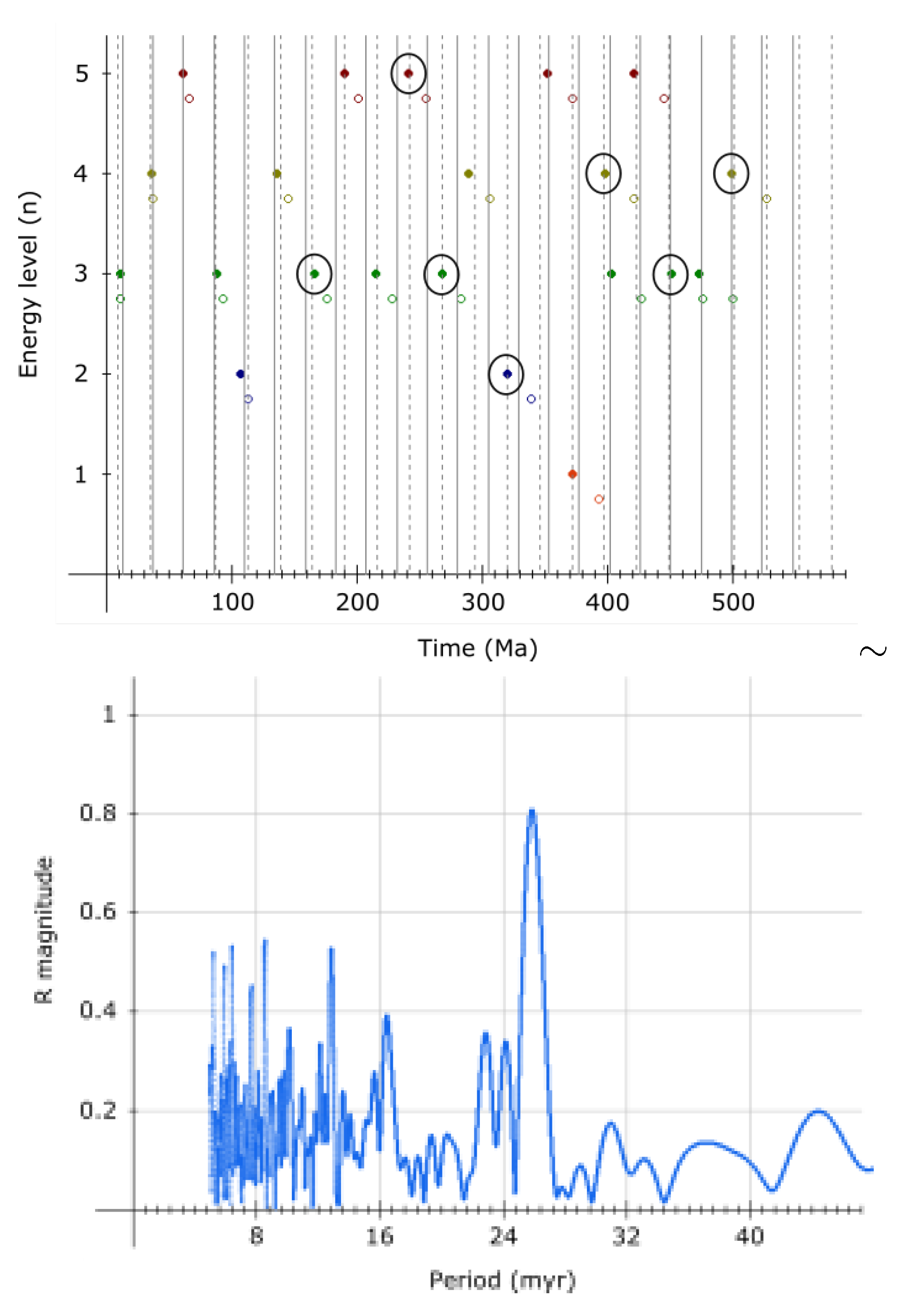
The R peaks at 0.807, corresponding to P = 25.89 My, very close to one obtained from dataset 1. Phase is 9.55 My.
Dataset 5
Here dataset 4 is modified with the assumption that splitting occurs in all events, thus, in addition to previously grouped events, the remaining non-grouped events have been grouped with adjacent boundaries.
Table 32.
Extinction events dataset 5.
| energy level | extinction events [mya] | extinction events (), age corrected [mya] |
|---|---|---|
| 5 | (61.6+66)/2 = 63.8, (199.4+201.4)/2 = 200.4, (251.9+259.8)/2 = 255.9, (372.2+382.7)/2 = 377.5, (443.8+445.2)/2 = 444.5 | 60.81, 189.333, 241.967, 356.687, 420.648 |
| 4 | (33.9+38)/2 = 36, (139.4+145)/2 = 142.2, (306.7+314.6)/2 = 310.7, (419.2+423)/2 = 421.1, (514+541)/2 = 527.5 | 34.431, 134.998, 293.926, 398.619, 499.361 |
| 3 | (11.6+13.8)/2 = 12.7, (89.8+93.9)/2 = 91.9, (183.7+168.3)/2 = 176, (228.5+237)/2 = 232.8, (272.3+295)/2 = 283.7, (427.4+430.5)/2 = 429, (485.4+467.3)/2 = 476.4, (497+500.5)/2 = 498.8 | 12.502, 86.49, 166.304, 220.213, 268.346, 405.395, 451.053, 472.107 |
| 2 | (113.1+126.3)/2 = 119.7, (330.9+346.7)/2 = 339 | 112.87, 320.58 |
| 1 | (387.7+393.3)/2 = 390.5 | 369.489 |
Figure 27.
Dataset 5 - spectral analysis
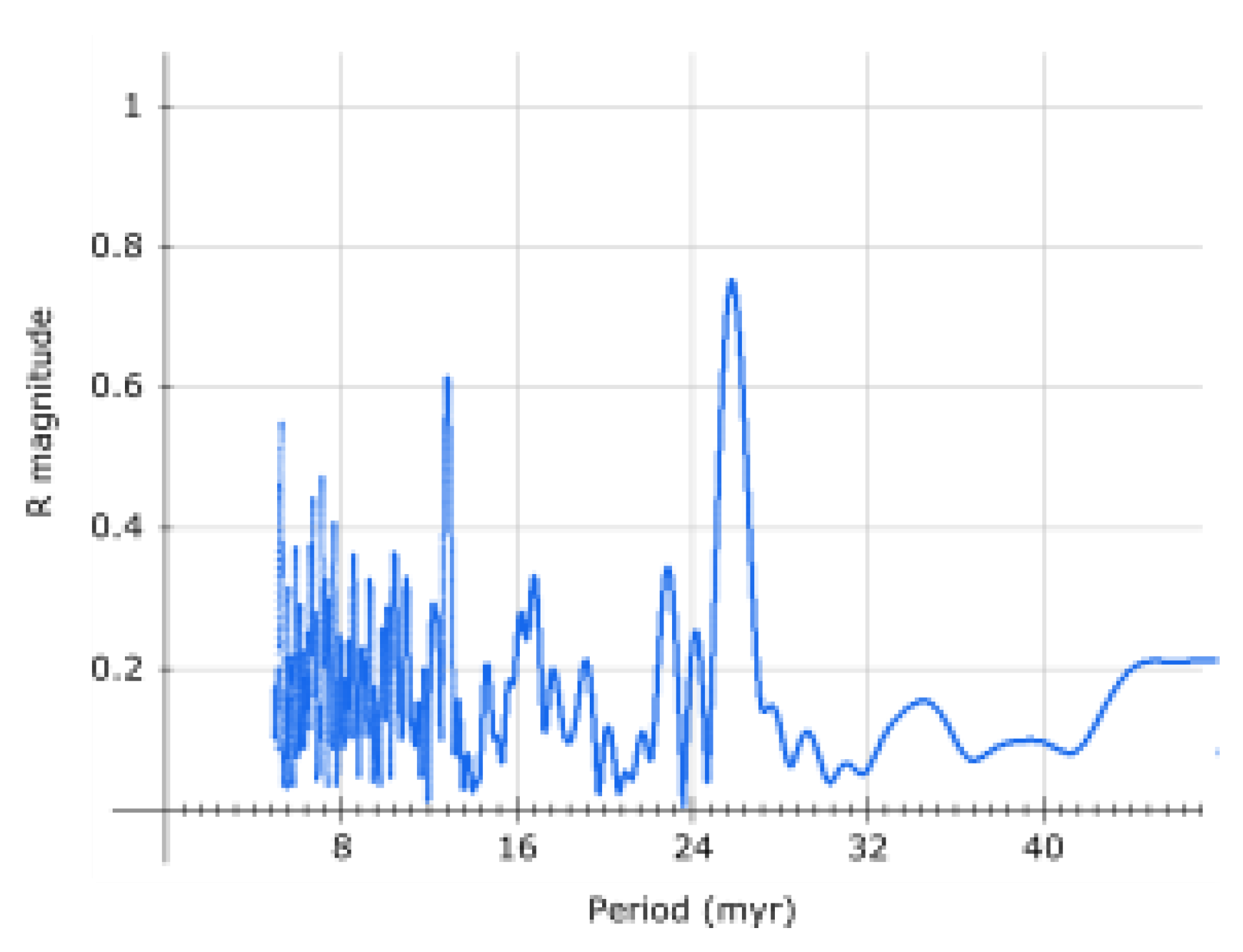
The R peaks at 0.75, corresponding to P = 25.84 My. Phase for this P is 9.78 My, however, here another peak at 12.875 My (R = 0.61) reveals a likely harmonic.
Dataset 6
Here, dataset contains only highest energy (major and minor) extinctions, from dataset 1. This dataset gives highest R maximum (0.837), a period P = 25.74 My, with a phase of 9.689 My.
Table 33.
Extinction events dataset 6.
| energy level | extinction events [mya] | extinction events (), age corrected [mya] |
|---|---|---|
| 5 | 66, 201.3, 252.2, 365, 445 | 61.986, 190.208, 238.316, 345.385, 421.148 |
| 4 | 37.8, 145, 260, 305, 420 | 36.206, 136.774, 245.993, 288.3, 397.519 |
Confidence
Note that equal weight was assumed for all extinctions in a particular dataset. Different weights can affect the confidence in the result (less if they are all harmonics). But even with that taken into account, there is high confidence in P ≈ 25.74 My - 25.92 My.
The result with the highest confidence (25.74 My) is also the closest to the calculated ideal quantization by the 3rd order period (1.512 × My) - 25.705 My.
Note that the burning cycle of the Sun’s core is calculated (in the chapter 19.3. Energy replenishment, burning cycles) to be equal to 25.7 My - 25.9 My, further confirming the signal.
Interestingly, taking into account major extinctions only, one of the obtained peaks (with R = 0.94) is at 25.705 My, exactly as needed for ideal quantization. However, as noted before, periodicity is unlikely to be perfect (absolutely it cannot be) and the period probably oscillates about some mean value. Interestingly, the values obtained can be correlated with Earth’s axial precession. The period of this precession was calculated by Newton to be 25920 years ( per 72 years), which is exactly 1000 times smaller than the value obtained with dataset 1 (25.92 My), suggesting that the axial precession period is a harmonic of the 2nd order period. However, the rate of precession varies with time and the current estimate for the period is 25771.71 years, closer to the value of 25740, which would be the result of division of 25.74 My (obtained with dataset 6) with 1000. Multiplication with 1006 yields 25.92634 My. If the period of axial precession is indeed a harmonic of the 2nd order period, then the two may vary in relative synchrony. If planetary orbitals/resonances are periodically reset (as hypothesized), then the axial precession period would be periodically reset as well. Interestingly, the value of 25.84 My, obtained with dataset 5, divided by 152 gives the current axial precession period for Mars (∼170000 years[272]). A more precise value for the Mars’ axial precession period (based on 7.576 arcsec/y[273]) multiplied with 152 yields 26.002112 My. The current axial precession period of Venus (derived from the predicted precession rate of 44.75 arcsec/y[273]) multiplied by 895 gives exactly 25.920000 My. This suggests that all axial precession periods of planets are harmonics of 2nd order cycles. But it does not end there. The period of perihelion precession of Mercury (5600 arcsec per century[274], or 56 arcsec/y) multiplied by 1120 gives exactly 25.920000 My as well. In any case, while the effects on Earth are not strongly periodic (e.g., extinctions are obviously not regularly separated precisely by ∼26 My), the 2nd order cycling might still be regular, suggesting that cataclysmic events on Earth are an indirect effect of this oscillation (e.g., gravitational disturbances of asteroids might be regular, but a disturbed asteroid might affect Earth immediately or after a few million years, or not at all, and the impact energy may vary).
Neurogenesis in standard lifeforms on Earth during embryonic development does imply certain, albeit flexible, periodicity or cycling in the formation of brain layers and neuron migration. High energy impact cratering and extinctions/migrations in planetary neurogenesis should be no exception.
With a fixed periodicity of ∼26 My and the last highly energetic extinction 37.8 My in the past, next one would be overdue, roughly by the phase shift.
Note that a delay of extinction could have some relative benefits due to more evolved progenitor neurons at time of differentiation, although with the cost of increased probability of cancer development.
Also note that neurogenesis implies correlation of many processes. Therefore, calculated periodicity should not be limited to mass extinctions, rather present in plethora of other phenomena affecting the planet - volcanism, magnetic reversals, seafloor spreading, orogenic events, etc.
Indeed, such periodicities have been found in previous analyses[275].
Should this be interpreted as flexibility in the process of neurogenesis or are there hidden variables?
As noted before, major extinctions seem to be grouped in pairs and multiple oscillators should probably be considered. With paired extinctions separated by roughly 63±3 My (in uncorrected ages), major extinction in the present time would be on schedule. This peak can be observed in analysis. Indeed, repeating the analysis for dataset 5, but with only major events (using corrected ages) included, yields highest peak at 12.85 My (the 2nd harmonic of 25.7 My) and R = 0.973, with the 2nd highest peak being at 59.272 My (R = 0.923).
Including current extinction (0 Mya) in the analysis gives highest peak at 59.74 My (R = 0.925) and a phase shift of 2.38 My. Note that, while the hypothesized 3rd order cycle period of 1.512 My is a harmonic of 25.7 My, the 2nd harmonic of 1.512 My (0.756 My) is a harmonic of 12.85 My and is then probably also a harmonic of the bigger period, in which case the correct period would be 59.72 My. Assuming synchronization with this harmonic (0.756 My), last major extinction 62. Mya (66. Mya uncorrected[276]) gives the interval for the current major extinction 48000 years before present to 6000 years after present. Interesting result, considering the extinction of megafauna (incl. Neanderthals) started some 50000 years ago. The age of 66.006 Mya (uncorrected) for the last major extinction would give exactly the present time for the current extinction.
In any case, this suggests the current major extinction is right on schedule.
Thus, imminent extinction (or the ongoing extinction peak) as calculated using models based on C1.1 equation should not be surprising.
Supplement
Here is the code used to calculate correct ages of extinction events, perform the analysis and generate images.(Fig.: getext.php +)
16.4.4. Correlation with Mantle Layers
Grouping and correlation of extinction events with the formation of brain [mantle] layers also indicates that another major mass extinction should be near, at least in geological terms.
This correlation is shown in Figure 28 - time between major extinction events of Phanerozoic is proportional to the thickness of the corresponding mantle layer.
Such correlation should not be surprising - all lifeforms grow in layers. But it also confirms the previous hypothesis that asteroid impacts are correlated with discontinuities (changes in energy levels) in Earth. Note that encapsulated growth/development is common in standard embryogenesis. It appears this is the case with planets such as Earth as well.
This is, effectively, a conversion of temporally separated discontinuities into events separated in space.
To quantify the correlation, periods of weak evolution and thicknesses of mantle layers have been normalized:
Results are shown in Table 34. Here, corrected extinction ages are used, although non-corrected ages would yield similar results. Correlation in absolute value varies between the pairs, but overall, it is apparent.
At least some deviation could be explained by the fact that formation is not yet complete - e.g., the boundary between layers 3 and 4 might change with the pending extinction.
If layer 3 decrease would be equal to layer 4 increase (≈ 0.0575 in normalized value) and layer 1 decrease to layer 2 increase (≈ 0.0275 ≈ 0.0575 / 2), with a small decrease in layer 5 (0.013 ≈ 0.0275 / 2) coupled with equivalent increase in layer 6, normalized extinction and mantle boundaries would be almost equal.
Effectively, what is necessary for better agreement is the upward movement of 3 discontinuities (between layers I and II, III and IV, V and VI).
There are two interpretations for the correlation. Extinction events are either memorized in Earth’s [brain] mantle as they occur or they are programmed events and can be predicted through the analysis of discontinuities (layers) in the mantle. The ongoing 6th major extinction and existing discontinuity at 100 km depth suggest the latter, although superposition may be more likely - discontinuities are ancient but they move/adjust as extinctions occur.
In any case, the correlation is good evidence for living Earth and its neurogenesis.
The entanglement of 3 discontinuities (I/II, III/IV, V/VI) suggests that all 3 move during a single extinction, thus, if movement is correlated with asteroid impacts, 3 impacts may be ahead.
However, exact location of boundaries is a matter of debate. They must have some thickness, so it may be more appropriate to equate layer thickness with distance between discontinuities. If that would be a distance between lower discontinuities of two boundaries, it would, for layer 1, yield a normalized value exactly equal to the corresponding normalized period of weak evolution:
Also, globally average velocities might not be the best choice for determination of layer discontinuities - e.g., Lehmann discontinuity is at 220 km for tectonic North America, but 200 km for shield North America [281], while it may be absent beneath north Atlantic and other oceans. Whether the discontinuity is global or not may depend on impactor energy and the stability of a graviton at particular energy level. If the discontinuity is not global, the impactor site should probably be antipodal to the discontinuity.
Note that layers in human neocortex also vary in thickness[282], depending on the area, so this is not unexpected.
No graviton can be completely neutral. At the time a discontinuity is occupied by a [large scale] graviton, a hole, proportional to polarization, is expected. Physical imprint may be further complicated with the presence of multiple gravitons and may be affected by additional disturbances.
If one assumes that 200 km is a proper boundary (220 km may simply represent additionally disturbed 200 km boundary, it may even be reduced again to 200 km with complete formation), the correlation with extinctions for both layers, I and II, becomes remarkable:
Some report the base of the upper mantle at 670 km[283] (it is also the average beneath China[279]) rather than 660, this improves the correlation with layers 5 and 4:
Now, the only problematic boundary is the one between layers 3 and 4 (at 520 km). Some do report this boundary at 500 km[284], which gives much better agreement:
Note that extinction boundaries also have some thickness or uncertainties, notably first three, which may explain differences in reported discontinuity depths. The 3rd major extinction (Permian) is apparently split into two events (End-Capitanian and Permian-Triassic). Using End-Capitanian 245.793 Mya (259.8 Mya uncorrected) instead of Permian-Triassic 238.041 Mya (251.9 Mya uncorrected) as the date of this extinction gives results in remarkable agreement with the obtained layers 3 and 4 (with discontinuities at 410 km, 500 km and 670 km):
The complete correlation, with above adjustments, is shown in Table 35 (with ages rounded to a single decimal). The correlation, using uncorrected ages for major mass extinctions, is shown in Table 36.
Interestingly, corrected ages are in all cases except for i=4 in better agreement with mantle layers. Unless an artefact of rounding/imprecision (e.g., in depths of discontinuities, which may be averages) this can be interpreted as evidence for effective time compression (pulses of abrupt temporary changes in decay rates of elements).
The excellent agreement here suggests no further adjustment of discontinuities is needed, except possibly for layer I, as shown in green in Figure 28 (right) which should be unsurprising given the correlation with the current extinction.
Correlation of layer 6 and the corresponding period of weak evolution has not been determined due to unknown boundary.
However, assuming the extinction at the start of Phanerozoic (511.664 mya in corrected age, or 541 mya non-corrected) is correlated with the lower boundary of layer 6, one can calculate the thickness of layer 6:
In that case, a discontinuity, if formed, should exist in Earth’s mantle at a depth of 937 km (assuming boundary between layer 5 and 6 at 780 km).
Apparently, this discontinuity has been detected[285] (at 940 km).
Using Most Recent Data
The precision in extinction ages has improved since the chapter was written. This is an update (2024.07.30), showing even better agreement with mantle layers.
Mass extinctions are not instantaneous events and, usually two years are associated with a particular extinction. In such cases, the average of the two is probably a better choice (especially considering that mantle discontinuities have certain thickness as well, and the average is usually used) and that average is used here. The Late Ordovician mass extinction is considered to have occurred ∼445-443 Ma[286], thus 444 Ma is used as the date. The Late Devonian extinction occurred about 372 Ma[287]. The Permian-Triassic and the Capitanian (also known as end-Guadalupian) extinctions are both extreme events and are very close together on the geological timeline. Thus, instead of using both, only the date for the Capitanian extinction was used. The Capitanian extinction occurred 262-259 Ma[288], thus, 260.5 Ma was used for the date. The end-Triassic extinction occurred 201.6 Ma[288], while the Cretaceous–Paleogene extinction occurred 66 Ma[288]. Results are shown in Table 37.
Note, however, that using 445.2 Ma here instead of 444 Ma gives better or equal results for all periods except for i=5, as follows: 0.164, 0.250, 0.132, 0.305, 0.148.
Table 38 shows the same using corrected ages. In any case, small deviation in correlation probably should be attributed to mantle instabilities, or oscillation/fluctuation of discontinuities over time. Discontinuities associated with graviton energy levels will probably drift from the level over time (e.g., due to changes in pressure/temperature), only to return and stabilize at the original position once the level is occupied again. Thus, higher deviation in correlation above may indicate levels that have been unoccupied for longer time. By the hypothesis, these should be the upper layers and that indeed seems to be the case. Small adjustment of the two uppermost layers (discontinuities at 200 and 100 km) gives perfect correlation for all periods/layers, as shown in Table 39. These discontinuities then should be adjusted with the upcoming impact(s). Note that energy required for a jump between energy levels is proportional to distance between the two levels. If these are adjacent levels, according to Table 39, energy required should be higher for levels at 500 km and 203 km. If higher energy here corresponds to higher impactor energy it probably also corresponds to a bigger extinction event. These two levels are associated with Capitanian/Permian-Triassic and Cretaceous-Paleogene extinctions, and these indeed are bigger extinctions than Late Devonian and end-Triassic. By that logic, assuming the current energy level is near 200 km and the upcoming is near 100 km, the current extinction strength should be between end-Triassic and Late Devonian in strength. However, if the current energy level is at 410 km (which may be more likely, if 410 km represents a stabilized state, while the uppermost two need adjustment), then the current extinction should be one of the strongest.
With the start of the Phanerozoic at 538.8±0.2 Ma[289] and the Late Ordovician boundary at 445.2±1.4 Ma[289], thickness of the layer 6 is:
A discontinuity then should exist at a depth of 780 + 140.7 = 920.7 km. Apparently, this discontinuity has been detected at 920 km[290], although it may not be global.
Some discontinuities show high global variation (e.g., the 670 km discontinuity ranges from 650 to 690 km). In case of discontinuities assumed to represent phase boundaries, the variation is assumed to be a consequence of temperature variation, according to the Clapeyron slope. However, the additional perturbation after initial boundary establishment can also be interpreted as mantle tissue gyrification, resulting in the increase in surface area of the layer (relatively equivalent to the gyrification of the brain mantle in mammals on Earth). As noted before, even if the conventional assumption is correct, multiple valid interpretations are common in nature.
The whole Phanerozoic seems to be linearly mapped to the mantle, but to what depth is this time-space correlation valid? Assuming it is valid all the way down to the centre of Earth, using Earth’s volumetric mean radius (6371 km), this would give for the age of the Earth:
where k (≈2/3) is the factor of time/space proportionality.
Although relatively close, this is lower than the conventional estimates of Earth’s age (not much lower, however, than the estimate with time compression taken into account). However, linear extrapolation may be valid down to the inner core. Inner/outer core discontinuity, assuming inner core size of 1216 km[291] would then correspond to 3.33 Ga (billion years ago). Interestingly, this is equal to the current estimate on the rise of Earth’s continents[292], and apart from mantle plumes, can be associated with a large impact 3.33 Ga[293]. The core/mantle discontinuity, assuming core size of 3486 km[294], corresponds to 1.83 Ga, which seems to be equal to one boundary of the "Boring Billion"[295], and could also be correlated with a large impact (Sudbury crater, dated to 1.85 Ga[296]). Extreme events at 3.33 Ga and 1.8 Ga have also been recorded on the Moon[297].
Interestingly, while the above calculated age does not represent Earth’s current age, that age can be obtained if one applies the temporal correlation to the lithosphere and atmosphere (up to the exosphere) as well. With atmosphere/exosphere discontinuity (thermopause) at 500 km[298], one obtains the age:
This is within the uncertainty of Earth’s estimated age of 4.54±0.05 Gy[299]. Considering that exosphere probably should not be considered as a part of atmosphere, or, as an intrinsic part of a planet (some smaller bodies in the Solar System, for example, have exospheres, but no dense atmosphere beneath), this may not be a coincidence either (although it is questionable whether the atmosphere itself should be considered intrinsic). Note, however, that the thermopause height varies, depending on energy input. Intense solar radiation can extend it far beyond the base of 500 km, up to 1000 km[300]. The value of k factor is also interesting, if fixed to 2/3, one obtains the age of 4.58 Gy.
Interestingly, using mesopause (discontinuity between mesosphere and thermosphere) as the boundary (≈85 km altitude), one obtains the age in agreement with previously calculated corrected age of Earth:
Using k fixed to 2/3, the agreement is even better, producing 4.3 Gy (calculated corrected age is 4.29±0.05 Gy). It thus appears that none of the discontinuities (whether internal or external) are random.
Resolving Potential Issues
While the high correlation is apparent in presented matches, there are potential arguments against the used values. Why using Capitanian instead of Permian-Triassic, or both? In other words, why is Capitanian correlated with a discontinuity, while Permian-Triassic is not? The reason behind this is simply the very small temporal period between the events, making it unlikely that both were synchronized with a large impactor, and since impacts are probably required for the correlation with discontinuities, it is assumed that only Capitanian was synchronized with a large asteroid impact event. One could then argue that a discontinuity at 520 km, rather than 500 km, should have been used in the comparison because it is present in more regions globally than the one chosen. In some regions, this discontinuity is present at 560 km, so the two (500 km and 560 km) discontinuities can be interpreted as "splitting" of the 520 km discontinuity[284]. However, that is just one interpretation. It is possible that for any large impactor an associated discontinuity should exist, and that major mass extinctions sufficiently far apart should be synchronized with such impactors. This does not rule out the existence of discontinuities uncorrelated with large impacts. One could ask why do grouped discontinuities exist? For example, why are there discontinuities at 500 and 560 km, instead of one global 520 km discontinuity? The reason for this may very well be impactors, in this case the Capitanian impactor, causing regional disruption of the 520 km discontinuity, or, perhaps global disruption of the 500 km discontinuity. Other discontinuity variations could be explained similarly. One could argue that, so far, only the Cretaceous–Paleogene has a confirmed impactor associated with the extinction. However, extensive volcanism - which is commonly interpreted as having a big role, could be associated with antipodal impacts[301]. For example, the subglacial topographic depression in Antarctica known as Wilkes land anomaly (assumed to be a 510 km wide impact crater[302], which would make it the largest impact crater found on Earth, although a promising candidate for a bigger one exists[303]) was directly antipodal to Siberian Traps (largest known volcanic event in the last 500 million years) ∼260 Ma[259], what is also the age of the Capitanian extinction. Siberian Traps are considered to be the primary cause for the Permian-Triassic extinction, largest mass extinction on Earth. It is possible that the impact responsible for the Wilkes land anomaly occurred at the time of Capitanian extinction (evidence for that age exists[259]), which resulted in the emergence of Siberian Traps. The period of time between Capitanian and Permian-Triassic of ∼8 My seems plausible for the emergence time considering the expected depth of melt associated with the seismically focused impact energy. Here, volcanism likely results from induced lithospheric cracking and focusing of asthenospheric melt, as magma is less dense then the overlying mantle and crust. In any case, if impactors are correlated with discontinuities (or, disturbance of discontinuities), this can be experimentally verified, as regions of disturbance should be correlated with the impact site. Note that this antipodal relationship between impacts and volcanism is not limited to Earth, it is also common on the Moon and Mars[259].
Obviously, correlation becomes less striking by choosing different values for discontinuities that vary in depth, but overall remains significant - variations are concentrated near the values giving high correlation.
Another potential issue is the inclusion of the 780 km discontinuity. All other values used can be correlated with well established global discontinuities, but this one represents a local reflector that may not have global presence (certainly not as a global discontinuity), and it is possible that many such local reflectors exist at various depths. However, this depth has been predicted once other matches for major extinctions were established. Why is this discontinuity not global and should it be? This may require further research, but if correlation requires impactors it is possible that during the Late Ordovician (∼444 Ma) there were no large impactors involved in the extinction, although potential large impactors do exist (Deniliquin[303], Ishim[304]). Another possibility is that impactor energy was low, as some correlation is likely to exist between impactor energy and the size of the discontinuity and/or the size of its disturbance (which does not imply, however, that discontinuities are formed at the time of impacts). Also, it cannot be ruled out that the 780 km reflector represents remains of once larger discontinuity. In that case, the impactor energy may have been high but discontinuity may have been relatively unstable (as noted, potential large impactors that can be associated with this discontinuity do exist). Late Ordovician didn’t lack impactors, however. In fact, a pulse of elevated bombardment seems to have occurred in Ordovician. Evidence exists that this was a consequence of formation and subsequent destabilization of rings of debris about Earth. It has been hypothesized that these rings have been formed through the breakup of a large impactor[77] (>10 km in diameter). Therefore, it seems that a large impactor was involved after all. Lack of the associated global discontinuity then could be correlated with its breakup and spreading of energy over space and time. Multiple ring-associated impacts have indeed occurred at or near the 444 Ma boundary[77]. Note that the 780 km reflector has been detected under Mudanjiang, Heilongjiang Province in China, which has been at, or very close to, the equator in Late Ordovician. Impacts at the time were also concentrated at the equator (correlated with rings), and many were found at the opposite side of the world, near the antipodal location to Mudanjiang[77]. This seems to suggest that the reflector at 780 km depth has moved with tectonic plates, however, other explanations are possible. In any case, this should be further investigated by studying other such correlations.
Why do correlations start at the 100 km discontinuity, not at Conrad, MOHO, surface, or some atmospheric discontinuity? Again, this can be explained by the proposed genetic coding, resulting in development qualitatively relatively similar to the development and growth of living organisms on Earth. For example, tree rings are highly correlated with changes in external conditions (seasons) and their duration, however, this correlation starts below the crust (bark). In a tree, the bark contains the oldest tissue, the youngest is below it. Still, based on fossil records, one could argue that what’s happening today is not even close to the destruction that occurred in the last 5 major mass extinctions. That is certainly true and it is possible that a 100 km discontinuity is inappropriate, however the current trends and rates of global changes strongly suggest we are on the path to a major global catastrophe. One could only question whether the tipping point has been reached or not, and if not, how likely it is that it won’t be reached? Furthermore, the lithosphere is a rigid layer of material and could be interpreted as the equivalent of a bone layer under the crust ectoderm (skin) enveloping the brain (or the equivalent of a bark layer in trees). Mantle below the lithosphere is not as rigid. Thus, in that sense, the chosen discontinuity seems appropriate. Similarities do not end there. Human neocortex has 6 layers and periods between 6 major extinctions here correlate to 6 layers in the Earth’s upper mantle (the Phanerozoic aeon may thus be interpreted as a neocortex aeon). Human skull is composed out of multiple plates that have been stitched together during development. This can be compared to the lithospheric plates, which will eventually become stitched and fixed as well (like it probably has happened on Mars). In any case, further research could verify some of the proposed explanations and the work could prove to be of scientific value even if the proposed hypotheses are rejected.
Possible Requirements
The case of correlation of Capitanian (∼260.5 Ma) and Permian-Triassic (∼252 Ma) extinctions with discontinuities suggests that larger asteroid impacts should be directly correlated with discontinuities, while major mass extinctions could be correlated indirectly. However, asteroid impacts may be associated with all major mass extinctions sufficiently far apart. Capitanian and Permian-Triassic are very close on the geological timeline and two large impactors within such short period are unlikely. The above analysis suggests that the impact should be associated with the Capitanian extinction, while the Permian-Triassic is a result of antipodal volcanism associated with the Capitanian impact. Large impactor and extensive volcanism[305] are both confirmed for the Cretaceous-Paleogene extinction (66 Ma). Evidence exists for the extensive volcanism in the Late Ordovician (∼444 Ma) extinction[306] and potential large impactors (Deniliquin[303], Ishim[304]). Evidence for extensive volcanism correlated with the Late Devonian (372 Ma) extinction exists as well. Interestingly, flood basalt events are estimated at ∼360 Ma[307], about 12 My later, which is consistent with the impactor at Late Devonian boundary considering expectable volcanism emergence time. Potential associated impactor[308], or even multiple impactors[309], exist. Massive volcanic eruptions are considered as the main cause for the End-Triassic (201.6 Ma) extinction[305]. Candidate impactors exist again, with the largest impactor (Manicouagan) reported some 12 My earlier, at ∼214 Ma[310], which, however was not antipodal to the End-Triassic volcanism at the time, rather occurred at the same site. However, antipodal relation is not required for the impact to be associated with melts and large igneous provinces occurring on surface 8-12 My later. Emergence at or near the site of impact should be possible as well[311], which may then be interpreted as a consequence of a reflection of the melt trigger. In case 214 Ma should then be used in the analysis (instead of 201.6 Ma), a discontinuity at 429 km instead of 410 km gives perfect correlation in Table 39, which is within the range of variation (∼405-440 km[312]). Interestingly, a peak at 430 km has been detected below the Korean Peninsula and southwestern Japan[313], it is also the depth of the discontinuity beneath northeastern China[314], but it is unclear whether this could be correlated with the Manicouagan impactor. Large igneous provinces (LIPs) may commonly occur 10±2 My after large impacts. Indeed, this seems to be the case for the Cretaceous-Paleogene (66 Ma) extinction as well, where LIPs associated with the birth of the Atlantic ocean (separation of Europe and America) occurred 10 My after the impactor, ∼56 Ma. These were some of the most powerful volcanic eruptions in Earth’s history. This was also the age of the Palaeocene–Eocene Thermal Maximum[315]. Unless there is no direct or antipodal relationship, or possible correlation in energy, LIPs may be hard to correlate with impacts, as they seem to occur relatively frequently. However, this frequency (every 20-30 My[316]) seems to be equal to the frequency of 2nd order impacts so the two probably are indeed correlated, the phase shift between the two can be explained as the time needed for magma to reach the surface. Although most energy is focused on the site of impact and its antipodal location, large impactors will create strong earthquakes globally and may increase effective permeability of the existing deep magmatic systems. In other words, they can trigger or significantly accelerate volcanism at various locations where magma chambers and mantle plume "heads" already exist. Thus, even strong volcanism that is not at the antipodal location of the impact site of a particular impactor may still be correlated with it, and here the emergence time is probably likely to be much lower (100,000 years or less). Indeed, this seems to be the case with the Cretaceous-Paleogene extinction, where the Chicxulub impactor provided a boost of energy responsible for at least 70% of the Deccan Traps[317] (the Wai subgroup).
A very interesting case is the discontinuity at ∼100 km. If we are amidst a major mass extinction, and if such extinctions are correlated with discontinuities (directly or indirectly), a discontinuity about 100 km should exist (with other correlations being correct). This discontinuity does exist, however, there were no recent large asteroid impacts, although a potential candidate exists (Bowers, ∼3 Ma[318], which, curiously, seems to have an antipodal hotspot - Jan Mayen island). This suggests the impacts (or at least flood basalts) are about to come in relatively near future.
Significance
All sub-surface (or, sub-lithospheric) major seismic discontinuities have been correlated here with major events on Earth’s surface, and this correlation seems to imply large impactors (asteroids and/or comets), although this may not be the sole requirement. Even if one considers alternative values for discontinuities exhibiting depth variation, significant correlation remains, even if not striking. And implied large impactors are rare. The Earth Impact Database lists only 6 confirmed impact craters with transient diameter ≥85 km[319]. Thus, the odds for this correlation to be a coincidence are low.
Effects on Angular Momenta
Redistribution of mass with energy level changes should have effect on [or be relatively synchronized with changes in] Earth’s angular momentum. Since, with time, mass is redistributed from the core outwards, slowdown of the Earth’s rotation should be accelerated during the redistribution, as well as recession of the Moon due to tidal coupling. With, overall, decreasing energy between transitions the effect should be decreasing as well. Indeed, studies confirm such evolution of Earth/Moon momenta[320]. Of course, if most mass redistribution has occurred in the earlier days of Earth’s formation (when the mass was hotter and less viscous), which probably is the case, effects during Phanerozoic transitions should be much less pronounced. However, even with no significant mass redistribution, since energy level changes involve graviton spin inversion and gravitational coupling/decoupling is neither absolute nor absolutely instantaneous, this spin inversion will temporarily disturb the Earth’s angular momentum. Since graviton [coupling] collapse is considered to be relatively rapid, the effect on Earth’s surface could be cataclysmic, as sudden change in rotation would result in inertial force driving strong winds and flooding of the land with water from oceans and lakes. Since the angular momentum is greatest at the equator, this is where the effect would be most pronounced.
Why is the Great Pyramid of Giza so massive and located at high elevation? It may have been built by someone who was anticipating such cataclysmic events.
Evidence for Earth’s Expansion or Something Else?
The results of the analysis above can be interpreted as evidence for the linear expansion of Earth since conception, however, any such significant expansion is unlikely[321]. Earth has been probably initially substantially compressed and then it quickly expanded to the radius roughly equivalent to the current radius. Due to cooling and decreasing rotation, the Earth’s radius should have been actually slowly decreasing since this early expansion. Some effective expansion is possible with the 2nd order impacts and associated graviton energy level changes, as these should be correlated with mass/heat/pressure redistribution. It is possible that hollow regions (similar to lava tubes) are created deeper in Earth with major mass extinctions (possibly correlated with the creation of habitable zones). If the material is expelled to surface and the stability of hollow regions is conserved over time (as noted before, this is possible with multiple gravitational maxima), the Earth’s volumetric mean radius could be increasing with the associated volcanism. However, the individual events do not have global coverage and the effect is obviously different from conventional expansion/inflation which can result in breaking up of continents. This is simply endogenous redistribution of mass, which, considering ages of rocks on the surface, obviously didn’t increase the radius much during the last 3 billion years. Surface expansion (stretching) can occur if some mass from hollowed out regions ends up stored somewhere below surface - causing land uplift, but even in that case the surface expansion is likely to be regional or small.
True global expansion of the radius of real mass is possible with the expansion of the large scale graviton beyond the Earth’s radius, however, the magnitude of the effect depends on the graviton energy density, energy density of real mass, and the strength of the coupling during transition.
Note also that the strength of local gravity should be decreased with graviton collapse (decoupling) - this too can cause expansion, although in the short-term (the collapse is temporary) the effect may be limited to gases (or fluids, in general). However, some fluids could be expelled to surface, atmosphere could expand as well, only to compress afterwards.
Recall that it has been suggested multiple times that Uranus is dead. The fact that it is larger than Neptune while at the same time less massive further suggests that the large scale graviton has indeed decoupled from its body permanently, thus, decreasing the local gravitational coupling (causing gas expansion).
Since it was hypothesized that asteroid impacts during major mass extinctions are the result of capture of nearby asteroids by large scale gravitons, it is indeed possible that some expansion of the Earth occurs with the end of an 2nd order cycle (implying that the asteroid is captured with Earth’s graviton expansion), but it should be followed quickly by contraction so there would be no net effect.
Note that some capture mechanism is probably required in order for these events to be locally coded genesis events. Since major mass extinctions and associated impacts have been correlated with discontinuities (energy levels) in Earth’s mantle, discontinuities in space also represent coded events in time (more precisely, the discontinuities represent coded soul-body transformation events). With relativity in causality, asteroids are only relative triggers of graviton energy level changes. Most likely, graviton collapse occurs prior to the impact, the impact is only synchronized with the settling of the graviton on the new energy level with the absorption of the kinetic energy of the asteroid. Collapse of the graviton here is a wave-like spherical expansion (delocalization) of the graviton, with finite range. Subsequent partial or full coupling of the wave with the asteroid, followed with localization back to Earth could sufficiently slow it down and put it on a collision course with Earth. Here, any artificial satellites are likely to be affected as well.
Graviton (wave) mass density at the Earth’s surface radius, should be, assuming the form of a 2-dimensional sphere:
m = graviton mass = 6.95 × kg
R = Earth’s radius = 6371 km
Assuming the wave is expanding at the speed of 2.93 × m/s, it has a significant energy density at the Earth’s radius. However, as long as the wave is expanding (tunnelling), with low coupling strength and fast transition virtually none of this energy should be locally absorbed (this is simply a transient disturbance of space, where matter in this space is only temporarily displaced).
Cumulative expansion of the radius in the last 4 billion years is probably not larger than about 66 km. This would be the equivalent of 6 hollow global layers of 11 km in average thickness each. However, such global layers may be unlikely (unless global discontinuities actually represent such layers). They are probably tubular, and, instead of being hollow, may be mostly filled with water.
Since major extinctions, major impacts and major volcanism are all correlated with discontinuities in the time-space correlation, it seems that discontinuities indeed could represent the hollowed out regions. In that context, it is interesting that the 100 km discontinuity represents the beginning of a low velocity zone that can be interpreted as globally present partial melting[280]. According to the hypothesis here where this discontinuity has been associated with the current extinction, this discontinuity should not be globally hollow at this point but it should be hollowed out sometime in near future. The heated up material at this depth goes in favour of the hypothesis and could then represent the material that will be expelled to surface.
In any case, the evidence from other studies does not go in favour of significant expansion of Earth. Thus, the results of the analysis should rather be interpreted as evidence of large scale genetic-like coding and planetary neurogenesis.
Correlation with the Human Cerebral Cortex/Neocortex
Qualitative similarity exists between the hypothesized Earth’s neocortex layers and neocortex layers in mammals. However, the best fit suggests that the layer I may not [yet?] be developed in Earth. Table 40 shows the comparison between the Earth’s mantle and the human brain, using normalized values, where values for Earth have been shifted by one layer up (better fit). The values here have been normalized without including the layer I, except for values in parentheses present in case of humans, which represent normalized values with layer I included.
Note that thickness of neocortex layers (even if normalized) can somewhat differ between different lobes of the neocortex. This could be correlated with depth variation in certain discontinuities within Earth. Deviation from the sample mean in the thickness of layers in humans used in Table 40 is ±10-m[322] , which translates to about ±3-10 km in case of Earth. Deviation between different lobes can be higher.
Since the upper layers of the neocortex appear to be exclusive to mammals[323], Earth’s neocortex profile seems to be mammalian-like. At this point, it looks more similar to the neocortex of primates than to that of the cetaceans (note that cetaceans have a thicker layer I, and lack layer IV[324]), and this is unlikely to change much with further development. Qualitatively, according to Table 40, Earth’s layers are very similar to human layers. The normalized thickness of the layer III with layer I included in normalization seems to be almost equal between the two, even quantitatively, and the relations between layers are roughly equal - e.g., in both cases, layer VI is significantly larger than layers II and IV, while the layer II is only slightly larger than the layer IV. Sorting layers by thickness then yields the same result in both cases: III, V, VI, II, IV, I. Is this correlation between Earth and the dominant species on its surface surprising? In the context of neurogenesis, probably not, if humanoid species have a crucial role in the functioning of the Earth’s neocortex. In any case, it seems humans are more entangled with Earth (and probably other bodies in the Solar System) than conventionally assumed.
Comparing thicknesses of layers II-VI through progressive brain evolution (mouse-rat-human) with that of Earth reveals interesting trends, as shown in Table 41.
Of course, humans did not evolve from rats or mice, rather from a common ancestor, however, it is probably safe to assume that a larger brain (neocortex) is a progressively more evolved brain (neocortex) in this case. Not all parts of the brain, however, evolve progressively - one layer of the neocortex may increase thickness at the expense of the other.
However, this is a comparison between different orders of life, and with a very limited dataset - inappropriate for derivation of strong conclusions. And what order should Earth belong to? Obviously, it cannot be classified into any order based on conventional understanding of life. However, in the context of CR, Earth can be a living being and, due to self-similarity of universes (scales), one could argue that it does belong to a relative large scale equivalent of the primate order, or the order of primate brains.
Comparing layers between different species within different orders in a larger dataset[325], some trends, potentially relevant here, can be extrapolated. Within primates, layer I tends to grow proportionally to the increase in the size of the neocortex, in both absolute and normalized values. Layers II and III combined tend to grow, from rodents to carnivores to primates, in absolute and normalized values. Layers IV and V show the inverse tendency, being smaller in primates, in normalized values. Layer VI also tends to be somewhat smaller. From this one can conclude that, with progressive evolution, or, evolution of intelligence, upper layers tend to enlarge at the expense of deeper layers.
This suggests that Earth’s neocortex is equivalent to a neocortex of a primate that is a bit more progressively evolved than human’s (cumulative normalized thickness of layers IV-VI is somewhat smaller in Earth, while the thickness of layers II-III is somewhat larger). In that case, it is possible that human neocortex is evolving towards an Earth-like neocortex (in neutral subspecies it may be more Earth-like already[326]). This neocortex symmetry may be a requirement for certain species to represent neurons or neural proteins associated with the intelligence of the host.
Based on trends within primates, Earth’s layer I should probably be ≥66 km, in which case the surface discontinuity could represent the upper boundary of that layer (its thickness being about 100 km in that case). However, this is probably unlikely - one reason being the exposure to space weather/impacts, some protective envelope should exist. Difference between human’s and Earth’s cumulative thickness of layers II-III and IV-VI is very small (it may even be attributed to standard deviation), suggesting that the difference in normalized thickness of the layer I should be minimal as well (note that the cumulative normalized thickness of layers I-III is roughly equal between a human, chimp and gorilla[325]). Thus, the thickness of the Earth’s layer I should probably be roughly equal to 66.75 km, or ∼67 km, which is then the lithospheric layer designated as layer B in Figure 28. The discontinuity that represents the upper boundary should then be at the average depth of 102 - 67 = 35 km. A very interesting result, as it is equal to the average depth of the Moho discontinuity.
Considering that the Moho is in some places beneath the oceans at a significantly shallower depth, layer I, or at least its upper boundary, may not be so inaccessible for an technologically advanced civilization. Vice versa is valid as well (surface may not be so inaccessible for life inhabiting layer I), and may explain some UFO/UAP phenomena (note that some of the UAP’s were observed diving into the ocean[327], and, allegedly, coming out of the ocean far away from the coast[328]). This raises a possibility that layer I is at least partially formed and habitable (at least for some species) already. The ongoing events as part of the hypothesized current neurogenesis event may even result in an increase in UAP encounters.
Note that the existence of this layer suggests that the current event may not be the final one, the final one would be the one correlated with the Moho discontinuity and should occur some 43 million years in the future. Additional 23 million years would correlate with the surface discontinuity. Interestingly, 43 My is the length of the Paleogene, while 23 My has passed since the end of the Paleogene. This suggests that the ∼100 km discontinuity should not be associated with the current extinction, rather with the Cretaceous–Paleogene extinction 66 Mya, in which case the current event correlates with the surface discontinuity and should probably be final. This interpretation further suggests that the layer I may have been completely formed 23 Mya. However, in this interpretation, correlation between other mass extinctions and mantle discontinuities is lost. Is there a solution that satisfies both interpretations? Yes. Note that the distance from the discontinuity at ∼100 km to the surface discontinuity is equal to the distance to the ∼200 km discontinuity. In other words, both distances cover periods of equal length (66 My). Now suppose that two large scale gravitons are involved in the oscillation between energy levels (discontinuities) correlated with transformational events (which include mass extinctions). One may associate one graviton with the first interpretation, the other with the second. A single temporal period may be correlated with two different spatial periods (layers) of equal length (thickness). In this case, the temporal period of the last 66 My is correlated with both, transition from the ∼200 km discontinuity to the ∼100 km discontinuity, and the transition from the ∼100 km discontinuity to the surface discontinuity. I believe this superposition is the proper interpretation. Does this imply that the current event is final after all? Not necessarily. It is possible that the final event will occur in the future, after additional 66 My. However, if there are 6 neocortex layers and the number of major mass extinctions should be equal to this number, another major event is unlikely.
Earth’s neocortex probably represents a superposition of 2 or 3 neocortices - male and female (correlated with the 2e state) of the same species and possibly an additional of a different species (see chapter 13.1.2. Standard model). In one interpretation, the superposition is not perfect (it cannot be absolutely perfect) and in one (e.g., female) the layering is shifted so its layer II is aligned with the layer I of the other. Thus, the total number of layers could be 7. This kind of superposition suggests that layers II-VI should be different than they are in the individual non-superposed neocortices, however, layers I and VII should be relatively unaffected. This then explains why the normalized thickness of Earth’s layer I is equal to the normalized thickness of layer I in humans, and predicts that the normalized thickness of layer VII should be equal to the normalized thickness of layer VI in humans. Indeed, in the original interpretation, the thickness of the layer VI (now interpreted as layer VII) was calculated to be 140.7 km. When normalized in proportion to other values in Table 40, the value is 0.208, very close to the normalized value of 0.201 of layer VI in humans. Note that the normalized thickness of layer I is the same between humans, chimpanzees and gorillas, but the layer VI is somewhat larger in chimps and gorillas[325]. Earth’s neocortex could thus represent a relative equivalent of the superposition of human and chimp (or gorilla) neocortices. Given the increasing equality between males and females and decreasing fertility in humans, humans could be indeed evolving to a some kind of superposition of male and female species. Given the growing aversion (correlated with decreasing fertility) between human males and human females, this male/female superposition might indeed be a superposition of different species. The interpretation of Earth’s neocortex profile that would give the best fit is probably not the superposition of equivalents of human and chimp/gorilla neocortices, rather a superposition of a chimp (or gorilla) neocortex and a neocortex that represents a superposition of human and canine (or feline) neocortices. Symbiotic relationship between humans and dogs/cats is probably a precursor to this convergence.
Alternative Neocortex Thickness
While it makes sense that the neocortex forms a dominating part of Earth, and although the major extinctions show good correlation with the proposed layering, it is possible that this correlation is not a correlation with neocortex layers, rather a correlation between layers of some bigger structure [of the brain]. Still, neocortex layering could be the same in relative proportions (due to conservation of self-similarity), it just may be smaller in absolute values, in which case the proportions may be similar to the proportions in mammalian brains. This gives, for a thickness of a human neocortex of 2622 µm[322], a total neocortex thickness in Earth:
= thickness of the neocortex in humans = 2622 µm
= radius of the human head = 57 / 2 cm
= Earth’s radius = 6371 km
The above calculation uses the ratio between a human neocortex and a human head. However, it may be more appropriate to use the ratio between a human neocrtex and a whole human body. In that case the Earth’s neocortex, for an global average human body mass of 62 kg[329], thickness becomes:
= human body mass = 62 kg
= density of human body mass (average between maximum inhalation and exhalation of air) =
An interesting value, equal to the previously estimated value for the thickness of layer I (using a density of human body mass of - which is the density with maximum inhalation of air[330], one obtains an even better agreement, 66.77 km). Again, likely location of this would be below the Moho.
Note that, if the Earth’s neocortex is analogous to the human neocortex, there should be no air in it, only oceans, there should be plenty of oxygen, however. Neural cells should not contain air either, rather a cytoplasm equivalent in the form of slightly alkaline freshwater with dissolved oxygen, delivered through magma channels. Life should exist in the salty oceans of the Earth’s neocortex, but also in neural cells. Intelligent beings associated with UFO/UAP phenomena may represent large scale proteins or microbes that usually live in these oceans and cells. The question is then how did they get to surface and is that normal for Earth-like lifeforms? Proteins/microbes living in human brains do actually have a way to get out. The cerebrospinal fluid (the small scale salty ocean equivalent), or CSF, can sometimes leak through the microscopic breaks in the barrier between the brain and the roof of the sinuses, and then drain out through the nasal cavity (I have experienced this myself multiple times). Similarly, it can also leak through the ears, but that is less likely. Obviously, the Earth doesn’t need and doesn’t have a nose or ears, certainly not in the form present in standard mammals, however, some cavities are likely to be present and barriers could be broken (note that these barriers are the thinnest beneath the ocean). Constant CSF leaks, however, are not normal, but barriers are likely to be absent during neurogenesis events. Thus, as noted before, the presence of these beings on Earth’s surface may indicate an ongoing neurogenesis event. This may not be limited to UFO/UAP phenomena, new species of fish or other oceanic lifeforms could be emerging from the depths.
Instead of asking ourselves, why are there no oceans (or life) on the surface of other terrestrial planets, we probably should be asking ourselves why is there [still] an ocean on Earth’s surface, instead of being somewhere in the deep? Indeed, as the ocean is a large scale equivalent of CSF, it may be sucked into the neocortex during the ongoing neurogenesis event. CSF on epidermis is only normal during embryogenesis.
Possible Evidence of Occupation of Core Energy Levels by Large Scale Gravitons
A recent study has found a low-velocity equatorial torus in the Earth’s outer core[331], near the core-mantle boundary (CMB), probably correlated with Earth’s geodynamo. Similar has been detected at the inner-outer core boundary. This could be interpreted as evidence for the [recent, current?] occupation of energy levels by large scale gravitons. The gravitons are hypothesized to have a torus shape, and if polarized, the torus should be more ring-like than spherical. The detected shape is thus exactly as predicted for a place where the magnetic field is generated. Is polarization of polarized gravitons intrinsic, or a result of the effect of induced angular momenta of nearby ionized matter? In any case, a rotational body should have different sources of a magnetic field. One field is directly associated with the graviton, the other is induced by Coriolis force. A decreasing strength of the Earth’s magnetic field, with no significant decrease in body rotation, may then indicate a change in graviton energy level and thus its spin momentum. If graviton is jumping to an energy level where matter will have a larger effect on its own angular momentum than vice versa, magnetic field strength may be significantly lowered. Note that the field associated with the graviton can, depending on its momentum, instead of strengthening, oppose the field generated by Coriolis force, which can be interpreted as magnetic field collapse.
Indeed, such state may be the case on Mars, which has a very similar rotation period to Earth. Therefore, the magnetic field of Mars could be relatively easily restored by the change of graviton energy level - enabling adult neurogenesis events on the surface.
16.4.5. Forms of Migration, Correlation with Religions
Although predicted as such, migration of life (at least one that represents proteins, not cells) from the surface to mantle layers does not necessarily imply transfer of living individuals (depending on transfer conditions, it may not even be possible to survive it). DNA may be all that’s required, but it is even possible that only souls (gravitons of smaller scale) are transferred - in which case, no physical tunnels are required, souls can simply tunnel through matter to a lower orbital radius, corresponding to a mantle layer. This interpretation does not require for Earth’s interior to have habitable zones, making it compatible with conventional models of Earth’s interior. Note that, assuming polarized souls represent polarized potential of Earth’s space, it makes sense for these souls to decrease the orbital radius with the decline of the magnetic field. This is an interesting interpretation in the context of Christian religion - if the heaven is up, the hell is down and, according to conventional models of Earth’s interior, it’s very hot down there, making it justifiable to claim that these souls will be burning in hell (even if not for eternity). A naked soul of the assumed scale should not be sensitive to the temperature of standard atoms, however, with no other living things, the soul is likely to couple with an atom [body] or an localized organization of atoms. It is still questionable whether a soul coupled to an atom can consciously feel the [changes in the] kinetic energy of the atom. It probably cannot - as atoms are extremely introverted beings, however, probability of dreaming hell could be proportional to the external temperature (as it has been shown that dreams can highly correlate with the state of external environment[332]). Old Egyptian religion is also interesting in this context. By that religion, souls of the deceased go to the Underworld, however, this Underworld is similar to the surface world and would be compatible with the hypothesis of habitable zones in the Earth’s mantle. In that interpretation, no physical tunnels are necessary, only deep habitability and existence of complex life (or possibility for its evolution/development) to which the souls could couple. Egyptians did not believe in hell (at least not as it is usually depicted in Christian religion), rather they believed that souls deserving to be punished are forbidden to incarnate into intellectual forms of life in the Underworld.
Whatever the truth is, I can already see even the most devoted Christians eventually converting to the Egyptian religion... Interestingly, the underworld is a common theme across different religions in the world, even when they have evolved separately. In is also interesting, that, according to the Old Testament, all human souls go to Sheol (a place of darkness, hell), regardless of the moral choices in life. This is consistent with the planetary neurogenesis assuming it is similar with standard embryonic neurogenesis - all neural cells go to populate the interior, the only difference is in timing and the layer of destination. Here, souls are discriminated, with more polarized souls occupying deeper layers (that is, at least, my interpretation based on the base correlation of soul polarization with electro-magnetism). This polarization can be correlated with morality - strongly polarized people are usually those who do the most damage to the planet and life on it. Thus, this soul distribution mechanism (and the correlated cataclysmic events) can also be correlated with the Judgement Day. Note that Earth’s magnetic field was stronger in the past. This goes in favour of the hypothesis as population of layers should proceed roughly from the bottom to the top. Interestingly, by the Greek mythology, the migration to the Underworld (Hades) on the Judgement Day includes a post-mortem spatial separation of souls. Also interesting are the predictions of the prophet Muhammad, among which is the prediction of accelerated time in the Judgement Day[333]:
"The Hour (Last Day) will not be established until (religious) knowledge will be taken away (by the death of religious learned men), earthquakes will be very frequent, time will pass quickly, afflictions will appear, murders will increase and money will overflow amongst you."
This can then be correlated with the hypothesized accelerated evolution and temporary increase in decay rates of elements.
Most striking correlation with ancient sources is, however, the correlation with old Vedic teachings, where the, here hypothesized, cycling periods of the 1st, 2nd and 3rd order can all be well correlated with the salient time periods in the Vedic cosmology[198]. The 1st order period is correlated with the Kalpa aeon. It is claimed that at the end of Kalpa the world is annihilated by fire. The annihilation at the end of a 1st order cycle is hypothesized here as well - most bodies of the system probably reduce to dust and asteroids. And this obviously involves high temperatures, as the evidence shows that rocks are altered/heated enough to recrystallize and reset the radiometric clocks.
However, migration to Antarctica probably is a migration of living individuals. Some may stay behind but these will probably migrate eventually even if not as living individuals (I have hypothesized elsewhere that every population of species contains polarized and non-polarized individuals and only one group of these is affected by strong evolution[334], similar is the effect regarding migration). This then can explain the unexpected negatively-skewed frequency distribution of body size for extinct dinosaur species[335] (although other explanations are possible). Further going in favour of the hypothesis is the fact that distribution was distinctly negatively-skewed only towards the end of major geological periods, when migration is supposed to occur. This suggests that the largest dinosaur species did not migrate, or that non-polarized individuals dominate in largest species - which I find more likely.
In case of the current strong evolution event, non-polarized individuals likely dominate in largest whales, while in humans non-polarized individuals still represent a minority. The fossil record past the current event is thus unlikely to contain humans.
But is human DNA destined for migration, or is it an uninvited guest? I assume if land animals are lured to Antarctica, then at least some of them should be neural progenitors, otherwise, all that matters is probably life in the ocean (which, however, can contain DNA of land animals, even if not in large amounts).
Considering high correlation of the hypothesized events of planetary neurogenesis with those of Judgement Day predictions of certain prophets, is there something else correlated with religion that could be useful to consider in this context? In Greek mythology, the "Erebus" usually refers to the Underworld, or the region through which souls pass to reach Hades (Underworld). Interesting then is the name of the volcano (and the volcano itself) that is active on Antarctica’s Ross Island - Mount Erebus, which sits on the Erebus hotspot. Could this hotspot be correlated with migration? Well, if it is indeed a hotspot (evidence exists for such interpretation) this implies deep roots, so it seems like a good candidate for the entry point. Studies are consistent with a plume of 250-300 km in diameter extending to about 200 km depth, when it narrows and extends further down to at least ∼400 km[336], possibly up[337] to 1000 km[338]. Such structuring is very interesting in this context. Apparently the plume narrows exactly when it reaches the hypothesized 2nd habitable discontinuity (correlated with the Cretaceous-Paleogene extinction). This suggests that, most migrating mass will be distributed over the two topmost discontinuities. Correlation with the Cretaceous-Paleogene extinction is even more remarkable considering that the Antarctic plate has apparently remained stationary since the late Cretaceous. This suggests that perhaps the same tunnel has been used for mass transfer in the previous major mass extinction.
Should one then interpret the naming of Erebus as coincidence, or a meaningful synchronicity event, correlated with subconscious influence on the decision?
Note, however, that the Mount Erebus is about 3800 m in height. This should not represent an insurmountable problem for the migration of humans into lava tubes (at least once the Erebus empties), but, as noted before, it does represent a problem for oceanic water (CSF), which is supposed to enter the tubes eventually. Thus, either the walls of the volcano will be melted, or this is not the entry point (at least not for the water), or there is no transfer of matter to the interior after all. It is possible that this is solely the exit point that may be further energized with an asteroid impact (possibly on the antipodal location). On the other hand, asteroid impact on the same location could destroy the walls of Erebus and depress the land, making the inbound transfer more feasible.
Interestingly, in Zoroastrian tradition, after the final battle of good and bad (which could be interpreted as Judgement Day) the figure known as Saoshyant ("the Saviour") would bring about a resurrection of the dead, after which the wicked will pass through a river of molten metal burning away all their sins[339]. The metal here comes from hills and mountains, melted by the spell casting Airyaman god and the Fire-god[340]. Should this be interpreted as the souls of the dead passing through the Erebus after the hills and mountains have been melted (including the walls of the volcano) by the asteroid ("spell") impact? Should the Fire-god be interpreted as the Sun - having a role in this? Interestingly, the Zoroastrian texts also explicitly speak of a mysterious demon who infests the sky during the "mixed state", falls on to the earth, and is finally burnt up in the flood of molten metal in which the human race has been purged. This would suggest that the asteroid ("demon") falls after the volcanism, however, the order of events in these texts sometimes depends on the source so it should be questionable. High relativity in causality ("mixed state" above could be interpreted as superposition correlated with this relativity) and multiple impacts during strong evolution are, however, possible, and even probable, as suggested by the planetary neurogenesis hypothesis. The texts also say that this demon will rush in through a hole [leading to Hell] that will be sealed afterwards by the molten metal. All in all, with the proper interpretation of gods and demons, heaven and hell, this sounds pretty much like the description of a planetary neurogenesis event.
More correlation can be found. In example, the Hebrew Book of Enoch (not included in the Bible), speaks of a patriarch Enoch who was taken on a journey with angels. The angels showed him a mountain with 4 recesses, 3 dark (housing evil souls) and 1 light (housing just souls) where the dead were waiting for judgement. The 3 dark recesses here could be interpreted as entrances to the 3 layers (discontinuities) of the mantle, while the light one could be interpreted as a tunnel leading back to surface. The book later says that the good will eat from the Tree of Life and regain the earthly body[339]. One could now interpret the angels as some beings who have a crucial role in a planetary neurogenesis event. They probably could be correlated with UFO/UAP phenomena, and, if so, these phenomena could be on the increase as we approach the "Judgement day". The Tree of Life probably should be interpreted as DNA. Now, in my theories, coupling of souls and bodies is highly correlated with DNA. To me, thus, this suggests that the "angels" will regrow the bodies of certain souls using DNA from the original bodies and the souls that were previously coupled to these bodies will now couple with the cloned bodies. Note that this can then be interpreted as resurrection. It is, in any case, the only scientifically plausible interpretation of Christian resurrection.
How to explain this high correlation of multiple religions with the hypothesis of planetary neurogenesis (and some other phenomena described here)? One interpretation is that the original prophets/shamans on whose teachings the religions are based could see the effective future/past in their visions and/or could expand their knowledge about the universe through these visions. In another interpretation, they were influenced (consciously or subconsciously) by some 3rd party possessing this knowledge. Both interpretations could be true.
In any case, I consider synchronicity (which I have, through my research and experience, found highly correlated with subconsciousness) to have a major role. Consider for example the Egyptian idea of the Underworld, which can be correlated with their ignorance regarding the Earth and the universe. The Egyptians associated the star Sirius (Sopdet) with the goddess Isis. They interpreted the rising of the Sirius above the horizon as the rising of the goddess from the duat (underworld). On her journey across the sky, the goddess was assumed to "die" in the western evening sky only to be "reborn" later in the eastern morning sky[341]. Not knowing the true nature of starts, the actual distances to stars and the size of the Earth, they’ve assumed that the goddess was, after "death" travelling underground in some form and that this underworld is habitable for that form. They, obviously, did not theorize planetary neurogenesis here, however, are the obvious correlations like this one meaningless coincidences, or should they rather be interpreted as meaningful synchronicity? I believe in the latter. All phenomena can be correlated with some kind of precursors. I interpret these ideas as precursors to the planetary neurogenesis theory. The Egyptian precursor even suggests that it is possible to escape from the underworld, at least for gods (which, again, may be correlated with UAP phenomena).
In any case, it is possible that, by studying the original teachings, one could learn more about the events. However, all these teachings have been, traditionally, corrupted over the years by polarized interests, making it hard to discern what could be trusted.
16.4.6. Evidence in Time Compression
If planetary neurogenesis is happening on Earth, it was likely happening on Mars and Venus too. Time, however, flows differently for animals of different size (which should be correlated with the scale of the coupled soul/graviton). The rate of evolution on Mars should then be different from the rate of evolution on Earth - it should be faster.
Applying Kleiber’s law, 4.54 billion years of evolution on Earth would, on Mars, last:
= Mars’ mass = 0.642 × kg
= Earth’s mass = 5.972 × kg
= 4.54±0.05 × years
Assuming Mars was formed roughly at the same time as Earth, present time on Earth corresponds to about 3.69 billion years ago on Mars (4.54 - 0.85 = 3.69).
This is a very interesting result as studies show that Martian climate shifted from habitable to uninhabitable - when its atmosphere was lost and liquid water disappeared from surface, roughly 3.6 billion years ago[342] (src[343]). In an even more recent study it was found that this liquid water was exposed to the atmosphere (rather than being covered with ice), up to 3.7 billion years ago - when the studied lakebeds dried[344].
This suggests that the current major extinction on Earth may indeed be the final major extinction of the planetary embryogenesis (neurogenesis), after which the Earth’s surface will become permanently uninhabitable (although periodic and possibly spatially limited pulses of habitability cannot be excluded, as hypothesized pulses of adult neurogenesis).
The same equation gives evolution period of 3.9 billion years for Venus, suggesting Venus lost habitability some 640 million years ago. Again interesting, as studies[345] show that Venus did lose habitability roughly 700 million years ago[346].
It is a common assumption that all planets in the Solar System have been formed at the same time (this is also the case with my theory of inflation of the system), and calculations above certainly can be interpreted as a confirmation of that assumption. However, the term is relative and a deviation on the order of millions or tens of millions of years is possible.
Early habitability of Mercury cannot be ruled out either. For Mercury, the equation gives a period of 517 My, with its end corresponding to about 4.0 billion years ago. Interestingly, this is also the estimated age of the most heavily cratered terrain on Mercury and the end of the Pre-Tolstojan period[347].
What about the Moon? The equation, for the Moon’s mass of 0.07346 × kg[348], gives a period of 167.7 My. Again, very interesting, as recent studies provide evidence[349] that the Moon formed about 4.51±0.01 Gya[350] and had a great resurfacing event about 4.35 Gya. This gives a period between the two of 160±10 My, in agreement with the calculated value. Using the obtained age for the mare basalt formation of 4336±32 Mya by Borg et al[351] instead of 4.35 Gya, the period of time between the two is 174±42 My. The average between these two is 167 My, roughly equal to the calculated value. Furthermore, assuming a period of time between the Earth’s and Moon’s formation is equal to the hypothesized 2nd order cycling period of the Solar System, with the 2nd order period equal to 25.92 My and Moon’s formation at 4.51±0.01 Gya, one obtains Earth’s age of 4.536±0.01 Gy, which is within the uncertainty of estimated Earth’s age.
The rate of evolution here should be proportional to both, biological and geological cycling. Thus, these should have proceeded at faster rates on early Mars. In example, the average rate of production of new crust during the Mars’ habitable period should have been about 5.33 times faster than on Earth. Magnetic reversals, on the other hand, are likely correlated with the Sun’s activity and Mars, being farther from the Sun, should be less sensitive to this activity. Magnetic dipole reversals on Mars during the crust formation should then be less frequent (proportionally to distance difference) than on Earth during the habitable period.
Assuming sensitivity inversely proportional to the square of distance (being dependent either on Sun’s gravity, electro-magnetic field strength, or, most likely, solar wind density[352]), with horizontal scale length of order 10 km on Earth for the width of features magnetized in normal, or reversed, polarity, the horizontal scale length on Mars should be:
= horizontal scale length on Earth = 10 km
= Mars’ distance from the Sun = 227.9 × m
= 149.6 × m
Thus, on Mars, magnetic crust anomalies should be 10 times wider than on Earth, and this is exactly what has been measured[353]. Given this and other evidence, plate tectonics had likely occurred on habitable Mars, only the number of plates, compared to Earth, may have been different. Recent studies also show that Venus must have had tectonics as well[354].
Interestingly, observations show stronger magnetism near the Mars’ south pole[355]. This could indicate that the magnetic field was confined to this area during the late stages of habitability on Mars (which should not be surprising if life is guided to the south pole, as hypothesized for the end of neurogenesis events). It could also be interpreted as younger re-magnetization (e.g., during an adult neurogenesis event). Both interpretations can be true. In fact, discrepancy between most recent measurements of Mars’ core radius (1650±20 km[356]) and previous estimates (1810 - 1860 km[357]) suggests a recent change in energy level of a major graviton, possibly causing core differentiation into a solid inner core and liquid outer core. This should then result in the creation of a magnetic field on surface (possibly also recreation of a stronger Martian moon) and may thus be interpreted as a signal of an upcoming adult neurogenesis event on Mars.
If lifecycles are faster on a smaller body, the sizes of organisms are likely to be smaller as well. If the size is roughly proportional to the host body mass, organisms inhabiting early Mars should have been about 10 times smaller than they are on Earth (although exact difference may depend on species and its environmental constraints). Indeed, potential evidence exists[358] for 10 times smaller microbes on Mars[359]. For complex lifeforms, however, other factors should be taken into account. Common limiting factor for the size of species on Earth is the spatial extent of the habitat. Island dwellers, for example, are usually much smaller than their mainland relatives[360]. Thus, considering surface area and assuming similar land/water ratio, compared to Earth, complex species on Mars should be about 3.5 times smaller on average.
It should be noted that the factor used in Kleiber’s law is to some extent dependent on the higher taxonomic ranks (e.g., order/class and up), with the factor 3/4 having the most significance in mammals. If this factor is valid for terrestrial planets, it could be correlated with the dominance of mammals on planetary surfaces during the last stage of neurogenesis. Note also that a significant difference in allometric scaling exists between organs, where the factor 3/4 could be interpreted as a superposition of factors for the brain (0.7) and the kidney (0.85), being closer to the brain. Dominance of the brain in planets should not be surprising, given their lack of motility and extroverted expression. In short, terrestrial planets are the brains or brain-like organisms. From the perspective of the Solar System, however, they could be interpreted as brain layers (where a single planet may represent multiple layers, depending on the number of coupled large scale gravitons). It may be something difficult for us to comprehend - due to vast difference in timescales, but the intelligence of these organisms probably should not be underestimated by anyone self-considered wise, as their genesis should obviously favour the neocortex development (at the expense of extroversion). This can be inferred from a different perspective as well - if their neural proteins are as complex as humans, how complex is their own intelligence? They might seem powerless and unreactive to human provocation, but this is just an illusion that’s probably very effectively dispersed during strong evolution events when their souls destabilize and intervals of time are compressed.
16.4.7. Some Additional Predictions of Neurogenesis
If the cultivation of complex life on planet’s surface is equivalent to the cultivation of neural cells during embryonic neurogenesis in mammals, the events hypothesized above are not the only upcoming events that can be predicted.
Obviously, cultivation of cells/proteins must be limited. The most effective (or most energy efficient) way to limit population growth is to substantially decrease its fertility. Recent studies show that fertility in humans is indeed decreasing, at an accelerating pace[361]. But possible ways to limit population growth are diverse and probably will be diverse. Fertility decrease does not have to be correlated exclusively with physical health (inability to produce offspring), it can rather be effective, e.g., through subconscious effects on human psyche or mentality. Generally, limitation of population growth can be correlated with:
- decrease in ability or will to produce offspring,
- increase in types of reproduction inhibiting sexuality (e.g., homosexuality, bestiality, etc.) and increase in asexuality,
- decrease of physical gender inequality or increase in physical attributes and behaviour decreasing sexual attraction between males and females,
- increase in male-female mental incompatibility,
- increase in socio-economic gender equality, reducing the need or will for partnerships,
- increase in acceptable sterile alternatives (artificial, virtual) or substitutes for sexual intercourse,
- increase in attraction and partnerships between younger (more fertile) and older (less fertile) male and female individuals,
- domesticated animals and artificial intelligence increasingly filling the voids usually occupied by children or partners,
- decrease in sexual compatibility (which can be strongly correlated with the above),
- increase in diseases that can be correlated with decreases in fertility (e.g., prostate cancer),
- decrease in nutrient-rich and nutrient-balanced food (health, development and fertility of species are all highly correlated with diet),
- increase in deaths (e.g., through wars, natural disasters, diseases, ...), assuming limit has been exceeded and population needs to be reduced to sustainable levels,
- etc.
Evidently, all of these are currently present, and most, if not all, are increasing in the society.
Of course, at least some of these effects can be attributed to humans (e.g., pollution may affect fertility directly), but even that should not be interpreted as absolutely non-coded or non-natural development.
Correlated with short-term interests, polarized or self-centric humanity obviously does not want to limit population growth (contrary, it promotes unlimited growth), however, something, correlated with long-term interests, is obviously acting against it. I don’t see much free will here, I see two forces, one seeking domination and the other its regulation. This may be common for the process of neurogenesis, where, in a healthy one, regulation prevails, and this then can be interpreted as domestication or taming of cancer, as regular part of embryogenesis.
Accelerated evolution also likely includes accelerated ageing in some species or sub-species (in some, possibly reversed), cases of which are showing up in studies too[362].
Our planet is obviously exhibiting self-regulation on many levels. This seems not to be limited to physical processes, but acts on mental ones as well - directly or indirectly. However, while regulation is a requirement for neurogenesis its presence does not imply neurogenesis. For example, it is probably not a coincidence that increasing pollution decreases fertility, which eventually decreases population, which in turn decreases pollution. This may have nothing to do with neurogenesis, rather simply survival of the planet. However, the presence of regulating [re]action on so many different levels may indicate something more complex.
16.4.8. Some Predictions Based on Past Major Mass Extinctions
If major mass extinction events are regular parts of neurogenesis events, they should be qualitatively, and even quantitatively in some aspects, very similar. Apart from the specific ocean pH value, another factor likely to be similar is the temperature, and/or changes in temperature. The global average temperature immediately prior to all 5 major extinctions indeed seems to have been similar, in most cases - if not all, about 22-C (although uncertainties exist and vary between cases). This was followed either by a drop or an increase of about C during the extinction, in all cases. In case of the Cretaceous-Paleogene extinction, there was also an temporary excursion in between that decreased temperatures by 5-C for months or even years (correlated with the asteroid impact). Since asteroid impacts have been probably involved in all major extinctions (although not as the primary cause), similar excursions have probably occurred in all of them, at least regionally.
Thus, a rise of about C of the global average, to about C, in the current event is probably in the pipeline. However, based on the analysis of past events, this could represent only a pre-extinction temperature (or a relative extinction-trigger temperature). Once that temperature is reached, either a drop or rise by additional C may be in the pipeline. What’s happening now may then be interpreted as priming for the extinction event. So when will C be reached? Extrapolating from current trends, about the year 2300. Again, however, this time interval could be compressed into the current century if the Earth joins the party.
Some might believe that humanity won’t allow for the temperature to rise by C, but serious psycho-analyses of this same humanity clearly show that that belief is fantasy. Humanity is not seriously trying to reduce emissions, the plan is to overshoot the, so called, "targets", and reduce the temperature later by sucking CO2 from the atmosphere by some large-scale efficient technology that is yet to be developed[363].
Since the analysis of past extinctions suggests that the temperature should drop or increase by C once C is reached, perhaps such technology may indeed be developed and will lower the temperature back to C. However, the analysis also suggests that this drop should be coupled with the extinction. So perhaps the technology will be in the form of a nuclear weapon, which, according to the current trends, would not be surprising either. In any case, I think I would prefer an asteroid impact over a nuclear war.
The data, however, may be misleading. It is possible that the current temperature (∼C), or the pre-industrial (∼C) one should be understood as the pre-extinction temperature. Uncertainties exist for global average extinction temperatures as well. A rise of C may not be necessary, perhaps a rise of C from pre-industrial temperatures would be enough, which could be reached by 2066, even according to conventional models (the RCP8.5 scenario) with natural feedbacks included.
A recent reconstruction of temperatures in the last 485 million years has revealed a consistent "apparent" climate sensitivity of ∼C[364], about two times larger than what is assumed to be today[365].
However, the estimates for the current sensitivity probably should be treated as minimal values, given the fact that, unlike past events, the current event is still in progress and much about coming natural feedbacks is not known with great certainty. Assuming that the current climate sensitivity then actually is C, doubling of the pre-industrial CO2 would correspond to about 560 ppm CO2, and the average global temperature of about C in the pipeline once that concentration is reached. Interestingly, with the effect of changes in albedo taken into account, 560 ppm effective CO2 has already been reached - in year 2024[365]. Thus, C of warming may already be in the pipeline, and the global average will indeed reach C, as hypothesized.
Interestingly, the 22-C is not only correlated with extinctions, the global average temperature in the last 485 million years ranges from ∼11 to C[364], giving the average of about C. Why do the temperatures in major extinctions go to the average? This temperature probably is the optimal temperature for the cultivation of life, or at least the complex lifeforms that represent Earth’s neural progenitor proteins or cells. This global average is probably also likely to be the regional average in places where these lifeforms will [migrate to and] live, for a couple of reasons:
- temperature differences between the poles and the equator are decreasing with increasing warming,
- as the event progresses, the energy for heating/cooling may not be available or easily obtainable, so if these lifeforms need to survive they will have to live in places where the temperature does not fluctuate much from the average (this is unlikely to be the case on surface - which probably won’t be habitable on average for other reasons as well, but it can be the case underground, e.g., in one-mouth caves the temperature tends to be constant and equal to the surface average (note that the number of caves should also increase with increasing volcanism).
Note that, with hypothesized strong compression of time with major events, a range of global temperatures of 15 - C, for example, that would, by the proxy analysis, seem to have occurred over a million years, would have been actually compressed to centuries or even decades, and evolution is probably most accelerated at 22-C. With this taken into account, differences in rates of climate change between past major events and this one effectively diminish, going in favour of the C climate sensitivity for the current event as well.
Apart from extreme temperature fluctuations, major mass extinctions involve extreme volcanism. Such volcanism is also highly correlated with a low magnetic dipole moment[366]. Thus, decreasing strength of the magnetic field should be relatively synchronized with increasing volcanism. However, even though the magnetic field strength is decreasing at the moment, it is still not lower than the long-term average. Due to higher relativity in causality and simultaneity on this scale (from our perspective), increase in volcanism can also precede the stronger decrease in the dipole moment. When considered alone, however, neither the decreasing dipole strength or the increasing volcanism can be interpreted as precursors of cataclysmic changes.
16.4.9. Adult [neuro]genesis
I have hypothesized previously that changes in energy levels of large scale gravitons are correlated with major mass extinctions and evolution of life in between. If different species of life are evolved between these major extinctions, the large scale graviton associated with these is not oscillating between adjacent levels, it is rather increasing or decreasing energy level with each major extinction. Here, progressive evolution may be associated with increasing energy levels, regressive evolution with decreasing energy levels. But what if the graviton is oscillating between two levels? In that case, relatively the same species should be evolved over and over again. This is exactly what happens in adult [neuro]genesis events. Once the highest energy level is reached, evolution (development) of new species stops. Occasionally, the graviton drops to a lower level before it returns back up, which should then be correlated with re-evolution of certain species.
Note that death events represent collapses of graviton/body couplings. In this collapse, graviton changes vertical energy levels, not horizontal, so, assuming direct transition, there is no regressive evolution of body components. However, the collapse may at least in some cases include transition between horizontal energy levels as well, which then should include evolutionary regression to some degree.
Note also that, assuming decay rates of standard unstable elements are temporarily increased with energy level increases, and temporarily decreased with energy level decreases, oscillation would imply no net effect on decay rates on larger timescales.
Adult [neuro]genesis events are probably generally spatially and temporally limited. Evidence exists for occasional limited pulses[367] of habitability[368] on Mars. Note that a relatively recent adult neurogenesis event on Mars also has the potential to explain some unexplained phenomena on Earth (e.g., some UFO/UAP sightings/interactions, greatest pyramids in Egypt). Some of the intelligent lifeforms re-evolved in the last Mars’ adult neurogenesis event may have, with the neurogenesis terminating extinction event, fled to Earth. Here they may have built the greatest pyramids (possibly even original Sphinx) as shelter, possibly using some kind of 3D printing machinery. They may have somewhat evolved since and probably still inhabit Earth (and/or Moon?), somewhere in the deep. As I have hypothesized elsewhere, modern Egyptian religion was probably formed once Egyptians encountered these structures. They associated them with gods, considered them sacred (this is one of the reasons why there are no original inscriptions in greatest pyramids) and started imitating them - to please the gods and to secure passage to the Underworld.
In fact, life matching or surpassing human intelligence may evolve prior to each major mass extinction (with temporary effective time compression solving flaws in the Silurian hypothesis), it just doesn’t last long on surface. It thrives somewhere, in some form, deeper underground (in some kind of underworld).
16.4.10. Problems, Solutions, and Alternatives
While partitioning of the Earth’s mantle, its correlation with major extinctions and cultivation/evolution of cells (life) on the surface do represent a strong signature of a large scale equivalent of neurogenesis, how plausible it is that migration of life to mantle does indeed happen?
It is possible that it does not - the Earth might simply represent a large scale of a [precursor] lifeform that is yet to evolve neurogenesis.
The Earth may be a large scale proto-organism which is at this stage not much more than a catalyst providing favourable conditions for the evolution of a coherent large scale lifeform. Sea walnuts (Mnemiopsis leidyi), for example, could, in that context, represent future cells of a large scale multicellular organism, or some multicellular part of that organism. Observed common fusion of individual sea walnuts[369] can be interpreted as a precursor event signalling that evolution is heading in such direction. However, such interpretation is biased towards our experience of multicellular life. Multicellularity on large scale may be similar to the multicellularity on our scale, but to what degree? Should one expect for cells to be physically glued close together in a large scale multicellular interpretation of life? Multicellular entanglement and intercellular communication on this scale may be less dependable on distance. After all, as shown previously, inner and outer planets can be entangled in stable states across large distances in space/time (although with scaled metric, these distances may not be as large). Now, cells like Mnemiopsis leidyi are much smaller than planets but they are also much larger than standard cells forming our bodies. Thus, requirements for multicellularity of life could be significantly relaxed relative to the scale of cells forming our bodies.
Perhaps life evolving on the surface will, on its own, eventually start digging deeper and deeper into the Earth’s mantle (as surface habitability decreases) - in the process changing the environment and making it more suitable for complex life (the process may be somewhat similar to how the standard cell acquired bacteria which evolved into mitochondria).
Note however that this as well could represent the coded migration event of the neurogenesis.
Thus, even if the Earth’s mantle doesn’t have habitable regions at the moment, it’s probably evolving in that direction.
But why then would mantle discontinuities correlate with major extinctions? This could be interpreted as a precursor of formation of habitable layers, but is it possible that the habitable regions have been created already?
To answer that question one first needs to determine what are the requirements for complex life to survive in the mantle. These appear to be: water, energy and suitable pressure (temperature) and density. The availability of water and energy probably should not be questionable (these are already predicted/confirmed with conventional theories/interpretations). The only issue then is the suitable pressure and density, enabling liquid water among other things.
I assume the layers are created and sustained with oscillation of a large scale graviton (if not permanent presence of multiple gravitons at different energy levels). Presence of a graviton will result in concentration of matter (real mass) about that maximum. Once the graviton changes energy level (through spin reversals and temporary scale collapse) the accumulated matter will remain stable for some time (millions of years or more) but periodic presence of a graviton can ensure long-term stability. This mechanism (oscillation between energy levels) can thus create alternating gradients of gravity where gravity is cancelled at some point between two energy levels, enabling thus the establishment of pressures/temperatures suitable for complex life.
Is it possible that such places exist in Earth’s mantle?
It certainly is - even without involving large scale gravitons, density can have multiple maxima, but there are constraints on size and shape (a habitable layer may be represented by a relatively hollow tube in the shape of a torus, or it could be quantized into multiple spherical cells).
Interior of the Earth has not been observed directly to significant depth so one must rely on indirect observations. The mass (average density) of Earth has been determined from laws of gravity and planetary motion, and is known to very good precision. Moment of inertia of Earth has revealed strong concentration of mass about the centre. Earth’s core thus must be, on average, more dense than the mantle.
Astronomy (tidal interactions) also revealed that Earth’s mantle must be, on average, rigid (solid).
Everything else known about the interior (including core size) comes from seismology, which is limited and very prone to interpretation bias.
Interpretation is possible once the paths and velocities of seismic waves are determined. The velocity is generally proportional to pressure (through coefficient of stiffness and shear modulus, which also depends on temperature) and inversely proportional to density. To determine pressure one needs to know the density. Obviously, the same velocity can theoretically produce infinite combinations of pressure and density.
Constraints can come from wave dispersion analysis (for shallow depths) and from modes of free oscillation[370] (which is especially valuable, as it can give averaged density in absolute value - independent of elasticity).
The conventional interpretation of the interior is usually based on 1-dimensional (density dependent solely on radius) models (e.g., PREM), where density in the mantle generally gradually increases with depth. Pressure may then be determined from calculated density.
Although 3D models exist as well, due to limited resolution[371] (averaged values) - which decreases with depth, density can oscillate/deviate from the prediction (model) and some areas in the mantle, especially at depths with high lateral heterogeneity, could have much different pressure and density (and composition) than assumed. Due to poor resolution of free oscillation and absence of earthquakes (ray-paths) throughout most of the mantle, and multiplicity of assumptions in interpretation, existence of low-pressure habitable zones cannot be ruled out.
It is also possible that habitable zones are hidden from view - e.g., in regions (e.g., tubes, spheres) of effectively curved space where sound waves simply wrap about the region. Here, this is not necessarily a localized spacetime curvature (which, by conventional theories, is not even possible here) rather a material acting like an acoustic invisibility cloak (such materials are definitely possible and have been created by humans already). After all, it makes sense to hide intelligence (or habitable zones) from outer threats (e.g., cancerous homo, earthquakes).
However, the non-existence of such cloaks does not rule out habitable zones in the mantle. Sharp transitions, strong S-wave reflections and S-P/P-S wave conversions could indicate a presence of low pressure fluid-filled zones (gas/liquid) and such reflections/conversions have been detected at mantle discontinuities[372].
In any case, surface tension at boundaries must be smaller than the compressive strength of the material in order to ensure stability. This can be solved elegantly with the existence of large scale gravitons and multiple gravitational maxima. But it is possible, at least for smaller objects, even in the framework of established theories, through small black holes[373]. Note that, similarly to a conventional black hole, mass of a large scale graviton is concentrated, usually over a thin spherical or a ring-like region (in fact, a black hole can be explained as a special case of a large scale graviton). For the calculated graviton mass, mass density of the graviton of Earth’s upper mantle radius would be about 33 times higher than the assumed average density of real mass.
16.4.10.1. Mechanisms of Creation
Materials requiring high-pressure for formation are sometimes expelled to Earth’s surface during volcanism. While high-pressure zones probably do still exist inside Earth, the existence of such materials does not imply current or global high-pressure conditions. Some materials may have been created during high-pressure conditions at the time of Earth’s formation. Indeed, the hypothesis on soul-body coupling on this scale implies initial condensation of matter, with subsequent mass redistribution correlated with graviton energy level changes. Changes in energy levels are likely synchronized with collisions of the planet with other bodies, which affect angular momenta and increase heat, stimulating expansion of matter. The excited graviton then does not have to have high energy in order for disturbed matter to concentrate about the graviton radius. In other words, graviton itself may not be redistributing matter, rather guiding it to concentrate at particular location, enabling low-pressure zones between energy levels. I also find it likely that collision energy decreases with time. The first collision (with Theia) was most energetic, temporarily expanding graviton radius probably beyond the current surface radius. The graviton(s) subsequently receded roughly to the current surface radius and this loss of energy should probably be correlated with the creation of the Moon. Next, the lithosphere was created, as the graviton(s) receded to the ground level. Subsequent impacts were asteroid impacts resulting in the creation of layers between the inner core and the lithosphere, starting from the bottom towards the top. These may have also resulted in the creation of moons (progressively smaller over time) but some or all of these may have not escaped Earth (if some did they may have been absorbed by Luna). The uppermost layers of the mantle have been created, or at least adjusted, during Phanerozoic and, as shown, can be correlated with major mass extinctions on the surface. This implies that each of these extinctions included asteroid impacts, albeit of progressively smaller energy. And this is why one can probably expect asteroid impacts during the current extinction as well.
Note that this kind of development is equivalent to embryonic development of animals on Earth, where the creation of ectoderm (outermost layer) precedes the creation of inner tissue.
Note also that the moon creation hypothesis explains antipodal anomalies. If asteroid impacts are relatively synchronized with creation of energetic moons inside Earth, ejected in the opposite direction, starting from the layer correlated with current graviton energy level, this can result in antipodal anomalies such as volcanism (e.g., Siberian Traps).
Impact should be relatively synchronized with the jump in energy level, but such excitations are unstable, resulting in immediate de-excitation and ejection of mass towards the antipodal location. Whether the mass will actually be ejected away from a planet will depend on the impact (excitation) energy and energy and state of the planet. In the early days of Earth’s formation the mantle was liquid and the energy of impactors was higher, so the probability for the ejecta to escape Earth’s gravity and form a satellite was also higher. Note that such mechanism of Moon creation explains high similarities between the mantles of Earth and the Moon (in conventional scenarios, the Moon’s mantle should be enriched in impactor material and should therefore differ significantly from Earth’s mantle, but that’s not the case[374]).
As the planet ages and cools down, outer materials harden and the crust is formed while impactor energies decrease. Thus, ejection of material becomes unlikely, however, induction of significant antipodal volcanism is still possible.
If the hypothesis is correct, this should not be limited to Earth. Indeed, the Tharsis region (bulge), especially Noctis Labyrinthus/Syria Planum area, on Mars, looks exactly like being produced by a spherical body hitting the lithosphere from below. The effects of this on surface should include terrain elevation, crust fracturing and volcanism. The resulting effect on the crust below the surface would be similar to magmatic underplating (thickening of the crust), which may have been detected as well[375]. Interestingly, there is a large impact crater (Isidis Planitia) antipodal to the Syria Planum. Note that plate tectonics on Mars has stopped, probably a few billions of years ago, enabling for antipodal correlation to remain conserved over such long time.
Note also that direct antipodal correlation requires direct asteroid collision with the planet (), and such asteroids may be the only ones carrying enough energy for energy level changes.
While the initial energies were higher and there was enough energy to eject material far away, the energies involved decrease with time and eventually there won’t be enough energy to breach the surface layer. In case of the former, satellites in stable orbits can be formed, in case of the latter, only a mark in the form of fractured crust may remain. But what about intermediate energies? In that case the body would be ejected from the planet, only to fall back down and get absorbed again. As the body is ejected, a lava pond (or, water pond - in case of icy worlds) would be left behind. Then, as it falls back down and sinks, it would create ripples in that pond. As the lava solidifies, concentric rings would be left imprinted in the terrain. Indeed, such imprints have been observed on celestial bodies (e.g., Callisto and Europa[376]), most recently on Venus[377]. Note that a conventional explanation for these structures requires two impactors hitting the same place over a very short period of time. How likely is that? Such scenario would be possible in the early days of formation. However, during that time the planet is much hotter and the entire surface may be liquid (this is almost certain if there’s a high probability for two asteroids to hit the same place twice during a short period of time). Considering the fact that fossilization of ripples requires relatively fast cooling, such events cannot occur very early on, rather at some intermediate period, consistent with the hypothesis presented here.
Interestingly, the size of the imprint (Haasttse-baad Tessera Ring Complex) on Venus (∼1500 km) is very similar in size to the anomaly below the Mars’ Tharsis region[378].
Depending on energy and the place of impact, asteroids alone may not be a threat for life globally, however, coupled with antipodal volcanism the threat increases significantly. It is also questionable, at least for the initial collision (with Theia), whether the two colliding bodies were fully formed prior to collision. It may be more likely that the event involved coupling of relatively naked gravitons where standard mass was acquired during the coupling (in which case, the event probably should not be interpreted as collision). The initial form then should have resembled a doughnut, with well mixed mass. Collapse of one graviton to a lower energy level would create the, more dense, core, and would be relatively synchronized with differentiation. Another collapse would then be synchronized with the ejection of mass in composition equal to the Earth’s forming mantle. This mass, of course, would then form the Moon. This scenario is, indeed, supported by the exploration of the Moon and most recent studies[374].
Note that, depending on the angular momentum prior to collapse, the ejection may not be the appropriate term in this case. What if the initial graviton radius was much larger than the current Earth’s radius? Suppose it was beyond the current Roche limit, and the graviton is a superposition of two large scale gravitons of significantly different energy. A collapse of a graviton with higher energy would cause most of the standard mass to collapse as well, however, the smaller graviton quantum may not collapse exactly at the same time. Its collapse beyond the Roche limit and synchronized concentration of leftover standard matter would result in a satellite (forming the Moon), which now may be interpreted as external localization.
Note that, in case of standard atoms, an excited electron can similarly be interpreted as superposition of graviton quanta (electron + photon).
Note that, due to relativity of causality, it is possible for a precursor volcanism to occur before the antipodal impact (in fact, the existence of precursors in general could be interpreted as one consequence of relative causality). A precursor impact cannot be ruled out as well. This may allow for certain predictability of the major event. However, since a precursor is inevitably shifted in time, its spatial coordinates may differ from the main event position as well (probably proportionally).
16.5. Metabolism of a Homo-Dominated Organ(ism)
Transfer of energy in wild flora and fauna is normally balanced both horizontally and vertically. Vertical transfer of energy is a part of the metabolism but changes in horizontal currents affect the vertical transfer too (and vice versa).
Humans, however, with their large effect on both horizontal (surface based) and vertical (Sun - Earth interior) energy distribution and transformation, are currently the major drivers of change. Horizontal dominance here is established with the increasing number of humans and domesticated species at the expense of decreasing number and diversity of other species, vertically, it is the dominance in the exploitation of the absorbed and accumulated energy of the Sun in the Earth’s ecosystem.
Thus, one may interpret humans either as metabolism energy carrier particles or consumers of that energy as cells of some precursor organ of Earth.
With a human population N of 7.674 × , average mass m of 62 kg[329], and average lifetime Δt of 72.6 years (data for year 2019, except mass - 2012), human power and associated basal metabolic rate:
where M is the mass of the Earth (5.9723 × 1024 kg).
This gives a value of 0.756 for the exponent, in agreement with Kleiber’s law. However, in case of a mammalian-like organ interpretation, the exponent suggests a superposition of a brain and a kidney[379].
Note that Earth has kidney [precursor] equivalents on surface[380].
In order for this superposition to differentiate into the brain, the exponent would have to reduce to 0.7.
There are several ways to achieve that (sorted roughly by probability, from highest to lowest):
- increasing human lifetime (≈25 times) to 1813 years,
- reducing population (≈25 times) to 307243423,
- reducing mass (≈25 times),
- increasing Earth’s mass ≈100 times (≈ mass of Saturn).
If humans are indeed progenitor proteins of neuron proteins of Earth, as carriers of energy of its brain metabolism, I would expect the solution to be a weighted superposition of the above.
Note, however, that the above does not take into account the human food intake. Taking that into account (1.5 kg/day = 39776 kg/lifetime) one obtains a value of equal to 0.87 (exactly equal to the value of the exponent for mammalian liver[379]). Considering that the value of the exponent depends on population size, this high agreement suggests that population may be at or near its peak. Is it surprising for Earth or its organs to be mammalian-like? Probably not, as it is clearly dominated by mammals (causality here goes both ways - one could argue that Earth is dominated by mammals because it itself is a relative mammal).
Note that the contribution of human rest mass is much lower than the human food intake. Disregarding human rest mass, thus, produces a very similar result (0.87). Do humans then represent cells that are about to form the Earth’s liver?
Note also that the liver is exclusive to vertebrates. One could thus argue that Earth is also (at least currently) a vertebrate-like animal.
If not, calculating with food intake, the number 25 above should be replaced by the number 15976 to match the exponent required for brain cells. Note that multiplying human lifetime with that number produces a number on the order of magnitude of a million, the same order of magnitude as the 3rd order Solar System cycle period (Earth’s lifecycle or lifetime period). Assuming that the lifetime of Earth’s neuron cell should be equal to the Earth’s lifetime period (1.512 My) - a reasonable assumption, the population should be increased to 10.004 billion to match the exponent of 0.7. Interestingly, according to UN projections[381], the population should peak at about 10.4 billion, and this peak is expected to be reached in the year 2084 (when the number of deaths should exceed the number of births) - which is exactly equal to the, earlier calculated, year of the end of Holocene. According to the same source, 10.004 billion will be reached about 2060.
Humans, at this point most likely should be associated with progenitor liver cells but have the potential to become associated with Earth’s brain cells. This, however, probably requires for human lifetime to be significantly increased (note that neuron cells are the longest-lived cells in mammals, most lasting the whole lifetime of the individual). If this will be achieved, it will probably be achieved with the proportional decrease in the rate of ageing. It does make sense that the rate of ageing of neurons is synchronized with the rate of ageing of the host.
It is very interesting that the physical form humans are evolving into is very similar to the form of grey aliens (at least according to my hypothesis[201]), putative extra-terrestrial beings that are visiting Earth. Assuming these beings represent brain cells of some planet (Mars?) and their rate of ageing is as slow as hypothesized, the metabolism related to extroverted expression (e.g., physical movement) is, most likely, significantly slowed down as well (our neurons, for example, do not move at all). It would then be extremely hard for us to communicate with such beings - on the extreme end, it would take them about 6 hours to communicate what we can communicate in 1 second. This probably rules out conscious communication, but possibly not meaningful one-directional subconscious communication. They may have evolved some kind of telepathy - which makes evolutionary sense, as they would be too slow to react on any kind of physical threat by physical force. It seems very reasonable to expect for such beings to avoid still evolving humans, especially if the environment is unsuitable for subconscious communication. Suppose that an adult neurogenesis event occurred on Mars some 1.5 million years ago and some of the developed cells did not migrate into the Martian interior for some reason (possibly by accident, but it is also possible that certain subspecies do not migrate by default). At least some of these individuals would have probably migrated to Earth, and, with such long lifespan, at least some could still be alive today. And if that’s true, these "people" are certainly more likely candidates for the original builders of peculiar great structures that can be found on Earth (such as the Great Pyramid in Giza) rather than our own ancestors whose technology was either non-existent or severely limited at the time.
I, strive for neutrality - the equal, balanced usage of all parts of my universe. I am aware though, that this is an unreachable singularity, but it is the journey that makes one alive - for without it there would be no senses, for a sense of reason, and a reason for existence.
16.5.1. Potential Issues
The lifetime of an Earth’s neuron cell and the associated proteins involved in the metabolism is probably 1.512 × years. If the ageing of humans is slowed down sufficiently to reach this lifespan, the food intake per day should decrease significantly but the food intake per lifetime should remain the same - if the change in the rate of ageing applies to all organs and tissues equally. But should the increase in lifespan be fully attributed to the slowdown of ageing? Perhaps the slowdown is only a part of the solution leading to lifespan increase. Suppose that the difference in ageing is equal to (ratio of the speed of light between the standard scale and U1 scale), instead of 1.512 × /72.6. With ageing decreased only by that ratio (102.3 times), with lifetime remaining the same (1.512 × years), lifetime food intake must increase 102.3 times. Thus, in order to reach the exponent above, the population must reduce by the same number, requiring 97.77 million individuals, instead of 10.004 billion. Energy is, however, correlated with . Assuming then the proper ratio is ()2, one obtains about 1 million individuals. So what is the realistic outcome/ratio? Arguments exist for both, the higher value and the smaller values. Consider, for example, the migration to Antarctica. Even if it becomes habitable, can it support 10 billion people? Unlikely. Ten billion people could fit in lava tubes if they are sufficiently long and large, but migration to lava tubes should probably involve a precursor settlement on the surface, in which case even 100 million seems too much to be sustainable. It seems that, either the migration will not involve living individuals (in which case most or all of the population will die in the extinction), or the migrating population will be limited (in which case, most of the population will die in the extinction). But there are other possibilities. Perhaps, for example, the settlement on the surface will be a settlement with a relatively fixed number of individuals at any time (a training base, or a transit station[382]) but a temporary habitat for most, where incoming people would only spend some time before they proceed into the tubes.
On the other hand, entrance(s) to the tubes (leaks or not) may already exist at the bottom of the ocean and, assuming some stories of alien abductions are true, some humans may have already migrated (as DNA, or clones) without knowing it. Natural selection, perhaps?
16.5.2. Additional Discussion on the Relative Nature of Homo
Dominance of lifeforms changes over time. At present time, the extant homo species occupies and controls most of the surface of the planet, even if that control is likely an illusion. Human population is rising and thriving at the expense of other species and the environment. While the dominion of species may be related to precursor nature of host’s organism vital components, its behaviour can get corrupted in such way that the cultivation becomes evolution of disease rather than evolution of something integral for survival. Vice versa is possible as well, something acting as disease can get tamed and integrated as something beneficial to the host. While it is not questionable whether human species currently represent a disease for the planet (or at least the planet’s ectoderm), it is still not clear whether this is fatal or a normal part of evolution of healthy cells and proteins with self-correcting mechanisms.
This question is probably equivalent to the question asking whether Mars and Venus (and possibly Mercury and the Moon as well) are dead bodies or living fully developed bodies (adults). On these planets, apparently, permanent surface habitability was gone at the same stage of development as the Earth is now. There are some indications that Mars, at least, is alive. Although it is not guaranteed, it is probably more likely that Earth will survive as well, at least until the end of the 1st order cycle.
The fertility peak suggests regulation, however, if humans master embryonic development in artificial uteri population could continue growing out of control. But then again, this too could become limited in some way and represent a part of standard development. After all, standard cells and proteins do not reproduce through sexual reproduction, they are all relative clones (while differentiation is possible, it occurs post-formation).
While human habitats can be interpreted as progenitors of cells, this may only be an excursion and [some] humans may be evolving into extracellular proteins in the long term, or they might evolve into cells themselves. Evolution of human habitats is, however, interesting in this context. There are signs that future human habitats could be at least partially living organisms (e.g., composed of fungi), so at least one part of the population may be evolving living cells. In any case, people in developed countries spend about 90% of their time indoors[383]. The extracellular life, for majority, does not seem to be on the horizon in near future. After all, humans have started adapting to indoor life about 12000 years ago (with the beginning of Holocene) and today they live mostly isolated/insulated from the external environment/conditions. They have adapted to life in a very narrow (optimal) range of temperatures and can hardly endure small deviations for longer time, let alone harsh conditions of the environment, without some kind of insulation or protection. Thus, it is probably safe to assume that, if humans are vital to the host organism and are to evolve further, they will require some kind of encapsulation. Coupled with the fact that conditions in the environment are getting harsher, most humans are probably evolving towards 100% indoor life. Assuming current population size is close to its peak, one can calculate the maximal size of the cell and how it compares to standard cells in human bodies.
Dividing the total surface area of Earth (using the volumetric mean radius R = 6371 × m) with the number of people, one gets the maximal size of the cell:
Radius of space per person is:
If the radius of the human occupied cell of Earth is the mean free path r, the radius of the cell equivalent in a human body of average diameter (height) h = 1.7 m is:
If one calculates using landmass only (people don’t naturally live on, or in, water - at least not yet):
Taking into account space used by wild flora and fauna:
This is in the range of a typical standard cancer cell. It is, of course, in the range of standard healthy cells too, but human cells so far are far from being healthy or environmentally friendly. And they are not of uniform size - strong inequality exists between individual cells (whether the cell interpretation includes the yard or solely living quarters), again, typical for cancer cells.
If human population starts being replaced with clones, however, it is likely that habitats will become standardized as well. It is evident already that personal freedom is decreasing, and, with climate change and increasing indoor life, standardization is likely - as it greatly simplifies things for the company in charge. Once money becomes worthless, there will be no more elite and every habitat could become the same. Hopefully then, the money will become worthless on schedule and the Earth won’t die.
Note that the average radius r () doesn’t significantly change with changing population size because the number of cells increases as well - at the expense of space for wild flora and fauna. Even within human population - size of cells for the poor is probably decreasing proportionally to the increase in the size of cells of the affluent population, keeping the average relatively constant.
Figure 29 illustrates a typical homo cell on Earth’s surface, circled space (red) is occupied by human and domesticated flora and fauna, other (green) by wild flora and fauna (here exaggerated, as even today probably no more than 13% of habitable land is true wilderness). The cell is completely isolated from the environment, mental and physical connections are either intracellular or limited to connections with other human cells.
Figure 30 illustrates what probably should be considered as a normal (healthy) unit of space on Earth. Red is a cell of homo.sapiens (Earth’s neuron cell), black lines are mental connections (synapses) to other cells in nature, not necessarily human.
Carbon footprint is not the issue, it’s a symptom. Human footprint is of relevance.
Cancer cell contains the individuals (proteins) and space affected by cancerous population, but is there a specific standard protein an average human could be compared with? One can try comparing sizes and characteristics. The protein equivalent on standard scale should have the size of:
This is in the range of a TGF- protein, a key player in cancer development.
Confirmation of this comes from recent studies[384], revealing human nature of TGF-: "And while it may be difficult to imagine a protein with two dramatically different faces, it may be even more difficult to contemplate cancer cells exhibiting traits, such as cunning and deception. But the research underway at the University of Basel, and collaborating laboratories, has revealed that TGF- not only is a two-faced protein, it also is one that seems almost Machiavellian in its activities."[385]
Cancerous TGF- suppresses the immune response and prevents old cells/proteins from dying (regenerating).
Note, however, that this drive towards the prevention of dying can also be interpreted as a precursor to non-dying neural cells.
Humanity is, at the time of this writing, expressing this cancerous behaviour on many levels, by:
- treatment of standard diseases (including standard cancer) humanity is suppressing the immune system of Earth,
- forcing human life at all costs and treating death (as a disease) - instead of letting cells (and proteins - people/animals) die as programmed so they can regenerate (reincarnate),
- treating Earth and other life forms (and, generally, even people) as resources (fuel cells, rather than living cells),
- creating and living in centralized, stressful environments, promoting inequality in wealth and health,
- promoting strong hierarchy, instead of sustainable symbiotic relationships,
- exhibiting dual/confusing and variable behaviour (e.g., some individuals are helping the environment directly, some are harming it directly, and both may change over time),
- etc.
However, humans may not be scaled TGF- proteins at this time, rather scaled precursor TGF- proteins.
The average cell cycle period of a standard eukaryotic cell is T0 = 24 hours, scaled to Earth, for the average human cell this is:
= 3rd order period of the Solar System graviton oscillation = Earth’s lifecycle = 1.512 × years
= mean human lifespan through evolution = 50 years
The above result implies 365.25 days in a year, with 360 days in a year (which may be more appropriate), the period becomes 84 years.
This seems to be in agreement with the average lifespan of a human house. According to UN projections, human average life expectancy at birth will reach 83 years about the year 2066. However, once life expectancy becomes 83 years, the above equation gives 50 years for the cell cycle. Thus, with increasing human lifespan, the lifespan of houses should decrease. This is apparently in agreement with reality - most human products today have a decreased lifespan compared to the past.
However, once human life becomes 100% indoor life, which will probably be synchronized with uninhabitable environment, the cannot be greater than T1. Thus, even if humans may have the capacity to live longer, they won’t be able due to the disintegration of the cell. One can now calculate the optimal lifespan (T1 = ):
Thus, in case of uninhabitable environment, maximum human lifespan would be 64.33 years on average.
This, of course, should be valid as long as human cells remain on surface. Once they migrate into deeper Earth and, assuming they differentiate into neuron cells, the T1 becomes equal to because, for neuron cells, T0 is equal to human lifespan (). The human cell should then have a lifespan of 1.512 × years, but what about human lifespan? Will it be the same or perhaps extremely low? This depends on the homo nature. Some proteins are long-lived and some indeed live as long as the cell, but these are usually not signalling proteins - like TGF-, rather structural - like histones, or nucleoporins. However, even though humans currently resemble TGF-, they are still evolving, and evolution is accelerating. At least some humans should diverge from the mainstream herd and evolve into something different.
Based on studies (mainly done on rats[386]), the half-life of active standard TGF-1 is 2-3 minutes, the half-life of latent standard TGF-1 is up to 240 minutes.
Scaled to Earth, this gives, for the latent TGF-1, a half-life of about 1-14 years (usually translates to average lifespan of about 1.5-20 years), and for active TGF-1, a half-life of 42-63 days (a lifespan of 60-90 days). These values are valid for TGF-1 in plasma, not for the protein inside a neuron cell, where the lifespan can be somewhat longer. Whatever the lifespan in the cell, lives are likely to be fragile outside of the cell. This, again, could explain the lack of extraterrestrials, in which case the term is a misnomer, better term may be intraterrestrials.
In any case, it seems that human intelligence is currently, on average, decreasing. Human immune systems are also on the decline (correlated with externalization of immunity) on average. Is this decrease in complexity a sign of regressive evolution? How does it affect the fate of homo, relative to the planet?
Dual Nature
Are humans cells cancer cells or are human cells progenitor neural cells? They could be both. It is well known that cancer cells share characteristics of embryonic neural cells[387]. It is also known that neurogenesis can be induced by cancer[388]. Humans are [desperately?] trying to extend human lifespan (avoid apoptosis, assuming humans represent cells relative to Earth). This can be interpreted as cancerous behaviour but can also be a precursor to the lack of apoptosis in neurons.
What’s happening on Earth currently can then be interpreted either as embryonic neurogenesis or a tumour induced [adult] neurogenesis. However, perhaps the most appropriate interpretation is a tumour induced embryonic neurogenesis.
Note that, if evolution is accelerating exponentially as hypothesized, million years of weak evolution can be compressed to decades in strong evolution. It cannot be ruled out then that humans will evolve into long-lived neurons (or neuron proteins) even this century. Of course, per the assumption of decelerated ageing, this longevity is very relative.
16.6. Male and Female Magnetism
Taxonomy is a useful human construct, but it’s still an imaginary construct. Humans classify two lifeforms into the same or different species based on the similarity in genetics and whether the two are sexually compatible and can produce viable fertile offspring. However, one could argue that human males, for example, are in many ways more similar to male chimpanzees or even male dogs than to human females. Division into males and females seems more fundamental than the division based on sexual compatibility. Certainly, males and females of certain species share a lot of genetics due to sexual recombination and symbiosis, but that does not imply a single common ancestor for both. Do males and females spring from two different ancestors?
If gravitons (souls) are fundamental, as well as their polarization, and this polarization is what more complex polarization evolves from, the distinction between males and females probably has evolved with two distinct gravitons from the start, with the only difference being in that fundamental polarization. The complexity evolved either with coupling to bodies or with the coupling of gravitons into a neutral superposition which then coupled to a single body - which then requires for sexual recombination to evolve from asexual reproduction of this body (subsequent polarization and increase in complexity may involve coupling of additional gravitons).
But what is the fundamental polarization? This is probably the spin momentum, and, with additional complexity, magnetic (or electro-magnetic) spin moment of some scale. The Earth’s total body mass spin momentum is probably not alternating over time (as the body mass in terrestrial planets is significantly higher than the mass of coupled large scale gravitons), but the magnetic moment certainly is (possibly some interior fluids as well), showing no long-term preference. One could thus argue that the Earth is long-term neutral (certainly asexual), alternating in the expression between male and female magnetism.
Now, considering the hypothesized neurogenesis and its high correlation with humans, how deeply is the Earth’s magnetism correlated with human species?
It is well known that recent human societies have been patriarchal from the start, even when they developed independently of each other. This has not been explained yet, but it could be correlated with the current Earth’s magnetic field. I have already found correlation between the Earth’s magnetic field and life expectancy in humans[74] (with a phase shift of 50 years). It is possible then that the dominance of males in human societies is highly correlated with the current magnetic field orientation and/or strength [derivative?]. Decreasing fertility and decreasing cultural differences between males and females could both be correlated with the current behaviour of the magnetic field.
The Earth’s magnetic field strength has been increasing steadily starting from 5000-6000 years BP, reaching a maximum about the year 0 AD, when it decreased somewhat to a minimum about 750 AD only to reach another maximum about 1200 AD[389]. Interestingly, 5000 BP has also been identified as the transitional period towards "ranked societies"[390], which was then probably also a transition towards patriarchy. The interval of increasing strength between ∼750 AD and ∼1200 AD may be correlated with Dark Ages. The field strength has been generally decreasing since 1200 AD, and so has the dominance of men over women.
16.7. Similarities and Differences
While there could be many similarities between embryogenesis (neurogenesis) on standard scale and Earth’s embryogenesis (neurogenesis), to what degree these should be similar?
For example, assuming Earth represents a living organism or a living cell, is there a DNA equivalent?
If humans and other animals are protein equivalents, obviously gene equivalents exist as well. The entire human genome, for example, is a single gene on this scale, coding for a single protein (human). Every human carries multiple copies of this gene (genome) so the entire human body could be interpreted as a single strand of DNA. Thus, animals on Earth could be interpreted as a superposition of large scale proteins and DNA. A primordial soup?
As noted before, time dilation exists between vertical energy levels. Compared to standard scale (U0), time flows slower on Earth’s scale (U1). Thus, Earth could represent a large scale proto single-celled lifeform which may not be different than such lifeform on standard scale - which existed billions of years ago.
Note, however, that this proto lifeform would be a subatomic particle if the Solar System is the equivalent of a standard atom. But is this a problem? Life is self-similar and had to evolve from atoms. If some of us consider atoms as non-living things, why would nature?
But is DNA necessary at all for distinct life? A collective of organisms can act as a single organism - e.g., lichen (fungi and algae in symbiosis) and biofilms (bacteria in symbiosis). The assembly of these organisms is not a developmental process that can be associated with a distinct (dedicated) genetic code (the organisms are chimeras, albeit with a strong potential for horizontal gene exchange). Fungi physically connect with cells of plants, often very intimately (e.g., in arbuscular mycorrhizae fungal hyphae invade plant cells where they remain permanently anchored). Not a distinctly coded process and yet the assembly functions as an organism on its own (it is more than simply the sum of its parts) - neither of the species can survive independently for long. In fact, self-organization even during the development of individuals is not coded in DNA. Standard scale DNA is not a prerequisite for life (which is obvious if atoms are living beings), it is only a prerequisite for what humans conventionally consider as living beings. In my theories, self-organization must be only relatively spontaneous. I believe it occurs [relatively simultaneously] with soul-body or hallucination-body coupling. Any self-organized collective or body with a soul (superposition of gravitons correlated with particular structure) coupled to it is a living organism on its own, even if this assembly may be temporary and with a low amount of consciousness (the amount of consciousness being probably proportional to the strength/frequency of coupling). No physical connections are then necessary between neurons either, only mental ones (which are in CR, however, physical on some scale, e.g., as dark matter filaments of certain scale). It appears that some form of DNA is required for reproduction, or, in other words, to boost the probability of certain self-organization (e.g., by providing recipes for specific components). But atoms or subatomic particles obviously do not need this - they are basically immortal. And the same then must be true for large scale particles, such as Earth. However, if coding is not in DNA, that does not mean it does not exist. It’s simply on a different scale. I believe differentiation and development of planetary bodies, for example, is coded (the same is true for any self-organization).
Discrete vertical energy levels could be considered as attractors, driving evolution from one scale to the other. Whales here, are probably most progressively evolved in this evolution between a standard subatomic particle to a large scale subatomic particle (Earth). Evolution thus has an effective goal and is equivalent with standard organismal development. Of course, in the Solar System, the whale probably represents the maximum of local evolution - there is no sufficient energy to advance (and support) its evolution beyond that size. It is possible that this is the maximum only for self-organization of collectives of standard animal cells. Larger self-organization of larger entities, even if temporary, does exist. Entire human species, be it a disease or not, may be considered as a temporary (hallucinated) organism. I believe people are subconsciously guided towards specific goals in time by this hallucination.
Recipes for components of life (e.g., proteins) are relatively time-independent. Their expression is not. It makes sense that the coding for the former occurs in space, while the coding for the latter occurs in time.
16.8. Anthropogenic Factor in Accelerated Evolution (Time Compression)
Temporary increase of decay rates of unstable isotopes has been hypothesized as one mechanism involved in strong evolution events and associated effective time compression. Associated cataclysmic events should increase rates of weathering and erosion. Decreasing fertility should decrease vertical gene transfer in humans (and at least some other species), while increased radiation should increase horizontal gene transfer (HGT), intra/inter-species. It is obvious, however, that most of these effects, at least in the current event, will at least have an anthropogenic precursor if not being dominantly anthropogenic. Decrease in fertility rates[391] can be correlated with toxicity induced by human industry[392]. Horizontal gene transfer between closely[393] and distantly (e.g., in GMO) related species is increasingly being practised/stimulated by humans. Human mining industries have been effectively weathering and eroding rocks for quite some time, but humans are also increasingly experimenting with [accelerated] emulation of natural weathering and erosion[394] in the context of mitigation of effects of climate change[395]. All these could be precursors to global effects (e.g., once associated tipping points are breached) that will be beyond human control. Signs of this are here already. Many natural environments are increasingly transforming from carbon sinks to carbon sources. Recent studies claim that the occurrence of HGT in nature has been underestimated[396], however, that is only one interpretation, it is possible that HGT in nature is on the increase. It should not be surprising for the genetic experiments to spill-over into nature. And this may not be limited to genetics. Nature-emulating human technology is common. During strong evolution, however, increasing effective emulation of human technology by nature probably should not be surprising either (regardless of interpretation). The question is, will this be beneficial for humans, or will it be self-centric just like human technology is anthropocentric? In other words, will the self-centrism be emulated as well? Yes, probably. Once nature starts emulating human short-term interests, widespread extinction is guaranteed.
17. Quantization of Moon Orbits
If Earth’s mass was initially concentrated within the inner core (or at the inner core radius) so its gravity was equal to the surface gravity of the Sun (in case of the mass shielding interpretation, the inner graviton should still have this gravity), one would expect for orbitals of natural moons of Earth to be scaled orbitals of inner planets.
Allowed, or stable, orbitals are thus:
where rc is the initial Earth’s radius (≈ current inner core radius), R⊙ is the radius of the Sun and rp is the orbital radius of a corresponding planet.
Using R⊙ = 695735 km, rc = 1206.115 km, one obtains orbitals shown in Table 42. Evidently, the Moon is currently at the scaled Mars’ orbit. Even the distance between perihelion and aphelion is scaled equally - for Mars it is 42.61 × 10⁶ km, while for the Moon, the distance is 42.2 × 10³ km.
Small deviations from calculated values may be attributed to oscillation and phase shift in synchronization.
Note that it cannot be ruled out that Earth had multiple moons in the past. These may have been, with time, incorporated into Earth or the remaining moon. So what is the fate of the extant moon? It probably will get incorporated into Earth eventually. It may take millions of years for this to happen, however, the existence of large scale gravitons and accelerated evolution allow for the timescales to shorten dramatically.
18. The Sun
During the inflation of the Sun, multiple gravitational maxima (in the form of gravitons) were inflating within. Collapse of these maxima as the Sun was deflating was fossilized in the Sun, in the form of discontinuities. As these maxima are now gravitational maxima of inner planets, entanglement exists between radii of discontinuities and planetary orbits.
Note that this formation mechanism is very similar to the hypothesized galactic formation mechanism. Seeds of planetary systems are created with the deflation of overmassive gravitons (future galactic nuclei), while planetary systems are formed with the deflation of these seeds. Initial masses of the seeds, however, may have been many times higher than the total mass of the local end-product (planetary system), possibly even on the order of larger supermassive black holes (≥ 106 M⊙).
Some discontinuities are strong (permanent) while some may be weak, evolve over time and may periodically disappear, as discontinuities are likely still occupied by internal large scale gravitons of the Sun. Apparent discontinuities are those between the core, radiative and convective zone, surface discontinuity and the boundaries of tachocline.
Regardless of the current configuration (1e, 2e), each inner planet may be entangled with multiple discontinuities/gravitons in the Sun. Collapse of planetary gravitons also has different possible interpretations, depending on initial energy.
If one assumes that the initial masses of all collapsing maxima were quantized by the current mass of the Sun and energy density remained constant during inflation, with the collapse (energy level change) occurring once the escape velocity became equal to the standard speed of light, orbital radii of planets become fossils of Schwarzschild radii:
R = initial radius
M = 1.988500 × 1030 kg
c = standard speed of light = 2.99792458 × 10⁸ m/s
G = 6.674 × m3/kgs2
With equal escape velocity (pressure per surface quantum) between maxima (note that a smaller maximum is inside the other), radius of fusion, or superposition, of two maxima becomes the arithmetic mean of two radii (R1 and ):
In that case, discontinuities entangled with planetary orbits are at 1/5 R⊙, 2/5 R⊙, 1/2 R⊙, 2/3 R⊙ and 1 R⊙. Correlation of orbital and Schwarzschild radii is shown in Table 43, where R⊙ is the radius of the Sun (695700 km).
Significant orbital eccentricity of Mercury and Mars also seems correlated with Sun’s discontinuities.
If the Sun’s core radius oscillates between 0.1 + 0.186 R⊙ = 0.286 R⊙ (previously hypothesized initial radius) and 1/5 R⊙ (current radius), with constant energy density between the two radii, time independent core radius [as superposition of two oscillatory states] is at 1/4 R⊙.
This is correlated with Mercury’s orbit, as its distance from the Sun is at 1/4 MAU, while its perihelion is at 1/5 MAU.
According to the equation S1.1 describing rotational velocities of plasma, and the actual velocity curve, significant points are at 0.1 R⊙, ≈1/2 R⊙, 1 + 0.18686 R⊙ = 1.18686 R⊙ and 32.8 R⊙ (0.1 MAU, half of Mercury’s perihelion).
The aphelion of Mars is at 1 + 0.18686/2 MAU = 1.09343 MAU = 249.2 × 10⁹ m.
Note that the aphelion of Mars is also a volumetric mean of Schwarzschild radii associated with 3 discontinuities:
Similarly, approximate aphelions can be obtained for other planets, e.g., for Mercury:
18.1. Layers of the Sun
Internal gravity of the Sun depends on the location/mass of its large scale gravitons and acquired real mass.
Distribution of mass, however, should not be complex unless there are [permanently] collapsed large scale gravitons inside. In any case, matter of real mass accumulated between two gravitons should, in equilibrium, imitate a graviton, and can thus be approximated or interpreted as one (induced gravitational maximum).
But what was the initial distribution of mass in the Sun, after the collapse of future planet-forming gravitons? Previously, it was assumed that Earth’s total mass was initially compressed down to the graviton radius that was roughly equal to the current inner core radius. In case of the Sun, it should be similar - as the Sun deflated, majority of the mass in it was probably concentrated at the surface maximum, however, instead of partially expanding afterwards due to temperature (as in case of Earth), most real mass collapsed due to gravity towards the centre and concentrated about the core maximum at 0.25 R⊙ (or, at 0.286 R⊙). Interesting models can now be constructed of the initial state, showing that discontinuities in the Sun are entangled and represent something more than conventionally assumed.
In one model, gravity is derived from the rotation of real mass - assuming greater rotation with greater gravitational mass, down to the inner core radius , quantization of the gravitational momentum is 1-dimensional:
Giving the scaled h constant:
In another model, there’s only one maximum (surface) and gravity from the surface down to the centre decreases with radius:
Results are shown in Table 44. Here, matter velocity (v) is extrapolated from measurements, while the space (Keplerian) velocity () is calculated from gravity:
Note that multiplying any discontinuity radius with the inner core discontinuity velocity (1437.401179 m/s) gives values proportional to r/R ratio and gives integer gravity () for the inner core and all the discontinuities above. A coincidence, or deeper meaning in these discontinuities? The analyses done so far strongly suggest the latter. Note also that the obtained gravity g has two maxima (associated with the surface and the core) and should be closer to reality than .
I have previously hypothesized that the Sun had inflated to a much larger radius before being compressed to current one. In the exchange of components of angular momentum, radius may have been exchanged for space (Keplerian) velocity, as shown in Table 45.
However, orbits may be correlated with the arithmetic mean of and . This gives much better results for the orbit of Mercury - 56.8 × 10⁶ km, agreeing with semi-major, rather than aphelion. Another possibility is entanglement with instead of . In that case 1/4 R discontinuity roughly agrees with the orbit of Mercury.
Remarkable correlations are found subtracting velocities between layers, as shown in Table 46.
* here, one of the velocities used in subtraction is vp, rather than vs
Entanglement with suggests that Mercury and Mars were created before Venus and Earth, as hypothesized previously. Entanglement with both, and , seems to be the cause of orbital eccentricity.
Interestringly, difference between the current surface gravity and surface is roughly equal to the sum of surface gravities of inner and outer planets:
Below the gravitational minimum at the inner core (), gravity should be increasing until the next maximum:
18.1.1. Qualitative G Model with Mass Shielding
Unlike in the space above the outer maximum, where gravity falls to zero effectively at infinity, below the outer maximum (assuming it represents a large scale graviton) space should be compressed and the gravity gets cancelled, either at the centre or between maxima (in case inner maxima are present). In other words, distribution of gravity is wavelike.
If the radius of the outer maximum of the Sun is the surface radius, gravity should thus be decreasing below the surface to the point where it is cancelled by some inner maximum.
Acquired real mass will then not concentrate in the centre, rather somewhere between the maxima, depending on the relative masses of these.
This is illustrated in Figure 31. Here, dark matter gravity provided by [img] gravitational maxima (gravitons) is represented by solid black lines, while real gravity provided by real mass and its induced maximum is represented by dashed black lines. In case of the outer maximum, grey line represents gravity with no real mass acquired (naked graviton), while for the inner maximum, it represents the initial core maximum. Red dashed lines show linearly approximated density of real mass.
Note that this model incorporates the mass shielding effect (outer gravity depends solely on the outer maximum), which may not be the case in reality.
From Figure 31 one can extrapolate discontinuity candidates (): 0.0385 ≈ 2/5 × 1/10, 2/3 × 1/10 (initial core maximum), 1/5, 1/4, 0.286, 1/2, 2/3, 3/4, 1.
Note that there should be two major charge radii inside the Sun, if the outer charge is located at the tachocline, and charge radii are mirrored relative to the induced real maximum, other charge radius boundary should be at 2/ (mirroring the 2/ boundary).
In addition to these, there are other candidates, representing maximal deviation from these values - e.g., discarding Sun’s relativistic energy, rest surface maximum is at .
18.2. Components
It has been shown previously that the mass of the Sun has two components, a rest mass of 1.870062271 × kg and a relativistic component of 1.18437729 × kg, giving a total mass of 1.988500 × kg. It has also been shown that it is composed out of large scale quarks excited into higher eigenstates. Its mass can be explained entirely as a sum of large scale charm and strange quarks with their kinetic energies equal to scaled kinetic energies of these quarks in standard protons and neutrons. Based on the analyses done so far, the Sun’s rest mass should be composed out of 10 nucleons. Interpreting the Sun as a relative superposition of 5 large scale protons and 5 large scale neutrons, the equation for its total mass is then:
mc = charm quark mass = 1.27300177719 × kg
ms = strange quark mass = 95 × 1024 kg
mp = standard proton mass =
mu = standard up quark mass =
md = standard down quark mass =
mn = standard neutron mass =
M = Sun relativistic mass = 1.18437729 × kg
Furthermore, the relativistic mass component is quantized, being equivalent to the mass of a single large scale neutron:
Small discrepancies here are expected as some mass has been lost and some mass must be in the inner planets. Furthermore, Sun’s kinetic energy has been calculated under the assumption of a 10C isotope equivalent, for a 10B isotope, the kinetic energy would be somewhat higher. The major source, however, may be the uncertainty in standard up and down quark masses. Values used here seem to work well for the 10B interpretation, but this may not be the best one.
However, if one calculates the Sun’s kinetic energy under the assumption of superposition of 10Be and 10C, one obtains:
M⊙ = Sun total mass = 1.988500 × kg
MN = Neptune mass = 102.413 × 1024 kg
= 10C nucleus mass = 10.016853 u
= 10Be nucleus mass = 10.013535 u
me = 9.109182827 × kg
u = atomic mass unit = 1.66053907 × kg
If this is now used as M in the first equation above, one obtains a total mass of 1.988550 × kg, only 5 × kg larger than the used estimate of the current mass of the Sun (NASA 2022).
What is interesting here is that these analyses reveal the entanglement of charm and strange quark eigenstates with the muon eigenstate. If the outermost electron in carbon is excited into a muon eigenstate, the up and down quarks in the nucleus have to excite into masses of charm and strange quarks, respectively, in order for the ratio of nuclear mass and the outermost electron mass to be preserved. Why do these ratios have to be preserved? To preserve stability. This does not imply that up and down quarks cannot excite into muon or tau quark eigenstates (as concluded before, they probably can), but these are less stable.
For an standard up quark mass of , standard muon up quark should have a mass of:
mM = standard muon electron mass =
me = standard electron mass =
As noted before, this can be correlated with Saturn’s mass. If Saturn’s rest mass is 532.06 × 1024 kg (see chapter 7.10. The 6% difference in creation), which translates to on standard scale, very close to the obtained muon up quark mass (the up quark mass of would produce a muon up quark). Of course, Saturn may represent the equivalent of two charged particles. Here, however, the other particle either has a mass of the electron or the muon electron. The electron eigenstate doesn’t affect the above result much. If, however, Saturn’s rest mass represents a muon up quark paired with a muon electron, the standard up quark mass should be equal to , which would agree with lattice QCD. To preserve the ratio of neutron mass to neutron constituent quark mass (used in the equations above), the down quark mass would have to be , also in agreement with lattice QCD calculations[397].
The standard muon down quark, for an standard down quark mass of , should have a mass of:
Masses of tau eigenstates can be obtained similarly.
18.3. Energy Replenishment, Burning Cycles
Primary energy source of the Sun is, most likely, thermonuclear fusion.
Fuel for fusion must either be accumulated matter or matter created through the conversion of imaginary mass (dark gravitational potential) to real mass by some unknown mechanism (possibly annihilation). In case of such conversion it would take about 10 billion years to spend all fuel. However, this solution implies the Sun eventually starts eating itself (its rest mass) - something I consider highly unlikely.
Instead, the Sun is probably burning real mass accumulated during inflation of its gravitons (whether through inflation of smaller gravitons or acquisition of matter by the increasing vacuum pressure on U1 scale).
When compared to other living beings, it would be reasonable to assume that the Sun has a relatively constant real rest (constitutional) mass and an amount of fuel which may be cyclically replenished.
To determine how much fuel the Sun has left it is necessary to determine how much fuel it had at the beginning and the rate of fuel consumption.
Assuming standard fusion reaction 4H -> He (energy per reaction Er = 4.32 × J) and a power output P of 3.8 × J/s[398], time needed to spend all fusion fuel is:
m = available mass
mp = proton mass
Er = energy per reaction
P = power output
N = fraction of mass used in fusion
As note before, mass of the Sun is mostly concentrated in two places, in the inner core and about the the outer core discontinuity.
Gravitational mass near the outer core discontinuity (0.25 R⊙) should be on the order of total mass, while the gravitational mass of the inner core has been calculated previously to currently be equal to 2.951797 × kg.
Assuming that the calculated core mass is dominated by real mass, due to mass loss (e.g., through radiation), excess real mass (beyond the capacity equal to rest mass) must be constantly (cyclically) consumed as fuel.
Note that the calculated mass implies such density of the inner core that its temperature should be orders of magnitude higher than the current assumptions, for thermonuclear fusion to occur.
Thus, assuming the temperature estimates are correct, if any kind of fusion is occurring in the inner core, it cannot be a thermonuclear fusion.
It has also been hypothesized that the ratio of the inner core mass and the outer Sun mass should be correlated with the ratio of mass between inner and outer planets. Assuming that at the beginning of the core feeding cycle these ratios are equal, fuel mass is the excess mass in the outer core corresponding to the ratio.
In case of thermonuclear fusion and with 2/3 of mass consumed (typical assumption), time needed for the core to spend all fuel is:
where m = 8.90211033 × kg is the previously calculated initial mass of the core. Assuming that, at the start of a consumption cycle, imaginary mass (graviton) grows to initial mass radius (0.286 R⊙) and decreases with energy loss, time left (assuming constant rate of consumption) before the next feeding cycle is then:
Negative time may be interpreted as the next cycle being overdue (core spent all fuel 838k years ago and is currently burning constitutional mass), or, that more than 2/3 of the mass must be consumed in fusion.
In case 70% of mass may be spent:
However, as stated already, thermonuclear fusion in the core is unlikely (impossible with the calculated mass and temperature estimates). In case there is no fusion in the core at all, ruling out standard chemical reactions and radioactivity, the remaining possibility is heat generation through gravitational (Kelvin–Helmholtz) contraction:
Mi = initial core mass = 8.90211033 × kg
Ri = initial core radius = initial core graviton radius = 0.286R⊙ = 198970200 m
G = standard gravitational constant = 6.674 ×
The unknown variable here is the rate of contraction (dR/dt). However, the equation for that rate can be derived logically and empirically from the measured internal heat fluxes of Jovian planets. The first equation I came up with that seems to provide good approximation is:
MJ = Jupiter mass = 1.89819 × kg
RJ = Jupiter equatorial radius = 71492000 m
dRJ/dt = rate of Jupiter contraction = -3.17 × m/s
A better and more precise equation is, however, this one:
Ti = Sun’s core rotation period = 7 × 24 h = 168 h
TJ = Jupiter rotation period = 9.92 h
where n is an integer - representing the local energy level (here assumed to be equal to 3), and k is another integer - representing the mass state of the body (0 for a living body of mass on the order of Saturn mass or higher - as is the case here, 1 for a living body of Neptunian mass order, 2 for a dead body).
Note that the first proposed equation is not appropriate for the Jupiter itself and it must be incomplete. Also note that the second one produces the same value if the first term (n) is replaced with Ri/RJ and Jupiter contraction rate is replaced with 3.41 × m/s - which can be obtained using its equatorial radius in calculations instead of the volumetric mean).
Table 47 shows calculated internal heat fluxes for outer planets (using the equation U1.1), parameters used in calculation, and measured values of the heat fluxes.
Obviously, the equation produces results in complete agreement with measurements. Note that, by the suggested interpretation of the k parameter, Uranus must be dead - something already suggested in multiple previous analyses. The high n of Uranus compared to Neptune can here be interpreted as another indicator of its death, a consequence of the loss of a significant fraction of real mass (if its mass would be roughly equal to Neptune’s mass, the n would be equal to the n for Neptune (3).
Here, the first equation gives energy radiation of:
and time to spend all fuel:
M = current core mass = 2.951797 × kg
From this one can calculate the core radius at the end of a cycle (all fuel spent):
R⊙ = Sun surface radius = 695700000 m
With the current [inner] core radius at 0.2 R⊙, amount of fuel left is:
It is unlikely though that all fuel is spent during the cycle, total amount spent is probably equal to 2/3 (equivalent to fusion), in which case the cycle period is:
and the core is at the end of a cycle. The 2nd equation for the rate of contraction (U1.1) produces a similar result, 25.9 My.
The obtained core cycle period agrees well with the hypothesized 2nd order cycle period of the Solar System (≈ 26 million years).
Since the 2nd order cycle period is also equal to the periodicity of impacts and extinctions on Earth and other planets, all these Solar events are likely synchronized - once the core fuel is exhausted, additional fuel is provided by the outer half of the Sun (e.g., helium ash).
Gravitational stress may even create relative wormholes through core/surface sunspots enabling direct consumption of new mass by the core.
Note that, with core radius oscillation, its time independent radius is obtained from the volumetric superposition of 0.2 R⊙ and 0.286 R⊙ cores:
Such oscillation must be present on the standard scale too - thus, all results obtained from measurements of nuclear observables may be understood as superposition in time and/or space, however, in reality these are not constants, rather statistical mean state of evolving phenomena.
Regardless of scale, no equally evolved (identical) phenomena can exist at two points in time, nor can they exist at multiple points in space. Delocalization may seem possible through stretching of [a point in] space/time, however, this is fragmenting (quantizing) the phenomena and its space. Even if it remains strongly entangled, it is never, as a whole, at multiple points in space/time, although, with energy applied, de-localized space may collapse to one of the fragmented points.
Unlike the core, the outer part of the Sun is most likely powered by nuclear fusion. However, it too must have constitutional mass and fuel mass fraction of real mass (excess mass).
Most likely, fuel mass is [at least] equal to the previously calculated relativistic energy of the Sun (chapter 7. Quantum nature). In that case, time to spend the fuel is:
Of course, Sun’s luminosity (power output P) is not constant over time. Conventional assumption is that the luminosity of the Sun was about 0.75 the present value 4.25 billion years ago[402], increasing steadily (almost linearly) ever since. Taking luminosity changes into account, time to spend the fuel above increases to at most about 4.9 billion years. However, taking into account the hypothesized time compression with the 2nd and 3rd order cycles, the interval reduces to about 4.63 billion years. Taking the compression with the end of a 1st order cycle into account - assuming the 1st order period is lower than this value, this further reduces by about 69.6 My (see the box below) to about 4.56 billion years. This value is a rough approximation, however, it is suspiciously within the uncertainty of the accepted age of the Earth of 4.54±0.05 Gy (without time compression taken into account). Thus, applying time compression again (including the 1st order compression), one obtains the value 4.25 Gy, in agreement with the previously calculated real age of Earth (4.29±0.05 Gy) and equal to the initially obtained interval of time calculated using current luminosity. Is this a meaningless coincidence or meaningful synchronicity?
Assuming double compression of time in case of the Sun is real (probably unikely), how can it be explained? One possibility is that time compression is not dependent solely on the scale of time periods but on the scale of space as well (could be correlated with the relativistic time-energy uncertainty). The dominant large scale graviton associated with the Sun is larger and more massive than the one associated with Earth, which would then imply higher compression. It is also possible that a local 1st order cycle is larger than 4.25 Gy, but is forced to 4.25 Gy by some global cycling. Note that this age is exactly 1/3 of the obtained age of the observable universe in one class of measurements (Lensedquasars/Near) - 12.75 × years (also in agreement with more recent bTFR measurements[403]), supporting the cycling hypothesis (this would be the end of the 3rd cycle). This would suggest that the beginning of the 1st cycle may have also been the beginning of the cosmic inflation, imposing constraints on the growth of the scale factor of the system. Assuming Solar System was inflated from the scale of a carbon atom (with atom radius inflated to Neptune orbital radius), this is an increase in the cosmic scale factor on the order of . Assuming it was inflated from the scale of a carbon atom nucleus, the cosmic scale factor grew by . These values are generally compatible with the theory of cosmic inflation[404], although some scenarios impose tighter constraints (e.g., GUT epoch inflation requires growth of at least about ≈ )[405]. However, it is possible that the atom itself was inflated from an even smaller scale (e.g., ).
Gravitational stress of the 1st order must be order(s) of magnitude larger than that of the 2nd order.
Likely, at the end of a 1st order cycle, Sun’s outer graviton briefly loses some momentum (relative to CMB) inverting spin in the process. It falls into a lower energy level, closer to the galactic centre. Afterwards, it starts expanding again acquiring hydrogen fuel as it returns to the current state again (process may be relatively equivalent to initial inflation).
Note that the reason for the discrepancy in measurements of the age of the universe (Hubble constant) could be the same as in the case of the age of Earth. I have previously hypothesized cyclic time compression (evolution inflation, due to gravitational stress), with coupled periods of 1.512 (3rd order period) and ≈26 million years (2nd order period). With the next larger period (1st order) being Tu = 4.25 Gy, its time compression should be:
where is the previously calculated compression of time with a single Tx (1512000 years) pulse.
Now one can calculate how much overestimated is the currently accepted age of the observable universe = 13.799 ± 0.021 × years:
where (4.54±0.05 × years) is the currently accepted age of Earth.
This gives for the real age of the universe:
resolving the discrepancy (Hubble tension). This discrepancy is thus explained with periodic gravitational collapses (speed of time is inversely proportional to gravity). As the large scale gravitons collapse the gravitational coupling is decreased - resulting in the acceleration of the expansion. This is equivalent to the tension between gravity and thermal energy in stars, where, with the collapse of a graviton, thermal energy overpowers the gravity and the star expands. Here, dark energy overpowers the gravity (and this dark energy could certainly be interpreted as large scale thermal energy if planetary systems are large scale atoms). Since the collapses happen periodically, the average expansion rate (Hubble constant) should be smaller for the earlier universe. This is exactly what has been measured - Hubble constant is smaller for the earlier universe. Time compression is thus a universal phenomenon. Graviton collapses don’t just affect decay rates of standard radioactive elements, anything bound by gravity is proportionally affected/accelerated (orbital changes in planetary systems, universe’s expansion, etc.). Note that this may be interpreted as regular exchange of energy between dark matter and dark energy. In any case, oscillation of energy between vertical energy levels generally involves transformation, implying that all couplings are cyclic. This can also be interpreted as vertical oscillation of coupling constants, for which it has already been shown that they oscillate horizontally.
Recent dark energy studies show that the universe’s expansion has indeed temporarily accelerated some 4.5 billion years ago[406], thus, confirming the predicted cycling.
But why is the global (universal) cycling equal to the cycling of the Sun, or the 1st order cycling of the Solar System? Well, if one ignores stable stars (dwarfs), the median mass of stars should at least roughly be equal to the mass of the Sun. In other words, since the cycling period of dwarfs is larger than the age of the observable universe, the next dominant cycling that is lower than the age of the universe is the cycling of Sun-like stars. The effect could be further exacerbated with the harmonics of the Solar cycling in the smaller periods.
The obtained value of is very interesting, it is suspiciously similar to the value of the Sun’s radius (the value used in this paper is commonly 695735 km). It becomes even more interesting considering the fact that in the chapter 8. Initial setup and regular disturbances, it was found that a value for the Sun’s radius of 695735496 m would satisfy the equation:
rc = Sun [inner] core radius = 0.2 R⊙
fc = rotation frequency of the core = 1644 × Hz
Again, as discussed in the chapter Peculiar shuffling/mixing of values between scales in 14.1.1. Equivalence of weak force and gravity, two very similar values for two very different things, and, again, a peculiar addition of a single digit (5, in this case) preventing the similarity to be even stronger.
Why is the value of the Sun’s radius equal to the value of the 1st order time compression? Well, the proportionality between the compression and the graviton scale is expected, but for values to be equal? This suggests that the compression of time of the scale n in years is almost exactly equal to the radius of the graviton of scale n in metres, divided by 10. Since the compression of time is associated with graviton collapse/decoupling, the logical conclusion is that the contraction of the graviton radius in its space is equivalent to the contraction of intervals in its time. Note that one fundamental reason why the two values are not absolutely equal is that, per CR, radius cannot be contracted to absolute zero size (decoupling cannot be absolute). Note also that the amount of decoupled mass could be determined through the Kleiber’s law (see chapter 17.4.6. Evidence in time compression).
The time compression associated with the 2nd order cycling was calculated to be 975014.206 years. Based on the above logic, this would correspond to a radius of about 9750 km. This may be correlated with the inner core of Jupiter or the inner core of the Sun’s core (hypothesized to be on the order of mass of Jovian planets). Note that the amount of decoupling should be inversely proportional to the cycle order. Thus, with the end of a 2nd order cycle, the outer graviton of the Sun may be affected again, temporarily decreasing radius by 9750 km, instead of collapsing completely. Most likely, however, both inner and outer gravitons are affected to some degree. Note that this radius is significantly larger than the radius or radii of Earth’s major graviton(s), which may thus experience full collapse with the 2nd order cycling (roughly every 26 million years on average).
The 3rd order compression (calculated to be 24751.794 years) would correspond to a radius of about 248 km. Interestingly, this is in agreement with the Moon’s inner core radius, estimated at 240±10 km[407], or, more recently, at 258±40 km[408]. It is then possible that the Moon’s inner graviton experiences complete collapse every 1.512 million years (calculated period of 3rd order cycles) on average. The Earth’s major graviton(s) are larger and, by this logic, shouldn’t completely collapse with the 3rd order cycling. However, strong entanglement exists with the Moon and a local disturbance of the radius by 248 km should produce a significant effect. Such quantized disturbances could be associated with discontinuities in solid bodies (which then could also be interpreted as fossilized disturbances). Indeed, as noted before, a discontinuity has been detected at 250 km depth in the inner core[168].
However, is this the correct amount of fuel? It has been concluded previously that the Sun’s graviton mass is probably somewhat larger than the amount of real mass, and a value of 1.09414 × kg has been obtained (associated with strong coupling, chapter 14. G relativity, equivalence with dark matter, Earth’s graviton mass). The amount of mass that can be used in fusion is then:
M⊙ = Sun total mass = 1.988500 × kg
= Sun’s outer core graviton mass = 1.09414 × kg
This real mass should be concentrated mostly above the outer core graviton, which itself should have an average radius of 0.25 R⊙.
Note that this estimate is in good agreement with conventional models of Sun’s evolution. According to the Standard Solar Model, mass of the Sun contained within the 0.276 R⊙ is equal to the calculated graviton mass[409].
Since the power output depends on total mass it remains unchanged, however, with the amount of real mass now being 0.449766 times the conventionally assumed amount, the Sun’s lifespan should be smaller by the same amount than the conventionally assumed lifespan. With the conventional assumption of 10.1 billion years, the lifespan here reduces to about 4.54 billion years. Again, applying compression one obtains a period of 4.25 billion years, in agreement with the hypothesized 1st order cycle period.
Another interesting solution is obtained if the fuel amount is equal to the real mass of the Sun calculated with the assumption of, across Solar System, invariant, real constant:
For N = 2/3 (here, the other 1/3 would be the solar wind), time needed to spend this fuel, with the current power output, is:
For N = 1/2:
This solution is not plausible as it requires continuous hydrogen uptake from the interstellar medium. While charged protons and electrons may be absorbed at Sun’s poles (at least at times) and could be combined to form hydrogen at the centre (assuming the Sun is not ideally neutral and has gravitational holes at poles - at least periodically opened, although the charges could also be inefficiently transferred inside as electric current), energy bandwidth is not sufficient to power the Sun.
Interestingly, the solution (with N = 2/3) is close to the polar rotation period of the Sun (N = 1/2 gives equatorial period) where the uptake would happen.
However, although unlikely in a stable state, this is likely the feeding method at the beginning of a 1st order cycle (4.25 × years cycle). Once the spin momentum collapses into a two-dimensional form, the Sun’s maximum will be extremely charged. With an extremely strong non-homogeneous magnetic field it would be able to acquire required mass efficiently and quickly.
Differential rotation of the Sun could be a fossilized evidence of spin collapse, suggesting it breaks into multiple quanta in the form of concentric rings (oppositely charged rings must have anti-aligned spin to conserve the magnetic field).
Such fossil is perhaps more evident on Jupiter, where wind velocities are correlated with gravity.
The extremely stable and static cyclones on Jupiter’s poles indicate that it may have small gravitational holes open today.
However, if these are open, small gravitational gaps or indentations should also exist between layers associated with each ring quanta. Strong magnetic field and measurements of gravity do support this theory, although the indentations would have to be extremely small - if gravitational disturbances are not due to standard (U0) scale matter, as currently interpreted (in which case they would be the fossil of the healing process).
Figure 32.
Jupiter gravity disturbances and wind .
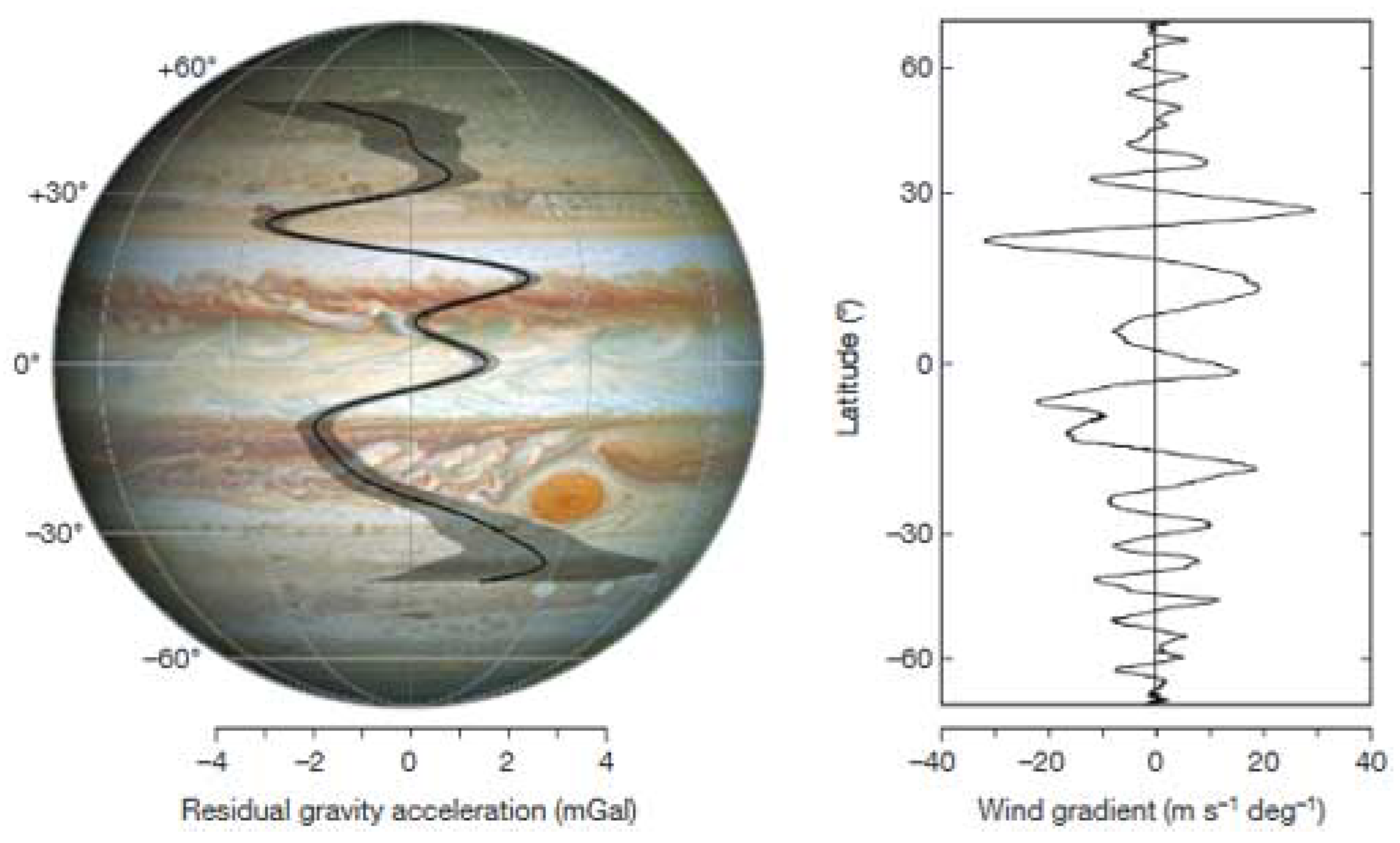
The cells of all living species are regenerating on a periodic basis, for example, 1/3 of hippocampal neurons in humans and mice is exchanged during the lifetime[411] (and neurons represent the worst case - due to their extreme longevity), thus, the cellular regeneration in the Sun should not be surprising, whether it is food or constitutional mass.
Capacity for real mass below the Sun’s surface may be full, but all mass orbiting the Sun may be considered as its real mass. However, it is obviously not fuel mass, rather constitutional or symbiotic mass of the system. The 3rd order period of the Solar System cycle may be related to this mass through the mass barycentre of the system.
I have previously calculated the neutral gravitational mass equivalent for the surface plasma at the equator which would make its angular velocity Keplerian. The source for this energy may be the motion of the barycentre.
In any case, if one assumes that conversion between neutral and electro-magnetic component of the general force of the Sun is also periodic and that such energy replaces fusion reactions in equivalent way, the period of recharge is:
and it is in good agreement with the hypothesized 3rd cycle period (a fraction of mass N = 0.6946847 would yield the hypothesized value - 1512000 years).
In comparison with living beings, one might notice a problem of exhausted fuel - what happens with the ash from fusion reactions (end products of fusion)?
There are couple of solutions:
- the ash is ejected periodically,
- the ash forms the constitutional mass.
Time compression at the ends of Solar System cycles implies gravitational stress of Solar System maxima.
While the 2nd solution may be plausible, at least at the end of one type of the cycles some mass must be ejected out from the Sun. It certainly seems easier than in case of the planets, as unlike the planets, the Sun does not have a solid [real] mantle to block the explosion (although terrestrial planets may be interpreted as Sun’s or Solar System’s mantle, they are in a localized form with plenty of space in between).
The ash content depends on the cycle period, being mostly Helium in smaller cycles but with heavier elements formed in explosions at the end of larger cycles. Helium is probably used to form the core (which should be a Jupiter-like planet).
Rather than being a simple delocalization or a collapse to a different scale, collapse of a graviton can also be a collapse of the 3-dimensional spherical neutral form into a 2-dimensional charged form. Since the surface graviton of the Sun is entangled with Mars’ graviton, with this kind of collapse, two ring maxima would be aligned and the ejection of ionized ash would not be isotropic, rather targeting Mars through the tubes of entanglement (magnetic field lines). The Fe covered surface of Mars may be the evidence for this.
The mass is ejected with a change in spin and since the changes are synchronized, a lot of mass could be absorbed at the moment of inversion when the field on Mars is the weakest.
18.3.1. 1st Order Cycle from Inter-Scalar Time Dilation
It is well known that the lifetime of a star is inversely proportional to its mass. Thus, star lifetime or lifecycle may be derivable from the time-energy uncertainty:
M = star mass
c1 = 2.93 × m/s
But what is the value of ℏ here? In the chapter 12. Quantization of momentum, a ℏ for outer planets (relative to total mass) of ≈ 5 × Js was obtained. From this one can obtain a corresponding ℏ for the Sun:
= Sun mass = 1.988500 × kg
= Jupiter mass = 1898 × kg
= 5 × Js
This gives a T for the Sun of about 15.34 seconds - which is, very interestingly, close to the half-life of 10C (19.3 s) and 11Be (13.76 s). This time is, however, relative to U1 scale. One way to convert it to our scale is, roughly:
c1 = U1 speed of light = 2.93 × m/s
c0 = c = standard speed of light = 2.99792458 × m/s
≈ Moon’s mass = 0.073 × kg
where is the non-dimensional inter-scalar conversion (dilation) factor, here scaled to the Sun from the previously determined relation between human mean lifetime (or lifetime of human neural cells) and the 3rd order period (see chapter 17.2. Age, lifecycle and the 3rd order period) - previously associated with bodies on the order of mass of the Moon or Earth’s inner core (and, thus, with Earth’s graviton cycling, where the 3rd order period should also be equal to the mean lifetime of Earth’s neural cells).
This here is a rough approximation though. Assuming that T1 is a superposition of 10C and 11Be half-lives, its value is 16.53 U1 seconds (for the arithmetic mean), which then results in 4.52 billion years in our time (standard time). It is however, questionable, whether it is appropriate to use half-life here, rather than mean lifetime (log2e × half-life), which would produce a higher value. But is the Moon mass the best value to use? Using Earth’s inner core mass instead (1.1 × kg), with T1 = log2e × 16.53 U1 seconds, one obtains 4.33 billion years.
18.4. As a Living Organ[ism]
Considering the energy output (metabolic rate) of P = 3.8 × W, the standard relation between metabolic rate and mass[412]:
gives 0.86 for the exponent (M = total mass of the sun = 1988500 × 1024 kg). For a mammalian organ this would be between a kidney and a liver[379], suggesting an embryonic stem cell in the process of differentiation.
19. Inflation and Dark Energy
According to CR, observable universe cannot be absolute - if it had a beginning it was a relative beginning and if it was inflated it was inflated from a relative, not absolute, singularity.
The inflation thus did not proceed from a single absolute point, and with inflation of large scale gravitons, effectively, large scale structures could have been inflated as well. Galaxies probably start with the inflation of a supermassive graviton, which afterwards deflates (probably in steps - through discrete energy levels) to a stable [ground] state. In any of these states, graviton may be interpreted as a supermassive black hole. The energy lost with deflation probably consists of gravitons, which then, in similar fashion (inflation/deflation) create planetary systems. Inflation of galaxies and planetary systems may be considered as inflation of universes, even if they have similar properties.
This hypothesis enables a relatively fast evolution of galaxies and planetary systems between equilibrium states, suggesting that one may have to look very far in order to detect large differences between distant and near galaxies.
In any case, the theory implies that masses of very young galaxies should be dominated by central supermassive black holes, while, in developed galaxies, vice versa should be true.
If planetary systems are relative equivalents of standard atoms in a particular state (pressure/temperature) with localized components, observable universe becomes a gas of extremely low density. Dark energy, assuming it is real, is thus simply the energy driving gas expansion due to a gradient in scaled pressure/temperature. Galaxies can then be interpreted as large scale quantum vortices.
Black holes and other living gravitational wells of U1 scale can be understood as large scale vacuum quanta, increasing in strength with inflation and causing contraction of constituent matter, with stretched space (at times of inflation of space, not expansion) between them creating (inflating) new gravitational wells between galaxies.
It seems that dark energy is not stretching space rather creating new space (energy density of space remains constant). This is consistent with gas-like expansion (it doesn’t affect spacetime, the increasing volume of gas simply increases the amount of spacetime contained within the volume), thus, the observable universe should be cooling down. However, expansion should affect large scale gravitons (components of large scale gas) such as the gravitational maxima of black holes. Thus, correlation should exist between dark energy and black hole sizes. If expansion is not slowing down the growth of black holes should be continuous (although probably in oscillating manner).
Indeed, recent analyses support the notion that growth of black holes is proportional to dark energy[415].
The expansion of the observable universe has been questioned before and there are results consistent with a non-expanding, Euclidean universe[416] regarding some phenomena previously considered to favour expanding universe, although none solve all the problems - e.g., increasing redshift with distance or time dilation of distant events.
Some recent analyses suggest that the expansion of the observable universe is not accelerating[417] and the redshift previously used as evidence for acceleration should be attributed to local "bulk flow" instead.
If photons have rest mass, as CR implies, energy can be lost with distance (but it can also be replenished periodically - most likely it oscillates about some mean value but that mean value should not be absolutely constant either). If the mechanism for energy loss from distant galaxies is not scattering of light through interactions with standard (U0 scale) matter, the interactions must be involving smaller scales of photon energy components. These are causing changes in values of momentum relatively independent of wavelength, and without affecting direction significantly. Photons, having rest mass, must have a range - making anything beyond the range invisible. In case of different ranges, this would also affect brightness with distance.
However, even these interactions cannot explain time dilation, which has been observed in Type Ia supernovae[418]. Signatures of time dilation have also been found in gamma-ray bursts but with lower confidence[419]. Thus, unless the speed of time in the observable universe was lower in the past, time dilation must involve expansion. Speed of time should have indeed been lower when the universe was smaller due to higher energy density - but this also implies expansion, and, apart from the early epoch, the difference should be negligible. However, larger gravitons/objects in the past would also imply slower passage of time, without requiring expansion.
In any case, at least the magnitude of the rate of expansion should be questionable. Observations also suggest that small scale effects on photon energy are oscillating with distance - consistent with the hypothesized oscillation of photon mass, which, assuming it involves partial localization/delocalization (rather than simply flavour oscillation), periodically results in acceleration rather than deceleration of photons exclusively. The oscillation must be correlated with properties of space. If there is no significant loss of energy (considering the hypothesized photon mass, this is probably the case), energy of the photon may be kept relatively constant through these interactions.
20. Stability of Elements
Structure of U0 elements seems to be entangled with the configuration of the parent U1 universe. This also makes the stability of isotopes dependent on this configuration.
The stability curve and decay rates of individual isotopes thus may change strongly in transition from one U1 cycle state to another, but the rates should also oscillate in equilibrium.
Stable isotopes are concentrated along this curve:
where N = N0 is the number of neutrons, P = P0 = Z is the number of protons of the isotope and is the maximal number of protons for a stable element (for the Solar and equivalent systems, = 82, corresponding to Pb - lead). is the small shift in value of N due to weak evolution through state lifetime ().
where N1 is the number of neutrons and P1 the number of protons of the parent system - U1.
is the atomic number (number of protons) of the most stable element - element with maximal number of stable isotopes.
is the atomic number of the element lying on the N(P,t) curve with P/N ratio equal to .
For the Solar System, in state 6p4n:
Note that constants C1 and are the same as those determined in chapter 17.2.3. Speed of time.
Figure 33 shows all stable isotopes of the Solar System (green) and the N(P,t) curve (black).
Note the following:
- for t > 1495840 years (t ≈), the isotope lying on the curve with P/N ratio exactly equal to 2/3 is Pt-195 (Platinum, P = 78). The placement of other Platinum isotopes is symmetric relative to the curve,
- for = 0 (t = 3/), the isotope is Pb-205 (Lead, P = 82). At t = 3/ this is a stable isotope. 1/3 of other stable isotopes are above the curve, 2/3 below,
- for t = 4/ the isotope is Hg-200 (Mercury, P = 80). 1/3 of other stable isotopes are above the curve, 2/3 below,
- the ratio of horizontal to vertical distance between Lead-205 and Platinum-195 is (82 - 78) / (123 - 117) = 4/6 = 2/3,
- the ratio of horizontal to vertical distance between Lead-205 and Hg-200 is (80 - 78) / (120 - 117) = 2/3,
- at t ≈, Tin (Sn, P = 50) has the highest number of stable isotopes (10). Tin isotope lying on the curve is Sn-116 (50 protons, 66 neutrons). 2/3 of other stable Tin isotopes is above the curve, 1/3 is below,
- at t ≈, the only elements without stable isotopes are Tc (Technetium, P = 43) and Pm (Promethium, P = 61). The isotopes lying on the curve are Tc-98 and Pm-146. Vertical distance from Sn-116 to Tc-98 is equal to horizontal distance from Sn-116 to Pm-146.
21. Electric Gravity
According to CR, electric and gravitational forces are interchangeable components of general force. This exchange may not be limited to annihilation or vertical mass oscillation events.
Inside the atom, force field between negative and positive charges is neutralized and this electro-magnetic potential may be locally at least partially exchanged with gravitational potential (which may be interpreted as annihilation of entangled field components and increase in gravitational coupling strength).
Thus, a Hill sphere radius (rH) of an atom could be correlated with its charge radius.
This gives, for a Carbon-12 atom with a nucleus mass m = 1.992646883 × kg inside the gravity field of Earth (M = 5.972 × 1024 kg) at R = 6371 km (surface), a radius of:
This is in agreement with the experimentally obtained radius of 70 pm (±5 pm). Calculation for other elements of the periodic table yields similar results.
Note that Hill radii are different for the different isotopes of the same element while the experimentally obtained atomic radii are charge radii and thus independent of the number of neutrons (radius represents the orbit of the outermost electron). In example, for Carbon-14 the obtained value is 69.5 × m, and even closer to 70 pm if one calculates using equatorial radius of Earth instead of the mean volumetric (a possible indicator that the Solar System soul was a part of a 14(C-N-O) cycle in the previous incarnation).
Figure 34 shows experimentally obtained radius (green) and calculated Hill sphere at R = 6371 km (black) for all stable isotopes. Evidently, radii are not only correlated but values of covalent radii oscillate about the Hill radii, confirming the entanglement of U0 and U1.
Comparing data from 1964.[420] and 2008.[421] shows a compression of radii and convergence to Hill radii - such changes are expected in CR (no absolute constants) and these should probably be accelerating as the Solar System approaches the end of the current cycle.
Figure 35 shows the experimentally obtained radius (green squares) and calculated Hill sphere at R = 6371 km (black squares) for isotopes with neutron number adjusted to match the charge radius.
In calculations above, atomic mass has been quantized by u = 1.66053907 × kg (atomic mass constant) with integer number of protons P and neutrons N [m = (P + N) × u] so Hill radii are quantized too. The overlap of Hill radii with charge radii in Figure 35 shows that charge radius is quantized too (there is a number of neutrons N for which the Hill radius will match the charge radius).
Figure 36 shows the number of neutrons N used with each element to obtain a Hill radius equal to charge radius. It seems that minima and maxima here correspond to the elements in the group 18 and group 1, respectively, where the group 1 also belongs to the s-block of the periodic table (the minima thus correspond to noble (inert), monoatomic gases). However, more precisely, the minima correspond to the maxima of ionisation potential (for example, one minima is Hg, which is not a noble gas, but it represents a maximum in ionisation potential of elements). Valence electrons in all these minima are paired and all the outer shells are full. All are probably also diamagnetic. From this, one can conclude that the primary driver of convergence to Hill radii is the annihilation of spin, or the binding of fermions into composite bosons (cobosons). Cobosons are involved in superfluidity and superconductivity, and the higher is the entanglement between the fermions the more bosonic will be their joint nature, and the harder will be to ionize them. Now, the Josephson effect strongly suggests that [at least] in cobosons separated by a non-superconducting barrier the total charge is oscillating between positive and negative values, with the frequency being proportional to the kinetic energy of cobosons. And barriers exist between cobosons in atoms. With the neutralization of electro-magnetic force, orbital radius of paired electrons depends solely on gravity, explaining the convergence to Hill radii. Effectively, the higher the oscillation frequency, the higher is the convergence to Hill radii. But this also implies that much of the electro-magnetic potential or coupling has been exchanged for gravitational - as the standard gravitational coupling (G) is much too low to keep these particles in that orbit, at least assuming non-relativistic masses. However, higher oscillation is correlated with higher kinetic energy and kinetic energy is gravitational mass. Thus, it cannot be ruled out that here the prevailing energy is gravitational, whether in the form of relativistic mass or increased gravitational coupling (as long as bosonic states can be maintained). In any case, gravity and electricity cannot be absolutely decoupled, the question is only how much is an gravity electric or how much is an electricity gravitational.
The higher is the entanglement between paired fermions the more similar is their behaviour to elementary bosons (this makes sense, but can be shown mathematically as well[422]). Per CR, absolute or absolutely elementary bosons cannot exist. Bosons in general then could be electrically neutral, it is only with their decay that the oscillation collapses [or, the kinetic energy transforms] to a particular charge eigenstate.
From the figures above it is obvious that elements (atoms) can be grouped into shells the same way as electrons are grouped within atoms. Grouping is shown in Table 48. There are two interpretations - either the shells L, M and N are doubled or the grouping is reflected after the N shell, so shells O, P and Q contain the same number of elements such as shells N, M and L, respectively. Note that in case of alternative (Og) grouping, no elements beyond Og are theoretically possible - otherwise another shell would be present between He and Li.
Note that no elements beyond Oganesson (Og) have been found (or synthesized) to date, despite numerous attempts. Explanation may indeed lie in the fact that all shells of stability are filled, according to the above.
Gravitational constant G is not dimensionless and therefore not invariant.
On the standard atom scale U0, gravitational constant for a completely neutralized general force can be derived from previously obtained orbital momentum of the Carbon-10 outermost electron (in Solar System equivalent state):
v = v = 5.585837356 × 10⁵ m/s
r = r = 70 × m
where m, v, r are components of the outermost electron orbital momentum (mass, velocity, radius).
If one now, equalizes electric force with gravitational force (for photon/graviton mass > 0 [Yukawa, Proca[423]):
discarding / r factors due to being practically equal and equal to 0 on both sides (expecting large r):
ℏ = reduced Planck’s constant = 1.054573 × Js
c = 2.99792458 × 10⁸ m/s
k0 = Coulomb constant = 8.9875517873681764 × 10⁹ Nm2/C2
Q = electron charge = 1.60217733 × C
= photon mass
Mn = U0 graviton mass
Using previously obtained photon mass = 2 × 9.10938356 × kg and carbon graviton mass Mn = 2 × 1.663337576 × kg in CR, this gives:
as the distance in space when two forces become equal - basically the range of gravity for graviton mass roughly equal to Mn.
As shown previously, components of general force, charge and mass are exchangeable through inflation/deflation of momentum components (even in neutral particles, the amount of gravitational mass can increase at the expense of charge mass, with particle remaining neutral). Nature of the force can thus oscillate.
Taking into account error margins, obtained distance is equal to the radius of the cosmological event horizon of the observable universe. Assuming currently accepted [img] age (13.799 × 10⁹ years), constant speed of light:
This is the distance light from the edges of the observable universe would travel to reach us if this universe would be static, and flat for the photon. In the expanding universe, it is the distance at which the expansion reaches the speed of light (c). The current (proper) radius, which takes expansion into account, is thus, much larger, r. But different interpretation is possible. The proportionality with may not be a coincidence. As the photon expands, the enclosed mass is exerting a force on it (due to homogeneity of the universe, per the shell theorem, the mass beyond the photon radius has no such influence on it). This force will not affect the magnitude of its velocity significantly, rather curve its path (rotate the spin momentum), where the proportional stretching of the path (photon) results in redshift (i.e., gravitational redshift). Thus, the universe is probably at least twice as big as r, but the edge of the universe we are observing is at the radial distance equal to r, only the photon momentum has a significant angular component. The unobservable universe in this interpretation is not expanding faster than c, it is rather outside of the photon range. The two interpretations, however, are not mutually exclusive.
The fact that the obtained distance is equal to the radius of the cosmological event horizon is unlikely a coincidence.
Distance in space here can be interpreted as distance in time and the obtained distance can be interpreted as the time when both forces were unified, after which point gravitational force diverged from electro-magnetic force and started evolving separately on standard scale. This implies that the gravitational constant G is proportional to space curvature (or density/pressure of space).
Divergence is common in evolution but it is also common that it affects only one form of energy - the other remaining relatively constant.
Assuming Coulomb’s constant remained relatively constant, G must have changed scale, either through inflation of neutral gravitons (decreasing space curvature on U0 scale, increasing space curvature on U1 scale) or deflation of neutral gravitons (decreasing space curvature on U0, increasing space curvature on U−1). In some prior divergence event, the Coulomb’s constant likely have changed scale. On any scale then, these changes can be interpreted as exchange of one potential for the other. This implies diverse inversion between adjacent scales (vertical energy levels) - e.g., while on one scale space is contracting, on the other it’s probably expanding, on one scale gravity dominates, on other electro-magnetism, etc.
Gravitons of scale U1 are thus strongly entangled with gravitons of U−1 scale - in other words, U−1 gravitons form the space of U1 gravitons. Similarly, gravitons form the space of U0 gravitons (here though, electro-magnetic force dominates). Standard scale particles (U0 gravitons) can be entangled with U1 and U−1 gravitons, but this entanglement is weak so the two can exist independently of each other - naked curvature (dark matter) is the evidence for this. This weak entanglement may also be interpreted as lazy synchronization. Between strongly entangled scales synchronization is effectively real-time, between weak (or anti-correlated) scales synchronization (in space/time) may never happen. If the observable universe is expanding exponentially, without decreasing energy density, this would suggest that additional energy is dominantly the energy on non-gravitational scales (U0, ). In other words, the observable universe is dominantly feeding on real mass (or expanding space dominated by electro-magnetism). But is the universe expanding at conventionally assumed rates? Photons are U−1 particles and, according to CR, must have mass. Even though they are weakly entangled with U0 particles (intergalactic space is mostly devoid of standard atoms, while it is full of photons) they will still lose energy to particles as these are present in between the atoms, forming their space. Density of particles is decreasing with distance from atoms, however, they will still absorb photon energy, the only question is how much - to what degree are they responsible for the photon redshift? In extreme cases, expansion of a universe can be a complete illusion. Taking into account the scaled extremely low density and temperature of the observable universe (it’s a large scale gas), evidently it is a [part of a] discontinuity, possibly a graviton between layers of, relatively, dense large scale matter.
If its angular velocity is equal to c, it is also a black hole maximum (escape velocity = c) for standard particles.
Thus, light coming from large distances may be the light reflected off of the firewall, providing a window to the past of inner content. This would explain the correlation of apparently spatially separated phenomena (galaxies) - these may not be images of different phenomena separated in space, but one separated in time.
Indeed, given its density, the radius of the observable universe is the Schwarzschild radius, suggesting it is a black hole[424]. Note however, that this would be a black hole [radius] for particles of U−1 scale and larger but not for particles of scale and lower (though it can be the effective black hole for these particles where they are strongly entangled with U0 particles).
A couple of problems exist here for conventional theories.
If the observable universe is a black hole its mass should be concentrated at the singularity. This singularity is supposed to be in the form of a 1-dimensional point (for a non-rotating black hole) or a 2-dimensional ring (for a rotating black hole) - both having 0 volume. However, observable universe is, obviously, volumetric.
Another problem is that the centre of this black hole should be nearby. If that is so, and one allows real volume, this should obviously be a non-rotating black hole.
However, the assumption here is that density beyond the observable universe is much lower (even equal to 0, by conventional absolutism). To resolve the paradoxes, the density beyond the observable universe should be the same as it is inside. If it is the same, we are not living in a large scale black hole. If it is bigger, the problem for conventional theories remains, so the assumption is that density remains the same (equal to critical density, preserving perfectly flat space).
This is what I believe as well, observable universe is a part of a larger structure. But not the infinite one, it is a part of a large scale graviton which at some point is surrounded by higher density mass. Per CR, this implies rotation of the observable universe, which the recent studies are confirming with the observed non-random distribution of galactic spin momenta[425]. The asymmetry even grows with the redshift, consistent with the hypothesis of decoherence - where the spin asymmetry is a consequence of momentum conservation with the collapse/fragmentation of large scale momenta into smaller spin momenta.
This still does not answer the question why is the observable radius of the universe such that with the density it has it would be a black hole if it would be isolated?
The answer is in the photon. If it has mass, it has a range, and if that mass is the mass calculated in CR, that range is roughly equal to the observable universe. With oscillation of mass taken into account, it is equal to observable universe. Now the question becomes, why does the photon has such range (mass) that enclosed density gives a Schwarzschild radius?
Obviously, the answer is - the enclosed mass is the black hole for the photon. Radius of the photon expands as it travels, it collapses only with absorption, but it cannot expand indefinitely as the enclosed mass is dragging it down. At the time the relative event horizon (range) is reached the photon must either collapse locally (localize at the relative event horizon) and form U−1 scale space in the form of a static photon (it remains static until it couples with an U0 scale particle and eventually gets re-emitted) or invert momentum and collapse back towards the point of emission. Given the low density of [U0 particles] in intergalactic space, there’s a significant probability the photon will be effectively reflected back once the range is reached. If the observable universe is expanding slower than the speed of light and energy density remains constant, at some point, some distant objects must become illusions - they are the reflected images of closer objects at times these were younger. Range of a photon (or graviton, in general) thus depends on the density of a relative universe (and pressure, in case of rotating universes). Since that range depends on rest mass as well, density and pressure must be relative as well. Black holes are relative. Speed of information is relative, for a massless carrier particle it would be equal to infinity (its range). Everything is, completely, relative.
What is a static photon?
The average speed of standard photon expansion (radial velocity) should be equal to standard speed of light (c = c0), with dragging by the enclosed mass, its radial velocity is being exchanged for angular velocity. With radial velocity equal to 0, the photon is orbiting enclosed mass at the standard event horizon, with orbital speed equal to the standard speed of light, which is also the Keplerian velocity (escape velocity is c). Such orbiting particles are, in CR, called static particles. Non-coupled static particles are dark matter particles. Note that photons, or gravitons in general, can have different energies and, thus, different ranges. More massive particles will have lower ranges and if these are standard photons or standard gravitons, with radial velocities roughly equal to c, they will orbit roughly at the standard speed of light (c) even if that velocity is not Keplerian for the enclosed mass. The orbital speed can become Keplerian with coupling, when the static particle will exchange some orbital momentum for a more localized (spin) momentum. The orbits of non-coupled static particles (or effective gravitons) are relatively unstable, however, their density will be kept relatively constant with constant replenishment, as long as the system is not losing energy.
Note that static particles can annihilate to particles of larger scale. In this way, dark matter can be converted to ordinary matter. Annihilation of static particles at the relative event horizon is the mechanism for evaporation of black holes, where, due to asymmetry in the pressure of space, the part of energy lost is bigger than the part conserved.
Note that, fixing the gravitational constant to
one obtains this:
where is the vacuum permeability (magnetic) constant and K = 1 C/m.
One can now obtain k and Q for the U1 scale (Solar System):
Using = 6.674 × m3/kgs2 and previously obtained c1 = 2.930445979 × 10⁶ m/s:
Ranges on U1 scale:
Using m1 = 1.02413 × 1026 kg and previously obtained = 1.663337576 × kg, = 9.10938356 × kg, the distance where two forces become equal, r = 1.0059686 × 1062 m ≈ 1 × 1062 m.
Note that, if one fixes m1 to
one obtains this:
where = 1.6726218977 × kg is the mass of the standard proton. This suggests that the proton mass (as well as magnetic permeability) depends on the ratio between gravitational and electro-magnetic force [extremes]. Interestingly, the minimum mass of the oldest surviving primordial black hole is about 1012 kg[426], and it would have the size of a proton[424] (or neutron). Difference between this mass and the mass of a standard proton is equal to the difference in strength between electro-magnetic and gravitational force between a standard proton and electron. This would suggest that neutrons (or proton/electron pairs) are evaporated black holes but with gravitational force (mass) exchanged for electro-magnetic one in the process (without the exchange the mass of a proton would be on the order of 1012 kg).
The evaporation process is not linear. In case of Hawking radiation, the rate of evaporation increases with decreasing mass. The proton or atom radius (roughly), however, probably represents the limit of evaporation of energy on the scale of standard radiation. The proton may still be evaporating, but on smaller scale, which may be hardly measurable from our reference frame.
Note that this can be interpreted as transition between discrete vertical energy levels. According to CR, standard protons do represent such energy level. These levels are relatively stable so the proton may not be evaporating at this point. In any case, equilibrium in CR implies mass oscillation about the level mean (with oscillating energy here being of smaller scale than standard radiation).
Note that the difference in masses between standard electrons (or up/down quarks) and standard photons is on the order of difference in strength between electro-magnetic and gravitational force between electrons and quarks. This then suggests that electrons and quarks are vertically excited photons (or half-photons).
The question then is - are protons still evaporating? If so, they should still be losing mass (or decreasing local G, depending on interpretation) and increasing electro-magnetic strength (making them harder to fuse, among other things) if the exchange is ongoing as well. Indeed, experiments done over time confirm decreasing mass in protons[427] (although oscillation cannot be excluded as well).
Exchange, however, should not have significant impact on neutral atoms (interactions between positive and negative charge) but it should impact interactions between equal charges. Intergalactic space dominated by plasma would be affected as ions would be, over time, pushing each other apart with increasing strength as gravitational attraction is replaced with electro-magnetic repulsion. If, in the process, new energy is being inflated as well (e.g., in the form of particles, forming polarized space of standard ions) this could then provide an alternative explanation for the universe’s expansion (dark energy). Since the rate of this exchange cannot be absolutely constant, it may also explain the change of Hubble constant with distance.
If this exchange is happening on standard scale it is probably happening on other scales as well, e.g., electro-magnetic force could still be exchanging for gravity on U1 scale which would then imply energy inflation on U−1 scale (graviton neutrinos forming space of U1 particles). This would be effectively constrained to galaxies and may explain excess dark matter in them.
If this is happening in stars, however, the effect may be balanced with increased loss of mass due to higher thermal energy of plasma (with increasing electro-magnetic repulsion).
Thus, solar winds may be increasing in strength with time while real mass in stars is effectively being exchanged for img mass (dark matter). The more dark matter there is in stars the less there is fusion fuel. Dark matter should also be present in planets. When not taken into account, this could lead to severe misinterpretation of seismic profiles, especially where multiple gravitational maxima exist (where dark matter should be most concentrated).
22. Relation of G Variation to Sun’s Discontinuities
Equalizing the strength of electric and gravitational force between two free particles (positron and electron), disregarding small mass of carrier particles:
yields the following value for the gravitational constant G:
k0 = 8.9875517873681764 × 10⁹ Nm2/C2
Q = 1.60217733 × C
M = 9.10938356 × kg
In CR, gravitational constant G changes with scale. But it may also be modified with neutralization of EM force, when k0 decreases, while G increases.
This enables the gravitational force to be, in extreme cases, if not periodically, a prevailing force in the atom, rather than EM force.
I have previously calculated G relative to a neutralized 10C atom in Solar System equivalent conditions, assuming Keplerian motion:
v = 5.5550351679 × 10⁵ m/s
r = 70 × m
M = 1.663337576 × kg
where m, v and r are components of the orbital angular momentum of the outermost electron.
Calculated G () is now only 5 orders of magnitude smaller than G required for gravity to be equal in strength to EM force between an electron and a positron.
But instead of G increasing, one may assume that k0 decreases by 5 orders of magnitude, or more precisely by this amount:
I have previously calculated that G1 (U1.G) is 5.731534632 × m3/kgs2, which is, relative to G0 (6.674 × m3/kgs2), an increase of:
which is also the ratio between real mass ≈ M (5.97 × 1024 kg) and img mass = m (6.95 × 10¹⁹ kg) of Earth.
There are multiple possible interpretations:
- the and img mass had the calculated values from the beginning of Earth formation, acquired scale mass (standard atoms) then completely filled the gravitational well ( = ) - this is the shielding interpretation,
- is equal to but img mass ( scale dark matter) was initially roughly equal to the current total mass (M) while real mass was roughly 0, during formation img mass was then mostly exchanged (e.g., through annihilation) for real mass so now the real mass is roughly equal to M,
- img mass remained constant, but was effectively exchanged for real mass (with deflation of the graviton associated with ), settling at the scale/value of .
But what was the initial G of Earth’s graviton before localization, assuming dominance of electro-magnetism?
According to the above, it should have been:
If the Earth’s U1 graviton has been extracted from the Sun, as hypothesized, one can now obtain the radius it would have in the current Sun:
M = img mass of the Sun = 1.988500 × 1030 kg
g = gravity of the maximum = 274 m/s2
The above assumes that, prior to collapse, Earth’s naked graviton mass/gravity were roughly equal to Sun’s mass/gravity. But, with the collapse, the mass was exchanged for the inflation of to G1. Some mass was lost in the process, as expected for a decrease in energy level.
This agrees very well with the hypothesis of entanglement of discontinuities with inner planetary orbitals:
R = Sun radius = 695700 km
= Earth orbital = 149.6 × 10⁶ km
= Mars orbital = 227.92 × 10⁶ km
While Earth’s graviton is not currently in the Sun, the radius should represent an energy level (discontinuity) which could be occupied by gravitons still present in the Sun. The discontinuity (r/R = 0.63) is indeed evident through the profile of rotational velocities of the Sun:
The hypothesis of neurogenesis, assuming pending neurogenesis on Earth and completed neurogenesis on Mars and other terrestrial planets, explains why Earth is the only one with an active surface magnetic dipole. The connection of tachocline with 0.63R discontinuity would suggest:
- its position is not permanent and it moves between discontinuities, corresponding to the planet with ongoing neurogenesis,
- possible multiple active discontinuities and associated tachoclines in the past, initially at maximum, or
- current position is the place of birth of all planetary embryos (cores).
The 2nd hypothesis here is most plausible - the tachocline is active as long as the magnetic dipole of the corresponding planet is active (the two phenomena are synchronized).
However, if the tachocline is localized to 0.71R[429] and distance between the tachocline and the discontinuity is scaled from Earth (distance between the charge radius and gravitational maximum), the associated discontinuity is at:
which would be a discontinuity associated with Venus.
In that case the tachocline is the location of a charge radius associated with a 0.5R gravitational maximum and, assuming equal g-factor, such charge radius should also be located at:
In this case though, the g-factor of a neutron might be more appropriate, yielding r = 1.111507303 × 10⁶ km (and a mirror at 444533.257 km = 0.639R).
Note that the 0.71R tachocline is 3/4 of 0.94R, which according to Figure 37 seems to be another discontinuity or a fossilized initial Sun radius.
Above this discontinuity is the tachocline (transition region between the radiative and convective layer of the Sun).
Such fossil is also visible at 0.75R, which should be a discontinuity in 4p6n state.
The 0.63R (2/3 of 0.94R) is also a fossil, as the current location associated with Earth is 0.66R.
Note that 0.63R discontinuity is, similarly to 0.4R (2/5 R) discontinuity, weak (unstable) - it may not always be present in the rotational profile of the Sun.
The 0.63R has been revealed in seismic analysis (periodic, 1.3y signal), and possibly the 0.4R discontinuity too (noted as a low significance bump in rotation variability between 0.2R and 0.6R)[430].
Sun’s GM product has increased 6% due to relativistic energy, so the initial radius at 0.94R implies that the surface radius changes proportionally:
for previously obtained c1 = 2.93 × 10⁶ m/s and v = vs + vp = 996 km/s, gives R0 = 654271.142 km = 0.94 R.
Note 1:
This is analogous to the decrease of Bohr radius due to relativistic mass of the electron. Bohr radius:
using relativistic mass:
It follows:
Here, however, the radius of the atom is decreasing with the relativistic mass of electron, while the radius of the nucleus must increase with the relativistic mass of the gravitational maximum.
Note 2:
Although GM changes proportionally to R, differential rotation can shift discontinuities. Effectively, for the polar regions of the Sun, change is proportional with R2:
This gives R0 = 0.97 R, and, according to Figure 37, it is indeed the correct value for polar regions. Note that the same discontinuity (0.97 R) can be obtained is one assumes that the gravity of the Sun’s surface graviton is invariant to changes in energy levels. In that case, without the accumulated kinetic energy, radius of the Sun decreases to 0.97 R. Note that, taking the shift of 0.03 R into account, 0.63 R discontinuity becomes 0.66 R.
Note also that orbits of planets have been shifted equally, probably as shown in Table 49.
The Earth had thus moved from 0.63 rM to 0.66 rM, while Venus moved equally but in opposite direction, from 0.5 to 0.47. Mars moved from 0.97 to 1 rM and Mercury too moved accordingly.
23. Gyro-Magnetic Ratio and Its Correlation with Earth/Moon
The gyro-magnetic ratio of a particle is the ratio of its magnetic moment to its angular momentum:
With the assumption that mass and charge have equal momentum:
where q, m are charge and mass of the particle, respectively.
Measurements show that this is not valid for quantum particles such as electron. Thus, a dimensionless factor ge (g-factor) was introduced:
The factor has been attributed to quantum effects which do not exist in classical (intuitive) reality - point particles with intrinsic magnetic moment (no rotation). The notion of point particles having any properties is in itself problematic, let alone existence of different point particles with different properties. However, if such particles could exist, due to scale invariance, they would have to exist on bigger scales too. No such thing has ever been observed in reality - all magnetic fields are produced by moving charges of objects having a real radius. Thus, intrinsic magnetic momentum is not intuitive, but intrinsic rotation of charge (producing the momentum) at finite radius greater than 0 is.
In CR there is also no absolutely intrinsic coupling of matter and gravity, and since charge field is a polarized gravitational field, the g-factor can be explained simply by the difference in distribution (or angular momenta) of gravitational mass and charge mass within the particle, preserving the intuitive concepts of reality. Complete relativity not only allows speeds faster than light (information carrier mass is scale dependent) but implies such speeds must exist at some scale, thus the required superluminal rotation of charge (implied at certain radii) in particles such as an electron is not an issue either.
The absolute (invariant) speed limit is not a dimensionless constant and thus is counter-intuitive in complete relativity, but, in this case, the required speed would be valid even in the context of General Relativity (charge is at rest relative to rotating space) if it would incorporate relative scale invariant curvature of space.
Magnetic moment µ and angular momentum L:
where vc, rc are the charge orbital velocity and radius, respectively, and vM, rM are the mass orbital velocity and radius, respectively.
The factor ge is thus:
Being dimensionless, it should be scale invariant relative to particle flavour. This means that the value of ge for electron and positron is equal to ge of Earth, as Earth is a large scale Dirac fermion equivalent (obviously not a point particle unless taken relatively).
Assuming such initial conditions where charge radius is in the outer core (current conditions represent fossilized initial conditions) where gravity was equal to gc = 137 m/s2 and gravitational mass radius was roughly the current inner core radius gM (274 m/s2 gravity), with equal rotation period (and angle between v and r vectors):
Note that it was assumed that mass is not a homogeneous solid body with radius rM but, like the charge, a particle or a stream of particles concentrated in a ring of radius rM. This should be true for initial conditions, although in reality the mass is never concentrated in a ring rather a tube and the momenta are not perfectly synchronized so the g-factor is a bit larger than 2.
Figure 38.
Mass and charge radii of charged bodies.
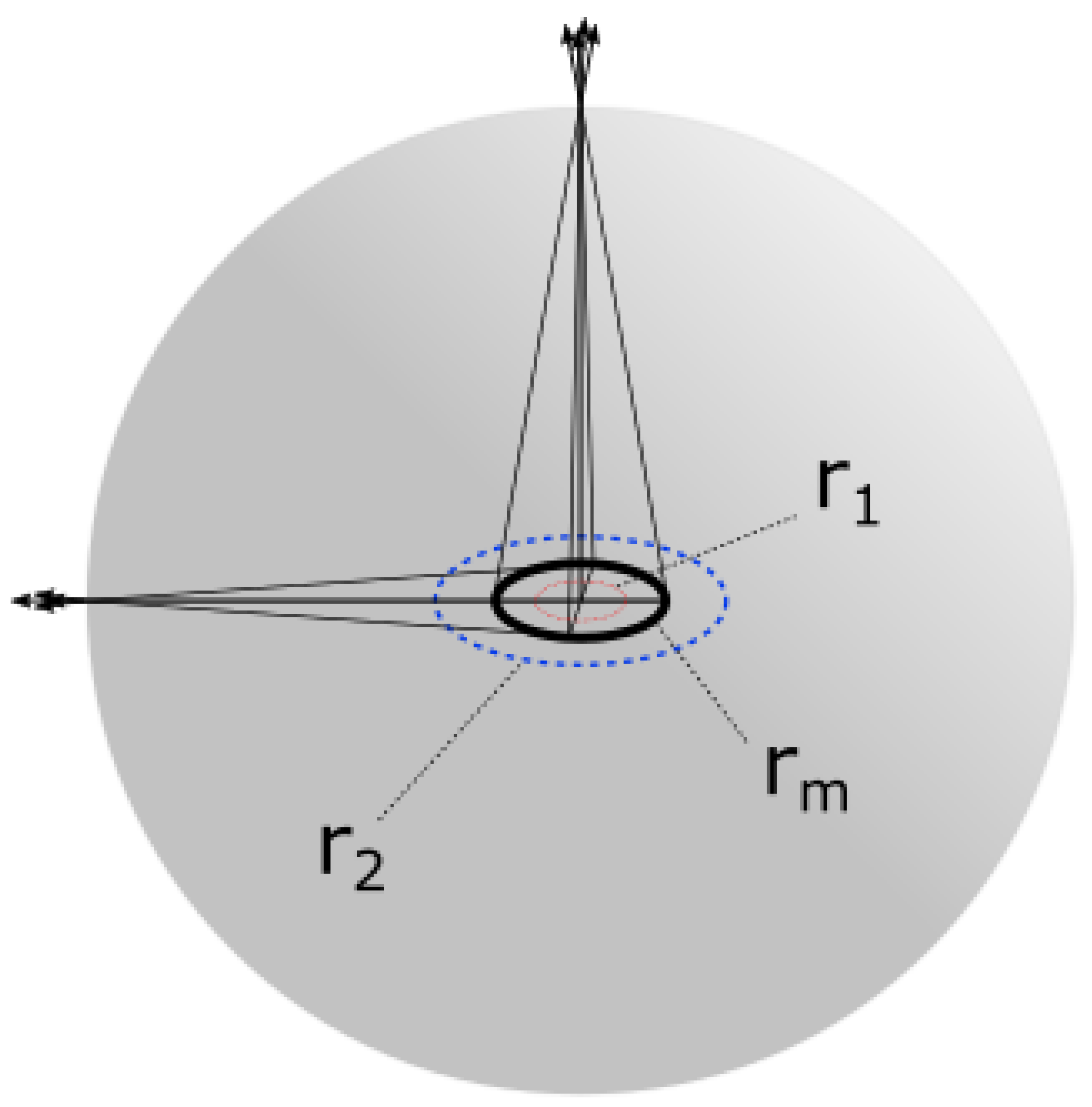
Gravitational acceleration at any point here is a vector sum of accelerations induced by vacuum quanta forming the ring:
In case of equatorial and polar gravity vector components parallel to surface cancel out. Equatorial gravity is thus:
where is the equatorial radius.
Polar gravity:
where is the polar radius.
Deriving the G0M0 product with equatorial gravity fixed to 9.798 m/s2 and calculating polar gravity, for n >= 5, gives 9.34 m/s2. This is smaller than the measured current gravity, so the Earth must be a composite of multiple particles on different energy levels - assuming that, with mass redistribution, the initial state of outer gravity didn’t change.
Note that, here, mass redistribution also involves the transformation of the ring-like form of gravitons into spherical form.
With 2 particles in the local s shell the spin momentum would be 0, so the 3rd particle in another shell is required to explain the Earth’s magnetic moment. This is a different shell so the spin momentum won’t be aligned with any of the two other particles, however, the angle cannot be arbitrary as the value of the spin momentum projection on the quantization axis is fixed. This is shown in Figure 39.
The spins are deflected from the equator by this angle:
The two shells (orbitals) are thus separated by 2 × 35.2643896827547∘ = 70.5287793655094∘ (or 109.47∘, depending on perspective).
Note that the two magnetic dipoles on Jupiter seem to be separated by this angle (see chapter 15.2. validation). This does not imply 3 particles. It can be also explained by the 1e state, where the source of the magnetic momenta are the constituent charges of a single particle. This can be correlated with the hybridization of local s and p orbitals into sp3 orbitals, where the orbitals are separated by 109.47∘ (180∘ - 109.47∘ = 70.53∘), or 109∘28’[431].
Confirmation of this configuration of Earth comes from the state of the Moon (Luna) and non-alignment of Earth’s north and south magnetic poles. Initial obliquity of the Luna relative to Earth’s equator was probably equal to 23.44∘ + 5.14∘ + 6.68∘ = 35.26∘, which is apparently equal to .
One would have to be very ignorant in order to accept all this as coincidence. Thus, the Earth-Moon system is a system of 3 particles (fermions), where 2 equal charges (positrons, according to the chapter 13.1.2. Standard model) exist in Earth as a coboson, while the 3rd (anti-down quark) was initially in the Moon (when it had a magnetic field). However, the Moon’s magnetic field is lost, suggesting that only two components of this particle now exist in the Moon, while the 3rd one has been absorbed by Earth - when the magnetic field on Earth has been established.
Thus, with the assumption of 3 components per particle, there are 7 components of the 3 particles in Earth, 2 in Luna. The initial 6 components may be correlated with the 6 layers of the Earth’s neocortex (but also with the carbon configuration of the system), with the added 7th one correlated with the development of the 7th layer (which has been already hypothesized). However, 7 components may be correlated with 7 discontinuities instead, and thus, indirectly, with 6 layers in between.
It appears that, in the collapse, 6.68∘ of Luna’s obliquity to Earth’s equator has been exchanged for obliquity to Luna’s own orbital plane. Now, if another component of the Moon collapses into Earth, the magnetic field on the Moon could be restored, while the Earth’s magnetic field would collapse (although not completely, at least if the Moon’s graviton remains in orbit).
Note that all this suggests that the Moon currently does not significantly contribute to the generation of the Earth’s magnetic field after all, but it is correlated with it. Initially, however, the Moon has not only generated its own magnetic field but was inducing a significant magnetic field in Earth (similar to how the motion of an standard electric charge in a loop induces a magnetic field in the centre).
The components of Earth’s particles may not be correlated solely with Earth’s neurogenesis, the configuration is probably directly or indirectly correlated with neurogenesis in standard mammals on Earth. The sparse neuron cell population of the layer I may indicate an underdeveloped layer, something that could change - correlated with the future absorption of one Moon component.
It cannot be ruled out that this component due to entanglement with local components already affects the brain development in mammals. Since the distance to the Moon is variable, the effect could vary with this distance as well.
Perhaps a Moon in perigee at the time of formation of a particular brain layer would increase the number and/or complexity of neurons in that layer. But the Earth is not entangled only with the Moon, it is entangled with other planets and the Sun as well. Perhaps the astrology then could be based on science, even though the modern Western astrology is not.
Interesting is the fact that we have 5 vital organs, while 5 neurogenesis events have occurred on Earth. Are we going to develop an additional vital organ with the current event? Perhaps the 6th sense that some already have is a precursor to this.
24. Conclusion
The analyses done in the paper, across various interpretations, provide very strong evidence, not only that the Solar System is a localized and vertically excited (large scale) quantum system, but that planetary systems in general represent large scale quantum systems.
Analyses also show that planets such as Earth are relative living beings. High correlation of Earth’s mantle layers with major extinction events is a solid evidence for planetary neurogenesis, or at least for a progenitor or precursor of it (from which neurogenesis evolves). The existence of a discontinuity at 100 km depth even suggests that the formation of a mantle discontinuity precedes surface extinction. This shows that surface extinctions are coded events, which, however, is not surprising for a neurogenesis of an evolving life-form (one would expect for a brain layer to be at least roughly formed before neurons migrate to that layer).
Some questions remain, however, and there are predictions and hypotheses that require additional experiments and observation to be confirmed or refuted.
References
- Complete Relativity: Nature of observables (2024), Amenoum. http://amenoum.byethost17.com/complete_relativity.html.
- NASA Planetary Fact Sheets. https://nssdc.gsfc.nasa.gov/planetary/factsheet/.
- Hadronic uncertainties versus new physics for the W boson mass and Muon g-2 anomalies (2023), P. Athron et al., Nat Commun 14, 659. [CrossRef]
- Images of planets (2013), OpenClipart-Vectors. https://pixabay.com/users/openclipart-vectors-30363/.
- Electron dynamics in the ground state of a laser-generated carbon atom (2013), H. Hultgren et al., Phys. Rev. A 87(3), 031404(R). [CrossRef]
- Six transiting planets and a chain of Laplace resonances in TOI-178 (2020), A. Leleu et al. [CrossRef]
- Multidecadal variation of the Earth’s inner-core rotation (2023), Y. Yang and X. Song, Nature Geoscience 16, 182-187. [CrossRef]
- Large-scale chaos in the solar system (1994), J. Laskar, Astronomy and Astrophysics 287(1), L9-L12. https://adsabs.harvard.edu/full/1994A%26A..287L..9L.
- CODATA recommended values (2018), NIST. https://physics.nist.gov/cuu/pdf/all_2018.pdf.
- What are binary stars? (2023), Space, last access 2025.01.20. https://www.space.com/22509-binary-stars.html.
- Binary stars are all around us, new map of solar neighborhood shows (2021), R. Sanders, last access 2025.01.20. https://news.berkeley.edu/2021/02/22/binary-stars-are-all-around-us-new-map-of-solar-neighborhood-shows/.
- Embedded binaries and their dense cores (2017), S. I. Sadavoy and S. W. Stahler, Monthly Notices of the Royal Astronomical Society 469(4), 3881–3900. [CrossRef]
- The Case for an Early Solar Binary Companion (2020), A. Siraj and A. Loeb, ApJL 899(2), L24. [CrossRef]
- Complete Relativity: Nature of observables (2022), Amenoum. http://amenoum.byethost17.com/complete_relativity.html#tag_determination_of_c_n.
- Dipole Anisotropy in the COBE Differential Microwave Radiometers First-Year Sky Maps (1993), A. Kogut et al., Ap J 419, 1-6. [CrossRef]
- On the Shoulders of Giants: Properties of the Stellar Halo and the Milky Way Mass Distribution (2014), P. R. Kafle et al., ApJ 794(1), 59. [CrossRef]
- Recent advances in the determination of some Galactic constants in the Milky Way (2017), J. P. Vallée, Astrophys Space Sci 362, 79. [CrossRef]
- Putovanje kroz vrijeme (2021), Amenoum. http://amenoum.byethost17.com/log/31_putovanje_kroz_vrijeme.html.
- A dynamical calibration of the mass–luminosity relation at very low stellar masses and young ages (2005), L. M. Close et al., Nature 433, 286-289. [CrossRef]
- Evidence of a Substellar Companion to AB Dor C (2019), J. B. Climent et al., The Astrophysical Journal Letters 886(1). [CrossRef]
- The EBLM project III. A Saturn-size low-mass star at the hydrogen-burning limit (2017), A. von Boetticher et al., Astronomy and Astrophysics 604, L6. [CrossRef]
- WISE J072003.20-084651.2B is a Massive T Dwarf (2019), T. J. Dupuy et al., The Astronomical Journal 158(5). [CrossRef]
- Theoretical mass loss rates of cool main-sequence stars (2006), V. Holzwarth and M. Jardine, Astronomy and astrophysics 463(1), 11-21. [CrossRef]
- Mass loss from active dwarf stars (1996), D. J. Mullan. https://adsabs.harvard.edu/full/1996ASPC.109.461M.
- Jupiter Mass Binary Objects in the Trapezium Cluster (2023), S. G. Pearson and M. J. McCaughrean. https://arxiv.org/pdf/2310.01231.pdf.
- New Post-DART Collision Period for the Didymos System: Evidence for Anomalous Orbital Decay (2023), T. Gudebski et al. [CrossRef]
- Surprise – Again! Asteroid Bennu Reveals its Surface is Like a Plastic Ball Pit (2022), NASA. https://www.nasa.gov/missions/surprise-again-asteroid-bennu-reveals-its-surface-is-like-a-plastic-ball-pit/.
- Journey through future: Evidence of general precursor events (2023), Amenoum. http://amenoum.byethost17.com/log/16_evidence_of_precursor_events.html.
- Density of asteroids (2012), B. Carry, Planetary and Space Science 73(1), 98-118. [CrossRef]
- Giant Planets (2007), T. Guillot and D. Gautier, Treatise of Geophysics 10, Planets and Moons, G. Schubert, T. Spohn (Ed.) (2007), 439-464. [CrossRef]
- Tidal heating of terrestrial extrasolar planets and implications for their habitability (2008), B. Jackson et al., Monthly Notices of the Royal Astronomical Society 391(1), 237-245. [CrossRef]
- A resonant sextuplet of sub-Neptunes transiting the bright star HD 110067 (2023), R. Luque et al., Nature 623, 932-937. [CrossRef]
- Binary asteroid (31) Euphrosyne: ice-rich and nearly spherical (2020), B. Yang et al., Astronomy and Astrophysics 641, A80. [CrossRef]
- Neutrino mass in cosmology: status and prospects (2011), Y. Y. Y. Wong. [CrossRef]
- Probabilistic forecasting of the masses and radii of other worlds (2016), J. Chen and D. Kipping, The Astrophysical Journal 834(1). [CrossRef]
- The Extrasolar Planets Encyclopaedia: Catalogue of Exoplanets (2023), last access 2023.11.27. https://exoplanet.eu/catalog/.
- Atomic Screening Constants from SCF Functions (1963), E. Clementi and D. L. Raimondi, J. Chem. Phys. 38, 2686-2689. [CrossRef]
- Atomic Shielding Constants (1930), J. C. Slater, Phys. Rev. 36 (1), 57-64. [CrossRef]
- DESI dark energy time evolution is recovered by cosmologically coupled black holes (2024), K. S. Croker et al., JCAP10 2024, 094. [CrossRef]
- Rest mass of photon on the surface of matter (2020), M. Goray et al. [CrossRef]
- An Electroweak model with electrons of opposite helicities carrying the same quantum numbers (1981), W. B. Yeung.
- The orbit and stellar masses of the archetype colliding-wind binary WR 140 (2021), J. D. Thomas et al., Monthly Notices of the Royal Astronomical Society 504(4), 5221-5230. [CrossRef]
- Dust Rings in the Wolf-Rayet 140 System (2022), NASA, last access 2025.02.05.
- Dynamic Imprints of Colliding-wind Dust Formation from WR 140 (2025), E. P. Lieb et al., ApJL 979(1), L3. [CrossRef]
- Terminal velocities of Wolf–Rayet winds from infrared He I lines (1994), P. R. J. Eenens and P. M. Williams, Monthly Notices of the Royal Astronomical Society 269(4), 1082-1098. [CrossRef]
- The Great Wave: Evidence of a large-scale vertical corrugation propagating outwards in the Galactic disc (2024), E. Poggio et al. [CrossRef]
- S62 on a 9.9 yr Orbit around SgrA* (2020), F. Peißker et al. [CrossRef]
- A geometric distance measurement to the Galactic Center black hole with 0.3% uncertainty (2019), R. Abuter et al. [CrossRef]
- S62 and S4711: Indications of a Population of Faint Fast-moving Stars inside the S2 Orbit—S4711 on a 7.6 yr Orbit around Sgr A* (2020), F. Peißker et al. [CrossRef]
- On the Formation of Compact Stellar Disks around Sagittarius A* (2008), M. Wardle et al. [CrossRef]
- A supermassive black hole in the early universe growing in the shadows (2023), L. J. Furtak et al. [CrossRef]
- Evidence for heavy-seed origin of early supermassive black holes from a z ≈ 10 X-ray quasar (2024), Á. Bogdán et al., Nature Astronomy 8, 126–133. [CrossRef]
- Broad-Line AGN at 3.5<z<6: The Black Hole Mass Function and a Connection with Little Red Dots (2024), A. J. Taylor et al., preprint [arXiv]. [CrossRef]
- The Rise of Faint, Red AGN at z>4: A Sample of Little Red Dots in the JWST Extragalactic Legacy Fields (2025), D. D. Kocevski et al., preprint [arXiv]. [CrossRef]
- Constraints on stupendously large black holes (2020), B. Carr et al., Monthly Notices of the Royal Astronomical Society 501(2), 2029-2043. [CrossRef]
- Tripling the Census of Dwarf AGN Candidates Using DESI Early Data (2025), R. Pucha et al., ApJ 982(1), 10. [CrossRef]
- JADES Ultrared Flattened Objects: Morphologies and Spatial Gradients in Color and Stellar Populations (2024), J. L. Gibson et al., ApJ 974(1), 48. [CrossRef]
- Lifetimes of interstellar dust from cosmic ray exposure ages of presolar silicon carbide (2020), P. R. Heck et al., Proc. Natl. Acad. Sci. U.S.A. 117(4), 1884-1889. [CrossRef]
- The accelerations of stars orbiting the Milky Way’s central black hole (2000), A. M. Ghez et al., Nature 407, 349–351. [CrossRef]
- Stellar orbits near Sagittarius A* (2002), A. Eckart et al., Monthly Notices of the Royal Astronomical Society 331(4), 917-934. [CrossRef]
- The Sun and stars as the primary energy input in planetary atmospheres (2010), I. Ribas, Proceedings of the International Astronomical Union 5(S264), 3-18. [CrossRef]
- Stellar Multiplicity (2013), G. Duchêne and A. Kraus, Annual Review of Astronomy and Astrophysics 51, 269-310. [CrossRef]
- Evidence of hydrogen-helium immiscibility at Jupiter-interior conditions (2021), S. Brygoo et al., Nature 593(7860), 517-521. [CrossRef]
- A diffuse core in Saturn revealed by ring seismology (2021), C. R. Mankovich and J. Fuller, Nature Astronomy 5, 1103–1109. [CrossRef]
- The Orbit of Planet Nine (2021), M. E. Brown and K. Batygin, The Astronomical Journal 162(5). [CrossRef]
- The Curiously Warped Mean Plane of the Kuiper Belt (2017), K. Volk and R. Malhotra, The Astronomical Journal 154(2). [CrossRef]
- Evidence of controversial Planet 9 uncovered in sky surveys taken 23 years apart (2025), Space, last access 2025.05.23. https://www.space.com/astronomy/solar-system/evidence-of-controversial-planet-9-uncovered-in-sky-surveys-taken-23-years-apart.
- A Search for Planet Nine with IRAS and AKARI Data (2025), T. L. Phan et al., preprint [arXiv]. [CrossRef]
- Pluto and Beyond (2014), M. D. Lemonick, Scientific American 311(5), 46-53. [CrossRef]
- A bright triple transient that vanished within 50 minutes (2023), E. Solano et al. https://arxiv.org/pdf/2310.09035.pdf.
- Asymptotic g modes: Evidence for a rapid rotation of the solar core (2017), Fossat et al. [CrossRef]
- The First VERA Astrometry Catalog (2020), T. Hirota et al., Publications of the Astronomical Society of Japan 72(4), 50. [CrossRef]
- Amenoum (2024), Amenoum. http://amenoum.byethost17.com/authors/Amenoum.html.
- Solution to gravitational anomalies: Reincarnation and karma of consciousness (2023), M. Ljubičić (Amenoum). http://amenoum.byethost17.com/log/7_solution_to_gravitational_anomalies.html.
- Micrometeoroid infall onto Saturn’s rings constrains their age to no more than a few hundred million years (2023), S. Kempf et al., Science Advances, 9(19). [CrossRef]
- Measurement and implications of Saturn’s gravity field and ring mass (2019), L. Iess et al., Science, 364(6445). [CrossRef]
- Evidence suggesting that earth had a ring in the Ordovician (2024), A. G. Tomkins et al., Earth and Planetary Science Letters 646, 118991. [CrossRef]
- Long-term patterns of body mass and stature evolution within the hominin lineage (2017), M. Will et al. [CrossRef]
- Cosmogenic radionuclides reveal an extreme solar particle storm near a solar minimum 9125 years BP (2022), C. I. Paleari et al. [CrossRef]
- On the Origins of Magnetic Excursions in the Great Lakes (1981), W. F. Kean. [CrossRef]
- The Norwegian-Greenland Sea, the Laschamps, and the Mono Lake Excursions Recorded in a Black Sea Sedimentary Sequence Spanning From 68.9 to 14.5 ka (2020), J. Liu et al. [CrossRef]
- The Lake Mungo geomagnetic excursion (1976), M. F. Barbetti and M. W. McElhinny. [CrossRef]
- The 26.5 ka Oruanui eruption New Zealand: an introduction and overview (2001), C. J. N. Wilson. [CrossRef]
- Robust Characteristics of the Laschamp and Mono Lake Geomagnetic Excursions: Results From Global Field Models (2019), M. Korte et al. [CrossRef]
- Evidence for two intervals of enhanced 10Be deposition in Antarctic ice during the last glacial period (1987), G. M. Raisbeck et al. [CrossRef]
- Late Pleistocene geomagnetic excursion in Icelandic lavas: confirmation of the Laschamp excursion (1990), S. Levi et al. [CrossRef]
- The Toba supervolcano eruption caused severe tropical stratospheric ozone depletion (2021), S. Osipov et al. [CrossRef]
- The Gothenburg Magnetic Excursion (1977), N. Mörner. http://dx.doi.org/10.1016/0033-5894(77)90031-X.
- Evidence for an extraterrestrial impact 12900 years ago that contributed to the megafaunal extinctions and the Younger Dryas cooling (2007), R. B. Firestone et al. [CrossRef]
- A global environmental crisis 42,000 years ago (2021), A. Cooper et al., Science 371(6531), 811-818. [CrossRef]
- On the Precession as a Cause of Pleistocene Variations of the Atlantic Ocean Water Temperatures (1966), E. P. J. van den Heuvel, Geophysical Journal International 11(3), 323-336. [CrossRef]
- Orbital and millennial-scale features of atmospheric CH4 over the past 800,000 years (2008), L. Loulergue et al., Nature 453, 383-386. [CrossRef]
- The 13 million year Cenozoic pulse of the Earth (2015), J. Chen. [CrossRef]
- When and Why Did Human Brains Decrease in Size? A New Change-Point Analysis and Insights From Brain Evolution in Ants (2021), J. M. DeSilva et al. [CrossRef]
- On the 1470-year pacing of Dansgaard-Oeschger warm events (2002), M. Schulz. [CrossRef]
- Estimating the Date of Earth Overshoot Day 2023 (2023), Global Footprint Network. https://www.overshootday.org/content/uploads/2023/06/Earth-Overshoot-Day-2023-Nowcast-Report.pdf.
- MIT Predicted in 1972 That Society Will Collapse This Century. New Research Shows We’re on Schedule. (2021), A. Nafeez, Vice, access time 2023.10.19. https://www.vice.com/en/article/z3xw3x/new-research-vindicates-1972-mit-prediction-that-society-will-collapse-soon.
- July Temperature Update: Faustian Payment Comes Due (2021), J. Hansen and M. Sato. http://www.columbia.edu/~mhs119/Temperature/Emails/July2021.pdf.
- Figure SPM.8 in IPCC 2021: Summary for Policymakers (2021), IPCC. https://dx.doi.org/10.1017/9781009157896.001.
- Geomagnetic reversals from impacts on the Earth (1986), R. A. Muller and D. E. Morris, Geophysical Research Letters 13(11), 1177-1180. [CrossRef]
- A Causality Problem for Milankovitch (2000), D. B. Karner and R. A. Muller, Science 288(5474), 2143-2144. [CrossRef]
- Sun-like stars produce superflares roughly once per century (2024), V. Vasilyev et al., Science 386(6727), 1301-1305. [CrossRef]
- On some characteristics of large kinetic energy coronal mass ejections during 1996–2015 (2018), N. Mittal and V. K. Verma, New Astronomy 63 6-14. [CrossRef]
- A history of solar activity over millennia (2023), I. G. Usoskin, Living Rev Sol Phys 20, 2. [CrossRef]
- The Relationship of Sunspot Cycles to Gravitational Stresses on the Sun: Results of a Proof-of-Concept Simulation (2011), D. Jassby. [CrossRef]
- Near-collapse of the geomagnetic field may have contributed to atmospheric oxygenation and animal radiation in the Ediacaran Period (2024), W. Huang et al., Commun Earth Environ 5, 207. [CrossRef]
- The solar dynamo begins near the surface (2024), G. M. Vasil et al., Nature 629, 769–772. [CrossRef]
- Internal rotation of Sun (2010), SOHO. https://ase.tufts.edu/cosmos/view_picture.asp?id=1368.
- Velocity Curves for Spiral Galaxies (2015), C. R. Nave. http://hyperphysics.phy-astr.gsu.edu/hbase/Astro/velcurv.html.
- Discovery of variation in Solar coronal rotation with altitude (2001), H. O. Vats et al.
- Up-, down-, strange-, charm-, and bottom-quark masses from four-flavor lattice QCD (2018), A. Bazavov et al., Phys. Rev. D 98, 054517. [CrossRef]
- Framework for the architecture of exoplanetary systems (2023), L. Mishra et al. https://arxiv.org/pdf/2301.02374.pdf.
- A million binaries from Gaia eDR3: sample selection and validation of Gaia parallax uncertainties (2021), K. El-Badry et al., Monthly Notices of the Royal Astronomical Society 506(2), 2269–2295. [CrossRef]
- A Quantum-Like Description of the Planetary Systems (2007), F. Scardigli. [CrossRef]
- Self-Organizing Systems in Planetary Physics: Harmonic Resonances of Planet and Moon Orbits (2018), M. J. Aschwanden. [CrossRef]
- The Venusian Environment (2001), F. W. Taylor et al., last access 2024.10.17. https://api.semanticscholar.org/CorpusID:9606507.
- The Gutenberg Discontinuity: Melt at the Lithosphere-Asthenosphere Boundary (2012), N. Schmerr, Science 335(6075), 1480-1483. [CrossRef]
- Mercury’s Hidden Past: Revealing a Volatile-dominated Layer through Glacier-like Features and Chaotic Terrains (2023), J. Alexis P. Rodriguez et al., Planet. Sci. J. 4(11), 219. [CrossRef]
- Saturnian Rings Fact Sheet (2022), NASA, last access 2024.10.05. https://nssdc.gsfc.nasa.gov/planetary/factsheet/satringfact.html.
- Neptunian Rings Fact Sheet (2015), NASA, last access 2024.10.05. https://nssdc.gsfc.nasa.gov/planetary/factsheet/nepringfact.html.
- Neptunian Satellite Fact Sheet (2024), NASA, last access 2024.10.05. https://nssdc.gsfc.nasa.gov/planetary/factsheet/neptuniansatfact.html.
- The Orbits of the Inner Uranian Satellites from Hubble Space Telescope and Voyager 2 Observations (1998), R. A. Jacobson, AJ 115(3), 1195. [CrossRef]
- The Second Ring-Moon System of Uranus: Discovery and Dynamics (2006), M. R. Showalter and J. J. Lissauer, Science 311(5763), 973-977. [CrossRef]
- Uranian Satellite Fact Sheet (2023), NASA, last access 2024.10.05. https://nssdc.gsfc.nasa.gov/planetary/factsheet/uraniansatfact.html.
- Measurement and implications of Saturn’s gravity field and ring mass (2019), L. Iess et al., Science 364(6445), eaat2965. [CrossRef]
- Saturn’s dynamic D ring (2007), M. M. Hedman et al., Icarus 188(1), 89-107. [CrossRef]
- Extensive Spiral Corrugations (2011), CICLOPS, last access 2024.10.05. https://ciclops.org/view/5722/Extensive_Spiral_Corrugations.html.
- Corrugations and eccentric spirals in Saturn’s D ring: New insights into what happened at Saturn in 1983 (2015), M. M. Hedman et al., Icarus 248, 137-161. http://dx.doi.org/10.1016/j.icarus.2014.10.021.
- Neptune Fact Sheet (2024), NASA, last access 2024.10.08. https://nssdc.gsfc.nasa.gov/planetary/factsheet/neptunefact.html.
- Uranus Fact Sheet (2024), NASA, last access 2024.10.08. https://nssdc.gsfc.nasa.gov/planetary/factsheet/uranusfact.html.
- Saturn Fact Sheet (2024), NASA, last access 2024.10.08. https://nssdc.gsfc.nasa.gov/planetary/factsheet/saturnfact.html.
- Jupiter Fact Sheet (2024), NASA, last access 2024.10.08. https://nssdc.gsfc.nasa.gov/planetary/factsheet/jupiterfact.html.
- Eccentricity of the geomagnetic dipole caused by lopsided inner core growth (2012), P. Olson et al. [CrossRef]
- Earth Fact Sheet (2024), NASA, last access 2024.10.09. https://nssdc.gsfc.nasa.gov/planetary/factsheet/earthfact.html.
- Mercury Fact Sheet (2024), NASA, last access 2024.10.09. https://nssdc.gsfc.nasa.gov/planetary/factsheet/mercuryfact.html.
- The deep Earth may not be cooling down (2016), D. Andrault et al. [CrossRef]
- Formation of Venus, Earth and Mars: Constrained by Isotopes (2020), H. Lammer et al., Space Sci Rev 217, 7. [CrossRef]
- Formation of planets by tidal downsizing of giant planet embryos (2010), S. Nayakshin, Monthly Notices of the Royal Astronomical Society: Letters 408(1), L36–L40. [CrossRef]
- The Mysterious Case of the Disappearing Dust (2012), NASA, last access 2024.10.31. https://www.jpl.nasa.gov/news/the-mysterious-case-of-the-disappearing-dust/.
- TYC 8241 2652 1 and the case of the disappearing disk: No smoking gun yet (2017), H. M. Günther et al., Astronomy and Astrophysics 598, A82. [CrossRef]
- MIRI MRS Observations of Beta Pictoris. II. The Spectroscopic Case for a Recent Giant Collision (2024), C. H. Chen et al., ApJ 973(2), 139. [CrossRef]
- Searching for Planets Orbiting Vega with the James Webb Space Telescope (2024), C. Beichman et al., preprint [arXiv]. [CrossRef]
- The Age Of Earth (1992), G. B. Dalrymple, Stanford University Press: California.
- The Sirius Mystery: New Scientific Evidence of Alien Contact 5,000 Years Ago (1998), R. K. G. Temple, Destiny Books: Rochester, Vermont, US, 301.
- The Sirius Mystery: New Scientific Evidence of Alien Contact 5,000 Years Ago (1998), R. K. G. Temple, Destiny Books: Rochester, Vermont, US, 72.
- Simple dark matter recipe for the 111 and 128 GeV Fermi-LAT lines (2013), J. J. Fan and M. Reece, Phys. Rev. D 88(3), 035014. [CrossRef]
- Signals of a 2 TeV W’ boson and a heavier Z’ boson (2016), B. A. Dobrescu et al. [CrossRef]
- ATLAS sets record precision on Higgs boson’s mass (2023), CERN, last access 2024.11.10. https://home.cern/news/news/physics/atlas-sets-record-precision-higgs-bosons-mass.
- Old Star’s ’Rebirth’ Gives Astronomers Surprises (2005), NRAO, last access 2024.11.10. https://www.nrao.edu/pr/2005/sakurai/.
- Sirius: Brightest Diamond in the Night Sky (2007), J. B. Holberg, Springer: Berlin, 157.
- The Colour of Sirius in Ancient Times (1995), P. A. L. Chapman-Rietschi, Q. J. R. astr. Soc. 36(4), 337-350. https://adsabs.harvard.edu/full/1995QJRAS.36.337C.
- Estimating Distances from Parallaxes. V. Geometric and Photogeometric Distances to 1.47 Billion Stars in Gaia Early Data Release 3 (2021), C. A. L. Bailer-Jones et al., AJ 161(3), 147. [CrossRef]
- Sirius: Brightest Diamond in the Night Sky (2007), J. B. Holberg, Praxis Publishing Ltd: Chichester, UK, 141-153.
- The Medieval Warm Period, the Little Ice Age and simulated climatic variability (2006), B. G. Hunt, Clim Dyn 27, 677-694. [CrossRef]
- Global Signatures and Dynamical Origins of the Little Ice Age and Medieval Climate Anomaly (2009), M. E. Mann et al., Science 326(5957), 1256-1260. [CrossRef]
- Regional differences for temperature changes in Medieval Warm Period and Little Ice Age over Europe and Asia (2021), L. Yang et al., Quaternary Sciences 41(2), 462-473. [CrossRef]
- The ’2.8 ka BP Cold Event’ Indirectly Influenced the Agricultural Exploitation During the Late Zhou Dynasty in the Coastal Areas of the Jianghuai Region (2022), X. Jia et al., Front. Plant Sci. 13. [CrossRef]
- Climate Change 2001: The Scientific Basis (2001), GRID-Arendal, last access 2025.01.30. https://web.archive.org/web/20060529044319/http://www.grida.no/climate/ipcc_tar/wg1/070.htm.
- Pulkovo Compilation of Radial Velocities for 35 495 Hipparcos stars in a common system (2006), G. A. Gontcharov, Astron. Lett. 32, 759-771. [CrossRef]
- The dramatic transition of the extreme Red Supergiant WOH G64 to a Yellow Hypergiant (2024), G. Munoz-Sanchez et al., preprint [arXiv]. [CrossRef]
- Evidence of High-Shear-Velocity Anomalies Inside the Pacific LLSVP (2025), R. Abreu et al., Geosciences 15(3), a 102. [CrossRef]
- Morphology of seismically slow lower-mantle structures (2016), S. Cottaar and V. Lekic, Geophysical Journal International 207(2), 1122-1136. [CrossRef]
- Complete Relativity: Nature of observables (2022), Amenoum. http://amenoum.byethost17.com/complete_relativity.html#tag_electric_polarization_and_charge_mass_exchange.
- CODATA recommended values (2010), NIST, last access 2025.02.01. https://physics.nist.gov/cuu/pdf/all_2010.pdf.
- On Weak Interactions as Short-Distance Manifestations of Gravity (2013), R. Onofrio, Modern Physics Letters A 28(7), 1350022. [CrossRef]
- CODATA recommended values (2018), NIST, last access 2025.02.01. https://physics.nist.gov/cuu/pdf/all_2018.pdf.
- Log of interesting personal synchronicity events (2024), M. Ljubičić (Amenoum), last access 2025.01.31. http://amenoum.byethost17.com/log/41_log_of_personal_synchronicities.html.
- Antipodal seismic reflections upon shear wave velocity structures within Earth’s inner core (2021), R. Butler and S. Tsuboi, Physics of the Earth and Planetary Interiors 321. [CrossRef]
- A unified model for hydrogen in the Earth and Moon: No one expects the Theia contribution (2019), S. J. Desch and K. L. Robinson, Geochemistry 79(4). [CrossRef]
- Polarimetry and astrometry of NIR flares as event horizon scale, dynamical probes for the mass of Sgr A* (2023), R. Abuter et al., Astronomy and Astrophysics 677, L10. [CrossRef]
- Detection of the Keplerian decline in the Milky Way rotation curve (2023), Y. Jiao et al., Astronomy and Astrophysics 678, A208. [CrossRef]
- The revisited mass of the Milky Way is much smaller than expectations from cosmology (2023), PSL, last access 2025.01.24. https://observatoiredeparis.psl.eu/the-revisited-mass-of-the.html.
- Determination of the strong-coupling constant from the Z-boson transverse-momentum distribution (2024), S. Camarda et al., Eur. Phys. J. C 84, 39. [CrossRef]
- NIST Atomic Spectra Database ver. 5.9 (2021), A. Kramida et al. [CrossRef]
- Assessments of the energy, mass and size of the Chicxulub Impactor (2014), H. J. Durand-Manterola and G. Cordero-Tercero. [CrossRef]
- Distributions and moments of asteroid and comet impact speeds upon the Earth and Mars (1998), D. Steel. [CrossRef]
- Solar Wind Implantation Into the Lunar Regolith: Monte Carlo Simulations of H Retention in a Surface With Defects and the H2 Exosphere (2018), O. J. Tucker et al. [CrossRef]
- Solar Storms Could ’Sandblast’ the Moon (2011), NASA. https://www.nasa.gov/topics/solarsystem/features/dream-cme.html.
- Multiple Impacts at the KT Boundary and the Death of the Dinosaurs (1997), S. Chatterjee.
- 99942 Apophis Earth Impact Risk Summary (2013), NASA. https://web.archive.org/web/20130512035601/http://neo.jpl.nasa.gov/risk/a99942.html.
- Measurements of Newton’s gravitational constant and the length of day (2015), J. D. Anderson et al. [CrossRef]
- Horizons On-Line Ephemeris System (2020), NASA Solar System Dynamics Group. http://ssd.jpl.nasa.gov/.
- On the Field Strength of Vacuum Energy and the Emergence of Mass (2023), M. B. Al-Fadhli, Phys. Sci. Forum 7(1), 50. [CrossRef]
- Equatorial anisotropy in the inner part of Earth’s inner core from autocorrelation of earthquake coda (2015), T. Wang et al. [CrossRef]
- A complex dynamo inferred from the hemispheric dichotomy of Jupiter’s magnetic field (2018), K. M. Moore et al. [CrossRef]
- Hybridization of Atomic Orbitals (2013), LibreTexts, last access 2025.03.29. https://chem.libretexts.org/Bookshelves/Physical_and_Theoretical_Chemistry_Textbook_Maps/Map%3A_Physical_Chemistry_for_the_Biosciences_(Chang)/12%3A_The_Chemical_Bond/12.03%3A_Hybridization_of_Atomic_Orbitals.
- Uranus fact sheet (2019), NASA/GSFC. https://nssdc.gsfc.nasa.gov/planetary/factsheet/uranusfact.html.
- Neptune fact sheet (2019), NASA/GSFC. https://nssdc.gsfc.nasa.gov/planetary/factsheet/neptunefact.html.
- Up-to-fivefold reverberating waves through the Earth’s center and distinctly anisotropic innermost inner core (2023), T. Pham and H. Tkalčić. [CrossRef]
- Antipodal hotspots and bipolar catastrophes: Were oceanic large-body impacts the cause? (2005), J. T. Hagstrum, Earth and Planetary Science Letters 236(1-2), 13-27. [CrossRef]
- Broad plumes rooted at the base of the Earth’s mantle beneath major hotspots (2015), S. French and B. Romanowicz, Nature 525, 95–99. [CrossRef]
- Observation of an Unusual Upward-Going Cosmic-Ray-like Event in the Third Flight of ANITA (2018), P. W. Gorham et al., Phys. Rev. Lett. 121, 161102. [CrossRef]
- A Search for IceCube Events in the Direction of ANITA Neutrino Candidates (2020), M. G. Aartsen et al., Apj 892(53). [CrossRef]
- On the resolution of seismic tomography models and the connection to geodynamic modelling (2019), EGU. https://blogs.egu.eu/divisions/gd/2019/06/05/on-the-resolution-of-seismic-tomography-models-and-the-connection-to-geodynamic-modelling-is-blue-red-the-new-cold-hot-how-many-pixels-in-an-earth/.
- JWST Observations Completely Break Galactic Evolution Models..But Prove Big Bang Correct (2023), A. Petrov, access time 2023.10.01. https://www.youtube.com/watch?v=Jm7omDy5_38.
- 10Be: Half-life and AMS-standards (1987), H. J. Hofmann et al. [CrossRef]
- A new value for the half-life of 10Be by Heavy-Ion Elastic Recoil Detection and liquid scintillation counting (2010), G.Korschinek et al. [CrossRef]
- Relation to, and revelation of, Vedic (Hindu) culture (2021), Amenoum. http://amenoum.byethost17.com/log/6_relation_to_(and_revelation_of)_vedic_culture.html.
- Rest Heart Rate and Life Expectancy (1997), H. J. Levine. [CrossRef]
- How Many Times Has the Human Population Doubled? Comparisons with Cancer (1999), W. M. Hern, Population and Environment: A Journal of Interdisciplinary Studies 21(1), 59-80. https://drhern.com/wp-content/uploads/2018/05/doubling.pdf.
- The species of homo (2024), Amenoum. http://amenoum.byethost17.com/log/25_species_of_homo.html.
- Developmental biology, 12th edition (2020), M. J. F. Barresi and S. F. Gilbert, New York, US: Oxford University Press, 566-594.
- A new volcanic province: an inventory of subglacial volcanoes in West Antarctica (2018), M. V. W. De Vries et al., Geol. Soc. Spec. Publ. 461(1), 231-248. [CrossRef]
- Discovering the brain (1992), S. Ackerman, Washington, US: National Academy Press, 86-95.
- Formal definition and dating of the GSSP (Global Stratotype Section and Point) for the base of the Holocene using the Greenland NGRIP ice core, and selected auxiliary records (2008), M. Walker et al., J. Quaternary Sci. 24(1), 3-17. [CrossRef]
- Peak global population and other key findings from the 2024 UN World Population Prospects (2024), H. Ritchie and L. Rodés-Guirao, Our World in Data. https://ourworldindata.org/un-population-2024-revision.
- The Sirius Mystery: New Scientific Evidence of Alien Contact 5,000 Years Ago (1998), R. K. G. Temple, Rochester, Vermont, US: Destiny Books, 63.
- Athropogenic carbon and ocean pH (2003), K. Caldeira et al., Nature 425, 365.
- Ocean Carbonate Chemistry: The Aquatic Chemistry Fundamentals (2004), J. W. Murray, The Ocean Carbon Cycle and Climate. NATO Science Series, vol 40. Springer: Dordrecht, NL. http://dx.doi.org/10.1007/978-1-4020-2087-2_1.
- Ocean acidification and the Permo-Triassic mass extinction (2015), M. O. Clarkson et al. [CrossRef]
- Essentials of geology, 4th edition, 256 (2013), S. Marshak.
- Characteristic disruptions of an excitable carbon cycle (2019), D. H. Rothman. [CrossRef]
- Thresholds of catastrophe in the Earth system (2017), D. H. Rothman. [CrossRef]
- Do Red and Green Make Brown?: Perspectives on Plastid Acquisitions within Chromalveolates (2011), R. G. Dorrell et al. [CrossRef]
- Future climate forcing potentially without precedent in the last 420 million years (2017), G. L. Foster et al. [CrossRef]
- Periodicity of extinctions in the geologic past (1983), D. M. Raup et al. https://dx.doi.org/10.1073/pnas.81.3.801.
- Periodic impact cratering and extinction events over the last 260 million years (2015), M. R. Rampino et al. [CrossRef]
- No Evidence for a Large Atmospheric CO2 Spike Across the Cretaceous-Paleogene Boundary (2019), J. N. Milligan et al. [CrossRef]
- Convergent Cenozoic CO2 history (2011), D. J. Beerling and D. L. Royer, Nature Geoscience 4, 418-420. [CrossRef]
- Evidence of Pliocene Nothofagus in Antarctica from Pliocene marine sedimentary deposits (1996), R. F. Fleming and J. A. Barron, Marine Micropaleontology.
- Exchanges of atmospheric CO2 and 13CO2 with the terrestrial biosphere and oceans from 1978 to 2000 (2001), C. D. Keeling et al., I. Global aspects, SIO Reference Series, No. 01-06, Scripps Institution of Oceanography, San Diego, 88 pages. http://doi.org/10.6075/J08W3BHW.
- Law Dome Ice Core 2000-Year CO2, CH4, N2O and d13C-CO2 (2019), M. Rubino et al., v1. CSIRO. Data Collection. [CrossRef]
- Assessing the size and uncertainty of remaining carbon budgets (2023), R. D. Lamboll et al., Nature Climate Change. [CrossRef]
- Societal shifts due to COVID-19 reveal large-scale complexities and feedbacks between atmospheric chemistry and climate change (2021), J. L. Laughner et al., PNAS 118(46). [CrossRef]
- Atmospheric Methane: Comparison Between Methane’s Record in 2006–2022 and During Glacial Terminations (2023), E. G. Nisbet et al., Global Biogeochemical Cycles 37(8). [CrossRef]
- Goldstone and Arecibo radar observations of 99942 Apophis in 2012–2013 (2018), M. Brozović et al., Icarus 300, 115-128. [CrossRef]
- Small-Body Database Lookup: 99942 Apophis (2024), SSD NASA, last access 2024.11.22. https://ssd.jpl.nasa.gov/tools/sbdb_lookup.html#/?sstr=Apophis.
- Diameters and Albedos of Three Subkilometer Near-Earth Objects Derived from Spitzer Observations (2008), D. E. Trilling et al., ApJ 683(2), L199. [CrossRef]
- Small-Body Database Lookup: 6037 (1988 EG) (2024), SSD NASA, last access 2024.11.22. https://ssd.jpl.nasa.gov/tools/sbdb_lookup.html#/?sstr=1988%20EG.
- Absolute magnitudes of asteroids and a revision of asteroid albedo estimates from WISE thermal observations (2012), P. Pravec et al., Icarus 221(1), 365-387. [CrossRef]
- Small-Body Database Lookup: 1866 Sisyphus (2024), SSD NASA, last access 2024.11.22. https://ssd.jpl.nasa.gov/tools/sbdb_lookup.html#/?sstr=1866%20Sisyphus.
- Hayabusa2 arrives at the carbonaceous asteroid 162173 Ryugu—A spinning top–shaped rubble pile (2019), S. Watanabe et al., Science 364(6437), 268-272. [CrossRef]
- Small-Body Database Lookup: 162173 Ryugu (2024), SSD NASA, last access 2024.11.22. https://ssd.jpl.nasa.gov/tools/sbdb_lookup.html#/?sstr=162173%20Ryugu.
- Understanding synchronicity (2020), Amenoum. http://amenoum.byethost17.com/log/19_understanding_synchronicity.html.
- Meteoritical Bulletin: Mbale (2024), LPI, last access 2024.11.22. https://www.lpi.usra.edu/meteor/metbull.php?code=15455.
- Never at rest: A biography of Isaac Newton (1983), R. S. Westfall, 816-817.
- Breaking Together: A freedom-loving response to collapse (2023), J. Bendell, Good Works: Bristol, UK.
- 10Be β- Decay Evaluated Data (2019), TUNL Nuclear Data Evaluation Project. https://nucldata.tunl.duke.edu/nucldata/GroundStatedecays/10Be.shtml.
- Evidence of correlations between nuclear decay rates and Earth–Sun distance (2009), J. H. Jenkins et al. [CrossRef]
- Where is the Earth’s Radiogenic Helium? (1957), L. G. Carpenter et al. https://www.nature.com/articles/179213a0.
- No paleoclimatic anomalies are associated with the late Eocene extraterrestrial impact events (2024), B. S. Wade and N. K. Y. Cheng, Commun Earth Environ 5, 710. [CrossRef]
- Paleosol barometer indicates extreme fluctuations in atmospheric CO2 across the Cretaceous-Tertiary boundary (2002), L. Nordt et al. [CrossRef]
- Dark matter’s shadowy effect on Earth (2019), M. R. Rampino. http://astronomy.com/magazine/2019/07/dark-matters–shadowy-effect–on-earth.
- Very Strong Atmospheric Methane Growth in the 4 Years 2014–2017: Implications for the Paris Agreement (2019), E. G. Nisbet et al., Global Biogeochemical Cycles 33, 318–342. [CrossRef]
- The Species of Homo (2024), Amenoum. http://amenoum.byethost17.com/log/25_species_of_homo.html#tag_homo_gamma.
- Warning of a forthcoming collapse of the Atlantic meridional overturning circulation (2023), P. Ditlevsen and S. Ditlevsen, Nat Commun 14, 4254. [CrossRef]
- Probability Estimates of a 21st Century AMOC Collapse (2024), E. J. V. Smolders et al. [CrossRef]
- Sargassum seaweed in the Caribbean: A major public health problem still unsolved (2023), D. Resiere et al., J Glob Health 13. [CrossRef]
- Deglaciation and glacial erosion: A joint control on magma productivity by continental unloading (2016), P. Sternai et al., Geophysical Research Letters 43(4), 1632-1641. [CrossRef]
- Geothermal flux beneath the Antarctic Ice Sheet derived from measured temperature profiles in deep boreholes (2020), P. Talalay et al. [CrossRef]
- Increase in seismicity and volcanism: Apparently real? (2023), M. Ljubičić (Amenoum). http://amenoum.byethost17.com/log/23_increase_in_seismicity_and_volcanism.html.
- Hourly temperature, Concordia Station, Antarctica (2022), E. Lagadec, last access 2024.01.01. https://twitter.com/EricLagadec/status/1505092000755900421.
- Extraordinary Antarctica heatwave, 70 degrees above normal, would likely set a world record (2022), CNN, last access 2024.01.01. https://edition.cnn.com/2022/03/28/weather/antarctica-world-record-high-temperature-anomaly-climate/index.html.
- The MAVEN Magnetic Field Investigation (2015), J. E. P. Connerney et al., Space Sci Rev 195, 257–291. [CrossRef]
- Large impact crater histories of Mars: The effect of different model crater age techniques (2013), S. J. Robbins et al., Icarus 225(1), 173-184. [CrossRef]
- A Late Paleocene age for Greenland’s Hiawatha impact structure (2022), G. G. Kenny et al., Science Advances 8(10). [CrossRef]
- Magnetostratigraphy of Palaeocene basalts from the Vaigat Formation of West Greenland (1999), P. Riisager and N. Abrahamsen, Geophys. J. Int. 137, 774–782.
- The age and origin of the Balleny and Scott volcanic provinces, Ross Sea, Antarctica (2022), R. E. Merle et al., Geochemistry 82(4). [CrossRef]
- GRACE gravity evidence for an impact basin in Wilkes Land Antarctica (2009), R. R. B. von Frese et al., Geochemistry, Geophysics, Geosystems 10(2). [CrossRef]
- Antipodal focusing of seismic waves due to large meteorite impacts on Earth (2011), M. A. Meschede et al., Geophysical Journal International 187(1), 529-537. [CrossRef]
- Full-waveform inversion reveals diverse origins of lower mantle positive wave speed anomalies (2024), T. L. A. Schouten et al., Sci Rep 14, 26708. [CrossRef]
- Statistics of directional data (1972), K. V. Mardia.
- Large igneous provinces and mass extinctions: An update (2014), D. Bond et al. [CrossRef]
- Permo-Carboniferous Volcanism in Europe and North Africa: a Superplume exhaust valve in The Center of Pangea (1998), M. Doblas et al. [CrossRef]
- Silurian Cycles: Linkages of Dynamic Stratigraphy with Atmospheric, Oceanic and Tectonic Changes (1998), L. Jeppsson.
- Discovery of a major negative δ13C spike in the Carnian (Late Triassic) linked to the eruption of Wrangellia flood basalts (2012), J. Dal Corso et al. [CrossRef]
- The Silurian Mulde Event and a scenario for secundo – secundo events (2007), L. Jeppsson et al. [CrossRef]
- The Ireviken Event in the lower Silurian of Gotland, Sweden - relation to similar Palaeozoic and Proterozoic events (2003), A. Munnecke et al. [CrossRef]
- The Kalkarindji Large Igneous Province, Australia: Petrogenesis of the Oldest and Most Compositionally Homogenous Province of the Phanerozoic (2018), B. D. Ware et al. [CrossRef]
- Magmatic underplating beneath the Rajmahal Traps: Gravity signature and derived 3-D configuration (2004), A. P. Singh et al.
- A Concise Geologic Time Scale (2016), F. M. Gradstein et al.
- Mars precession rate determined from radiometric tracking of the InSight Lander (2021), D. S. Kahan et al., Planetary and Space Science 199, 105208. [CrossRef]
- Spin state and moment of inertia of Venus (2021), JL. Margot et al., Nat Astron 5, 676-683. [CrossRef]
- Precession of the perihelion of Mercury (2000), LBNL, last access 2025.03.04. https://aether.lbl.gov/www/classes/p10/gr/PrecessionperihelionMercury.htm.
- Oceanic crustal carbon cycle drives 26-million-year atmospheric carbon dioxide periodicities (2018), R. D. Müller et al. [CrossRef]
- Time Scales of Critical Events Around the Cretaceous-Paleogene Boundary (2013), P. R. Renne et al., Science 339(6120), 684-687. [CrossRef]
- Mantle Discontinuities (2017), A. Deuss. http://www.geo.uu.nl/~deuss/research/discontinuities/.
- Imaging Mantle Heterogeneity with Upper Mantle Seismic Discontinuities (2015), N. Schmerr. [CrossRef]
- Determination of the absolute depths of the mantle transition zone discontinuities beneath China: Effect of stagnant slabs on transition zone discontinuities (1998), F. Niu and H. Kawakatsu, Earth, Planets and Space 50, 965–975. [CrossRef]
- The Seismic 8∘ Discontinuity and Partial Melting in Continental Mantle (1997), H. Thybo and E. Perchuć, Science 275(5306), 1626-1629. [CrossRef]
- New theory of the Earth (2007), D. L. Anderson.
- Discovering the brain (1992), S. Ackerman, Washington, US: National Academy Press, 29.
- Mantle discontinuities (1991), C. R. Bina. https://www.earth.northwestern.edu/~craig/publish/pdf/rg91.pdf.
- Seismic Observations of Splitting of the Mid-Transition Zone Discontinuity in Earth’s Mantle (2001), A. Deuss and J. Woodhouse, Science 294(5541), 354-357. [CrossRef]
- Reflection of P’P’ seismic waves from discontinuities in the mantle (1970), J. H. Whitcomb et al. [CrossRef]
- Late Ordovician Mass Extinction: Earth, fire and ice (2023), D. A T Harper, National Science Review 11(1), nwad319. [CrossRef]
- The expansion of land plants during the Late Devonian contributed to the marine mass extinction (2023), M. S. Smart et al., Communications Earth and Environment 4, 449. [CrossRef]
- Relationship between extinction magnitude and climate change during major marine and terrestrial animal crises (2022), K. Kaiho, Biogeosciences 19(14), 3369-3380. [CrossRef]
- The ICS International Chronostratigraphic Chart (2022), K. M. Cohen et al., Episodes 36: 199-204. http://www.stratigraphy.org/ICSchart/ChronostratChart2022-02.pdf.
- Seismic evidence for a 920-km discontinuity in the mantle (1994), H. Kawakatsu and F. Niu, Nature 371, 301-305. [CrossRef]
- The structure of the inner core inferred from short-period and broadband GDSN data (1983), G. L. Choy and V. F. Cormier, Geophysical Journal International 72(1), 1–21. [CrossRef]
- Magmatic thickening of crust in non–plate tectonic settings initiated the subaerial rise of Earth’s first continents 3.3 to 3.2 billion years ago (2021), P. Chowdhury et al., PNAS 118(46), e2105746118. [CrossRef]
- Extraterrestrial organic matter preserved in 3.33 Ga sediments from Barberton, South Africa (2019), D. Gourier et al., Geochimica et Cosmochimica Acta 258, 207-225. [CrossRef]
- On the determination of the size of the Earth’s core from observations of the geomagnetic secular variation (1981), R. Hide and S. R. C. Malin, Proc. R. Soc. Lond. A 374(1756), 15–33. [CrossRef]
- Warm Climate in the ’Boring Billion’ Era (2019), L. Peng et al., Acta Geologica Sinica (English Edition) 93, 40-43. [CrossRef]
- Sub-million-year age resolution of Precambrian igneous events by thermal extraction–thermal ionization mass spectrometer Pb dating of zircon: Application to crystallization of the Sudbury impact melt sheet (2008), D. W. Davis, Geology 36(5), 383-386. [CrossRef]
- Lunar Mare Basalt Age and Composition in Northeastern Oceanus Procellarum (2020), T. A. Giguere et al., 11th Planetary Crater Consortium 2020 (LPI Contrib. No. 2251). https://www.hou.usra.edu/meetings/crater2020/pdf/2070.pdf.
- Thermosphere (2015), S. C. Solomon and R. G. Roble, Encyclopedia of Atmospheric Sciences (Second Edition), Academic Press, 402-408. [CrossRef]
- The Age Of Earth (1992), G. B. Dalrymple, Stanford University Press: California, 355-356.
- The Thermosphere (2023), UCAR, last access 2024.09.21. https://scied.ucar.edu/learning-zone/atmosphere/thermosphere.
- Antipodal hotspots and bipolar catastrophes: Were oceanic large-body impacts the cause? (2005), J. T. Hagstrum, Earth and Planetary Science Letters 236(1–2), 13-27. [CrossRef]
- On the detection of the Wilkes Land impact crater (2018), J. Klokočník et al., Earth Planets Space 70, 135. [CrossRef]
- Geophysics and origin of the Deniliquin multiple-ring feature, Southeast Australia (2022), A. Y. Glikson and A. N. Yeates, Tectonophysics 837, 229454. [CrossRef]
- A meteorite-impact structure in central Kazakhstan and its magmatic-ore controlling role (1974), B. S. Zeylik and E. Y. Seytmuratova, Doklady Akademii Nauk SSSR 1, 167–170.
- How Large Igneous Provinces affect global climate, sometimes cause mass extinctions, and represent natural markers in the geological record (2017), R. E. Ernst and N. Youbi, Palaeogeography, Palaeoclimatology, Palaeoecology 478, 30-52. [CrossRef]
- Different controls on the Hg spikes linked the two pulses of the Late Ordovician mass extinction in South China (2022), Z. Qiu et al., Sci Rep 12, 5195. [CrossRef]
- Palaeomagnetism of East Siberian traps and kimberlites: two new poles and palaeogeographic reconstructions at about 360 and 250 Ma (2002), V. A. Kravchinsky et al., Geophysical Journal International 148(1), 1–33. [CrossRef]
- Laser argon dating of melt breccias from the Siljan impact structure, Sweden: Implications for a possible relationship to Late Devonian extinction events (2010), W. U. Reimold et al., Meteoritics and Planetary Science 40(4), 591-607. [CrossRef]
- Revised Dating of Alamo and Some Other Late Devonian Impacts in Relation to Resulting Mass Extinction (2005), J. R. Morrow and C. A. Sandberg, 68th Annual Meteoritical Society Meeting. https://www.lpi.usra.edu/meetings/metsoc2005/pdf/5148.pdf.
- Did the Manicouagan impact trigger end-of-Triassic mass extinction? (1992), J. P. Hodych and G. R. Dunning, Geology 20(1), 51–54. [CrossRef]
- Meteorite Impacts as Triggers to Large Igneous Provinces (2005), A. P. Jones, Elements 1(5), 277–281. [CrossRef]
- Global variability of the composition and temperature at the 410-km discontinuity from receiver function analysis of dense arrays (2024), M. E. Glasgow et al., Earth and Planetary Science Letters 643, 118889. [CrossRef]
- Topography of the 410 and 660 km discontinuities beneath the Korean Peninsula and southwestern Japan using teleseismic receiver functions (2014), S.-H. Lee et al., J. Geophys. Res. Solid Earth (119), 7245–7257. [CrossRef]
- The Structure of the Upper Mantle Transition Zone Beneath Northeast China Associated With Mantle Plume Migration (2021), C. He, Earth and Space Science 8(9), e2021EA001874. [CrossRef]
- Shallow-water hydrothermal venting linked to the Palaeocene–Eocene Thermal Maximum (2023), C. Berndt et al., Nat. Geosci. 16, 803–809. [CrossRef]
- Large Igneous Provinces (2021), R. E. Ernst, Encyclopedia of Geology (Second Edition), Academic Press, 60-68. [CrossRef]
- Triggering of the largest Deccan eruptions by the Chicxulub impact (2015), M. A. Richards et al., GSA Bulletin 127(11-12), 1507-1520. [CrossRef]
- The Complete Catalog of the Earth’s Impact structures (2024), A. Mikheeva, last access 2024.09.19. http://labmpg.sscc.ru/impact/index1.html.
- Earth Impact Database (2023), PASSC, last access 2024.09.19. http://www.passc.net/EarthImpactDatabase/New%20website_05-2018/Diametersort.html.
- Geological evidence reveals a staircase pattern in Earth’s rotational deceleration evolution (2024), H. Huang et al., PNAS 121(33), e2317051121. [CrossRef]
- Limits to the expansion of Earth, Moon, Mars and Mercury and to changes in the gravitational constant (1978), M. McElhinny et al., Nature 271, 316–321. [CrossRef]
- Microstructure of the neocortex: Comparative aspects (2002), J. DeFelipe et al., J Neurocytol 31, 299–316. [CrossRef]
- A hypothesis for the evolution of the upper layers of the neocortex through co-option of the olfactory cortex developmental program (2015), F. Luzzati, Front. Neurosci. 9. [CrossRef]
- Structure of the cerebral cortex of the humpback whale, Megaptera novaeangliae (Cetacea, Mysticeti, Balaenopteridae) (2007), P. R. Hof and E. V. D. Gucht, Anat Rec 290(1), 1-31. [CrossRef]
- Comparative analysis of cortical layering and supragranular layer enlargement in rodent carnivore and primate species (2005), J. J. Hutsler et al., Brain Research 1052(1), 71-81. [CrossRef]
- Amenoum (2024), Amenoum. http://amenoum.byethost17.com/authors/Amenoum.html#tag_correlation_with_brain_neocortex_layers.
- Newly leaked video shows a UFO disappear into the water (2021), CNN, last access 2024.12.27. https://edition.cnn.com/videos/business/2021/05/19/ufo-navy-video-jeremy-corbell-orig-jm.cnn.
- Video shows white orb coming out of ocean off Kuwait coast, major UFO hearing in US Congress told (2024), Sky UK, last access 2024.12.27. https://news.sky.com/story/video-shows-white-orb-coming-out-of-ocean-off-kuwait-coast-major-ufo-hearing-in-us-congress-told-13253836.
- The weight of nations: an estimation of adult human biomass (2012), S. C. Walpole et al., BMC Public Health 12, 439. [CrossRef]
- Physics for Scientists and Engineers with Modern Physics (2011), R. A. Serway and J. W. Jewett, 8th Edition, chapter 9. https://www.vaia.com/en-us/textbooks/physics/physics-for-scientists-and-engineers-with-modern-physics-8-edition/chapter-9/problem-30-the-average-human-has-a-density-of-945-mathrmkg-m/.
- Seismic low-velocity equatorial torus in the Earth’s outer core: Evidence from the late–coda correlation wavefield (2024), X. Ma and H. Tkalčić, Science Advances 10(35), eadn5562. [CrossRef]
- The phenomena of dreams (2024), Amenoum. http://amenoum.byethost17.com/log/12_the_phenomena_of_dreams.html.
- Sahih al-Bukhari 1036, Book 15, Hadith 31, last access 2024.11.29. https://sunnah.com/bukhari:1036.
- Guided evolution: Development and organization of beings from a non-absolute reference frame (2023), Amenoum. http://amenoum.byethost17.com/log/9_guided_evolution.html.
- Body Size Distribution of the Dinosaurs (2012), E. J. O’Gorman and D. W. E. Hone, PLoS ONE 7(12). [CrossRef]
- Seismic imaging of the upper mantle under the Erebus hotspot in Antarctica (2009), S. Gupta et al., Gondwana Research 16(1), 109-118. [CrossRef]
- Seismic evidence for deep low-velocity anomalies in the transition zone beneath West Antarctica (2003), A. Sieminski et al., Earth and Planetary Science Letters 216(4), 645-661. [CrossRef]
- A catalogue of deep mantle plumes: New results from finite-frequency tomography (2006), R. Montelli et al., Geochem. Geophys. Geosyst. 7(11), Q11007. [CrossRef]
- In Search of the Sublime: A World History of Humanity’s Relentless Pursuit of Scientific Truth, Moral Excellence, and Enlightenment (2024), S. P. Dinkgreve, Chapter 24.
- Teachings of the Magi: A Compendium of Zoroastrian Beliefs (1956), R. C. Zaehner, George Allen & Unwin Ltd: London, 148.
- Sirius: Brightest Diamond in the Night Sky (2007), J. B. Holberg, Praxis Publishing Ltd: Chichester, UK, 3-14.
- Why Did the Climate of Mars Shift from Habitable to Inhabitable? Clues from Mapping Ancient Riverbeds (2022), USRA. https://www.lpi.usra.edu/planetary_news/2022/08/02/why-did-the-climate-of-mars-shift-from-habitable-to-inhabitable-clues-from-mapping-ancient-riverbeds/.
- Changing spatial distribution of water flow charts major change in Mars’s greenhouse effect (2022), E. S. Kite et al., Science Advances 8(21). [CrossRef]
- Wave ripples formed in ancient, ice-free lakes in Gale crater, Mars (2025), C. A. Mondro et al., Sci. Adv. 11(3), eadr0010. [CrossRef]
- Was Venus the first habitable world of our solar system? (2016), M. J. Way et al., Geophysical Research Letters 43(16). [CrossRef]
- Could Venus have been habitable? (2019), Europlanet, last access 2024.01.17. https://www.europlanet-society.org/could-venus-have-been-habitable/.
- The Geologic History of Mercury (2018), B. W. Denevi et al., Mercury: The View after MESSENGER, Cambridge University Press, 144-175. [CrossRef]
- Moon fact sheet (2024), NASA, last access 2024.12.22. https://nssdc.gsfc.nasa.gov/planetary/factsheet/moonfact.html.
- Tidally driven remelting around 4.35 billion years ago indicates the Moon is old (2024), F. Nimmo et al., Nature 636, 598–602. [CrossRef]
- Early formation of the Moon 4.51 billion years ago (2017), M. Barboni et al., Sci. Adv. 3(1), e1602365. [CrossRef]
- Isotopic evidence for a young lunar magma ocean (2019), L. E. Borg et al., Earth and Planetary Science Letters 523, 115706. [CrossRef]
- Turbulence transport modeling of the temporal outer heliosphere (2014), L. Adhikari et al., The Astrophysical Journal 793(1), 52. [CrossRef]
- Magnetic Lineations in the Ancient Crust of Mars (1999), J. E. P. Connerney et al., Science 284(5415), 794-798. [CrossRef]
- Venus’s atmospheric nitrogen explained by ancient plate tectonics (2023), M. B. Weller et al., Nat Astron 7, 1436-1444. [CrossRef]
- Mars Crustal Magnetism (2005), NASA, last access 2023.11.04. https://commons.wikimedia.org/wiki/File:Mars_Crustal_Magnetism_MGS.png.
- Geophysical evidence for an enriched molten silicate layer above Mars’s core (2023), H. Samuel et al., Nature 622, 712-717. [CrossRef]
- Mars’s core has been measured — and it’s surprisingly large (2021), A. Witze, Nature 591, 514-515. [CrossRef]
- Case Study: Fossil Microbes on Mars? (2000), American Museum of Natural History, last access 2025.01.03. https://www.amnh.org/learn-teach/curriculum-collections/cosmic-horizons-book/fossil-microbes-mars.
- Search for Past Life on Mars: Possible Relic Biogenic Activity in Martian Meteorite ALH84001 (1996), D. S. McKay et al., Science 273(5277), 924-930. [CrossRef]
- Earth System History 4th edn (2015), S. M. Stanley and J. A. Luczaj, W. H. Freeman and Company: New York, US, 405.
- Temporal trends in sperm count: a systematic review and meta-regression analysis of samples collected globally in the 20th and 21st centuries (2022), H. Levine et al. [CrossRef]
- Effects of the COVID-19 Pandemic on Mental Health and Brain Maturation in Adolescents: Implications for Analyzing Longitudinal Data (2022), I. H. Gotlib et al. [CrossRef]
- Overshoot: How the World Surrendered to Climated Breakdown (2024), A. Malm and W. Carton, Verso: London, UK.
- A 485-million-year history of Earth’s surface temperature (2024), E. J. Judd et al., Science 385(6715), eadk3705. [CrossRef]
- Global Warming Has Accelerated: Are the United Nations and the Public Well-Informed? (2025), J. E. Hansen et al. [CrossRef]
- Low geomagnetic field strength during End-Cretaceous Deccan volcanism and whole mantle convection (2020), T. Radhakrishna et al., Sci Rep 10, a 10743. [CrossRef]
- Zhurong reveals recent aqueous activities in Utopia Planitia (2022), Y. Liu et al. [CrossRef]
- Dating recent aqueous activity on Mars (2024), M. M. Tremblay et al., Geochemical Perspectives Letters v32. [CrossRef]
- Rapid physiological integration of fused ctenophores (2024), K. Jokura et al., Curr Biol 34(19), R889-R890. [CrossRef]
- Encyclopedia of Solid Earth Geophysics (2021), H. K. Gupta, 2nd edition, 412-420.
- On the resolution of density within the Earth (2003), G. Masters and D. Gubbins, Physics of the Earth and Planetary Interiors 140, 159–167. [CrossRef]
- Mantle discontinuities (1991), C. R. Bina, Reviews of Geophysics, Suppl., 783-793. https://www.earth.northwestern.edu/~craig/publish/pdf/rg91.pdf.
- Searching for small primordial black holes in planets, asteroids and here on Earth (2024), D.-C. Dai and D. Stojkovic, Physics of the Dark Universe 46, 101662. [CrossRef]
- Composition, Structure and Origin of the Moon (2024), P. A. Sossi et al. [CrossRef]
- Exploration of high mass subsurface structures in the northern hemisphere with joint flexure and mantle convection modelling of the Martian gravity field (2024), B. Root et al., Europlanet Science Congress 2024, Berlin, Germany, EPSC2024-730. [CrossRef]
- Impact craters were hiding in plain sight, say researchers with a new view of Venus (2024), PSI, last access 2024.12.09. https://www.psi.edu/blog/impact-craters-were-hiding-in-plain-sight-say-researchers-with-a-new-view-of-venus/.
- Haasttse-baad Tessera Ring Complex: A Valhalla-Type Impact Structure on Venus? (2024), I. López et al., Journal of Geophysical Research: Planets 129, e2023JE008256. [CrossRef]
- Gravity Study Gives Insights into Hidden Features Beneath Lost Ocean of Mars and Rising Olympus Mons (2024), Europlanet, last access 2024.12.11. https://www.europlanet-society.org/epsc2024-gravity-study-gives-insights-into-hidden-features-beneath-lost-ocean-of-mars-and-rising-olympus-mons/.
- A Sceptics View: ’Kleiber’s Law’ or the ’3/4 Rule’ is neither a Law nor a Rule but Rather an Empirical Approximation (2014), A. J. Hulbert, Systems 2(2), 186-202. [CrossRef]
- Wetland: The Kidney of Earth (2023), A. K. Yadav et al., Me and My Earth 3(28), 7-11. https://www.researchgate.net/publication/375073112_Wetland_The_Kidney_of_Earth.
- Population Growth (2023), H. Ritchie et al., Our World in Data. https://ourworldindata.org/population-growth.
- Rapid Transit to Sheol (1888), J. Keppler, last access 2025.03.24. https://upload.wikimedia.org/wikipedia/commons/9/97/Joseph_Ferdinand%2C_Keppler_Rapid_Transit_to_Sheol_1888_Cornell_CUL_PJM_1097_01.jpg.
- Special Issue on Indoor Air Quality (2020), D. E. Saraga, Appl. Sci. 10(4), 1501. [CrossRef]
- Tumor-derived TGF-β inhibits mitochondrial respiration to suppress IFN-γ production by human CD4+ T cells (2019), S. Dimeloe et al., Sci. Signal. 12(599), eaav3334. https://dx.doi.org/10.1126/scisignal.aav3334.
- Deadly ’two-faced’ protein drives cancer growth, cripples T-cell avengers (2019), D. Ricks, last access 2024.12.12. https://medicalxpress.com/news/2019-10-deadly-two-faced-protein-cancer-growth.html.
- Recombinant latent transforming growth factor beta 1 has a longer plasma half-life in rats than active transforming growth factor beta 1, and a different tissue distribution (1990), L. M. Wakefield et al., J Clin Invest. 86(6), 1976-1984. [CrossRef]
- Similarity in gene-regulatory networks suggests that cancer cells share characteristics of embryonic neural cells (2017), Z. Zhang et al., Developmental Biology 292(31), 12842-12859. [CrossRef]
- Cancer-associated neurogenesis and nerve-cancer crosstalk (2020), D. A. Silverman et al., Cancer Res. 81(6), 1431-1440. [CrossRef]
- Evolution of the Large-Scale Geomagnetic Field over the Last 12000 Years (2020), M. Y. Reshetnyak, Geomagn. Aeron. 60, 121-130. [CrossRef]
- Review: The Origin of Patriarchy (1987), G. Omvedt, Economic and Political Weekly 22(44), WS70-WS72. https://www.jstor.org/stable/4377665.
- The Lancet: Dramatic declines in global fertility rates set to transform global population patterns by 2100 (2024), IHME, last access 2024.12.17. https://www.healthdata.org/news-events/newsroom/news-releases/lancet-dramatic-declines-global-fertility-rates-set-transform.
- Air pollution and human fertility rates (2014), M. J. Nieuwenhuijsen et al., Environment International 70, 9-14. [CrossRef]
- Horizontal Gene Transfer (2015), A. R. Burmeister, Evol Med Public Health. 1, 193-194. [CrossRef]
- A Global Initiative to Stabilize Earth’s Climate (2023), Terradot, last access 2024.12.17. https://terradot.earth/.
- Farming with crops and rocks to address global climate, food and soil security (2018), D. J. Beerling et al., Nature Plants 4, 138–147. [CrossRef]
- Horizontal gene transfer from genetically modified plants - Regulatory considerations (2022), J. G. Philips et al., Front Bioeng Biotechnol. 10, 971402. [CrossRef]
- Precise Charm to Strange Mass Ratio and Light Quark Masses from Full Lattice QCD (2010), C. T. H. Davies et al., Phys. Rev. Lett. 104, 132003. [CrossRef]
- Sun Fact Sheet (2024), NASA, last access 2025.03.09. https://nssdc.gsfc.nasa.gov/planetary/factsheet/sunfact.html.
- Less absorbed solar energy and more internal heat for Jupiter (2018), L. Li et al., Nat Commun 9, 3709. [CrossRef]
- Cassini spacecraft reveals global energy imbalance of Saturn (2024), X. Wang et al., Nat Commun 15, 5045. [CrossRef]
- Thermal evolution of Uranus and Neptune (2019), L. Scheibe et al., Astronomy and Astrophysics 632, A70. [CrossRef]
- The Sun and stars as the primary energy input in planetary atmospheres (2010), I. Ribas, Proceedings of the International Astronomical Union, Volume 5, Symposium S264: Solar and Stellar Variability: Impact on Earth and Planets, 3-18. [CrossRef]
- Using the Baryonic Tully–Fisher Relation to Measure Ho (2020), J. Schombert et al., AJ 160(2), 71. [CrossRef]
- Inflation Basics (2014), D. Green, Fermilab. [CrossRef]
- Cosmic Inflation (2000), A. Albrecht. [CrossRef]
- Is dark energy getting weaker? Fresh data bolster shock finding (2025), D. Castelvecchi, Nature 639, 849. [CrossRef]
- Seismic Detection of the Lunar Core (2011), R. C. Weber et al., Science 331(6015), 309-312. [CrossRef]
- The lunar solid inner core and the mantle overturn (2023), A. Briaud et al., Nature 617, 743–746. [CrossRef]
- Standard Solar Model with Grey Atmosphere (2010), D. B. Guenther, last access 2025.02.04. http://www.ap.smu.ca/~guenther/evolution/ssm2010.html.
- Measurement of Jupiter’s asymmetric gravity field (2018), L. Iess et al., Nature 555, 220–222. [CrossRef]
- Dynamics of Hippocampal Neurogenesis in Adult Humans (2013), Spalding et al., Cell 153(6), 1219-1227. https://dx.doi.org/10.1016/j.cell.2013.05.002.
- Environmental Physiology of Animals (2009), P. Willmer.
- Panic! At the Disks: First Rest-frame Optical Observations of Galaxy Structure at z > 3 with JWST in the SMACS 0723 Field (2022), L. Ferreira et al., The Astrophysical Journal Letters 938(1). [CrossRef]
- A population of red candidate massive galaxies ∼600 Myr after the Big Bang (2023), I. Labbé et al., Nature. [CrossRef]
- Observational Evidence for Cosmological Coupling of Black Holes and its Implications for an Astrophysical Source of Dark Energy (2023), D. Farrah et al., The Astrophysical Journal Letters 944(2). [CrossRef]
- UV surface brightness of galaxies from the local universe to z ∼ 5 (2014), E. J. Lerner et al. [CrossRef]
- Evidence for anisotropy of cosmic acceleration (2019), J. Colin et al. [CrossRef]
- Time Dilation in Type Ia Supernova Spectra at High Redshift (2008), S. Blondin et al. [CrossRef]
- Investigating signatures of cosmological time dilation in duration measures of prompt gamma-ray burst light curves (2014), O. M. Littlejohns and N. R. Butler. [CrossRef]
- Atomic Radii in Crystals (1964), J. C. Slater. [CrossRef]
- Covalent radii revisited (2008), B. Cordero et al. [CrossRef]
- Quantum information approach to Bose–Einstein condensation of composite bosons (2015), S.-Y. Lee et al., New J. Phys. 17, 113015. [CrossRef]
- Experimental tests of Coulomb’s Law and the photon rest mass (2004), L-C. Tu et al. [CrossRef]
- All objects and some questions (2023), C. H. Lineweaver and V. M. Patel, American Journal of Physics 91(10), 819-825. [CrossRef]
- The distribution of galaxy rotation in JWST Advanced Deep Extragalactic Survey (2025), L. Shamir, Monthly Notices of the Royal Astronomical Society 538(1), 76-91. [CrossRef]
- Particle creation by black holes (1975), S. W. Hawking, Communications in Mathematical Physics 43, 199-220. [CrossRef]
- High-Precision Measurement of the Proton’s Atomic Mass (2017), F. Heiße et al., Phys. Rev. Lett. 119, 033001. [CrossRef]
- The Pulse of the Solar Dynamo (2000), R. Howe et al. http://soi.stanford.edu/press/GONG_MDI_03-00/.
- An Introduction to the Solar Tachocline (2007), D. Gough. [CrossRef]
- Solar Interior Rotation and its Variation (2009), R. Howe. [CrossRef]
- Valence angle of the tetrahedral carbon atom (1945), W. E. Brittin, Journal of Chemical Education 22(3), 145. [CrossRef]
Figure 2.
Maxima of potential for a particle in a ground state waveform.
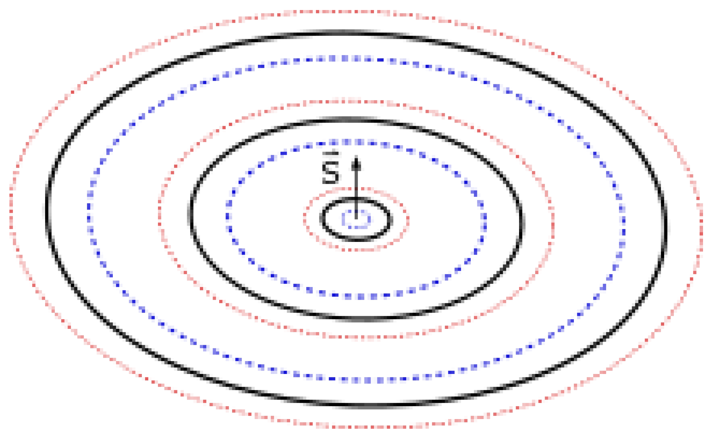
Figure 3.
Strength (intensity) of forces for waveforms of energy.
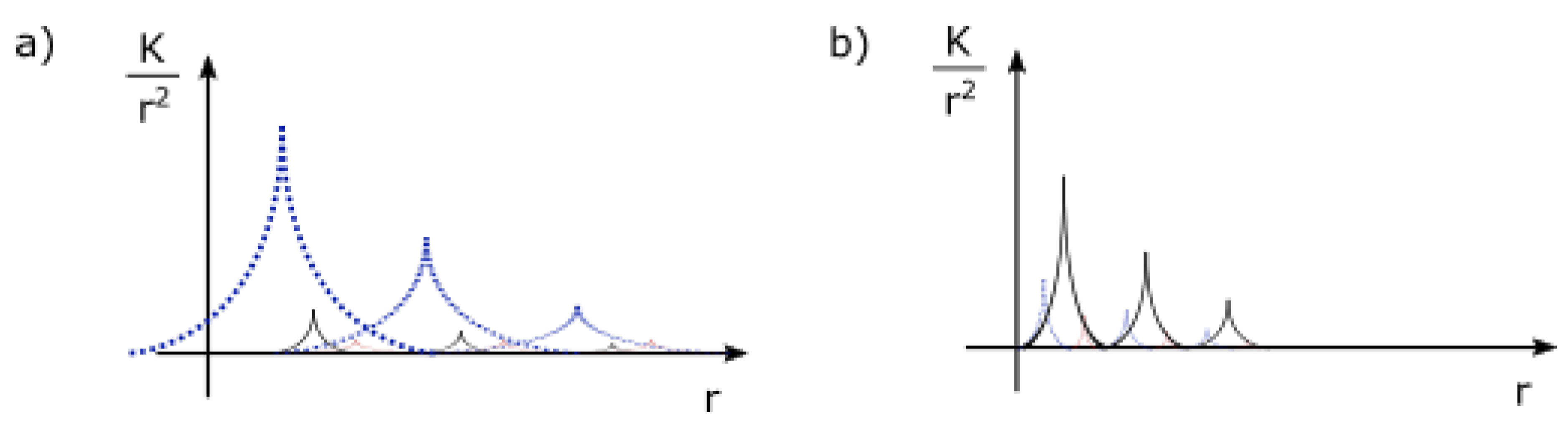
Figure 4.
Primary components of the Solar System, not to scale (planet images source: Pixabay/OpenClipart-Vectors4).
Figure 4.
Primary components of the Solar System, not to scale (planet images source: Pixabay/OpenClipart-Vectors4).
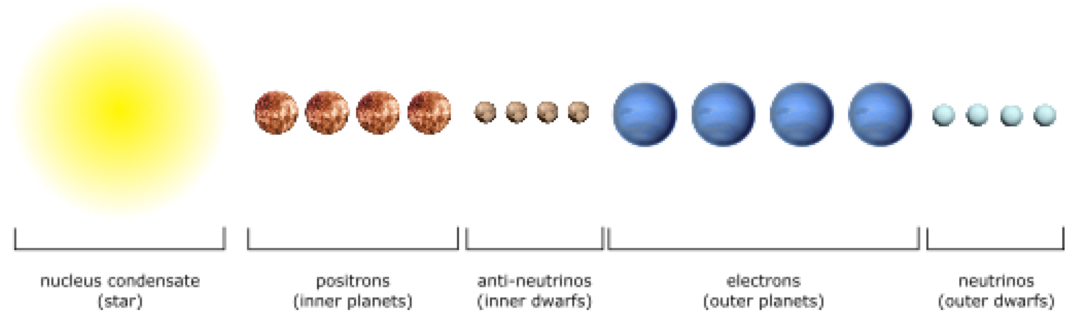
Figure 6.
Primary components of the TOI-178 System, not to scale (planet images source: Pixabay/OpenClipart-Vectors4).
Figure 6.
Primary components of the TOI-178 System, not to scale (planet images source: Pixabay/OpenClipart-Vectors4).
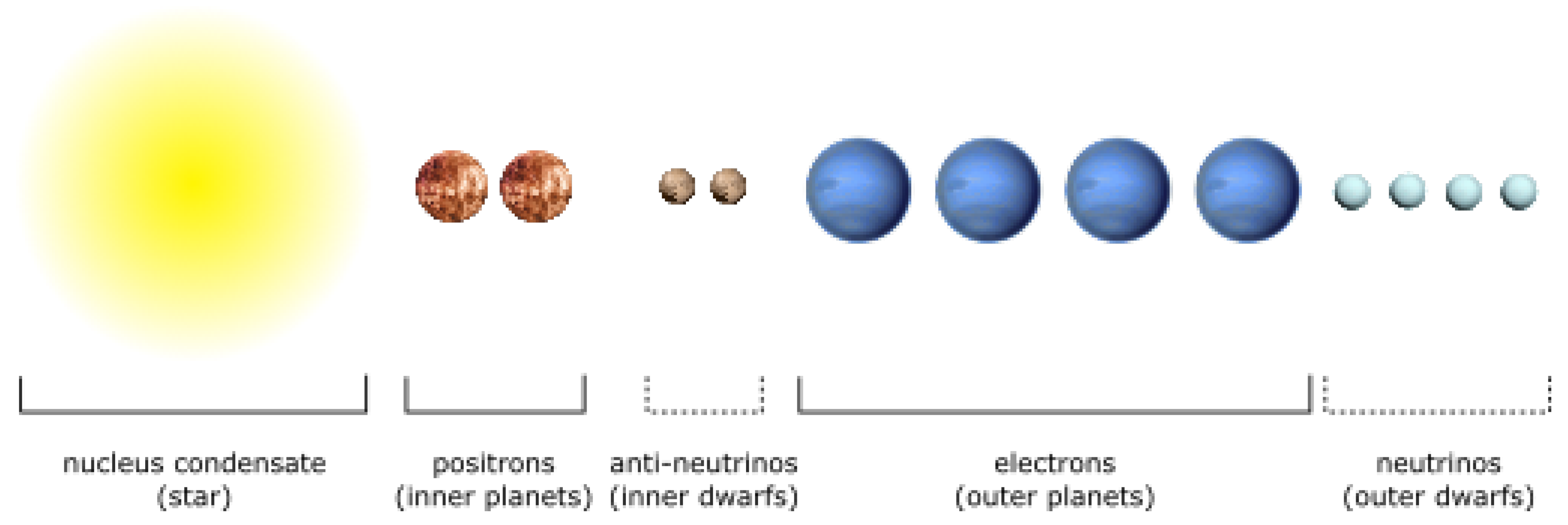
Figure 7.
Masses of detected exoplanets (data source: The Extrasolar Planets ).
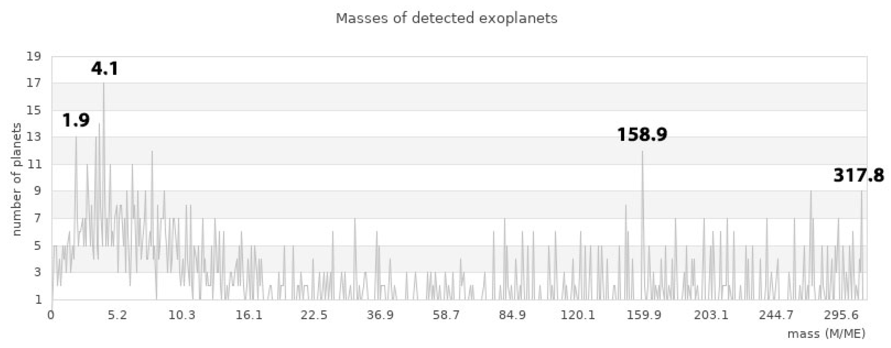
Figure 8.
left) internal rotation of the , right) rotation of spiral .
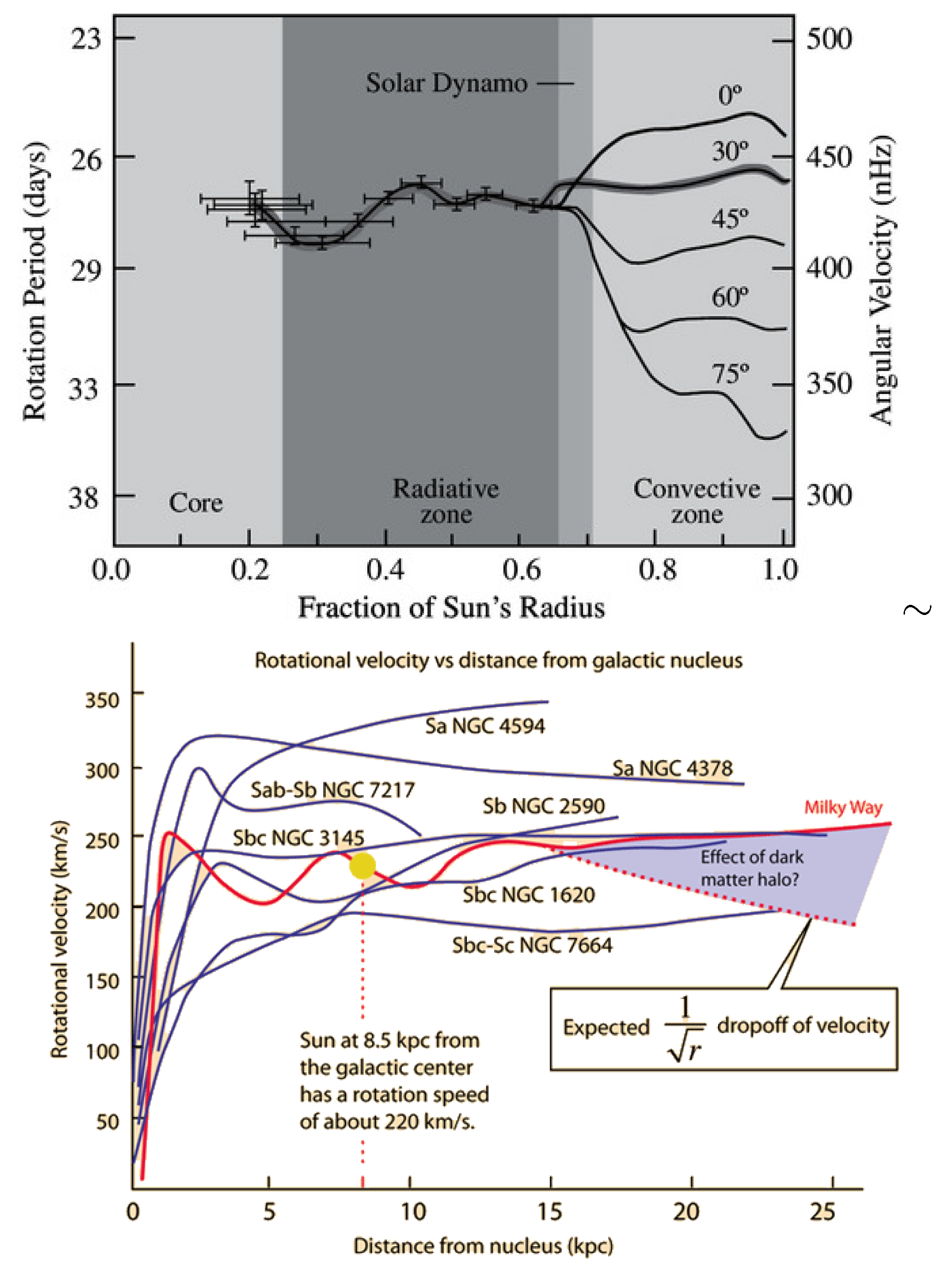
Figure 9.
Rotational velocities of the Sun.
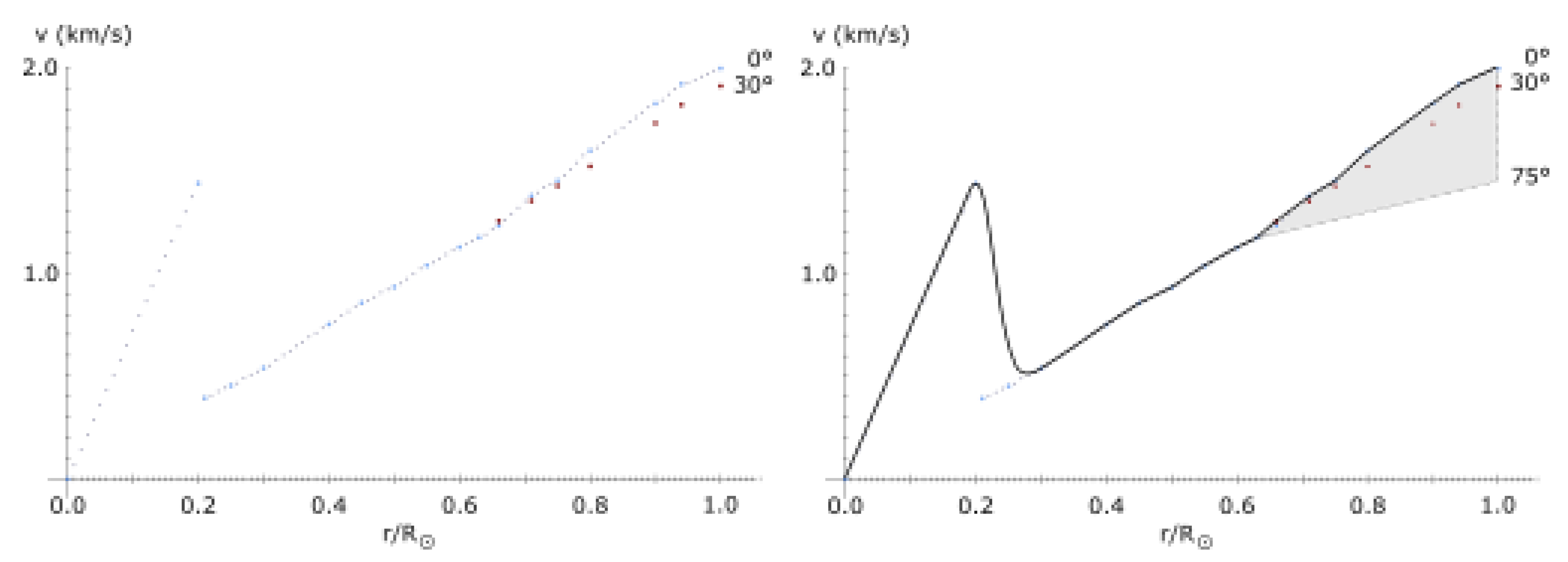
Figure 10.
Rotational velocities of the Sun and near corona.
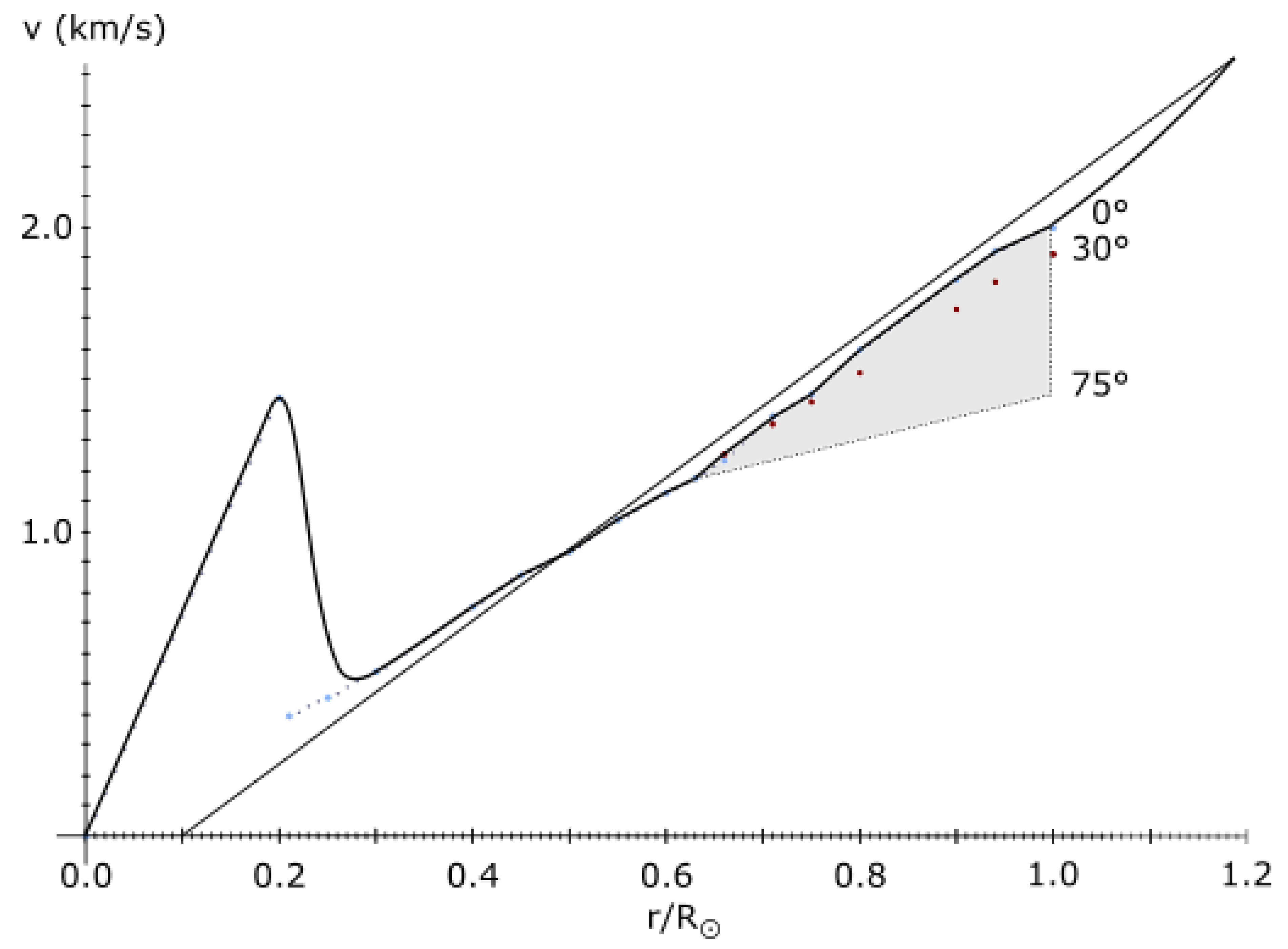
Figure 11.
Oscillation of the gravitational constant.
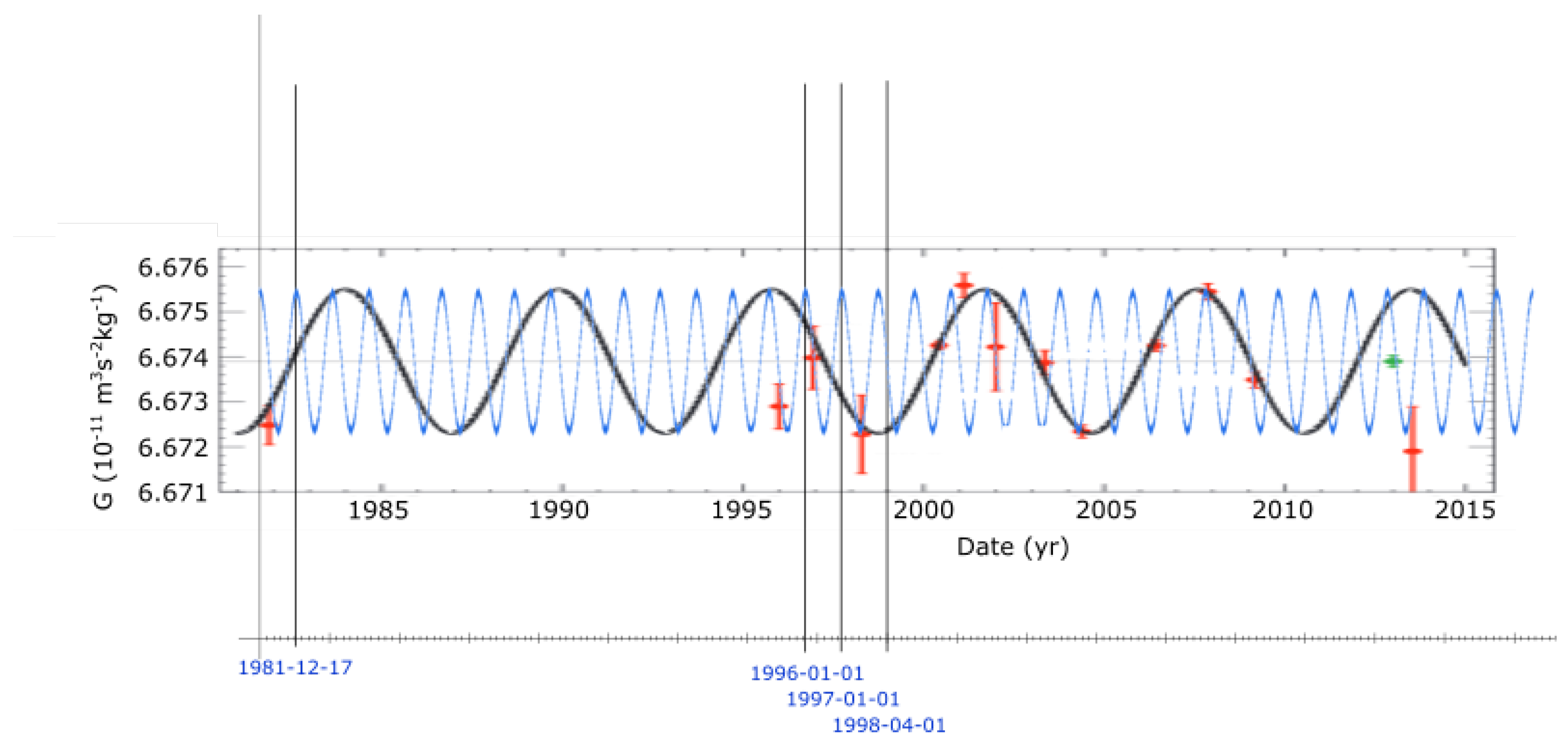
Figure 12.
Oscillation of the gravitational constant.
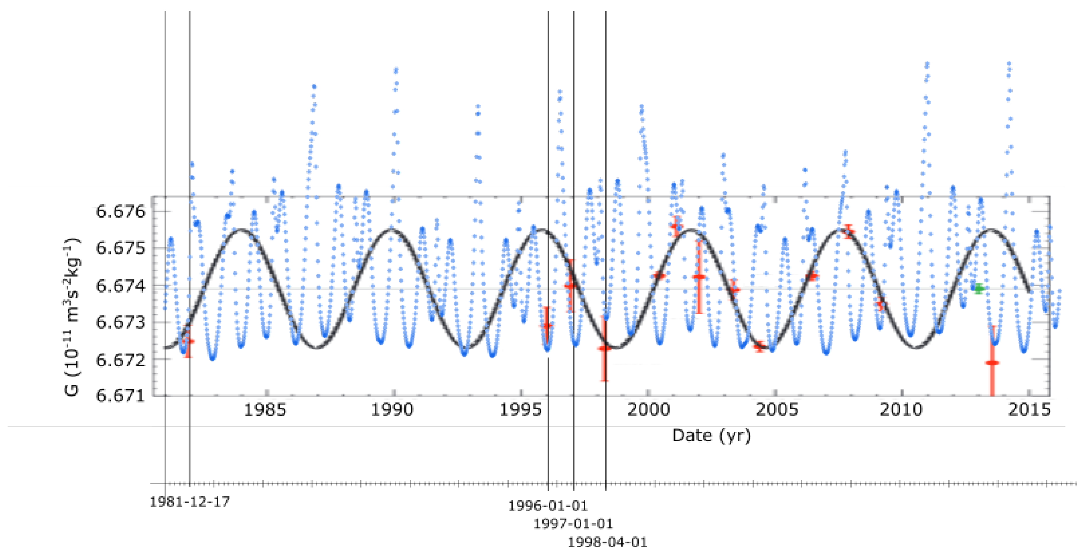
Figure 13.
One interpretation of Sun partitioning in: a) 6p4n state b) 4p6n state (R = radius in 6p4n state)
Figure 13.
One interpretation of Sun partitioning in: a) 6p4n state b) 4p6n state (R = radius in 6p4n state)
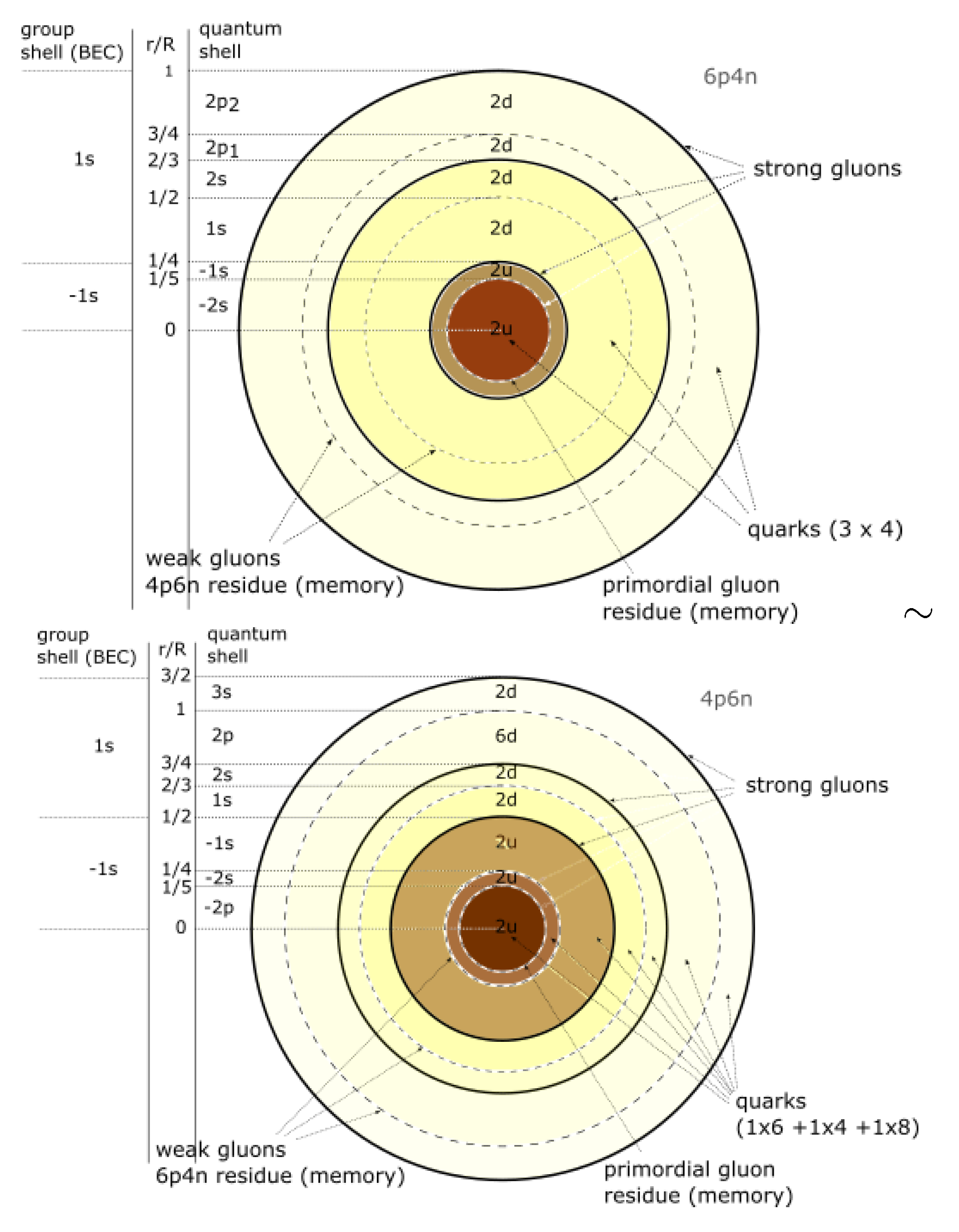
Figure 14.
Equatorial anisotropy of the Earth’s inner .
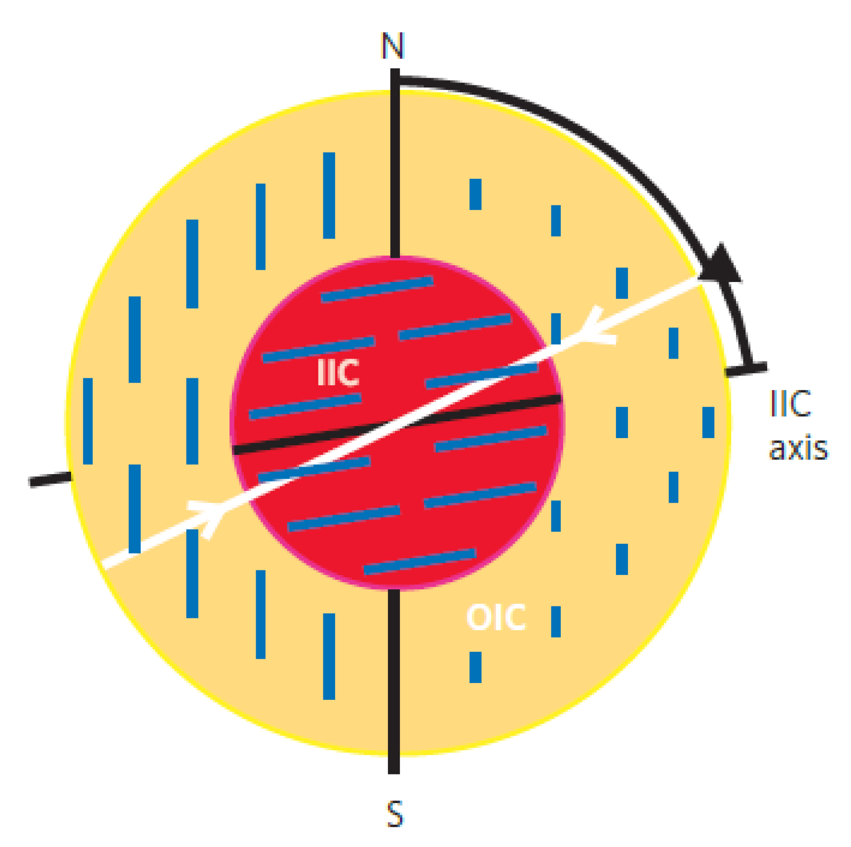
Figure 15.
Magnetic field of , left) , right) (N=2)
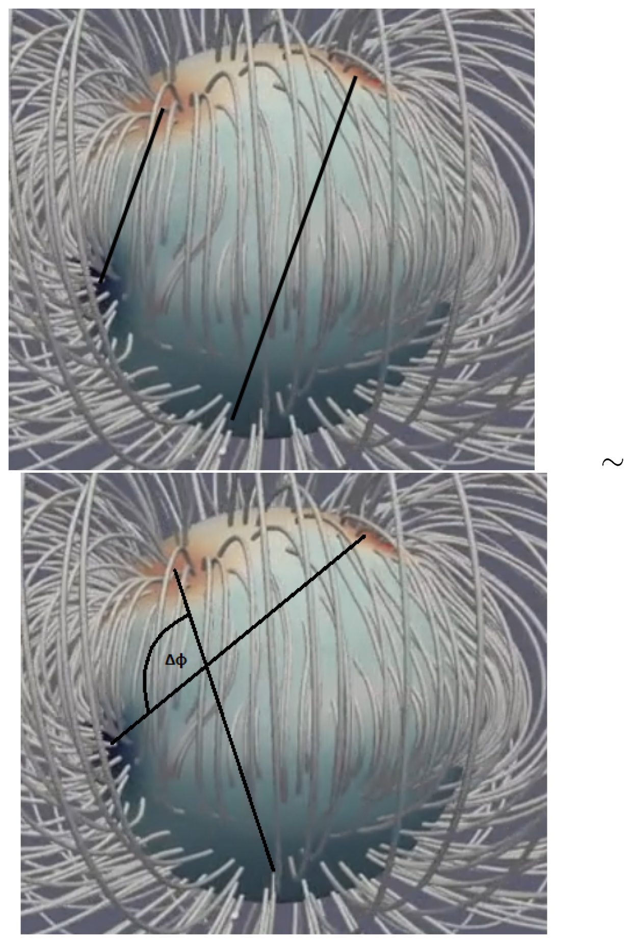
Figure 16.
Uranus’ magnetic field model
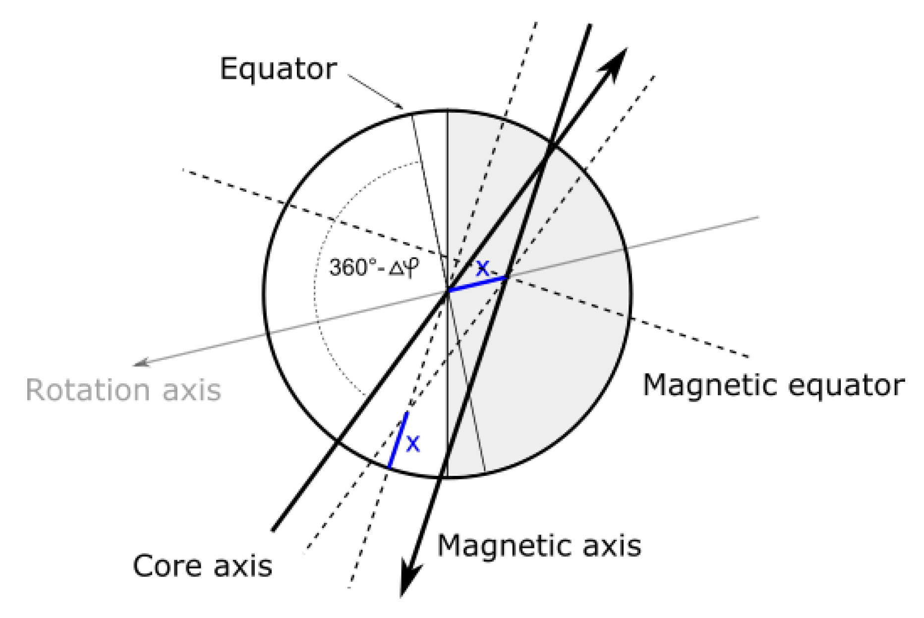
Figure 17.
Neptune’s magnetic field model
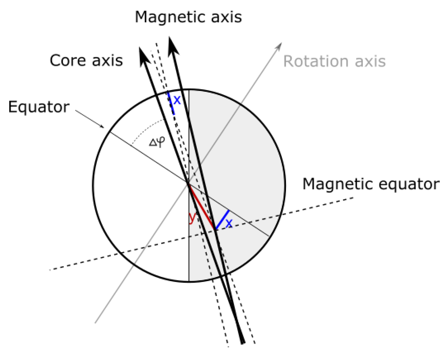
Figure 18.
Layers of Earth’s brain, superimposed on seismic .
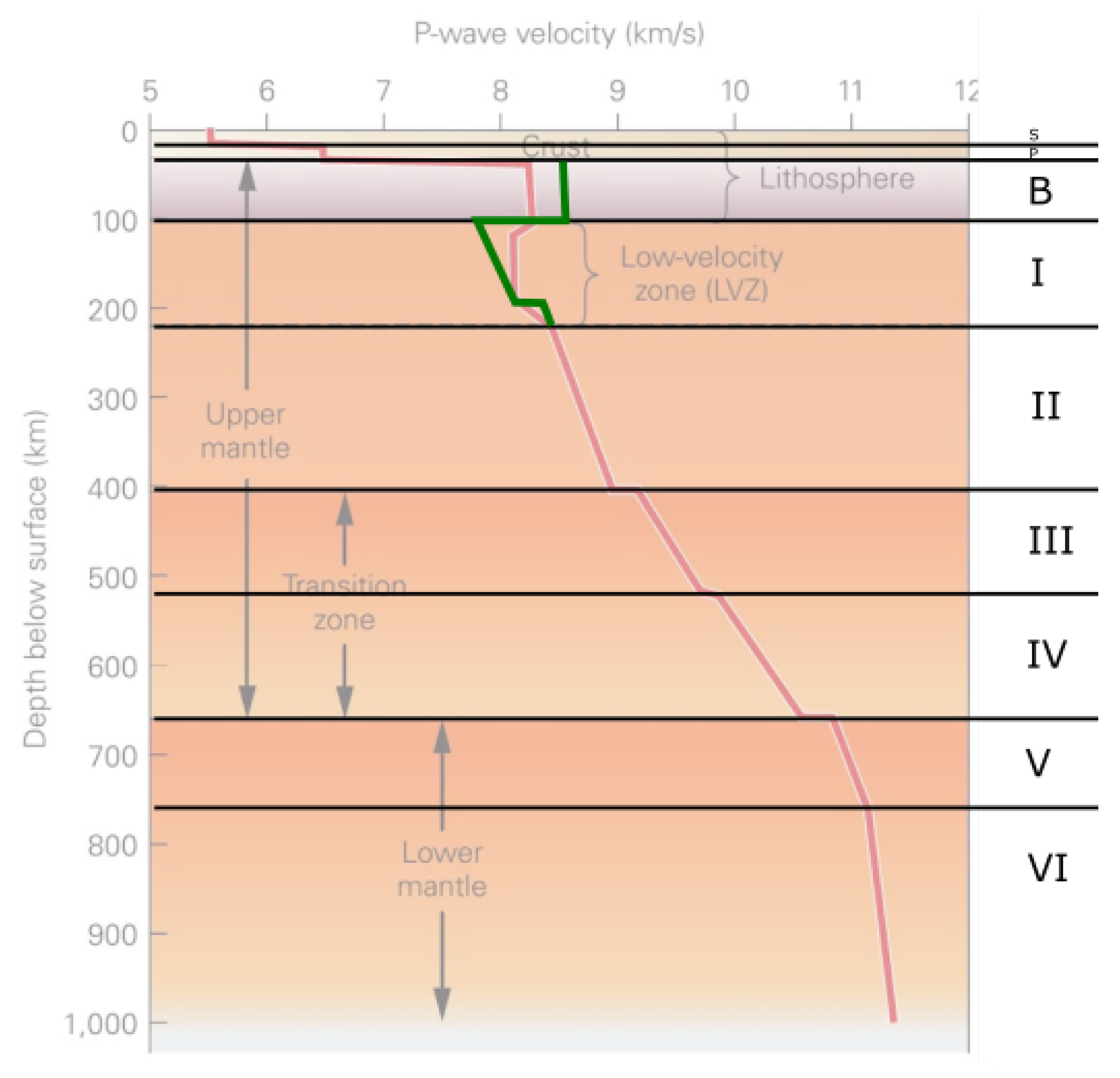
Figure 19.
The history of atmospheric CO2 .
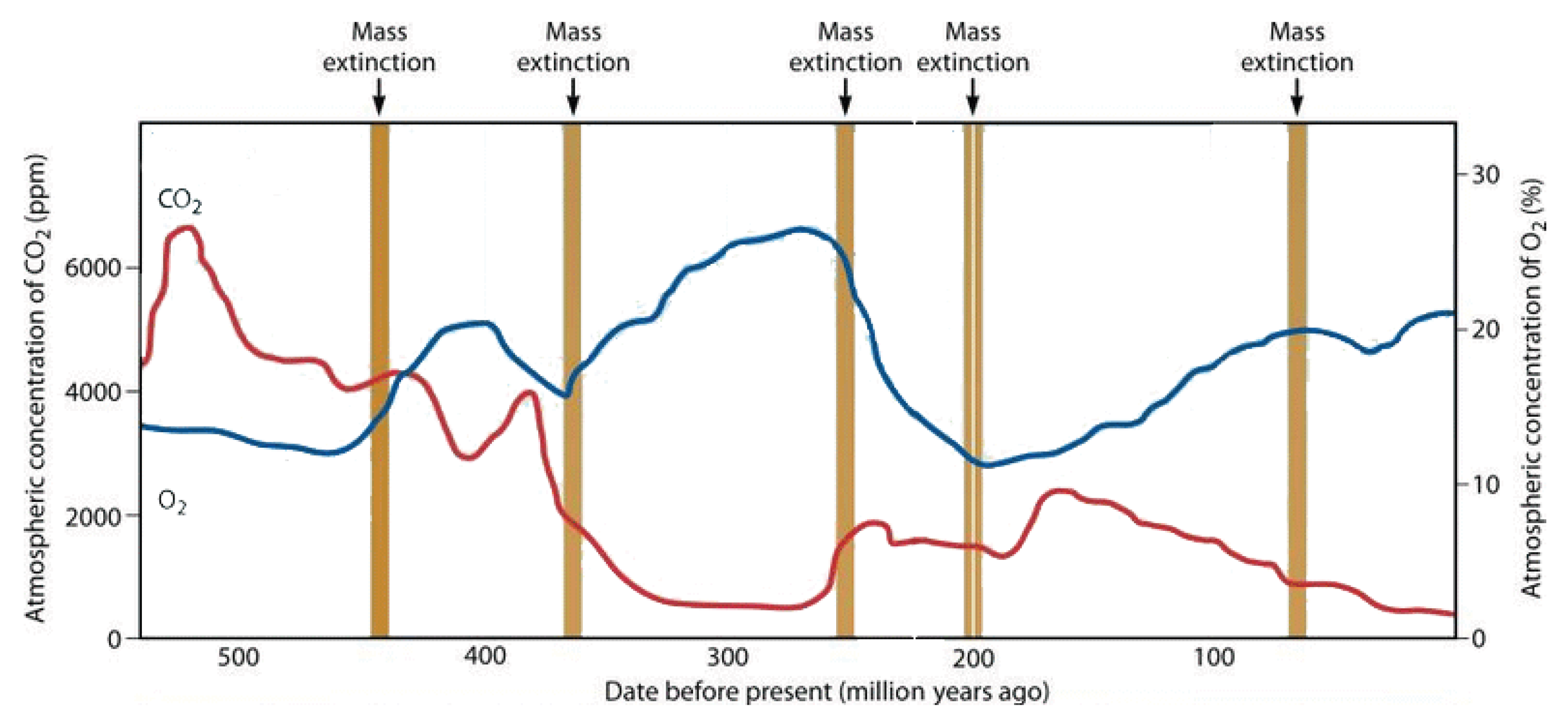
Figure 20.
CO2 pH minimum marker models a) and b) (blue dots = major extinction events, red = minor extinction events, on b) grey = icehouse periods, white = greenhouse periods)
Figure 20.
CO2 pH minimum marker models a) and b) (blue dots = major extinction events, red = minor extinction events, on b) grey = icehouse periods, white = greenhouse periods)
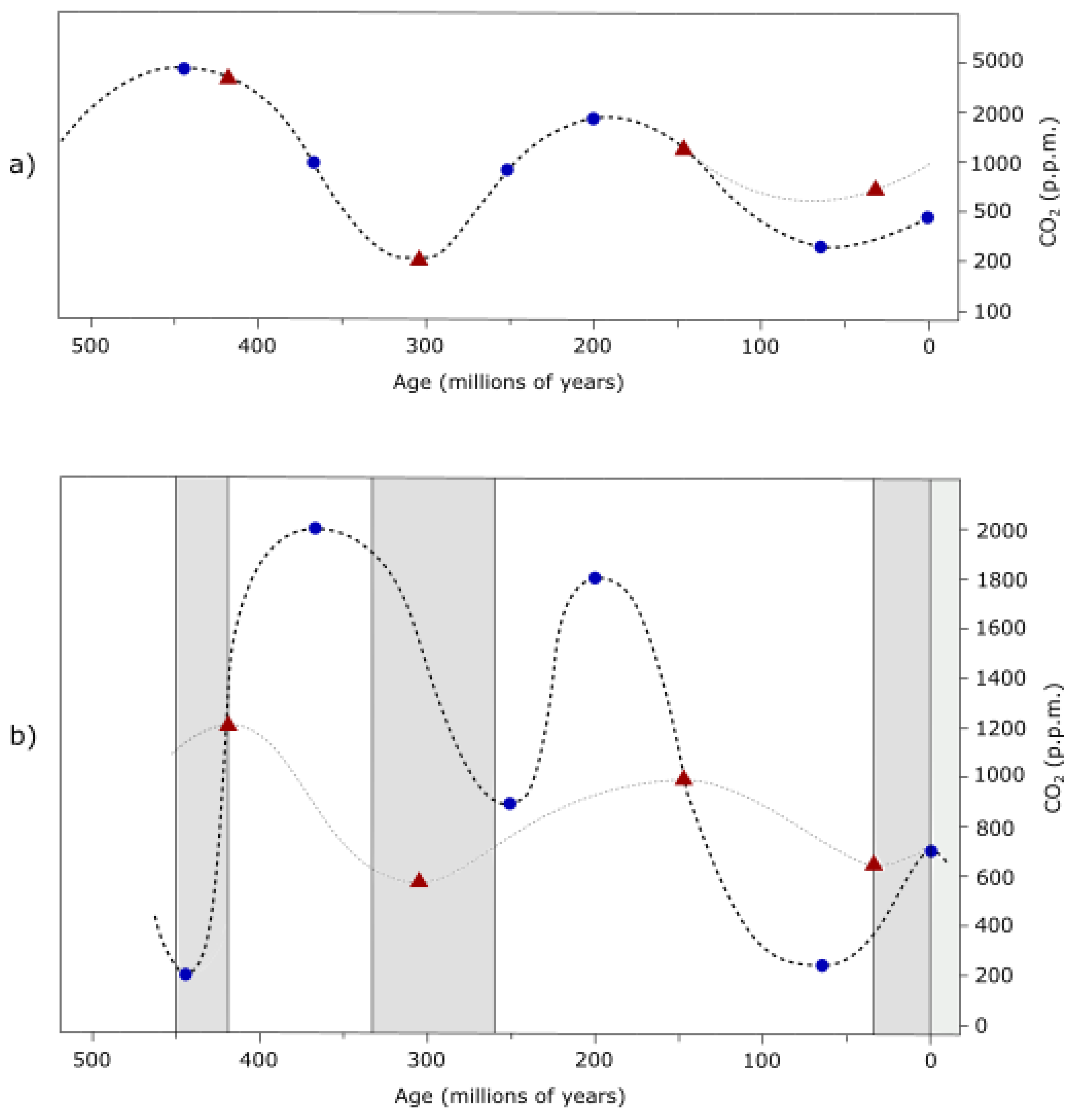
Figure 22.
Neutrino pulse due to decay rate increase.
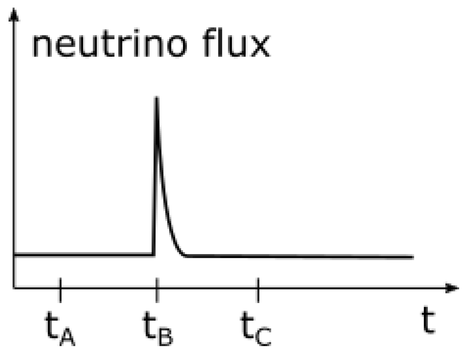
Figure 23.
Dataset 1 - extinctions (left), spectral analysis (right).
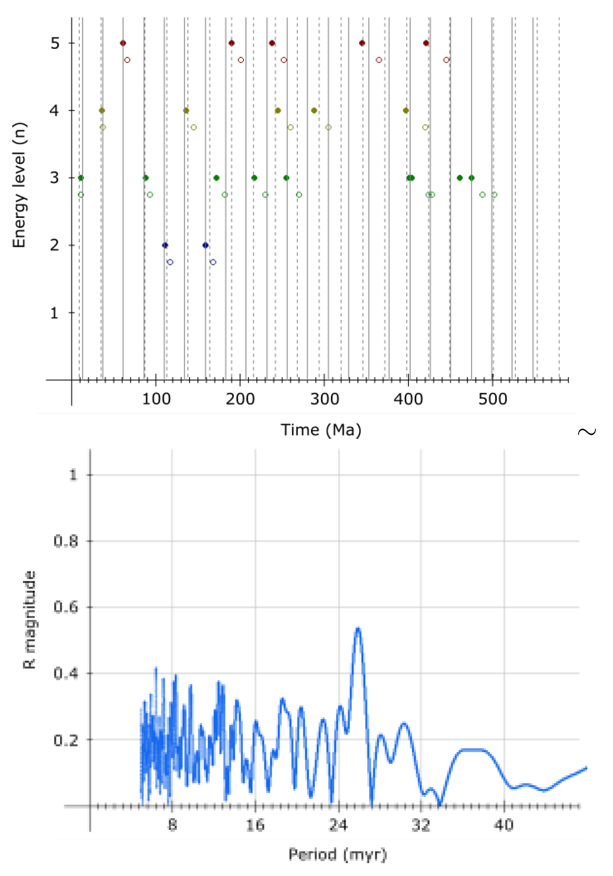
Figure 24.
Dataset 2 - extinctions (left), spectral analysis (right).

Figure 25.
Dataset 3 - extinctions.
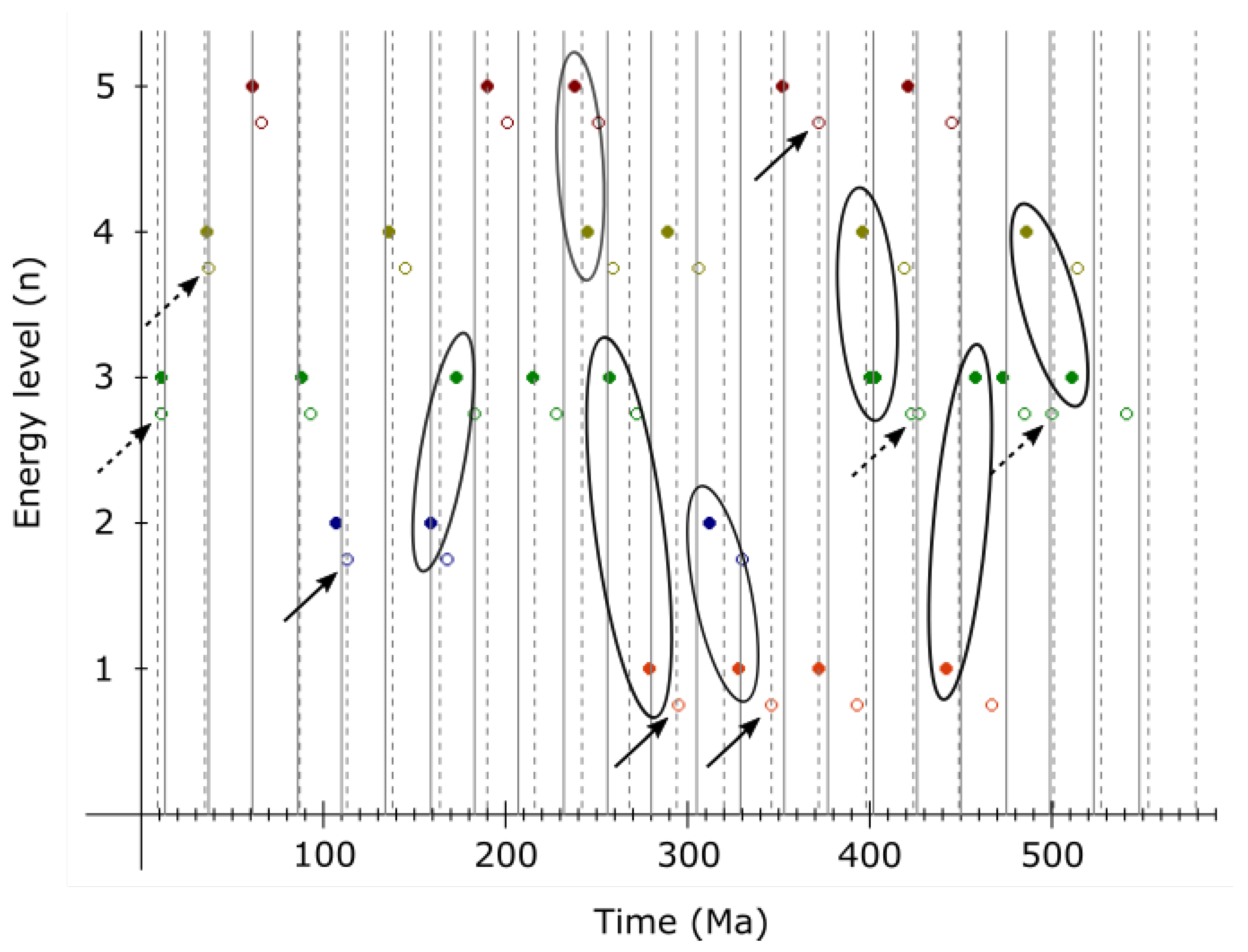
Figure 28.
Correlation of major extinctions (left) with Earth’s mantle layers (right).
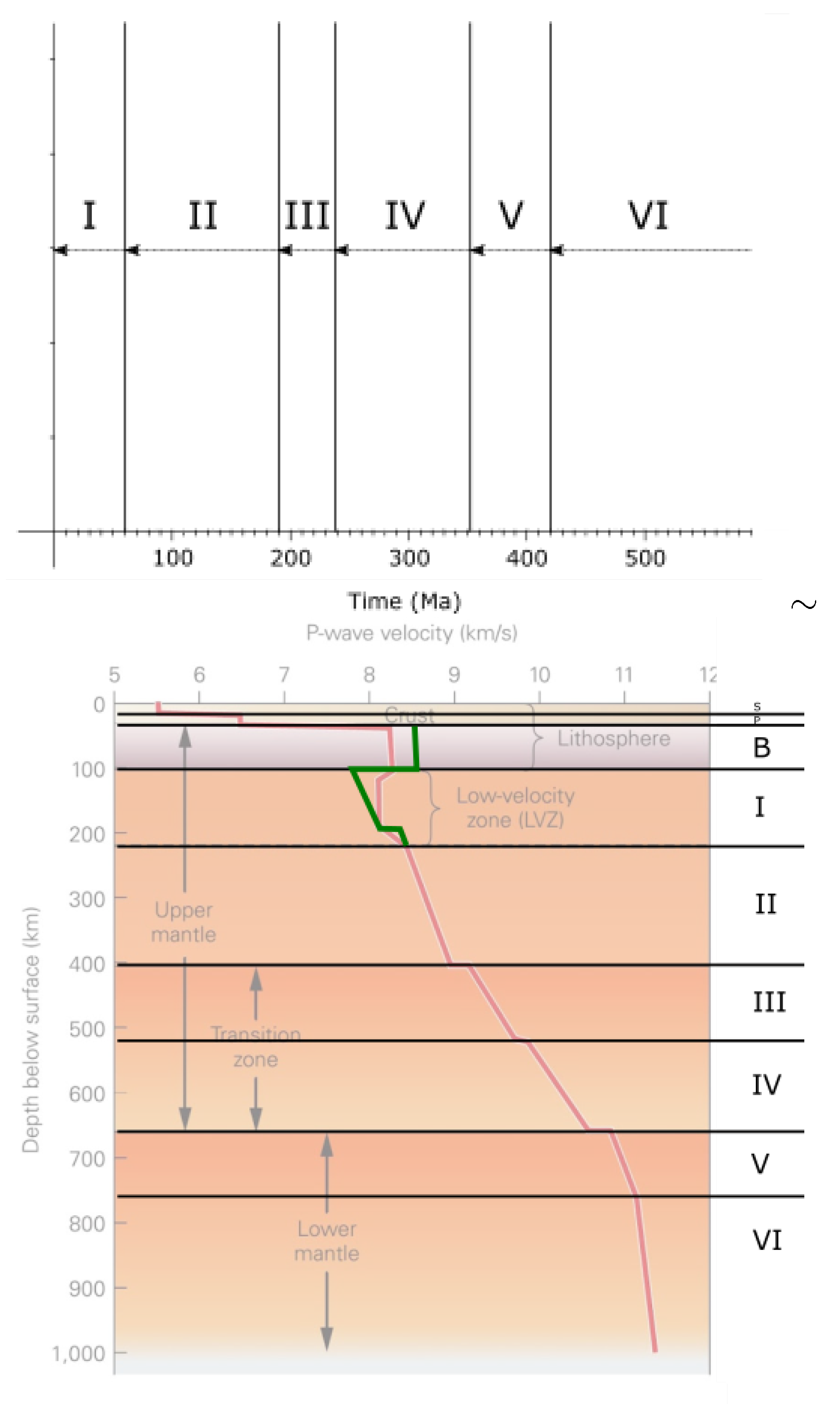
Figure 29.
Homo.beta cell.
Figure 30.
Normal cells.
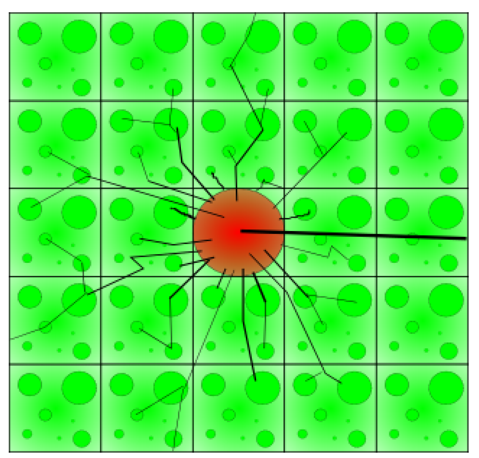
Figure 31.
Rough illustration of Sun’s gravity.
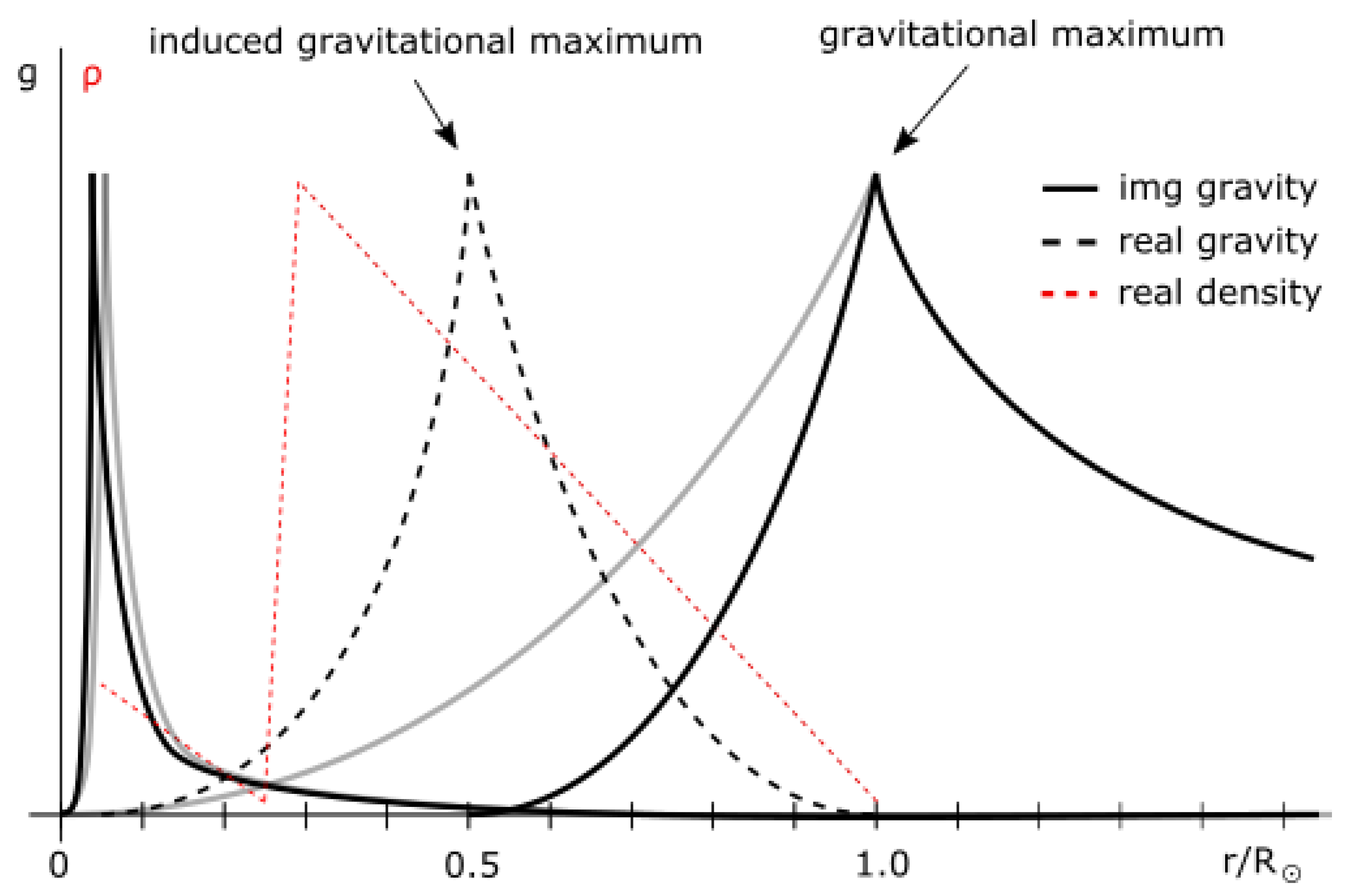
Figure 33.
Stable isotopes of the Solar System in state 6p4n at t > 1495840 years.
Figure 34.
Calculated Hill sphere and measured radius for stable isotopes: a) data from 2008. b) data from 1964.
Figure 34.
Calculated Hill sphere and measured radius for stable isotopes: a) data from 2008. b) data from 1964.
Figure 35.
Calculated Hill sphere (adjusted) and measured radius for stable isotopes: a) data from 2008. b) data from 1964.
Figure 35.
Calculated Hill sphere (adjusted) and measured radius for stable isotopes: a) data from 2008. b) data from 1964.
Figure 36.
Isotopes used in Figure 36 calculation: a) data from 2008. b) data from 1964.
Figure 36.
Isotopes used in Figure 36 calculation: a) data from 2008. b) data from 1964.
Figure 37.
Sun rotation .
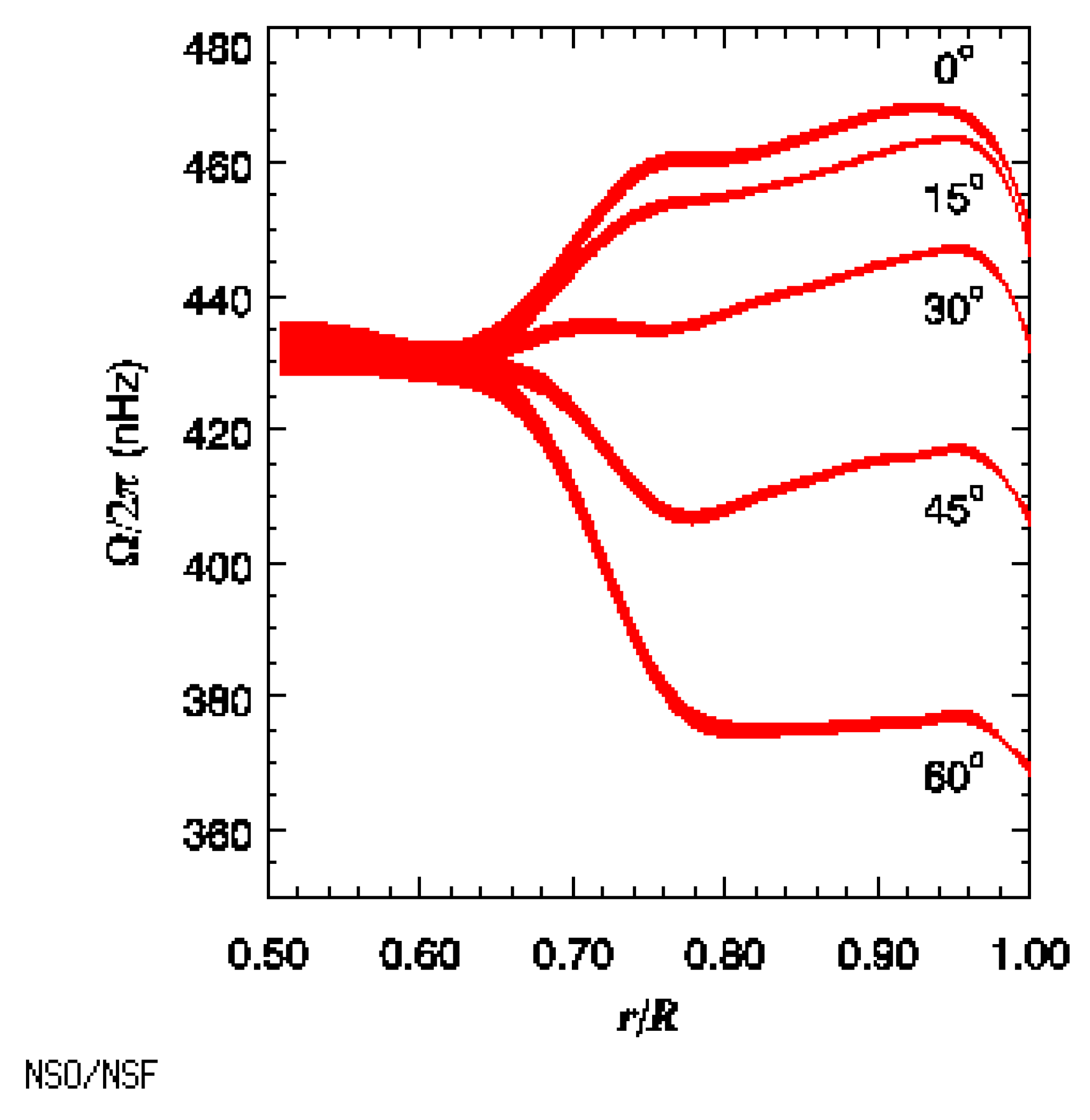
Figure 39.
Mass and charge radii for particles in two different shells.
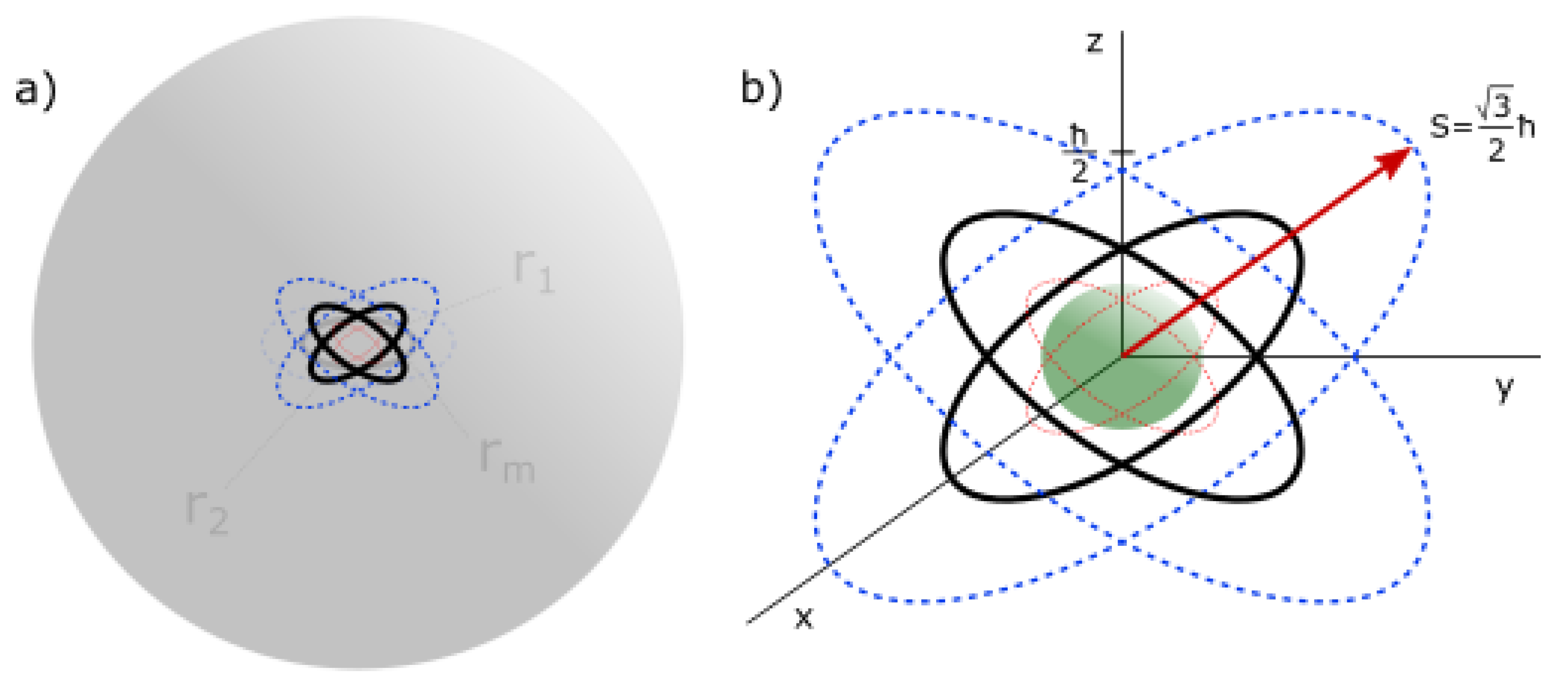
Table 3.
Possible kinetic mass components of outer planets.
| planet | mass ( kg) | 6% of mass, if kept ( kg) | 6% of mass, if lost ( kg) |
|---|---|---|---|
| Jupiter | 1898.190 | 113.8914 | 121.161 |
| Saturn | 568.340 | 34.1004 | 36.277 |
| Uranus | 86.813 | 5.20878 | 5.541 |
| Neptune | 102.413 | 6.14478 | 6.537 |
Table 4.
4th order period correlation with excursions.
| cycle | years before present (calculated) | correlated event |
|---|---|---|
| 0 | ∼0 | current events (extinction, climate change, ozone depletion, likely magnetic excursion or reversal, ...) |
| 1 | 9221.4 | 10Be enrichment in ice cores ≈9200 years ago[79] (hypothesized extreme solar storm event), Lake Michigan/Erie magnetic excursion 10-9 ka and 14-12 ka[80] |
| 2 | 18442.8 | Hilina Pali magnetic excursion 18.5 ka[81] |
| 3 | 27664.2 | Lake Mungo magnetic excursion 30780±520 - 28140±370 and ≈26000 years b.p.[82], Oruanui eruption ≈26.5 ka[83] |
| 4 | 36885.6 | Mono Lake magnetic excursion 36 - 30 ka[84] (34.5 ka[81]), Dome C/Vostok 10 Be enrichment (likely due to excursion) ≈35 ka[85] |
| 5 | 46107.0 | Laschamp magnetic excursion 46.6±2.4 ka[86] (41.2 ka[81]), Neanderthals extinction |
| 6 | 55328.4 | ? |
| 7 | 64549.8 | Norwegian-Greenland Sea magnetic excursion 64.5 ka[81] |
| 8 | 73771.2 | Toba volcanic eruption ≈74000 years ago[87] |
Table 5.
Calculated gravity for outer planets.
| n | planet | orbital velocity v (m/s) | orbital radius r ( km) | total mass M ( kg) | required total mass ( kg) | calc. gravity g () | measured gravity () | measured acc. () | calculated () |
|---|---|---|---|---|---|---|---|---|---|
| 5 | Neptune | 5430 | 4495.06 | 102.413 | 102.413 | 11.15 | 11.15 | 11.00 | 11.00 |
| 5 | Uranus | 6800 | 2872.46 | 86.813 | 127.976 | 8.92 | 8.87 | 8.69 | 8.803 |
| 3 | Saturn | 9680 | 1433.53 | 568.340 | 108.084 | 10.565 | 10.44 | 8.96 | 10.423 |
| 1 | Jupiter | 13060 | 778.57 | 1898.190 | 49.168 | 23.225 | 24.79 | 23.12 | 22.912 |
Table 6.
Calculated gravity for inner planets.
| n | planet (mirror) | orbital velocity v (m/s) | orbital radius r ( km) | total mass ( kg) | required total mass ( kg) | calc. gravity g () | gravity () |
|---|---|---|---|---|---|---|---|
| 5 | Mercury (Neptune) | 47360 | 57.91 | 0.330 | 0.33011 | 3.70 | 3.70 |
| 3 | Venus (Uranus) | 35020 | 108.21 | 4.868 | 0.14335 | 8.52 | 8.87 |
| 3 | Earth (Saturn) | 29780 | 149.6 | 5.972 | 0.12193 | 10.02 | 9.798 |
| 10 | Mars (Jupiter) | 24070 | 227.92 | 0.642 | 0.33006 | 3.70 | 3.71 |
Table 7.
Obtained ℏ for outer planets, including other properties.
| n | l | s | planet | orbital vel. (m/s) | orbital radius ( km) | used spin vel. (m/s) | obtained localized spin radius (km) | spin rot. period (h) | calc. ℏ (Js) |
|---|---|---|---|---|---|---|---|---|---|
| 4 | 3 | 0 | Neptune | 5430 | 4495.06 | +12293 | 113468 | 16.11 | 1.6098 × |
| 3 | 2 | 0 | Uranus | 6800 | 2872.46 | +12293 | 121427 | 17.24 | 1.5673 × |
| 2 | 1 | 0 | Saturn | 9680 | 1433.53 | +12293 | 75054 | 10.656 | 1.5591 × |
| 1 | 0 | +1/2 | Jupiter | 13060 | 778.57 | +12293 | 69911 | 9.9250 | 1.5955 × |
Table 9.
Obtained ℏ for outer planets, respecting dipole tilt, including other properties.
| n | l | s | planet | orbital vel. (m/s) | orbital radius ( km) | spin vel. (m/s) | spin radius (km) | spin rot. period (h) | calc. ℏ (Js) | |
|---|---|---|---|---|---|---|---|---|---|---|
| 5 | - 46.[129] = +43. | 1/2 | +1/2 | Neptune | 5430 | 4495.06 | +2668 | 24622 | 16.11 | 1.362 × |
| 5 | + 58.[130] = -31. | 3 +1/2 | -4 -1/2 | Uranus | 6800 | 2872.46 | -2568 | 25362 | 17.24 | 1.3669 × |
| 3 | [131] | 1 | 0 | Saturn | 9680 | 1433.53 | +9538 | 58232 | 10.656 | 1.3636 × |
| 1 | +9.[132] | 0 | +1 | Jupiter | 13060 | 778.57 | +12293 | 69911 | 9.9250 | 1.3632 × |
Table 10.
Obtained ℏ for outer planets in alternative states, including other properties.
| n | l | s | planet | orbital vel. (m/s) | orbital radius ( km) | spin vel. (m/s) | spin radius (km) | spin rot. period (h) | calc. ℏ (Js) |
|---|---|---|---|---|---|---|---|---|---|
| 3 | 1 | 1/2 | Neptune | 5430 | 4495.06 | 2668 | 24622 | 16.11 | 1.3310 × |
| 3 | 1 | 0 | Uranus | 6800 | 2872.46 | 2568 | 25362 | 17.24 | 1.3319 × |
| 2 | 1 | 0 | Saturn | 9680 | 1433.53 | 9538 | 58232 | 10.656 | 1.3636 × |
| 1 | 0 | 1 | Jupiter | 13060 | 778.57 | 12293 | 69911 | 9.9250 | 1.3817 × |
Table 11.
Possible parameters for inner planets, including other properties.
| l | s | planet | total mass ( kg) | orbital vel. (m/s) | orbital radius ( km) | spin vel. (m/s) | spin radius (m) | calc. ℏ (Js) | |
|---|---|---|---|---|---|---|---|---|---|
| 0 | 1 | Mars | 0.642 | 24070 | 227.92 | 61401 | ? | 1.3636 × | |
| +9.[134] | 1 | 0 | Earth | 5.972 | 29780 | 149.6 | 156855 | ? | 1.3636 × |
| 1 | -1 | Venus | 4.868 | 35020 | 108.21 | 39549 | ? | 1.3636 × | |
| [135] | 1/2 | -1 | Mercury | 0.330 | 47360 | 57.91 | -2292 | ? | 1.3636 × |
Table 12.
Calculated spin radius for inner planets.
| planet | total mass M ( kg) | orbital radius ( km) | spin radius (m) |
|---|---|---|---|
| Mars | 0.642 | 227.92 | 24851090 |
| Earth | 5.972 | 149.6 | 1753428 |
| Venus | 4.868 | 108.21 | 1556019 |
| Mercury | 0.330 | 57.91 | 12283939 |
Table 14.
Standard particle candidates for planets, with listed electric charges.
| planet | configuration | particle species (charge) | total charge |
|---|---|---|---|
| Mercury | 1e | positron () | |
| Venus | 1e | anti-down quark (1/) | 1/ |
| Earth | 2e | anti-down quark (1/) | 2/ |
| Mars | 2e | positron () | |
| Jupiter | 2e | anti-charm quark (2/) | 4/ |
| Saturn | 2e | meson () | |
| Uranus | 1e | strange quark (1/) | 1/ |
| Neptune | 1e | strange quark (1/) | 1/ |
Table 15.
Standard particle candidates for planets.
| planet | mass M [ kg] | particle candidates () | alternative () |
|---|---|---|---|
| Mercury | 0.330 | 1 x positron (0.511) | 1 x positron (0.511) |
| Venus | 4.868 (4.592*) | 1 x anti-down quark (≈4.6) | 1 x anti-down quark (≈4.8 or 4.6) |
| Earth | 5.972 (5.634*) | 1 x anti-down quark (≈4.6) + 1 x positron (0.511), or 2 x up quark (2 x 2.7475) | 1 x anti-down quark (≈4.8 or 4.6) + 2 x positron (2 x 0.511), or 2 x up quark (2 x 2.07) + 1 x positron (0.511) |
| Mars | 0.642 | 1 x positron (0.511) | 1 x positron (0.511) |
| Jupiter | 1898.19 (1777*) | 1 x tau electron (1776.86) | 1 x tau electron (1776.86) |
| Saturn | 568.32 (532.06*) | 1 x muon anti-up quark (568.32**) | 1 x muon anti-up quark (428***) + 1 x muon electron (105.658) |
| Uranus | 86.813 | 1 x muon electron (105.658) | 1 x muon electron (105.658) |
| Neptune | 102.413 (96.876*) | 1 x muon electron (105.658) | 1 x muon electron (105.658) |
Table 16.
Sums of charges
| configuration | charge sum [e] |
|---|---|
| 1 x positron, 1 x anti-down quark, 1 x anti-down quark + 1 x positron, 1 x positron | + (3+2/3) |
| 1 x tau e, 1 x muon anti-up quark, 1 x muon e, 1 x muon e | - (3+2/3) |
Table 17.
Sums of charges.
| configuration | charge sum [e] |
|---|---|
| 1 x positron, 1 x anti-down quark, 1 x anti-down quark + 2 x positron, 1 x positron | + (4+2/3) |
| 1 x tau e, 1 x muon anti-up quark + 1 x muon e, 1 x muon e, 1 x muon e | - (4+2/3) |
Table 18.
U1 masses of terrestrial planets.
| planet | ( kg) | m (kg) |
|---|---|---|
| Mercury | 0.330 | 3.84 × |
| Venus | 4.868 | 5.67 × |
| Earth | 5.972 | 6.95 × |
| Mars | 0.642 | 7.48 × |
Table 19.
Calculated neutral and current radii, compared to measured R.
| N | n | planet | M (kg) | r ( km) | s | p | (∘) | neutral R (km) | current R (km) | R (km) |
|---|---|---|---|---|---|---|---|---|---|---|
| 2 | 5 | Neptune | 1.02413 × | 4495.06 | 1 | 2 | 36.7084 | 24764 | 24764 | 24764 |
| 2 | 5 | Uranus | 8.6813 × | 2872.46 | 1 | 1 | 233.1511 | 25703 | 25559 | 25559 |
| 2 | 3 | Saturn | 5.6834 × | 1433.53 | 2 | 1 | 0.2 | 60806 | 60268 | 60268 |
| 1 | 1 | Jupiter | 1.89819 × | 778.57 | 2 | 1 | -0.847 | 68848 | 71492 | 71492 |
| 2 | 5 | Mercury | 3.3011 × | 57.91 | 2 | 2 | 172.3047 | 2555.7 | 2439.7 | 2439.7 |
| 2 | 3 | Venus | 4.8675 × | 108.21 | 1 | 0 | 0 | 6051.8 | 6051.8 | 6051.8 |
| 2 | 3 | Earth | 5.9723 × | 149.60 | 2 | 1 | 90.3135 | 6284.72 | 6378.14 | 6378.14 |
| 1 | 10 | Mars | 6.4171 × | 227.92 | 1 | 2 | -91.9957 | 3394.1 | 3396.2 | 3396.2 |
Table 20.
Correlation of outer and inner planets, in case of anti-aligned and aligned entanglements.
Table 20.
Correlation of outer and inner planets, in case of anti-aligned and aligned entanglements.
| planet | normalized (∘) | entanglement (anti-aligned) | entanglement (aligned) |
|---|---|---|---|
| Neptune | (5 × 36) % 360 = 180 | Venus | Mercury |
| Uranus | (5 × 234) % 360 = 90 | Mars | Earth |
| Saturn | (5 × 0) % 360 = 0 | Mercury | Venus |
| Jupiter | (5 × 0) % 360 = 0 | Mercury | Venus |
Table 21.
One interpretation/state of Earth’s gravity.
| n | correlated discontinuity | radius (m) | gravity () |
|---|---|---|---|
| 1 | thermopause | 6822815 | 8.56 (274 / ) |
| 1 | crust surface | 6371000 | 9.82 |
| 1 | crust surface perihelion | 6357000 | 9.86 |
| 1 | real surface | 6307105 | 10.02 |
| 1 | outer core / mantle | 3411408 | 34.25 (274 / ) |
| 1 | transition zone (induced charge radius) | 1705704 | 137 (274 / 2) |
| 1 | g. maximum = inner core radius = | 1206115 | 274 |
| 1 | transition zone | 852852 | 137 |
| 1 | inner inner core | 603058 | 69 (274 for n=2) |
Table 22.
Orbital velocities of time and event horizon dimensions.
| n | Planet | i | j | (km/s) | km/s (entanglement) | (current value) | (entanglement) km/s | (neutron correction) | (entanglement) km/s |
|---|---|---|---|---|---|---|---|---|---|
| 4 | Mercury | 2 | -1 | 47.36 | 5.47 (Neptune) | × = -0.04 | 12.033 (Jupiter) | +4.73 | 16.77 (Hygiea) |
| 3 | Venus | 1 | 0 | 35.02 | 6.78 (Uranus) | × = +0.02 | 16.63 (Hygiea) | +1.275 | 17.9 (Ceres) |
| 2 | Earth | 0 | 1 | 29.78 | 9.66 (Saturn) | × = +0.02 | 19.55 (Vesta) | -1.66 | 17.88 (Pallas) |
| 1 | Mars | -1 | 2 | 24.07 | 13.08 (Jupiter) | × = -0.02 | 24.07 (Mars) | -4.73 | 19.34 (Vesta) |
Table 24.
CO2 pH minimum marker models.
| year [mya] | a) [ppm] | b) [ppm] | c) [ppm] | d) [ppm] | e) [ppm] |
|---|---|---|---|---|---|
| 444 | 3800 | 200 | 2000 | 3800 | 2000 |
| 370 | 1000 | 2000 | 1000 | 1800 | 1200 |
| 252 | 800 | 900 | 800 | 800 | 800 |
| 201 | 1800 | 1800 | 1800 | 1800 | 600 |
| 66 | 250 | 250 | 250 | 300 | 500 |
| 0 | 450 | 700 | 750 | 800 | 450 |
Table 25.
Some calculated impact dates, correlated with potential impactors.
| [ppm] | year of impact | associated impactor (diameter) | impactor closest approaches | additional candidates (diameter) |
|---|---|---|---|---|
| 450 | 2029 | 99942 Apophis (≈375 m[226]) | 2029, 2051, 2066[227] | (≈37 m) |
| 500 | 2040 | 6037 (1988 EG) (≈400 m[228]) | 2041[229] | |
| 700 | 2066 | 99942 Apophis (≈375 m) | 2029, 2051, 2066 | |
| 750 | 2071 | 1866 Sisyphus (≈7 km[230]) | 2058, 2071[231] | (≈37 m) |
| 800 | 2075 | 162173 Ryugu (≈1 km[232]) | 2076[233] |
Table 26.
Calculation and of 10Be half-life.
| year | calculated [ years] | sample | measured [ years] |
|---|---|---|---|
| 1947 | 1.665 | 1.7 ±0.4 * † | |
| 1947 (2) | 1.665 | 1.6 ±0.2 * † | |
| 1972 | 1.608 | 1.5 ±0.3 | |
| 1975 | 1.597 | 1.48 ±0.15 | |
| 1986 | 1.550 | NIST-4325 | 1.34 ±0.07 |
| 1987 | 1.545 | ORNL-MASTER | 1.51 ±0.06 † |
| 1993 | 1.513 | NIST-4325 | 1.53 ±5% (1.53 ±0.07) † |
| 1993 (2) | 1.513 | ICN | 1.48 ±5% (1.48 ±0.06) † |
| 2007 | 1.413 | ICN | 1.36 ±0.07 |
| 2010 | 1.387 | 1.388 ±0.018 | |
| 2010 (2) | 1.387 | 1.386 ±0.016 |
Table 27.
Calculation and measurements of 10Be half-life.
| year | calculated [ years] | sample | measured [ years] |
|---|---|---|---|
| 1947 | 1.676 ±0.044 | 1.7 ±0.4 * † | |
| 1947 (2) | 1.676 ±0.044 | 1.6 ±0.2 * † | |
| 1972 | 1.593 ±0.044 | 1.5 ±0.3 | |
| 1975 | 1.579 ±0.044 | 1.48 ±0.15 | |
| 1986 | 1.518 ±0.044 | NIST-4325 | 1.34 ±0.07 |
| 1987 | 1.512 ±0.044 | ORNL-MASTER | 1.51 ±0.06 † |
| 1993 | 1.473 ±0.044 | NIST-4325 | 1.53 ±5% (1.53 ±0.07) † |
| 1993 (2) | 1.473 ±0.044 | ICN | 1.48 ±5% (1.48 ±0.06) † |
| 2007 | 1.365 ±0.044 | ICN | 1.36 ±0.07 |
| 2010 | 1.339 ±0.044 | 1.388 ±0.018 | |
| 2010 (2) | 1.339 ±0.044 | 1.386 ±0.016 |
Table 28.
Extinction events dataset 1, sources: , , , , , , , ,
| energy level | extinction events [mya] | extinction events (), age corrected [mya] |
|---|---|---|
| 5 | 66*, 201.3*, 252.2*, 365, 445 | 61.986, 190.208, 238.316, 345.385, 421.148 |
| 4 | 37.8*, 145*, , , | 36.206, 136.774, 245.993, 288.3, 397.519 |
| 3 | 11.6*, 93.9*, 182.7*, , 270, 424e, , , 502 | 11.402, 88.465, 172.88, 217.463, 255.844, 401.469, 404.42, 461.48, 475.257 |
| 2 | , 168.3* | 111.194, 159.702 |
Table 34.
Comparison of weak evolution periods and mantle layers, sources: , , , .
| i | Period of weak evolution T [My] | Normalized period of weak evolution | Corresponding mantle layer thickness D [km] | Normalized layer thickness |
|---|---|---|---|---|
| 5 | 421.348 - 352.461 = 68.887 | 0.163 | - = 120 | 0.176 |
| 4 | 352.461 - 238.041 = 114.42 | 0.272 | - = 140 | 0.206 |
| 3 | 238.041 - 190.308 = 47.733 | 0.113 | - = 110 | 0.162 |
| 2 | 190.308 - 61.986 = 128.322 | 0.305 | - = 190 | 0.279 |
| 1 | 61.986 - 0 = 61.986 | 0.147 | - = 120 | 0.176 |
Table 35.
Correlation of weak evolution periods and mantle layers (or, major extinctions and discontinuities).
Table 35.
Correlation of weak evolution periods and mantle layers (or, major extinctions and discontinuities).
| i | Period of weak evolution T [My] | Normalized period of weak evolution | Corresponding mantle layer thickness D [km] | Normalized layer thickness |
|---|---|---|---|---|
| 5 | 421.3 - 352.5 = 68.8 | 0.163 | 780 - 670 = 110 | 0.162 |
| 4 | 352.5 - 245.8 = 106.7 | 0.253 | 670 - 500 = 170 | 0.250 |
| 3 | 245.8 - 190.3 = 55.5 | 0.132 | 500 - 410 = 90 | 0.132 |
| 2 | 190.3 - 62.0 = 128.3 | 0.305 | 410 - 200 = 210 | 0.309 |
| 1 | 62.0 - 0 = 62.0 | 0.147 | 200 - 100 = 100 | 0.147 |
Table 36.
Correlation of weak evolution periods and mantle layers, using uncorrected ages.
| i | Period of weak evolution T [My] | Normalized period of weak evolution | Corresponding mantle layer thickness D [km] | Normalized layer thickness |
|---|---|---|---|---|
| 5 | 445.2 - 372.2 = 73.0 | 0.164 | 780 - 670 = 110 | 0.162 |
| 4 | 372.2 - 259.8 = 112.4 | 0.252 | 670 - 500 = 170 | 0.250 |
| 3 | 259.8 - 201.4 = 58.4 | 0.131 | 500 - 410 = 90 | 0.132 |
| 2 | 201.4 - 66.0 = 135.4 | 0.304 | 410 - 200 = 210 | 0.309 |
| 1 | 66.0 - 0 = 66.0 | 0.148 | 200 - 100 = 100 | 0.147 |
Table 37.
Correlation between major mass extinctions (geologic periods) and mantle discontinuities (layers), using uncorrected ages.
Table 37.
Correlation between major mass extinctions (geologic periods) and mantle discontinuities (layers), using uncorrected ages.
| i | Geologic period T [My] | Normalized period | Corresponding mantle layer thickness D [km] | Normalized thickness |
|---|---|---|---|---|
| 5 | 444 - 372 = 72.0 | 0.162 | 780 - 670 = 110 | 0.162 |
| 4 | 372 - 260.5 = 111.5 | 0.251 | 670 - 500 = 170 | 0.250 |
| 3 | 260.5 - 201.6 = 58.9 | 0.133 | 500 - 410 = 90 | 0.132 |
| 2 | 201.6 - 66.0 = 135.6 | 0.305 | 410 - 200 = 210 | 0.309 |
| 1 | 66.0 - 0 = 66.0 | 0.149 | 200 - 100 = 100 | 0.147 |
Table 38.
Correlation between major mass extinctions (geologic periods) and mantle discontinuities (layers).
Table 38.
Correlation between major mass extinctions (geologic periods) and mantle discontinuities (layers).
| i | Geologic period T [My] | Normalized period | Corresponding mantle layer thickness D [km] | Normalized thickness |
|---|---|---|---|---|
| 5 | 420.1 - 352.3 = 67.8 | 0.161 | 780 - 670 = 110 | 0.162 |
| 4 | 352.3 - 246.5 = 105.8 | 0.252 | 670 - 500 = 170 | 0.250 |
| 3 | 246.5 - 190.5 = 56.0 | 0.133 | 500 - 410 = 90 | 0.132 |
| 2 | 190.5 - 62.0 = 128.5 | 0.306 | 410 - 200 = 210 | 0.309 |
| 1 | 62.0 - 0 = 62.0 | 0.148 | 200 - 100 = 100 | 0.147 |
Table 39.
Correlation between major mass extinctions (geologic periods) and updated mantle discontinuities (layers), using uncorrected ages.
Table 39.
Correlation between major mass extinctions (geologic periods) and updated mantle discontinuities (layers), using uncorrected ages.
| i | Geologic period T [My] | Normalized period | Corresponding mantle layer thickness D [km] | Normalized thickness |
|---|---|---|---|---|
| 5 | 444 - 372 = 72.0 | 0.162 | 780 - 670 = 110 | 0.162 |
| 4 | 372 - 260.5 = 111.5 | 0.251 | 670 - 500 = 170 | 0.251 |
| 3 | 260.5 - 201.6 = 58.9 | 0.133 | 500 - 410 = 90 | 0.133 |
| 2 | 201.6 - 66.0 = 135.6 | 0.305 | 410 - 203 = 207 | 0.305 |
| 1 | 66.0 - 0 = 66.0 | 0.149 | 203 - 102 = 101 | 0.149 |
Table 40.
Normalized average thickness of layers in Earth’s mantle and human .
| Layer | Earth | Human |
|---|---|---|
| VI | 0.162 | 0.201 (0.183) |
| V | 0.251 | 0.231 (0.211) |
| IV | 0.133 | 0.119 (0.109) |
| III | 0.305 | 0.325 (0.296) |
| II | 0.149 | 0.124 (0.113) |
| I | (0.09) |
Table 41.
Normalized average thickness of layers between mice, rats, and Earth.
| layer | mouse | rat | human | Earth |
|---|---|---|---|---|
| VI | 0.395 | 0.332 | 0.201 | 0.162 |
| V | 0.217 | 0.311 | 0.231 | 0.251 |
| IV | 0.182 | 0.089 | 0.119 | 0.133 |
| II-III | 0.206 | 0.268 | 0.448 | 0.454 |
Table 42.
Allowed/stable orbitals of the Moon.
| entanglement | (km) | r (km) |
|---|---|---|
| Mercury | 57910000 | 100392 |
| Venus | 108210000 | 187591 |
| Earth | 149600000 | 259344 |
| Mars | 227920000 | 395118 |
Table 43.
Correlation of orbital and Schwarzschild radii.
| Planet | Schwarzschild radius r ( km) | current orbital radius ( km) | orbital radius (MAU) | ||
|---|---|---|---|---|---|
| Mars | 1/ | 228.52 | 227.92 | 1 | |
| Earth | 2/ | 1/ | 151.59 | 149.6 | 2/3 |
| Venus | 2/ | 1/ | 107.00 | 108.21 | 1/2 |
| Mercury | 2/ | 1/ | 57.81 | 57.91 | 1/4 |
Table 44.
Gravitational profile of the primordial Sun.
| n | r/R | note | space velocity (km/s) | space velocity (km/s) | matter velocity v (m/s) | orbital radius r (km) | calculated gravity () | calculated gravity g () | gravity (r product) |
|---|---|---|---|---|---|---|---|---|---|
| 1 | 1 | Convective disc. | 436.602565 | 436.602565 | 1969.239615 | 695700 | 274 | 274 | 200 (1 × ) |
| 1 | 3/4 | 4p6n disc. | 283.581685 | 286.551447 | 1508.068146 | 521775 | 154.125 | 157.37 | 150 (0.75 × ) |
| 1 | 2/3 | Radiative disc. | 234.100417 | 230.556106 | 1248 | 459162 | 119.3544 | 114.61 | 132 (0.66 × ) |
| 1 | 1/2 | 4p6n disc. | 154.362317 | 151.266563 | 945.454545 | 347850 | 68.5 | 65.78 | 100 (0.5 × ) |
| 1 | 2/5 | weak | 110.452683 | 108.233652 | 756.363636 | 278280 | 43.84 | 42.1 | 80 (0.4 × ) |
| 1 | 1/4 | Outer core disc. | 54.575321 | 91.901023 | 1396 | 173925 | 17.125 | 48.56 | 50 (0.25 × ) |
| 1 | 1/5 | Inner core disc. = | 39.050921 | 74.602949 | 1437.401179 | 139140 | 10.96 | 40 | 40 (0.2 × ) |
Table 45.
Possible initial radii of Sun’s discontinuities and correlation with bodies.
| discontinuity (r/R) | space velocity | correlated radius ( km) | possible body correlation |
|---|---|---|---|
| 1 | 436.6 km/s | 436.6 | end of the main asteroid belt |
| 3/4 | 286.6 km/s | 286.6 | beginning of the main asteroid belt |
| 2/3 | 230.6 km/s | 230.6 | orbit of Mars (semi-major) |
| 1/2 | 151.3 km/s | 151.3 | orbit of Earth (semi-major, aphelion) |
| 2/5 | 108.2 km/s | 108.2 | orbit of Venus (semi-major) |
| 1/5 | 74.6 km/s | 74.6 | orbit of Mercury (aphelion?) |
Table 46.
Alternative initial radii of Sun’s discontinuities.
| discontinuity (r/R) | space velocity (km/s) | correlated radius ( km) | possible body correlation |
|---|---|---|---|
| 1 - 3/4 | 436.6 - 286.6 | 150 | orbit of Earth (semi-major) |
| 1 - 2/3 | 436.6 - 230.6 | 206 | orbit of Mars (perihelion) |
| 3/4 - 2/3 | 286.6 - 230.6 | 56 | orbit of Mercury (semi-major) |
| 3/4 - 1/5 | 286.6 - 39.1 | 247.5 | orbit of Mars (aphelion)* |
| 2/3 - 1/5 | 230.6 - 74.6 | 156 | orbit of Earth (aphelion) |
| 2/5 - 1/5 | 108.2 - 39.1 | 69.1 | orbit of Mercury (aphelion)* |
| 1/2 - 2/5 | 154.4 - 108.2 | 46.2 | orbit of Mercury (perihelion)* |
Table 47.
Calculated and measured internal heat fluxes of outer planets (measured heat flux sources: , , ).
Table 47.
Calculated and measured internal heat fluxes of outer planets (measured heat flux sources: , , ).
| n | k | planet | rotation period (h) | mass ( kg) | radius (km) | calculated heat flux () | measured heat flux () |
|---|---|---|---|---|---|---|---|
| 1 | 0 | Jupiter[132] | 9.9 | 1898 | 69911 | 7.617 | 7.485±0. |
| 2 | 0 | Saturn[131] | 10.7 | 568 | 58232 | 2.867 | 2.84±0. |
| 5 | 2 | Uranus[130] | 17.2 | 87 | 25362 | 0.047 | 0. |
| 3 | 1 | Neptune[129] | 16.1 | 102 | 24622 | 0.434 | 0.433±0. |
Table 48.
Grouping of elements.
| n | shell (alt shell) | entanglement | elements | total elements = |
|---|---|---|---|---|
| 1 | K | - | 1-2 (H - He) | 2 |
| 2 | L | Q | 3-10 (Li - Ne) | 8 |
| 2 | L (Q) | L | 11-18 (Na - Ar) | 8 |
| 3 | M | P | 19-36 (K - Kr) | 18 |
| 3 | M (P) | M | 37-54 (Rb - Xe) | 18 |
| 4 | N | O | 55-86 (Cs - Rn) | 32 |
| 4 | N (O) | N | 87-118 (Fr - Og) | 32 (predicted) |
Table 49.
Shifting of planetary orbits.
| planet | distance from the Sun r [ m] | initial | shift | |
|---|---|---|---|---|
| Mercury | 57.91 | 0.25 | 0.28 | -0.03 |
| Venus | 108.21 | 0.47 | 0.5 | -0.03 |
| Earth | 149.6 | 0.66 | 0.63 | +0.03 |
| Mars | 227.92 | 1 | 0.97 | +0.03 |
Disclaimer/Publisher’s Note: The statements, opinions and data contained in all publications are solely those of the individual author(s) and contributor(s) and not of MDPI and/or the editor(s). MDPI and/or the editor(s) disclaim responsibility for any injury to people or property resulting from any ideas, methods, instructions or products referred to in the content. |
© 2025 by the authors. Licensee MDPI, Basel, Switzerland. This article is an open access article distributed under the terms and conditions of the Creative Commons Attribution (CC BY) license (http://creativecommons.org/licenses/by/4.0/).
Copyright: This open access article is published under a Creative Commons CC BY 4.0 license, which permit the free download, distribution, and reuse, provided that the author and preprint are cited in any reuse.


