
Submitted:
25 June 2023
Posted:
17 July 2023
You are already at the latest version
Abstract
Coastal areas are influenced by natural coastal hazards such as hurricanes, storm surges and tsunamis. For centuries coastal structures such as seawalls, detached breakwaters, groins, and revetments have been constructed to protect coastal properties. However, their effectiveness diminishes with time, and they are not adaptable to changing coastal conditions. Ecosystem-based approaches offer protection against erosion and the creation or restoration of coastal habitats. However, the protection properties and the sustainability provided by these systems are not well understood. Salt marshes have been known as one of the ecosystem-based protection systems. They protect coasts and lands by dissipating energy, stabilizing sediments and producing organic matter through blow ground production. Stems of plants dissipate waves propagating over salt marsh and plant roots stabilize soils and sediments. The dissipation rate varies with wave frequency; the low-frequency swell wave is dissipated less on the edge of the marsh than wind-sea waves. Salt and wetlands can also be used for reducing coastal flooding and storm surges, but a wetland is required to successfully attenuate storm surges. A salt marsh can be resilient to sea-level rise in certain conditions. Large sediment supply and gentle upland slope increase salt marsh resiliency to relative sea-level rise. Connecticut marshes, like other marshes in the world, are vulnerable to anthropogenic and climate change effects. However, an assessment of current sea level rise and average marsh accretion rates in Connecticut demonstrates sea level rise is not the main vulnerable factor for salt marshes loss. The study on the feasibility of developing an ecosystem based on two coastlines in Connecticut, Guilford and Stratford, shows that both coastlines, like other coastlines in Connecticut, have limited wave energy, which is a positive factor for marsh growth. The available data assessment represents that sediment supply is the most important parameter to guarantee the resilience and sustainability of a newly developed salt marsh system in Connecticut. In Stratford, conditions for establishing a new ecosystem seem to be better, as the fetch length is pretty small, and there is some sediment supply for the ecosystem. In Guilford, wave energy is limited, but it is more than in Stratford case. In addition, sediment availability is low and the coastline experienced a large erosion during Hurricane Sandy and has not recovered yet.
Keywords:
Salt Marsh
; Coastal Protection
; Long Island Sound
; Connecticut
; Green Structures
; Ecosystem based
1. Introduction
According to the United Nations Report, more than 40% of the world’s population lives in the coastal area. However, coastal areas are threatened by natural coastal hazards such as hurricanes, storm surges and tsunamis. The accelerated Sea level Rise (SLR) and climate changes have increased the cost of coastal infrastructures. That’s why the demand for a resilience and sustainable coastal protection system which is adapted to climate change and coastal ecology has increased in recent years.
For centuries, coastal structures such as seawalls, detached breakwaters, groins, and revetments have been constructed to protect coastal properties. Although these traditional methods of shoreline protection have many advantages, their effectiveness diminishes over time, and they are not adaptable to changing coastal conditions (O'Donnell, 2016; Sutton et al., 2015; Temmerman et al., 2013). Furthermore, it has been shown that traditional structures cause coastal erosion in downstream and some loss of available sediment for longshore transport (O'Donnell, 2016). In addition to engineering impact, coastal armoring can have significant ecological effects, including reduced diversity of aquatic organisms and shore birds that use the sandy beach for foraging, nesting, and nursery areas (Beekey et al., 2015), and loss of the intertidal zone, which is critical to submerged aquatic vegetation (SAV), and shallow water habitats that are vital for specific developmental stages or the entire life cycle of an extensive, and diverse range of species, such as essential commercial and recreational fish species, (O'Donnell, 2016). Hence, applying an ecosystem-based coastal defense system have been increased remarkably in recent years. Ecosystem-based approaches offer protection against erosion and creation or restoration of coastal habitats (O'Donnell, 2016). Nevertheless, the value of benefits and the sustainability provided by these structures has not been understood completely. While lots of questions about the resilience and benefits of these systems are not answered, few constructed ecosystem-based systems around the world, such as the Scheldt estuary in Belgium and Chesapeake Bay program, have shown positive physical, environmental, and ecological effects (O'Donnell, 2016; Sutton et al., 2015; Temmerman et al., 2013).
The strength and weaknesses of different protection systems are shown in Table 1, Sutton et al., 2015. Generally, built infrastructure is well understood and has been used in coastal protection for decades, but it has a limited lifetime, weakens with time, and is constructed to specific parameters that cannot adapt to changing sea levels or other conditions. While an ecosystem-based system is not well understood, it has been shown that the system not only provides benefits for habitants, the environment, coastline but can recover and be resilient after extreme conditions (Gittman et al., 2014; Sutton et al., 2015).
Salt marshes are one of the ecosystem-based systems which can be applied for protecting shorelines (Gittman et al., 2014); but still, there are a lot of uncertainties about the resilience of salt marshes in different climates and conditions. In this study, different characteristics of salt marshes and the current condition of natural salt marshes in Connecticut are reviewed and finally, two points of Connecticut’s coastline with erosion problems are studied to investigate the possibility of using marsh as an ecosystem-based system, to stabilize the coastline.
2. Salt marshes
Salt marshes can attenuate wave energy, stabilize soil, adapt to climate changes, and reduce storm surges. In this section, the related literature are reviewed to find out the conditions and situations in which salt marsh system can successfully protect the coastline.
2.1. Coastal Erosion protection
In order to protect the coastline, the energy which influences coastal erosion must be attenuated. Salt marshes protect coasts and lands by dissipating energy, stabilizing sediments and producing organic matter through blow ground production (Shepard et al., 2011). In a recent study, it has been shown that even in large storms in which waves break down salt marsh vegetation, plant’s roots protect the shoreline from eroding (Moller et al., 2014).
Wave propagating over salt marsh dissipates energy due to drag induced by the stems (Jadhav et al., 2013). Shepard et al. (2011) reviewed seventy five of the literature about the processes of wave attenuation, shoreline stabilization and floodwater attenuation by salt marshes. In most wave attenuation cases, the typical method used to wave attenuation in the field is to measure incoming wave energy at wave recording stations along a transect that encompasses both vegetated and non-vegetated areas and it has been concluded in all cases that the wave attenuation is greater across marsh vegetation than intertidal mudflat, (Shepard et al., 2011). Moreover, Shepard et al. (2011) suggest the wave attenuation rates generally increase with marsh transects length; while the increasing rate is less for larger waves, Figure 1. In addition, salt marshes are effective in low wave energy and a large wave can eradicate salt marshes (Cahoon, 2006). Also, attenuation rates are highly variable within the first ten meters of marsh edge but frequently exceed 50%, highlighting the importance of fringing marshes. Further, wave attenuation rate is non-linear beyond the first 10 meters (Shepard et al., 2011).
On the other hand, it is crucial to understand how wave attenuation varies with changes in wave type and characteristics. Jadhav et al. (2013) investigated wave attenuation rate in salt marshes by spectral energy dissipation of random waves due to salt marsh. The results suggest that the low-frequency swell (<0.16 Hz) wave dissipates less on the edge of the marsh than wind-sea waves (0.16-0.32 Hz, (Jadhav et al., 2013).
There are many factors important to energy attenuation and coastal protection by salt marshes. Increasing the density, height, stiffness, and elevation of marshes have positive effects, and increasing the wave energy and depth has negative effects on the marsh's ability to dissipate energy (Figure 2). However, vegetation characteristics such as high density, high biomass production, and large marsh size were identified as being the most important drivers for positively affecting both wave attenuation and shoreline stabilization (Shepard et al., 2011).
2.2. Storm surge protection
Wetlands are natural storage basins for attenuating storm surges and flooding waves (Temmerman et al., 2013; Gedan et al., 2011)21. A traditional method for protecting uplands from storm surges is constructing sea walls and/or revetments on the sides of estuaries; however, it makes the channel narrower, which causes a higher storm surge wave in the channel (Akan, 2006). In addition, wetlands can attenuate wave energy and the reclamation of wetlands can intensify storm surge effects, Figure 3, (Temmerman et al., 2013).
In some references, the amount of storm surge reduction by wetlands are given in absolute value (e.g., 70 mm/km of wetland), but it might vary, as it depends on the type of vegetation, biological characteristics, coastal geology, and storm characteristics, (Gedan et al., 2011). A lot of studies have been done to find out the amount of storm surge attenuation by wetlands. However, storm surge attenuation rates of wetlands are smaller than wind wave attenuation rates; thus, storm surge waves traversed more distance than a wind wave, Figure 4, (Gedan et al., 2011). Therefore, for attenuating storm surge by constructing a wetland, we would need a larger wetland than the erosion protection case in which the majority of sea wave attenuation would be done by the edge of a marsh, (the first 10 m).
2.3. Sea Level Rise Adaptation
Coastal salt marshes accumulate organic and non-organic sediments to adapt to SLR. The accretion rate of marshes highly depends on the local ecosystem and sediment supply (Hill et al., 2015). The rate of accretion is always in competition with relative SLR. Both the accretion rate of marshes and relative SLR have essential roles in the stability and sustainability of marshes and have been the main concern of many studies in recent years. Some studies suggest marshes can endure extremely high rates of relative SLR if there are high tidal ranges and suspended sediment concentrations (Kirwan et al., 2016). Even in low accretion rates, marsh might immigrate to uplands, but again it highly depends on the geological features of the upland and the availability of sediments, Figure 5, (Kirwan et al., 2016 & 2013). However, it is argued that the marsh vulnerability to SLR is overstated because some studies often fail to consider accelerating soil building of marshes with SLR, and the potential for marshes to migrate inland (Kirwan et al., 2016).
Accretion rates result from the accumulation of organic and mineral sediment deposition. Declining relative elevations due to SLR have led to increasing tidal flooding at marshes, particularly in high marsh settings. As flooding increases, organic matter accumulation accelerates at all marshes (Hill et al., 2015; Kirwan et al., 2013, 2016). In addition, mineral sediment deposition increases linearly with increasing inundation, Figure 6a, (Jadhav et al., 2013). Hence, both organic and mineral deposition would increase with SLR. However, there is a threshold level at which marshes can persist with SLR. The threshold tends to be related to sediment supply and relative SLR. Thus, a marsh that is stable under historical sediment loads (green circle, Figure 6b) submerges if sediment loads reduce (blue circle), (Kirwan et al., 2013). Sediment supply and the rate of SLR have an important role in the adaptation of marshes to SLR.
Moreover, the coastal geography of the upland area plays a significant role in the adaptation of salt marsh to SLR. As mentioned before, at high suspended sediment concentrations, marshes immigrate to the upland. The geology and morphology of uplands are substantial factors for the successful resiliency of salt marsh to SLR. As the slope of the adjacent upland increases, the resiliency of the salt marsh to SLR decreases (Kirwan et al., 2016). As can be seen in Figure 7, the capability of wetlands to keep the width highly depends on the availability of sediment sources and the slope of the adjacent upland. Surprisingly, in the gentle upland case with a medium to high sediment supply, the wetlands would expand due to relative SLR until a threshold SLR rate is exceeded and drowning occurs. Also, anthropogenic features, such as hard structures, roads, houses, etc., can limit wetlands' immigration and expansion. Many wetlands and salt marshes have been surrounded by human structures and properties that extremely restrict marsh immigration to adjacent uplands.
2.4. Conditions and Limitations
The response of salt marsh to coastal protection, flooding, and SLR adaptation was reviewed in order to figure out the conditions for developing a successful living shoreline using salt marshes. It has been shown that while the wave attenuation rates increase with marsh transects' length, the first 10m of the marsh (marsh edge) is the most effective part for attenuating sea-wave energy. So, for protecting the coastline from erosion, a width artificial salt marsh and wetland might not be crucial. Also, it should be taken into account that the wave attenuation rate for larger wave heights is much lower than for smaller wave heights, and a large wave can eradicate plants and increase erosion. Therefore, it’s essential to provide a calm wave conditions for developing a coastal protection system by marsh.
Salt and wetlands can also be used to reduce coastal flooding and storm surge. The attenuation rate for a storm surge wave (large wavelength) is lower than a sea wave (short wavelength). Despite the sea-wave case in which a few decametre transect length is enough, a long transect length is required to successfully attenuate storm surge. That’s why a large space is required for developing coastal flooding protection by a salt marsh, Figure 8.
Resiliency and adaptability to climate change and SLR is one of the most important benefits of ecosystem-based protection system over traditional ones. A salt marsh can be resilient to SLR in certain conditions. A large sediment supply and gentle upland slope increase salt marsh resiliency. In designing an ecosystem-based protection system, it should be taken into account that there is enough sediment supply in the site, and the slope of the upland should be gentle to ease the migration of the salt marsh. In the cases where there is no space for salt migration on the upland, migration might be restricted intentionally.
3. Connecticut Marshes
3.1. History
The Connecticut marshes are rarely studied and there isn’t enough data about the condition and situation of marshes in Connecticut. Two reports have been found about historical variations of Long Island Sound salt marshes. Tiner et al. (2006) studied variations of six western Connecticut salt marshes by assessing aerial digital images for the following years 1974, 1981, 1986, 1990, 1995, 2000, and 2004. The six marshes are Cos Cob Harbor, Greenwich; Grays Creek, Westport; Scotts Cove, Darien; Five Mile River, Darien/Norwalk; Greenwich Cove; and Cainfield Island Cove, Norwalk, Figure 9. The assessment represents the increasing tidal flat area and declining low marsh area for all six areas (Tiner et al., 2006). The marsh loss varies from 27.3% in Canfield Island Cove to 53.5% in Grays Creek.
Basso et al., (2015) have done a comprehensive study and reviewed the available wetland data from the late 19th century in Long Island Sound (Table 2). This work has been done by standardizing and analyzing wetland data from different sources and calculating revised acreage of wetlands in Connecticut and New York states in 1880s, 1970s and 2000s, (Table 3). This study indicates a 27% loss in Connecticut’s salt marshes and a 48% loss in New York’s salt marshes since 1880s. However, the research indicates a small wetland gain of 8% in Connecticut and 19% loss in New York between 1970s and 2000s, (after tidal wetland legislation passage in 1969), Table 4, (Basso et al., 2015). Also, the error analysis indicates that marsh loss in Connecticut for data from 1880s to 1970s could vary between -18% to -40%, and for the data from 1970s to 2000s the gain could vary between +6% and +11%.
There is a large difference between the results of marsh variations in these two studies for roughly the same period. Tiner et al. (2006) suggested about 40% loss for the six marshes in western Connecticut, while Basso et al., (2015) suggested a 8% gain for the total salt marsh in Connecticut. However, the regional and local variations of salt marshes in western Connecticut are not clear in the study by Basso et al., (2015), as their assessment is based on the average of all salt marshes in Connecticut. Given that both studies are accurate, there must be a large gain in eastern Connecticut’s salt marshes. But other studies argue that from west to east along the coast in Connecticut, marsh systems are increasingly susceptible to SLR (Clough J. et al., 2016). The tidal amplitude is reduced moving eastward in Long Island Sound. Coastal marshes are known to be more susceptible to sea-level rise when tide ranges are smaller (Kirwan et al., 2010). That’s why the vulnerability of Connecticut’s marshes to SLR increases when moving eastward. By the way, a more detailed investigation is required to determine the dynamic of salt marshes in Connecticut.
3.2. Relative Sea Level Rise
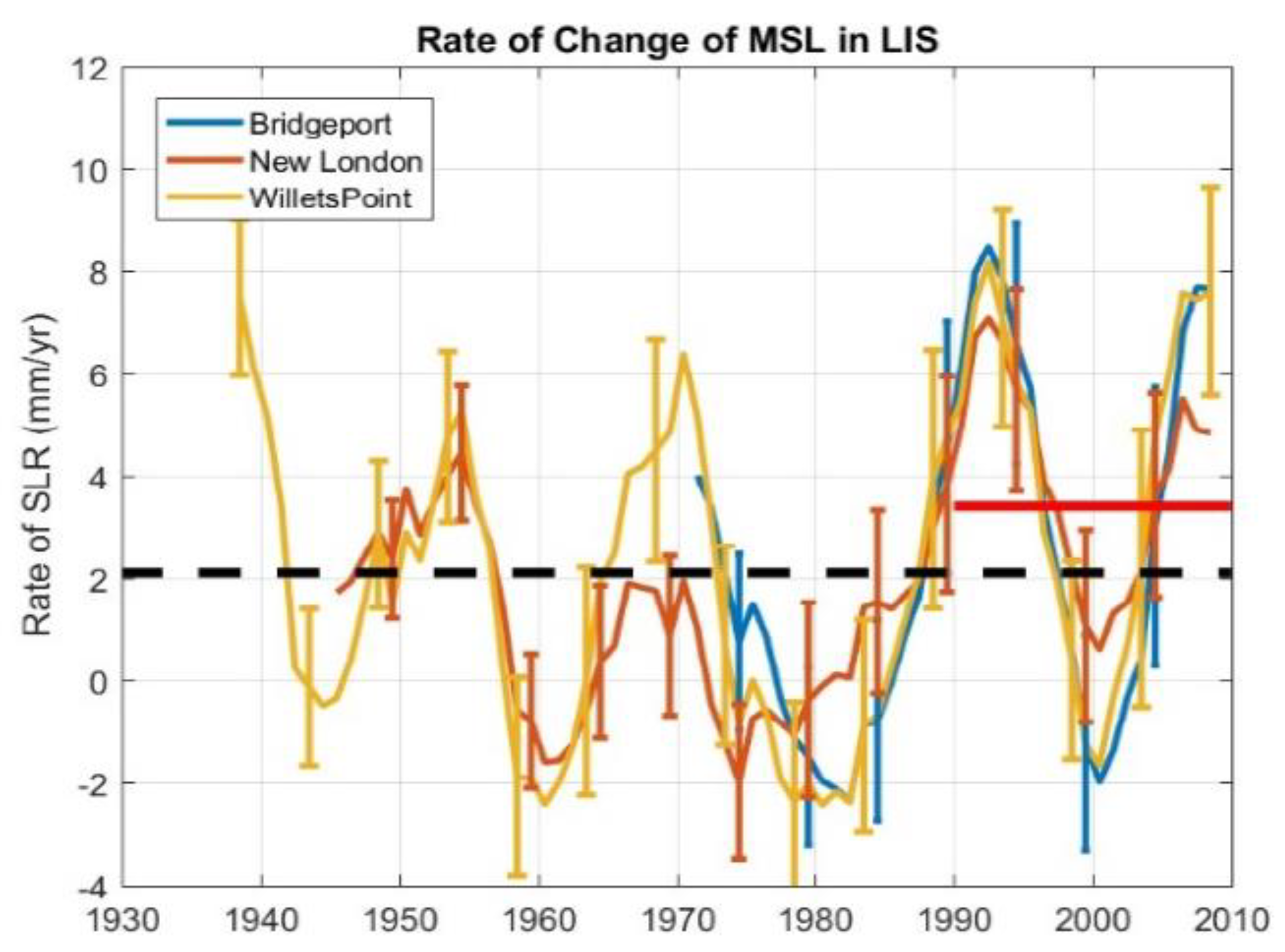
The Intergovernmental Panel on Climate Change (IPCC) estimates that the global mean sea level rose by 17 cm in the 20th Century. They also report an observed increase in the rate of global mean SLR over the 20th Century. The average rate from 1961 to 2003 was 1.8 mm/year, while the rate from 1993 to 2003 was 3.1 mm/year. Also, in Connecticut, relative SLR has been estimated at about 2.25 mm/year in New London over the period 1938-2006 (69 years) and 2.56 mm/year over the period 1964-2006 (43 years) (Clough J. et al., 2016). A recent study by Connecticut Institute for Resilience & Climate Adaptation (CIRCA) suggests an average SLR of 2.3 mm/year since 1930 to 2008 (long-term) and 3.4 mm/year since 1990 to 2008 (short-term average) based on recorded data in recent years in New London, Bridgeport and Willetspoint, (O’Donnell, 2017). Generally, an SLR of 2.25 to 3.4 mm/year is used in most literature for SLR in Connecticut.
Figure 11.
Rate of SLR in Long Island Sound (O’Donnell, 2017). The black dashed line indicates long-term average since 1930 and redline indicates short-term average of SLR from 1990.
Figure 11.
Rate of SLR in Long Island Sound (O’Donnell, 2017). The black dashed line indicates long-term average since 1930 and redline indicates short-term average of SLR from 1990.
3.3. Accretion Rates
Buckley et al. (2016) measured the salt marsh accretion rate at six sites in Long Island Sound. They used three models for determining current accretion rates. The results indicate that average accretion rates have increased in recent years, Table 6. The historical data represent an accretion of 0.11 to 0.50 cm/year for salt marshes in Long Island Sound. The results of three models on six salt marshes in Connecticut suggest an increase in the average accretion rate of salt marshes, Figure 13. As mentioned before, Buckley et al. (2016) assumed an average relative SLR of 0.69 to 0.75 cm/year and suggested that the relative SLR is 2 to 3X slower than the rates of current relative SLR. Nevertheless, this SLR is three to four times higher than regional historical rates and the current global average.
In 2013, the Sea Level Affecting Marshes Model (SLAMM) was established to identify potential responses of Connecticut’s coastal marshes and adjacent upland areas to anticipated increases in mean-tide water level elevations (Clough J. et al., 2016). Figure 14 shows the location of available accretion data which are used for the SLAMM model. The data of this model also represents an average accretion rate of 3.1 mm/year for study sites. This value is larger than the long-term (2.3 mm/year) and slightly smaller than the short-term (3.4 mm/year) SLR rate in Connecticut.
In addition, the nutrient concentration in LIS marshes is going from the west (high) to the east (low), which directly influences organic accretion rates (Buckley et al., 2016). The western marshes have higher organic accretion rates than the eastern marshes in LIS.
Figure 12.
Red stars indicate the site location of accretion rate samples for Buckley et al. (2016) project.
Figure 12.
Red stars indicate the site location of accretion rate samples for Buckley et al. (2016) project.
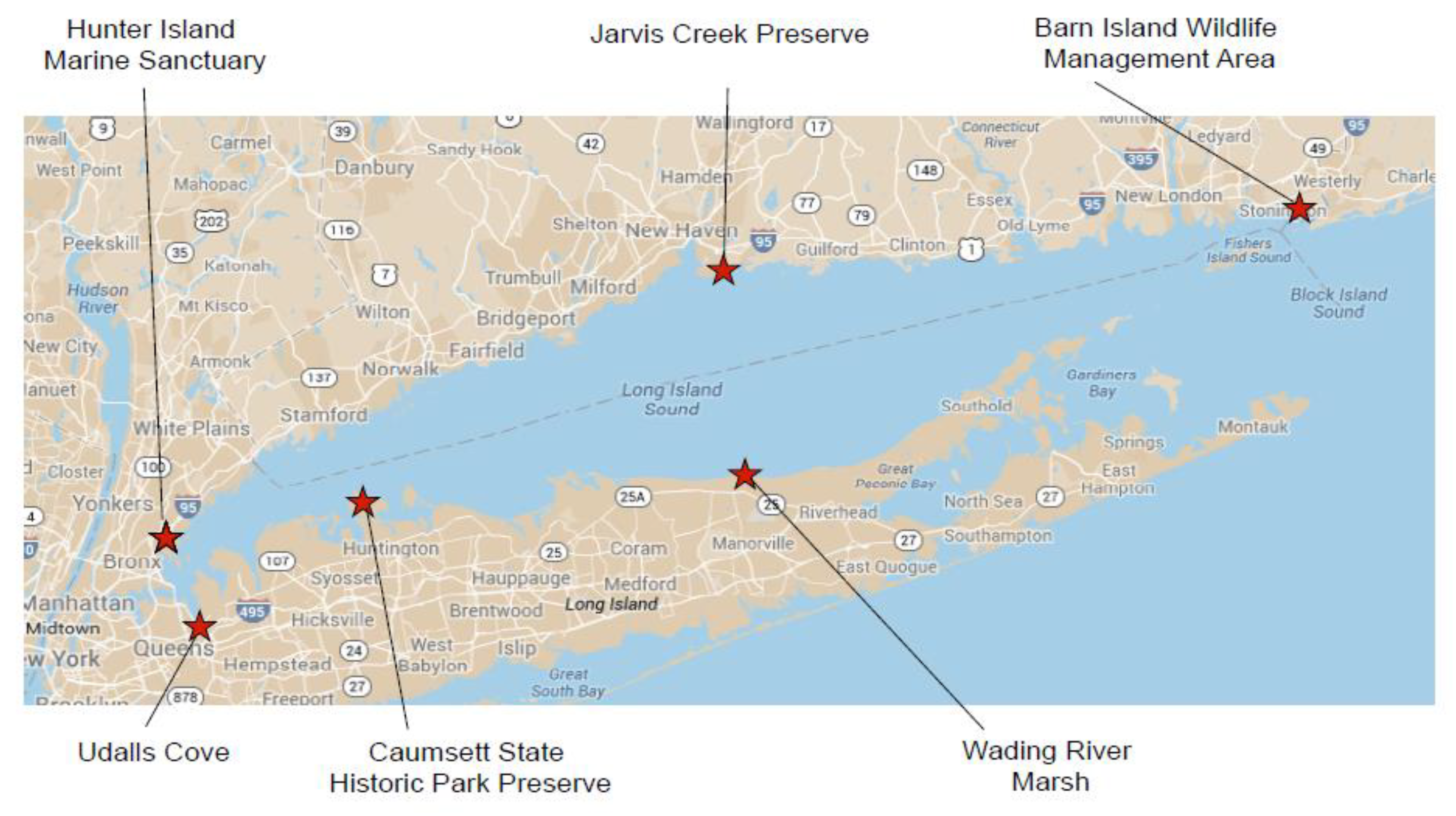

Table 6.
The accretion rates for six of Connecticut’s marshes (Buckley et al., 2016), The results represent an increase in salt marsh accretion rates, but the pace of increase in accretion rates is less than the pace of increase in Relative SLR. (HI=Hunter Island, UC=Udalls Cove, JC=Jarvis Creek, CP=Caumsett Park, BI=Barn Island, WR=Wading River).
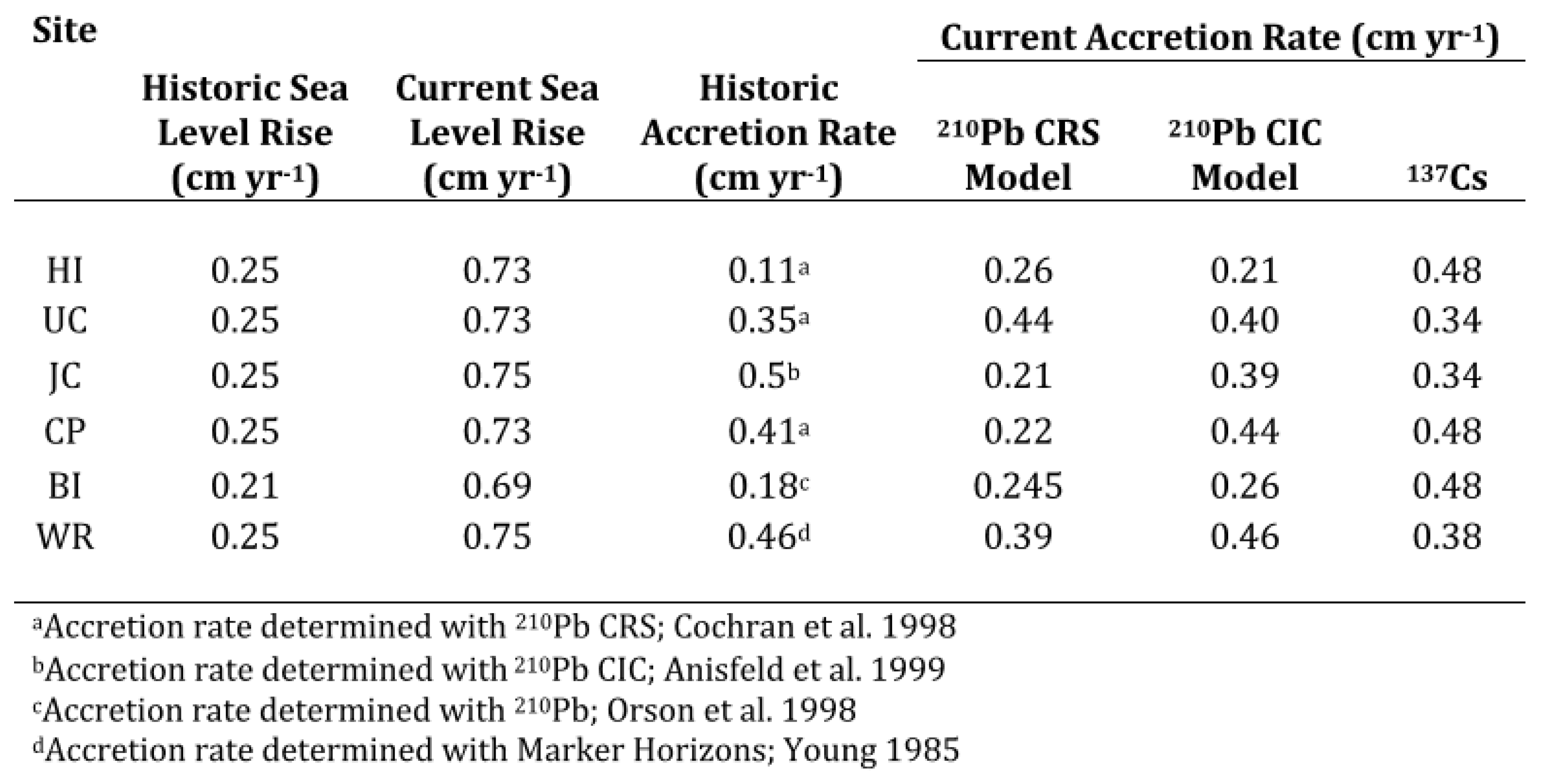
Figure 13.
Accretion rates have been increased by SLR, (Buckley et al., 2016). With accelerating SLR in recent years, the increasing accretion rates of the salt marshes (HI=Hunter Island, UC=Udalls Cove, JC=Jarvis Creek, CP=Caumsett Park, BI=Barn Island, WR=Wading River).
Figure 13.
Accretion rates have been increased by SLR, (Buckley et al., 2016). With accelerating SLR in recent years, the increasing accretion rates of the salt marshes (HI=Hunter Island, UC=Udalls Cove, JC=Jarvis Creek, CP=Caumsett Park, BI=Barn Island, WR=Wading River).
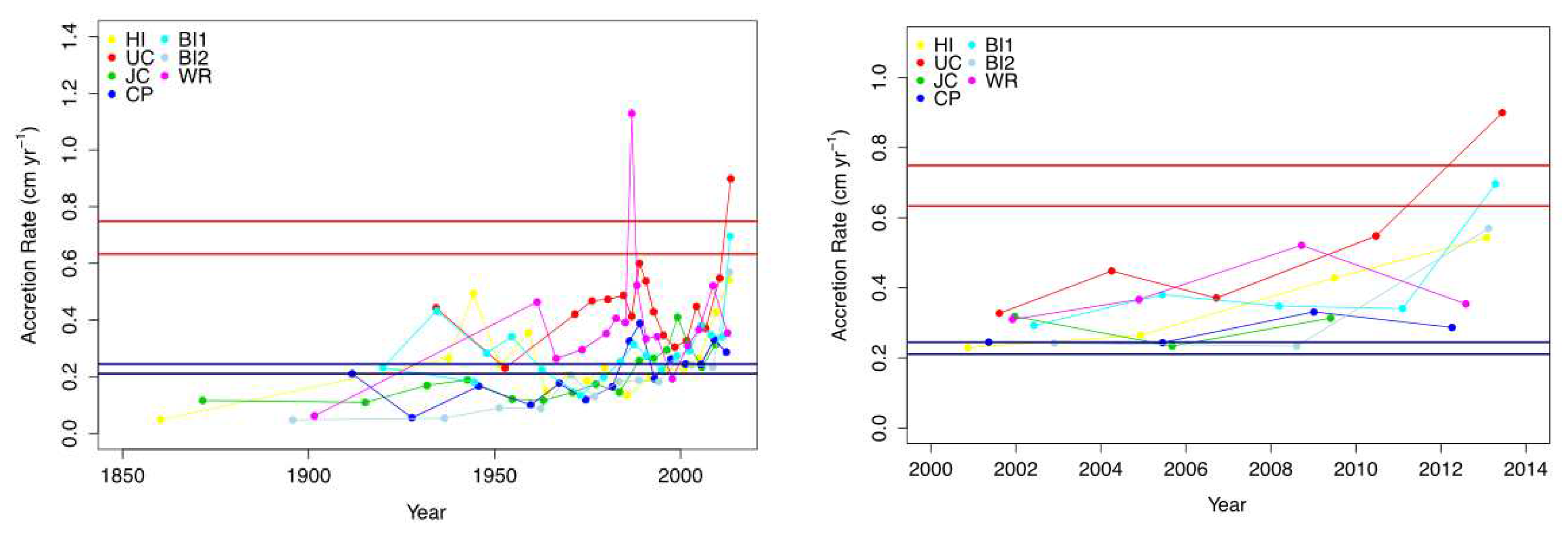
Figure 14.
Locations of Available Accretion Data in SLAMM model. (Yellow dots) (Clough J. et al., 2016).
Figure 14.
Locations of Available Accretion Data in SLAMM model. (Yellow dots) (Clough J. et al., 2016).

3.4. The Resiliency of Connecticut Marshes
So far, lots of research has been performed about the vulnerability of SLR on the marsh. However, recent studies argue that the Seal Level rise vulnerability for salt marsh is overstated (Kirwan et al., 2016). It has been shown that in Connecticut, the current average accretion rate is larger than the long-term average SLR and it’s close to the short-term average SLR. This represents that SLR is not the main stressor for salt marsh in Connecticut. Other recent literature also suggests that existing marshes in Connecticut are predicted to be capable of keeping up with current SLR, and marsh losses observed in the last 40 years may be due to reasons beyond SLR, mostly local anthropogenic reasons, such as nutrient load, boat traffic, or development, (Clough J. et al., 2016). By the way, more investigations are required to understand the main salt marsh stressors in Connecticut.
Another important point is that marsh sustainability highly depends on local physical, geological, and ecological conditions. Some marshes in Connecticut have very low accretion rates (less than 2mm/year), and some others have very large ones (more than 5mm/year). This represents that the sustainability and resiliency of each marsh should be studied separately. A similar approach must be taken into account for establishing an ecosystem-based protection system by marsh. Local sediment supply, tidal amplitude, upland slope and anthropogenic activity should be studied to generate an ecological-based protection system.
4. Coastal Protection by Marsh
The response of marshes to some coastal phenomena and the conditions for resiliency has been reviewed. In addition, an investigation was performed on available data for Connecticut marshes to understand current conditions, important stressors, and resiliency of the marshes. In this section, feasible studies will be performed for establishing an ecosystem-based coastal defense system at two sites on the Connecticut coastline Chittenden Park in Guilford and Short Beach in Stratford.
In order to have a successful and sustainable salt marsh for erosion control, a low wave energy area must be provided for marsh growth, the majority of sea-wave energy attenuates at a few 10 meters of marsh edge. Therefore it’s not usually required to develop a wide wetland for erosion control purposes. Moreover, sediment supply must be enough to guarantee an accretion rate equal to or larger than the SLR rate. Finally, it is crucial to create a gentle slope in the upland area to ease marsh migration.
Before analyzing the coastlines, wind and wave conditions in Long Island Sound will be reviewed. The central long island sound buoy with coordinates 41°8'15" N 72°39'18" W, owned and maintained by UCONN, was used to analyze wind and wave conditions in Long Island Sound. The majority of winds blow from the west, while the average wind speed of northern winds is more than the southern ones (Figure 15). Given the long west-east fetch and short north-south fetch in LIS (Figure 16), the dominant wave direction in the deep part of LIS must be from the west and northwest. Therefore, the southern coastline of LIS (New York coast) should experience more energy than the northern coastlines (Connecticut).
4.1. Chittenden Park, Guilford, CT
Chittenden Park, located in east Connecticut, is surrounded by the West River at the west and a headland at the east side. As the coastline is protected by headlands in both west and east sides, the fetch length is limited in the area; therefore, the dominant waves from the west would not affect the coastline directly and just some diffracted southwest waves can reach the coastline, Figure 17. Maximum fetch length is about 35km and although wave energy is limited in the area, marshes still need protection. Marshes cannot tolerate high energy waves and a calm condition must be provided for growing marsh which would be established for erosion control purposes.
Using Google Earth’s historical satellite images, the current coastline condition was investigated. The oldest available satellite image of Google Erath (04/22/1990) and the newest one (04/20/2016) was studied to figure out coastline evolution in 16 years, Figure 18. The results indicate high erosion conditions in the area. More than 8000m2 of the coastline has vanished in 16 years. The coastline includes a combination of consecutive non-vegetated and vegetated coastlines. The vegetated part seems to survive the part of an old coastal salt marsh which is eroding gradually. The majority of erosion took place in non-vegetated parts of the coastline and the vegetated had not been eroded as much as the non-vegetated coast. According to the two digital areal images, before (3/29/2012) and after (9/19/2010), the majority of erosion in the vegetated part happened during Hurricane Sandy, Figure 19. This represents that vegetated areas can be used for erosion protection in usual conditions, but they should be protected from extreme storms. It can be seen from the images that the gradual erosion of the remaining salt marsh has not stopped after Sandy; therefore, they must be protected before they completely disappear.
The presence of rocky headlands in the adjacent area represents the lack of sediment sources and it seems that the West River is the only sediment source entering the system. However, the river has a small drainage area and it might not be able to inject enough sediment into the coastline to guarantee coastline resiliency. For designing an ecosystem-based system for the coastline, a comprehensive study should be done on the amount of sediment annually deposited from the river into the coastline, and it must be calculated how much of those sediments can be trapped by the ecosystem-based protection system.
In order to imply an artificial marsh on the coastline, it is crucial to attenuate the wave energy, which can be done by setting a group of reef balls or small detached breakwater in front of the coastline. These reef balls are sufficient to attenuate wave energy and they would be a suitable place for marine habitats to live (O’Donnell 2015), Figure 21. Furthermore, to depose sediments and stabilize the shoreline, some marshes must be set up on the coastline between the reef balls and the current beach, Figure 22. Again, the availability of sediment supplies is essential for the resiliency of salt marsh and the designed system must be able to accumulate sediments entering from West River.
4.2. Short Beach, Stratford, CT
Short Beach, located in Stratford at the southern Housatonic River mouth, is surrounded by a sandy beach at the north and a mixture of sand and gravel at the south. There is a rocky headland which has been protected by a revetment. Due to the existence of a detached breakwater in front of the coastline, the fetch is strongly limited and the maximum fetch length is about 2km from the north, Figure 23. Therefore, wave energy is strongly limited and tidal and river currents are the primary source of energy in the coastline. The existence of a sandy beach in the north demonstrates that there must be enough sediment sources from the north and the Housatonic River. In addition, the detached breakwater has been built to protect the navigation channel from waves, though it produced a calm condition for growing salt marsh and developing sandy beaches on the coastline.
The Google Earth satellite images were used to compare coastline variation between 04/11/1991 and 09/22/2015 (14 years) at the southern part of Short Beach. According to Figure 24, erosion happened on the coastline, excluding a small portion of the northern part. This coastline has a unique condition for establishing a coastal protection system by marsh due to the availability of sediment sources from the river and the low wave energy of the coastline.
This coastline used to be an ecological coastline for crabs to lay their eggs. However, because of erosion and washed-out sands, the number of horseshoe crabs has dropped significantly (Beekey et al. 2015). Therefore, a survival plan has been implemented since early 2015, including setting up a group of reef balls and salt marsh to trap finer and organic sediment and provide a suitable coastline for crabs to lay the eggs, Figure 25. There is no data on how the system has been designed, but the system is working well!
5. Conclusion
Salt marshes have proven to be effective in coastal protection due to their ability to attenuate waves, stabilize soil, and deposit sediments. The wave attenuation capacity of marshes generally increases with their length. Marsh edges dissipate high-frequency waves, such as sea waves, more effectively than low-frequency waves like swell waves. The roots of marsh vegetation play a crucial role in stabilizing the soil and preventing erosion by binding the soil particles together. It is worth noting that while salt marshes are effective in low wave energy conditions, they can be susceptible to erosion from large waves.
Moreover, salt marshes can also attenuate storm surges. However, it is important to consider that significant wetland areas are required for effective storm surge protection. Additionally, salt marshes have the ability to adapt to relative sea-level rise (SLR) through sediment accretion and upland migration. Ensuring sufficient sediment supply and a gentle upland slope are key factors for facilitating salt marsh adaptation to SLR.
To develop a sustainable and resilient coastal protection system using salt marshes, several considerations need to be taken into account. Creating a calm wave environment at the site can be achieved by constructing reef balls and submerged breakwaters on the seaward side of the marsh. Sufficient sediment supply is crucial to support the marsh's structure and adaptation to SLR. In cases where sediment supply is limited, a gentle upland slope becomes particularly important. Additionally, factors such as vegetation density, type, stiffness, as well as ecological factors like nutrient supply and vegetation disease, should be carefully considered in the design process.
Analyzing the Connecticut coastlines reveals that they have limited wave energy due to their short fetch length, which is advantageous for salt marsh growth. Historical data suggests that the total acreage of Connecticut salt marshes is either stable or increasing, and average accretion rates align closely with current SLR, indicating that Connecticut marshes are keeping pace with the current rate of sea-level rise.
A feasibility study was conducted on two Connecticut coastlines, Chittenden Park in Guilford and Short Beach in Stratford. Although wave energy is generally limited along Connecticut coastlines, the assessment of fetch length and dominant wind directions indicates that Short Beach experiences even lower wave energy compared to Chittenden Park. Determining sediment availability in specific coastlines is complex due to the non-uniform form of Connecticut's coastline. However, preliminary observations suggest that sediment availability may be higher in Short Beach compared to Chittenden Park, but further measurements and studies are necessary. Comparison of satellite images indicates that erosion is more severe in Chittenden Park than in Short Beach, with hurricane Sandy being the main driver of intense erosion in the former coastline.
References
- Akan, A. O. (2006). Amsterdam; Boston: Oxford [England]; Burlington, Mass.: Elsevier; Butterworth-Heinemann.
- Basso G., O’Brien K., Albino Hegeman M. and O’Neill V., (2015). Status and trends of wetlands in the Long Island Sound Area: 130 year assessment. U.S. Department of the Interior, Fish and Wildlife Service. (36 p.).
- Beekey M.A., Mattei J. H., (2015), The Mismanagement of Limulus polyphemus in Long Island Sound, U.S.A.: What Are the Characteristics of a Population in Decline?, Changing Global Perspectives on Horseshoe Crab Biology, Conservation and Management, pp 433-461. [CrossRef]
- Browne, M.A., Chapman, M.G., (2014). Mitigating against the loss of species by adding artificial intertidal pools to existing seawalls. Mar. Ecol. Prog. Ser. 497, 119–129. [CrossRef]
- Buckley S., Al--Haj A., Fulweiler R. (2016) Sentinels of Change — Are Salt Marshes in LIS Keeping Pace with Sea Level Rise?, Boston University, U.S. Environmental Protection Agency.
- Clough J., Polaczyk A., Propato M. (2016) Advancing Existing Assessment of Connecticut Marshes’ Response to SLR, U.S. Fish and Wildlife Service, Northeast Regional Oceans Council, Connecticut, Warren Pinnacle Counmsulting,.
- Gedan, K.B., Kirwan, M.L., Wolanski, E. et al., (2011), The present and future role of coastal wetland vegetation in protecting shorelines: answering recent, challenges to the paradigm Climatic Change, 106: 7. 106, 7. [CrossRef]
- Gittman, R.K., Popowich, A.M., Bruno, J.F., Peterson, C.H., (2014). Marshes with and without sills protect estuarine shorelines from erosion better than bulkheads during a Category 1 hurricane. Ocean Coast. Manage. 102, 94–102. [CrossRef]
- Hill, T.D., and S. C. Anisfeld (2015), Coastal wetland response to sea level rise in Connecticut and New York, Estuarine Coastal Shelf Sci., 163, 185–193. [CrossRef]
- Jadhav R.S., Chen Q., Smith J.M. (2013) Spectral distribution of wave energy dissipation by salt marsh vegetation, Coastal Engineering, Vol 77, Pages 99–107. [CrossRef]
- Kirwan, M. L., G. R. Guntenspergen, A. D’Alpaos, J. T. Morris, S. M. Mudd, and S. Temmerman (2010), Limits on the adaptability of coastal marshes to rising sea level, Geophys. Res. Lett., 37, L23401. [CrossRef]
- Kirwan, M. L., D. C. Walters, W. G. Reay, and J. A. Carr (2016), Sea level driven marsh expansion in a coupled model of marsh erosion and migration, Geophys. Res. Lett., 43, 4366–4373. [CrossRef]
- Kirwan, M. L., and J. P. Megonigal (2013), Tidal wetland stability in the face of human impacts and sea-level rise, Nature, 504, 53–60. [CrossRef]
- Kirwan, M. L., Temmerman, S., Guntenspergen G R., Fagherazzi S., (2016), Overestimation of marsh vulnerability to sea level rise. Nature Climate Change, 6, 253–260. [CrossRef]
- Moller, I., Kudella, M., Rupprecht, F., Spencer, T., Paul, M., van Wesenbeeck, B., Wolters, k., Jensen, G., Bouma, K., Miranda- Lange, T.J., Schimmels, M.S., (2014). Wave attenuation over coastal salt marshes under storm surge conditions. Nat. Geosci. 7, 727–731. [CrossRef]
- http://www.ct.gov/deep/cwp/view.asp?a=2705&q=475764&deepNav_GID=2022.
- (a).
- O'Donnell J. (2017), Sea Level Rise and Coastal Flood Risk in Connecticut, Department of Marine Sciences & Connecticut Institute for Resilience and Climate Adaptation, The University of Connecticut.
- Shepard CC, Crain CM, Beck MW (2011) The Protective Role of Coastal Marshes: A Systematic Review and Meta-analysis. PLoS ONE 6(11): e27374. [CrossRef]
- Sutton-Grier A.E., Wowk K., Bamford H., (2015). Future of our coasts: The potential for natural and hybrid infrastructure to enhance the resilience of our coastal communities, economies and ecosystems, Environmental Science & Policy, 51, P 137–148. [CrossRef]
- Temmerman, S., P. Meire, T. J. Bouma, P. M. J. Herman, T. Ysebaert, and H. J. De Vriend (2013), Ecosystem-based coastal defence in the face of global change, Nature, 504, 79–83. [CrossRef]
- Tiner, R.W., I.J. Huber, T. Nuerminger, and E. Marshall. (2006). Salt Marsh Trends in Selected Estuaries of Southwestern Connecticut. U.S. Fish and Wildlife Service, National Wetlands Inventory Program, Northeast Region, Hadley, MA. Prepared for the Long Island Studies Program, Connecticut Department of Environmental Protection, Hartford, CT. NWI Cooperative Report. 20 pp.
- www.un.org/esa/sustdev/natlinfo/indicators/...sheets/...coasts/pop_coastal_areas.pdf, UN, Division for Sustainable Development.
Figure 1.
Wave attenuation rates through salt marsh vegetation versus marsh transect length, (Shepard et al., 2011). Marsh transcect length is the distance in marsh that wave was measured along it. Wave attenuation rates generally increase with marsh length, but increasing rate is less for wave high larger than 0.5 meter.
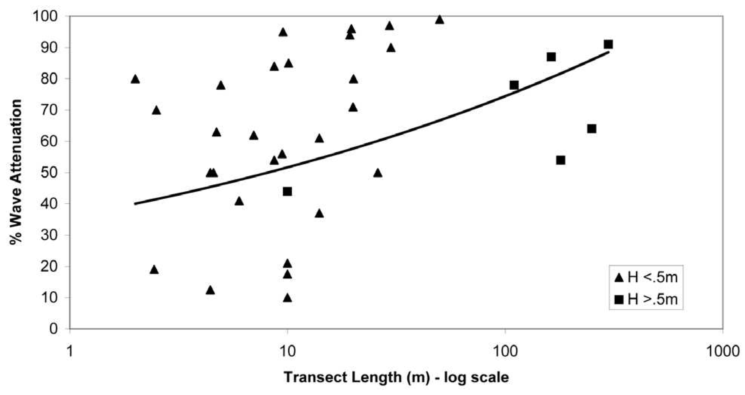
Figure 2.
The factors most quoted as being of importance to the wave attenuation capacity of salt marsh vegetation, (Shepard et al., 2011).
Figure 2.
The factors most quoted as being of importance to the wave attenuation capacity of salt marsh vegetation, (Shepard et al., 2011).
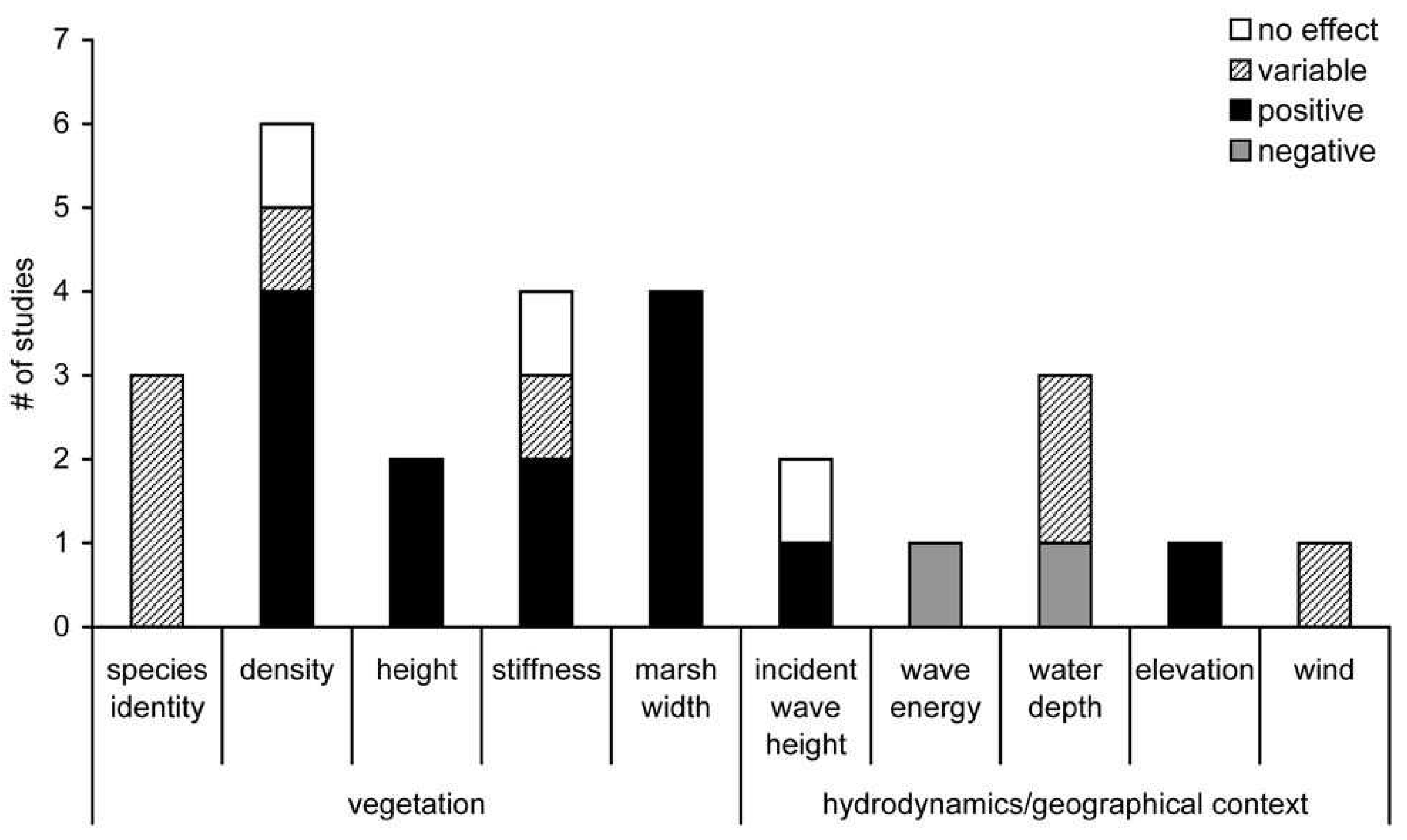
Figure 3.
Wetland reclamation increases the risk of coastal flood disasters (Temmerman et al., 2013). blue arrows indicate an increase or decrease in the intensity of storm wave and orange lines indicates a conventional engineering system (e.g., sea walls, revetments). Left: a conventional (traditional) engineering system, Right: an ecosystem-based defense by marsh.
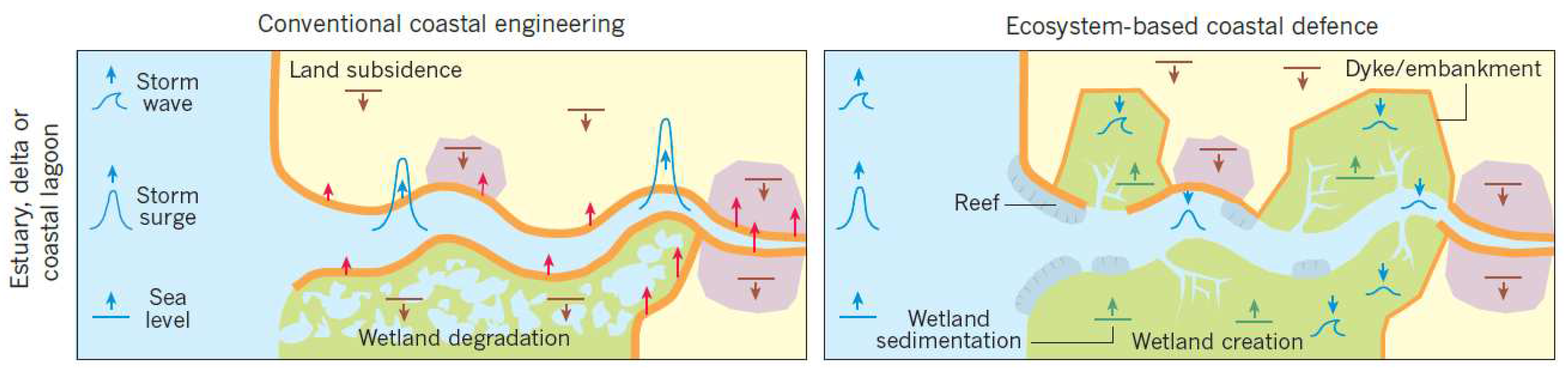
Figure 4.
The relationship of measured wave attenuation r with, a: traversed distance across which it is measured, and b: the ratio of water depth to vegetation height, (Gedan et al., 2011). Ratios greater than 1, indicated by a dashed line, indicate the wetland vegetation was submerged during measurement. (r is equal to the proportion of wave reduction per meter of land traversed).
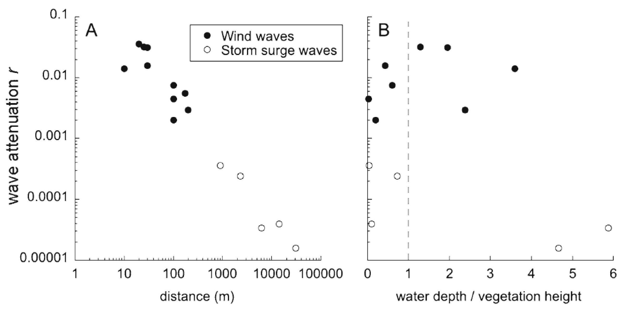
Figure 5.
Marsh edge erosion, the vegetated marsh platform, and marsh migration into adjacent forested uplands, SLR increases the depth and wave energy at the marsh edge. This can lead to marsh edge erosion. Simultaneously, it would increase soil building and the accretion rate of the marsh. In addition, the marsh migrates to the upland and forest.
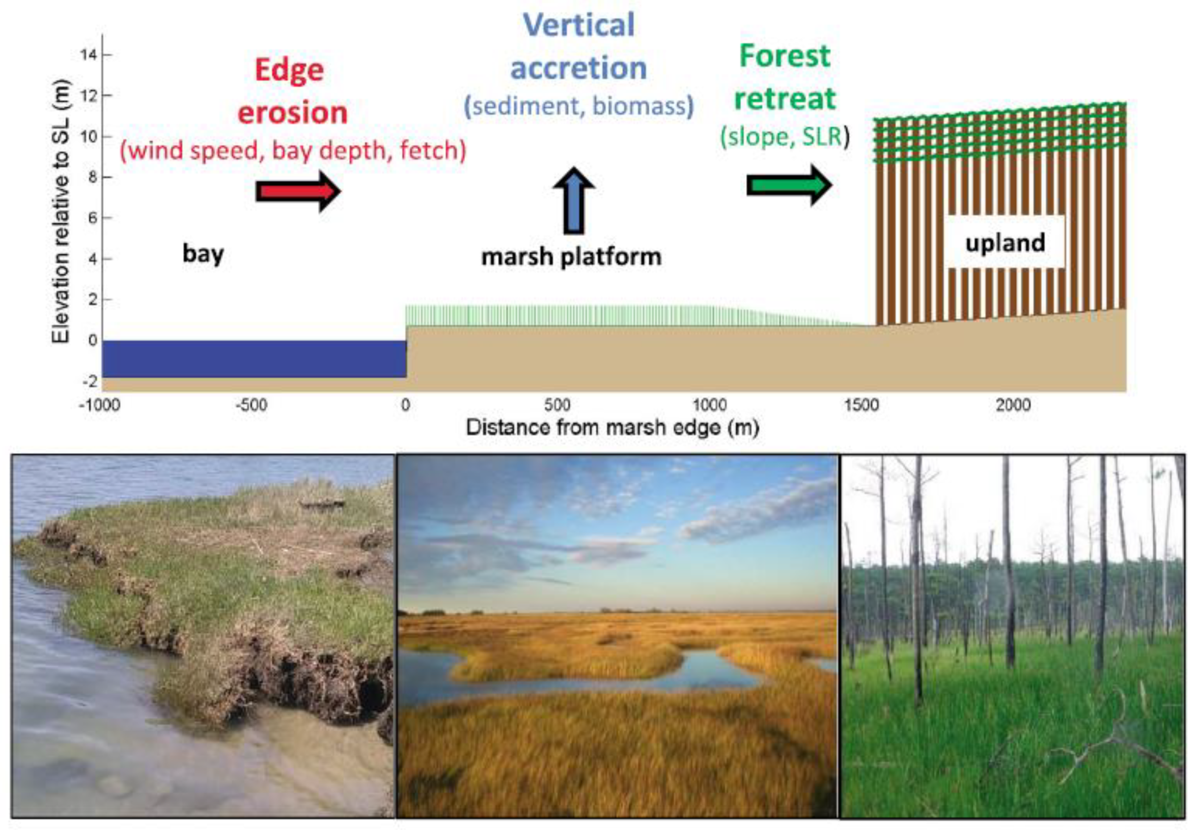
Figure 6.
a: Organic and mineral matter accretion increase at a low rate of SLR in a sediment-deficient marsh. As the rate of SLR exceeds a threshold level, the contribution of organic matter in total accretion decrease. b: the threshold rate of sea-level rise tends to be a function of sediment availability and beyond that, marshes cannot survive.
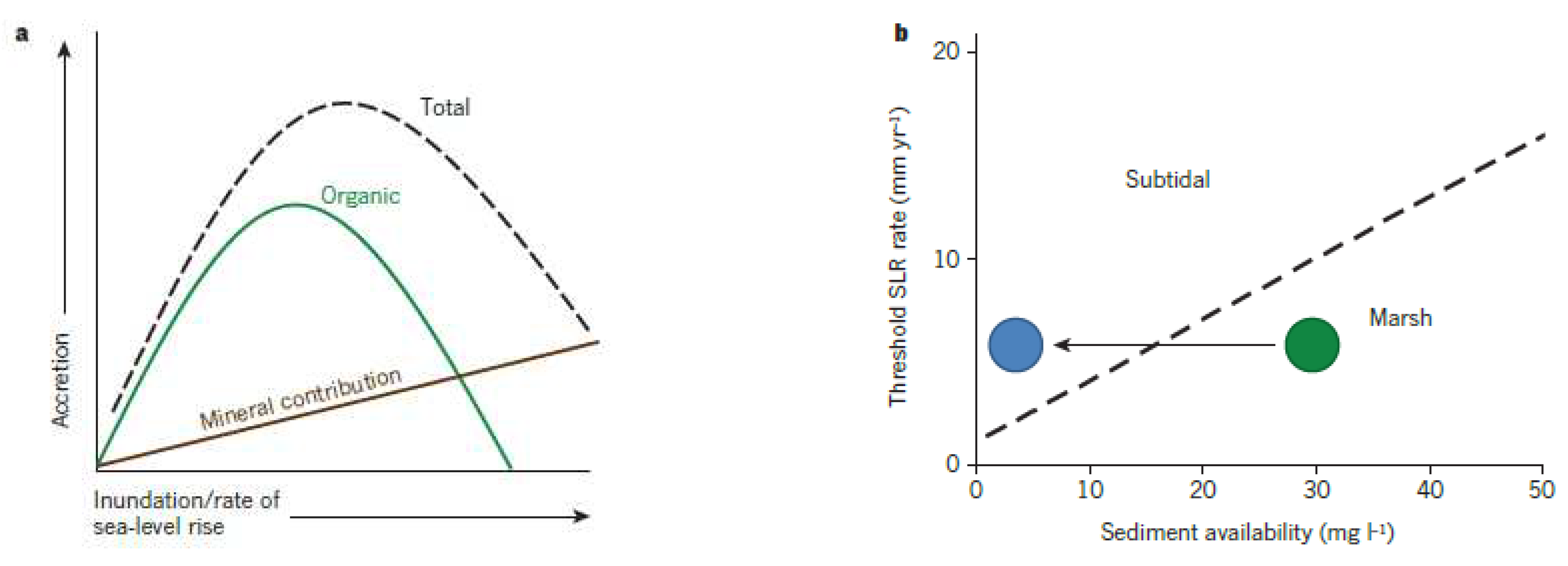
Figure 7.
(a–c) Phase diagrams illustrating the dependence of lateral marsh evolution on relative SLR and sediment supply (SSC) and its sensitivity to the slope of adjacent uplands. Colors represent the rate of change in marsh width (dMW/dt) averaged over a 150-year simulation, where blues indicate a rapid decrease in marsh width and reds indicate a rapid increase in marsh width. Figure 7a shows a gentle upland slope (0.001) representative of coastal plains, Figure 7b shows a moderate upland slope (0.01) representative of glaciated coasts, and Figure 7c shows a steep upland slope (0.2) representative of active margin coasts. The phase boundary between marsh contraction and marsh expansion moves toward higher SLR rates and SSC between Figure 7a–7c, indicating that the potential for net marsh expansion decreases with increasing upland slope. (d) Marsh expansion rate as a function of SLR for a variety of upland slopes and a single external sediment supply (40mg L_1). Increasing SLR rates lead to increasing marsh expansion rates until a threshold SLR rate is exceeded and drowning occurs. The steep upland slope example implicitly represents a “no migration” scenario associated with hardened (Kirwan et al., 2016).
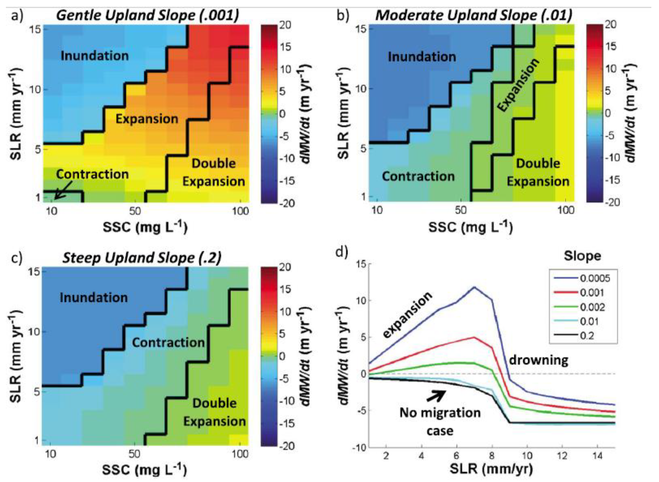
Figure 8.
a man-made wetland for flood protection, Scheldt estuary, Belgium, (Temmerman et al., 2013), this man-made system protects more landward, densely populated areas from storm surge flooding. For flood protection purposes, a large space is required to develop an ecosystem-base system. It usually hard to find such a space near a metropolitan area.
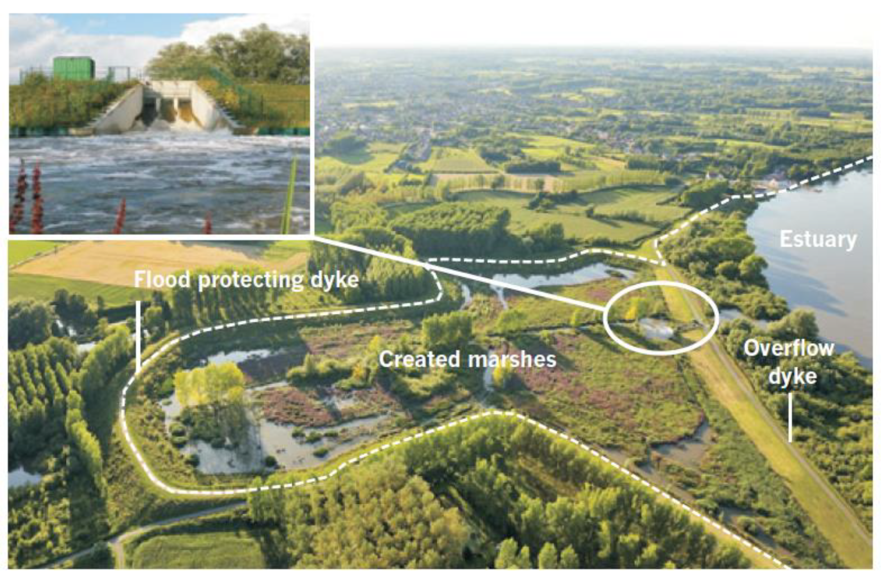
Figure 9.
Location of study estuaries along the Connecticut coast by Tiner et al. (2006).
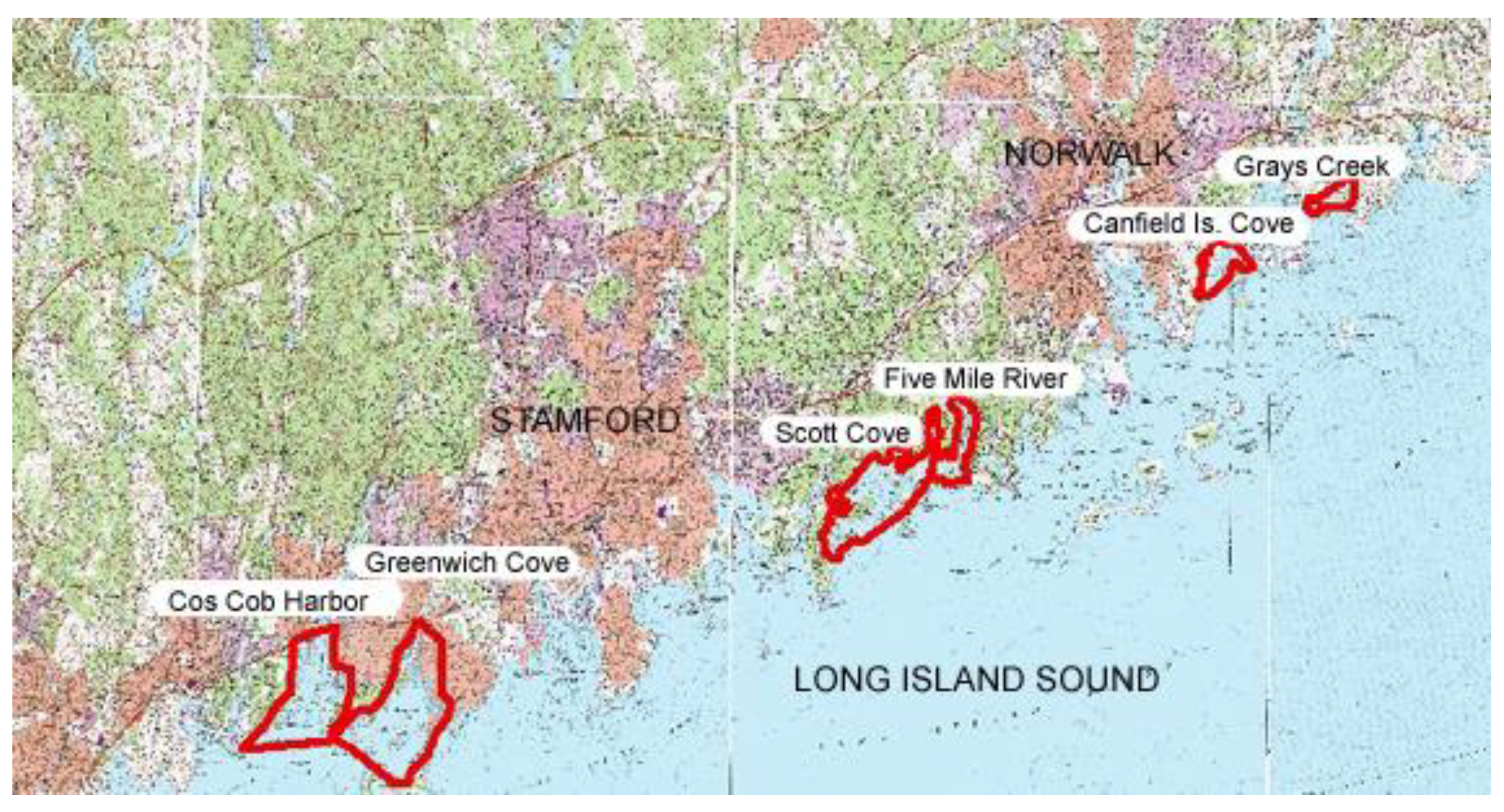
Figure 10.
Loss of low marsh, a slight loss in high marsh, and a huge gain in tidal flat areas in six salt marshes of western Connecticut (Tiner et al., 2006). All salt marshes experienced a loss in low marshes and gain in tidal flat from 1974 to 2004.
Figure 10.
Loss of low marsh, a slight loss in high marsh, and a huge gain in tidal flat areas in six salt marshes of western Connecticut (Tiner et al., 2006). All salt marshes experienced a loss in low marshes and gain in tidal flat from 1974 to 2004.
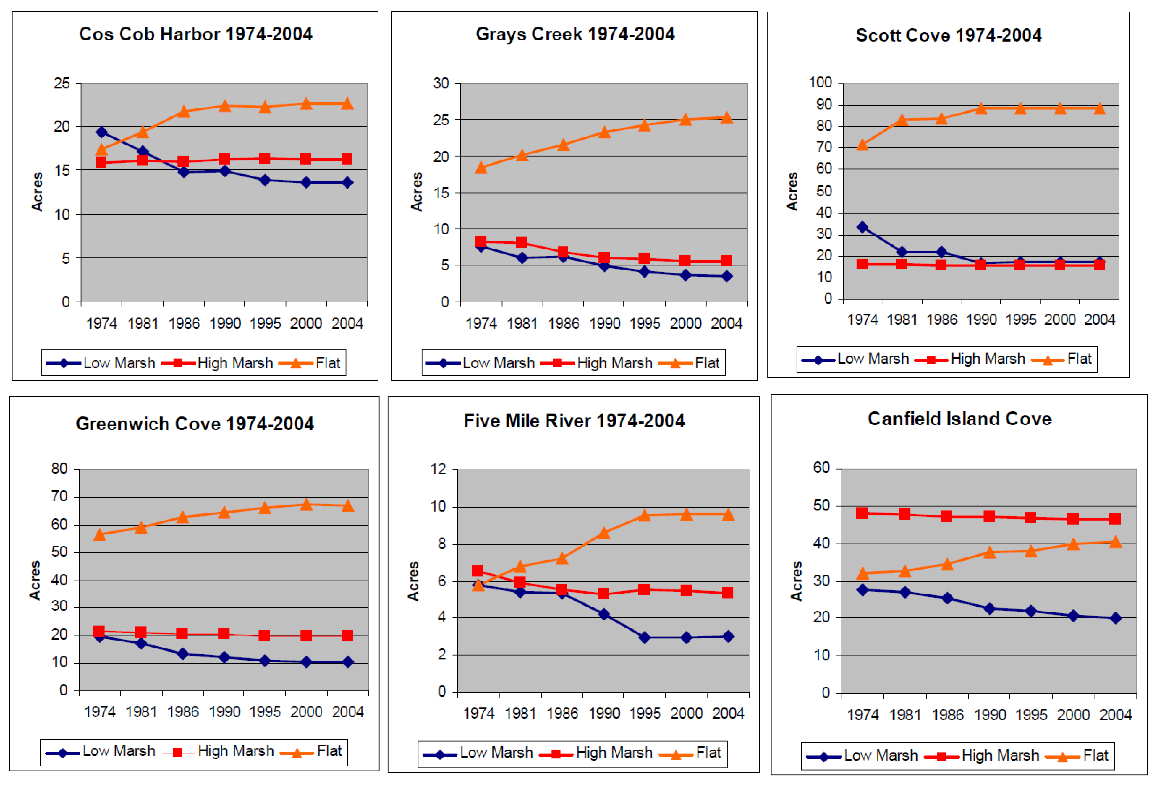
Figure 15.
Windrose for central Long Island Sound. The wind-rose indicates where the winds come from and the darkness of blue represents the average wind speed. The Prevailing wind directions in LIS are from northwest, west, and southwest with higher intensity (average wind speed for northwest winds).
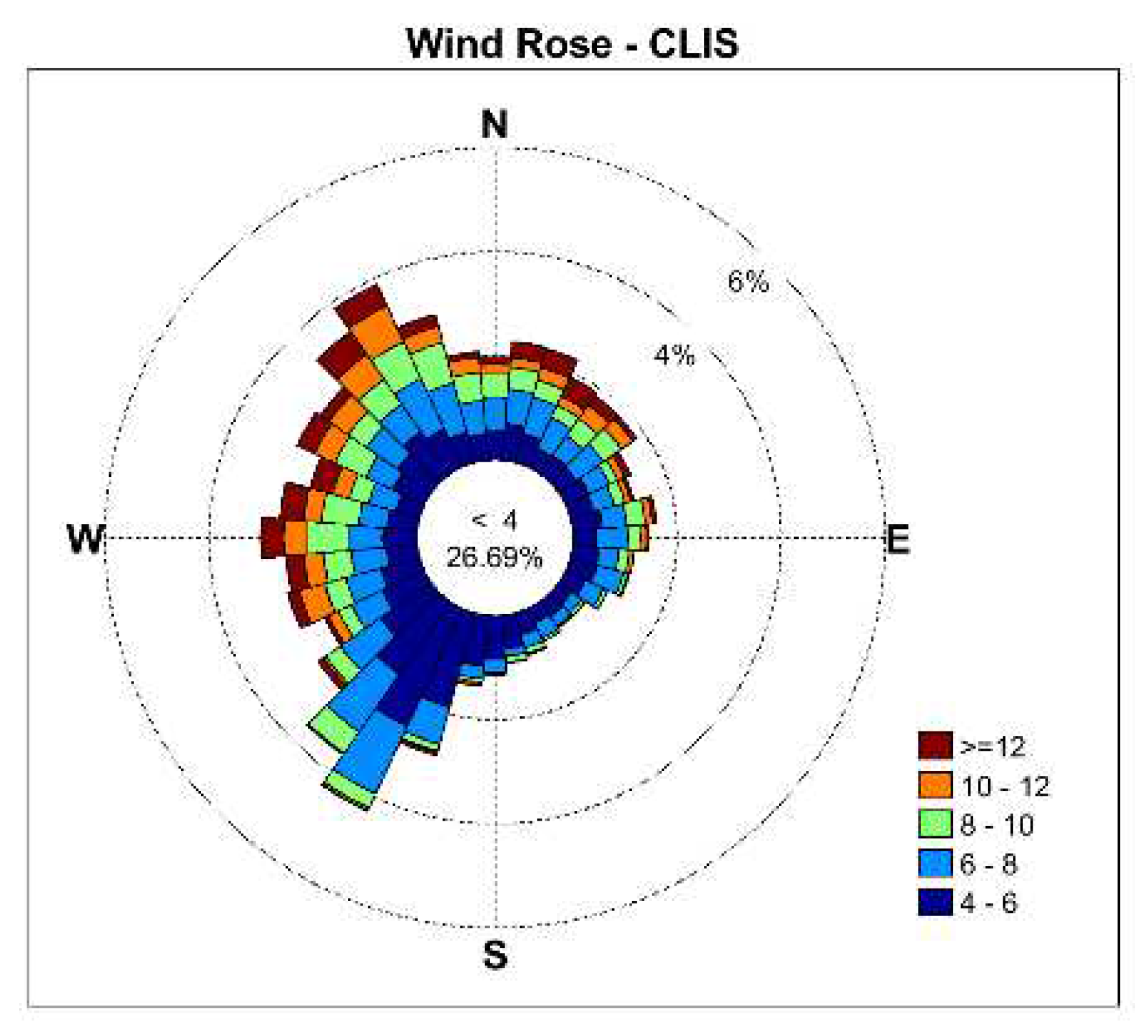
Figure 16.
Fetches distance and Buoy location in Long Island sounds; longest fetch has a west-east alignment with 140km.
Figure 16.
Fetches distance and Buoy location in Long Island sounds; longest fetch has a west-east alignment with 140km.
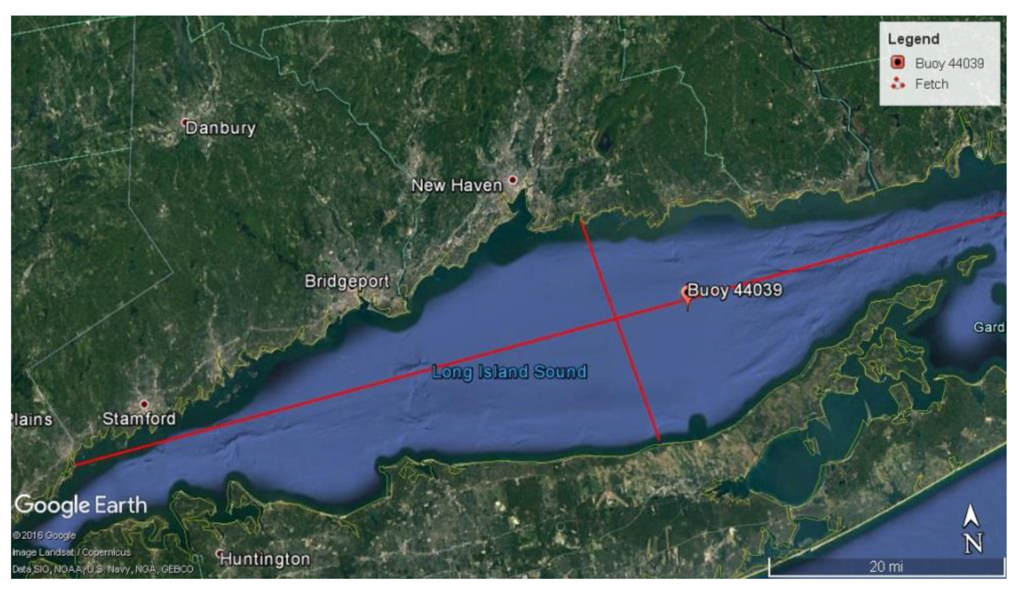
Figure 17.
Possible wave fetch for Chittenden Park, Guilford, the area is protected by eastern headlands; fetch length varies from 25km to 35km, the red line represent the fetch with the most intensive wind, however, the diffracted waves from this direction impact on Chittenden park coastline.
Figure 17.
Possible wave fetch for Chittenden Park, Guilford, the area is protected by eastern headlands; fetch length varies from 25km to 35km, the red line represent the fetch with the most intensive wind, however, the diffracted waves from this direction impact on Chittenden park coastline.
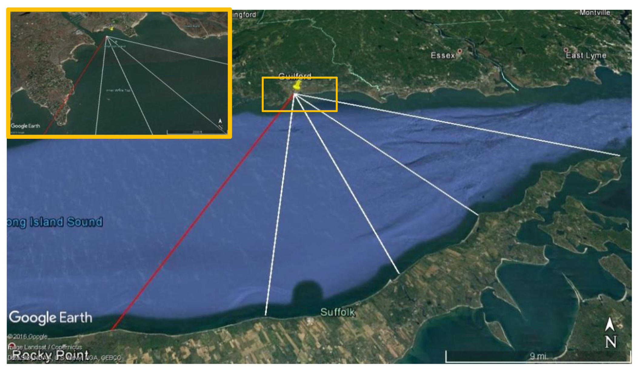
Figure 18.
Comparison of coastal variations between 04/22/1990 and 04/20/2016 (16 years) in Chittenden Park, Guilford, top left: 1990 image, top right: 2016 image, bottom: the comparison of two coastlines. More than 8000 m2 (88000 ft2) of the coastline was drawn and eroded in just 16 years.
Figure 18.
Comparison of coastal variations between 04/22/1990 and 04/20/2016 (16 years) in Chittenden Park, Guilford, top left: 1990 image, top right: 2016 image, bottom: the comparison of two coastlines. More than 8000 m2 (88000 ft2) of the coastline was drawn and eroded in just 16 years.
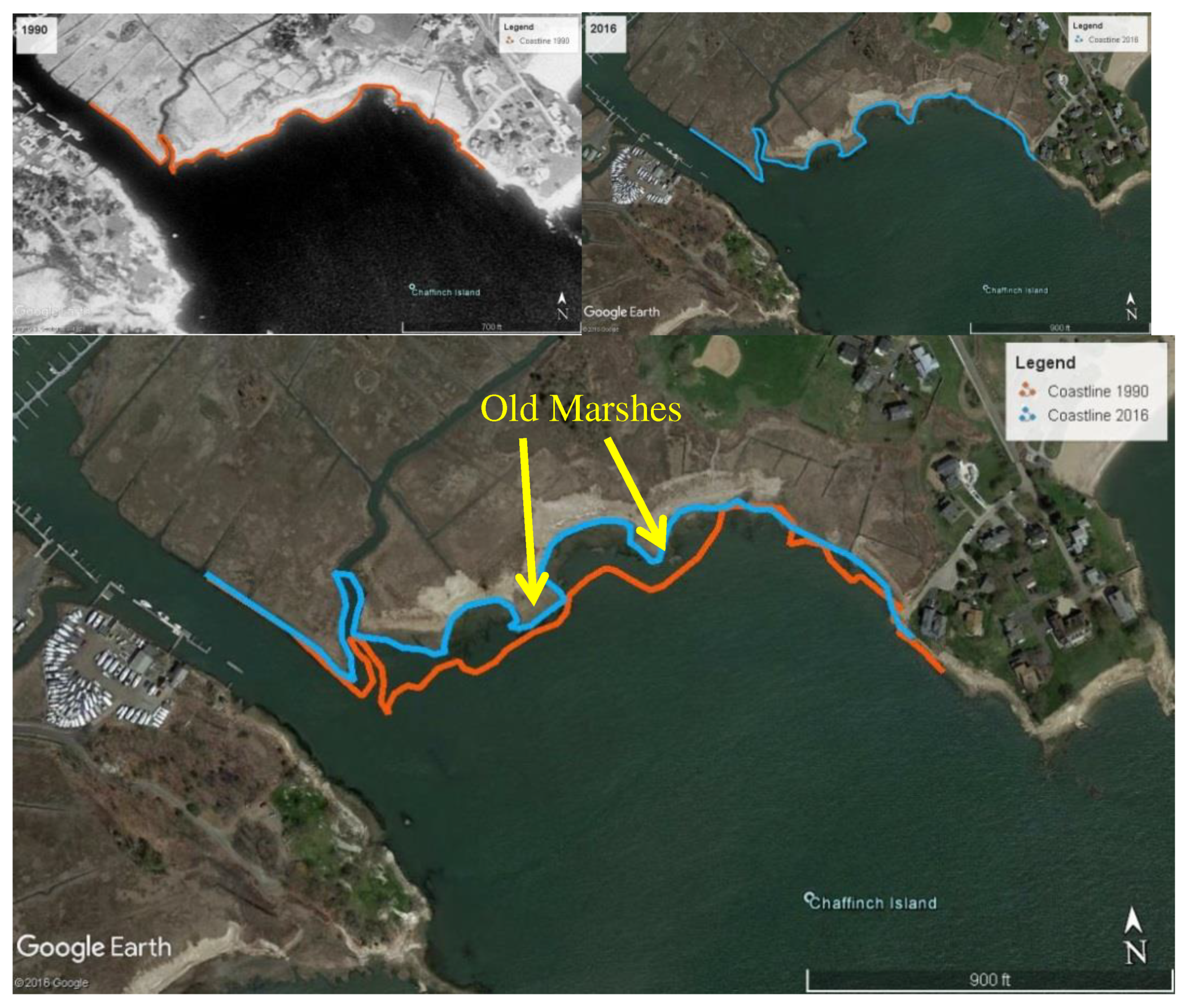
Figure 19.
Comparison of digital images, a: remained coastal salt marsh before (3/29/2012) and after (9/19/2010) hurricane Sandy, b: upland marsh erosion, 1990, 2008, before Sandy (3/29/2012), after Sandy (04/20/2016), 2016. Hurricane Sandy happened on 10/29/2012, Comparison shows that the majority of erosion in vegetated areas took place during hurricane Sandy.
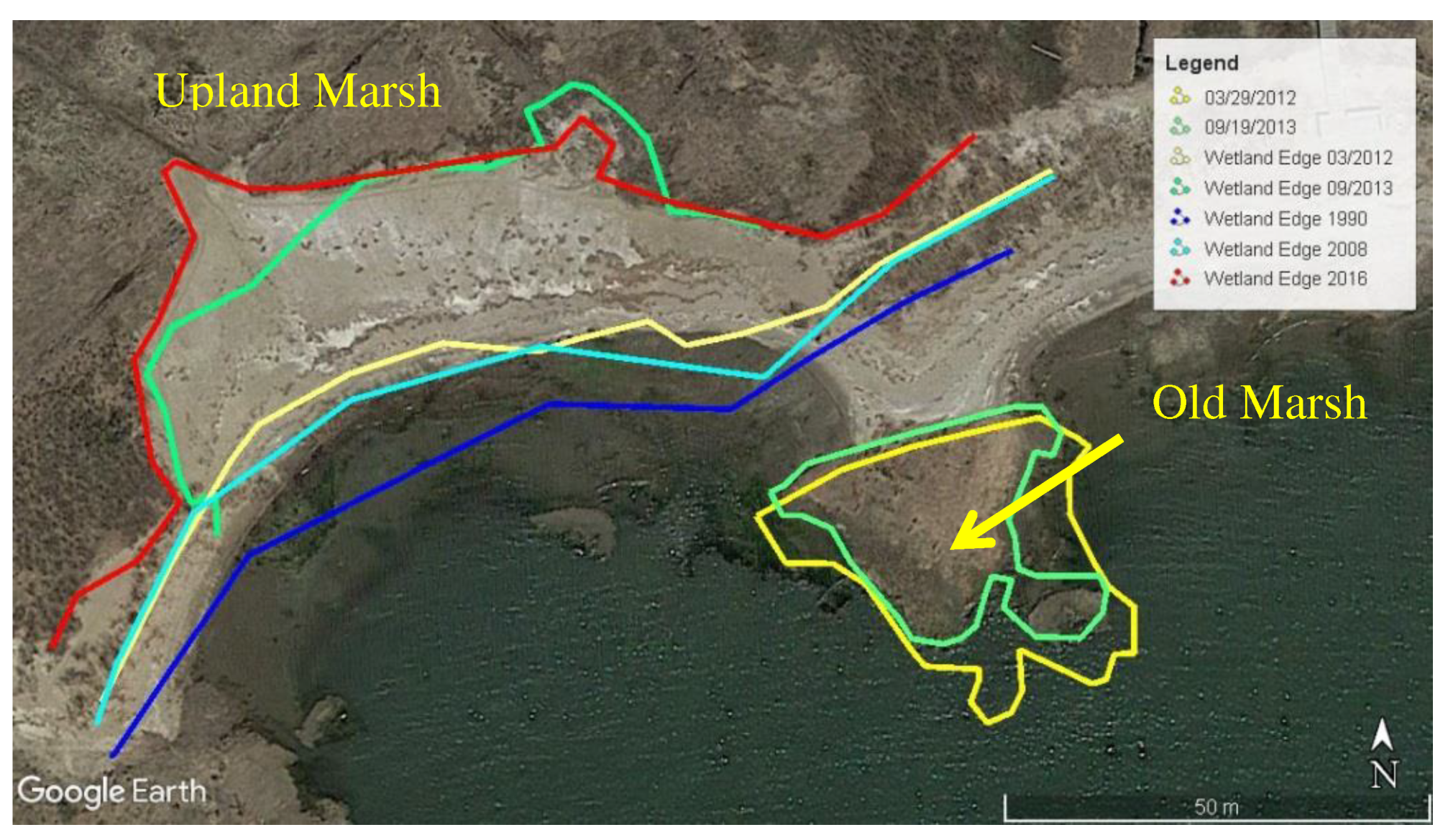
Figure 20.
Marsh edge loss based on digital images of 1990, 2008 and 2016, Marsh edge loss between 2008 and 2016 (8 years) is much larger than the period between 1990 and 2008 (16 years).
Figure 20.
Marsh edge loss based on digital images of 1990, 2008 and 2016, Marsh edge loss between 2008 and 2016 (8 years) is much larger than the period between 1990 and 2008 (16 years).
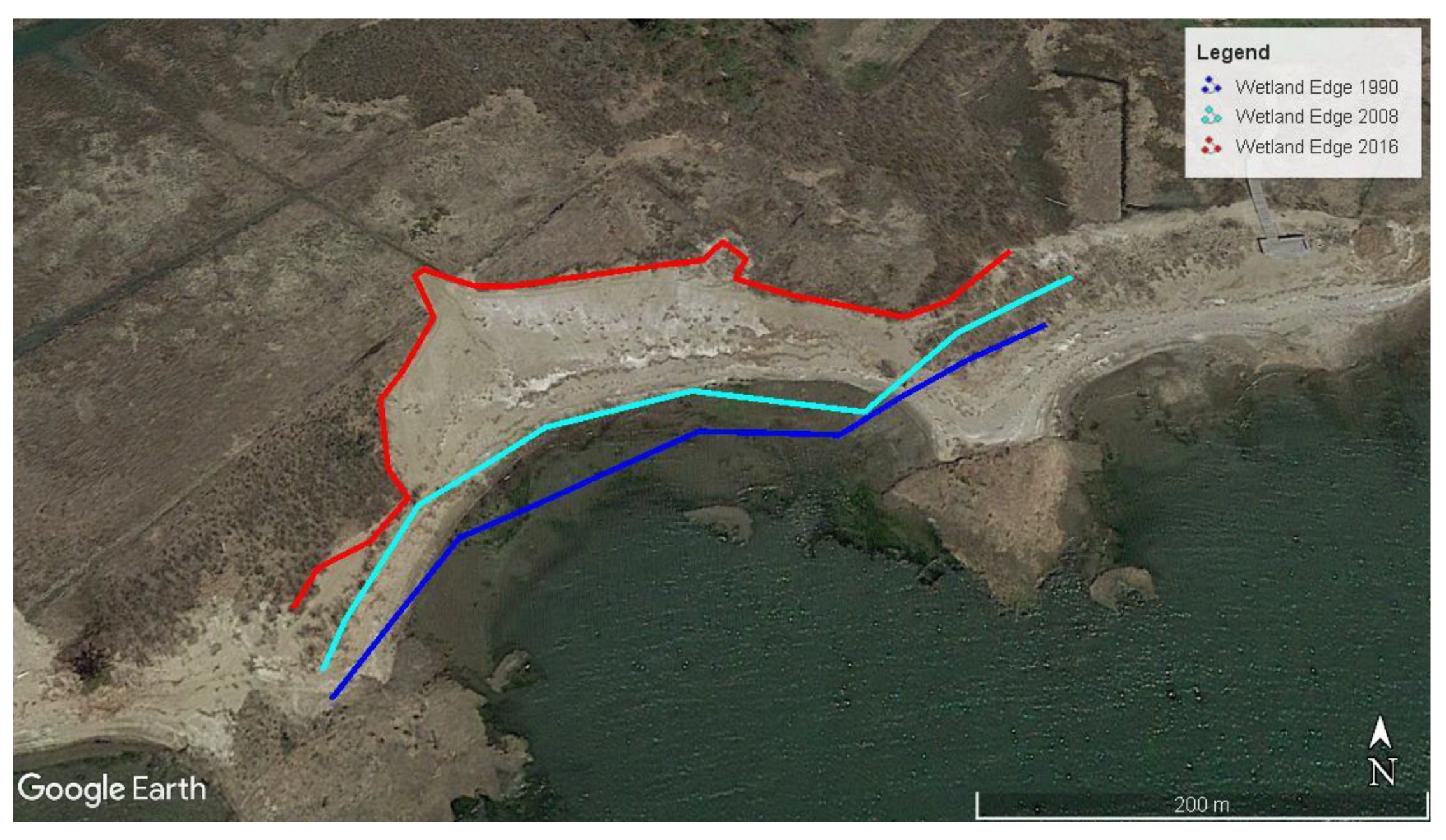
Figure 21.
Reef balls can be used for attenuating wave instead of breakwater.
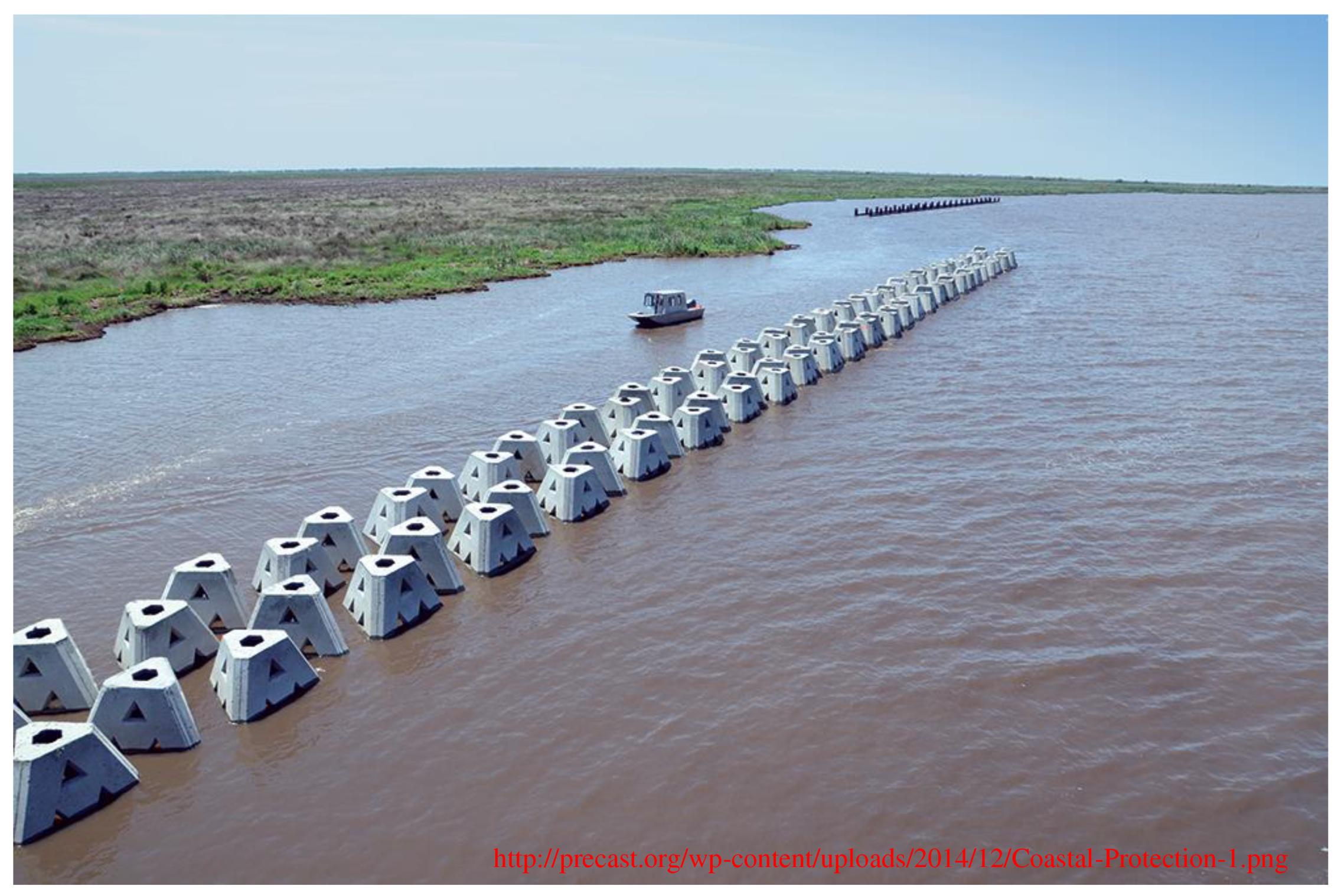
Figure 22.
Proposed resilience plan for protecting the coastline, Yellow lines: reef balls, Green polygon: salt marsh. This is just a fundamental plan. To have a sustainable and resilient protection system and ensure accretion rates of salt marsh, a comprehensive study should be done on sediment supply from West River and circulation in the coastline. The system should be able to accumulate sediment supplies from the West River.
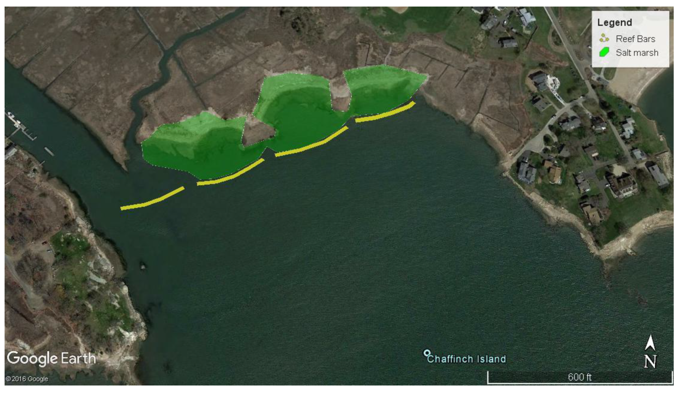
Figure 23.
Short beach situation in the coats of Stratford in Connecticut, the coastline is surrounded by headland in south and Housatonic River in North. Fetch length is strongly restricted in the area and the maximum fetch length is about 2 km from North (red Line). Tidal and river currents are the primary sources of energy in the coastline.
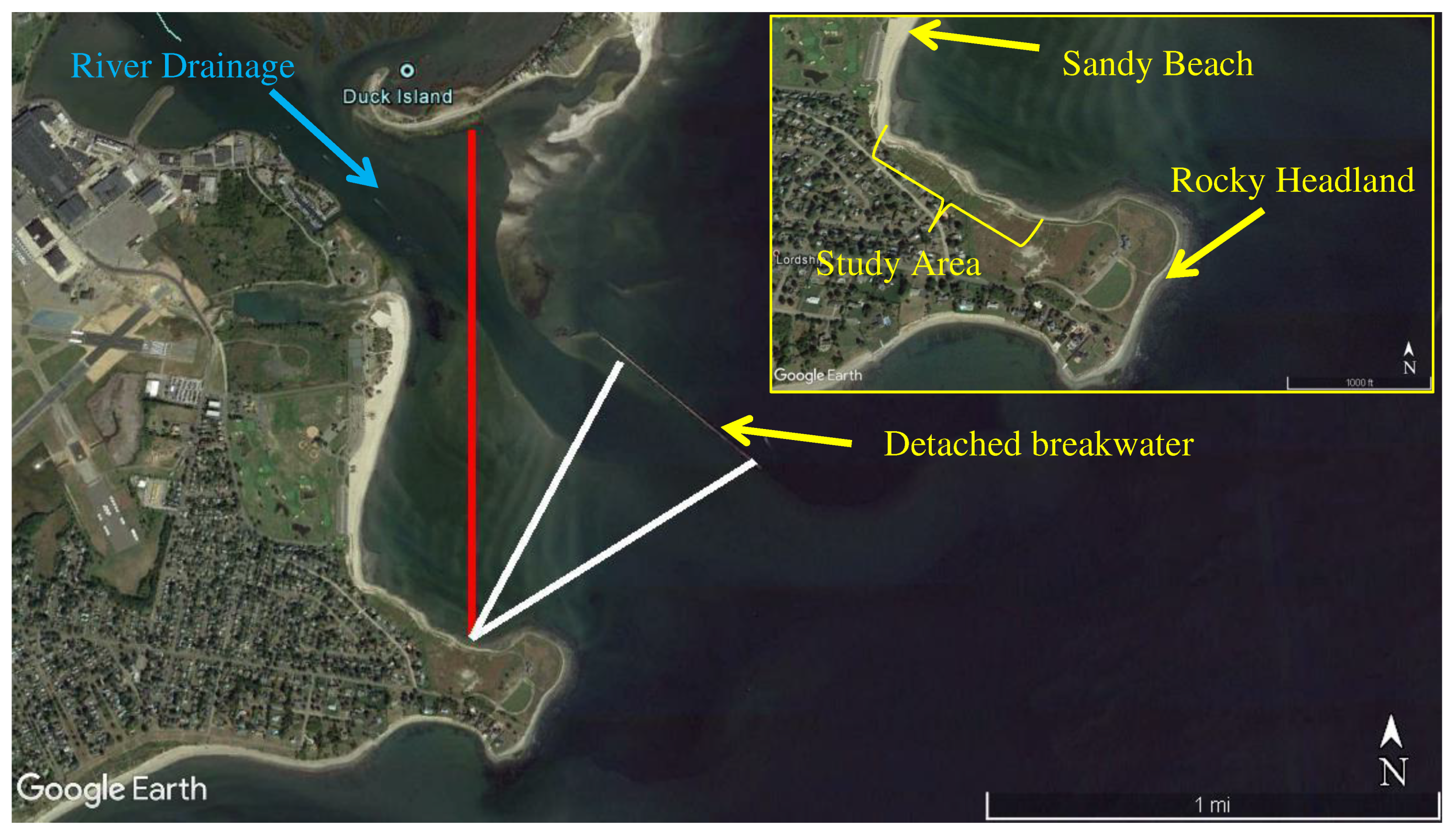
Figure 24.
Comparison of coastal variations between 04/11/1991 and 09/22/2015 (14 years) in Short beach, top left: 1991 image, top right: 2015 image, bottom: the comparison of two coastlines. About 2700 m2 (29000 ft2) of the coastline and 5000 m2 (54000 ft2) of the headland has been eroded in 14 years. However, there is small sedimentation at the northern part.
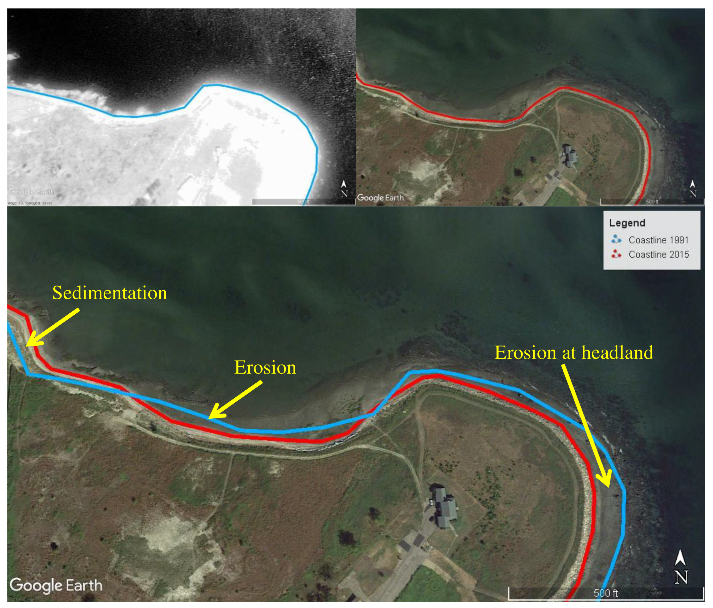
Figure 25.
Ecological-based coastal protection system in Short Beach. Since setting up the protection system, sediment erosion has stopped and the system successfully trapped sand and finer sediment.
Figure 25.
Ecological-based coastal protection system in Short Beach. Since setting up the protection system, sediment erosion has stopped and the system successfully trapped sand and finer sediment.
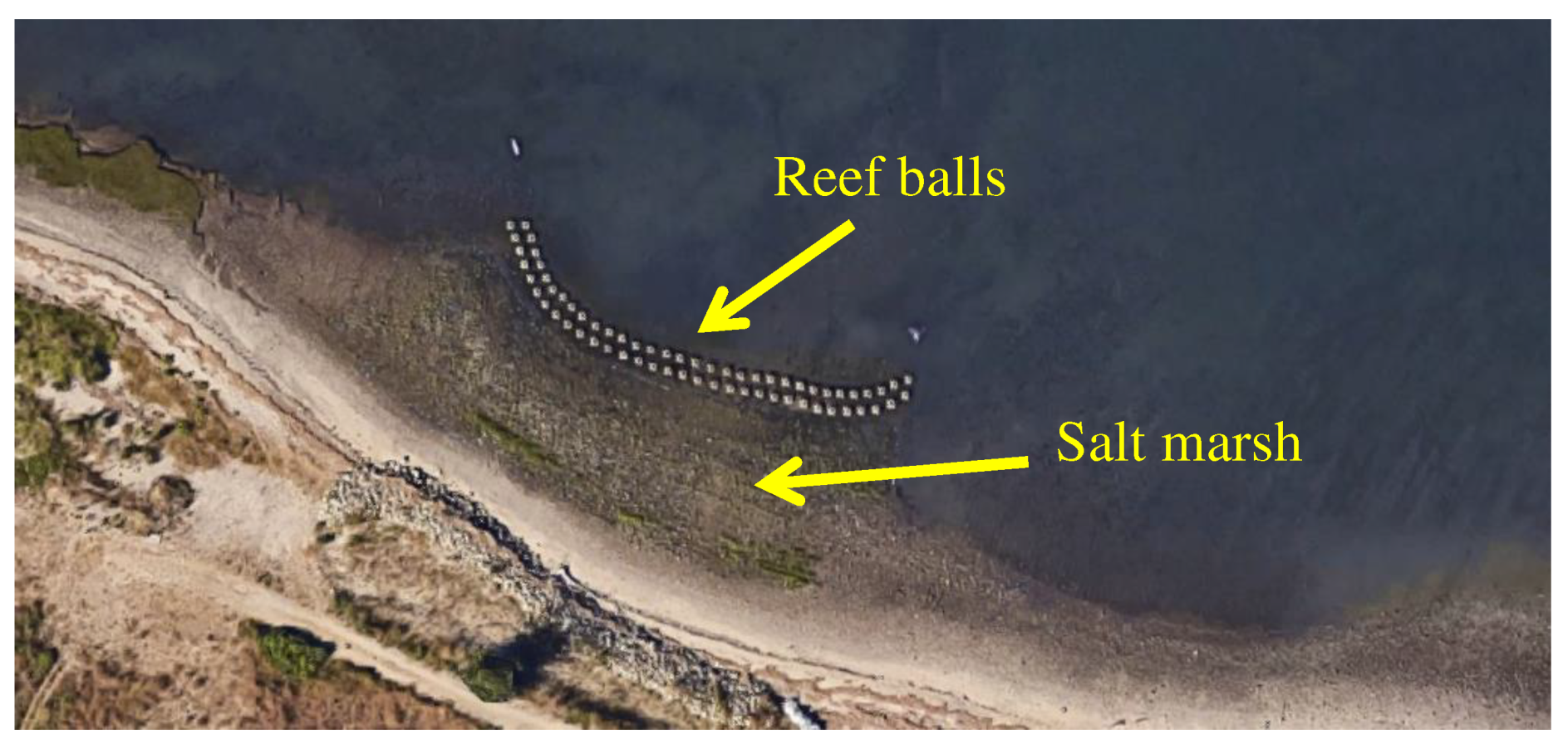
Table 1.
Strengths and weaknesses of protection systems by type, (Sutton et al., 2015).
| Structure type | Strength | Weakness |
|---|---|---|
| Built (seawalls, levees, bulkheads, etc.) |
|
|
| Natural (salt marsh, mangrove, beach, dune, oyster and coral reefs, etc.) |
|
|
| Hybrid (combination of built and natural) |
|
|
Table 2.
Data source of historic, intermediate, and present-day estimates of wetland 22.
| Year(s) | Connecticut Data Sources | New York Data Sources |
|---|---|---|
| 1880s | National Oceanic and Atmospheric Administration (NOAA) Topographic Survey Sheets (T-Sheets), 1880 – 1890s | NOAA Topographic Survey Sheets (T-Sheets), 1880 – 1890s |
| 1970s | Connecticut Department of Energy and Environmental Protection (CT DEEP) 1970s Tidal Wetlands | New York State Department of Environmental Conservation (NYSDEC) 1974 Tidal Wetlands Map |
| 2000s | National Wetlands Inventory (NWI) 2010-2012 | National Wetlands Inventory (NWI) 2004-2009 |
Table 3.
Revised tidal wetland acreage values (Basso et al., 2015).
| 1880s | 1970s | 2000s | |
|---|---|---|---|
| CT | 19,828 | 13,443 | 14,566 |
| NY | 5,342 | 3,464 | 2,790 |
| LIS Total | 25,170 | 16,907 | 17,356 |
Table 4.
Percentage change in wetlands in Long Island Sound (Basso et al., 2015).
| 1880s-1970s | 1970s-2000s | 1880s-2000s | ||||
|---|---|---|---|---|---|---|
| Change (Acres) | Change (%) | Change (Acres) | Change (%) | Change (Acres) | Change (%) | |
| CT | -6,385 | -32% | 1,123 | 8% | -5,262 | -27% |
| NY | -1,878 | -35% | -674 | -19% | -2,552 | -48% |
| LIS Total | -8,263 | -33% | 449 | 3% | -7,814 | -31% |
Table 5.
Marshes Open water scores by location in Long Island Sound (Basso et al., 2015).
| Basin | Tidal wetland acres | Open water acres | % open water at low tide |
|---|---|---|---|
| Western | 345 | 113 | 33% |
| Central | 1,394 | 684 | 49% |
| Eastern | 2,821 | 1,628 | 58% |
1 The current version of this review paper was done originally in Spring 2017 and does not reflect any later study. |
Disclaimer/Publisher’s Note: The statements, opinions and data contained in all publications are solely those of the individual author(s) and contributor(s) and not of MDPI and/or the editor(s). MDPI and/or the editor(s) disclaim responsibility for any injury to people or property resulting from any ideas, methods, instructions or products referred to in the content. |
© 2023 by the author. Licensee MDPI, Basel, Switzerland. This article is an open access article distributed under the terms and conditions of the Creative Commons Attribution (CC BY) license (https://creativecommons.org/licenses/by/4.0/).
Copyright: This open access article is published under a Creative Commons CC BY 4.0 license, which permit the free download, distribution, and reuse, provided that the author and preprint are cited in any reuse.


