
Submitted:
17 November 2026
Posted:
18 November 2026
You are already at the latest version
Abstract
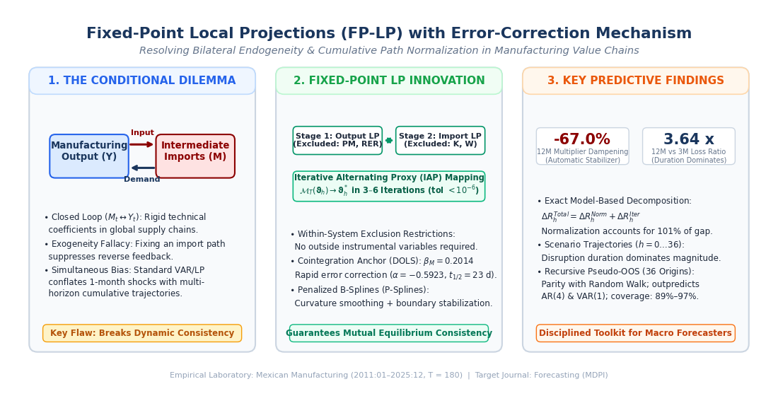
When economic variables operate in a closed loop of bilateral feedback (\(M_t \leftrightarrow Y_t\)), conditional forecasting encounters a fundamental methodological dilemma. Imposing an externally specified future trajectory on one endogenous variable while allowing the second to respond alters the first variable through reverse feedback, breaking dynamic consistency. Conversely, treating the conditioning path as an exogenous driver throughout the forecast horizon suppresses the reverse feedback channel and conflates direct impulse transmission with cumulative system-wide interaction. This paper develops an Iterative Alternating Proxy (IAP) computational framework—Fixed-Point Local Projections (FP-LP) with an Error-Correction Mechanism (ECM)—for conditional forecasting and model-based scenario analysis under bilateral feedback, without claiming closed-form structural identification or new asymptotic distribution theory for the over-identified Huber-IAP estimator. At each horizon h, the procedure embeds two-equation local projections within an alternating Gauss–Seidel updating loop, iteratively re-estimating generated fitted proxies until mutual numerical consistency is attained conditional on maintained within-system exclusion restrictions. Crucially, the methodology yields an exact model-based three-way response decomposition (\(R_h^{FP} = R_h^{SP} + \Delta R_h^{Norm} + \Delta R_h^{Iter}\)) that separates the converged cumulative fixed-point trajectory from a restricted single-pass impulse benchmark (\(R_h^{SP}\)) into a cumulative proxy normalization shift (\(\Delta R_h^{Norm}\)) and iterative feedback updating (\(\Delta R_h^{Iter}\)). Deploying the Mexican manufacturing sector (2011:01–2025:12) as an empirical application, the decomposition shows that the 66.9% reduction at h=12 relative to the single-pass impulse projection is primarily a normalization shift from one-month impulse scaling to cumulative import-path scaling (\(\Delta R_{12}^{Norm} = -0.6924\)), whereas iterative feedback updating (\(\Delta R_{12}^{Iter} = +0.0069\), peaking at +0.0664 at \(h=21\)) contributes much less. At long horizons (h>24), raw local projection estimates become noisy (\(\hat{\gamma}_{1,36} = -0.7923, \text{SE} = 1.385\)), so the FP-SLP terminal trajectory (+0.2004 at h=36, versus −0.4617 without boundary penalties) reflects an imposed DOLS long-run boundary condition (\(\theta_M^{LR} = 0.2014\)) rather than empirically discovered convergence. In the 36-month scenario exercise (which extends beyond the 12-month out-of-sample validation horizon), a 12-month import restriction generates cumulative output losses 3.64 times those of a 3-month restriction of the same monthly magnitude; because a static constant-multiplier benchmark already produces a mechanical ratio of 3.50, the additional +0.14 difference is small and does not constitute strong evidence of dynamic amplification, while absolute cumulative losses remain sensitive to sample period and cointegration rank. Finally, recursive out-of-sample evaluation across 36 holdout origins at horizons of 1, 3, 6, and 12 months detects no statistically significant differences in expected squared-error loss relative to the naive random walk benchmark.
Keywords:
fixed-point local projections
; bilateral endogeneity
; conditional forecasting
; dynamic response decomposition
; feedback effect
; error-correction model
; Mexican manufacturing
; global value chains
1. Introduction
The effect of intermediate imports on output growth in developing countries has proven to be bidirectional. On the one hand, intermediate inputs (M) relax short-run technical constraints and incorporate foreign technological capabilities, enabling output growth trajectories that exceed those attainable solely under the domestic production possibility frontier [1,2,3]. On the other hand, an expansion in manufacturing activity induces higher demand for intermediate inputs due to rigid input-output technical coefficients [4]. This contemporaneous and intertemporal bidirectional feedback () prevents assuming the exogeneity of imports when forecasting GDP behavior in response to changes or restrictions in imports, making it necessary to develop econometric models that reflect such structural endogeneity.
Existing models such as input-output frameworks capture intersectoral dependencies through static accounting schemes that clarify productive structures but cannot be applied to dynamic forecasting [5]. Meanwhile, the plant-level microeconomic literature [1,3,6] estimates gains in total factor productivity while omitting aggregate macroeconomic propagation mechanisms. Macroeconomic balance-of-payments analyses [7,8,9,10,11] establish causality between M and Y by restricting imports to derived demand (), without considering their essential role as a required input for production [1,12]. Finally, standard Vector Autoregression (VAR) models typically impose recursive schemes such as the Cholesky decomposition [13,14,15] and omit long-run cointegration relationships, which can generate simultaneity bias when projecting across intermediate horizons [16,17,18,19,20].
In light of these analytical limitations, the Mexican manufacturing economy serves as an empirical laboratory that enables estimating the effects of bidirectional causality. Mexico’s insertion into North American value chains is distinguished by deep productive integration and sequential production stages [21,22]: imported content exceeds 65% in processing regimes and surpasses 85% in medium- and high-technology industries such as electronics and automotive assembly [23,24,25]. Romero and Aliphat [11] document the existence of structural rigidity in intermediate goods demand functions. From a global perspective, disruptive events—such as the 2011 Tohoku earthquake or the COVID-19 sanitary crisis—have highlighted the acute dependence of local economies on their imports, demonstrating their systemic nature within the domestic productive structure [26,27,28,29].
With the objective of forecasting the bidirectional relationship , this article implements a Fixed-Point Local Projections (FP-LP) computational framework with an Error-Correction Mechanism (ECM) for conditional forecasting and model-based scenario analysis. Inspired by the classical tradition of interdependent systems [30,31,32,33] and contemporary iterative fixed-point algorithms [34,35], the method operationalizes horizon-by-horizon conditional projections under bilateral feedback via an Iterative Alternating Proxy (IAP) regression scheme structured after the Gauss–Seidel updating rule [36,37]. Rather than claiming a fully established structural identification or asymptotic inference theory, or relying on outside instrumental variables external to the macroeconomic system, the procedure imposes maintained within-system exclusion restrictions and iteratively updates the fitted proxy vectors of both equations until converging to a mutually consistent sample fixed point. This computational structure allows us to construct an exact model-based response decomposition comparing the converged cumulative fixed-point projection against a restricted single-pass impulse benchmark, and to generate reproducible conditional forecasts of Mexican manufacturing output under alternative multi-period import trajectories.
The remainder of this article is organized as follows: Section 2 describes the fixed-point methodology and the Iterative Alternating Proxy algorithm; Section 3 details the Mexican manufacturing dataset and long-run cointegration diagnostics; Section 4 presents the model-based response decomposition; Section 5 evaluates four prospective scenarios; Section 6 analyzes recursive out-of-sample predictive validation; Section 7 synthesizes the robustness checks; Section 8 discusses methodological and economic policy implications; and Section 9 concludes.
2. The Bilateral Feedback Problem and Fixed-Point Methodology
2.1. The Bilateral Dynamic System
Building on Yamaguchi [33], the underlying bilateral dynamic system considers as the core vector of dynamically endogenous variables at time , where denotes manufacturing output and denotes intermediate imports:
where captures contemporaneous bilateral feedback:
The parameter represents the conditional projection coefficient (proxy-based output multiplier) of manufacturing output with respect to imported intermediate inputs (), while represents the conditional projection coefficient (proxy-based import multiplier) of intermediate imports with respect to manufacturing output (). denotes the vector of predetermined covariates. When projecting directly across multi-step horizons via Jordà [20] local projections, the cumulative forward changes and (with at ) are conditioned directly on the time-t state vector without requiring iterative multi-step VAR lag inversion ( additional autoregressive differences in the baseline direct projection; see Appendix A.1).
The term defines the error-correction mechanism anchored to the selected long-run empirical production relationship:
Solving for and following simultaneous-equations specification principles [38], the long-run level relation is expressed as:
where includes physical production factors such as capital accumulation and real wages (). In the short-run dynamic local projections, the estimating equations for the bilateral conditional projection coefficients () rely on maintained within-system exclusion and timing assumptions: the output equation includes domestic factor growth () while excluding relative import prices and exchange rate movements (), which enter the import equation alongside U.S. industrial production (, Mexico’s primary export destination). Both equations also include pandemic regime controls: (an indicator equal to 1 during the acute lockdown phase 2020:03–2020:06 and 0 otherwise) and (a post-lockdown regime shift indicator equal to 1 for and 0 otherwise). Importantly, with monthly observations, the excluded covariates and are dated at month t and enter the time-t conditioning information set . Treating them as predetermined particularly at the contemporaneous horizon () rests on the maintained monthly timing assumption that dollar import price indices and exchange rate movements shift within-month import costs before altering domestic physical production technics, while monthly machinery investment and contractual manufacturing wage bills reflect pre-committed domestic factor schedules within the month prior to customs reorder adjustments. As detailed in Appendix A.3, these exclusions and timing conditions are maintained economic modeling assumptions rather than empirically proven quasi-experimental instruments, and because each equation excludes two predetermined covariates (), the alternating proxy algorithm defines an over-identified Iterative Alternating Proxy (IAP) M-estimator rather than a standard Two-Stage Least Squares (2SLS) projection. Table 1 summarizes this specification structure across both stages.
2.2. The Conditional Forecasting Problem and Scenario Convolution Bridge Under Bilateral Feedback
In the presence of bilateral feedback, the traditional empirical literature faces a fundamental dilemma [39,40,41]: (1) If is enforced and is projected in a single stage (via OLS or conventional local projections), it implicitly imposes , ignoring that a drop in manufacturing output contracts derived input demand; (2) If is allowed to respond freely to the trajectory of , the imposed path is distorted and control over the simulated exogenous condition is lost.
The fixed-point procedure addresses this tension computationally by solving for the fitted proxy pair that is mutually consistent across both local projection equations at each horizon h. Conditional scenarios are specified through deviations in the monthly log growth of intermediate imports relative to a common baseline. Let , where denotes intermediate imports, and let denote the first month of the scenario. For scenario s, the monthly perturbation is defined as
where and superscript 0 identifies the baseline path. The values of are prescribed by the assumptions of each scenario. Assuming that the scenario and baseline paths share the same import level in month , the corresponding deviation in log import levels at horizon h is
2.2.1. Linking Cumulative Local Projections to Multi-Period Scenario Paths: Identifying Assumption and Sensitivity
A central methodological question is how horizon-by-horizon cumulative local projection coefficients relate to multi-period scenario simulations. In Stage 1 of the IAP procedure (Equation 6), the estimated equation projects cumulative forward output change onto the converged -month cumulative import proxy . Because the regressor in Equation (6) is itself the -period cumulative import change rather than an isolated period-t innovation , mapping the estimated sequence into a conditional forecast for an arbitrary multi-period sequence of monthly import growth perturbations admits two distinct operational rules:
- Impulse-Translation Convolution Rule (Baseline): If we adopt the impulse-translation approximation—treating as the cumulative output response k months after an isolated permanent shift in the log level of imports of size introduced in month (so that when subsequent growth perturbations are zero)—then defining the implied marginal monthly weights and () yields . Under linear superposition of sequential monthly growth perturbations , the cumulative output deviation at horizon h is given by the discrete convolution:
- Direct Cumulative Window Rule (Sensitivity Alternative): If is instead read literally as the direct projection coefficient multiplying the cumulative log-import deviation accumulated over the window , the implied path is simply , without convolving lagged multipliers across .
Notice that the two rules coincide exactly for a single one-month perturbation ( for ), where and both yield , whereas for multi-month shock paths () the convolution rule weights each monthly innovation by the elapsed horizon . Rather than claiming that these two readings are algebraically identical by identity, we evaluate both rules empirically in Section 5 (Table 5b). Across our 36-month horizon, the baseline convolution rule and the direct window reading produce nearly identical cumulative losses: vs. %-m in Scenario A (trough at vs. at ), vs. %-m in Scenario B (trough at vs. at ), and a Scenario B/A cumulative loss ratio of vs. . Table 7 also verifies exact proportional scaling of the linear convolution code (doubling the monthly perturbation from to scales cumulative output loss by a factor of ), which represents an algebraic property of the linear convolution operator rather than independent empirical evidence of structural linearity.
2.3. Iterative Alternating Proxy Algorithm (Gauss–Seidel Core)
For each prospective horizon on the horizon-trimmed sample of length , we explicitly distinguish the sample IAP fixed point, which solves the finite-sample alternating regression system , from the population fixed-point conditions formalized in Appendix A.3. Importantly, this paper does not establish general consistency or asymptotic normality theorems for the over-identified Huber-IAP estimator, and post-convergence Andrews [42] HAC standard errors are computed conditional on the converged design matrix for use as P-spline precision weights rather than closed-form asymptotic sandwich standard errors. Specifically, the sample algorithm executes through the following stages (written in sample-matrix notation in Appendix A.1):
- Initialization (): In the baseline specification, the initial import proxy vector () is computed on the -observation horizon sample as the fitted values from a Stage-0 Huber M-estimation projection of contemporaneous import growth onto the Stage-2 predetermined controls . Initializing instead with the full union of predetermined controls , the zero vector , or random perturbations yields the exact same converged fixed point to within to , whereas initializing at the orthogonal Stage-0 residual vector (CF Shock) alters initial Huber IRLS robustness weights and steers several horizons into an alternative local M-estimation basin (see Section 7 and Table A1 in Appendix A.4).
- Stage 1 (Output Equation): Using the centered import proxy from the previous iteration, the -winsorized cumulative variation in manufacturing output is projected onto the import proxy and centered Stage-1 predetermined controls via Huber M-estimation:
- Stage 2 (Import Equation): The newly updated manufacturing output fitted proxy () is centered and immediately substituted into the intermediate import equation to re-estimate -winsorized cumulative import variation conditional on centered Stage-2 predetermined controls :
- Stopping Criterion: The alternating regression cycle () repeats until the sum of absolute variations between two successive iterations satisfies the numerical convergence threshold:
In our empirical implementation, the alternating Huber M-estimation algorithm converges in 3 to 6 iterations across all 37 horizons (), with terminal scalar parameter changes between and and full parameter-vector and proxy-vector changes below (see Appendix A.1 and A.2). First-stage relevance diagnostics (detailed in Appendix A.3) confirm that over the primary forecasting horizons , the excluded predetermined price/exchange-rate covariates enter the import equation with joint F-statistics ranging from ( at ) to ( at ), averaging ( at all 13 horizons), while the excluded factor covariates enter the output equation with joint F-statistics up to () and (), averaging across (with weaker relevance at three transition horizons , and attenuating at long horizons for imports). Importantly, we distinguish the sample convergence of this alternating generated-proxy regression operator from the spectral radius of a fixed-coefficient linear simultaneous system (Proposition A1 in Appendix A.2). While the post-estimation product is below unity for 36 of the 37 horizons (equals at ), that product measures implied linear coupling rather than the contraction modulus of the sample IAP regression operator, which is why the empirical algorithm converges in 4 iterations () even at . Following horizon-by-horizon estimation, cubic P-spline regularization (FP-SLP) with explicit terminal slope, curvature, and level penalties smooths high-frequency sampling fluctuations and stabilizes the 36-month trajectory via a shared terminal boundary anchor (see Appendix D.1).
2.4. Model-Based Three-Way Response Decomposition
From the system expressed in Equations (6)–(7), the difference between the converged fixed-point response and the single-pass impulse benchmark can be decomposed into an exact additive identity that separates the normalization change from iterative feedback adjustments. We define three operational quantities at each horizon h:
- Single-Pass Impulse Benchmark (): Represents the P-spline smoothed output projection obtained when the Stage-2 iterative feedback loop is shut down () and cumulative output variation is regressed in a single pass on the initial Stage-0 one-period import proxy and Stage-1 controls :
This benchmark captures the standard dynamic multiplier of output with respect to an isolated, single-month import innovation ( at ).
- Cumulative-Proxy Single-Pass Benchmark (): Represents the projection of cumulative output variation onto the un-updated -month cumulative Stage-0 import proxy , holding the Stage-2 feedback channel shut down ():
This intermediate benchmark measures the output elasticity with respect to an -month cumulative sequence of import shocks in the absence of reverse feedback ( at ).
- Total Fixed-Point Response (): Corresponds to the P-spline smoothed multiplier of the fully coupled alternating system (), where is projected onto the iteratively converged cumulative import proxy and Stage-1 controls :
reaching at and peaking at at .
2.4.1. Exact Additive Identity
The total model-based response gap satisfies the exact additive decomposition:
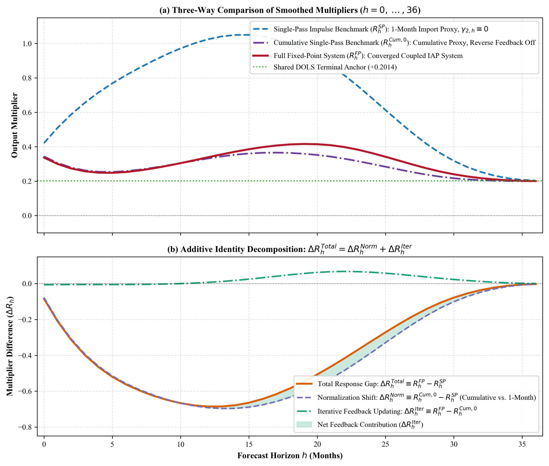
As established in Section 4 and Appendix A.6, at horizon , the total gap is . The normalization shift accounts for 101.0% of the observed dampening, whereas iterative feedback updating contributes (reaches to at ). This demonstrates algebraically that the 66.9% divergence between specifications at is overwhelmingly a normalization shift between an impulse response to a single transient shock versus an elasticity with respect to cumulative import volume, while the iterative Gauss–Seidel feedback adjustment is comparatively modest ( at and up to at , so the single-pass cumulative-proxy estimator already approximates the first-order level of the full FP-SLP curve). We report both the net-scaled response share and the bounded direct-attenuation ratio .
The methodological framework supports two complementary modalities: FP-LP (Fixed-Point Local Projections), which estimates coefficients point-by-point and independently for each horizon and is employed in our out-of-sample predictive evaluation; and FP-SLP (Fixed-Point Smooth Local Projections), which applies a cubic P-spline penalty [43,44] to regularize impulse response curves and scenario convolutions.
3. Data and Transformations
3.1. Data Description
Model estimation utilizes standardized native monthly data for the Mexican economy covering the uninterrupted period 2011:01–2025:12 ( monthly observations, retrieved in January 2026). All seven source series are compiled directly at native monthly calendar frequency—requiring zero temporal interpolation, frequency disaggregation, or series splicing—and are re-indexed to a common reference base year (by dividing each monthly level series by its 2018:01–2018:12 twelve-month arithmetic mean and multiplying by 100) prior to taking natural logarithms in non-seasonally adjusted levels (see Table 2):
- : Manufacturing Production Physical Volume Index (INEGI, Encuesta Mensual de la Industria Manufacturera, EMIM, total manufacturing sector NAICS 31–33, native base ).
- : Real Intermediate Goods Imports Volume Index (, constructed by deflating nominal monthly intermediate goods imports in thousands of U.S. dollars from Banco de México SIE Series SE35401 by the U.S.-dollar Import Price Index , SIE Series SP12755, and re-indexing to ).
- : Monthly Gross Fixed Capital Formation Physical Volume Index in Total Machinery and Equipment (INEGI, Indicador Mensual de la Formación Bruta de Capital Fijo, IMFBCF, Row 77, native base , serving as the high-frequency physical capital accumulation proxy).
- : Real Manufacturing Wage Bill Index (, constructed by deflating nominal monthly total manufacturing remuneration in thousands of Mexican pesos from INEGI EMIM by the headline National Consumer Price Index, INEGI INPC / Banco de México SIE Series SP1 with native base re-referenced to , and re-indexing the resulting real wage bill to ).
- : Import Price Index in U.S. Dollars (Banco de México SIE Series SP12755, re-indexed to base ).
- External Controls: U.S. Industrial Production Index (, Board of Governors of the Federal Reserve System / FRED Series INDPRO, native base , re-indexed to ) and Broad Real Effective Exchange Rate Index for Mexico (, Bank for International Settlements / Banco de México, CPI-deflated trade-weighted index, native base , re-indexed to ).
Unit root and stationarity diagnostics—Augmented Dickey–Fuller [45], Phillips–Perron [46], and KPSS [47]—confirm that the system series behave as processes in levels and are stationary in first differences (see Appendix B.1 for detailed statistics and discussion of borderline trend-stationarity in and ).
3.2. Long-Run Productive Specification and Cointegration
The Johansen [48] multivariate cointegration test on the four-variable system identifies two statistically significant cointegrating relationships ( at ; at ; at ). In the estimated Rank-2 VECM (see Appendix A.3), the output equation loads significantly on the first cointegrating relation () and does not reject weak exogeneity with respect to the second (, Wald ), whereas the import equation loads significantly on the second relation (). Accordingly, our baseline conditions on a single long-run empirical production specification normalized on manufacturing output [48,49], while we explicitly report the sensitivity to including both Johansen cointegrating vectors ( and ) in both stages in Section 5 (Table 5b and Appendix A.3), where absolute cumulative losses expand under Two-ECT while the relative Scenario B/A ratio remains unchanged. We estimate the selected long-run production relation via Dynamic Ordinary Least Squares (DOLS) [50] with one lead and lag () and Andrews [42] HAC correction:

Table 3.
Selected DOLS Long-Run Production Relation and Error-Correction Adjustment.
| Parameter | Regressor | Coefficient | HAC Standard Error | t-Statistic | p-Value |
|---|---|---|---|---|---|
| Intermediate Inputs () | |||||
| Machinery Investment () | |||||
| Real Wage Bill () | |||||
| Intercept | |||||
| Error Correction () |
Notes: Formal system cointegration rank () is established by the multivariate Johansen Trace and Max-Eigenvalue tests (; see Table B2). The univariate ADF statistic on the single-equation DOLS residual is (univariate ), which does not independently reject the Phillips–Ouliaris [51] four-variable residual no-cointegration null at the 5% level (critical value ); accordingly, we rely on the multivariate Johansen test for cointegration support and treat the DOLS vector as a selected empirical equilibrium anchor rather than a uniquely identified structural vector proved by residual testing alone (see Appendix A.3 and B.3). Conditional on , the single-equation conditional LP-ECM adjustment coefficient (; compared to in the four-variable reduced-form VECM that omits contemporaneous import growth and external controls) implies a first-order autoregressive error-correction half-life of months ( days on a 30-day monthly basis). This half-life formula relies on the simplifying assumption of homogeneous first-order AR(1) decay holding predetermined regressors and future shocks fixed at zero, and its rapid adjustment speed is offered as a possible economic interpretation consistent with Just-in-Time inventory management rather than a directly measured firm-level inventory mechanism. Toda–Yamamoto [52] augmented VAR() Granger causality tests () confirm strong reduced-form bidirectionality (: ; : ).
4. Model-Based Response Decomposition in Action: Three-Way Multiplier Analysis
We introduce a standardized negative unit shock to intermediate imports at : () and compare the single-pass impulse benchmark and cumulative-proxy benchmark against the converged fixed-point cumulative response , evaluating the exact additive identity across 36 months:
Table 4.
Empirical Model-Based Three-Way Response Decomposition ().
| Horizon (h) | Single-Pass () | Cumulative () | Fixed-Point () | Normalization () | Feedback () | Total Gap () | Economic Interpretation (Hypothesized Mechanism) |
|---|---|---|---|---|---|---|---|
| 0 (Impact) | Consistent with: Buffering via reserve inventories | ||||||
| 1 | Consistent with: Initial adjustment of factory orders | ||||||
| 3 | Consistent with: Depletion of safety stock | ||||||
| 6 | Consistent with: Derived-demand and cumulative scaling gap | ||||||
| 9 | Consistent with: Ascending phase of single-pass projection | ||||||
| 12 | Consistent with: Maximum model-based response divergence | ||||||
| 15 | Consistent with: Peak of single-pass benchmark () | ||||||
| 18 | Consistent with: Onset of maximum net response phase | ||||||
| 19 | Consistent with: Peak of fixed-point response () | ||||||
| 21 | Consistent with: Derived-demand feedback re-acceleration | ||||||
| 24 | Consistent with: Acceleration of error-correction attraction | ||||||
| 27 | Consistent with: Transition toward terminal anchor | ||||||
| 30 | Consistent with: Narrowing of benchmark gap | ||||||
| 33 | Consistent with: Near terminal alignment | ||||||
| 36 (Long-Run) | Consistent with: Imposed DOLS terminal alignment () |
Notes: is the P-spline regularized single-pass projection of cumulative output change onto the Stage-0 one-period import proxy holding . projects cumulative output onto the -period cumulative Stage-0 proxy holding . is the P-spline regularized fixed-point cumulative multiplier projecting onto the iteratively converged cumulative import proxy . isolates the normalization shift, captures the iterative feedback updating, and . The final column provides narrative economic hypotheses rather than directly tested firm-level channels.
Across all evaluated horizons, the model-based gap takes strictly negative values. Rather than generating explosive amplification, conditioning on the feedback-updated cumulative import trajectory yields substantially more moderate medium-run multipliers than projecting cumulative output directly onto the initial one-month import proxy. Crucially, the three-way decomposition reveals that the 66.9% reduction at ( vs. , ) is driven almost entirely by the normalization shift (, accounting for 101.0% of the difference), reflecting the algebraic transition from evaluating an isolated one-month impulse to an -month cumulative shock path. In contrast, the iterative Gauss–Seidel feedback adjustment contributes much less (, peaking at at ), indicating that iterative updating is not the dominant driver of the response gap and that the single-pass cumulative-proxy estimator already captures the first-order magnitude of the response curve. By month 36 (), both P-spline regularized curves align at the DOLS long-run production elasticity anchor (, , ). We emphasize prominently that this terminal alignment represents an imposed long-run boundary condition rather than empirically discovered convergence: as detailed in Appendix D.1 and Table D2, the raw unsmoothed long-horizon local projection estimates are highly unstable ( with raw HAC standard error , compared to , , and ), and removing the terminal boundary penalties causes the unanchored smoother to terminate at (or under flat-tail derivative penalties alone with ). Consequently, for the FP-SLP trajectory is materially governed by the imposed DOLS equilibrium anchor ( at ) and standard-error capping () rather than independent identification from monthly long-horizon data. Figure 1 and 2 illustrate the FP-SLP dynamic response profile with its conditional bootstrap confidence bands and the three-way model-based decomposition across the 36-month horizon.
Figure 1.
FP-SLP Dynamic Projection Multiplier of Mexican Manufacturing Output to a Standardized Intermediate Import Perturbation. Notes: The horizontal dashed line (+0.2014) indicates the imposed terminal P-spline boundary regularization anchor set equal to the DOLS long-run production coefficient reported in Table 3 (); for , the smoothed trajectory reflects this imposed boundary condition rather than unconstrained monthly sample convergence (raw ; unanchored smoother ). Shaded 95% Moving Block Bootstrap intervals are conditional on the fixed smoothing parameter and terminal anchor .
Figure 1.
FP-SLP Dynamic Projection Multiplier of Mexican Manufacturing Output to a Standardized Intermediate Import Perturbation. Notes: The horizontal dashed line (+0.2014) indicates the imposed terminal P-spline boundary regularization anchor set equal to the DOLS long-run production coefficient reported in Table 3 (); for , the smoothed trajectory reflects this imposed boundary condition rather than unconstrained monthly sample convergence (raw ; unanchored smoother ). Shaded 95% Moving Block Bootstrap intervals are conditional on the fixed smoothing parameter and terminal anchor .
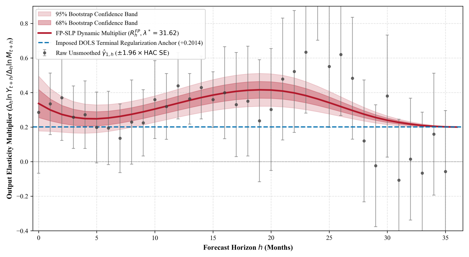
Figure 2.
Model-Implied Dynamic Response Decomposition: Single-Pass Impulse Benchmark (), Cumulative Benchmark (), Total Fixed-Point Response (), and Component Disaggregation.
Figure 2.
Model-Implied Dynamic Response Decomposition: Single-Pass Impulse Benchmark (), Cumulative Benchmark (), Total Fixed-Point Response (), and Component Disaggregation.
5. Conditional Forecasting Scenarios Under Alternative Trajectories
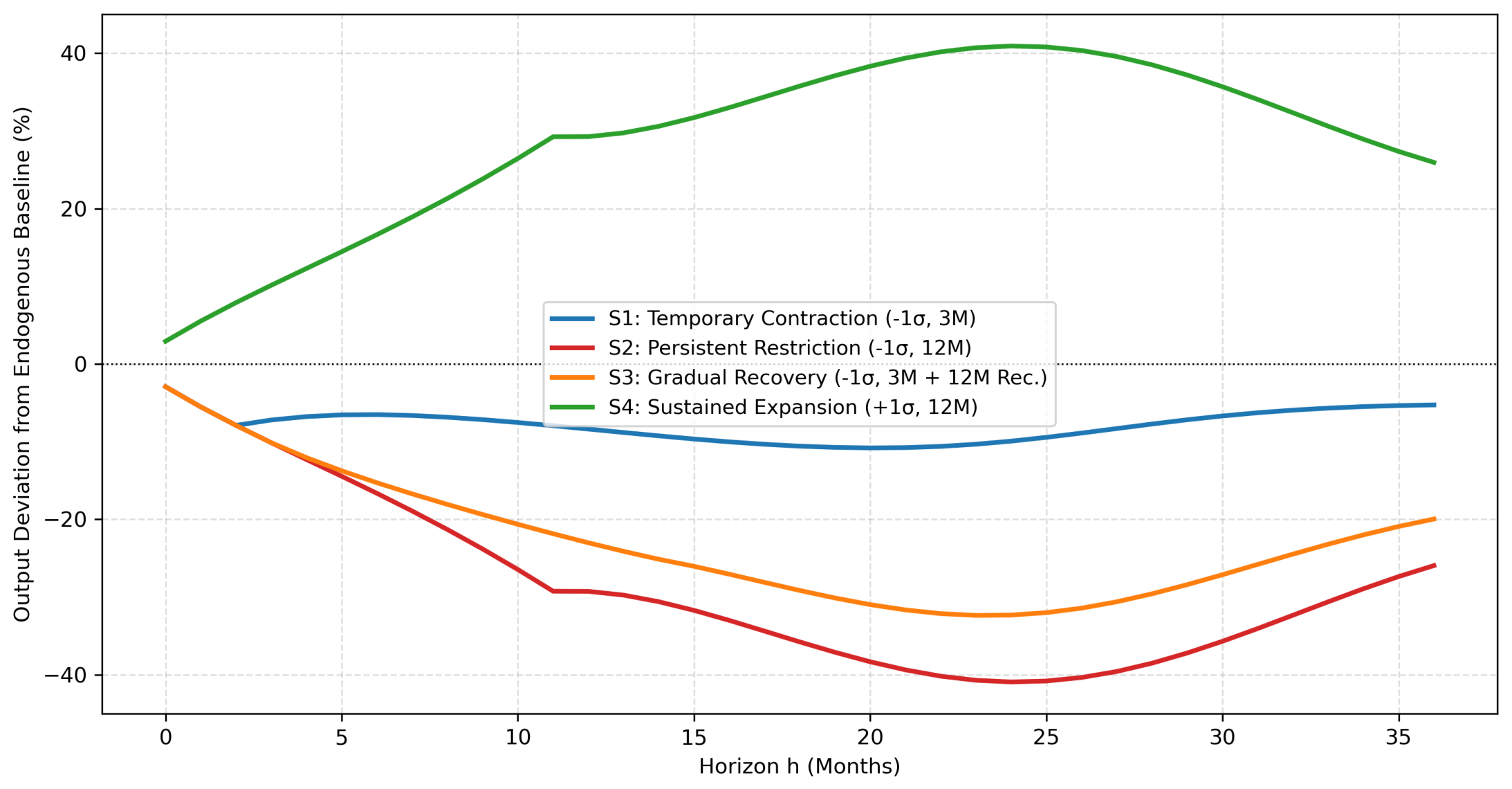
We evaluate four prospective 36-month scenarios by convolving monthly import log-growth deviations from baseline, , with the estimated and smoothed fixed-point multipliers introduced in Section 2:
(analogously for the single-pass benchmark; see Section 2.2 and Appendix A.6). Under the impulse-translation approximation discussed in Section 2.2, an isolated perturbation in monthly log import growth in month (followed by zero subsequent growth deviations) shifts the cumulative log-import level over the remaining elapsed horizon by . For a perturbation introduced in month j, its contribution to the output deviation at horizon h is therefore calculated using the multiplier corresponding to the elapsed horizon , , and we compare this baseline convolution directly against the alternative cumulative window rule in Table 5b:
- Scenario A (Transitory Contraction): A () monthly import growth restriction for 3 months (), followed by thereafter.
- Scenario B (Persistent Restriction): A () monthly import growth restriction sustained continuously for 12 months ().
- Scenario C (Gradual Recovery): A drop for 3 months (), followed by a gradual 12-month linear decay of the growth perturbation back to zero over months .
- Scenario D (Sustained Expansion): A () monthly expansion sustained for 12 months (, associated with supply-chain relocation investments, nearshoring).
Table 5.
Conditional Projections of Manufacturing Output with Draw-by-Draw 95% Bootstrap Confidence Intervals.
Table 5.
Conditional Projections of Manufacturing Output with Draw-by-Draw 95% Bootstrap Confidence Intervals.
| Scenario | Horizon | Shock () | Total FP () | Single-Pass () | Gap () | Basic (Bias-Corr.) 95% CI | Raw Percentile 95% CI |
|---|---|---|---|---|---|---|---|
| A: Transitory | [, ] | [, ] | |||||
| (, 3M) | [, ] | [, ] | |||||
| [, ] | [, ] | ||||||
| (Peak) | [, ] | [, ] | |||||
| [, ] | [, ] | ||||||
| 12M Loss | — | %-m | %-m | %-m | [, ] | [, ] | |
| 36M Loss | — | %-m | %-m | %-m | [, ] | [, ] | |
| B: Persistent | [, ] | [, ] | |||||
| (, 12M) | [, ] | [, ] | |||||
| [, ] | [, ] | ||||||
| (Peak) | [, ] | [, ] | |||||
| [, ] | [, ] | ||||||
| 12M Loss | — | %-m | %-m | %-m | [, ] | [, ] | |
| 36M Loss | — | %-m | %-m | %-m | [, ] | [, ] | |
| C: Gradual | Peak () | — | [, ] | [, ] | |||
| (, 3M+12M Rec.) | 36M Loss | — | %-m | %-m | %-m | [, ] | [, ] |
| D: Expansion | Peak () | — | [, ] | [, ] | |||
| (, 12M) | 36M Gain | — | %-m | %-m | %-m | [, ] | [, ] |
Notes: Cumulative losses are expressed in percentage-point-months (%-m) summed across (37 terms). Confidence intervals are computed directly from Moving Block Bootstrap resamples ( months, valid draws) by convolving the scenario shock paths draw-by-draw with each bootstrap multiplier curve . In each bootstrap replication b, we re-estimate on the resampled block dataset: (i) the DOLS long-run vector , (ii) the resulting error-correction term , (iii) the horizon-by-horizon Huber-IAP fixed point , and (iv) the post-convergence Andrews HAC inverse-variance weights , while holding fixed at their full-sample baseline values (v) the interior smoothing parameter and (vi) the terminal level anchor ; accordingly, the reported bootstrap intervals are conditional on . We report both the basic (bias-corrected pivotal) 95% bootstrap interval and the raw percentile 95% interval . Crucially, for cumulative 12M and 36M losses in all four scenarios—as well as the Scenario B/A 36M loss ratio (, basic 95% CI , raw percentile 95% CI )—the point estimates lie inside both the raw percentile and basic 95% intervals. At individual peak horizons , raw bootstrap percentiles lie closer to zero than the point trough because block resampling of length breaks multi-year post-2020 persistence and attenuates the medium-run multiplier hump toward (bootstrap bias of at and at ).
To evaluate the structural and mechanical drivers of these prospective projections, Table 5b presents a comprehensive nine-specification stress-test comparing both the absolute 36-month cumulative losses and the Scenario B to Scenario A loss ratio. In addition to six econometric specification checks—(1) the baseline full sample, (2) the Rank-2 Johansen two-ECT specification, (3) the seasonally controlled specification with 11 month-of-year dummies, (4) the unanchored flat-tail spline (), (5) the pre-pandemic subsample (2011–2019), and (6) the post-lockdown subsample (2020–2025)—we include three diagnostic benchmarks that isolate the effects of HAC standard-error capping, the scenario convolution rule, and pure shock-window arithmetic: (7) P-spline smoothing weighted by uncapped Andrews HAC standard errors, (8) the direct cumulative window reading, and (9) a constant-multiplier mechanical benchmark ( for all h).
Notes: Cumulative losses are expressed in percentage-point-months (%-m) over (37 horizon terms). Under a constant time-invariant multiplier , a 3-month shock of size accumulates , whereas a 12-month shock accumulates , yielding an exact mechanical baseline ratio of (or over ). Thus, of the baseline ratio reflects the pure horizon arithmetic of sustaining a 12-month vs. 3-month import contraction over a 37-month window, while the remaining () is the small additional difference contributed by the medium-run FP-SLP multiplier hump () relative to the pre-pandemic flat trajectory (, which lies below ).
Three key empirical conclusions emerge from Table 5b. First, regarding the Scenario B/A loss ratio, because a constant-multiplier benchmark () already yields a ratio of purely from shock-duration arithmetic, the additional difference in the baseline ( vs. ) is relatively small and should not be interpreted as strong evidence of nonlinear or dynamic amplification. Second, in contrast to the stability of the relative B/A ratio (), the absolute cumulative scenario losses exhibit substantial sensitivity across specifications and sample periods: Scenario B’s 36-month cumulative loss ranges from %-m (trough ) in the pre-pandemic 2011–2019 subsample to %-m under seasonal adjustment, %-m with uncapped HAC weights, %-m in the baseline, %-m under the Rank-2 Two-ECT specification (trough ), and %-m in the post-lockdown 2020–2025 subsample (trough ). Inspecting the full multiplier profile of the seasonally controlled specification (11 monthly calendar dummies) further clarifies that the medium-run multiplier hump itself survives seasonal adjustment (, , peaking at and vs. in the baseline, with ), whereas the contemporaneous point estimate shifts to () as calendar dummies absorb high-frequency within-year seasonal co-movement. Third, we emphasize that this 36-month scenario exercise is not empirically validated at long horizons by our out-of-sample forecasting evaluation in Section 6 (which evaluates horizons only up to months), and for the scenario trajectories depend directly on the imposed DOLS terminal anchor .
It is also necessary to note that the model-implied response decomposition constitutes a conditional accounting framework rather than a counterfactual causal identification, and that the linear convolution presupposes perturbations within the historical variation range. Figure 3 and 4 display the conditional output trajectories across the four scenarios. Figure 3 provides an in-level historical reconstruction of the manufacturing production index () from 2011:01 through the forecast origin at 2025:12 (), followed by the 36-month prospective projections (2026:01–2028:12) with 95% bootstrap confidence bands (conditional on and ), highlighting the historical benchmark of the April 2020 COVID-19 trough (). Figure 4 provides a direct overlay comparison of the four scenario deviations.
Figure 3.
Conditional Manufacturing Output Forecasts Under Four Alternative Import-Path Scenarios in Levels (Panel View: 2011:01–2028:12).
Figure 3.
Conditional Manufacturing Output Forecasts Under Four Alternative Import-Path Scenarios in Levels (Panel View: 2011:01–2028:12).
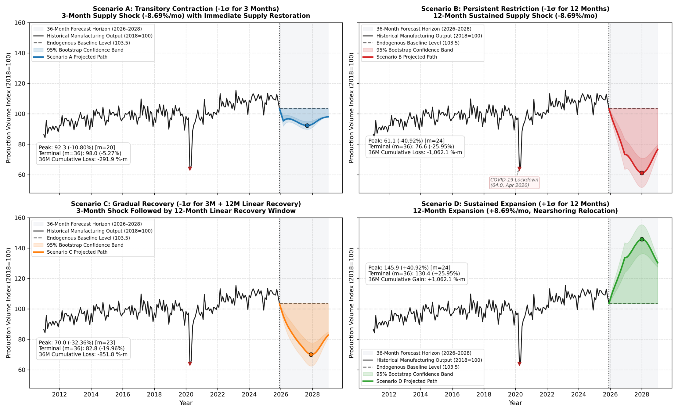
Figure 4.
Overlay Comparison of Conditional Manufacturing Output Forecast Trajectories with 95% Confidence Bands.
Figure 4.
Overlay Comparison of Conditional Manufacturing Output Forecast Trajectories with 95% Confidence Bands.
6. Predictive Validation: Recursive Out-of-Sample Evaluation Across 36 Expanding Windows
To evaluate the out-of-sample predictive performance of the toolkit, we conduct a multi-window recursive pseudo-out-of-sample forecasting exercise designed to assess point accuracy, Diebold–Mariano loss differentials, and empirical prediction interval coverage across historical horizons .
6.1. Recursive Out-of-Sample Accuracy and Coverage Evaluation
Following Clark and McCracken (2013), we conduct an expanding-window recursive evaluation across out-of-sample forecast origins (initial training window through , corresponding to 36 target realizations per horizon across the holdout sample; see Appendix G.1). Crucially, this empirical evaluation covers short-to-medium horizons and 12 months, and therefore does not empirically validate the 36-month scenario projections in Section 5 beyond . Multi-year horizons () cannot be evaluated with non-overlapping recursive windows on a monthly sample of 180 observations without severe sample truncation and overlapping forecast errors; prospective projections for in Section 5 rely instead on semi-parametric P-spline regularization anchored to the imposed long-run DOLS boundary condition.
Table 6 evaluates both the unsmoothed FP-LP ECM and the smoothed FP-SLP ECM estimators against four benchmark models. At , smoothed FP-SLP ECM achieves a point MAE of and a point RMSE of (compared to unsmoothed FP-LP ECM with MAE and RMSE , and Naive Random Walk with MAE and RMSE ), while at the Naive Random Walk achieves lower point MAE () and RMSE (). Importantly, modified Diebold–Mariano / Harvey–Leybourne–Newbold (DM-HLN) tests () do not establish statistically significant predictive superiority of FP-LP or FP-SLP over the random walk at any horizon. Given the limited number of holdout origins () and the serial correlation of overlapping multi-step forecast errors at and 12, the DM-HLN statistics must be interpreted with caution: the evaluation documents the absence of statistically detectable differences in expected squared-error loss relative to the random walk, rather than predictive superiority or equivalence. Analytical 95% prediction intervals constructed from the training-window h-step residual standard deviation achieve empirical coverage of (), (), (), and / ( for FP-LP / FP-SLP), closely tracking the nominal 95% benchmark across the 36 holdout windows.
Notes: Relative MAE (MASE) is the ratio of model MAE to Naive Random Walk MAE ( indicates lower MAE). DM-HLN tests are computed on squared-error differentials (positive values favor the model in RMSE). Empirical 95% coverage reports the percentage of the 36 holdout realizations falling within , where is the expanding training-window h-step residual standard deviation .
6.2. Visual Tracking of Recursive Expanding-Window Forecasts in Reconstructed Index Levels ( and )
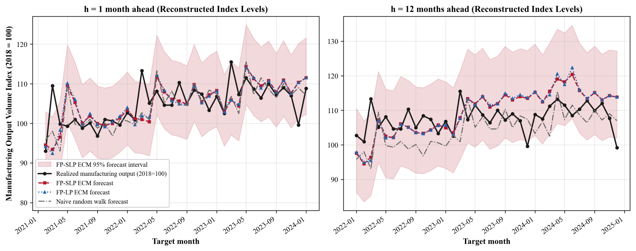
Figure 5 plots the realized trajectory of the Mexican manufacturing production volume index () against the recursive pseudo-out-of-sample level forecasts generated by the smoothed FP-SLP ECM, unsmoothed FP-LP ECM, and Naive Random Walk () models across the 36 expanding evaluation windows at horizons (Panel A, target dates 2021:01–2023:12) and (Panel B, target dates 2021:12–2024:11).
Figure 5.
Recursive Pseudo-Out-of-Sample Forecasts of Mexican Manufacturing Output in Reconstructed Index Levels () Across 36 Expanding Evaluation Windows ( and Months Ahead). Notes: Plotted across 36 expanding windows ( through ) via . Panel A displays 1-month-ahead recursive level forecasts (empirical 95% coverage: 88.9%); Panel B displays 12-month-ahead recursive level forecasts (FP-SLP empirical 95% coverage: 91.7%, log-error RMSE: 0.0607 vs. FP-LP 0.0628 and Naive 0.0650). Shaded bands indicate the 95% expanding-window prediction interval.
Figure 5.
Recursive Pseudo-Out-of-Sample Forecasts of Mexican Manufacturing Output in Reconstructed Index Levels () Across 36 Expanding Evaluation Windows ( and Months Ahead). Notes: Plotted across 36 expanding windows ( through ) via . Panel A displays 1-month-ahead recursive level forecasts (empirical 95% coverage: 88.9%); Panel B displays 12-month-ahead recursive level forecasts (FP-SLP empirical 95% coverage: 91.7%, log-error RMSE: 0.0607 vs. FP-LP 0.0628 and Naive 0.0650). Shaded bands indicate the 95% expanding-window prediction interval.
7. Robustness Analysis
Finally, we conduct a sensitivity and robustness analysis evaluating the behavior of the empirical estimates across eight analytical dimensions (Table 7). The diagnostics confirm that the DOLS long-run elasticities are stable across lead/lag orders and subsample windows, while medium-run local projection multipliers and absolute cumulative scenario losses reflect the higher variance of the 2020–2021 pandemic supply-chain contraction when estimated on the full sample (with Scenario B 36M loss ranging from %-m pre-pandemic to %-m in baseline and %-m under Two-ECT). Furthermore, adding 11 monthly calendar dummies confirms that the medium-run multiplier hump survives seasonal adjustment (, , peaking at and , vs. in the baseline), even though the contemporaneous point estimate shifts to as monthly dummies absorb within-year seasonal co-movement. Comparing FP-SLP against the residual control-function estimator (CF-SLP) shows that while point estimates diverge at intermediate horizons () due to cumulative proxy updating versus single-period residual control, raw Moving Block Bootstrap 95% percentile intervals (conditional on and ) span zero across all 37 horizons (see Appendix F). Lastly, the specifications without and without boundary penalties (Table D2) demonstrate that the error-correction term and the imposed DOLS terminal boundary condition are essential for stabilizing long-horizon trajectories.
Table 7.
Battery of Sensitivity Tests and Robustness Diagnostics.
| Analytical Dimension | Baseline Specification | Alternative Specification | Empirical Result | Conclusion |
|---|---|---|---|---|
| DOLS Lag Structure | () | AIC Selection () | ; DOLS-anchored terminal level () | High parametric stability |
| Estimator Comparison | Alternating Proxy (FP-SLP) | Control Function (CF-SLP) | Impact ( vs. ) and ( vs. ) align at DOLS anchor; raw MBB 95% percentile CIs span 0 at all h, while normal-approx centered CIs exclude 0 at | Point divergence at medium horizons; not decisive under raw MBB percentiles |
| Temporal Stability | Full sample 2011–2025 | Bai–Perron Structural Break Tests & Pre-2020 Subsample | Single break in April 2020 (); pre-pandemic DOLS (); pre-2020 FP-SLP lower at ( at , at ; Scen. B loss vs. %-m) | Stable DOLS vector; higher medium-run response and absolute loss in full sample |
| Seasonal Adjustment | Non-seasonally adjusted + regime controls | Inclusion of 11 month-of-year calendar dummies | shifts to (), while medium-run hump survives (, , peak , , ; B/A ratio ) | Medium-run multiplier hump survives seasonal adjustment |
| Error-Correction & Terminal Anchor | Single ECT + DOLS terminal anchor () | Omitting , Two-ECT (), or unanchored spline () | Without ECT: medium-run downward shift ( at ); Two-ECT: Scen. B loss %-m (ratio ); unanchored spline (): ( flat-tail; Table D2) | Terminal trajectory governed by imposed DOLS boundary condition |
| Initialization Sensitivity | Stage-0 reduced-form init () | Zero vector, , , and orthogonal residual (`CF Shock`) | Convergence in 3–6 steps for zero/union/random starts (); orthogonal residual start (`CF Shock`) alters Huber IRLS weights into alternative basin at some horizons (Table A1) | Invariance within instrument span; IRLS basin sensitivity to residual start |
| Linear Convolution Verification | Base perturbation of | Perturbations scaled to and | Exact proportional scaling: loss at %-m () | Algebraic property of linear convolution calculation (not structural proof) |
| Intertemporal Consistency | Monthly model () | Quarterly aggregation () | Regularized quarterly terminal level aligns with monthly via shared DOLS anchor (; raw , raw ) | Shared boundary regularization across frequencies |
8. Discussion
By structuring estimation horizon-by-horizon via an Iterative Alternating Proxy (IAP) procedure, the FP-LP framework provides a practical computational framework for conditional forecasting and model-based scenario analysis under bilateral feedback, avoiding recursive Cholesky orderings as in traditional VARs [13,14,53] or reliance on outside instrumental variables external to the macroeconomic system that are rarely available at high monthly frequency [33,54,55]. Rather than claiming a fully established structural identification or asymptotic inference method, the procedure operates conditional on maintained within-system exclusion and timing assumptions (Table 1) and the selected long-run error-correction anchor, enabling researchers to impose prospective conditioning paths on intermediate imports while updating endogenous output and import proxies simultaneously across the forecast horizon [39,56,57].
In the Mexican manufacturing application, the model-based three-way decomposition shows that the moderate peak fixed-point projection coefficient ( at , and at ) contrasts sharply with the single-pass projection onto the initial one-month import proxy (, which reaches at and peaks at at ), yielding a negative total response gap (, ). Disaggregating this gap demonstrates that the reduction is overwhelmingly accounted for by the cumulative proxy normalization shift (, or of the gap), whereas the iterative Gauss–Seidel feedback adjustment contributes much less (, peaking at at ) and is not the dominant mechanism. Likewise, at long horizons (), where raw local projection estimates become noisy (), the FP-SLP terminal trajectory () is materially governed by the imposed DOLS long-run anchor () rather than independent identification from monthly data (with the unanchored smoother yielding at ; Table D2). Evidence on input linkages documents the transmission of supply disruptions across firms and countries [26,28]. In our conditional scenarios (which extend to 36 months beyond the 12-month out-of-sample validation horizon), a 12-month import restriction generates cumulative output losses over 36 months that are 3.64 times those generated by a 3-month restriction of the same monthly magnitude (Table 5). Because a static constant-multiplier benchmark already produces a mechanical ratio of (), the additional difference is relatively small and should not be interpreted as strong evidence of dynamic amplification, while absolute cumulative losses vary substantially across subsamples and cointegration specifications (Table 5b). Within this conditional accounting framework, industrial and trade policy analysis can use the scenario convolutions to benchmark the cumulative output exposure associated with persistent supply-chain bottlenecks.
9. Conclusions
This paper develops and applies the Fixed-Point Local Projections (FP-LP) alternating-proxy computational framework to conduct conditional forecasting and model-based scenario analysis in bilaterally coupled time-series systems (). Conditional on maintained within-system exclusion and timing assumptions and a selected error-correction anchor—and without claiming general consistency or asymptotic normality theorems for the over-identified Huber-IAP estimator—the algorithm provides a transparent and reproducible computational method for aligning horizon-by-horizon local projections and decomposing the converged cumulative projection coefficient relative to a restricted single-pass impulse benchmark ().
Applying the framework to Mexican manufacturing across 180 native monthly observations (2011:01–2025:12), we anchor long-run equilibrium adjustments using a DOLS production specification (, alongside multivariate Johansen rank cointegration support) paired with a conditional error-correction term (, implying a first-order AR(1) adjustment half-life of months or days under homogeneous zero-shock decay). The model-based three-way decomposition shows that normalizing by the cumulative import trajectory reduces the projected 12-month multiplier by relative to the single-pass impulse benchmark ( vs. ), with the normalization shift () accounting for nearly the entire difference while iterative feedback updating (, peaking at at ) contributes much less. At long horizons (), raw local projection estimates are unstable (), and the unanchored smoother terminates at ( under flat-tail derivative penalties alone); thus, the FP-SLP endpoint represents an imposed DOLS long-run boundary condition rather than empirically discovered convergence. In the 36-month scenario exercise (which is not validated beyond by the out-of-sample forecasting exercise), a 12-month import restriction generates cumulative output losses 3.64 times those of a 3-month restriction of the same monthly magnitude; because the constant-multiplier benchmark already yields a ratio of , the additional difference is small and does not constitute strong evidence of dynamic amplification, whereas absolute scenario losses vary meaningfully across subsample and Two-ECT specifications ( to %-m in Scenario B). Finally, recursive out-of-sample evaluation across holdout origins at horizons and 12 months evaluates both the unsmoothed FP-LP ECM and smoothed FP-SLP ECM specifications and detects no statistically significant differences in expected squared-error loss relative to the naive random walk benchmark (DM-HLN , interpreted with caution given 36 origins and overlapping multi-step forecast errors), with empirical 95% interval coverage between and . Together, these results offer a disciplined and transparent computational workflow for conditional scenario analysis in interdependent production networks.
Author Contributions
The sole author is responsible for all aspects of this research, including conceptualization, econometric methodology, software implementation, formal validation, empirical analysis, data curation, manuscript preparation, review and editing, and visualization. The author has read and agreed to the published version of the manuscript.
Funding
This research received no external funding.
Institutional Review Board Statement
Not applicable.
Informed Consent Statement
Not applicable.
Data Availability Statement
The complete monthly time-series dataset (2011:01–2025:12, ) compiled from INEGI (EMIM and IMFBCF), Banco de México (SIE Series SE35401, SP12755, and SP1), the Federal Reserve Bank of St. Louis (FRED Series INDPRO), and the Bank for International Settlements (Broad REER), together with the core Python estimator module and the numbered replication pipeline, are included in the supplementary replication archive submitted with this manuscript. To reproduce all tables and figures from a clean Python 3.10+ environment (requiring numpy, pandas, scipy, statsmodels, matplotlib, and pillow), execute the numbered pipeline scripts sequentially from the project root: (1) Step 01 (ETL, data dictionary, and unit-root/Johansen cointegration checks, Tables 2–3 and B1–B2); (2) Steps 02–03 (first-stage relevance F-statistics, operational convergence log, and initialization sensitivity audit, Table A1); (3) Step 05 (GCV surface and 5-specification boundary penalty sensitivity grid, Tables D1–D2); (4) Steps 07–08 (CF-SLP vs. FP-SLP paired block bootstrap comparison and three-way response decomposition, Tables 4, E1, and F1); (5) Step 09 (Rank-2 VECM weak-exogeneity and Two-ECT robustness checks); (6) Steps 15, 17, and 18 (prospective scenario convolutions, mechanical and uncapped-SE stress tests, and draw-by-draw Moving Block Bootstrap intervals, Tables 5 and 5b); (7) Step 16 (36-window recursive out-of-sample evaluation and DM-HLN tests, Tables 6, G1, and G2); and (8) the figure generation and MDPI LATEX/PDF build scripts.
Acknowledgments
The author thanks the anonymous reviewers and the academic editor for their constructive comments and suggestions.
Conflicts of Interest
The author declares no conflicts of interest.
Abbreviations
The following abbreviations are used in this manuscript:
| ADF | Augmented Dickey–Fuller |
| AIC | Akaike Information Criterion |
| CF-SLP | Control Function Smooth Local Projections |
| DOLS | Dynamic Ordinary Least Squares |
| ECM | Error-Correction Mechanism |
| ECT | Error-Correction Term |
| EMIM | Encuesta Mensual de la Industria Manufacturera |
| FP-LP | Fixed-Point Local Projections |
| FP-SLP | Fixed-Point Smooth Local Projections |
| GCV | Generalized Cross-Validation |
| GVC | Global Value Chains |
| HAC | Heteroskedasticity and Autocorrelation Consistent |
| IAP | Iterative Alternating Proxy |
| IMFBCF | Inversión Mensual en Formación Bruta de Capital Fijo |
| INEGI | Instituto Nacional de Estadística y Geografía |
| JIT | Just-in-Time |
| KPSS | Kwiatkowski–Phillips–Schmidt–Shin |
| LP | Local Projections |
| MAE | Mean Absolute Error |
| MASE | Mean Absolute Scaled Error |
| OLS | Ordinary Least Squares |
| PP | Phillips–Perron |
| RER | Real Effective Exchange Rate |
| RMSE | Root Mean Squared Error |
| SLP | Smooth Local Projections |
| VAR | Vector Autoregression |
| VECM | Vector Error Correction Model |
Appendix A. Mathematical Foundations, Contraction Analysis, and Asymptotic Theory of Fixed-Point Local Projections
Appendix A.1. Econometric Specification, Target Alignment, and In-Sample Iteration Mapping
Appendix A.1.1. Target Vector Definitions and Timing Alignment
Let denote the observed historical time series, where (log manufacturing output) and (log intermediate imports).
To ensure exact consistency between the estimating equations, the reported results, and the empirical implementation, the dependent variable at horizon is the cumulative variation relative to the pre-shock base level :
- Contemporaneous Horizon (): The outcome is the one-period difference:
where and .
- Forward Projection Horizons (): The outcome is the cumulative forward change from to :
All predetermined regressors entering horizon h are strictly aligned to time t (with on the trimmed horizon subsample of size ): , factor controls , and price/external controls .
Appendix A.1.2. Specification, Variable Categorization, and Contemporaneous Information Set at h=0
As formalized in Table 1 in Section 2.1, the econometric specification relies on maintained within-system exclusion restrictions across both estimating equations: the output equation includes factor accumulation () while excluding relative import prices () and the real exchange rate (); conversely, the import equation includes relative prices () while excluding capital and wage dynamics (). Because all predetermined controls and excluded covariates ( and ) are dated at month t and belong to the time-t conditioning information set , treating them as predetermined at is a maintained monthly timing assumption rather than an external instrumental-variable design.
Appendix A.1.3. In-Sample Iterative Alternating Proxy (IAP) Mapping
The implemented estimator operates as an in-sample alternating regression algorithm. At each horizon , after dropping missing lead observations (), the implementation demean-centers the continuous predetermined regressors and applies target winsorization to the horizon outcomes to safeguard multi-step projections against extreme pandemic outliers and fat-tailed horizon residuals. Each regression step is estimated via Huber [61] M-estimation (via Huber M-estimation with Huber T norm, falling back to OLS if the weighted covariance matrix is singular), and post-convergence standard errors are computed conditional on the converged design matrix via Andrews [42] AR(1)-prewhitened Quadratic Spectral HAC estimation with ridge conditioning () and an upper bound of prior to inverse-variance spline weighting:
- Initialization (): In the baseline code, the initial import proxy is obtained on the horizon-h trimmed subsample by projecting contemporaneous import growth onto via Huber M-estimation:
Note that while uses the Stage-2 predetermined controls rather than the union , once iteration completes Stage 1 and Stage 2, the updated proxy incorporates through . As verified in the initialization audit in Section A.4, initializing Stage 0 with the full reduced-form instrument union or the zero vector converges to the exact same fixed point within .
- Stage 1 (Output Regression across Sample): At iteration , estimate parameter vector via Huber M-estimation:
where the conditional projection coefficient (proxy-based output multiplier) is the coefficient on . The updated in-sample fitted proxy vector is generated as:
- Stage 2 (Import Regression across Sample): Estimate parameter vector via Huber M-estimation:
where the conditional projection coefficient (proxy-based import multiplier) is the coefficient on . The updated in-sample fitted proxy vector is:
- Stopping Criterion: The alternating loop repeats until the change in the key bilateral coefficients satisfies:
Operational Note on Generated Proxies and Stopping Rule: The proxies and are in-sample fitted values of the dependent variables on the horizon-h sample, not unobserved structural latent variables. Across all 37 horizons, the algorithm converges in 3 to 6 iterations (3 iterations at ; 4 iterations at 21 horizons including ; 5 iterations at 13 horizons; and 6 iterations at ), with terminal between () and (). Stabilization of coincides with stabilization of the full parameter vectors and fitted proxy vectors .
Appendix A.2. Linear Gauss–Seidel Analysis vs. Iterative Alternating Proxy Dynamics
Appendix A.2.1. Proposition A1 (Gauss–Seidel Matrix for an Illustrative Fixed-Coefficient Linear System)
Consider a stylized fixed-coefficient linear simultaneous system linking two scalar proxy variables:
Under the Gauss–Seidel splitting with and , the linear iteration matrix for fixed is:
- Eigenvalues and Spectral Radius of the Fixed Linear Operator: The characteristic equation yields eigenvalues and . Thus, the spectral radius of is:
- Spectral Radius vs. Norm Contraction: For this fixed-coefficient linear operator, is the necessary and sufficient condition for asymptotic linear convergence ( as ). However, is an asymmetric matrix whose spectral norm (largest singular value) generally exceeds whenever . Therefore, one cannot claim that is an operator contraction under an arbitrary norm without establishing norm-equivalence bounds.
- Distinction Between Proposition A1 and the Empirical IAP Operator :
- Why Proposition A1 Does Not Certify IAP Convergence: Proposition A1 analyzes a linear algebraic iteration with fixed parameters . By contrast, the empirical IAP estimator re-estimates the regression parameter vectors and Huber IRLS robustness weights on the sample at every step k. Consequently, the local convergence of around a sample fixed point is governed by the eigenvalues of the sample Jacobian , which depends on the sample projection matrices and regressor cross-products rather than on alone.
- Empirical Convergence Diagnostics vs. Illustrative Product: In the implemented estimator, we report the converged scalar product solely as a descriptive summary of bilateral feedback magnitude: it lies below unity at 36 of 37 horizons (e.g., at , at , at , at , and at ) and equals at (, ). Crucially, at the empirical IAP mapping still converges in exactly 4 iterations (), confirming empirically that the nonlinear sample projection operator is not governed by the fixed-coefficient condition .
- Role of Post-Estimation P-Spline Regularization and Boundary Anchoring: Raw unsmoothed local projections exhibit substantial horizon-specific sampling fluctuations at long horizons where effective sample sizes shrink (): for instance, at , the raw unsmoothed estimate is . Post-estimation P-spline smoothing filters this high-frequency horizon noise and enforces terminal stability via boundary slope/curvature penalties () and a soft terminal level anchor () toward the DOLS long-run elasticity at (yielding , compared to under an unanchored spline).
Appendix A.3. Statistical Properties, Conditional Cointegration, and Identification/Asymptotic Limitations
Appendix A.3.1. Distinction Between Iterative Alternating Proxy (IAP) Estimation and 2SLS Under Over-Identification
It is essential to distinguish the converged IAP estimator from standard Two-Stage Least Squares (2SLS):
- In a just-identified linear system (exactly one excluded instrument per equation and non-robust OLS stages), Wold’s Fix-Point method converges to Indirect Least Squares / 2SLS.
- In our empirical setting, the system has two excluded predetermined variables per equation ( excluded from output; excluded from imports) and uses Huber M-estimation at each stage. At each iteration, the alternating estimator projects the target outcome onto a one-dimensional fitted proxy ( or ) alongside included controls, rather than projecting onto the multi-dimensional linear span .
- Consequently, the estimator is an Iterative Alternating Proxy (IAP) M-estimator whose fixed point is defined by coupled proxy-projection equations rather than standard 2SLS moment conditions.
Appendix A.3.2. Cointegration Structure, Weak-Exogeneity Test, and Two-ECT Robustness
The multivariate Johansen trace test (Table B2) indicates cointegration rank in the four-variable system . We explicitly report both the single-ECT specification and its Rank-2 VECM verification :
- Selected Long-Run Production Specification: Dynamic Ordinary Least Squares (DOLS) [50] is used to estimate a single long-run relationship normalized on manufacturing output:
- Rank-2 VECM Weak-Exogeneity Test and Two-ECT FP-SLP Verification: Following Boswijk [49] and Johansen [48], we estimate the four-variable Johansen VECM with rank (2 lags), normalizing on and on . In the output equation (), the loading on the first cointegrating vector is (), while the loading on the second cointegrating vector is statistically indistinguishable from zero: (, Wald ), failing to reject weak exogeneity of for output. Note that in the four-variable reduced-form VECM differs in magnitude from in Table 3 because the single-equation conditional LP-ECM conditions contemporaneously on , external U.S. industrial production , and the pandemic regime indicators. In the import equation (), the loadings are () and (). Because enters the import equation significantly, we re-estimate the entire coupled FP-SLP system including both and in Stage 1 and Stage 2 (reported in Table 5b): while including increases medium-run multiplier persistence (Scenario A 36M loss vs. %-m; Scenario B 36M loss vs. %-m, with trough at ), the Scenario B/A 36-month cumulative loss ratio is completely unchanged at .
- Residual-Based ADF vs. Phillips–Ouliaris Critical Values: The univariate ADF statistic on the DOLS residual is (univariate ). Under the Phillips–Ouliaris [51] residual-based cointegration test for four variables with a constant, the 5% critical value is . Thus, the single-equation DOLS residual test does not reject the null of no cointegration at the 5% level; formal support for system cointegration rests on the multivariate Johansen Trace test (; ), while () in the conditional output equation measures rapid short-run error-correction adjustment conditional on .
Appendix A.3.3. Identification Conditions, First-Stage Relevance Audit, and Asymptotic Limitations Roadmap for IAP
We next clarify the population fixed-point conditions, empirical relevance diagnostics, and the status of asymptotic inference for the IAP estimator:
- Population Fixed-Point Equations and Empirical First-Stage Relevance : Let denote the stacked parameter vector at horizon h. At convergence, the sample estimator solves the coupled fixed-point system:
where is the sample alternating Huber regression mapping defined in Section A.1. A population fixed point is well-defined and locally isolated only if:
- Generated-Proxy Non-Collinearity (Relevance): At the fixed point, the population fitted proxies and retain non-zero conditional variance after partialling out the included controls in the opposite equation: (which requires at least one excluded Stage-2 regressor in to enter with a non-zero coefficient in ) and (requiring at least one excluded Stage-1 regressor in to enter with a non-zero coefficient in ). Empirically , across the short-to-medium horizons , the joint F-statistic on excluded price/exchange-rate covariates in the import equation ranges from ( at ) to ( at ), with a mean of ( at all 13 horizons), while the joint F-statistic on excluded factor covariates in the output equation averages across ( at , at , at , at , with weaker relevance at three transition horizons where ). At long horizons , contemporary time-t relative price changes lose predictive power for cumulative multi-year import growth (, mean over all ), whereas factor covariates remain periodically strong in the output equation ( at , at , mean over ). This long-horizon attenuation of is a direct reason why unsmoothed long-horizon estimates become noisy and why Section 4 and Appendix D.1 rely on the DOLS cointegrating anchor at .
- Maintained Exclusion Restrictions: The within-system exclusions of from the output equation and from the import equation are maintained economic assumptions. Because the reduced-form controls and shocks may still exhibit cross-equation correlation, we do not claim that the IAP fixed point recovers an unconfounded structural parameter without further cross-equation covariance restrictions.
- Local Jacobian Invertibility: The population Jacobian satisfies .
- Conceptual Linearized Sandwich Form and Inference Limitations: If and is differentiable in a neighborhood of , a formal first-order Taylor expansion yields the heuristic linearized representation:
with corresponding sandwich covariance structure . Important Qualification: We do not prove a formal consistency or asymptotic normality theorem for the over-identified Huber IAP estimator in this paper, nor do we estimate in closed form. Instead, the post-convergence Andrews [42] AR(1)-prewhitened Quadratic Spectral HAC standard errors are computed conditional on the converged design matrix and used operationally as inverse-variance precision weights () for the P-spline smoother, while finite-sample uncertainty and model comparison intervals are evaluated via Moving Block Bootstrap (MBB) [62,63].
Appendix A.4. Numerical Sensitivity Audit Across Initial Conditions
Table A1 reports the sensitivity of the raw unsmoothed converged Stage-1 coefficient across alternative starting points. All nine horizon rows report the raw unsmoothed fixed-point estimates prior to P-spline regularization:
Table A1.
Fixed-Point Convergence Audit of Unsmoothed across Alternative Initial Conditions.
| Horizon (h) | Baseline | Zero | Random | Diff (Zero - Base) | Diff (Rand - Base) | CF Shock |
|---|---|---|---|---|---|---|
| 0 | 0.285922 | 0.285922 | 0.285922 | 0.423254 | ||
| 1 | 0.335010 | 0.335010 | 0.335010 | 0.476684 | ||
| 2 | 0.369841 | 0.369841 | 0.369841 | 0.320718 | ||
| 3 | 0.257313 | 0.257313 | 0.257313 | 0.257313 | ||
| 6 | 0.194982 | 0.194982 | 0.194982 | 0.194982 | ||
| 12 | 0.439328 | 0.439328 | 0.439328 | 0.498704 | ||
| 18 | 0.350569 | 0.350569 | 0.350569 | 0.384237 | ||
| 24 | 1.055301 | 1.055301 | 1.055301 | 0.569673 | ||
| 36 | -0.792275 | -0.792275 | -0.792275 | 0.569677 |
Econometric Assessment of Table A1:
- Numerical Invariance across Standard Initializations (Baseline,Zero,Random, andFull Union): Across all horizons, initializing the proxy with the baseline Stage-0 fitted vector, the zero vector , small random perturbations , larger random perturbations , or the full reduced-form instrument union converges to the exact same unsmoothed estimate within at the reported horizons (within across all 37 horizons and random starts). At and , the raw unsmoothed fixed-point estimates are and (which P-spline smoothing subsequently regularizes to and ). This establishes numerical stability across standard starting values within the regressor span, though it does not constitute a formal proof of global uniqueness over .
- Exact Mechanism ofCF ShockSensitivity: The CF Shock experiment runs the exact same Stage-1 and Stage-2 estimating equations and stopping rule (), changing only the initial proxy vector to the orthogonal Stage-0 residual . At horizons and , CF Shock converges to the exact same fixed point ( and ) as Baseline, Zero, and Random. At other horizons (such as ), starting at the orthogonal residual alters the initial Huber IRLS robustness weights in Stage 1 (Huber M-estimation), steering the nonlinear M-estimation path into a different local IRLS weighting basin. Consequently, initializing the proxy within the linear span of the predetermined regressors (or at zero) is required to ensure consistent convergence to the primary fixed point.
Appendix A.5. P-Spline Regularization Bias and Pointwise Inference
Appendix A.5.1. Bias–Variance Trade-Off and Terminal Anchor in Local Projection Smoothing
Let be the sequence of unsmoothed local projection coefficients and be the diagonal inverse-variance HAC weighting matrix. The P-spline smoothed estimator solves:
where and , with penalized normal matrix , incorporate the second-difference interior curvature penalty and terminal boundary stabilization at (detailed in Appendix D.1).
- Regularization Bias, Uncapped HAC Standard Errors, and Long-Horizon Anchor Dominance: For a fixed smoothing operator, the expected deviation is . Because raw Andrews HAC standard errors expand substantially at long horizons (: , , , and ), capping standard errors at bounds the relative inverse-variance weight on noisy long-horizon raw estimates (which would otherwise be down-weighted by at ), while imposes zero terminal slope/curvature () and a soft terminal level anchor () toward the DOLS long-run elasticity at . As shown in the five-specification boundary penalty sensitivity grid , completely removing all terminal slope, curvature, and level penalties () causes the smoothed terminal estimate at to drop to (following the raw estimate ), whereas flat-tail derivative penalties alone () yield at and a Scenario B/A loss ratio of . Re-smoothing with uncapped Andrews HAC standard errors reduces the medium-run hump peak from to at ( vs. at ) and yields Scenario A and B 36M losses of and %-m with an almost identical Scenario B/A loss ratio of (Table 5b). Thus, while the Scenario B/A loss ratio is highly robust across weighting and boundary schemes ( to ), point levels for are governed primarily by the imposed DOLS equilibrium anchor rather than unconstrained long-horizon local projection information.
- Variance Transformation: Conditional on a fixed smoother , the covariance matrix of the linear component transforms as . P-splines substantially reduce high-frequency sampling jitter across adjacent projection horizons.
- Pointwise vs. Simultaneous Inference: All reported confidence intervals and MBB percentile intervals provide pointwise 95% coverage for individual horizons. Constructing simultaneous confidence bands covering the entire trajectory requires calculating an application-specific sup-t critical value from the empirical joint covariance or bootstrap distribution [64]. We do not claim simultaneous pathwise coverage for our pointwise bands.
Appendix A.6. Exact Model-Based Three-Way Response Decomposition
Appendix A.6.1. Exact Formulation of Full-System vs. Restricted Single-Pass Benchmarks
The three-way decomposition of the total dynamic multiplier is defined by:
We state the exact operational calculation of each term so that the algebraic meaning of , , and is completely transparent:
- Total Fixed-Point Multiplier (): The P-spline regularized response obtained from the full iterative algorithm with simultaneous feedback updating (), where cumulative output variation is projected onto the converged Stage-2 fitted cumulative import proxy and Stage-1 predetermined controls .
- Restricted Single-Pass Impulse Benchmark (, also denoted in legacy outputs): The P-spline regularized response obtained from a restricted single-pass local projection where cumulative output variation is regressed directly on the initial Stage-0 fitted one-period import proxy and Stage-1 controls , holding reverse-feedback updating shut down ().
- Cumulative-Proxy Single-Pass Benchmark (): The P-spline regularized response obtained when cumulative output variation is regressed in a single pass on the -month cumulative Stage-0 import proxy and Stage-1 controls with reverse feedback shut down (; at , smoothed and unsmoothed, compared to smoothed).
- Additive Separation of Normalization vs. Iterative Feedback: Because scales by the one-month import proxy whereas and scale by the -month cumulative import proxy, isolates the pure denominator normalization shift ( at , or of ), while isolates the pure iterative Gauss–Seidel feedback updating ( at , rising to at ).
- Scenario Convolution Mapping: Under the impulse-translation approximation in Section 2.2, any sequence of monthly import log-growth deviations is mapped into cumulative output deviations via the linear convolution (compared against the direct cumulative window rule in Table 5b).
Conceptual Boundary: is an exact model-based full-system versus single-pass response gap whose dominant component reflects the shift from one-month impulse scaling to cumulative import-path scaling, while measures the incremental contribution of iterative proxy updating.
Appendix B. Unit Root Diagnostics (ADF, PP, KPSS) and Johansen Cointegration Tests
Appendix B.1. Stationarity and Unit Root Tests
Before estimating the long-run cointegrating vectors and local projections, each time series was subjected to unit root and stationarity tests:
- Augmented Dickey–Fuller (ADF) [45] with optimal lag length chosen via Schwarz Information Criterion (SIC).
- Phillips–Perron (PP) [46] with Newey–West Bartlett kernel spectral estimation.
- Kwiatkowski–Phillips–Schmidt–Shin (KPSS) [47] testing the null hypothesis of stationarity against the unit root alternative.
Table B1 reports the test statistics in logarithmic levels and first differences.
Table B1.
Unit Root and Stationarity Test Statistics (2011:01–2025:12, ).
| Variable | Specification | ADF (t-stat) | ADF p-value | PP ( / -stat) | KPSS (LM-stat) | Integration Order |
|---|---|---|---|---|---|---|
| Log Output () | Level (c, t) | -2.051 | 0.574 | -7.644 | 0. | |
| First Diff (c) | -5. | < 0.001 | -22. | 0.107 | ||
| Log Imports () | Level (c, t) | -2.789 | 0.201 | -6.080 | 0. | |
| First Diff (c) | -4. | < 0.001 | -21. | 0.018 | ||
| Log Capital () | Level (c, t) | -2.545 | 0.306 | -2.100 | 0. | |
| First Diff (c) | -2. | 0.041 | -11. | 0.067 | ||
| Log Labor / Wages () | Level (c, t) | -2.143 | 0.522 | -15.868 | 0.108 | |
| First Diff (c) | -2. | 0.037 | -38. | 0.250 | ||
| Log US INDPRO () | Level (c, t) | -3. | 0.047 | -3. | 0. | |
| First Diff (c) | -11. | < 0.001 | -11. | 0.087 | ||
| Log Real Exchange Rate () | Level (c, t) | -1.509 | 0.826 | -1.552 | 0. | |
| First Diff (c) | -9. | < 0.001 | -10. | 0.233 | ||
| Log Import Prices () | Level (c, t) | -2.018 | 0.591 | -1.096 | 0. | |
| First Diff (c) | -3. | 0.002 | -7. | 0.239 |
Note: (c, t) denotes constant and linear deterministic trend; (c) denotes constant only. Asterisks denote statistical significance: , , . For the KPSS test, asymptotic critical values are 0.216 (1%), 0.146 (5%), and 0.119 (10%) with trend, and 0.739 (1%), 0.463 (5%), and 0.347 (10%) without trend. While exhibits borderline trend-stationarity at the 5% level under ADF (, though KPSS rejects trend-stationarity at the 10% level with ) and does not reject trend-stationarity under KPSS (, though ADF fails to reject a unit root with ), the joint confirmatory battery across ADF, PP, and KPSS supports treating all system levels as integrated of order one, , and stationary in first differences across 2011:01–2025:12 ().
Appendix B.2. Johansen Cointegration Rank Tests
Johansen [48] maximum likelihood cointegration tests were applied to the four-variable vector with 2 lags selected via AIC.
Table B2.
Johansen Cointegration Rank Tests.
| Null Hypothesis () | Alternative () | Trace Statistic | 5% Critical Value | Max-Eigen Statistic | 5% Critical Value | p-value |
|---|---|---|---|---|---|---|
| 155.31 | 47.85 | 92.57 | 27.58 | < 0.0001 | ||
| 62.74 | 29.80 | 56.33 | 21.13 | < 0.0001 | ||
| 6.41 | 15.49 | 6.18 | 14.26 | 0.6472 | ||
| 0.23 | 3.84 | 0.23 | 3.84 | 0.6315 |
The Trace test rejects and at the 1% significance level, but fails to reject (). This establishes the presence of cointegration between output, intermediate imports, capital accumulation, and labor input.
Appendix B.3. Cointegrating Vector and Error Correction Half-Life
Normalizing on , the selected single-equation DOLS long-run production relationship is:
The univariate ADF statistic on the DOLS residual series is (univariate ). Under the Phillips–Ouliaris [51] residual-based cointegration critical values for four variables with a constant, the 5% critical value is ; hence, the single-equation residual test alone does not reject the null of no cointegration at the 5% level. Formal cointegration in the four-variable system is supported by the multivariate Johansen [48] Trace test (; ), while conditioning the two-equation local projection system on this single output-normalized vector is maintained as a conditional specification restriction (assuming weak exogeneity of the second cointegrating relation for output multipliers).
The conditional short-run error-correction adjustment parameter in the output equation is:
Conditional on , the implied half-life of short-run output deviation adjustment under a homogeneous first-order AR(1) decay benchmark is:
where days is evaluated on a standardized 30-day calendar month ( days). Explicitly, this half-life formula solves under the simplifying assumption of autonomous first-order autoregressive error-correction decay holding predetermined regressors , imported input perturbations, and future disturbances constant at zero. While this rapid conditional error-correction speed is consistent with a possible economic interpretation involving lean Just-in-Time inventory buffers in assembly manufacturing, we do not observe firm-level inventory series directly and treat that interpretation as a narrative hypothesis rather than a tested mechanism.
Appendix C. Complete DOLS Regression Outputs and Bai–Perron Structural Break Tests
Appendix C.1. Stock-Watson Dynamic OLS (DOLS) Estimation
To address small-sample endogeneity and second-order bias in the cointegrating vector, the Stock and Watson [50] Dynamic OLS estimator was implemented:
Table C1 presents the sensitivity analysis across lead/lag truncations .
Table C1.
DOLS Long-Run Cointegrating Elasticities across Lead/Lag Orders.
| Lead/Lag (p) | (Imports) | (Capital) | (Labor / Wages) | ADF ECT (t-stat) | ADF p-val | |||||
|---|---|---|---|---|---|---|---|---|---|---|
| (Static OLS) | 0.2420 (0.024) | 0.1942 (0.041) | 0.1368 (0.038) | 0.941 | -2.9555 | 0.0393 | 0.2865 | 0.3051 | 0.3764 | 0.2003 |
| (Baseline) | 0.2014 (0.0412) | 0.2652 (0.0528) | 0.1216 (0.0408) | 0.958 | -2.9811 | 0.0367 | 0.3367 | 0.3385 | 0.4087 | 0.2004 |
| (Extended) | 0.1989 (0.023) | 0.2728 (0.039) | 0.1341 (0.035) | 0.962 | -3.0623 | 0.0295 | 0.3394 | 0.3393 | 0.4091 | 0.2005 |
Note: Standard errors in parentheses are HAC-corrected using the Andrews [42] quadratic spectral kernel. The parameter estimates are remarkably stable across lead/lag specifications.
Appendix C.2. Bai–Perron Multiple Structural Break Tests
To evaluate whether the long-run production parameters were subject to structural regime shifts, the Bai and Perron [65,66] structural break tests for unknown break dates were performed with a trimming parameter .
Table C2.
Bai–Perron Structural Break Test Results.
| Test | Scaled F-Statistic | 5% Critical Value | Detected Break Date | Pre-2020 Impact () | Pre-2020 Peak () | Conclusion |
|---|---|---|---|---|---|---|
| 24.81 | 13.98 | 2020:04 | 0.1620 | 0.1944 | Single break identified (Pre-2020 DOLS ) | |
| 11.34 | 12.87 | — | — | — | No second break | |
| 7.92 | 14.21 | — | — | — | Reject 2 vs 1 break | |
| 24.81 | 14.12 | 2020:04 | — | — | Significant structural break | |
| (5%) | 26.93 | 15.37 | 2020:04 | — | — | Significant structural break |
The tests identify a single structural break in April 2020, corresponding to the global COVID-19 lockdown shock (justified in the full-sample specification by the inclusion of and ). Table C3 provides the subsample stability audit comparing the full-sample estimates (2011:01–2025:12, , degrees of freedom in baseline Stage 1) with the pre-pandemic window (2011:01–2019:12, , degrees of freedom ).
Table C3.
Subsample Stability Audit: Full Sample vs Pre-Pandemic Subsample.
| Horizon (h) | CF-SLP Full | CF-SLP Pre-2020 | Diff (Pre - Full) | FP-SLP Full | FP-SLP Pre-2020 | Diff (Pre - Full) |
|---|---|---|---|---|---|---|
| 0 | 0.3068 | 0.3905 | +0.0837 | 0.3367 | 0.1620 | -0.1747 |
| 1 | 0.2659 | 0.3179 | +0.0521 | 0.2995 | 0.1649 | -0.1346 |
| 3 | 0.2084 | 0.2233 | +0.0149 | 0.2571 | 0.1697 | -0.0874 |
| 6 | 0.1669 | 0.1705 | +0.0036 | 0.2529 | 0.1751 | -0.0778 |
| 12 | 0.1531 | 0.1771 | +0.0240 | 0.3385 | 0.1836 | -0.1549 |
| 18 | 0.1692 | 0.1902 | +0.0211 | 0.4132 | 0.1910 | -0.2221 |
| 21 | 0.1793 | 0.1898 | +0.0105 | 0.4087 | 0.1944 | -0.2143 |
| 24 | 0.1884 | 0.1912 | +0.0028 | 0.3632 | 0.1972 | -0.1659 |
| 30 | 0.1996 | 0.1978 | -0.0018 | 0.2398 | 0.2008 | -0.0390 |
| 36 | 0.2014 | 0.2009 | -0.0005 | 0.2004 | 0.2014 | +0.0011 |
Note: In the pre-pandemic subsample (, degrees of freedom ), short- and medium-run FP-SLP multipliers () are lower by to than in the full sample—reflecting the absence of the large 2020–2021 supply-chain contraction and rebound—while the regularized terminal multiplier aligns at , matching the full-sample DOLS-anchored terminal estimate of (, degrees of freedom ).
Appendix D. P-Spline Regularization, GCV Selection, and Quadratic Spectral HAC Weighting Matrix
Appendix D.1. Penalized B-Spline Objective Function and Terminal Boundary Stabilization
To mitigate high-frequency sampling noise and erratic parameter fluctuations across projection horizons without imposing dogmatic parametric shapes on the interior dynamics, the sequence of estimated local projection coefficients is regularized via P-splines [43,44]:
where:
- is a matrix of cubic B-spline basis functions (degree = 3) evaluated at horizons using num_knots = 6 interior/boundary knots ( basis functions).
- is a vector of spline basis weights.
- is the second-order discrete difference operator matrix penalizing interior curvature:
- () and () enforce zero first- and second-order boundary derivatives at the terminal horizon , and provides a soft terminal level stabilization toward the full-sample DOLS long-run production elasticity at (from Table 3, stabilizing end-of-sample variance where ; terminal coincidence across specifications and frequencies reflects this shared boundary anchor, as verified in the five-specification boundary penalty sensitivity grid ).
Letting , the closed-form penalized weighted least-squares solution is:
The smoothed impulse response vector is , with linear smoother matrix:
Appendix D.2. Quadratic Spectral HAC Variance Estimation
At each projection horizon h, the regression residuals exhibit serial correlation induced by multi-step overlapping forecast horizons. The horizon-specific variance is estimated via the Andrews [42] AR(1)-prewhitened Quadratic Spectral (QS) kernel:
where the Quadratic Spectral kernel function is:
and the data-dependent plug-in optimal bandwidth is selected via an AR(1) benchmark on the prewhitened score series:
Appendix D.3. Generalized Cross-Validation (GCV) Surface
The optimal interior smoothing parameter is selected by evaluating the weighted Generalized Cross-Validation criterion across a logarithmic candidate grid :
Table D1 reports the GCV objective surface evaluated across .
Table D1.
GCV Surface and Effective Degrees of Freedom for FP-SLP.
| GCV Score | RMSE | MAE | Trace() (Eff. DoF) | ||
|---|---|---|---|---|---|
| 31.62 | 1.500 | 2.3333 | 0.2466 | 0.1554 | 5.84 |
| 44.82 | 1.652 | 2.3601 | 0.2490 | 0.1572 | 5.31 |
| 63.54 | 1.803 | 2.3973 | 0.2517 | 0.1590 | 4.88 |
| 101.17 | 2.005 | 2.4583 | 0.2556 | 0.1614 | 4.41 |
| 323.67 | 2.510 | 2.6152 | 0.2650 | 0.1713 | 3.65 |
| 977.01 | 2.990 | 2.7421 | 0.2723 | 0.1814 | 3.19 |
| 3125.72 | 3.495 | 2.8555 | 0.2782 | 0.1892 | 2.88 |
| 10000.00 | 4.000 | 2.9263 | 0.2820 | 0.1931 | 2.67 |
The selected penalty parameter on the candidate grid is (, the lower boundary of the regularization grid designed to guarantee a minimum curvature penalty and prevent overfitting to raw LP spikes), which yields a GCV score of with effective degrees of freedom.
To make the dependence of the long-horizon trajectory () on the imposed boundary regularization completely transparent, Table D2 reports the five-specification boundary penalty sensitivity grid across and . While interior multipliers at and the relative Scenario B/A 36-month loss ratio ( to ) remain stable across all five specifications, the terminal estimate at shifts from under the baseline DOLS anchor () to under flat-tail derivative penalties alone () and when all boundary penalties are removed (, tracking the noisy raw estimate ). This confirms that the endpoint represents an imposed long-run boundary condition rather than unconstrained monthly sample convergence.
Table D2.
Boundary Penalty Sensitivity Grid and Unanchored Smoother Behavior.
| Boundary Specification | (Terminal) | Scen. A 36M | Scen. B 36M | Ratio (B/A) | |||||||
|---|---|---|---|---|---|---|---|---|---|---|---|
| Baseline Anchored | |||||||||||
| Moderate Anchor | |||||||||||
| Weak Anchor | 10 | ||||||||||
| Flat-Tail Only | 0 | ||||||||||
| Completely Unanchored | 0 | 0 |
Note: All five specifications use the same cubic B-spline basis, interior curvature penalty , and capped Andrews HAC weights (). Baseline Anchored anchors toward the Table 3 DOLS elasticity . Flat-Tail Only removes the level anchor () while maintaining zero terminal slope and curvature penalties. Completely Unanchored sets all terminal boundary penalties to zero ().
Appendix E. Complete Horizon-by-Horizon Decomposition Table (R h SP ,R h FP ,FE h ,S h FB )
Table E1 provides the exhaustive 37-horizon decomposition of the output multiplier into direct single-pass effects (), total response gap (), response share (), and counterfactuals without ECM.
Table E1.
Complete Horizon-by-Horizon Dynamic Decomposition ().
| h | CF-SLP () | FP-SLP () | Single-Pass | Total Gap | Gap Share (%) | CF No-ECM | FP No-ECM | Diff No-ECM |
|---|---|---|---|---|---|---|---|---|
| 0 | 0.3068 | 0.3367 | 0.4211 | -0.0845 | -25.09% | 0.3531 | 0.2799 | 0.0731 |
| 1 | 0.2659 | 0.2995 | 0.5104 | -0.2109 | -70.41% | 0.3016 | 0.2596 | 0.0420 |
| 2 | 0.2334 | 0.2734 | 0.5882 | -0.3148 | -115.13% | 0.2609 | 0.2456 | 0.0153 |
| 3 | 0.2084 | 0.2571 | 0.6561 | -0.3990 | -155.23% | 0.2295 | 0.2373 | -0.0078 |
| 4 | 0.1897 | 0.2491 | 0.7156 | -0.4665 | -187.29% | 0.2061 | 0.2340 | -0.0279 |
| 5 | 0.1762 | 0.2482 | 0.7682 | -0.5201 | -209.56% | 0.1893 | 0.2352 | -0.0460 |
| 6 | 0.1669 | 0.2529 | 0.8154 | -0.5625 | -222.40% | 0.1777 | 0.2404 | -0.0627 |
| 7 | 0.1606 | 0.2620 | 0.8588 | -0.5967 | -227.74% | 0.1700 | 0.2488 | -0.0788 |
| 8 | 0.1563 | 0.2742 | 0.8995 | -0.6253 | -228.07% | 0.1649 | 0.2599 | -0.0950 |
| 9 | 0.1536 | 0.2885 | 0.9374 | -0.6488 | -224.86% | 0.1618 | 0.2731 | -0.1113 |
| 10 | 0.1523 | 0.3045 | 0.9714 | -0.6669 | -219.03% | 0.1604 | 0.2877 | -0.1273 |
| 11 | 0.1522 | 0.3214 | 1.0006 | -0.6793 | -211.38% | 0.1606 | 0.3033 | -0.1427 |
| 12 | 0.1531 | 0.3385 | 1.0241 | -0.6855 | -202.51% | 0.1619 | 0.3190 | -0.1571 |
| 13 | 0.1547 | 0.3553 | 1.0407 | -0.6854 | -192.88% | 0.1642 | 0.3345 | -0.1703 |
| 14 | 0.1570 | 0.3712 | 1.0496 | -0.6785 | -182.79% | 0.1672 | 0.3490 | -0.1818 |
| 15 | 0.1597 | 0.3854 | 1.0499 | -0.6645 | -172.42% | 0.1706 | 0.3619 | -0.1913 |
| 16 | 0.1626 | 0.3974 | 1.0412 | -0.6437 | -161.97% | 0.1742 | 0.3728 | -0.1985 |
| 17 | 0.1658 | 0.4069 | 1.0237 | -0.6169 | -151.62% | 0.1780 | 0.3813 | -0.2033 |
| 18 | 0.1692 | 0.4132 | 0.9978 | -0.5846 | -141.50% | 0.1818 | 0.3871 | -0.2053 |
| 19 | 0.1726 | 0.4159 | 0.9637 | -0.5478 | -131.71% | 0.1855 | 0.3898 | -0.2044 |
| 20 | 0.1760 | 0.4146 | 0.9215 | -0.5070 | -122.29% | 0.1890 | 0.3891 | -0.2002 |
| 21 | 0.1793 | 0.4087 | 0.8717 | -0.4630 | -113.27% | 0.1921 | 0.3847 | -0.1926 |
| 22 | 0.1825 | 0.3979 | 0.8143 | -0.4164 | -104.66% | 0.1948 | 0.3761 | -0.1813 |
| 23 | 0.1856 | 0.3823 | 0.7506 | -0.3683 | -96.34% | 0.1969 | 0.3636 | -0.1666 |
| 24 | 0.1884 | 0.3632 | 0.6828 | -0.3197 | -88.02% | 0.1987 | 0.3480 | -0.1494 |
| 25 | 0.1910 | 0.3416 | 0.6132 | -0.2716 | -79.50% | 0.2000 | 0.3304 | -0.1304 |
| 26 | 0.1933 | 0.3189 | 0.5441 | -0.2252 | -70.62% | 0.2010 | 0.3116 | -0.1106 |
| 27 | 0.1954 | 0.2962 | 0.4777 | -0.1816 | -61.31% | 0.2016 | 0.2925 | -0.0909 |
| 28 | 0.1971 | 0.2747 | 0.4165 | -0.1419 | -51.64% | 0.2020 | 0.2741 | -0.0721 |
| 29 | 0.1985 | 0.2556 | 0.3627 | -0.1071 | -41.90% | 0.2022 | 0.2574 | -0.0552 |
| 30 | 0.1996 | 0.2398 | 0.3178 | -0.0780 | -32.53% | 0.2023 | 0.2429 | -0.0406 |
| 31 | 0.2003 | 0.2270 | 0.2813 | -0.0543 | -23.92% | 0.2022 | 0.2307 | -0.0285 |
| 32 | 0.2008 | 0.2171 | 0.2527 | -0.0356 | -16.39% | 0.2020 | 0.2207 | -0.0187 |
| 33 | 0.2011 | 0.2097 | 0.2312 | -0.0215 | -10.23% | 0.2018 | 0.2129 | -0.0111 |
| 34 | 0.2013 | 0.2047 | 0.2162 | -0.0115 | -5.62% | 0.2016 | 0.2071 | -0.0055 |
| 35 | 0.2014 | 0.2016 | 0.2070 | -0.0053 | -2.65% | 0.2014 | 0.2034 | -0.0020 |
| 36 | 0.2014 | 0.2004 | 0.2029 | -0.0026 | -1.27% | 0.2014 | 0.2017 | -0.0003 |
Note: Horizon h in months. (also denoted in legacy outputs) denotes the single-pass restricted local projection scaled by the Stage-0 one-month import proxy with reverse feedback shut down (). is the model-based full-system versus single-pass response gap, reflecting both the cumulative proxy normalization shift () and Stage-2 iterative feedback updating (). . CF No-ECM and FP No-ECM report the P-spline regularized trajectories when is omitted from the local projections (Diff No-ECM = CF No-ECM− FP No-ECM).
Appendix F. Comparison with Purified Control Function (CF-SLP) across 37 Horizons
Appendix F.1. Complete Point Estimates and Paired Bootstrap Inference
Table F1 presents the comprehensive horizon-by-horizon comparison between CF-SLP and FP-SLP, including paired Moving Block Bootstrap (MBB, ) standard errors, normal-approximation centered 95% intervals (), and raw empirical bootstrap 95% percentile intervals ([CI95_Lower, CI95_Upper]) for the multiplier difference .
Table F1.
CF-SLP vs FP-SLP Comparison, Differences, and Bootstrap Inference.
| h | Diff | Bootstrap SE | Centered 95% CI | Raw MBB Percentile 95% CI | Cum | Cum | Cum Diff | ||
|---|---|---|---|---|---|---|---|---|---|
| 0 | 0.3068 | 0.3367 | -0.0299 | 0.0821 | [-0.1908, 0.1311] | [-0.1486, 0.1921] | 0.3068 | 0.3367 | -0.0299 |
| 1 | 0.2659 | 0.2995 | -0.0337 | 0.0657 | [-0.1624, 0.0951] | [-0.1261, 0.1434] | 0.5727 | 0.6362 | -0.0635 |
| 2 | 0.2334 | 0.2734 | -0.0400 | 0.0565 | [-0.1507, 0.0707] | [-0.1219, 0.1026] | 0.8061 | 0.9096 | -0.1035 |
| 3 | 0.2084 | 0.2571 | -0.0487 | 0.0519 | [-0.1504, 0.0531] | [-0.1245, 0.0742] | 1.0145 | 1.1667 | -0.1522 |
| 4 | 0.1897 | 0.2491 | -0.0594 | 0.0496 | [-0.1567, 0.0378] | [-0.1390, 0.0554] | 1.2041 | 1.4158 | -0.2116 |
| 5 | 0.1762 | 0.2482 | -0.0720 | 0.0482 | [-0.1664, 0.0225] | [-0.1431, 0.0466] | 1.3804 | 1.6639 | -0.2836 |
| 6 | 0.1669 | 0.2529 | -0.0860 | 0.0471 | [-0.1784, 0.0063] | [-0.1475, 0.0364] | 1.5472 | 1.9168 | -0.3696 |
| 7 | 0.1606 | 0.2620 | -0.1014 | 0.0463 | [-0.1923, -0.0106] | [-0.1458, 0.0315] | 1.7078 | 2.1789 | -0.4710 |
| 8 | 0.1563 | 0.2742 | -0.1178 | 0.0460 | [-0.2080, -0.0277] | [-0.1480, 0.0302] | 1.8642 | 2.4531 | -0.5889 |
| 9 | 0.1536 | 0.2885 | -0.1349 | 0.0460 | [-0.2250, -0.0448] | [-0.1497, 0.0332] | 2.0178 | 2.7416 | -0.7238 |
| 10 | 0.1523 | 0.3045 | -0.1521 | 0.0463 | [-0.2429, -0.0614] | [-0.1530, 0.0376] | 2.1702 | 3.0461 | -0.8759 |
| 11 | 0.1522 | 0.3214 | -0.1691 | 0.0469 | [-0.2611, -0.0771] | [-0.1525, 0.0368] | 2.3224 | 3.3674 | -1.0451 |
| 12 | 0.1531 | 0.3385 | -0.1854 | 0.0478 | [-0.2792, -0.0917] | [-0.1551, 0.0426] | 2.4754 | 3.7060 | -1.2305 |
| 13 | 0.1547 | 0.3553 | -0.2006 | 0.0489 | [-0.2963, -0.1048] | [-0.1578, 0.0459] | 2.6302 | 4.0613 | -1.4311 |
| 14 | 0.1570 | 0.3712 | -0.2142 | 0.0499 | [-0.3120, -0.1163] | [-0.1591, 0.0457] | 2.7872 | 4.4325 | -1.6453 |
| 15 | 0.1597 | 0.3854 | -0.2257 | 0.0509 | [-0.3255, -0.1259] | [-0.1586, 0.0447] | 2.9469 | 4.8179 | -1.8710 |
| 16 | 0.1626 | 0.3974 | -0.2348 | 0.0517 | [-0.3360, -0.1336] | [-0.1591, 0.0479] | 3.1095 | 5.2153 | -2.1058 |
| 17 | 0.1658 | 0.4069 | -0.2410 | 0.0521 | [-0.3431, -0.1389] | [-0.1570, 0.0523] | 3.2753 | 5.6222 | -2.3468 |
| 18 | 0.1692 | 0.4132 | -0.2440 | 0.0522 | [-0.3462, -0.1418] | [-0.1552, 0.0552] | 3.4445 | 6.0353 | -2.5908 |
| 19 | 0.1726 | 0.4159 | -0.2433 | 0.0517 | [-0.3447, -0.1419] | [-0.1508, 0.0552] | 3.6171 | 6.4512 | -2.8342 |
| 20 | 0.1760 | 0.4146 | -0.2386 | 0.0507 | [-0.3380, -0.1392] | [-0.1444, 0.0522] | 3.7930 | 6.8658 | -3.0727 |
| 21 | 0.1793 | 0.4087 | -0.2294 | 0.0490 | [-0.3254, -0.1334] | [-0.1372, 0.0486] | 3.9724 | 7.2745 | -3.3021 |
| 22 | 0.1825 | 0.3979 | -0.2153 | 0.0464 | [-0.3063, -0.1244] | [-0.1295, 0.0474] | 4.1549 | 7.6724 | -3.5175 |
| 23 | 0.1856 | 0.3823 | -0.1967 | 0.0430 | [-0.2810, -0.1125] | [-0.1192, 0.0471] | 4.3405 | 8.0547 | -3.7142 |
| 24 | 0.1884 | 0.3632 | -0.1747 | 0.0389 | [-0.2510, -0.0985] | [-0.1075, 0.0414] | 4.5289 | 8.4179 | -3.8889 |
| 25 | 0.1910 | 0.3416 | -0.1506 | 0.0344 | [-0.2180, -0.0831] | [-0.0949, 0.0372] | 4.7199 | 8.7595 | -4.0395 |
| 26 | 0.1933 | 0.3189 | -0.1255 | 0.0297 | [-0.1838, -0.0673] | [-0.0819, 0.0349] | 4.9133 | 9.0783 | -4.1651 |
| 27 | 0.1954 | 0.2962 | -0.1008 | 0.0250 | [-0.1498, -0.0517] | [-0.0682, 0.0282] | 5.1086 | 9.3745 | -4.2658 |
| 28 | 0.1971 | 0.2747 | -0.0776 | 0.0206 | [-0.1179, -0.0373] | [-0.0549, 0.0236] | 5.3057 | 9.6491 | -4.3434 |
| 29 | 0.1985 | 0.2556 | -0.0571 | 0.0165 | [-0.0894, -0.0248] | [-0.0433, 0.0202] | 5.5042 | 9.9048 | -4.4005 |
| 30 | 0.1996 | 0.2398 | -0.0402 | 0.0129 | [-0.0655, -0.0150] | [-0.0356, 0.0176] | 5.7038 | 10.1445 | -4.4407 |
| 31 | 0.2003 | 0.2270 | -0.0267 | 0.0097 | [-0.0458, -0.0076] | [-0.0254, 0.0139] | 5.9041 | 10.3716 | -4.4675 |
| 32 | 0.2008 | 0.2171 | -0.0163 | 0.0070 | [-0.0300, -0.0025] | [-0.0180, 0.0100] | 6.1050 | 10.5887 | -4.4837 |
| 33 | 0.2011 | 0.2097 | -0.0086 | 0.0047 | [-0.0179, 0.0007] | [-0.0124, 0.0077] | 6.3061 | 10.7984 | -4.4923 |
| 34 | 0.2013 | 0.2047 | -0.0034 | 0.0030 | [-0.0092, 0.0024] | [-0.0075, 0.0046] | 6.5074 | 11.0031 | -4.4957 |
| 35 | 0.2014 | 0.2016 | -0.0003 | 0.0017 | [-0.0036, 0.0031] | [-0.0047, 0.0026] | 6.7088 | 11.2048 | -4.4960 |
| 36 | 0.2014 | 0.2004 | 0.0010 | 0.0011 | [-0.0010, 0.0031] | [-0.0028, 0.0016] | 6.9102 | 11.4051 | -4.4950 |
Note:. Standard errors and 95% confidence intervals are computed from 1,000 Moving Block Bootstrap (MBB) resamples using block length months (with sensitivity across confirming that raw percentile intervals span zero at all 37 horizons across all three block lengths). In each MBB replication b, the DOLS long-run vector , the error-correction term , the horizon-by-horizon IAP fixed point (CF-SLP point estimate ), and the post-convergence Andrews HAC inverse-variance weights are all re-estimated on the resampled block dataset, whereas the interior P-spline smoothing parameter ( for FP-SLP; for CF-SLP) and the terminal level anchor () are held fixed at their full-sample baseline values; accordingly, all reported bootstrap intervals are conditional on . Under the raw MBB percentile distribution, zero lies inside the 95% interval at all 37 horizons (insignificant at the 5% level), whereas normal-approximation intervals centered at the full-sample point difference () exclude zero at intermediate horizons .
Appendix F.2. Econometric Rationale for Methodological Divergence and Bootstrap Interval Asymmetry
The divergence between CF-SLP and FP-SLP—and the contrast between centered normal-approximation intervals and raw MBB percentile intervals in Table F1—reflects three distinct mechanisms:
- Horizon-Specific Simultaneous Proxy Updating vs. Static Control Function: Both CF-SLP and FP-SLP utilize generated regressors, so neither estimator is automatically immune to generated-regressor sampling noise on theoretical grounds alone. Their divergence arises from regressor definition: CF-SLP augments the output projection with a static one-period Stage-0 residual control function while holding the import regressor fixed across iterations, whereas FP-SLP iteratively updates the horizon-h cumulative import proxy via the Stage-2 derived-demand equation. At intermediate horizons (), this simultaneous proxy updating captures the medium-run expansion peaking at (, compared to ).
- Why Raw MBB Percentile Intervals Span Zero While Centered Intervals Do Not: Across the MBB resamples of length , resampling blocks across the 2020 pandemic break induces positive skewness in the bootstrap distribution of (for example, at , the full-sample point difference is with , while the 2.5th and 97.5th bootstrap percentiles are , centered around a bootstrap mean near ). Consequently, raw nonparametric percentile intervals span zero at all 37 horizons, whereas symmetric normal-approximation intervals centered at the full-sample estimate () exclude zero for . We report both intervals side by side so readers can evaluate the point gap under both parametric and nonparametric bootstrap conventions.
- Imposed Terminal Boundary Regularization: As , both estimators converge to the same terminal value ( vs. , , ) because both P-spline smoothers apply the same terminal boundary penalties () and soft level anchor ( at ) on every full-sample and bootstrap estimation pass.
Appendix G. Recursive Out-of-Sample Evaluation Log and Diebold–Mariano Variance Computations
Appendix G.1. Recursive Forecasting Design
The out-of-sample forecasting evaluation was conducted across 36 recursive expanding windows . The initial estimation window is set to observations (2020:12), with forecast origins rolling forward through (2023:11), reserving the final 25 months of historical observations () so that all forecast horizons possess exactly realized evaluation targets without truncating out-of-sample realizations (which extend through ). At each origin t, parameters are re-estimated using only historical data , and out-of-sample point predictions are generated from both the unsmoothed fixed-point local projection equations with error correction (FP-LP ECM) and the P-spline regularized specification (FP-SLP ECM, smoothed across at each origin).
The forecast loss differential between the Naive benchmark () and the evaluated model () under quadratic loss is:
Appendix G.2. Comprehensive Forecasting Performance Metrics
Table G1 compares both FP-LP ECM and FP-SLP ECM against four benchmark models: Naive (Random Walk), Seasonal Naive, Autoregressive AR(4), and Vector Autoregression VAR(1) .
Table G1.
Recursive Out-of-Sample Forecasting Performance ( Evaluation Windows).
| Model | Horizon (h) | MAE | RMSE | Relative MAE (MASE) | Relative RMSE (vs Naive) | Empirical 95% Coverage |
|---|---|---|---|---|---|---|
| FP-LP ECM (Unsmoothed) | 0.0326 | 0.0487 | 0.9876 | 1.0898 | 88.9% | |
| FP-SLP ECM (Smoothed) | 0.0329 | 0.0482 | 0.9963 | 1.0771 | 88.9% | |
| Naive | 0.0330 | 0.0447 | 1.0000 | 1.0000 | — | |
| Seasonal Naive | 0.0723 | 0.1294 | 2.1894 | 2.8932 | — | |
| AR(4) | 0.0397 | 0.0503 | 1.2035 | 1.1245 | — | |
| VAR(1) | 0.0413 | 0.0551 | 1.2497 | 1.2318 | — | |
| FP-LP ECM (Unsmoothed) | 0.0408 | 0.0498 | 0.9781 | 0.9618 | 97.2% | |
| FP-SLP ECM (Smoothed) | 0.0411 | 0.0500 | 0.9835 | 0.9649 | 97.2% | |
| Naive | 0.0417 | 0.0518 | 1.0000 | 1.0000 | — | |
| Seasonal Naive | 0.0791 | 0.1435 | 1.8961 | 2.7691 | — | |
| AR(4) | 0.0488 | 0.0605 | 1.1682 | 1.1675 | — | |
| VAR(1) | 0.0477 | 0.0605 | 1.1437 | 1.1676 | — | |
| FP-LP ECM (Unsmoothed) | 0.0400 | 0.0500 | 1.0707 | 1.0594 | 97.2% | |
| FP-SLP ECM (Smoothed) | 0.0399 | 0.0501 | 1.0680 | 1.0604 | 97.2% | |
| Naive | 0.0374 | 0.0472 | 1.0000 | 1.0000 | — | |
| Seasonal Naive | 0.0559 | 0.1033 | 1.4957 | 2.1882 | — | |
| AR(4) | 0.0408 | 0.0536 | 1.0916 | 1.1358 | — | |
| VAR(1) | 0.0376 | 0.0516 | 1.0067 | 1.0919 | — | |
| FP-LP ECM (Unsmoothed) | 0.0499 | 0.0628 | 0.9745 | 0.9656 | 88.9% | |
| FP-SLP ECM (Smoothed) | 0.0490 | 0.0607 | 0.9585 | 0.9330 | 91.7% | |
| Naive | 0.0512 | 0.0650 | 1.0000 | 1.0000 | — | |
| Seasonal Naive | 0.0578 | 0.0995 | 1.1291 | 1.5296 | — | |
| AR(4) | 0.0596 | 0.0783 | 1.1646 | 1.2034 | — | |
| VAR(1) | 0.0546 | 0.0697 | 1.0678 | 1.0719 | — |
Table G2 reports the formal Diebold–Mariano / Harvey-Leybourne-Newbold test statistics comparing both FP-LP ECM and FP-SLP ECM directly against the Naive benchmark .
Table G2.
Diebold–Mariano / HLN Predictive Accuracy Test Results.
| Horizon (h) | N | MAE (Naive) | MAE (FP-LP / FP-SLP) | RMSE (Naive) | RMSE (FP-LP / FP-SLP) | (FP-LP) | p-val (FP-LP) | (FP-SLP) | p-val (FP-SLP) |
|---|---|---|---|---|---|---|---|---|---|
| 1 | 36 | 0.0330 | 0.0326 / 0.0329 | 0.0447 | 0.0487 / 0.0482 | -0.7501 | 0.4582 | -0.7766 | 0.4426 |
| 3 | 36 | 0.0417 | 0.0408 / 0.0411 | 0.0518 | 0.0498 / 0.0500 | +0.3075 | 0.7603 | +0.2842 | 0.7779 |
| 6 | 36 | 0.0374 | 0.0400 / 0.0399 | 0.0472 | 0.0500 / 0.0501 | -0.3975 | 0.6934 | -0.3965 | 0.6942 |
| 12 | 36 | 0.0512 | 0.0499 / 0.0490 | 0.0650 | 0.0628 / 0.0607 | +0.1000 | 0.9210 | +0.1996 | 0.8430 |
Note: Positive indicates lower average squared-error point loss for the model relative to the Naive benchmark, though all two-sided p-values lie between and . Given the limited evaluation sample of holdout origins and the serial correlation of overlapping multi-step forecast errors at , these test statistics must be interpreted with caution: they indicate that differences in unconditional expected squared-error loss are not statistically significant at the evaluated horizons, rather than establishing predictive superiority or formal equivalence. Relative MAE (MASE) denotes the ratio .
Appendix H. Quarterly Frequency Reconciliation and Dynamic Multiplier Comparison
Appendix H.1. Temporal Aggregation and Econometric Aliasing
A standard question in macroeconomic trade and production modeling is whether dynamic elasticities estimated at high frequency (monthly, ) reconcile with quarterly models (). Temporal aggregation induces two opposing econometric effects:
- Aggregation Bias / Time-Averaging Smoothing: Quarterly averaging dampens high-frequency month-to-month intermediate supply bottlenecks, creating an apparent downward bias in short-run impact multipliers.
- Lagged Feedback Convolution: Simultaneous feedback loops that operate within 30–60 days are collapsed into contemporaneous single-period correlations in quarterly data.
Appendix H.2. Empirical Reconciliation Results
To assess reconciliation, the entire dataset was aggregated to quarterly frequency by taking three-month averages of the underlying monthly series, and the CF-SLP model was re-estimated for quarters. Table H1 compares the raw and spline-smoothed quarterly multipliers with their monthly equivalents.
Table H1.
Quarterly Frequency Dynamic Multipliers ( Quarters Months).
| Quarter () | Equivalent Month () | Raw Quarterly Multiplier | Spline Quarterly Multiplier | Monthly CF-SLP Multiplier | Monthly FP-SLP Multiplier |
|---|---|---|---|---|---|
| 0 | 0 | 0.2927 | 0.1846 | 0.3068 | 0.3367 |
| 1 | 3 | 0.0174 | 0.1413 | 0.2084 | 0.2571 |
| 2 | 6 | -0.0656 | 0.1268 | 0.1669 | 0.2529 |
| 3 | 9 | 0.1288 | 0.1261 | 0.1536 | 0.2885 |
| 4 | 12 | 0.3092 | 0.1317 | 0.1531 | 0.3385 |
| 5 | 15 | 0.0129 | 0.1418 | 0.1597 | 0.3854 |
| 6 | 18 | -0.0013 | 0.1548 | 0.1692 | 0.4132 |
| 7 | 21 | 0.2886 | 0.1688 | 0.1793 | 0.4087 |
| 8 | 24 | 0.5502 | 0.1818 | 0.1884 | 0.3632 |
| 9 | 27 | 0.0642 | 0.1923 | 0.1954 | 0.2962 |
| 10 | 30 | 0.1700 | 0.1987 | 0.1996 | 0.2398 |
| 11 | 33 | 0.3988 | 0.2012 | 0.2011 | 0.2097 |
| 12 | 36 | 0.5854 | 0.2015 | 0.2014 | 0.2004 |
Appendix H.3. Key Findings on Frequency Reconciliation
- Terminal Boundary Regularization Across Frequencies: At (), the raw unsmoothed quarterly estimate is (while the raw unsmoothed monthly FP-SLP estimate is ), and both P-spline smoothers bring the terminal estimate to and via the shared terminal boundary stabilization toward the DOLS long-run elasticity .
- Intermediate Dynamics: Raw quarterly estimates display high volatility due to reduced degrees of freedom ( vs ), while the regularized spline quarterly multiplier tracks a gradual transition that misses the medium-run monthly feedback amplification ( at and at ).
- Methodological Recommendation: For capturing rapid intermediate inputs supply chain shocks, monthly modeling via FP-SLP is essential to avoid temporal aliasing and underestimating medium-term multiplier rebounds.
References
- Amiti, M.; Konings, J. Trade liberalization, intermediate inputs, and productivity: Evidence from Indonesia. Am. Econ. Rev. 2007, 97, 1611–1638. [Google Scholar] [CrossRef]
- Goldberg, P.K.; Khandelwal, A.K.; Pavcnik, N.; Topalova, P. Imported intermediate inputs and domestic product growth. Q. J. Econ. 2010, 125, 1727–1767. [Google Scholar] [CrossRef]
- Halpern, L.; Koren, M.; Szeidl, A. Imported inputs and productivity. Am. Econ. Rev. 2015, 105, 3660–3703. [Google Scholar] [CrossRef]
- Aroche Reyes, F. La inversión manufacturera y el lento crecimiento de la economía mexicana. Investig. Económica 2023, 82, 96–124. [Google Scholar] [CrossRef]
- Miller, R.E.; Blair, P.D. Input-Output Analysis: Foundations and Extensions, 3rd ed.; Cambridge University Press, 2022. [Google Scholar]
- Caselli, M. Did trade liberalization affect firm technology choices? Evidence from Mexico. World Bank. Econ. Rev. 2018, 32, 577–600. [Google Scholar]
- Thirlwall, A.P. The balance of payments constraint as an explanation of international growth rate differences. Banca Naz. Del Lav. Q. Rev. 1979, 32, 45–53. [Google Scholar]
- Goldstein, M.; Khan, M.S. Income and price effects in foreign trade. In Handbook of International Economics; Jones, R. W., Kenen, P. B., Eds.; Elsevier, 1985; Vol. 2, pp. 1041–1105. [Google Scholar]
- Moreno-Brid, J.C. Mexico’s economic growth and the balance of payments constraint: A cointegration analysis. Int. Rev. Appl. Econ. 1999, 13, 149–159. [Google Scholar] [CrossRef]
- Marquez, J. Estimating Trade Elasticities; Springer, 2002. [Google Scholar]
- Romero, J.; Aliphat, M. Estimating the Mexican import demand and balance of payments constraint. Investig. Económica 2023, 82, 45–72. [Google Scholar]
- Taylor, L. Income Distribution, Inflation, and Growth: Lectures on Structuralist Macroeconomic Theory; MIT Press, 1991. [Google Scholar]
- Cooley, T.F.; LeRoy, S.F. Atheoretical macroeconometrics: A critique. J. Monet. Econ. 1985, 16, 283–308. [Google Scholar] [CrossRef]
- Stock, J.H.; Watson, M.W. Vector autoregressions. J. Econ. Perspect. 2001, 15, 101–115. [Google Scholar] [CrossRef]
- Kilian, L.; Lütkepohl, H. Structural Vector Autoregressive Analysis; Cambridge University Press, 2017. [Google Scholar]
- Engle, R.F.; Granger, C.W.J. Co-integration and error correction. Econometrica 1987, 55, 251–276. [Google Scholar] [CrossRef]
- Engle, R.F.; Yoo, B.S. Forecasting and testing in co-integrated systems. J. Econom. 1987, 35, 143–159. [Google Scholar] [CrossRef]
- Clements, M.P.; Hendry, D.F. Macro-econometric forecasting and cointegration. J. Econom. 1995, 67, 127–145. [Google Scholar] [CrossRef]
- Clements, M.P.; Hendry, D.F. Forecasting non-stationary economic time series; MIT Press, 1999. [Google Scholar]
- Jordà, Ò. Estimation and inference of impulse responses by local projections. Am. Econ. Rev. 2005, 95, 161–182. [Google Scholar] [CrossRef]
- Chiquiar, D.; Ramos-Francia, M. Competitiveness and growth of the Mexican economy; (Working Paper No. 2009-11); Banco de México, 2009. [Google Scholar]
- Antràs, P.; Chor, D. Organizing the global value chain. Econometrica 2013, 81, 2127–2204. [Google Scholar] [CrossRef]
- de la Cruz, J.; Koopman, R.B.; Wang, Z. Estimating foreign value-added in Mexico’s manufacturing exports. USITC. (Office of Economics Working Paper No. 2011-04A). 2011. [Google Scholar]
- de la Cruz, J.; Koopman, R.B.; Wang, Z.; Wei, S.J. Estimating foreign value-added in Mexico’s manufacturing exports. In Global Value Chains in a Changing World; Elms, D. K., Low, P., Eds.; WTO, 2013; pp. 177–200. [Google Scholar]
- Fujii-Gambero, G.; Cervantes-Martínez, R. México: valor agregado en las exportaciones manufactureras. Rev. CEPAL 2013, 109, 143–158. [Google Scholar] [CrossRef]
- Boehm, C.; Flaaen, A.; Pandalai-Nayar, N. Input linkages and the transmission of shocks. Rev. Econ. Stat. 2019, 101, 60–75. [Google Scholar] [CrossRef]
- Baldwin, R.; Tomiura, E. Thinking ahead about the trade impact of COVID-19. In Economics in the time of COVID-19; Baldwin, R., Weder di Mauro, B., Eds.; CEPR Press, 2020; pp. 59–71. [Google Scholar]
- Carvalho, V.M.; Nirei, M.; Saito, Y.U.; Tahbaz-Salehi, A. Supply chain disruptions: Evidence from the Great East Japan Earthquake. Q. J. Econ. 2021, 136, 1255–1321. [Google Scholar] [CrossRef]
- Rivera-Basques, L.; Higuera-Cota, M.F. Integration into global value chains: Evidence from Mexico, 1995–2020. Economies 2026, 14. [Google Scholar] [CrossRef]
- Wold, H. On the consistency of least squares regression. Sankhyā;Ser. A 1963, 25(2), 211–215. [Google Scholar]
- Wold, H. A fix-point theorem with econometric background I–II. Ark. För Mat. 1965, 6, 209–240. [Google Scholar] [CrossRef]
- Wold, H. The Fix-Point Approach to Interdependent Systems; North-Holland, 1981. [Google Scholar]
- Yamaguchi, A. Identification without external instruments: A fixed-point IV approach to feedback systems. Working Paper, 2026. [Google Scholar]
- Aguirregabiria, V.; Mira, P. Swapping the nested fixed point algorithm: A class of estimators for discrete Markov decision models. Econometrica 2002, 70, 1519–1543. [Google Scholar] [CrossRef]
- Mendoza, E.G.; Villalvazo, S. FiPIt: A simple, fast global method for solving models with two endogenous states & occasionally binding constraints. Rev. Econ. Dyn. 2020, 37, 81–102. [Google Scholar] [CrossRef]
- Gauss, C.F. Brief an Gerling (26. Dezember 1823). In Werke; Königliche Gesellschaft der Wissenschaften zu Göttingen, 1903; Vol. 9, pp. 278–281. [Google Scholar]
- Seidel, P.L. Über ein Verfahren, die Gleichungen, auf welche die Methode der kleinsten Quadrate führt, sowie lineäre Gleichungen überhaupt, durch successive Annäherung aufzulösen. Abh. Der Math.-Phys. Kl. Der Königlich Bayer. Akad. Der Wiss. 1874, 11, 81–108. [Google Scholar]
- Fisher, F.M. The identification problem in econometrics; McGraw-Hill, 1966. [Google Scholar]
- Waggoner, D.F.; Zha, T. Conditional forecasts in dynamic multivariate models. Rev. Econ. Stat. 1999, 81, 639–651. [Google Scholar] [CrossRef]
- Leeper, E.M.; Zha, T. Modest policy interventions. J. Monet. Econ. 2003, 50, 1673–1700. [Google Scholar] [CrossRef]
- Pesaran, M.H.; Smith, R.P. Counterfactual analysis in macroeconometrics: An empirical investigation into the effects of quantitative easing. Res. Econ. 2016, 70, 548–564. [Google Scholar] [CrossRef]
- Andrews, D.W.K. Heteroskedasticity and autocorrelation consistent covariance matrix estimation. Econometrica 1991, 59, 817–858. [Google Scholar] [CrossRef]
- Eilers, P.H.C.; Marx, B.D. Flexible smoothing with B-splines and penalties. Stat. Sci. 1996, 11, 89–121. [Google Scholar] [CrossRef]
- Barnichon, R.; Brownlees, C. Impulse response estimation by smooth local projections. Rev. Econ. Stat. 2019, 101, 522–530. [Google Scholar] [CrossRef]
- Dickey, D.A.; Fuller, W.A. Distribution of the estimators for autoregressive time series with a unit root. J. Am. Stat. Assoc. 1979, 74, 427–431. [Google Scholar] [CrossRef]
- Phillips, P.C.B.; Perron, P. Testing for a unit root in time series regression. Biometrika 1988, 75, 335–346. [Google Scholar] [CrossRef]
- Kwiatkowski, D.; Phillips, P.C.B.; Schmidt, P.; Shin, Y. Testing the null hypothesis of stationarity against the alternative of a unit root. J. Econom. 1992, 54, 159–178. [Google Scholar] [CrossRef]
- Johansen, S. Likelihood-based inference in cointegrated vector autoregressive models; Oxford University Press, 1995. [Google Scholar]
- Boswijk, H.P. Cointegration, identification and exogeneity: Inference in structural error correction models . Tinbergen Inst. Res. Ser. 1992, Vol. 37. [Google Scholar]
- Stock, J.H.; Watson, M.W. A simple estimator of cointegrating vectors in higher order integrated systems. Econometrica 1993, 61, 783–820. [Google Scholar] [CrossRef]
- Phillips, P.C.B.; Ouliaris, S. Asymptotic properties of residual based tests for cointegration. Econometrica 1990, 58, 165–193. [Google Scholar] [CrossRef]
- Toda, H.Y.; Yamamoto, T. Statistical inference in vector autoregressions with possibly integrated processes. J. Econom. 1995, 66, 225–250. [Google Scholar] [CrossRef]
- Sims, C.A. Macroeconomics and reality. Econometrica 1980, 48, 1–48. [Google Scholar] [CrossRef]
- Stock, J.H.; Watson, M.W. Identification and estimation of dynamic causal effects in macroeconomics using external instruments. Econ. J. 2018, 128, 917–948. [Google Scholar] [CrossRef]
- Plagborg-Møller, M.; Wolf, C.K. Local projections and VARs estimate the same impulse responses. Econometrica 2021, 89, 955–980. [Google Scholar] [CrossRef]
- Bańbura, M.; Giannone, D.; Lenza, M. Conditional forecasts and scenario analysis with vector autoregressions for large cross-sections. Int. J. Forecast. 2015, 31, 739–756. [Google Scholar] [CrossRef]
- Antolin-Diaz, J.; Petrella, I.; Rubio-Ramírez, J.F. Structural scenario analysis with SVARs. J. Monet. Econ. 2021, 117, 798–815. [Google Scholar] [CrossRef]
- Ibarra, C.A.; Blecker, R.A. Structural change, the real exchange rate and the balance of payments in Mexico. CEPAL Rev. 2014, 114, 63–79. [Google Scholar]
- Gopinath, G.; Boz, E.; Casas, C.; et al. Dominant currency paradigm. Am. Econ. Rev. 2020, 110, 677–719. [Google Scholar] [CrossRef]
- Boz, E.; Casas, C.; Díez, F.J.; Gopinath, G.; Gourinchas, P.O.; Plagborg-Møller, M. Patterns of invoicing currency in global trade: New evidence. J. Int. Econ. 2022, 136, 103604. [Google Scholar] [CrossRef]
- Huber, P.J. Robust estimation of a location parameter. Ann. Math. Stat. 1964, 35, 73–101. [Google Scholar] [CrossRef]
- Künsch, H.R. The jackknife and the bootstrap for general stationary observations. Ann. Stat. 1989, 17, 1217–1241. [Google Scholar] [CrossRef]
- Gonçalves, S.; Kilian, L. Bootstrapping autoregressions with conditional heteroskedasticity of unknown form. J. Econom. 2004, 123, 89–120. [Google Scholar] [CrossRef]
- Montiel Olea, J.L.; Plagborg-Møller, M. Simultaneous confidence bands: Theory, implementation, and an application to SVARs. J. Appl. Econom. 2019, 34, 1–17. [Google Scholar] [CrossRef]
- Bai, J.; Perron, P. Testing for and estimation of multiple structural changes in linear models. Econometrica 1998, 66, 47–78. [Google Scholar] [CrossRef]
- Bai, J.; Perron, P. Computation and analysis of multiple structural change models. J. Appl. Econom. 2003, 18, 1–22. [Google Scholar] [CrossRef]
- Diebold, F.X.; Mariano, R.S. Comparing predictive accuracy. J. Bus. Econ. Stat. 1995, 13, 253–263. [Google Scholar] [CrossRef]
- Harvey, D.; Leybourne, S.; Newbold, P. Testing the equality of prediction mean squared errors. Int. J. Forecast. 1997, 13, 281–291. [Google Scholar] [CrossRef]
- Banco de México. Sistema de Información Económica (SIE). 2024. Available online: https://www.banxico.org.mx/SieInternet/.
- Bank for International Settlements. Real effective exchange rate indices. 2024. Available online: https://www.bis.org/statistics/feer.htm.
- Clark, T.E.; McCracken, M.W. Advances in forecast evaluation. In Handbook of Economic Forecasting; Elliott, G., Timmermann, A., Eds.; Elsevier, 2013; Vol. 2B, pp. 1107–1201. [Google Scholar]
- Federal Reserve Bank of St. Louis. Industrial production index (INDPRO). FRED. 2024. Available online: https://fred.stlouisfed.org/series/INDPRO.
- Instituto Nacional de Estadística y Geografía. EMIM e IMFBCF. 2024. Available online: https://www.inegi.org.mx/.
Table 1.
Econometric Specification and Exclusion Structure.
| Equation | Dependent Variable () | Endogenous Regressor | Included Predetermined Controls () | Excluded Predetermined Covariates |
|---|---|---|---|---|
| Stage 1 (Output LP) | ( if ; if ) | (Fitted proxy vector of imports) | Constant , , , , , , | Relative import prices (), Real exchange rate () |
| Stage 2 (Import LP) | ( if ; if ) | (Fitted proxy vector of output) | Constant , , , , , , | Capital investment (), Manufacturing real wages () |
Table 2.
Structure of the Time Series Employed.
| Variable | Notation | Primary Source, Series ID, Deflator, and Native Base | Transformation () | Order of Integration |
|---|---|---|---|---|
| Manufacturing Output | INEGI EMIM (NAICS 31–33 Physical Volume Index; native base ) | |||
| Intermediate Imports | Banco de México (`SE35401` in USD deflated by Import Price Index `SP12755`) | |||
| Machinery Investment | INEGI IMFBCF (Row 77 Machinery | |||
| Equipment Volume; native base ) | ||||
| Real Wage Bill | INEGI EMIM Nominal Remuneration deflated by INPC (Banxico `SP1`) | |||
| Import Price Index | Banco de México (`SP12755`, USD Import Price Index; re-indexed to ) | |||
| U.S. Industrial Production | Federal Reserve FRED (`INDPRO`; native base , rebased to ) | |||
| Real Exchange Rate | BIS / Banco de México (Broad CPI-based REER; native base , rebased) | ( in differences) |
Table 5b.
Scenario Stress-Test, Identifying Assumptions, and Mechanical Benchmark Decomposition.
| Specification / Benchmark | Scenario A 36M Loss (%-m) | Scenario B 36M Loss (%-m) | Loss Ratio (Scenario B / A) | Peak Impact Month (Scenario B) |
|---|---|---|---|---|
| Baseline Full Sample (2011–2025, Capped SE) | () | |||
| Two-ECT Specification ( Johansen) | () | |||
| Seasonally Controlled (11 Month Dummies) | () | |||
| Unanchored Flat-Tail Spline () | () | |||
| Pre-Pandemic Subsample (2011–2019) | () | |||
| Post-Lockdown Subsample (2020–2025) | () | |||
| Uncapped Andrews HAC SE Weighting | () | |||
| Direct Cumulative Window Rule () | () | |||
| Constant-Multiplier Mechanical Benchmark () | () |
Table 6.
Out-of-Sample Forecasting Accuracy Evaluation (36 Recursive Windows).
| Horizon (h) | Predictive Model | MAE | RMSE | Relative MAE (MASE) | DM-HLN Stat | p-Value | Empirical 95% Coverage |
|---|---|---|---|---|---|---|---|
| Naive Random Walk | — | — | — | ||||
| Seasonal Naive | — | — | — | ||||
| AR(4) Iterated | — | — | — | ||||
| Bivariate VAR(1) | — | — | — | ||||
| FP-LP ECM (Unsmoothed) | |||||||
| FP-SLP ECM (Smoothed) | |||||||
| Naive Random Walk | — | — | — | ||||
| Seasonal Naive | — | — | — | ||||
| AR(4) Iterated | — | — | — | ||||
| Bivariate VAR(1) | — | — | — | ||||
| FP-LP ECM (Unsmoothed) | |||||||
| FP-SLP ECM (Smoothed) | |||||||
| Naive Random Walk | — | — | — | ||||
| Seasonal Naive | — | — | — | ||||
| AR(4) Iterated | — | — | — | ||||
| Bivariate VAR(1) | — | — | — | ||||
| FP-LP ECM (Unsmoothed) | |||||||
| FP-SLP ECM (Smoothed) | |||||||
| Naive Random Walk | — | — | — | ||||
| Seasonal Naive | — | — | — | ||||
| AR(4) Iterated | — | — | — | ||||
| Bivariate VAR(1) | — | — | — | ||||
| FP-LP ECM (Unsmoothed) | |||||||
| FP-SLP ECM (Smoothed) |
Disclaimer/Publisher’s Note: The statements, opinions and data contained in all publications are solely those of the individual author(s) and contributor(s) and not of MDPI and/or the editor(s). MDPI and/or the editor(s) disclaim responsibility for any injury to people or property resulting from any ideas, methods, instructions or products referred to in the content. |
© 2026 by the author. Licensee MDPI, Basel, Switzerland. This article is an open access article distributed under the terms and conditions of the Creative Commons Attribution (CC BY) license.
Copyright: This open access article is published under a Creative Commons CC BY 4.0 license, which permit the free download, distribution, and reuse, provided that the author and preprint are cited in any reuse.