
Submitted:
17 November 2026
Posted:
18 November 2026
You are already at the latest version
Abstract
Accurate state-of-charge (SOC) estimation is central to battery management, yet equivalent-circuit filters degrade when operating conditions drift from those at which they were parameterized, while purely data-driven estimators can fail outside their training envelope. This study compares five SOC estimators on a simulated lithium-ion cell with a richer ground-truth model than any estimator uses (two RC branches, hysteresis, temperature-dependent resistance and capacity, self-heating, and sensor bias and noise): Coulomb counting, an extended Kalman filter (EKF) with parameters identified at 25 °C, an EKF with Arrhenius-type temperature-scheduled parameters (EKF-TS), a feed-forward neural network (data-driven), and a hybrid that adds a neural-network voltage-residual correction to the EKF measurement equation. All methods were evaluated on 300 held-out runs (three drive-cycle-like profiles, five ambient temperatures, 20 seeds), including two temperatures absent from training. The hybrid reduced the RMSE of the 25 °C EKF from 7.24% to 1.37% SOC and outperformed the data-driven network overall (1.31 ± 0.08% versus 1.49 ± 0.17% across ten training seeds). At the training temperatures it was also better than EKF-TS (0.90% versus 1.10%), but at unseen temperatures the physics-structured EKF-TS generalized better (1.34% versus 1.94 ± 0.22%). A hybrid built on top of EKF-TS matched EKF-TS overall (1.17 ± 0.09% versus 1.20%). Ablation showed that the temperature input to the residual network is essential. The results are simulation-only and should be confirmed on experimental data.
Keywords:
lithium-ion battery
; state of charge
; extended Kalman filter
; physics-informed machine learning
; hybrid modelling
; temperature generalization
; simulation
1. Introduction
State of charge (SOC) is the quantity that tells a vehicle or storage system how much energy remains, and it cannot be measured directly. Estimators therefore infer it from current, voltage and temperature. Reviews of the field describe a spectrum from simple Coulomb counting, through model-based observers such as the extended Kalman filter (EKF) built on equivalent-circuit models, to data-driven approaches based on machine learning [1,2,3]. The EKF with a low-order equivalent circuit remains a common baseline because it is cheap, recursive and corrects initial-SOC errors [4]. Its weakness is model mismatch: resistances and time constants change strongly with temperature, and a model identified at one temperature biases the estimate at others. Neural networks can learn such effects from data and have been reported to estimate SOC accurately [5,6], but they are only as reliable as their training coverage and offer no structural guarantee outside it.
Hybrid, or physics-informed, approaches try to combine the two, using a physical model for structure and learned components for what the model misses [7,8]. Related work includes physics-informed networks built on a single-particle model [9], LSTM and extended-Kalman-filter combinations [11,12], an EKF-guided LSTM evaluated at multiple temperatures [13], and a review of physical and data-driven fusion methods [10]. Many designs are possible, and claims of improvement depend on the baseline: a hybrid that beats a poorly parameterized physical model may not beat a better-parameterized one. This study therefore asks a deliberately narrow question: when a neural-network residual is added to an EKF, what does it improve relative to (i) the same EKF without it, (ii) a stronger physics-only EKF with temperature-scheduled parameters, and (iii) a purely data-driven network trained on the same data, and does the gain survive at temperatures absent from training?
Because no experimental facility was available, the study is simulation-based. This allows full control of ground truth, disjoint training and test conditions and many repeated runs, at the price of external validity (Section 5). The contributions are a transparent, reproducible comparison protocol, a quantification of where the hybrid helps and where it does not, and an ablation of the residual model’s inputs.
2. Methods
2.1. Simulated Cell (Ground Truth)
The simulated 2.5 Ah NMC-type cell has an open-circuit voltage (OCV) curve defined by a monotone cubic interpolation of 12 SOC points (3.30 V at 0% to 4.19 V at 100%), a series resistance R0, two RC branches (R1, τ1 = 25 s; R2, τ2 = 350 s), a first-order hysteresis state with 12 mV amplitude, and an entropic OCV shift of 0.5 mV/K × (1 − SOC) × (T − 25 °C). Resistances and time constants follow Arrhenius-type temperature dependence with activation constants of 2800 K (R0), 3600 K (R1, R2) and 1000 K (time constants); available capacity falls 0.5% per kelvin below 25 °C, and charge efficiency is 0.995. A lumped thermal model (45 J/K, 0.35 W/K to ambient) produces self-heating. Each run draws cell-to-cell variation (resistances and time constants log-normal with 6% spread, capacity 2% spread, OCV offset 4 mV). Nominal values at 25 °C are R0 = 40 mΩ, R1 = 18 mΩ and R2 = 12 mΩ. SOC is defined relative to the temperature-dependent available capacity, whereas all estimators assume the nominal 2.5 Ah, which is an intentional mismatch.
Measurements are sampled every 2 s with voltage noise of 2 mV (standard deviation), current noise of 10 mA, a per-run current bias drawn from N(0, 20 mA), a gain error drawn from N(0, 0.3%), and temperature noise of 0.2 K. Each run starts at a true SOC of 90% and ends at 10%. The estimators’ initial SOC is offset by a random error drawn uniformly from ±20% (clipped to the range 2–100%).
2.2. Drive-Cycle-like Current Profiles
Three synthetic profiles (urban, mixed, aggressive) were generated from random speed sequences of acceleration, cruise and deceleration phases with stops, converted to power through a simple vehicle model with regeneration limited to 50% of braking power, and scaled to a mean cell current of 1.2, 1.6 and 2.4 A respectively, with currents clipped to between −2.5 and 7.5 A. These are drive-cycle-like profiles, not the official standard cycles.
2.3. Estimators
Coulomb counting (CC) integrates measured current from the (erroneous) initial SOC.
EKF. The state is [SOC, V1]. The measurement model is V = OCV(SOC) − I·R0 − V1 with a single RC branch and a fixed 2.5 Ah capacity. R0, R1 and τ were identified by nonlinear least squares from training data at 25 °C only (R0 = 38.9 mΩ, R1 = 30.6 mΩ, τ = 50.6 s).
EKF-TS. The same filter, with R0, R1 and τ scheduled on measured temperature by fitting ln p = a + b/T to separate identifications at the three training temperatures (5 °C: 72.2 mΩ, 65.3 mΩ, 63.8 s; 40 °C: 25.1 mΩ, 17.4 mΩ, 41.1 s). Because the fit is linear in 1/T it extrapolates in an Arrhenius manner to temperatures outside the training range.
Data-driven (DD). A feed-forward network (two hidden layers of 64 tanh units, 4,737 parameters) maps seven causal features to SOC: voltage, current, temperature, voltage low-pass filtered at 20 s, and current low-pass filtered at 30, 150 and 600 s. It uses no recursion and no initial-SOC information.
Hybrid. The EKF measurement equation is augmented with a learned voltage residual, V = OCV(SOC) − I·R0 − V1 + r(SOC, I, I_f, T, V1), where I_f is the measured current low-pass filtered at 300 s. The residual network (two hidden layers of 24 tanh units, 769 parameters) was trained on the difference between simulated measured voltage and the 25 °C one-RC model driven by true SOC (residual standard deviation 80.6 mV). The filter Jacobian includes the residual’s finite-difference derivatives with respect to SOC and V1. The physics model underneath is the same 25 °C model as the EKF, so the comparison with EKF isolates the learned component.
Hybrid-TS (post-hoc extension). The same construction on top of the temperature-scheduled model (residual standard deviation 17.9 mV). It was added after inspecting test results for the first four methods and is reported as exploratory.
Process and measurement noise settings (q for SOC, r for voltage) were chosen for each filter independently by grid search on validation runs only (EKF: q = 1e−10, r = 1e−2; EKF-TS: 1e−9, 1e−3; Hybrid and Hybrid-TS: 1e−7, 1e−3). The grid was extended once after the first optimum fell on its boundary. The V1 process noise was fixed at 1e−8 and the initial covariance at diag(0.02, 1e−4).
2.4. Experimental Protocol
Training data comprised 72 runs (temperatures 5, 25 and 40 °C × three profiles × eight seeds; 159,543 samples). Validation comprised 45 runs (five seeds per condition). The test set comprised 300 runs (temperatures 0, 5, 15, 25 and 40 °C × three profiles × 20 seeds) with seeds disjoint from training and validation. The temperatures 5, 25 and 40 °C are called seen; 0 and 15 °C are unseen (0 °C lies outside the training range). Neural networks used Adam with early stopping (scikit-learn), on every third training sample. The main comparison uses a single trained network per method (seed 0); a robustness analysis retrains each network with ten seeds.
2.5. Metrics and Statistics
The primary metric is the root-mean-square error (RMSE) of SOC in percentage points over each run. We also report mean absolute error (MAE), maximum absolute error and convergence: a run counts as converged if the error is within ±5% from some time until the end of the run. Paired per-run comparisons use the Wilcoxon signed-rank test. The 300 test runs share trained models, so these tests describe variation across test conditions, not across training randomness; the latter is addressed by the ten-seed analysis.
3. Results
3.1. Overall Accuracy
Coulomb counting is dominated by the injected initial-SOC error, which it never corrects. The 25 °C EKF corrects it, but remains biased whenever the temperature differs from 25 °C. Adding the neural-network residual to this EKF cut the mean RMSE from 7.24% to 1.37%, with lower RMSE in 92% of paired runs (p < 1e−40). The hybrid beat the data-driven network in 72% of runs (p = 2e−11); the advantage was clear at seen temperatures (81% of runs) but not significant at unseen temperatures (58%, p = 0.097). Against EKF-TS, the hybrid was better at seen temperatures (better in 61% of runs, p = 0.003) but worse at unseen temperatures (better in only 20% of runs, p = 4e−12). Overall, EKF-TS had the lower mean RMSE (1.20% versus 1.37%).

Table 1.
SOC estimation error over the 300 held-out runs (mean ± standard deviation across runs, % SOC unless stated).
Table 1.
SOC estimation error over the 300 held-out runs (mean ± standard deviation across runs, % SOC unless stated).
| Method | RMSE | MAE | Max error | RMSE, seen T | RMSE, unseen T | Converged | Mean convergence time (s) |
|---|---|---|---|---|---|---|---|
| Coulomb counting | 9.05 ± 4.65 | 8.88 | 11.04 | 9.47 | 8.41 | 23% | – |
| EKF (25 °C parameters) | 7.24 ± 5.43 | 7.16 | 13.13 | 5.59 | 9.72 | 42% | 179 |
| EKF-TS | 1.20 ± 0.74 | 1.09 | 3.60 | 1.10 | 1.34 | 100% | 13 |
| Data-driven NN | 1.57 ± 1.09 | 1.32 | 4.76 | 1.14 | 2.22 | 96% | 1008 |
| Hybrid | 1.37 ± 1.03 | 1.23 | 3.85 | 0.90 | 2.07 | 99% | 160 |
Figure 1.
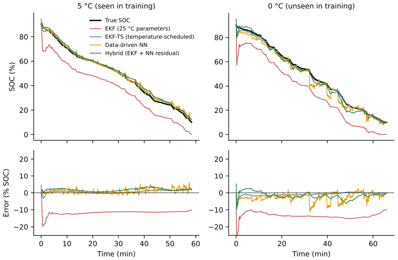
Example runs (mixed cycle, seed 300; conditions fixed before inspection) at 5 °C (seen) and 0 °C (unseen). Top: SOC estimates against truth. Bottom: estimation error. The 25 °C EKF carries a persistent bias of roughly −11 to −15 percentage points; the data-driven network shows jumps after load changes at 0 °C.
Figure 1.
Example runs (mixed cycle, seed 300; conditions fixed before inspection) at 5 °C (seen) and 0 °C (unseen). Top: SOC estimates against truth. Bottom: estimation error. The 25 °C EKF carries a persistent bias of roughly −11 to −15 percentage points; the data-driven network shows jumps after load changes at 0 °C.
3.2. Effect of Temperature
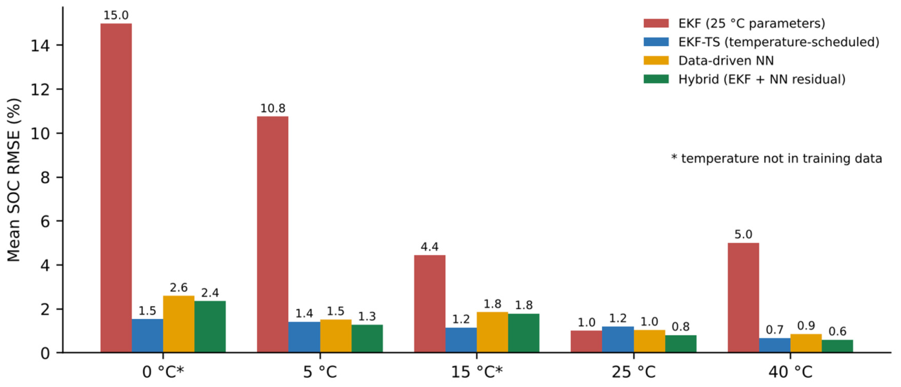
The 25 °C EKF is competitive only at 25 °C, where its parameters were identified, and degrades steeply with distance from it (14.99% at 0 °C). The hybrid was the most accurate method at 5, 25 and 40 °C, but at 0 and 15 °C its error rose to 2.35% and 1.79% while EKF-TS stayed at 1.54% and 1.15%. At 25 °C the hybrid (0.81%) also improved on the 25 °C EKF (1.01%) it is built on, showing that the residual corrects structural error (the unmodelled slow RC branch and hysteresis) in addition to temperature effects.
Table 2.
Mean SOC RMSE (%) by ambient temperature (60 runs per temperature and method).
| Temperature | Coulomb counting | EKF (25 °C) | EKF-TS | Data-driven NN | Hybrid |
| 0 °C (unseen) | 8.54 | 14.99 | 1.54 | 2.59 | 2.35 |
| 5 °C | 10.32 | 10.75 | 1.42 | 1.52 | 1.28 |
| 15 °C (unseen) | 8.28 | 4.45 | 1.15 | 1.85 | 1.79 |
| 25 °C | 8.90 | 1.01 | 1.20 | 1.04 | 0.81 |
| 40 °C | 9.20 | 5.01 | 0.67 | 0.86 | 0.60 |
Figure 2.
Mean SOC RMSE by ambient temperature for the four filters and estimators that use voltage (Coulomb counting omitted). Temperatures marked with an asterisk were absent from training.
Figure 2.
Mean SOC RMSE by ambient temperature for the four filters and estimators that use voltage (Coulomb counting omitted). Temperatures marked with an asterisk were absent from training.
3.3. Robustness to Training Randomness and a Hybrid on Scheduled Physics
Because a single trained network can be unrepresentative, each learned model was retrained with ten random seeds and evaluated on the same 300 runs (Table 3, Figure 3).
The ranking at seen temperatures is stable: hybrid variants (0.88–0.90%) beat both EKF-TS (1.10%) and the data-driven network (1.11%), with small seed-to-seed spread. At unseen temperatures all learned models varied considerably across seeds (standard deviations of 0.22–0.37 points), and none reached EKF-TS (1.34%). Placing the residual on top of the temperature-scheduled physics narrowed the gap (1.60%) and gave the best overall mean (1.17%), statistically indistinguishable from EKF-TS (1.20%) given the seed spread. Its residual was smaller to begin with (17.9 mV versus 80.6 mV), which is consistent with the physics model already absorbing most of the temperature effect.
3.4. Ablation of Residual-Model Inputs and Size
Removing temperature destroyed the benefit (9.00%, close to the uncorrected 25 °C EKF), so the residual is not a generic correction; it is mostly a learned temperature compensation. Removing V1 left seen-temperature accuracy nearly unchanged but more than doubled unseen error (4.39%). Removing I_f, the slow-current feature, did not hurt and gave lower unseen error (1.35%); however, this is a single-seed result and Table 3 shows seed spread of a similar magnitude, so we regard it as a hint that extra history features can encourage over-fitting to the training temperatures rather than as an established effect. Network size had no clear effect over the range tested (mean RMSE 1.21%, 1.15%, 1.32% and 1.28% for networks with 57, 129, 769 and 2,689 parameters, single seed), again within seed noise.
Table 4.
Hybrid RMSE (%) when one input of the residual network is removed (networks retrained, seed 0, 150 test runs from seeds 300–309).
Table 4.
Hybrid RMSE (%) when one input of the residual network is removed (networks retrained, seed 0, 150 test runs from seeds 300–309).
| Residual inputs | Seen T | Unseen T | All |
|---|---|---|---|
| Full (SOC, I, I_f, T, V1) | 0.86 | 2.02 | 1.32 |
| Without slow current I_f | 0.84 | 1.35 | 1.04 |
| Without temperature T | 8.14 | 10.28 | 9.00 |
| Without RC voltage V1 | 0.96 | 4.39 | 2.34 |
| Without SOC | 0.97 | 2.38 | 1.53 |
3.5. Sensitivity to Initial Error and Sensor Quality
Voltage-based estimators forgot the initial SOC error almost immediately: for initial offsets of up to 30% the mean RMSE of EKF, EKF-TS, hybrid and the data-driven network did not change at the reported precision, whereas Coulomb counting rose from 2.5% (no offset) to 19.8% (30% offset). Note that positive offsets are capped by the 100% SOC limit, so the effective positive offset never exceeded 10%.
Table 5.
Mean RMSE (%) under degraded sensors (mixed cycle, five temperatures, five seeds; models and filter settings not retuned).
Table 5.
Mean RMSE (%) under degraded sensors (mixed cycle, five temperatures, five seeds; models and filter settings not retuned).
| Scenario | Coulomb counting | EKF (25 °C) | EKF-TS | Data-driven NN | Hybrid |
|---|---|---|---|---|---|
| Baseline (2 mV, 20 mA bias) | 9.73 | 6.97 | 1.38 | 1.65 | 1.41 |
| Voltage noise 10 mV | 9.73 | 6.97 | 1.39 | 1.70 | 1.42 |
| Current bias 150 mA | 10.50 | 7.10 | 1.56 | 2.31 | 1.91 |
| Both (10 mV; 30 mA noise; 150 mA bias) | 10.50 | 7.10 | 1.56 | 2.35 | 1.91 |
The filters were insensitive to a five-fold increase in voltage noise, which is expected because their tuned measurement-noise settings already assume much larger voltage uncertainty than the simulated noise. A larger current bias degraded the learned estimators more than EKF-TS (hybrid 1.41% to 1.91%; data-driven 1.65% to 2.31%; EKF-TS 1.38% to 1.56%), because the networks use measured current as an input and were trained on low-bias data.
3.6. Computational Cost
On a single CPU thread with pure-Python filters, the EKF took about 2.0 µs per sample and the hybrid about 18.4 µs per sample (finite-difference residual derivatives require three network evaluations per step); the data-driven network, evaluated in batch, took about 1.1 µs per sample. These figures are indicative of relative cost only and do not represent embedded battery-management hardware.
4. Discussion
Three findings stand out. First, a neural-network residual can substantially repair a mismatched physical model: it reduced the error of the 25 °C EKF by roughly 80%. Second, its value is conditional on the baseline. Against a physics model whose parameters were scheduled on temperature, the hybrid helped within the training envelope (0.90% versus 1.10%) but not outside it (1.94% versus 1.34%). The physics-structured extrapolation of EKF-TS used only three fitted parameters per temperature and extended sensibly to 0 °C, whereas the neural network, which has no such structure, did not. Third, the hybrid beat a purely data-driven network trained on the same data at seen temperatures and gave comparable results at unseen temperatures, with lower seed-to-seed variability, which supports the case for embedding learned components in a filter rather than using them alone.
Practical implications follow. When the operating envelope is known and well covered, a residual-corrected EKF is attractive. When it is not, a physically scheduled model is the safer core, and learned corrections should be limited to its smaller remaining error, as the Hybrid-TS result suggests. A deployed hybrid should also detect when temperature leaves its training range and fall back to the physics-only path. The ablation indicates that the residual’s input set matters, with temperature essential, and that adding more history features is not automatically beneficial.
5. Limitations
This is a simulation study, and its conclusions are conditional on the simulator. The ground-truth model is of the same equivalent-circuit family as the estimators, so it does not test structural mismatch with real electrochemistry (diffusion, lithium plating, SOC-dependent hysteresis shape, and so on). Ageing was not simulated, so capacity fade and resistance growth are absent. The drive-cycle-like profiles are synthetic and the thermal model is a single-node approximation. Only one chemistry and one cell size were considered, and only two temperatures were held out. The OCV table is a plausible NMC-like curve, not a measured one. The estimators were given the correct OCV curve at 25 °C. The Hybrid-TS variant was added after inspecting test results, and the one-time extension of the noise-setting grid followed an optimum on its boundary. The 300 test runs share trained models, so the Wilcoxon p-values should not be read as evidence about training randomness, for which Table 3 is the better guide. The computational comparison is indicative only. Experimental validation on cycling data over a range of temperatures is the necessary next step.
6. Conclusions
In a controlled simulation, adding a neural-network voltage residual to an extended Kalman filter reduced SOC error from 7.24% to 1.37% RMSE, outperformed a purely data-driven network overall, and was the most accurate method at the temperatures present in training. A simpler physics-only filter with temperature-scheduled parameters nevertheless generalized better to unseen temperatures, and a hybrid built on that scheduled model matched it overall. The practical lesson is that the hybrid’s advantage is real but bounded by its training coverage, and that a strong physics baseline should always accompany claims of hybrid improvement. These findings require confirmation with experimental data.
Author Contributions
Misker Shumeye conceived and supervised the study. All authors reviewed and approved the final manuscript.
Funding
This research received no external funding.
Data and Code Availability
All data are generated by the simulation code (core.py, run_all.py, extra.py, analyze.py), which reproduces every table and figure. The simulation code is available from the corresponding author on reasonable request.
Competing Interests
The authors declare no competing interests.
References
- Hannan, M.A.; Lipu, M.S.H.; Hussain, A.; Mohamed, A. A review of lithium-ion battery state of charge estimation and management system in electric vehicle applications: Challenges and recommendations. Renewable and Sustainable Energy Reviews 2017, 78, 834–854. [CrossRef]
- Xiong, R.; Cao, J.; Yu, Q.; He, H.; Sun, F. Critical review on the battery state of charge estimation methods for electric vehicles. IEEE Access 2018, 6, 1832–1843. [CrossRef]
- Waag, W.; Fleischer, C.; Sauer, D.U. Critical review of the methods for monitoring of lithium-ion batteries in electric and hybrid vehicles. Journal of Power Sources 2014, 258, 321–339. [CrossRef]
- Plett, G.L. Extended Kalman filtering for battery management systems of LiPB-based HEV battery packs: Part 1. Background. Journal of Power Sources 2004, 134, 252–261.
- Chemali, E.; Kollmeyer, P.J.; Preindl, M.; Emadi, A. State-of-charge estimation of Li-ion batteries using deep neural networks: A machine learning approach. Journal of Power Sources 2018, 400, 242–255. [CrossRef]
- Ng, M.-F.; Zhao, J.; Yan, Q.; Conduit, G.J.; Seh, Z.W. Predicting the state of charge and health of batteries using data-driven machine learning. Nature Machine Intelligence 2020, 2, 161–170. [CrossRef]
- Raissi, M.; Perdikaris, P.; Karniadakis, G.E. Physics-informed neural networks: A deep learning framework for solving forward and inverse problems involving nonlinear partial differential equations. Journal of Computational Physics 2019, 378, 686–707. [CrossRef]
- Tu, H.; Moura, S.; Wang, Y.; Fang, H. Integrating physics-based modeling with machine learning for lithium-ion batteries. Applied Energy 2023, 329, 120289. [CrossRef]
- Singh, S.; Ebongue, Y.E.; Rezaei, S.; Birke, K.P. Hybrid modeling of lithium-ion battery: Physics-informed neural network for battery state estimation. Batteries 2023, 9, 301. [CrossRef]
- Tao, J.; Wang, S.; Cao, W.; Fernandez, C.; Blaabjerg, F. A comprehensive review of multiple physical and data-driven model fusion methods for accurate lithium-ion battery inner state factor estimation. Batteries 2024, 10, 442. [CrossRef]
- Takyi-Aninakwa, P.; Wang, S.; Zhang, H.; Li, H.; Xu, W.; Fernandez, C. An optimized relevant long short-term memory-squared gain extended Kalman filter for the state of charge estimation of lithium-ion batteries. Energy 2022, 260, 125093. [CrossRef]
- Wang, C.; Li, R.; Cao, Y.; Li, M. A hybrid model for state of charge estimation of lithium-ion batteries utilizing improved adaptive extended Kalman filter and long short-term memory neural network. Journal of Power Sources 2024, 620, 235272. [CrossRef]
- Liu, D.; Wang, S.; Li, X.; Fan, Y.; Fernandez, C.; Blaabjerg, F. A novel extended Kalman filter-guided long short-term memory algorithm for power lithium-ion battery state of charge estimation at multiple temperatures. Energy 2025, 335, 137973. [CrossRef]
Figure 3.
Per-seed mean RMSE for ten training seeds at seen and unseen temperatures; horizontal bars mark seed means and the dashed line marks EKF-TS.
Figure 3.
Per-seed mean RMSE for ten training seeds at seen and unseen temperatures; horizontal bars mark seed means and the dashed line marks EKF-TS.
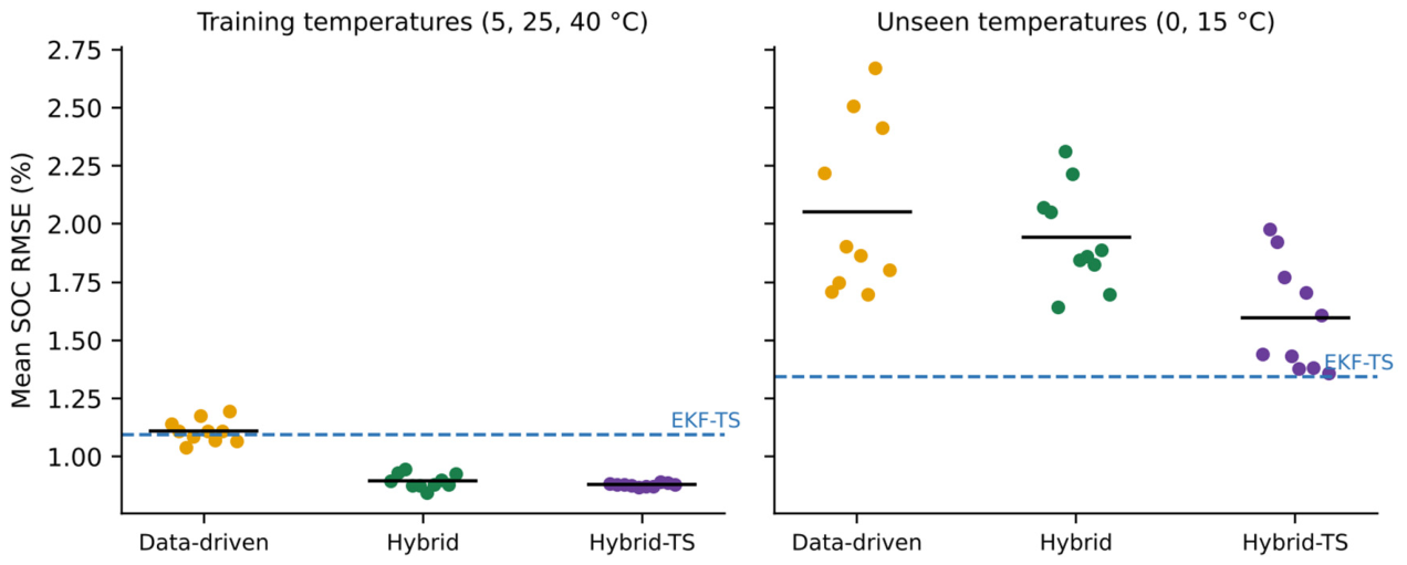
Table 3.
Mean RMSE (%) across ten training seeds (mean ± standard deviation of the per-seed mean RMSE).
Table 3.
Mean RMSE (%) across ten training seeds (mean ± standard deviation of the per-seed mean RMSE).
| Method | Seen temperatures | Unseen temperatures | All |
| Data-driven NN | 1.11 ± 0.05 | 2.05 ± 0.37 | 1.49 ± 0.17 |
| Hybrid | 0.90 ± 0.03 | 1.94 ± 0.22 | 1.31 ± 0.08 |
| Hybrid-TS (post-hoc) | 0.88 ± 0.01 | 1.60 ± 0.23 | 1.17 ± 0.09 |
| EKF-TS (no training randomness) | 1.10 | 1.34 | 1.20 |
Disclaimer/Publisher’s Note: The statements, opinions and data contained in all publications are solely those of the individual author(s) and contributor(s) and not of MDPI and/or the editor(s). MDPI and/or the editor(s) disclaim responsibility for any injury to people or property resulting from any ideas, methods, instructions or products referred to in the content. |
© 2026 by the authors. Licensee MDPI, Basel, Switzerland. This article is an open access article distributed under the terms and conditions of the Creative Commons Attribution (CC BY) license (http://creativecommons.org/licenses/by/4.0/).
Copyright: This open access article is published under a Creative Commons CC BY 4.0 license, which permit the free download, distribution, and reuse, provided that the author and preprint are cited in any reuse.