
Submitted:
17 November 2026
Posted:
18 November 2026
You are already at the latest version
Abstract
This paper presents a model of the operation and maintenance process of means of transport in an urban public transport system and the results of its simulation. The process is described by a semi-Markov model identified on the basis of source documents and operational tests carried out in a real urban transport system. The model is defined by the transition probability matrix for the operation and maintenance states (among others, those of carrying out transport tasks, servicing and repairs), the distributions of the sojourn times in the states, and the unit revenues and expenditures associated with the sojourn in them. An algorithm and a program have been developed for simulating realisations of the stochastic process, in which the sojourn times in the states are generated from a gamma distribution with parameters determined on the basis of the research results. In the first example, simulation runs were compared for two groups of buses differing in their period of operation. The share of driving time in the total simulation time proved to be significantly greater for the new buses, which is consistent with the observational data. In the second example, experiments were carried out in which the transition matrices and the parameters of the sojourn time distributions were swapped between the two groups, and it was investigated how the mean value of the sojourn time in the state of active use affects the total sojourn times in the individual states and the profit from the operation of the buses. The results confirm the influence of the period of operation of the buses and of the mean sojourn time in the state of active use on the efficiency of the operation and maintenance process. The proposed model can support the assessment of the operating efficiency of the transport system and the making of operation and maintenance decisions and, owing to the generality of its description, it can also be used in systems other than urban bus transport.
Keywords:
system
; operation and maintenance process
; process model
; semi-Markov process
; transport system
; urban public transport
; stochastic process
1. Introduction
The use of operations research to analyse the cycle of events occurring in the operation and maintenance process of machines can provide a proper basis for making rational decisions for controlling the system that carries out this process [1]. The optimisation of activities concerns keeping machines in a state of task serviceability at the required level of technical availability.
For complex technical systems, methods based on computer simulation of the processes carried out in these systems are among the more useful ones used to obtain the information necessary for making rational decisions for controlling these systems and for optimising activities related to keeping technical objects in a state of task serviceability at the required level of technical availability [2,3].
The complex technical system under consideration is the operation and maintenance system of means of transport in urban public transport. The process analysed, which is carried out in this system, is the operation and maintenance process of urban public transport buses.
The usefulness of the research results obtained by simulating operation and maintenance processes depends to a large extent on the adequacy of the process model used and on the accuracy with which the values of the parameters needed to carry out the simulation runs of the process are estimated. The analysis is based on a model of the process carried out in the transport system, described in terms of states and possible transitions between these states. The states of the process are characterised by sojourn time distributions and by the costs incurred, which depend on the type of state [4,5]. The basic data needed to simulate the operation and maintenance process were obtained from operational tests conducted under the natural operating conditions of urban public transport buses.
The operation and maintenance process of means of transport, described in terms of operation and maintenance states and the transitions between them, is most often modelled using Markov and semi-Markov processes. The contribution of applications of semi-Markov processes to reliability and to the operation and maintenance of technical objects was systematically described in [6]. For many years, simulation models of the operation and maintenance process of the class of technical objects under consideration, including urban public transport buses, have been developed and the influence of decision and control variables on the efficiency of this process has been studied, as presented in [4] and [7,8,9,10,11,12]. Subsequent papers presented, inter alia, a numerical simulation of the process of changes in the states of a technical object [13], a method of controlling availability in a transport system using a simulation model of the operation and maintenance process [14], a method for the preliminary estimation of the unit costs of the sojourn of urban means of transport in operation and maintenance states [5], and the modelling of the operation and maintenance process of city buses by means of homogeneous Markov processes [15]. Semi-Markov models of renewal systems of technical objects, including city buses, which take into account repairs and preventive replacements, with criteria of availability and profit per unit time, were presented in [16,17].
Increasing attention is being paid to the identification of such models on the basis of data from real transport systems. In [18], logistic regression was proposed for determining the transition probability matrix for the operation and maintenance states, taking into account the dependence of the transitions on the sojourn time of the object in the given state. In [19], a simulation model of the operation and maintenance process of vehicles in a transport system was developed in which the sojourn time distributions in the states were selected on the basis of empirical data, and the simulation results were compared with those of a semi-Markov model. Simulation methods in the analysis of the reliability and availability of technical systems were presented in [20]. Studies of urban public transport buses operated under real conditions indicate significant differences in technical availability and reliability between groups of vehicles, inter alia between bus makes in the post-warranty period [21] and between electric and internal combustion engine buses [22]. The general theory of semi-Markov processes is also being developed: recent monographs have presented, among others, coupling and ergodic theorems for semi-Markov-type processes [23], as well as discrete-time semi-Markov random evolutions and their applications [24]. Methods for determining the characteristics of semi-Markov processes using approximating semi-Markov chains [25] and kernel estimators of the Markov renewal function and of the transition functions of semi-Markov systems [26] have also been developed. Semi-Markov models are used to describe the reliability and the operation and maintenance process of technical objects, including in a non-homogeneous formulation [27], as well as of vehicles operated in transport systems [28].
In the works cited, the influence of the structure of transitions between states (the transition probability matrix) is relatively rarely separated from the influence of the sojourn time distributions in the states on the efficiency indicators of the operation and maintenance process of vehicle groups differing in their period of operation. The aim of this paper is to carry out a simulation analysis of the operation and maintenance process of urban public transport buses using a multi-state semi-Markov model identified on the basis of source documents and operational tests in a real urban transport system. The contribution of the paper comprises: an algorithm and a program for simulating realisations of the process with gamma distributions of the sojourn times in the states, a comparison of simulation results for the “New” and “Old” buses, simulation experiments in which the transition matrices and the parameters of the sojourn time distributions are swapped between the two groups, and an analysis of the influence of the mean value of the sojourn time in state S1 on the profit from operation.
2. Research Object
The research object is a complex operation and maintenance system of means of transport. Controlling the implementation of operation and maintenance processes in this system makes it possible to achieve the set goal. Therefore, this system is an action system with goal-oriented behaviour. The analysed research object is a real urban transport system, i.e. the Bus Transport Company (ZKA), and the bus operation and maintenance process carried out in this system. Buses of various types are operated in the Bus Transport Company.
The primary goal of the identified system is to carry out passenger transport that is efficient (in terms of the economic criterion) and safe, within the quantitative and territorial scope set by the superior system, using the technical objects operated in the system.
The following tasks are carried out in the Bus Transport Company:
- planning activities and managing their implementation,
- controlling the use of vehicles (and of other technical objects supporting these activities),
- keeping vehicles in running order,
- providing logistic support for the activities of the system,
- storing vehicles.
It is a system with a hierarchical structure of the <C-OT> (human – technical object) type. An integral part of the ZKA is the vehicle service station (understood as an anthropotechnical subsystem – people + technical objects), whose operation is managed by the service station manager. Preventive activities concerning vehicles (daily servicing, diagnosing, adjustments) and repairs (routine, failure-related, other) are carried out at the vehicle service station.
Preventive activities and repairs of vehicles are performed at the repair stands of the service station or by technical emergency units (PT units) outside the ZKA premises.
The identification of the functioning of the ZKA and the analysis of the values of the efficiency indicators calculated for 160 buses over a period of 200 days show that the vehicle operation and maintenance process is carried out in the system according to a low-efficiency strategy from the point of view of the possibility of exploiting the use potential.
Four subsystems were distinguished in the studied operation and maintenance system (SE):
- use,
- control,
- serviceability assurance,
- diagnostic.
The goal of the operation and maintenance system is achieved directly by the use subsystem, which comprises the technical objects together with their operators.
The operation and maintenance control subsystem performs the function of directing and supervising the functioning of the operation and maintenance system. Servicing, and in particular renewal, is carried out by the serviceability assurance subsystem.
The role of the diagnostic subsystem, which cooperates with the serviceability assurance subsystem, consists in examining diagnostic signals and symptoms in order to determine the past, current or future states of the operated technical objects, as well as in assessing the performance of their operators and identifying the states of the environment.
Since the operation and maintenance system is a complex and multi-task system (one that performs many tasks), it can, depending on the state of its subsystems, perform all or some selected tasks.
The environment of the system, whose influence facilitates or prevents the performance of tasks by the system, was also taken into account. For this reason, the environment of the studied operation and maintenance system was treated as one of the subsystems cooperating with the studied system and was included in the model describing the significant (from the point of view of efficiency) states of the operation and maintenance process of technical objects.
The most important activities and processes that significantly affect the correctness and efficiency of the bus operation and maintenance process are the processes of use, serviceability assurance and diagnosing.
Preventive activities, comprising primarily daily servicing, diagnostic inspections of the condition of the vehicles and adjustments, are performed at service stations by specialised staff. Depending on their labour intensity, vehicle repairs are carried out either at vehicle service stations or by technical emergency units belonging to the Bus Transport Company. If the technical emergency service cannot repair the damaged vehicle within the city, the vehicle drives or is towed to the service station.
The basic sources of operational information are archived in-house documents describing the states in which the buses reside.
3. Model Description
The model of the operation and maintenance process was built on the basis of an analysis of the space of operation and maintenance states and of the operation and maintenance events concerning urban public transport buses operated in a real urban transport system.
The model of the operation and maintenance process was described in terms of states and possible transitions between these states. The states of the process are characterised by the distributions of sojourn times and by the profits (losses) associated with the sojourn of technical objects in the distinguished states [4].
Owing to the limited length of the paper, only the basic assumptions of the developed model are presented.
Let S1, S2, ..., Sg (g ∈ N) denote the distinguished significant operation and maintenance states in which technical objects can be found.
Each of the operated technical objects can, at a given instant of time t, t ∈ R+, be in only one of the distinguished states. The sojourn of objects in the individual states generates revenues and/or expenditures associated with the functioning of the system.
A realisation of the process is a sequence of successive distinguished states. The order in which the states follow one another, the sojourn times in the individual states and the frequencies of their occurrence depend primarily on the individual characteristics of the particular technical objects, on the characteristics of the processes to which these objects are subject, and on the characteristics and structure of the subsystems cooperating in the implementation of the operation and maintenance process.
On the basis of an analysis of the urban bus transport system and the operation and maintenance process carried out in it, as well as the identification of the space of states and events concerning the means of transport in use, the following operation and maintenance states of the bus were distinguished [4]:
S1 – state of active use of the technical object (carrying out the transport task),
S2 – state of the technical object waiting for a technical emergency unit,
S3 – state of renewal of the technical object carried out in the environment of the operation and maintenance system,
S4 – state of the technical object waiting for renewal carried out in the operation and maintenance system,
S5 – state of renewal of the technical object carried out in the operation and maintenance system,
S6 – state of the technical object waiting for diagnosing,
S7 – state of diagnosing the technical object,
S8 – state of daily servicing of the technical object,
S9 – state of the technical object waiting to undertake the transport task,
S10 – state of the technical object waiting due to the unserviceability of the environment,
S11 – state of organisational standstill of the technical object.
As a result of the identification of the system and of the multi-state operation and maintenance process of technical objects carried out in it, the significant states of this process were distinguished on the basis of the criterion of state significance. The states of this process analysed in the simulation model of the operation and maintenance process correspond to the operation and maintenance states of the technical objects. Each of the operated technical objects can, at a given instant of time, be in only one of the model states described below:
S1 – State of Intensive Use of the Technical Object
The state of intensive use of the technical object is the state in which the <OT>, together with its operator, carries out the transport task assigned to them.
In the studied urban transport system, defining the daily transport task for a given technical object and operator consists in assigning a route number and run numbers. The territorial scope of the transport task is determined by the route number, whereas its temporal scope is determined by the run numbers in accordance with the applicable timetable.
S2 – State of the Technical Object Waiting for a Technical Emergency Unit
The state of the technical object waiting for a technical emergency unit is the state in which a task-unserviceable technical object located in the environment of the SE (in the territorial sense) waits for the arrival of a PT unit or, together with its operator, moves to the place where the PT unit is stationed.
S3 – State of Renewal of the Technical Object Carried out in the Environment of the Operation and Maintenance System
The state of renewal of the technical object carried out in the environment of the operation and maintenance system is the state in which a task-unserviceable technical object located in the environment of the operation and maintenance system is subject to actions aimed at restoring its state of task serviceability. In the studied urban transport system, the actions aimed at restoring the state of task serviceability of a technical object located in the environment of the operation and maintenance system are understood to include, in particular:
- renewal carried out by PT units,
- towing of the vehicle by PT units to a diagnostic station or service station (belonging to the SE),
- emergency return of the vehicle to a diagnostic station or service station.
S4 – State of the Technical Object Waiting for Renewal Carried out in the Operation and Maintenance System
The state of the technical object waiting for renewal carried out in the operation and maintenance system is the state in which a task-unserviceable technical object located in the operation and maintenance system (in the territorial sense), after being submitted for renewal, waits for the renewal process to begin.
S5 – State of Renewal of the Technical Object Carried out in the Operation and Maintenance System
The state of renewal of the technical object carried out in the operation and maintenance system is the state in which a technical object located in the operation and maintenance system undergoes renewal.
S6 – State of the Technical Object Waiting for Diagnosing
The state of the technical object waiting for diagnosing is the state in which a technical object located in the operation and maintenance system, after being submitted for diagnosing, waits for the diagnosing process to begin.
S7 – State of Diagnosing the Technical Object
The state of diagnosing the technical object is the state in which a technical object located in the operation and maintenance system undergoes the diagnosis process. Diagnosing a technical object located in the operation and maintenance system is understood to include, in particular:
- so-called pre-repair diagnosing (when the object is in the state of task unserviceability),
- so-called post-repair diagnosing (as a check of the correctness of the renewal process),
- so-called anticipatory diagnosing (aimed at preventing the occurrence of failures while the technical object is carrying out the transport task, and resulting from the operation and maintenance strategy being implemented).
S8 – State of Daily Servicing of the Technical Object
The state of daily servicing of the technical object is the state in which activities related to the so-called daily servicing of the technical object, resulting from the operation and maintenance strategy applied, are carried out.
S9 – State of the Technical Object Waiting to Undertake the Transport Task
This is the state in which, immediately after its state of task serviceability has been restored or after a change in the state of the environment of the operation and maintenance system, the means of transport waits to undertake the transport task.
S10 – State of the Technical Object Waiting Due to the Unserviceability of the Environment
The state of the technical object waiting due to the unserviceability of the environment is the state in which a task-serviceable technical object does not carry out the planned transport task as a result of an event occurring in the environment of the SE that prevents this task from being carried out (unserviceability of the environment of the operation and maintenance system, e.g. weather conditions).
S11 – State of Organisational Standstill of the Technical Object
The state of organisational standstill of the technical object is the state in which the technical object is not in any of the previously distinguished states. In the studied system, the sojourn time in the state of organisational standstill of the technical object is understood to include, in particular:
- the parking time of a serviceable vehicle resulting from the specific nature of the transport tasks (the adopted timetable),
- the waiting time of an unserviceable vehicle (on the depot premises) for renewal due to a lack of spare parts.
Each of the states is assigned a distribution of the sojourn time in that state, characterised by the mean value and the standard deviation.
The gamma, Weibull or log-normal distribution, with appropriately selected parameters determined on the basis of the results of operational tests, was adopted as the basic type of distribution of the sojourn times in the distinguished states [19].
The sojourn time of an object in each of the model states is therefore generated according to a gamma distribution with a specific mean value and standard deviation characteristic of the given state [29].
In addition to the characteristics of the states, the possible transitions between the states were determined in the process of identifying the operation and maintenance system, as shown in Figure 1.
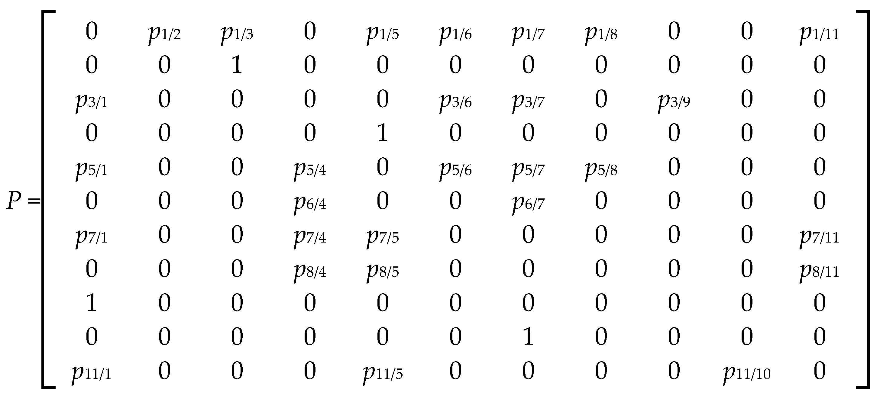
Each arc of the graph connecting two states is associated with the value of the probability of the process transition from state i = 1,2,...,11 to state j = 1,2,...,11 at a random instant of time t. The matrix of the probabilities of changes in the process states has the form:
The course of the operation and maintenance process in the system under study is specific to each object because – as indicated above – it depends both on the features of the objects themselves and on the structure of the cooperating subsystems. Therefore, when assessing the efficiency of the operation and maintenance process of technical objects, both the economic and the technical aspects of the functioning of the systems and of the processes carried out in these systems should be taken into account.
4. Assumptions of the Mathematical Model
A stochastic process is developed that will be the mathematical model of the operation and maintenance process of the object. Let {X(t), t ≥ 0} be a stochastic process with the set of states {S1, S2, ..., Sk}, and let 0 = τ0 < τ1 < τ2<…<τn<… be random variables denoting the instants at which the changes of state of this process occur. It is assumed that, for a known state of the process at instant τn, the duration of the given state and the state reached at instant τn+1 are stochastically independent of the states of the process at instants τ0,τ1,…,τn−1 and of the durations of the previous states. The above statement can be written as follows:
where:
j,i, in-1, in-2, ... i1, i0 ∈ {1, 2, ..., k} n ∈ N.
This equality means that the process X(t) is a semi-Markov process [6,30]. A semi-Markov process is fully determined when the matrix of functions Q(t) of the following form is given:
called the kernel of the process, and when the initial distribution of the following form is given:
It follows from the theory of semi-Markov processes that the sequence of random variables X(τn),n ∈ N is a homogeneous Markov chain with the transition probability matrix,
This chain is called the embedded Markov chain of the process X(t).
The random variables Ti, 1 ≤ i ≤ k, denoting the durations of the process states, are important characteristics of a semi-Markov process. The cumulative distribution functions of the variables Ti have the form:
It is assumed that the random variables Ti have probability densities fi(t).
The operation and maintenance process of technical objects carried out in the transport system, analysed in this study, is observed over a sufficiently long time interval < 0, t >. In view of the above, a limit theorem of the following form is used in this paper [30]:
if the semi-Markov process X(t) with a finite set of states S = {S1, S2, ..., Sk} is irreducible and the random variables Ti, 1 ≤ i ≤ k have finite and positive mean values ETi, then there exists a limiting distribution of the process X(t) of the form:
for every j ∈ {1, 2, ..., k}, and it is expressed by the formula:
The probabilities pi* (1 ≤i≤ k) are the ergodic probabilities of the embedded Markov chain, and they are determined as the solution of the system of linear equations of the form:
The system of linear equations (9) is a dependent system. In order to determine the limiting probabilities pi*, one of the equations of system (9) should be replaced by the normalisation condition (10).
Let zi, i = 1, 2, ..., k denote the revenue (expenditure) resulting from the operation of one object per unit time when the object is in state Si.
Further, let Hi(t) denote the total sojourn time of the process X(t) (of the object) in state Si in the time interval < 0, t >. The expression:
denotes the profit from the operation of the object in the time interval < 0, t >, whereas the expression:
denotes the mean income from the operation of the object in the interval < 0, t >. The value Eh(t)/t denotes the mean income from the operation of the object per unit time.
For sufficiently large t, instead of the ratio Eh(t)/t, it is more convenient to study its limit of the form:
The value h (if it exists) denotes the mean income per unit time resulting from the operation of the object (when its operation and maintenance process is analysed over a sufficiently long time interval).
It is known from [31] that, under certain general assumptions, the following limit exists:
Hence, taking into account Equations (11)–(14), it follows that:
Taking into account assertion (8) of the limit theorem for semi-Markov processes, we obtain:
The mathematical model of the operation and maintenance process of technical objects is the stochastic process {X(t), t ≥ 0} with a finite set of states S. If X(t) = Si (i = 1, 2, ..., g), then the technical object under consideration is in state Si at instant t. In this paper, it is assumed that the process X(t) is a semi-Markov process.
In using semi-Markov processes for the mathematical modelling of the operation and maintenance process, the following main assumptions were adopted:
- the semi-Markov process represents the modelled real operation and maintenance process sufficiently well from the point of view of the research objective,
- the modelled operation and maintenance process has a finite number of states,
- the random variables denoting the durations of the distinguished process states have finite and positive mean values and variances,
- the distinguished states of the operation and maintenance process are positive recurrent states,
- the random process X(t), which is the mathematical model of the operation and maintenance process, is homogeneous.
The analysed process X(t) (a homogeneous semi-Markov process) is fully determined when the following are given [6,30]: the initial distribution of the process P0, the matrix P of transition probabilities between the process states, i.e. the transition probability matrix of the embedded Markov chain, and the cumulative distribution functions of the random variables Tij, where Tij is the random variable denoting the sojourn time of the technical object in state Si, given that the next state is state Sj.
5. Description of the Simulation Method
The simulation of the process of changes in the operation and maintenance states of the technical object consists in generating realisations of the described stochastic process, which is the model of the operation and maintenance process [2,13,20].
The process simulation program was developed on the basis of the following preliminary assumptions. A single technical object (bus) is characterised by the properties listed below:
| – state | – natural number (state index) assigned to each object under study; |
| – time | – real variable in which the generated time in each of the states except state S1 is stored; |
| – driving time | – real variable in which the generated driving time (in state S1) is stored; |
| – ta | – local time of the research object, increasing continuously from the start of the simulation to the end of the simulation run. |
At the start of the simulation, the technical object is in state S1. In this state, a driving time is generated for it in accordance with the determined parameters and type of distribution. Next, a number is generated from the uniform distribution on the interval [0, 1] in order to determine, on this basis and on the basis of the values of the transition probabilities contained in the first row of the transition matrix, the next state [32]. The transition to this state takes place after the generated driving time has elapsed.
This cycle is repeated for each state in which the object finds itself after a change of state. Each row of the transition matrix determines subintervals on the interval [0, 1] in the following way: let the row contain the numbers x1, x2, ..., xk such that, for every k, xk < 1, and = 1.
The subintervals are then determined as follows:
[0,x1), [x1,x1+x2), [x1+x2,x1+x2+x3),....
The number m, drawn from the uniform distribution on the interval [0, 1), belongs to one of the described subintervals. At the same time, this makes it possible to determine the next state of the object.
It should be emphasised that the scheme is simplified and does not take into account all the conditions that occur in the real bus operation and maintenance system.
Among other things, the fact that the buses run for 19.5 h a day and spend 4.5 h in the depot is not reflected. However, the simulation program has been written in such a way that it can take these dependencies into account.
In the simulation process, it is also possible to take into account, as an option, the fact that the generated driving time of a bus is much longer than the times generated in states other than S1. As a result, a bus failure event occurs in the simulation process once every few days. Taking this fact into account, an “End of day” procedure was introduced in the simulation program, which is executed when the object ends the current working day in the state of serviceability. The procedure sets the object to state S8 (i.e. the state of daily servicing of the technical object). On the following day, the object will be in state S1 (at the beginning of the day) with the driving time reduced by the value that was realised on the preceding days. When the generated driving time of the object has elapsed, the object changes its state S1 to the states (S2∨S3∨S5∨S6∨S7∨S8∨S11) with the probability resulting from the generated number m and the first row of the transition matrix.
One of the basic objectives of the simulation program is the statistical analysis of the array (matrix) Tr[ij], where i = 1,2,...,k, j = 1,2,...,n, k – number of states of the modelled system, n – number of objects (vehicles) in the system. Tr[i,j] denotes the total sojourn time of the j-th object in state Si. For all states Si, i = 1, 2, ..., k, the values of the following statistics are determined in turn:
- the mean total sojourn time of a random object in state Si,
- the standard deviation of this time,
- the coefficient of variation as the ratio of the standard deviation to the mean value,
- the mean normalised absolute deviation, calculated for the random sample x1,x2,...xn according to the formula:
– sample mean value,
s – sample standard deviation;
- the skewness of the distribution, determined according to the formula:
The last two statistics form the basis for verifying the hypothesis that the distribution of the total sojourn time in each of the states is a normal distribution [33]. This results from the fact that the random variables Tr[i,j], denoting the total sojourn time of the object in state Si, i = 1, 2, ..., k, are sums of independent random variables with the same distribution. This means that the assumptions of the Lindeberg–Lévy version of the central limit theorem are satisfied for Tr[i,j].
The values of the basic statistics listed above were also determined for the random sequence zr[j], j = 1, 2, ..., n, expressing the unit revenues (expenditures) for the individual objects.
6. Discussion of the Results of the Simulation Model Studies
Two groups of vehicles, conventionally named “New” (max. 2 years of operation) and “Old” (period of operation of up to 8–10 years), were randomly selected for the analysis.
The aim of the example is to verify the simulation results for both bus groups (“New” and “Old”), which differ significantly in their operational parameters. The share of driving time in the total simulation time was adopted as the evaluation indicator.
The input data for the simulation were estimated on the basis of the preliminary operational tests carried out in the research object.
Different types of objects and different periods of use to date were analysed. The analysis of the functioning of the constructed simulation model shows that there is a close relationship between the value of the unit profit function and the technical activities carried out, which result from the adoption of an appropriate operation and maintenance strategy.
The determined parameters characterising the sojourn times in the individual states are presented in Table 1, while the estimated values of the elements of the transition probability matrix P (with the structure defined by Equation (1)) are given below. Since in this example the two bus groups differ only in the mean sojourn time in state S1, a common matrix P was adopted for them. Its elements were estimated by the maximum likelihood method as the ratios of the total number of transitions from state Si to state Sj to the total number of exits from state Si, recorded in the operational tests of the subsets of “Old” and “New” buses (the estimates made separately for the two subsets are presented in the form of the matrices given by Equations (22) and (23)).
The estimated values of the elements of matrix P are presented in matrix :
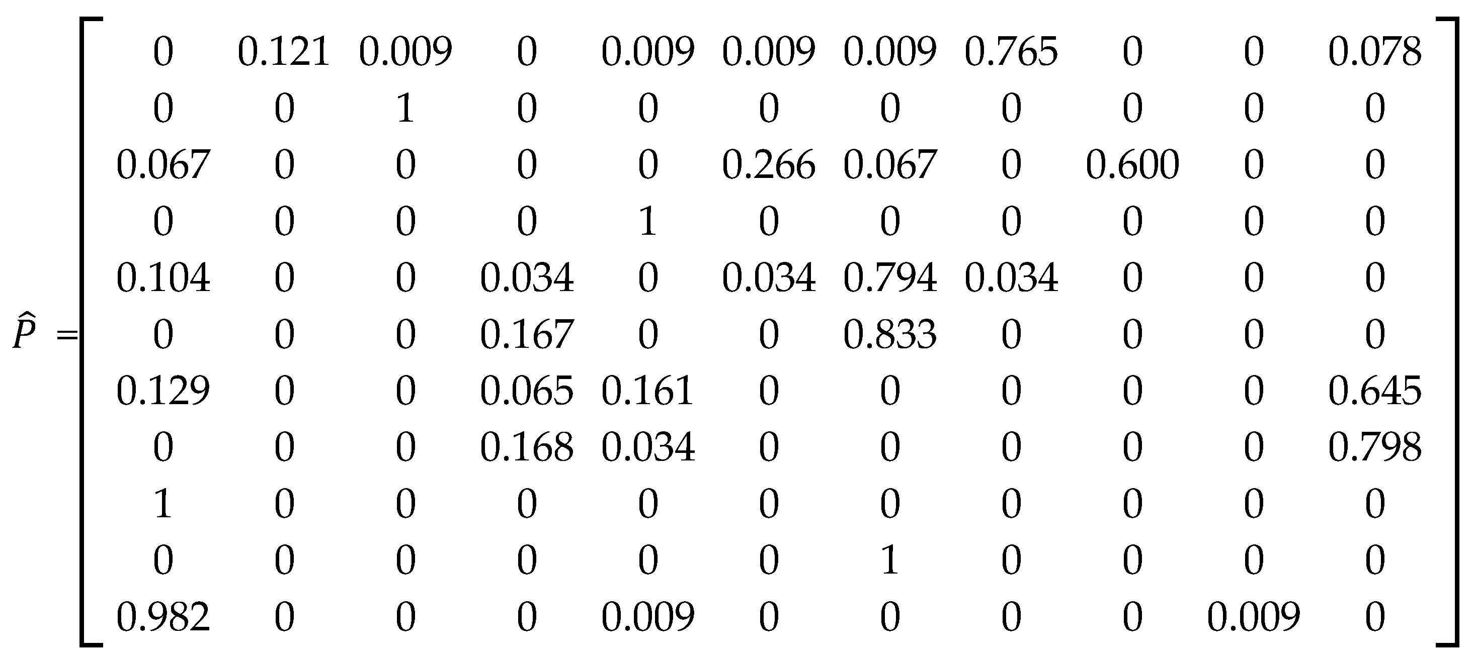
As can be seen in matrix P described by Equation (1), some of its rows contain ones, which means that the transition from the state corresponding to the given row of the matrix to the state corresponding to the given column is a certain event. In Figure 1, these correspond to the transitions represented by the directed arcs connecting the states: S2→S3; S4→S5; S9→S1; S10→S7.
Note that in column S8 of the transition matrix, the only non-zero elements are those corresponding to rows S1 and S5, i.e. the process can move to state S8 only from state S1 or from state S5. This state is reached when the research object has finished work (S1) on a given day and, without having suffered a failure, has returned to the parking yard, or after the completion of the renewal carried out in the operation and maintenance system (S5).
The adoption of a random number generator with a gamma distribution in the model was based on an analysis of the observational data for both of the above-mentioned bus groups (“New” and “Old”). The parameters of the gamma distributions (shape and scale) for the individual states were determined by the method of moments, i.e. from the mean values and standard deviations given in Table 1.
It was further assumed that the simulation run lasts until the variable ta (the local time of the object) exceeds the value Tmax, which denotes the end of the run (Figure 2). The number of objects for which the simulation run was performed was set at 100 units, and the simulation time Tmax at 100 days.
In the simulation runs for the “New” and “Old” bus groups, the distinguishing parameter was the mean time spent in state S1 (driving). The standard deviation of this time, as well as the mean sojourn times in the remaining states and their standard deviations, were assumed to be identical for both groups.
Five simulation runs were carried out for each of the groups. The operation and maintenance process of 100 objects was analysed. The results obtained are presented in Table 2.
In order to verify the hypothesis that significantly different mean values of the indicator (% of driving time) were obtained in the simulation runs for the two bus groups, a test for two means was carried out with the following hypotheses (μ1, μ2 – expected values of the indicator for the “Old” and “New” buses, respectively):
H0: the mean values of the indicator in both groups are equal (μ1 = μ2),
H1: the mean for the “Old” buses is lower (μ1 < μ2).
On the basis of the results of the five simulation runs for each group, the mean values of the indicator were calculated. They are m1 = 92.914 and m2 = 94.384 for the “Old” and “New” buses, respectively, and the difference of the means is m2 − m1 = 1.47. The sample variances (unbiased estimators, with the divisor n − 1 = 4) have the values s12 = 0.0287 and s22 = 0.0234, respectively.
The sample sizes are small (n1 = n2 = 5), and the variances of the indicator in the two groups are unknown and are not assumed to be equal; therefore, Welch’s t-test was applied. Using the statistic:
where n1 and n2 denote the sample sizes. Under the assumption that hypothesis H0 is true, this statistic approximately follows Student’s t distribution with the number of degrees of freedom ν given by the Welch–Satterthwaite formula:
we obtain ν ≈ 7.92 and the value of the statistic t = −14.41.
Assuming the significance level α = 0.01 (i.e. assuming that the probability of rejecting the tested hypothesis H0 when it is true is equal to 0.01) and reading the critical value tα from the table of Student’s t distribution for ν = 8 degrees of freedom (the rounded value of ν ≈ 7.92), taking into account the left-tailed critical region, we obtain tα = −2.90. Since t = −14.41 < tα, the statistic lies in the critical region, i.e. the tested hypothesis of equal means should be rejected in favour of hypothesis H1.
Note, moreover, that even for a very low significance level α = 0.001 (critical value tα = −4.50 for ν = 8), the hypothesis would also have to be firmly rejected, since the observed significance level of the test (the p-value) is approx. 3·10−7. The same conclusion is given by the classical Student’s t-test assuming equal variances (with the pooled variance sp2 = 0.0260): for equal sample sizes (n1 = n2), its statistic takes the same value t = −14.41, with 8 degrees of freedom. We can therefore conclude that the obtained difference in means (1.47 percentage points) is statistically significant.
A further aim of the simulation experiment was:
a) to verify the hypothesis concerning the influence of the length of the period of operation of the buses on the efficiency of the operation and maintenance process carried out in the urban public transport system;
b) to verify the hypothesis concerning the influence of the mean value of the sojourn time in state S1 (state of active use of the technical object) on the efficiency of the operation and maintenance process.
In order to achieve the aims of the experiment, two transition probability matrices and two sets of values of the parameters characterising the sojourn times of the vehicles in the individual states of the operation and maintenance process were estimated. The above-mentioned quantities were estimated on the basis of the source documents used in a real operation and maintenance system of urban transport, i.e. at the ZKA in Bydgoszcz, and of the operational tests carried out. An alternative method of estimating the transition probability matrix, which takes into account the dependence of the transitions on the sojourn time of the object in the state, is presented in [18].
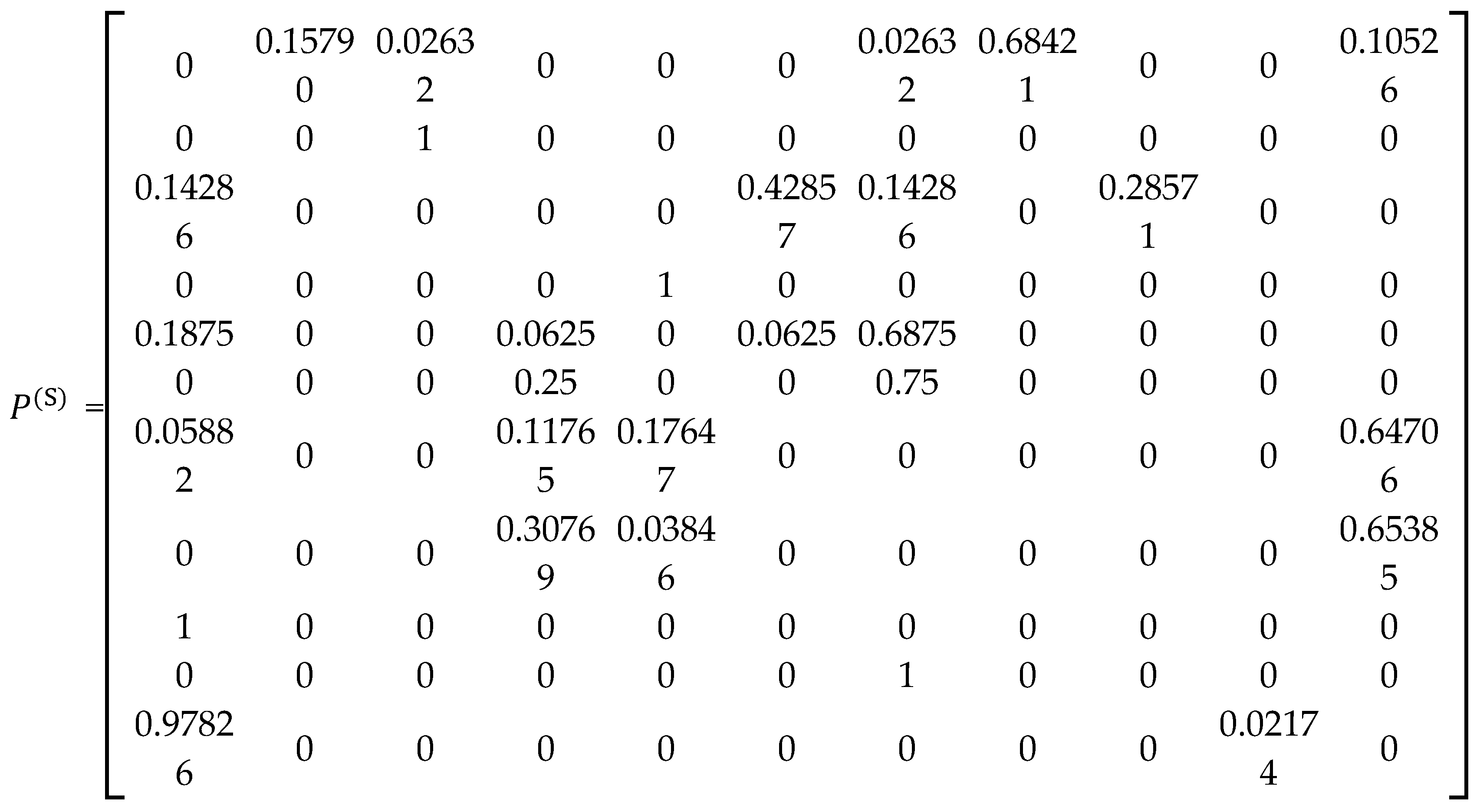
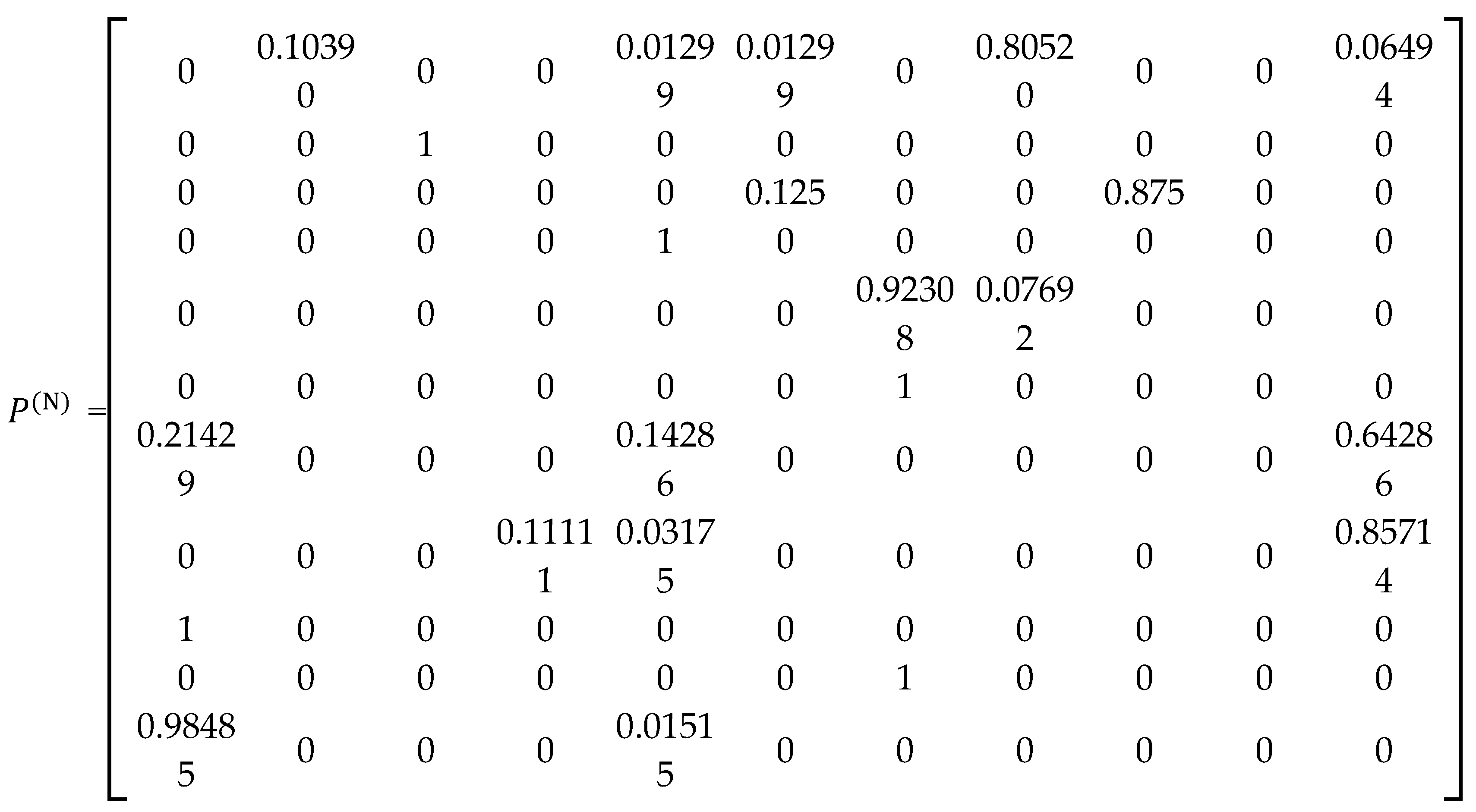
Two groups of vehicles, conventionally named “New” and “Old”, were randomly selected for the analysis. The estimation results obtained are summarised in Table 3 and in matrices (22) and (23). They form the basis for carrying out the simulation experiment.
The transition matrix for the subset of “Old” buses P(S) has the form:
The transition matrix for the subset of “New” buses P(N) has the form:
The global economic efficiency indicator ZSK, i.e. the profit from the operation of the vehicles (the mean value of the random sequence zr[j]), is determined in conventional units. The data necessary for its calculation are hypothetical and, owing to the lack of real data, serve as an illustration of the considerations.
In order to verify the hypothesis concerning the influence of the length of the period of operation of the buses on the efficiency of the operation and maintenance process carried out in the urban public transport system, simulation runs of the operation and maintenance process were performed for the following combinations of input parameters:
- the transition matrix and the values of the parameters of the sojourn time distributions in the states for the set of “New” buses,
- the transition matrix and the values of the parameters of the sojourn time distributions in the states for the set of “Old” buses,
- the transition matrix for the set of “New” buses and the values of the parameters of the sojourn time distributions in the states for the set of “Old” buses,
- the transition matrix for the set of “Old” buses and the values of the parameters of the sojourn time distributions in the states for the set of “New” buses.
These results confirm the influence of the length of the buses’ period of operation on the efficiency of the operation and maintenance process. For the examined subsets of buses, it was observed that the values of the elements of the transition probability matrix had a greater influence on the value of the mean total sojourn time in state S1 than the values of the parameters of the distributions of sojourn times in the states.
Moreover, on the basis of an analysis of the values of the statistics of mean absolute deviation d and skewness g presented in Table 4, Table 5, Table 6 and Table 7, it can be concluded that the sums of the sojourn times in the distinguished states of the operation and maintenance process are normally distributed. Under the hypothesis of normality of the distribution, the values of statistic d (mean absolute deviation) should lie in the interval (0.7692, 0.8322), and those of statistic g (skewness) in the interval (-0.430, 0.430), at the confidence level 1-α = 0.02 for n = 200.
To examine the influence of the mean value of the sojourn time in state S1 on the efficiency of the operation and maintenance process, simulation runs were carried out for k = 11 different mean values of the sojourn time in state S1. The value of ET1 successively ranged from 11.05 (the value corresponding to the set of “Old” buses) to 13.05 (the value corresponding to the set of “New” buses) in steps of 0.2. The simulation runs were performed with the remaining input parameter values corresponding both to the set of “New” buses and to the set of “Old” buses. The results of the experiment are summarised in Table 8 and Table 9. They confirm the influence of the mean value of the sojourn time in state S1 on the efficiency of the operation and maintenance process.
All simulation runs of the operation and maintenance process were carried out with the following remaining input data for the simulation program:
- type of distribution of the vehicles’ sojourn times in the individual states – gamma distribution,
- number of objects – n = 200 buses,
- modelling time – tk = 1000 h.
The results obtained are qualitatively consistent with the results of studies of urban public transport buses operated under real conditions. In the experiments conducted, the mean total sojourn time in state S1 over a modelling time of 1000 h was 681.1 h for the subset of “New” buses and 514.0 h for the “Old” subset, and the profit ZSK was 113.6 and 31.8 conventional units, respectively. Increasing ET1 from 11.05 h to 13.05 h increased ZSK from 32.78 to 47.01 for the “Old” subset and from 102.87 to 113.65 for the “New” subset; the difference between the subsets therefore stems to a greater extent from the remaining parameters of the model – the transition matrix and the parameters of the sojourn time distributions (except for ET1) – than from the value of ET1 itself. This justifies the use, as in [14,16,17], of evaluation criteria (availability, profit per unit time) determined for the entire operation and maintenance process, taking into account the states of renewal, diagnosing and waiting, rather than solely the time spent carrying out transport tasks. The ZSK values are illustrative, since the data on unit revenues and expenditures are hypothetical; these data can be made realistic by means of the method for the preliminary estimation of unit costs presented in [5]. The assumption of a gamma distribution for all states is a simplification – in [19], the sojourn time distributions were selected separately for the individual states, and the simulation results were verified against the semi-Markov model (the relative differences did not exceed 6%). An analogous comparison of the simulation results with the limiting values determined from Equations (8) and (16) is a natural direction for further verification of the presented model.
7. Conclusions
At the current stage of development of the model, the main objective was to verify the results generated in the simulation process for two groups of buses with significantly different operational parameters, i.e. for the groups of “Old” and “New” buses. The share of the total simulation time accounted for by driving time was adopted as the evaluation indicator. Observational data and data obtained from studies of the operation and maintenance process show that this indicator has a higher value for new buses. This means that the results obtained from the study of the simulation model are consistent with the real-world results.
For the examined subsets of buses, it was observed that the values of the elements of the transition probability matrix had a greater influence on the value of the mean total sojourn time in state S1 than the values of the parameters of the distributions of sojourn times in the states.
On the basis of the results of operational tests of reference (ideal) objects, expert opinions and the results of simulations of the operation and maintenance process, criterion values of the indicators describing the model can be determined. These values enable comparison with the real process. Comparing the results of calculations obtained from studies of the real transport system with the criterion values constitutes an assessment of the efficiency of its functioning.
The considerations presented in this paper concern the operation and maintenance system of urban public transport buses. However, owing to the assumed degree of generality of the description, they can be used to analyse the operation and maintenance process carried out in other systems with a similar structure and objective function.
References
- Moore P.G.: Introduction to Operations Research (In Polish). WNT, Warsaw 1973.
- Fishman G.S.: Computer Simulation: Concepts and Methods (In Polish). PWE, Warsaw 1981.
- Zeigler B.P.: Theory of Modelling and Simulation (In Polish). PWN, Warsaw 1984.
- Woropay M., Knopik L., Landowski B.: Modelling of Operation and Maintenance Processes in a Transport System (In Polish). Biblioteka Problemów Eksploatacji, Wydawnictwo Instytutu Technologii Eksploatacji, Bydgoszcz–Radom 2001.
- Landowski B., Muślewski Ł., Pająk M., Polishchuk O.: Method for initial assessment of unit costs of public city transport means operation. MATEC Web of Conferences, 2018, 182, 01010. [CrossRef]
- Grabski F.: Semi-Markov Processes: Applications in System Reliability and Maintenance. Elsevier 2015. [CrossRef]
- Woropay M., Grzegórski J., Landowski B.: Simulation model of the operation and maintenance of a certain class of technical objects (In Polish). Zeszyty Naukowe AGH: Mechanika, 1994, 13(3).
- Woropay M., Grzegórski J., Landowski B.: Decision variables for the modernisation of an operation and maintenance system (In Polish). In: 3rd National and 2nd International Scientific Conference “Development of Theory and Technology in the Technical Modernisation of Agriculture”. Wydawnictwa Naukowe ART, Olsztyn 1994.
- Woropay M., Knopik L., Landowski B.: Simulation model for optimising the process of achieving the goals of an operation and maintenance system (In Polish). In: 7th Scientific Conference “Problems of the Development of Working Machines”, Warsaw–Wrocław–Stalowa Wola–Zakopane, January 1994. MCNEMT, Radom 1994, 289–298.
- Woropay M., Knopik L., Landowski B.: Influence of changes in the value of a selected control variable on the efficiency of the operation and maintenance process of technical systems (In Polish). In: 4th International Seminar “Efficiency of the Operation of Technical Systems”, Olsztyn, 24–26 April 1997. ART, Olsztyn 1997.
- Woropay M., Landowski B.: Simulation analysis of the operation and maintenance process in an urban public transport system (In Polish). Zeszyty Naukowe ATR w Bydgoszczy No. 212, Mechanika 42. Wydawnictwo Uczelniane ATR, Bydgoszcz 1998.
- Landowski B., Woropay M., Neubauer A.: Reliability Control in Transport Systems (In Polish). Biblioteka Problemów Eksploatacji, Wydawnictwo Instytutu Technologii Eksploatacji, Bydgoszcz–Radom 2004.
- Landowski B.: Numerical simulation of the process of a technical object state changes. Journal of KONBiN, 2017, 44(1), 119–140. [CrossRef]
- Migawa K., Neubauer A., Muślewski Ł., Landowski B.: Method of availability control in the transport system using simulation model of operation and maintenance process. Journal of KONBiN, 2017, 44(1), 59–79. [CrossRef]
- Landowski B.: Method of modelling operation and maintenance processes in public transport systems using a certain class of stochastic processes. MATEC Web of Conferences, 2021, 332, 01005. [CrossRef]
- Knopik L., Migawa K.: Semi-Markov system model for minimal repair maintenance. Eksploatacja i Niezawodność – Maintenance and Reliability, 2019, 21(2), 256–260. [CrossRef]
- Migawa K., Borowski S., Neubauer A., Sołtysiak A.: Semi-Markov model of the system of repairs and preventive replacements by age of city buses. Applied Sciences, 2021, 11(21), 10411. [CrossRef]
- Kozłowski E., Borucka A., Świderski A.: Application of the logistic regression for determining transition probability matrix of operating states in the transport systems. Eksploatacja i Niezawodność – Maintenance and Reliability, 2020, 22(2), 192–200. [CrossRef]
- Oszczypała M., Ziółkowski J., Małachowski J.: Modelling the operation process of light utility vehicles in transport systems using Monte Carlo simulation and semi-Markov approach. Energies, 2023, 16(5), 2210. [CrossRef]
- Zio E.: The Monte Carlo Simulation Method for System Reliability and Risk Analysis. Springer, London 2013. [CrossRef]
- Rymarz J., Niewczas A., Krzyżak A.: Comparison of operational availability of public city buses by analysis of variance. Eksploatacja i Niezawodność – Maintenance and Reliability, 2016, 18(3), 373–378. [CrossRef]
- Niewczas A., Rymarz J., Ślęzak M., Kasperek D., Hołyszko P.: Reliability study of electric buses in the urban public transport system. Energies, 2025, 18(14), 3863. [CrossRef]
- Silvestrov D.: Coupling and Ergodic Theorems for Semi-Markov-Type Processes I. Springer, Cham 2025. [CrossRef]
- Limnios N., Swishchuk A.: Discrete-Time Semi-Markov Random Evolutions and Their Applications. Probability and Its Applications. Springer, Cham 2023. [CrossRef]
- Wu B., Garcia Maya B.I., Limnios N.: Using semi-Markov chains to solve semi-Markov processes. Methodology and Computing in Applied Probability, 2021, 23(4), 1419–1431. [CrossRef]
- Mokhtari F., Ayhar C., Barbu V.S., Rahmani S.: Kernel estimators of Markov renewal and semi-Markov transition functions of semi-Markov systems. Journal of Nonparametric Statistics, 2026, 38(2), 421–444. [CrossRef]
- Grabski F.: Non-homogeneous four state semi-Markov reliability model of operation process. In: Theory and Applications of Dependable Computer Systems. Advances in Intelligent Systems and Computing. Springer, Cham 2020, 252–262. [CrossRef]
- Oszczypała M., Ziółkowski J., Małachowski J.: Semi-Markov approach for reliability modelling of light utility vehicles. Eksploatacja i Niezawodność – Maintenance and Reliability, 2023, 25(2), 161859. [CrossRef]
- Szczuka A., Zieliński R.: Generators of gamma-distributed random numbers (In Polish). Roczniki PTM, Seria III: Matematyka Stosowana, 1993, XXXVI.
- Silvestrov D.S.: Semi-Markov Processes with a Discrete State Space (In Russian). Sovetskoe Radio, Moscow 1980.
- Grabski F.: On a certain problem of the optimisation of preventive servicing (In Polish). Zagadnienia Eksploatacji Maszyn, 1985, 2(62).
- Zieliński R.: Random Number Generators (In Polish). WNT, Warsaw 1979.
- Greń J.: Mathematical Statistics: Models and Problems (In Polish). PWN, Warsaw 1974.
Figure 1.
Directed graph of the process states.
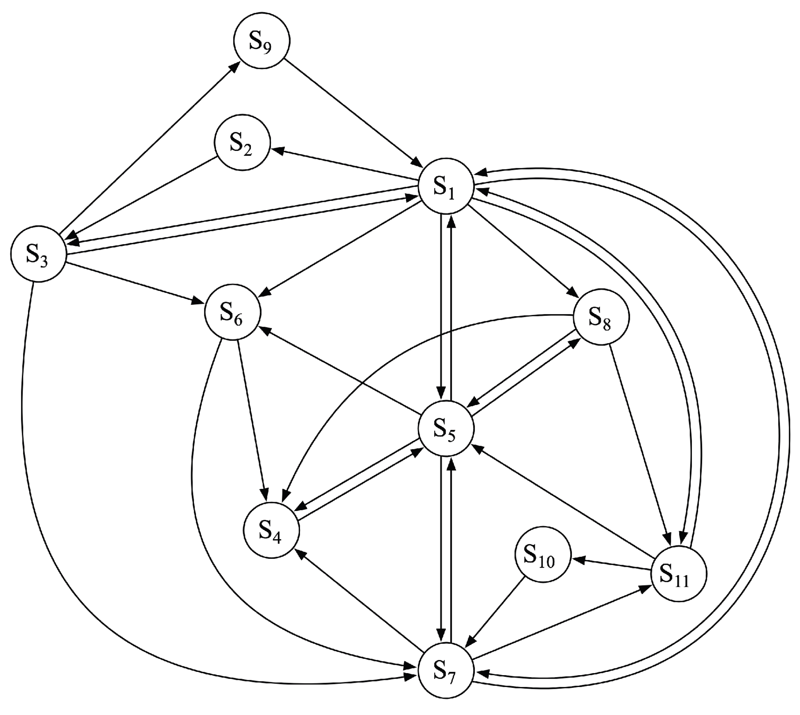

Table 1.
Parameters of the sojourn times in the states.
| State | Mean sojourn time in the i-th state | Standard deviation |
|---|---|---|
| S1 (Old) | 2.5 days | 0.7 days |
| S1 (New) | 3.3 days | 0.7 days |
| S2 | 20 min | 10 min |
| S3 | 53 min | 35 min |
| S4 | 30 min | 10 min |
| S5 | 77 min | 50 min |
| S6 | 10 min | 3 min |
| S7 | 15 min | 5 min |
| S8 | 15 min | 5 min |
| S9 | 60 min | 20 min |
| S10 | 50 min | 30 min |
| S11 | 60 min | 20 min |
Table 2.
Selected results of the simulation studies.
| Run 1 | Run 2 | Run 3 | Run 4 | Run 5 | ||||||
|---|---|---|---|---|---|---|---|---|---|---|
| Indicator | Old | New | Old | New | Old | New | Old | New | Old | New |
| Number of failures | 37.91 | 29.95 | 38.08 | 30.33 | 37.80 | 29.96 | 38.18 | 29.95 | 37.90 | 29.87 |
| % of driving time | 92.91 | 94.53 | 92.89 | 94.44 | 92.85 | 94.13 | 93.19 | 94.37 | 92.73 | 94.45 |
Table 3.
Data characterising the individual states.
| Process state | S1 | S2 | S3 | S4 | S5 | S6 | S7 | S8 | S9 | S10 | S11 |
|---|---|---|---|---|---|---|---|---|---|---|---|
| Sojourn time in the state [h] | |||||||||||
| Subset of “Old” buses | |||||||||||
| Mean X | 11.05 | 0.20 | 0.43 | 2.93 | 3.53 | 0.13 | 0.25 | 0.08 | 0.25 | 2.25 | 9.02 |
| Standard deviation | 5.08 | 0.06 | 0.20 | 0.67 | 0.56 | 0.05 | 0.11 | 0.02 | 0.16 | 0.80 | 1.61 |
| Subset of “New” buses | |||||||||||
| Mean X | 13.05 | 0.08 | 0.38 | 2.15 | 2.43 | 0.12 | 0.20 | 0.08 | 0.26 | 2.25 | 6.03 |
| Standard deviation | 1.11 | 0.06 | 0.20 | 0.25 | 0.45 | 0.05 | 0.11 | 0.02 | 0.16 | 0.80 | 0.62 |
| Revenue (expenditure) per unit time | |||||||||||
| Unit profit z[j] | 200 | −5 | −5 | −5 | −1000 | −5 | −5 | −40 | −5 | −5 | −5 |
Table 4.
Results of the simulation experiments – values of selected statistics of the total sojourn time in the states and of the unit profit for the input parameter values of the “New” buses.
Table 4.
Results of the simulation experiments – values of selected statistics of the total sojourn time in the states and of the unit profit for the input parameter values of the “New” buses.
| State of the operation and maintenance process | ||||||||||||
|---|---|---|---|---|---|---|---|---|---|---|---|---|
| Parameter | S1 | S2 | S3 | S4 | S5 | S6 | S7 | S8 | S9 | S10 | S11 | ZSK |
| Mean | 681.1 | 0.4 | 2.1 | 9.9 | 21.0 | 0.2 | 1.8 | 3.4 | 1.3 | 0 | 273.4 | 113.6 |
| Standard deviation | 12.6 | 0.2 | 0.9 | 4.2 | 7.6 | 0.2 | 0.7 | 0.2 | 0.6 | 0 | 11.3 | 9.3 |
| Coefficient of variation | 0.018 | 0.478 | 0.433 | 0.423 | 0.362 | 0.937 | 0.398 | 0.068 | 0.456 | 0 | 0.041 | 0.082 |
| MIN | 642.5 | 0.0 | 0.0 | 0.0 | 3.4 | 0.0 | 0.3 | 2.6 | 0.0 | 0 | 240.1 | 82.9 |
| MAX | 709.7 | 1.1 | 4.5 | 22.2 | 43.9 | 0.9 | 4.7 | 4.0 | 3.2 | 0 | 310.2 | 134.4 |
| Absolute deviation | 0.8 | 0.81 | 0.8 | 0.8 | 0.79 | 0.76 | 0.79 | 0.8 | 0.79 | 0 | 0.78 | 0.79 |
| Skewness | −0.24 | 0.45 | 0.51 | 0.12 | 0.11 | 1.43 | 0.68 | −0.01 | 0.54 | 0 | 0.09 | −0.22 |
Table 5.
Results of the simulation experiments – values of selected statistics of the total sojourn time in the states and of the unit profit for the input parameter values of the “Old” buses.
Table 5.
Results of the simulation experiments – values of selected statistics of the total sojourn time in the states and of the unit profit for the input parameter values of the “Old” buses.
| State of the operation and maintenance process | ||||||||||||
|---|---|---|---|---|---|---|---|---|---|---|---|---|
| Parameter | S1 | S2 | S3 | S4 | S5 | S6 | S7 | S8 | S9 | S10 | S11 | ZSK |
| Mean | 514.0 | 1.5 | 3.7 | 47.1 | 68.8 | 0.6 | 5.2 | 2.6 | 0.6 | 2.6 | 353.3 | 31.8 |
| Standard deviation | 8.2 | 0.2 | 0.4 | 4.2 | 5.3 | 0.1 | 0.4 | 0.1 | 0.1 | 0.8 | 7.8 | 6.4 |
| Coefficient of variation | 0.016 | 0.116 | 0.114 | 0.089 | 0.077 | 0.153 | 0.074 | 0.032 | 0.224 | 0.307 | 0.022 | 0.201 |
| MIN | 495.1 | 0.9 | 2.5 | 35.4 | 56.0 | 0.4 | 4.2 | 2.4 | 0.3 | 0.5 | 331.7 | 16.2 |
| MAX | 536.0 | 1.9 | 4.7 | 61.8 | 81.8 | 0.9 | 6.3 | 2.8 | 1.0 | 6.2 | 375.6 | 47.8 |
| Absolute deviation | 0.83 | 0.79 | 0.81 | 0.77 | 0.78 | 0.81 | 0.78 | 0.8 | 0.8 | 0.77 | 0.79 | 0.78 |
| Skewness | −0.1 | −0.04 | −0.19 | 0.23 | 0.08 | 0.23 | 0.08 | 0.02 | 0.19 | 0.5 | 0.14 | −0.08 |
Table 6.
Results of the simulation experiments – values of selected statistics of the total sojourn time in the states and of the unit profit for the transition matrix of the “New” buses and the sojourn time distributions of the “Old” buses.
Table 6.
Results of the simulation experiments – values of selected statistics of the total sojourn time in the states and of the unit profit for the transition matrix of the “New” buses and the sojourn time distributions of the “Old” buses.
| State of the operation and maintenance process | ||||||||||||
|---|---|---|---|---|---|---|---|---|---|---|---|---|
| Parameter | S1 | S2 | S3 | S4 | S5 | S6 | S7 | S8 | S9 | S10 | S11 | ZSK |
| Mean | 554.8 | 1.1 | 2.3 | 13.2 | 29.3 | 0.2 | 2.2 | 3.2 | 1.1 | 0 | 392.3 | 79.5 |
| Standard deviation | 22.6 | 0.5 | 1.0 | 6.4 | 11.1 | 0.1 | 0.8 | 0.3 | 0.6 | 0 | 21.5 | 13.9 |
| Coefficient of variation | 0.041 | 0.438 | 0.427 | 0.486 | 0.379 | 0.887 | 0.371 | 0.080 | 0.540 | 0 | 0.055 | 0.175 |
| MIN | 491.3 | 0.0 | 0.0 | 0.0 | 4.1 | 0.0 | 0.4 | 2.6 | 0.0 | 0 | 309.3 | 36.3 |
| MAX | 606.2 | 2.6 | 4.5 | 32.8 | 60.5 | 0.7 | 4.4 | 3.8 | 3.3 | 0 | 446.2 | 109.6 |
| Absolute deviation | 0.79 | 0.8 | 0.84 | 0.81 | 0.81 | 0.8 | 0.81 | 0.81 | 0.8 | 0 | 0.8 | 0.8 |
| Skewness | −0.21 | 0.3 | 0.04 | 0.2 | 0.25 | 0.78 | 0.19 | −0.34 | 0.52 | 0 | −0.25 | −0.32 |
Table 7.
Results of the simulation experiments – values of selected statistics of the total sojourn time in the states and of the unit profit for the transition matrix of the “Old” buses and the sojourn time distributions of the “New” buses.
Table 7.
Results of the simulation experiments – values of selected statistics of the total sojourn time in the states and of the unit profit for the transition matrix of the “Old” buses and the sojourn time distributions of the “New” buses.
| State of the operation and maintenance process | ||||||||||||
|---|---|---|---|---|---|---|---|---|---|---|---|---|
| Parameter | S1 | S2 | S3 | S4 | S5 | S6 | S7 | S8 | S9 | S10 | S11 | ZSK |
| Mean | 643.7 | 0.6 | 3.5 | 37.5 | 51.0 | 0.6 | 4.5 | 2.6 | 0.7 | 3.0 | 246.6 | 76.2 |
| Standard deviation | 18.9 | 0.3 | 1.3 | 9.7 | 12.5 | 0.3 | 1.1 | 0.3 | 0.5 | 2.7 | 16.8 | 15.0 |
| Coefficient of variation | 0.029 | 0.456 | 0.359 | 0.258 | 0.245 | 0.473 | 0.240 | 0.105 | 0.763 | 0.919 | 0.068 | 0.197 |
| MIN | 581.9 | 0.1 | 0.6 | 15.1 | 19.7 | 0.0 | 2.2 | 1.9 | 0.0 | 0.0 | 199.7 | 22.0 |
| MAX | 697.1 | 1.8 | 7.9 | 62.0 | 92.7 | 1.6 | 8.0 | 3.4 | 2.9 | 12.7 | 297.1 | 106.3 |
| Absolute deviation | 0.8 | 0.78 | 0.8 | 0.79 | 0.79 | 0.79 | 0.83 | 0.8 | 0.8 | 0.81 | 0.77 | 0.8 |
| Skewness | −0.14 | 0.7 | 0.41 | 0.25 | 0.37 | 0.54 | 0.36 | −0.03 | 0.89 | 0.85 | 0.24 | −0.48 |
Table 8.
Total sojourn time in the individual states and profit from the operation of the vehicles for the subset of “Old” buses depending on ET1.
Table 8.
Total sojourn time in the individual states and profit from the operation of the vehicles for the subset of “Old” buses depending on ET1.
| State of the operation and maintenance process | ||||||||||||
|---|---|---|---|---|---|---|---|---|---|---|---|---|
| ET1 | S1 | S2 | S3 | S4 | S5 | S6 | S7 | S8 | S9 | S10 | S11 | ZSK |
| 11.05 | 516.69 | 1.47 | 3.66 | 47.6 | 68.86 | 0.62 | 5.15 | 2.55 | 0.61 | 2.75 | 349.93 | 32.78 |
| 11.25 | 524.29 | 1.46 | 3.69 | 45.38 | 65.67 | 0.64 | 4.99 | 2.52 | 0.62 | 2.82 | 347.77 | 35.22 |
| 11.45 | 525.36 | 1.46 | 3.62 | 46.73 | 67.46 | 0.63 | 4.94 | 2.49 | 0.63 | 2.5 | 343.95 | 35.99 |
| 11.65 | 529.88 | 1.38 | 3.46 | 46.89 | 69.16 | 0.61 | 5.08 | 2.49 | 0.55 | 2.85 | 337.34 | 37.53 |
| 11.85 | 537.71 | 1.43 | 3.57 | 43.47 | 63.49 | 0.58 | 4.85 | 2.44 | 0.56 | 2.85 | 338.7 | 40.64 |
| 12.05 | 541.55 | 1.42 | 3.55 | 44.93 | 65.19 | 0.63 | 4.74 | 2.44 | 0.56 | 2.14 | 332.42 | 41.54 |
| 12.25 | 541.1 | 1.36 | 3.3 | 43.69 | 63.79 | 0.57 | 4.78 | 2.44 | 0.57 | 2.59 | 335.27 | 42.96 |
| 12.45 | 546.82 | 1.44 | 3.58 | 43.07 | 64.03 | 0.61 | 4.81 | 2.36 | 0.62 | 2.35 | 329.79 | 43.76 |
| 12.65 | 546.47 | 1.29 | 3.26 | 44.74 | 65.67 | 0.6 | 4.79 | 2.4 | 0.57 | 2.55 | 327.03 | 45.08 |
| 12.85 | 553.17 | 1.28 | 3.18 | 43.17 | 63.9 | 0.56 | 4.79 | 2.34 | 0.51 | 2.76 | 323.71 | 45.3 |
| 13.05 | 557.61 | 1.36 | 3.36 | 42.95 | 63.05 | 0.59 | 4.67 | 2.31 | 0.55 | 2.3 | 320.56 | 47.01 |
Table 9.
Total sojourn time in the individual states and profit from the operation of the vehicles for the subset of “New” buses depending on ET1.
Table 9.
Total sojourn time in the individual states and profit from the operation of the vehicles for the subset of “New” buses depending on ET1.
| State of the operation and maintenance process | ||||||||||||
|---|---|---|---|---|---|---|---|---|---|---|---|---|
| ET1 | S1 | S2 | S3 | S4 | S5 | S6 | S7 | S8 | S9 | S10 | S11 | ZSK |
| 11.05 | 642.77 | 0.45 | 2.15 | 11.52 | 23.95 | 0.19 | 2.13 | 3.79 | 1.27 | 0 | 307.84 | 102.87 |
| 11.25 | 647.64 | 0.47 | 2.22 | 11.03 | 22.97 | 0.18 | 2.02 | 3.73 | 1.35 | 0 | 304.6 | 104.85 |
| 11.45 | 652.55 | 0.46 | 2.09 | 10.98 | 23.19 | 0.19 | 2.06 | 3.69 | 1.33 | 0 | 299.52 | 105.65 |
| 11.65 | 658.21 | 0.48 | 2.36 | 10.5 | 21.79 | 0.18 | 1.91 | 3.63 | 1.4 | 0 | 295.45 | 106.21 |
| 11.85 | 659.3 | 0.47 | 2.24 | 10.28 | 22.28 | 0.17 | 2.02 | 3.57 | 1.32 | 0 | 293.57 | 107.91 |
| 12.05 | 663 | 0.45 | 2.08 | 10.29 | 22.17 | 0.16 | 1.98 | 3.59 | 1.24 | 0 | 290.69 | 108.82 |
| 12.25 | 667.28 | 0.48 | 2.16 | 11.27 | 22.53 | 0.16 | 1.96 | 3.5 | 1.33 | 0 | 285.06 | 109.33 |
| 12.45 | 670.1 | 0.46 | 2.06 | 10.42 | 22.02 | 0.16 | 1.92 | 3.49 | 1.26 | 0 | 283.02 | 110.4 |
| 12.65 | 673.97 | 0.43 | 2.08 | 9.97 | 21.61 | 0.16 | 1.94 | 3.42 | 1.24 | 0 | 280.26 | 111.62 |
| 12.85 | 676.76 | 0.42 | 2.07 | 10.11 | 20.81 | 0.16 | 1.84 | 3.43 | 1.24 | 0 | 277.97 | 112.97 |
| 13.05 | 681.11 | 0.43 | 2.1 | 9.94 | 21.03 | 0.17 | 1.84 | 3.35 | 1.27 | 0 | 273.41 | 113.65 |
Disclaimer/Publisher’s Note: The statements, opinions and data contained in all publications are solely those of the individual author(s) and contributor(s) and not of MDPI and/or the editor(s). MDPI and/or the editor(s) disclaim responsibility for any injury to people or property resulting from any ideas, methods, instructions or products referred to in the content. |
© 2026 by the authors. Licensee MDPI, Basel, Switzerland. This article is an open access article distributed under the terms and conditions of the Creative Commons Attribution (CC BY) license (http://creativecommons.org/licenses/by/4.0/).
Copyright: This open access article is published under a Creative Commons CC BY 4.0 license, which permit the free download, distribution, and reuse, provided that the author and preprint are cited in any reuse.