
Submitted:
17 November 2026
Posted:
18 November 2026
You are already at the latest version
Abstract
Cognitive cities need weather intelligence that supports decisions, yet AI weather models are mostly judged by forecast error. We propose a climate-intelligence framework that links probabilistic AI forecasts to activity-specific urban decisions and implement its decision layer. The 51 ECMWF AIFS ENS members are bias-corrected using only past forecasts of the same model version and converted into a probability of extreme heat; each activity acts when this probability exceeds its scenario cost/loss ratio. The layer is evaluated at twelve Saudi cognitive-city sites (ten independent series) over the 2025 and 2026 hot seasons against ERA5 and airport observations. Bias-corrected probabilities reached Brier skill scores of 0.45–0.59. They raised relative economic value by 0.19–0.22 over uncorrected ensemble-mean warnings (p ≤ 0.003), by 0.13–0.24 over a bias-corrected ensemble-mean warning (one-sided p ≤ 0.02) and by 0.08–0.10 over a deterministic rule tuned to each activity (not significant in a two-sided test). For low-cost protective decisions (cost/loss ratios of 0.05–0.10), probabilities exceeded both of these rules by 0.21–0.83 (p ≤ 0.006). Against ten airports the ranking held with lower value, and skill was negative at two coastal stations. The value of AI forecasts for a cognitive city therefore lies in a local, bias-corrected decision layer, and shared probabilities matter most for the low-cost actions that protect people.
Keywords:
cognitive cities
; climate intelligence
; AI weather prediction
; ensemble forecasting
; decision value
; cost/loss model
; extreme heat
; urban resilience
; decision support
; Saudi Arabia
1. Introduction
The value of an AI weather forecast to a city lies in the decisions it changes, not in its error statistics alone. Machine-learning weather prediction (MLWP) models such as GraphCast and Pangu-Weather now match or exceed physics-based systems at a fraction of the computing cost [1,2], and the European Centre for Medium-Range Weather Forecasts (ECMWF) runs its Artificial Intelligence Forecasting System (AIFS) operationally [3]. Ensemble versions, such as the 51-member AIFS ENS, add the uncertainty information that risk-sensitive operations need [4,5].
Cognitive cities are meant to turn such information into action. Smart-city research has long framed urban intelligence as the coupling of data, models and decision support [6], and AI is now applied across urban energy, health, mobility and environmental management [7]. Cognitive cities go a step further: where smart cities emphasise control and efficiency, cognitive cities are expected to learn from experience and to adapt to disruption [8,9]. Saudi Arabia is building several, from NEOM to research and innovation campuses such as KAUST and KACST, in one of the hottest climates on Earth, where extreme heat is projected to approach the limits of human adaptability [10], urban heat stress is rising [11] and mass gatherings are increasingly exposed [12]. Yet a heat forecast means different things to a hospital, an outdoor work site, a power operator and an events team. Each has its own cost of acting and its own loss from not acting.
Most MLWP studies stop at verification against reanalysis [13], and most smart-city work treats the forecast as a given input. Recent work has begun to value AI forecasts for cities with the cost/loss model, but with deterministic forecasts and one user per city [14]. How forecast probabilities should be turned into activity-specific action within a city has not been tested. Our earlier work corrected GraphCast-family forecasts over Saudi Arabia, quantified their uncertainty and generated city bulletins with a language model [15]; it did not test whether uncertainty-aware forecasts lead to better decisions.
This paper addresses that gap. Its contributions are as follows:
- A climate-intelligence framework for cognitive cities that separates forecast, probability, urban-context and decision layers, and states which layer each method serves;
- An implemented decision layer that applies real-time, version-aware bias correction to AIFS ENS members and maps heat probabilities to activity-specific action thresholds at twelve Saudi cognitive-city sites and innovation nodes;
- A test of that layer against deterministic baselines, including a rule tuned to each activity, using relative economic value, probabilistic skill and event metrics, a block bootstrap and verification against airport observations;
- Evidence on which component creates value for which urban activity, and where probabilities do not outperform simpler rules.
The research questions are: (RQ1) how skilful and reliable are bias-corrected AIFS ENS heat probabilities at Saudi cognitive-city sites at lead times of two to six days; (RQ2) do probability-based decisions give higher relative economic value than deterministic decisions; and (RQ3) how does that value differ across urban activities with different cost/loss profiles?
2. Related Work
2.1. AI Weather Models and Their Ensembles
GraphCast showed that a graph neural network trained on ERA5 can outperform ECMWF HRES on most verification targets [1]. Probabilistic successors such as GenCast [5] and the CRPS-trained AIFS ensemble [4] now outperform the physics-based ECMWF ensemble for most variables and lead times in the medium range. AIFS ENS became operational on 1 July 2025 with 51 members and is distributed openly [16]; version 2 replaced version 1 from the 06 UTC run of 12 May 2026 [17]. Its skill, however, has been reported mainly as global or European scores [4,13].
2.2. Limits of AI Forecasts for Heat
AI models are least reliable where cities need them most. GraphCast and Pangu-Weather show cold biases before and during heatwaves [18]. For record-breaking heat, cold and wind, ECMWF HRES outperforms GraphCast, Pangu-Weather and FuXi at almost all lead times, and the AI models underestimate both the intensity and the frequency of records [19]. The picture is not uniform: for near-surface extremes, the relative skill of data-driven and physics-based models varies with region, type of extreme and lead time [20]. In the Middle East, four deterministic AI models captured the timing and persistence of the June 2024 compound heatwave but underestimated its daytime peaks [21]; that evaluation, like most, measured forecast error and did not address probabilistic forecasts or decisions. Over Saudi Arabia, our earlier work found a systematic cold bias in GraphCast-family 2 m temperature [15]. These findings motivate two choices here: a local bias-correction step, and evaluating decisions rather than assuming the forecast is correct.
2.3. From Forecast Skill to Decision Value
The cost/loss model values a forecast by how much it saves a user who pays a cost C to protect against a loss L [22,23]. Probabilities from an ensemble yield more value than a deterministic forecast from the same model because each user can act at their own probability threshold [23,24], and the value realised depends on the user’s cost/loss ratio as well as on forecast skill [25]. Two recent studies bring this logic to AI forecasts. Olivetti et al. extend relative economic value with varying cost/loss ratios and penalties for compounding misses and repeated false alarms, and compare physics-based IFS HRES with deterministic AIFS for cities exposed to extremes; the better model changes with the cost/loss ratio [14]. Aitken et al. show with decision theory that a calibrated probabilistic forecast serves users with different constraints better than a deterministic message, and apply it to AI monsoon forecasts for farmers in India [26].
2.4. Heat Early Warning and Urban Decisions
Operational heat warnings still rely mostly on fixed thresholds and colour codes, which are weakly tied to the decisions of local authorities, health services and employers [27,28]. Two lines of work try to close this gap. Impact forecasting extends hazard forecasts with estimates of their consequences so that emergency managers can act on them [29], and forecast-based financing matches threshold forecast probabilities with pre-agreed actions [30]. For heat specifically, extended-range ensemble forecasts of heatwave days over Europe have been verified probabilistically [31] and translated into alert levels with rule-based logic [32]. In Saudi Arabia, outdoor construction workers face excessive heat stress for most of the summer workday, and the midday outdoor work ban does not remove that risk [33].
2.5. Cognitive Cities and Climate Intelligence
Agentic and digital-twin frameworks link sensing, forecasting and emergency response in climate-resilient cities [34,35], and integrated AI is argued to be central to early warning of compound climate risk [36]. Urban digital twins already combine real-time weather data with simulation to assess outdoor thermal comfort at campus scale [37]. Research on Saudi cognitive cities themselves has so far been largely conceptual and qualitative, for example interpretive and critical case studies of NEOM and THE LINE [38,39]; we found few quantitative evaluations of the services that such cities would operate. These frameworks treat the forecast, where they use one, as an input and do not measure the value of acting on it. Table 1 positions this paper against the closest studies.
We found no study that measures the decision value of AI ensemble heat probabilities for different activities within cognitive cities, or for a hyper-arid climate. The methodological basis, relative economic value, is well established [14,23]; the novelty of this paper lies in the probabilistic input from a newly operational AI ensemble, the heterogeneity of activities within a city, the comparison against activity-tuned deterministic rules, and the region.
3. Materials and Methods
3.1. Climate-Intelligence Framework
The framework has five layers (Figure 1). The AI forecast layer is used as delivered, so the contribution lies in how forecast uncertainty and urban context become decisions, not in weather modelling. This study implements the probability, cognitive-city context and decision layers and evaluates the decision layer. The operations layer, where alerts and bulletins such as those of the language-model agent in our earlier work [15] would sit, is designed but not evaluated here.
3.2. Data
Forecasts. ECMWF AIFS ENS forecasts were taken from the ECMWF open-data archive [16], read from its public mirror on Google Cloud Storage: the control and 50 perturbed members at 0.25°, from 00 UTC runs. We used 2 m temperature at lead times of +36 h, +84 h and +132 h (days 2, 4 and 6), all valid at 12 UTC (15:00 local time, near the daily maximum). Initialisation dates cover 2 July–30 September 2025 and 1 May–30 September 2026, giving 244 initialisations per site and lead time, or 732 forecasts per site; the 1 July 2025 run is missing from the archive. The period therefore covers all hot-season months (May–September) available since AIFS ENS became operational. Because version 2 started with the 06 UTC run of 12 May 2026, the 00 UTC runs up to 12 May 2026 come from AIFS ENS version 1 and those from 13 May 2026 from version 2 [17]; the runs of 12 and 13 May, at the changeover, were checked and showed no anomaly, so none were excluded. Only the 2 m temperature messages were read from each file, and the nearest grid point to each site was extracted using the coordinates stored in each file (site coordinates and grid cells in Appendix A).
Reference. ERA5 hourly 2 m temperature for 1991–2026 [40] was taken at the same 0.25° grid cell as the forecast, with no elevation adjustment [41]. An initial run that used elevation-downscaled ERA5 produced site offsets that were constant with lead time; matching the grid cell removed them, showing that a lead-independent offset can reflect location or representativeness as well as model error.
Station observations. Because ERA5 is a reanalysis close to the analyses that initialise AIFS ENS, the main comparison is repeated against independent METAR observations [42]. Airports nearest to the sites were queried, and three airports within 25 km of a site with records covering both seasons were used; Riyadh Air Base was excluded because it stopped reporting in February 2022. Each station is paired with its nearest site, uses its own 1991–2020 climatology and the report closest to 12 UTC within ±30 min, and is bias-corrected against its own past observations. As a wider check, forecasts were also extracted at the grid cell of each of ten Saudi airports with METAR records covering both seasons and verified in the same way, with every rule scored at the four activity cost/loss ratios (Section 4.7).
3.3. Study Sites and Urban Decisions
The twelve sites are the cognitive-city sites and innovation nodes of our earlier work [15]. Each is assigned one heat-sensitive decision and one of four decision archetypes, each with a cost/loss ratio α = C/L (Table 2). Low ratios describe cheap protective actions against large losses, such as shade and water for crowds; high ratios describe costly actions, such as postponing events. The ratios are illustrative scenarios, not measured costs, and results are also reported over the full range of α. The four Riyadh sites fall in two grid cells, and each pair also shares an archetype (KACST and KAPSARC: energy; Misk City and New Murabba: events), so each pair gives identical results. All statistics are therefore computed over ten independent series; Section 4.5 isolates the effect of the activity by scoring one grid cell for all four archetypes.
3.4. Proposed Decision Layer
The decision layer turns 51 member forecasts into one probability per site and then into an act/do-not-act decision at the activity’s own threshold (Figure 2).
Heat event. For each site s, a heat event occurs when 2 m temperature at 12 UTC exceeds the site’s own 90th percentile θs of the 1991–2020 May–September climatology. A local threshold matters in a country whose climates range from humid coasts to hot interior plateaus.
Step 1: event probability. For site s, lead time τ and initialisation day d, the probability is the fraction of members, after the bias correction of Step 2, above the local threshold:
where M = 51 and 1[·] is the indicator function.
Step 2: real-time bias correction. Before Equation (1) is applied, each member is corrected by the mean error of the ensemble mean over all earlier forecasts of the same site, lead time and AIFS ENS version whose valid time precedes the current initialisation; no correction is applied until 15 such cases exist. In each series, 16, 18 and 20 forecasts per model version were left uncorrected at +36, +84 and +132 h (32–40 of 244). The correction is therefore causal and could be run operationally, and it restarts at the version change (first version 2 run used: 13 May 2026). It is the simplest form of statistical post-processing, a family that ranges from such bias corrections to full distributional adjustments [43]. A leave-one-month-out version, which also uses later months, is reported as a sensitivity test.
Step 3: activity decision. Under the cost/loss model, the optimal rule for a user with a reliable probability is to act when
where αs is the cost/loss ratio of the activity at site s (Table 2).
3.5. Baselines and Ablation
Table 3 lists the decision rules compared. Two deterministic baselines act when the control forecast or the ensemble mean exceeds θs. Because a fixed threshold handicaps a deterministic forecast, a stronger baseline acts when the ensemble mean exceeds θs + m, where the margin m (−3 to +2 °C in 0.25 °C steps) is chosen to maximise relative economic value at the site’s own cost/loss ratio over all earlier verified forecasts, once at least 30 cases with three events exist. The margin is applied to the uncorrected ensemble mean, so it also absorbs mean bias; it is fitted on earlier forecasts of both model versions, and until 30 cases with three events exist it is zero, so the rule then equals the plain ensemble-mean warning. For the airport stations, where the forecast cell was up to 4 °C cooler than the station, the range was extended to −6 °C. This tuned rule is also causal and activity-aware; in Section 4.5 it is re-fitted separately for each activity. To separate the effect of bias correction from that of probabilities, a further baseline applies the same causal, version-aware correction (Step 2) to the ensemble mean and acts when the corrected mean exceeds θs, with no margin. The ablation removes one component of the proposed layer at a time: bias correction (raw probability) and activity-specific thresholds (one 20% threshold for all sites).
3.6. Verification and Statistical Testing
Probabilistic skill was measured with the Brier score and the Brier skill score against climatology [44,45], the area under the ROC curve [46], computed for the probabilities and for the continuous ensemble-mean temperature, and reliability diagrams with eight bins refined below 0.2; because binned frequencies are subject to sampling variability, the diagrams are read as indicative [47]. Contingency scores (probability of detection, POD; false alarm ratio, FAR; critical success index, CSI; and Peirce skill score [45]) were computed from counts pooled over the ten series at each site’s action threshold. Decision value was measured as relative economic value [23]:
where H is the hit rate, F the false-alarm rate and ō the event base rate. V = 1 corresponds to a perfect forecast and V = 0 to climatology.
Uncertainty was estimated with a paired block bootstrap [48,49]: 2000 resamples of 7-day blocks of initialisation days, the same blocks for every site and rule, so that multi-day persistence of heat and weather shared across sites do not narrow the intervals [50]. One-sided p-values for differences in value are (k + 1)/(B + 1), where k is the number of resamples with a difference ≤ 0, so the smallest attainable value is 0.0005. One-sided tests are used because the hypothesis is directional (the proposed layer adds value); two-sided values, obtained by doubling, and a Holm correction over the 18 comparisons of Table 8 are reported with that table. Robustness was checked with event thresholds at the 85th and 95th percentiles. Because ERA5 is released about five days behind real time, the bias correction and the tuned margin were also recomputed using only forecasts verified at least five days before each initialisation. Because the daily release time of the preliminary ERA5 data is not fixed, this test was repeated with a seven-day delay.
3.7. Use of Generative AI
During preparation of this study, the authors used Claude (Anthropic) to assist with writing the data-retrieval and analysis code, searching the literature, reviewing the manuscript as a simulated referee, and drafting and editing the text and figures. The authors reviewed, ran and verified all code, checked all results against the underlying data, and take full responsibility for the content of this publication.
4. Results
Across the ten independent series, decisions based on bias-corrected AIFS ENS probabilities had a relative economic value 0.19–0.22 higher than ensemble-mean warnings at every lead time (p ≤ 0.003) and 0.13–0.24 higher than the same warnings after bias correction (one-sided p ≤ 0.02). They were 0.08–0.10 higher than a deterministic rule tuned to each activity, a difference that was significant only in the one-sided test (p = 0.03–0.04; two-sided 0.07).
4.1. Sample, Forecast Bias and Model Version
Heat events occurred on 6–28% of forecast days, depending on the site (Table 4). THE LINE had only 14 events and OXAGON 23, so their results carry wide uncertainty. Ensemble-mean bias against ERA5 was under 0.4 °C in magnitude at six of ten series and stayed constant with lead time, which indicates a systematic offset from model bias or grid-cell representativeness rather than growing forecast error. The bias changed with the model version at several sites, by up to 1.1 °C at Rabigh, which is why the correction is version-aware.
4.2. Skill and Reliability (RQ1)
Bias correction raised the Brier skill of the probabilities from 0.31–0.38 to 0.45–0.59 (Table 5). Discrimination, however, did not depend on using probabilities: the ROC area of the continuous ensemble-mean temperature (0.94–0.96) matched that of the probabilities. The advantage of the probabilities therefore lies in calibration and in the freedom to act at any threshold, not in better discrimination.
Raw probabilities were too low below 0.2 and too high above 0.4: forecasts near 92% verified 80% of the time (Figure 3b). Bias correction made the upper range reliable (0.91 forecast, 0.89 observed) but left the low range over-forecast: probabilities of 2.5–5%, 5–10% and 10–20% verified 1.4%, 4.8% and 9.7% of the time.
4.3. Decision Value by Site and Activity (RQ2, RQ3)
The gain from probabilities varied strongly by site. At +84 h, bias-corrected probabilities gave higher value than the ensemble-mean warning at 7 of 10 series, significantly so at four (Table 6); they were lower, not significantly, at Madinah (−0.02) and THE LINE (−0.07), and identical at OXAGON, where the two rules issued the same warnings. The largest gain was at KAUST, where a 1.9 °C cold bias left the ensemble-mean warning with no value. Against the tuned deterministic rule, the probabilities were significantly better at KACST, KAUST and Jazan, and not significantly different elsewhere.
Bias correction of the ensemble mean did not help every site. It recovered much of the loss at KAUST (0.57), but it lowered value at four low-cost series (Madinah, Jazan, Dhahran and SPARK; Table 6). At those with a warm bias, the bias had plausibly acted as a safety margin that the correction removed: a warning that runs warm fires earlier, which suits a user for whom a miss costs far more than a false alarm. Against this bias-corrected warning, probabilities were significantly better at five series (Jazan, DTV, SPARK, KACST and Misk City) and worse at THE LINE, where the 95% interval lay below zero (Table 6).
The ranking of the rules also depended on the activity (Table 7). Bias-corrected probabilities scored highest for energy; for outdoor labour the raw and bias-corrected probabilities scored highest and close together (0.65 and 0.63); for the health decision the bias-corrected probability matched the ensemble mean; for events it was close to the tuned rule and the bias-corrected ensemble mean (0.65, 0.68 and 0.64).
Figure 3a extends the comparison to any cost/loss ratio. Bias-corrected probabilities gave the highest mean value of all rules for α ≤ 0.34 and stayed above the tuned rule for every α ≤ 0.6; the bias-corrected ensemble mean was slightly higher, by at most 0.03, for α between 0.36 and 0.54. All yes/no rules lost value quickly for low-cost users: the uncorrected warnings were negative for α < 0.08, and the tuned rule and the bias-corrected ensemble mean for α ≤ 0.04. The cost/loss model explains this pattern: a user with ratio α should act as soon as the event probability exceeds α [23,24,25], whereas a warning based on the ensemble mean fires only when roughly half of the members exceed the threshold, which is far too late for a user with a small α.
4.4. Ablation
The paired test across the ten series isolates each component (Table 8). Bias correction added clear value (0.11–0.12 over the raw probability). Applying the same correction to the ensemble mean separates the effect of the correction from that of using probabilities: the bias-corrected warning scored 0.59, 0.52 and 0.38 at +36, +84 and +132 h (uncorrected: 0.52, 0.48 and 0.39), and the probabilities exceeded it by 0.13, 0.15 and 0.24, significantly at every lead time (p = 0.02, 0.01 and 0.002, one-sided; only the last remains significant after a Holm correction, Table 8). At +84 h, the gain of 0.19 over the uncorrected warning therefore came mostly from the use of probabilities (0.15) and less from bias correction of the warning itself (0.04). The two interact: bias correction added 0.11–0.12 to the probabilities but between −0.02 and 0.07 to the ensemble-mean warning. The correction shifts every member, so it changes the probability whenever any member lies within the size of the bias from the threshold, but it changes a yes/no warning only when the ensemble mean does.
Activity-specific thresholds added little on average: 0.01–0.03 over a single 20% threshold, not significantly (p ≥ 0.10). The gain came from the events decisions (0.65 vs. 0.49), where acting only above 40% avoided many false alarms, and from the health decision (0.70 vs. 0.57); for outdoor labour, the single 20% threshold scored slightly higher (0.68 vs. 0.63).
The tuned deterministic rule was the strongest baseline. It came within 0.08–0.10 of the proposed layer (one-sided p = 0.03–0.04, two-sided 0.07; the two-sided intervals include zero). Widening the margin range to −5 to +4 °C did not help the tuned rule: its mean value fell by 0.01 and the difference became 0.10–0.11.
Two further checks concern real-time use. A leave-one-month-out correction, which uses later data, scored 0.02 higher than the causal one, indicating the cost of running the correction in real time. Restricting the correction and the tuned margin to forecasts verified at least five days earlier, as real-time ERA5 would require, lowered mean value by at most 0.01 for the probabilities and by at most 0.03 for the deterministic rules, and changed the differences between rules by at most 0.02 (Table 8, last row). With a seven-day delay, the losses were at most 0.01 and 0.02, and the differences between rules changed by at most 0.01.
4.5. One Forecast, Four Activities
To separate the effect of the decision from that of the forecast, the same KACST grid-cell forecasts at +84 h were scored for all four activity archetypes (Figure 4). With one yes/no ensemble-mean warning, value ranged from −0.64 for the health decision to 0.70 for the events decision: the warning that serves events planners would cost a health operator more than ignoring forecasts altogether. The deterministic control did worse still, from −0.98 to 0.62. Re-fitting the tuned margin separately for each activity helped, but not for the low-cost activities: the tuned rule still had negative value for the health decision (−0.16) and only 0.37 for outdoor labour, while for energy and events it came close to the probability (0.66 and 0.68). With bias-corrected probabilities and each activity acting at its own threshold, value stayed between 0.74 and 0.88 for all four (0.80 for health and 0.87 for outdoor labour). The bias-corrected ensemble mean behaved like the uncorrected warning at this cell (−0.54 for health, 0.25 for outdoor labour, 0.64 for energy and 0.71 for events), because the bias there was small (Table 4).
The same pattern held over all ten series when each was scored at a low cost/loss ratio, so it is not a property of the Riyadh cell alone. At α = 0.05, probabilities averaged 0.66, against 0.08 for the tuned rule re-fitted at that ratio and −0.17 for the bias-corrected ensemble mean (differences +0.58 [0.18, 1.11], p = 0.001, and +0.83 [0.46, 1.31], p < 0.001). At α = 0.10, they averaged 0.70, against 0.49 and 0.42 (+0.21 [0.03, 0.43], p = 0.006, and +0.28 [0.12, 0.48], p = 0.002).
4.6. Event Detection and Threshold Sensitivity
Pooled over the ten series, acting on bias-corrected probabilities caught 92% of heat events at +84 h, against 65% for the ensemble-mean warning, with a higher false alarm ratio (0.51 vs. 0.32; Table 9). The Peirce skill score was higher (0.72 vs. 0.59), and CSI similar (0.47 vs. 0.50). The bias-corrected ensemble mean had the lowest false alarm ratio (0.24) and the highest CSI (0.59) of all rules, but caught only 72% of events (Peirce 0.68). The single 20% threshold gave the highest Peirce score (0.78), a reminder that event scores reward a single balanced threshold whereas economic value rewards each user’s own threshold. The advantage in value held when the event threshold changed: mean value at +84 h was 0.65 vs. 0.36 at P85, 0.67 vs. 0.48 at P90 and 0.64 vs. 0.46 at P95 (about 58, 42 and 21 events per series).
4.7. Verification Against Station Observations
Against airport observations, with each station’s own climatology and bias correction, bias-corrected probabilities kept positive Brier skill (0.26–0.57) at +84 h, and their ROC area again matched that of the continuous ensemble mean (Table 10). At Dhahran, the forecast grid cell was 4.1 °C cooler than the airport 4 km away, consistent with a coastal cell that mixes land and sea: the ensemble-mean warning had negative value (−0.79), and bias correction restored positive value (0.50; p < 0.001). At King Khalid International Airport, 24 km from KACST, probabilities scored higher than the ensemble-mean warning (0.80 vs. 0.70), not significantly (p = 0.07); at Madinah the rules did not differ. Against stations, as against ERA5, the tuned deterministic rule was not significantly different from the probabilities. The bias-corrected ensemble mean performed like the probabilities at Madinah and Riyadh but not at Dhahran (−0.10; difference +0.60 [0.16, 1.19], p = 0.001; Table 11). At Dhahran the tuned margin needed values below −3 °C: with the extended range it still reached −6 °C in 105 of 208 forecasts, and with the −3 °C limit used for the ERA5 series the tuned rule had negative value (−0.70). The forecast bias at Dhahran (−4.1 °C against the airport but +0.2 °C against ERA5; Table 4 and Table 10) shows that ERA5 is itself offset from observations at coastal and complex sites.
To widen the check beyond the three paired airports, forecasts were also extracted at the grid cell of each of ten Saudi airports with METAR records covering both seasons, and every rule was scored at the four activity cost/loss ratios (Table 12). The outcome was more mixed than against ERA5. The bias of the uncorrected ensemble mean against the station ranged from −4.1 to +2.1 °C, and the uncorrected ensemble-mean warning had negative mean value (−0.23). Bias-corrected probabilities averaged 0.37, the bias-corrected ensemble mean 0.21 and the tuned rule 0.23. The probabilities exceeded the uncorrected warning by 0.61 [0.38, 0.87] (p = 0.002), the bias-corrected warning by 0.17 [−0.03, 0.29] (p = 0.04) and the tuned rule by 0.14 [−0.05, 0.36] (p = 0.08). At the two low cost/loss ratios (0.05 and 0.10), the probabilities averaged 0.45 and 0.50, against −0.15 and 0.33 for the bias-corrected ensemble mean and 0.07 and 0.38 for the tuned rule. After correction, Brier skill was positive at eight of the ten airports (mean 0.16) but negative at Jazan and Al Wajh, two coastal airports with few events, where a correction of the mean alone was not enough and mean value was low or negative for every rule. With a wider margin range (−9 to +4 °C), the tuned rule gained at most 0.02 and its difference from the probabilities was 0.09–0.18, not significant at any lead time. Station verification therefore supports the direction of the main result but not its size.
5. Discussion
5.1. Implications for Cognitive Cities
At the Riyadh grid cell examined in Section 4.5, the same yes/no warning that helped events planners left a health operator worse off than having no forecast. A city that issues one heat warning therefore chooses, often without knowing it, whose decisions to serve. Publishing the probability instead kept value high for every activity type tested at that cell; at Madinah, the one site assigned a health decision, the probability and the ensemble-mean warning performed alike. Treating the probability as shared city infrastructure and the decision rule as a per-activity setting is the kind of context-aware, learning behaviour that distinguishes a cognitive city from a merely instrumented one [8,9]. It also offers a concrete route to the impact-based, action-oriented warnings that health and labour authorities need [27,28,29].
For city operators, the results suggest a division of roles. The meteorological service or the city platform maintains the bias-corrected probability for each site, re-fits the correction when the forecast model changes and monitors its reliability. Each operator, whether in health, outdoor labour, energy or events, owns its action threshold, sets it from its own costs and losses and revises it as experience accumulates. This keeps the forecast product single and auditable and leaves the decision with the party that bears its consequences, consistent with the emphasis on responsible and transparent use of AI in cities [7].
Although the sites are Saudi, nothing in the layer is specific to them. It needs only an open ensemble, a local reference series and a percentile threshold, so it can be transferred to other cities and to other hazards that call for a yes/no action; the bias correction and the cost/loss ratios must be re-estimated locally. The station results mark the limit of this transfer: where a correction of the mean is not enough, as at two coastal airports here, the layer should not be deployed without local verification.
5.2. What Creates the Value
Two components created most of the value, and they were of similar size. Removing bias correction from the probabilities cost 0.11–0.12, and replacing the probabilities with a bias-corrected ensemble-mean warning cost 0.13–0.24, whereas replacing activity-specific thresholds with a single 20% threshold cost only 0.01–0.03 (Table 8). The probabilities did not discriminate events better than the continuous ensemble mean (Table 5). Their advantage is therefore not better information about whether heat will occur, but a calibrated quantity that each user can compare with the threshold that suits its own costs. Against airport observations, where forecast bias was larger, bias correction mattered more: the uncorrected warning had negative mean value and most of the gain came from the correction (Table 12).
The strongest deterministic alternative, a margin tuned to each activity, came within 0.08–0.10 of the probabilities, a difference significant only in the one-sided test. This result needs careful reading. The tuned margin also absorbs bias, so its performance does not by itself show that tuning to the activity matters. A bias-corrected ensemble mean, acting at the fixed threshold, makes this explicit: it recovered only about a fifth of the gain over the uncorrected warning at +84 h (0.52 vs. 0.48, against 0.67 for the probabilities), although in part of the cost/loss range (α ≈ 0.36–0.54) it matched or slightly exceeded the probabilities (Figure 3a). The tuned rule was significantly worse than the probabilities at three series; it scored higher at the two NEOM series, with intervals that reach zero. We therefore do not claim that probabilities outperform a well-tuned deterministic rule in general.
Probabilities are, however, the more practical carrier of activity-specific action for a city. One published probability serves every activity through a single threshold comparison, whereas the tuned rule must be re-fitted for every cost/loss ratio and needs a history of verified forecasts with enough events for each activity, which new districts such as those at NEOM do not yet have.
The clearest case for probabilities was the low-cost decisions. When the action threshold lies at a 5–10% chance of heat, the decision depends on the tail of the forecast distribution, which a shifted ensemble mean cannot represent: at the Riyadh cell the tuned rule lost value for the health decision even after re-fitting, whereas the probability kept 0.80 (Figure 4). The same held across all ten series: at α = 0.05 and 0.10, probabilities exceeded both the tuned rule re-fitted at that ratio and the bias-corrected ensemble mean by 0.21–0.83 (p ≤ 0.006; Section 4.5). At Madinah, the one series whose own decision is a health decision, the ensemble-mean warning and the probability performed alike (Table 6). For costly actions such as events, a well-tuned deterministic rule was as good.
5.3. Bias Correction Belongs to the City Layer
The largest single gain came from local bias correction at sites with large bias, such as KAUST (value 0.20 raw, 0.69 bias-corrected). This is in line with reports of systematic AI-model temperature bias in heat [18,19] and with the bias found over Saudi Arabia in our earlier work [15], although here the sign of the bias varied by site (Table 4), it changed with the model version, and the reference itself was offset from airport observations at some coastal sites. A city cannot rely on a global AI ensemble as delivered; a light, causal, version-aware correction against local observations is part of making it usable, at a cost of about 0.02 in value relative to a correction that also uses later data. Because ERA5 is released about five days late, a real-time correction would use slightly older data; this cost at most 0.01 in value with a delay of five or seven days (Section 4.4). The delay test approximates operational timing and is not a replay of it.
5.4. Activity Thresholds and the Low Tail
Activity-specific thresholds added 0.01–0.03 in value over a single 20% threshold, not significantly, mainly for the events and health decisions. For outdoor labour, acting at 10% did slightly worse than acting at 20%, consistent with the over-forecasting in the low tail that the finer reliability analysis showed (Section 4.2). Distributional post-processing [43] or more members should be tried to calibrate the low tail before concluding that thresholds matter little for low-cost users [51].
5.5. Relation to Prior Work
Olivetti et al. found that the better forecast system for a city depends on its cost/loss ratio [14]. Our results extend this within a single city: the better decision rule depends on the activity, and, at the grid cell where this was tested, probabilities remove most of that dependence. This matches the decision-theoretic argument for heterogeneous users made for farmers by Aitken et al. [26] and the classical result for ensemble forecasts [23,24,25], here shown for urban activities in a hyper-arid climate with outcomes verified against reanalysis and station data and with scenario cost/loss ratios. Relative to our earlier work, which corrected bias and quantified uncertainty [15], this study asks whether that uncertainty is worth acting on, and finds that, under the scenarios tested, it is, once the forecasts are bias-corrected locally.
5.6. Limitations
- ERA5 provides the thresholds and the main reference, and AIFS ENS is initialised from analyses close to ERA5; only three airports with full records could be paired with sites; at ten airports verified at their own grid cells, skill and value were lower than against ERA5 (Table 12), and wider verification against national station networks is needed.
- Two hot seasons, which are the full operational record of AIFS ENS for May–September and are split across two model versions, give few events at some sites (14 at THE LINE and 23 at OXAGON), and block-bootstrap intervals are wide.
- Cost/loss ratios are scenarios, not measured costs; Figure 3a shows results over the full range, and real ratios require operator input. The study is therefore an experimental evaluation of a decision-support framework, not evidence of economic impact in city operations.
- The bias correction adjusts the mean only, needs a warm-up period after each model version change, and leaves the low tail over-forecast; the added value of probabilities over a bias-corrected ensemble mean was significant on average against ERA5 (one-sided p ≤ 0.02) but weaker against the ten airports (p = 0.04–0.10), and at single series it was often not significant.
- 2 m temperature at 12 UTC understates heat stress at humid coastal sites (Jazan, Thuwal, Rabigh); humid-heat extremes concentrate on subtropical coasts, including those of the Middle East, and are underestimated by reanalyses [52], so a wet-bulb or heat-index event verified against stations is a natural extension.
- A 0.25° grid does not resolve urban heat islands, and coastal cells mix land and sea. Site coordinates are approximate and four sites lie close to a cell boundary (Appendix A); the OXAGON cell is coastal, and its low threshold (P90 of 34.1 °C) is consistent with marine influence.
- The tuned margin reached the upper end of its range (+2 °C) in 16 of 202 fitted THE LINE forecasts at +36 h and the lower end at the Dhahran airport, but widening the range (−5 to +4 °C for the ERA5 series and −9 to +4 °C for the airports) changed the mean value of the tuned rule by at most 0.02 and did not change the conclusions (Section 4.4 and Section 4.7).
6. Conclusions
Probabilistic AI forecasts become climate intelligence when they are bias-corrected locally and mapped onto the decisions of specific urban activities. Across ten independent Saudi cognitive-city series, bias-corrected AIFS ENS heat probabilities raised decision value by 0.19–0.22 over ensemble-mean warnings; at the grid cell where all four activity types were compared, they kept value high for every activity, whereas a single warning helped some activities and harmed others. A deterministic rule tuned to each activity came within 0.08–0.10 of the probabilities, a difference that was not significant in a two-sided test, and a bias-corrected ensemble-mean warning came within 0.13–0.24 (one-sided p ≤ 0.02); against ten airports the same ordering held with wider uncertainty, and bias correction was the larger component. For low-cost protective actions, probabilities clearly outperformed the tuned and bias-corrected deterministic rules on average over the ten series. Shared probabilities add a simple way to serve activities with different cost/loss ratios without a separate tuning history for each, and at the Riyadh cell they were the only rule that kept positive value for the low-cost health decision. For practice, the results support publishing a calibrated heat probability as a shared city service, with action thresholds owned by each operator and the correction re-fitted whenever the forecast model changes. The framework uses an open AI ensemble and transparent rules; it offers Saudi cognitive cities a low-cost template for adopting AI weather intelligence and can be transferred to other cities after local verification. Future work should verify against national station networks, add humidity-based heat-stress events, calibrate the low tail and obtain real cost/loss ratios from city operators.
Author Contributions
Conceptualization, B.A. and S.A.; methodology, B.A.; software, B.A.; formal analysis, B.A.; data curation, B.A.; writing—original draft preparation, B.A.; writing—review and editing, S.A.; supervision, S.A. All authors have read and agreed to the published version of the manuscript.
Funding
This research was funded by King Abdulaziz University, Jeddah, Saudi Arabia, through the Indexed Publications Program (IPP).
Data Availability Statement
AIFS ENS forecasts are available from ECMWF open data under CC BY 4.0. ERA5 is available from the Copernicus Climate Data Store. METAR observations are available from the Iowa Environmental Mesonet. The analysis code and derived tables are available from the corresponding author on request.
Acknowledgments
The authors gratefully acknowledge King Abdulaziz University for its support of this research. The authors also acknowledge the European Centre for Medium-Range Weather Forecasts (ECMWF) for providing AIFS ENS forecast data, the Copernicus Climate Change Service (C3S) for ERA5 reanalysis data, and the Iowa Environmental Mesonet (IEM) for providing access to METAR observations.
Conflicts of Interest
The authors declare no conflicts of interest.
Abbreviations
The following abbreviations are used in this manuscript:
| AI | Artificial intelligence |
| AIFS ENS | Artificial Intelligence Forecasting System, ensemble |
| BSS | Brier skill score |
| CSI | Critical success index |
| C/L | Cost/loss ratio |
| ECMWF | European Centre for Medium-Range Weather Forecasts |
| ERA5 | Fifth-generation ECMWF reanalysis |
| FAR | False alarm ratio |
| METAR | Meteorological aerodrome report |
| MLWP | Machine-learning weather prediction |
| POD | Probability of detection |
| REV | Relative economic value |
| ROC | Relative operating characteristic |
Appendix A
Table A1 and Table A2 list the site coordinates, the grid cells from which forecasts and ERA5 were taken, and the airport stations.

Table A1.
Site coordinates and the 0.25° grid cell used for AIFS ENS and ERA5.
| Site | Latitude (°N) | Longitude (°E) | Grid-cell centre (°N, °E) |
| KEC (Madinah) | 24.48 | 39.62 | 24.50, 39.50 |
| Jazan Industries | 17.33 | 42.35 | 17.25, 42.25 |
| DTV (Dhahran) | 26.30 | 50.14 | 26.25, 50.25 |
| KAEC (Rabigh) | 22.45 | 39.13 | 22.50, 39.25 |
| SPARK (Eastern) | 25.93 | 49.75 | 26.00, 49.75 |
| KACST (Riyadh) | 24.72 | 46.64 | 24.75, 46.75 |
| KAUST (Thuwal) | 22.31 | 39.10 | 22.25, 39.00 |
| KAPSARC (Riyadh) | 24.87 | 46.72 | 24.75, 46.75 |
| NEOM – THE LINE | 28.12 | 35.55 | 28.00, 35.50 |
| NEOM – OXAGON | 27.56 | 35.53 | 27.50, 35.50 |
| Misk City (Riyadh) | 24.75 | 46.57 | 24.75, 46.50 |
| New Murabba (Riyadh) | 24.80 | 46.60 | 24.75, 46.50 |
Grid cells are the nearest points of the regular 0.25° grid. Site coordinates are approximate representative points, accurate to a few kilometres, for sites that themselves extend over several kilometres. In these coordinates KEC, KAEC, KAPSARC and THE LINE lie within about 0.5 km of a cell boundary, so the neighbouring cell would represent them equally well. The OXAGON point is on the coast north of Duba.
Table A2.
Airport stations used for verification.
| Station | Airport | Latitude (°N) | Longitude (°E) | Paired site | Distance (km) |
| OEMA | Madinah | 24.5534 | 39.7051 | KEC (Madinah) | 11.9 |
| OERK | Riyadh, King Khalid International | 24.9252 | 46.7213 | KACST (Riyadh) | 24.2 |
| OEDR | Dhahran | 26.2654 | 50.1520 | DTV (Dhahran) | 4.0 |
References
- Lam, R.; Sanchez-Gonzalez, A.; Willson, M.; Wirnsberger, P.; Fortunato, M.; Alet, F.; Ravuri, S.; Ewalds, T.; Eaton-Rosen, Z.; Hu, W.; et al. Learning Skillful Medium-Range Global Weather Forecasting. Science 2023, 382, 1416–1421. [Google Scholar] [CrossRef] [PubMed]
- Bi, K.; Xie, L.; Zhang, H.; Chen, X.; Gu, X.; Tian, Q. Accurate Medium-Range Global Weather Forecasting with 3D Neural Networks. Nature 2023, 619, 533–538. [Google Scholar] [CrossRef] [PubMed]
- Lang, S.; Alexe, M.; Chantry, M.; Dramsch, J.; Pinault, F.; Raoult, B.; Clare, M.C.A.; Lessig, C.; Maier-Gerber, M.; Magnusson, L.; et al. AIFS—ECMWF’s Data-Driven Forecasting System. arXiv 2024, arXiv:2406.01465. [Google Scholar]
- Lang, S.; Alexe, M.; Clare, M.C.A.; Roberts, C.; Adewoyin, R.; Bouallègue, Z.B.; Chantry, M.; Dramsch, J.; Dueben, P.D.; Hahner, S.; et al. AIFS-CRPS: Ensemble Forecasting Using a Model Trained with a Loss Function Based on the Continuous Ranked Probability Score. arXiv 2024, arXiv:2412.15832. [Google Scholar]
- Price, I.; Sanchez-Gonzalez, A.; Alet, F.; Andersson, T.R.; El-Kadi, A.; Masters, D.; Ewalds, T.; Stott, J.; Mohamed, S.; Battaglia, P.; et al. Probabilistic Weather Forecasting with Machine Learning. Nature 2025, 637, 84–90. [Google Scholar] [CrossRef] [PubMed]
- Batty, M.; Axhausen, K.W.; Giannotti, F.; Pozdnoukhov, A.; Bazzani, A.; Wachowicz, M.; Ouzounis, G.; Portugali, Y. Smart Cities of the Future. Eur. Phys. J. Spec. Top. 2012, 214, 481–518. [Google Scholar] [CrossRef]
- Yigitcanlar, T.; Desouza, K.C.; Butler, L.; Roozkhosh, F. Contributions and Risks of Artificial Intelligence (AI) in Building Smarter Cities: Insights from a Systematic Review of the Literature. Energies 2020, 13, 1473. [Google Scholar] [CrossRef]
- Finger, M.; Portmann, E. What Are Cognitive Cities? In Towards Cognitive Cities. In Studies in Systems, Decision and Control; Portmann, E., Finger, M., Eds.; Springer: Cham, Switzerland, 2016; Vol. 63, pp. 1–11. [Google Scholar] [CrossRef]
- Machin, J.; Batista, E.; Martínez-Ballesté, A.; Solanas, A. Privacy and Security in Cognitive Cities: A Systematic Review. Appl. Sci. 2021, 11, 4471. [Google Scholar] [CrossRef]
- Pal, J.S.; Eltahir, E.A.B. Future Temperature in Southwest Asia Projected to Exceed a Threshold for Human Adaptability. Nat. Clim. Change 2016, 6, 197–200. [Google Scholar] [CrossRef]
- Kafy, A.A.; Alsulamy, S.; Alsaleh, A.M. Escalating Heat Hazard Risk in Arid Urban Environments: A Two-Decade Assessment of Thermal Stress Patterns and Health Risks Using UTCI and WBGT Indices in Riyadh, Saudi Arabia. Nat. Hazards 2025. [Google Scholar] [CrossRef]
- Yezli, S.; Ehaideb, S.; Yassin, Y.; Alotaibi, B.; Bouchama, A. Escalating Climate-Related Health Risks for Hajj Pilgrims to Mecca. J. Travel Med. 2024, 31, taae042. [Google Scholar] [CrossRef] [PubMed]
- Rasp, S.; Hoyer, S.; Merose, A.; Langmore, I.; Battaglia, P.; Russell, T.; Sanchez-Gonzalez, A.; Yang, V.; Carver, R.; Agrawal, S.; et al. WeatherBench 2: A Benchmark for the Next Generation of Data-Driven Global Weather Models. J. Adv. Model. Earth Syst. 2024, 16, e2023MS004019. [Google Scholar] [CrossRef]
- Olivetti, L.; Messori, G.; Avner, P.; Hallegatte, S. Assessing the Real-World Economic Value of Weather Forecasts for Compounding Extremes. Environ. Res. Lett. accepted manuscript. 2026. [Google Scholar] [CrossRef]
- Alshehri, B.S. Climate Intelligence for Cognitive Cities: An Agentic GraphCast Framework for Extreme Weather in Saudi Arabia. Professional Master’s Thesis, King Abdulaziz University, Jeddah, Saudi Arabia, 2026. [Google Scholar]
- ECMWF. Open Data: Real-Time Forecasts from IFS and AIFS. Available online: https://www.ecmwf.int/en/forecasts/datasets/open-data (accessed on 14 November 2026).
- ECMWF. Implementation of AIFS ENS v2. ECMWF Forecast User Guide, 2026. Available online: https://confluence.ecmwf.int/spaces/FCST/pages/620418893 (accessed on 14 November 2026).
- Ennis, K.E.; Barnes, E.A.; Arcodia, M.C.; Fernandez, M.A.; Maloney, E.D. Turning Up the Heat: Assessing 2-m Temperature Forecast Errors in AI Weather Prediction Models During Heat Waves. arXiv 2025, arXiv:2504.21195. [Google Scholar]
- Zhang, Z.; Fischer, E.; Zscheischler, J.; Engelke, S. Physics-Based Models Outperform AI Weather Forecasts of Record-Breaking Extremes. Sci. Adv. 2026. [Google Scholar] [CrossRef] [PubMed]
- Olivetti, L.; Messori, G. Do Data-Driven Models Beat Numerical Models in Forecasting Weather Extremes? A Comparison of IFS HRES, Pangu-Weather, and GraphCast. Geosci. Model Dev. 2024, 17, 7915–7962. [Google Scholar] [CrossRef]
- Nelli, N.; Francis, D.; Fonseca, R.; Hassanzadeh, P.; Cherif, C. The June 2024 Middle East Compound Heatwave: Dynamical Drivers and AI-Weather Forecast Models’ Evaluation. Atmos. Res. 2026, 336, 108779. [Google Scholar] [CrossRef]
- Murphy, A.H. The Value of Climatological, Categorical and Probabilistic Forecasts in the Cost-Loss Ratio Situation. Mon. Weather Rev. 1977, 105, 803–816. [Google Scholar] [CrossRef]
- Richardson, D.S. Skill and Relative Economic Value of the ECMWF Ensemble Prediction System. Q. J. R. Meteorol. Soc. 2000, 126, 649–668. [Google Scholar] [CrossRef]
- Zhu, Y.; Toth, Z.; Wobus, R.; Richardson, D.; Mylne, K. The Economic Value of Ensemble-Based Weather Forecasts. Bull. Am. Meteorol. Soc. 2002, 83, 73–83. [Google Scholar] [CrossRef]
- Palmer, T.N. The Economic Value of Ensemble Forecasts as a Tool for Risk Assessment: From Days to Decades. Q. J. R. Meteorol. Soc. 2002, 128, 747–774. [Google Scholar] [CrossRef]
- Aitken, C.; Masiwal, R.; Marchakitus, A.; Kowal, K.; Gupta, M.; Yang, T.; Jina, A.; Hassanzadeh, P.; Boos, W.R.; Kremer, M. Designing Probabilistic AI Monsoon Forecasts to Inform Agricultural Decision-Making. arXiv 2026, arXiv:2603.07893. [Google Scholar]
- World Meteorological Organization; World Health Organization. Heatwaves and Health: Guidance on Warning-System Development; WMO-No. 1142; WMO: Geneva, Switzerland, 2015. [Google Scholar]
- Aunan, K.; Chowdhury, S. Beyond Single-Hazard Alerts: Rethinking Heat and Air Pollution Early Warnings Systems in High-Exposure Settings. In Proceedings of the EGU General Assembly 2026, Vienna, Austria, 3–8 May 2026; p. EGU26-6928. [Google Scholar] [CrossRef]
- Merz, B.; Kuhlicke, C.; Kunz, M.; Pittore, M.; Babeyko, A.; Bresch, D.N.; Domeisen, D.I.V.; Feser, F.; Koszalka, I.; Kreibich, H.; et al. Impact Forecasting to Support Emergency Management of Natural Hazards. Rev. Geophys. 2020, 58, e2020RG000704. [Google Scholar] [CrossRef]
- Coughlan de Perez, E.; van den Hurk, B.; van Aalst, M.K.; Jongman, B.; Klose, T.; Suarez, P. Forecast-Based Financing: An Approach for Catalyzing Humanitarian Action Based on Extreme Weather and Climate Forecasts. Nat. Hazards Earth Syst. Sci. 2015, 15, 895–904. [Google Scholar] [CrossRef]
- Korhonen, N.; Hyvärinen, O.; Kollanus, V.; Lanki, T.; Jokisalo, J.; Kosonen, R.; Richardson, D.S.; Jylhä, K. The Probabilistic Skill of Extended-Range Heat Wave Forecasts over Europe. Nat. Hazards Earth Syst. Sci. 2025, 25, 1865–1879. [Google Scholar] [CrossRef]
- Korhonen, N.; Gregow, H. Development of Forecast and Alert Logic for Extended-Range Heatwave Early Warning. In Proceedings of the EGU General Assembly 2026, Vienna, Austria, 3–8 May 2026; p. EGU26-5602. [Google Scholar] [CrossRef]
- Al-Bouwarthan, M.; Quinn, M.M.; Kriebel, D.; Wegman, D.H. Assessment of Heat Stress Exposure among Construction Workers in the Hot Desert Climate of Saudi Arabia. Ann. Work Expo. Health 2019, 63, 505–520. [Google Scholar] [CrossRef] [PubMed]
- Syed, T.A.; Khan, S.; Jan, S.; Ali, G.; Nauman, M.; Akarma, A.; Ali, A. Agentic AI Framework for Cloudburst Prediction and Coordinated Response. arXiv 2025, arXiv:2511.22767. [Google Scholar]
- Syed, T.A.; Akarma, A.; Naqash, M.T.; Hameed, D.; Kamal, S.; Formisano, A. Agentic AI for Climate-Resilient Cities: A PRISMA-Guided Review and Digital Twin Framework. Sustainability 2026, 18, 8917. [Google Scholar] [CrossRef]
- Reichstein, M.; Benson, V.; Blunk, J.; Camps-Valls, G.; Creutzig, F.; Fearnley, C.J.; Han, B.; Kornhuber, K.; Rahaman, N.; Schölkopf, B.; et al. Early Warning of Complex Climate Risk with Integrated Artificial Intelligence. Nat. Commun. 2025, 16, 2564. [Google Scholar] [CrossRef] [PubMed]
- Lopez-Cabeza, V.P.; Videras-Rodriguez, M.; Gomez-Melgar, S. An Open-Source Urban Digital Twin for Enhancing Outdoor Thermal Comfort in the City of Huelva (Spain). Smart Cities 2025, 8, 160. [Google Scholar] [CrossRef]
- Alqasem, A.I. NEOM—Lining Up a New Smart City. Ph.D. Thesis, Swansea University, Swansea, UK, 2026. [Google Scholar] [CrossRef]
- Kashef, M. Rethinking Masdar and The Line Megaprojects: The Interplay of Economic, Social, Political, and Spatial Dimensions. Land 2025, 14, 1358. [Google Scholar] [CrossRef]
- Hersbach, H.; Bell, B.; Berrisford, P.; Hirahara, S.; Horányi, A.; Muñoz-Sabater, J.; Nicolas, J.; Peubey, C.; Radu, R.; Schepers, D.; et al. The ERA5 Global Reanalysis. Q. J. R. Meteorol. Soc. 2020, 146, 1999–2049. [Google Scholar] [CrossRef]
- Zippenfenig, P. Open-Meteo.com Weather API; Zenodo, 2023. Available online: https://open-meteo.com/en/docs/historical-weather-api (accessed on 1 November 2026). [CrossRef]
- Iowa Environmental Mesonet. ASOS/METAR Data Download. Iowa State University. Available online: https://mesonet.agron.iastate.edu/request/download.phtml (accessed on 14 November 2026).
- Vannitsem, S.; Bremnes, J.B.; Demaeyer, J.; Evans, G.R.; Flowerdew, J.; Hemri, S.; Lerch, S.; Roberts, N.; Theis, S.; Atencia, A.; et al. Statistical Postprocessing for Weather Forecasts: Review, Challenges, and Avenues in a Big Data World. Bull. Am. Meteorol. Soc. 2021, 102, E681–E699. [Google Scholar] [CrossRef]
- Brier, G.W. Verification of Forecasts Expressed in Terms of Probability. Mon. Weather Rev. 1950, 78, 1–3. [Google Scholar]
- Wilks, D.S. Statistical Methods in the Atmospheric Sciences, 4th ed.; Elsevier: Amsterdam, The Netherlands, 2019. [Google Scholar]
- Mason, S.J.; Graham, N.E. Areas beneath the Relative Operating Characteristics (ROC) and Relative Operating Levels (ROL) Curves: Statistical Significance and Interpretation. Q. J. R. Meteorol. Soc. 2002, 128, 2145–2166. [Google Scholar] [CrossRef]
- Bröcker, J.; Smith, L.A. Increasing the Reliability of Reliability Diagrams. Weather Forecast. 2007, 22, 651–661. [Google Scholar] [CrossRef]
- Efron, B.; Tibshirani, R.J. An Introduction to the Bootstrap; Chapman & Hall: New York, NY, USA, 1993. [Google Scholar]
- Hamill, T.M. Hypothesis Tests for Evaluating Numerical Precipitation Forecasts. In Weather Forecast.;Weather Forecast.; Hamill, T.M., Ed.; 1999; Volume 14 14, p. 155–167 155-167. [Google Scholar] [CrossRef]
- Wilks, D.S. Resampling Hypothesis Tests for Autocorrelated Fields. In J. Clim.;J. Clim.; Wilks, D.S., Ed.; 1997; Volume 10 10, p. 65–82 65-82. [Google Scholar] [CrossRef]
- Gneiting, T.; Raftery, A.E. Strictly Proper Scoring Rules, Prediction, and Estimation. J. Am. Stat. Assoc. 2007, 102, 359–378. [Google Scholar] [CrossRef]
- Raymond, C.; Matthews, T.; Horton, R.M. The Emergence of Heat and Humidity Too Severe for Human Tolerance. Sci. Adv. 2020, 6, eaaw1838. [Google Scholar] [CrossRef] [PubMed]
Figure 1.
Cognitive-city climate-intelligence framework. Three middle layers (blue) turn an AI ensemble into activity-specific city decisions; the status of each layer in this study is given on the right.
Figure 1.
Cognitive-city climate-intelligence framework. Three middle layers (blue) turn an AI ensemble into activity-specific city decisions; the status of each layer in this study is given on the right.
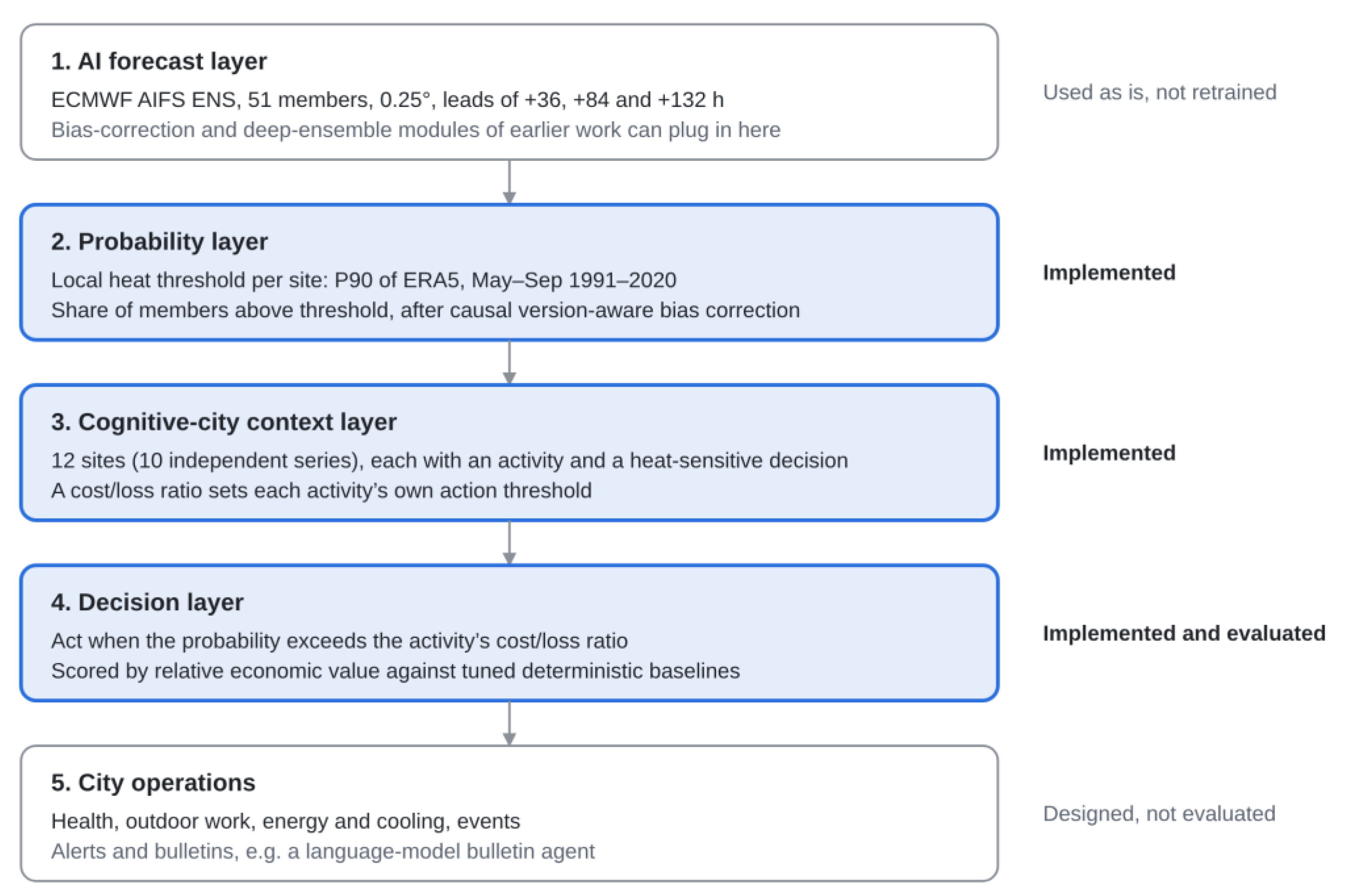
Figure 2.
Methodology: from 51 ensemble members to a scored decision for each city activity. Blue steps form the proposed layer; grey boxes show data, reference and comparison.
Figure 2.
Methodology: from 51 ensemble members to a scored decision for each city activity. Blue steps form the proposed layer; grey boxes show data, reference and comparison.
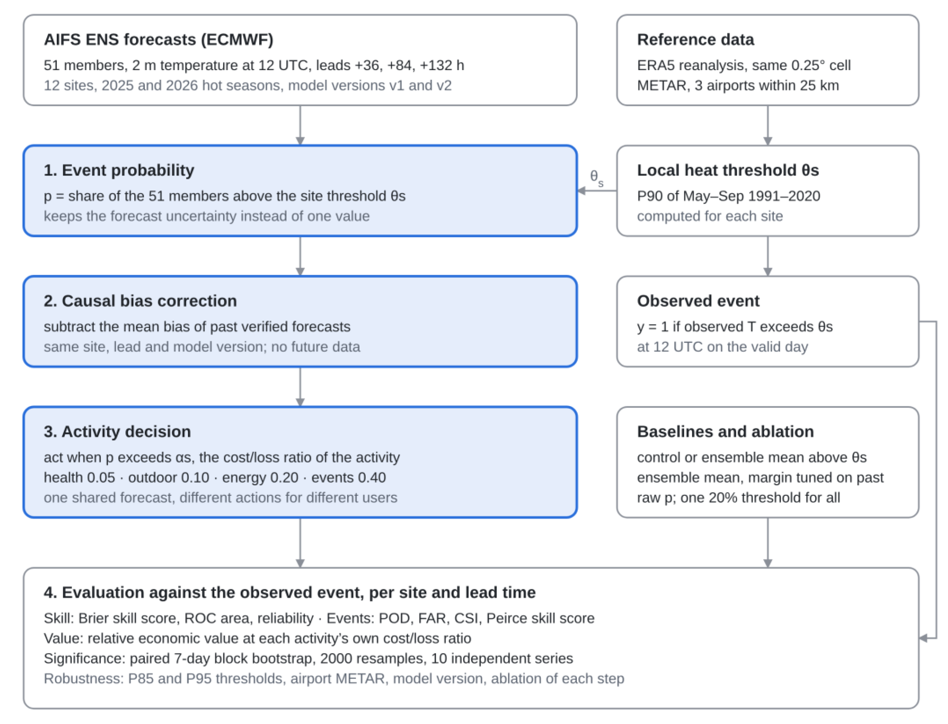
Figure 3.
(a) Relative economic value as a function of the cost/loss ratio, mean of ten series at +84 h; the tuned margin is re-fitted causally at each α, and vertical lines mark the four activity archetypes. (b) Reliability of raw and bias-corrected probabilities, all series and lead times; the inset enlarges probabilities below 0.2. Panel (a) averages all ten series at each α, whereas Table 7 averages only the series of each archetype at its own α, so the two need not agree for a given archetype.
Figure 3.
(a) Relative economic value as a function of the cost/loss ratio, mean of ten series at +84 h; the tuned margin is re-fitted causally at each α, and vertical lines mark the four activity archetypes. (b) Reliability of raw and bias-corrected probabilities, all series and lead times; the inset enlarges probabilities below 0.2. Panel (a) averages all ten series at each α, whereas Table 7 averages only the series of each archetype at its own α, so the two need not agree for a given archetype.
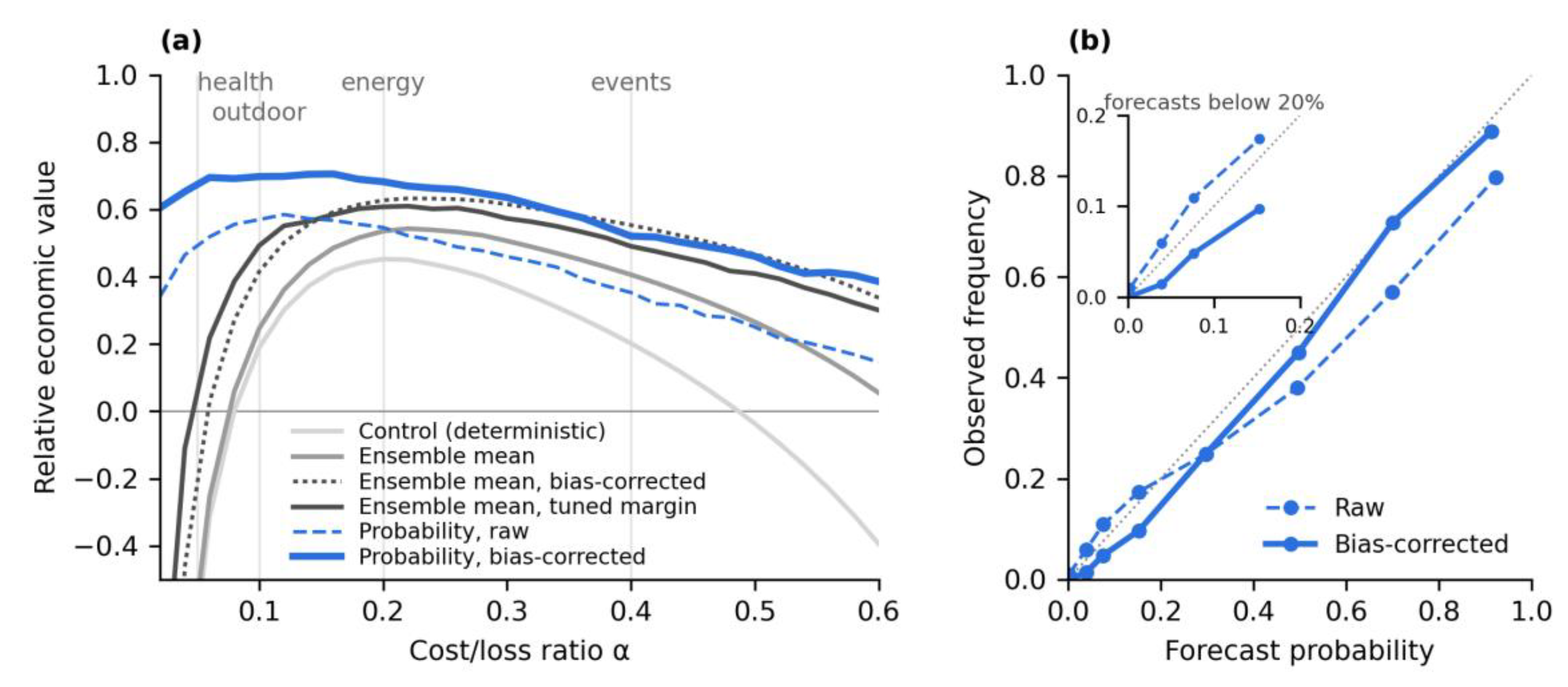
Figure 4.
One warning helps some activities and harms others; the probability serves all four. Relative economic value of the same KACST (Riyadh) forecasts at +84 h for four activities: one yes/no ensemble-mean warning (grey), the same warning after bias correction (dark diamond), the ensemble mean with a margin tuned causally for each activity (open circle), and the shared bias-corrected probability (blue). 244 forecasts, 66 events.
Figure 4.
One warning helps some activities and harms others; the probability serves all four. Relative economic value of the same KACST (Riyadh) forecasts at +84 h for four activities: one yes/no ensemble-mean warning (grey), the same warning after bias correction (dark diamond), the ensemble mean with a margin tuned causally for each activity (open circle), and the shared bias-corrected probability (blue). 244 forecasts, 66 events.
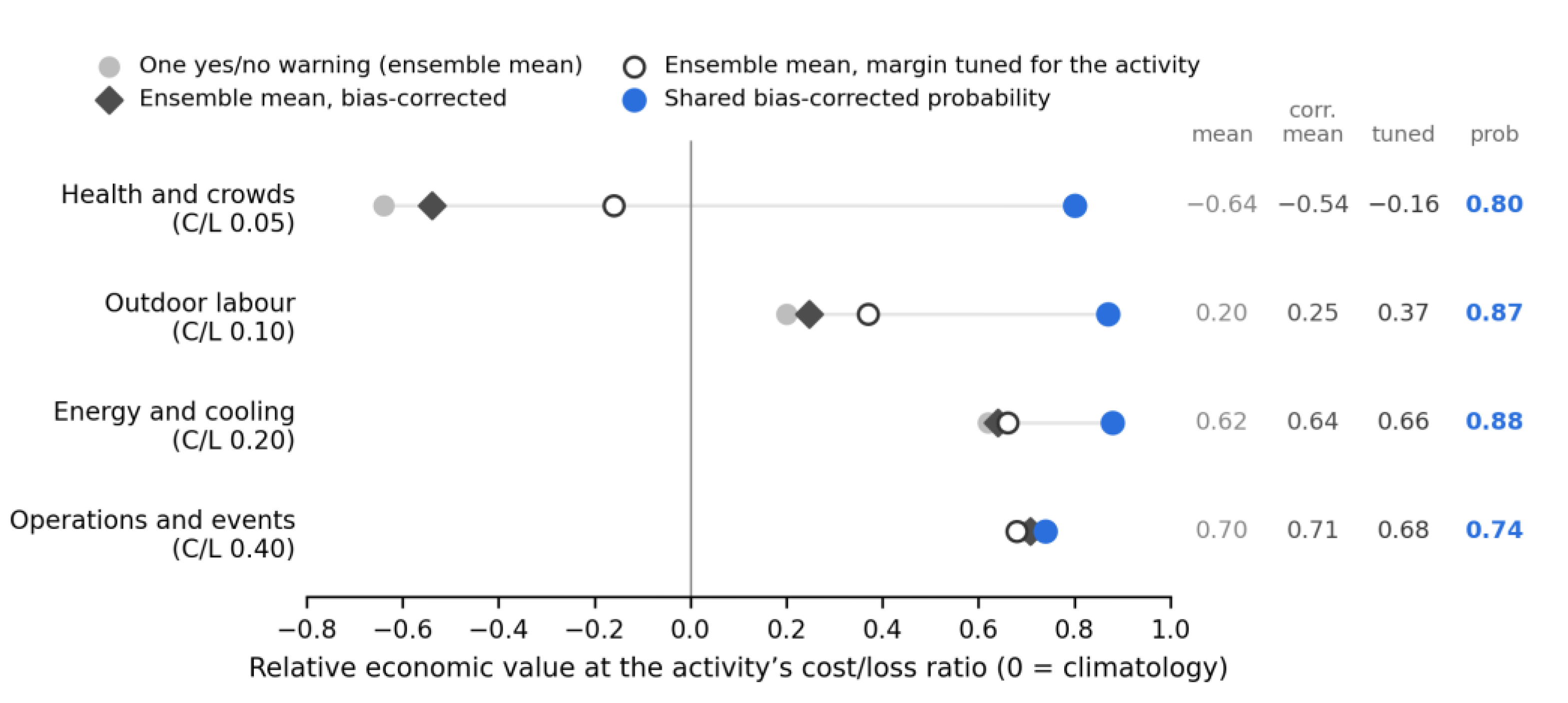
Table 1.
Positioning of this study against the closest related work.
| Study | Forecast | Decision users | Region | Value measured |
| Richardson [23] | Physics ensemble (ECMWF EPS) | Generic, any C/L | Northern extratropics | REV |
| Olivetti et al. [14] | IFS HRES vs. deterministic AIFS | One user per city, varying C/L | Exposed cities worldwide | Extended REV with penalties |
| Aitken et al. [26] | Blended AI–statistical, probabilistic | Heterogeneous farmers | India | Decision-theoretic, skill |
| Korhonen and Gregow [32] | ECMWF extended-range ensemble | Alert levels | Europe | Alert logic, no value |
| Alshehri [15] | GraphCast/WeatherNext 2 + deep ensemble | 12 sites, LLM bulletins | Saudi Arabia | Error, spread–error, rubric |
| This study | AIFS ENS probabilities | 4 activity types, 12 sites | Hyper-arid Saudi Arabia | REV per activity vs. tuned baselines, stations |
REV, relative economic value; C/L, cost/loss ratio.
Table 2.
Cognitive-city sites, heat-sensitive decisions and decision archetypes.
| Site | Status | Heat-sensitive decision | Archetype | C/L |
| KEC (Madinah) | Existing | Shade, cooling and water for visitors and religious events | Health and crowds | 0.05 |
| Jazan Industries | Future | Stop or shift exposed industrial work | Outdoor labour | 0.10 |
| DTV (Dhahran) | Existing | Schedule field work at energy sites | Outdoor labour | 0.10 |
| KAEC (Rabigh) | Existing | Shift outdoor loading and logistics work | Outdoor labour | 0.10 |
| SPARK (Eastern) | Future | Protect equipment and schedule yard work | Outdoor labour | 0.10 |
| KACST (Riyadh) * | Existing | Prepare backup cooling for laboratories and data centres | Energy and cooling | 0.20 |
| KAUST (Thuwal) | Existing | Schedule cooling load with renewable supply | Energy and cooling | 0.20 |
| KAPSARC (Riyadh) * | Existing | Prepare for peak electricity demand | Energy and cooling | 0.20 |
| NEOM – THE LINE | Future | Automated pre-cooling of buildings and mobility | Energy and cooling | 0.20 |
| NEOM – OXAGON | Future | Change port and manufacturing shifts | Operations and events | 0.40 |
| Misk City (Riyadh) † | Future | Postpone or move outdoor events | Operations and events | 0.40 |
| New Murabba (Riyadh) † | Future | Reschedule entertainment events | Operations and events | 0.40 |
* and † mark pairs that share a grid cell and an archetype; each pair is counted once in all statistics.
Table 3.
Decision rules compared.
| Rule | Decision input | Role |
| Climatology | Event base rate only | Reference for skill and value |
| Control forecast | Unperturbed member above θs | Deterministic baseline |
| Ensemble mean | Mean of 51 members above θs | Common-practice baseline |
| Ensemble mean, tuned margin | Mean above θs + m, m tuned causally per activity | Strong deterministic baseline |
| Ensemble mean, bias-corrected | Causally bias-corrected mean above θs | Baseline with the same bias correction |
| Probability, raw | Member fraction above αs | Ablation: no bias correction |
| Probability, one 20% threshold | Bias-corrected fraction above 0.20 | Ablation: no activity thresholds |
| Probability, bias-corrected | Bias-corrected fraction above αs | Proposed layer |
Table 4.
Local heat thresholds, number of events and ensemble-mean error against ERA5 at +84 h, by AIFS ENS version.
Table 4.
Local heat thresholds, number of events and ensemble-mean error against ERA5 at +84 h, by AIFS ENS version.
| Series | P90 (°C) | Events (of 244) | Bias (°C) | Bias v1 (°C) | Bias v2 (°C) | RMSE (°C) |
| KACST/KAPSARC (Riyadh) | 44.2 | 66 | −0.04 | −0.14 | +0.03 | 0.60 |
| Misk City/New Murabba | 43.6 | 68 | −0.35 | −0.43 | −0.29 | 0.71 |
| SPARK (Eastern) | 46.0 | 41 | +0.26 | +0.41 | +0.14 | 0.98 |
| DTV (Dhahran) | 38.7 | 50 | +0.24 | +0.41 | +0.12 | 0.76 |
| KEC (Madinah) | 43.8 | 37 | +0.74 | +0.44 | +0.97 | 1.02 |
| KAEC (Rabigh) | 41.7 | 37 | −0.81 | −0.19 | −1.26 | 1.34 |
| KAUST (Thuwal) | 37.1 | 52 | −1.85 | −1.51 | −2.09 | 1.99 |
| Jazan Industries | 34.2 | 27 | −0.05 | −0.25 | +0.10 | 0.62 |
| NEOM – THE LINE | 39.5 | 14 | +1.41 | +1.42 | +1.40 | 1.57 |
| NEOM – OXAGON | 34.1 | 23 | +0.27 | +0.24 | +0.29 | 0.61 |
v1: initialisations to 12 May 2026; v2: from 13 May 2026.
Table 5.
Brier skill score (BSS) and ROC area, mean of ten series.
| Forecast | BSS +36 h | BSS +84 h | BSS +132 h | ROC +36 h | ROC +84 h | ROC +132 h |
| Ensemble mean (continuous) | – | – | – | 0.96 | 0.95 | 0.94 |
| Probability, raw | 0.38 | 0.34 | 0.31 | 0.96 | 0.95 | 0.94 |
| Probability, bias-corrected | 0.59 | 0.52 | 0.45 | 0.96 | 0.95 | 0.93 |
BSS is not defined for the continuous ensemble mean.
Table 6.
Relative economic value at each series’ own cost/loss ratio, +84 h, and paired differences of the bias-corrected probability from the ensemble-mean warning, the bias-corrected ensemble-mean warning and the tuned rule.
Table 6.
Relative economic value at each series’ own cost/loss ratio, +84 h, and paired differences of the bias-corrected probability from the ensemble-mean warning, the bias-corrected ensemble-mean warning and the tuned rule.
| Series (archetype) | Ens. mean | Ens. mean, bias-corr. | Tuned margin | Prob., bias-corr. |
Prob. − mean [95% CI] |
Prob. − bias-corr. mean [95% CI] |
Prob. − tuned [95% CI] |
| KEC (health) | 0.72 | 0.41 | 0.56 | 0.70 | −0.02 [−0.14, 0.19] |
+0.30 [−0.11, 0.86] |
+0.15 [−0.05, 0.46] |
| Jazan (labour) | 0.24 | 0.18 | 0.19 | 0.52 | +0.28 [−0.11, 0.71] |
+0.34* [−0.02, 0.78] |
+0.33* [0.12, 0.67] |
| DTV (labour) | 0.53 | 0.42 | 0.63 | 0.66 | +0.13 [−0.07, 0.36] |
+0.24* [−0.03, 0.57] |
+0.03 [−0.14, 0.21] |
| KAEC (labour) | 0.28 | 0.58 | 0.63 | 0.68 | +0.39* [0.15, 0.67] |
+0.09 [−0.12, 0.30] |
+0.05 [−0.14, 0.26] |
| SPARK (labour) | 0.65 | 0.36 | 0.70 | 0.68 | +0.03 [−0.12, 0.22] |
+0.32* [0.08, 0.63] |
−0.02 [−0.10, 0.07] |
| KACST/KAPSARC (energy) | 0.62 | 0.64 | 0.66 | 0.88 | +0.25* [0.10, 0.48] |
+0.24* [0.08, 0.47] |
+0.22* [0.10, 0.40] |
| KAUST (energy) | −0.04 | 0.57 | 0.40 | 0.69 | +0.73* [0.54, 1.25] |
+0.12 [−0.06, 0.35] |
+0.29* [0.06, 0.65] |
| THE LINE (energy) | 0.68 | 0.80 | 0.75 | 0.61 | −0.07 [−0.50, 0.12] |
−0.20 [−0.94, −0.07] |
−0.14 [−0.75, 0.03] |
| OXAGON (events) | 0.62 | 0.68 | 0.71 | 0.62 | 0.00 [0.00, 0.00] |
−0.06 [−0.23, 0.12] |
−0.09 [−0.26, 0.00] |
| Misk/New Murabba (events) | 0.53 | 0.60 | 0.65 | 0.67 | +0.15* [0.03, 0.29] |
+0.07* [0.02, 0.14] |
+0.02 [−0.11, 0.16] |
Paired 7-day block bootstrap, 2000 resamples; * one-sided p < 0.05; intervals are two-sided, so a starred difference can have an interval that includes zero. At OXAGON the probability and the ensemble-mean warning issued identical warnings.
Table 7.
Mean relative economic value by activity archetype, +84 h.
| Archetype (C/L, series) | Control | Ens. mean | Ens. mean, bias-corr. | Tuned margin | Prob., raw | Prob., bias-corr. |
| Health and crowds (0.05, 1) | 0.52 | 0.72 | 0.41 | 0.56 | 0.53 | 0.70 |
| Outdoor labour (0.10, 4) | 0.32 | 0.43 | 0.39 | 0.54 | 0.65 | 0.63 |
| Energy and cooling (0.20, 3) | 0.38 | 0.42 | 0.67 | 0.60 | 0.45 | 0.73 |
| Operations and events (0.40, 2) | 0.41 | 0.57 | 0.64 | 0.68 | 0.54 | 0.65 |
Highest value in each row in bold.
Table 8.
Paired difference in relative economic value, bias-corrected probability with activity thresholds minus each alternative (mean of ten series, 95% block-bootstrap interval, one-sided p).
Table 8.
Paired difference in relative economic value, bias-corrected probability with activity thresholds minus each alternative (mean of ten series, 95% block-bootstrap interval, one-sided p).
| Alternative | +36 h | +84 h | +132 h |
| Ensemble mean | +0.20 [0.13, 0.31] p < 0.001 |
+0.19 [0.10, 0.30] p = 0.003 |
+0.22 [0.12, 0.36] p < 0.001 |
| Control forecast | +0.27 [0.18, 0.40] p < 0.001 |
+0.29 [0.20, 0.45] p < 0.001 |
+0.34 [0.22, 0.56] p < 0.001 |
| Ensemble mean, tuned margin | +0.09 [−0.01, 0.16] p = 0.033 |
+0.08 [−0.01, 0.18] p = 0.034 |
+0.10 [−0.01, 0.22] p = 0.035 |
| Ensemble mean, bias-corrected | +0.13 [0.03, 0.22] p = 0.02 |
+0.15 [0.03, 0.25] p = 0.01 |
+0.24 [0.09, 0.38] p = 0.002 |
| Raw probability | +0.12 [0.09, 0.24] p < 0.001 |
+0.11 [0.07, 0.25] p < 0.001 |
+0.11 [0.06, 0.24] p = 0.002 |
| One 20% threshold | +0.02 [−0.02, 0.09] p = 0.18 |
+0.03 [−0.02, 0.10] p = 0.10 |
+0.01 [−0.02, 0.06] p = 0.24 |
| Leave-one-month-out correction | −0.02 [−0.10, 0.02] |
−0.02 [−0.11, 0.03] |
−0.02 [−0.09, 0.02] |
| Probability, 5-day reference delay | +0.01 [0.00, 0.02] p = 0.10 |
+0.01 [−0.01, 0.03] p = 0.14 |
+0.01 [−0.01, 0.04] p = 0.18 |
Intervals are asymmetric because resamples with few events make relative economic value unstable. The last row compares the probability with the same probability when the bias correction may use only forecasts verified at least five days earlier. Doubling the one-sided values gives two-sided values of 0.07 at each lead time for the tuned margin and of 0.03, 0.03 and 0.003 for the bias-corrected ensemble mean. After a Holm correction of the two-sided values over the 18 comparisons in the first six rows, the differences from the ensemble mean, the control forecast and the raw probability at every lead time, and from the bias-corrected ensemble mean at +132 h, remain significant at the 0.05 level; the others do not.
Table 9.
Event verification at +84 h, counts pooled over ten series (415 events).
| Rule | POD | FAR | CSI | Peirce | Alarms per series |
| Control | 0.64 | 0.45 | 0.42 | 0.54 | 49 |
| Ensemble mean | 0.65 | 0.32 | 0.50 | 0.59 | 40 |
| Ensemble mean, tuned margin | 0.80 | 0.45 | 0.49 | 0.67 | 60 |
| Ensemble mean, bias-corrected | 0.72 | 0.24 | 0.59 | 0.68 | 39 |
| Probability, raw | 0.83 | 0.55 | 0.41 | 0.62 | 77 |
| Probability, bias-corrected | 0.92 | 0.51 | 0.47 | 0.72 | 79 |
| Probability, one 20% threshold | 0.93 | 0.44 | 0.53 | 0.78 | 70 |
244 forecasts per series.
Table 10.
Verification against airport METAR observations at +84 h, station-based 1991–2020 P90 threshold.
Table 10.
Verification against airport METAR observations at +84 h, station-based 1991–2020 P90 threshold.
|
Station (site, km) |
Events | Bias (°C) | BSS |
ROC prob./mean |
Value prob. | Value mean | Value tuned |
Prob. − mean [95% CI], p |
| OEMA (KEC, 12) |
16 | −0.04 | 0.35 | 0.97/0.97 | 0.75 | 0.78 | 0.76 | [−0.51, 0.25] p = 0.63 |
| OERK (KACST, 24) |
56 | −0.11 | 0.57 | 0.96/0.96 | 0.80 | 0.70 | 0.74 | [−0.02, 0.27] p = 0.07 |
| OEDR (DTV, 4) |
40 | −4.13 | 0.26 | 0.88/0.89 | 0.50 | −0.79 | 0.14 | [0.65, 2.12] p < 0.001 |
About 241 forecasts per station; bias of the uncorrected ensemble mean against the station.
Table 11.
Bias-corrected ensemble mean and tuned rule at the airport stations, +84 h: value of the bias-corrected ensemble-mean warning and paired differences of the bias-corrected probability from it and from the tuned rule.
Table 11.
Bias-corrected ensemble mean and tuned rule at the airport stations, +84 h: value of the bias-corrected ensemble-mean warning and paired differences of the bias-corrected probability from it and from the tuned rule.
| Station (site, km) | Value, bias-corr. mean | Prob. − bias-corr. mean [95% CI], p | Prob. − tuned [95% CI], p |
| OEMA (KEC, 12) | 0.78 | −0.04 [−0.53, 0.24] p = 0.64 |
−0.02 [−0.47, 0.26] p = 0.59 |
| OERK (KACST, 24) | 0.79 | +0.01 [−0.09, 0.12] p = 0.43 |
+0.06 [−0.02, 0.19] p = 0.09 |
| OEDR (DTV, 4) | −0.10 | +0.60 [0.16, 1.19] p = 0.001 |
+0.35 [−0.14, 1.07] p = 0.10 |
Each station uses its own causal bias correction; tuned margin range −6 to +2 °C (Section 3.5).
Table 12.
Verification at the grid cell of each of ten airports against METAR observations, +84 h: station-based 1991–2020 P90 threshold, Brier skill score of the bias-corrected probability and relative economic value of the bias-corrected probability, the ensemble-mean warning, the bias-corrected ensemble-mean warning and the tuned rule, averaged over the four activity cost/loss ratios (0.05, 0.10, 0.20 and 0.40).
Table 12.
Verification at the grid cell of each of ten airports against METAR observations, +84 h: station-based 1991–2020 P90 threshold, Brier skill score of the bias-corrected probability and relative economic value of the bias-corrected probability, the ensemble-mean warning, the bias-corrected ensemble-mean warning and the tuned rule, averaged over the four activity cost/loss ratios (0.05, 0.10, 0.20 and 0.40).
| Station (airport) | Grid cell (°N, °E) | Events | Bias (°C) | BSS | Prob. | Ens. mean | Bias-corr. mean | Tuned |
| OEAH (Al-Ahsa) | 25.25, 49.50 | 49 | −1.36 | 0.52 | 0.61 | −0.69 | 0.26 | 0.31 |
| OEDF (Dammam) | 26.50, 49.75 | 50 | −0.52 | 0.60 | 0.62 | 0.22 | 0.33 | 0.49 |
| OEDR (Dhahran) | 26.25, 50.25 | 40 | −4.13 | 0.26 | 0.41 | −0.89 | −0.20 | 0.00 |
| OEGN (Jazan) | 17.00, 42.50 | 12 | −2.84 | −0.12 | −0.02 | 0.00 | −0.07 | −0.17 |
| OEJN (Jeddah) | 21.75, 39.00 | 42 | −3.29 | 0.25 | 0.08 | −0.98 | −0.26 | −0.34 |
| OEMA (Madinah) | 24.50, 39.75 | 16 | −0.52 | 0.40 | 0.54 | 0.37 | 0.64 | 0.63 |
| OERK (Riyadh) | 25.00, 46.75 | 56 | −0.21 | 0.56 | 0.72 | 0.42 | 0.67 | 0.55 |
| OETB (Tabuk) | 28.50, 36.50 | 15 | +0.42 | 0.49 | 0.64 | 0.69 | 0.64 | 0.67 |
| OEWJ (Al Wajh) | 26.25, 36.50 | 14 | +2.08 | −1.68 | −0.29 | −1.37 | −0.01 | −0.17 |
| OEYN (Yanbu) | 24.25, 38.00 | 25 | −0.78 | 0.32 | 0.45 | −0.10 | 0.07 | 0.34 |
| Mean of ten airports | 0.16 | 0.37 | −0.23 | 0.21 | 0.23 |
About 241 forecasts per station; bias of the uncorrected ensemble mean against the station. Each station uses its own causal bias correction and a tuned margin range of −6 to +2 °C. The Dammam threshold is based on 15 years of reports within 1991–2020. Differences are tested with a 7-day block bootstrap using the same blocks at all airports.
Disclaimer/Publisher’s Note: The statements, opinions and data contained in all publications are solely those of the individual author(s) and contributor(s) and not of MDPI and/or the editor(s). MDPI and/or the editor(s) disclaim responsibility for any injury to people or property resulting from any ideas, methods, instructions or products referred to in the content. |
© 2026 by the authors. Licensee MDPI, Basel, Switzerland. This article is an open access article distributed under the terms and conditions of the Creative Commons Attribution (CC BY) license (http://creativecommons.org/licenses/by/4.0/).
Copyright: This open access article is published under a Creative Commons CC BY 4.0 license, which permit the free download, distribution, and reuse, provided that the author and preprint are cited in any reuse.