

Submitted:
16 November 2026
Posted:
18 November 2026
Read the latest preprint version here
Abstract
Purpose. Studies of Medicare claims rest on many small processing decisions about who enters the cohort, how drug exposure is defined and how follow-up is handled. These choices are rarely varied or reported together, so a single published estimate may reflect them as much as the underlying association. Methods. We used the 2008–2009 CMS DE-SynPUF Sample 1 synthetic Medicare claims file (116,352 beneficiaries; 114,538 alive at baseline). The outcome was hospitalization during 2009 and the exposure was any prescription drug claim in 2008. We crossed four cohort rules, two exposure definitions, two follow-up rules and two adjustment sets into 32 specifications and estimated the risk difference in each with robust standard errors. We tested the whole set jointly with the specification-curve procedure of Simonsohn and colleagues (500 resamples under a forced null) and measured how much of the variation each decision explains. Results. Risk differences ranged from 0.46 to 8.26 percentage points (median 3.89). Twenty-five of 32 specifications were significant, all in the positive direction, and the joint tests rejected the null (all P < 0.01). The cohort rule explained 66.1% of the variation among the estimates and the follow-up rule 15.4%; the exposure definition (0.05%) and covariate adjustment (0.01%) explained almost none. Requiring full-year Part D coverage raised the share classed as exposed from 62.3% to 97.5%. Conclusions. In this synthetic cohort the direction of the association was stable, but its size depended mainly on cohort eligibility rules rather than on the exposure definition or adjustment. Claims studies should report eligibility sensitivity analyses alongside their primary estimate. The data are synthetic and all findings are associational; no causal or drug-safety inference is intended.
Keywords:
specification curve
; claims data
; Medicare
; DE-SynPUF
; analytic flexibility
; pharmacoepidemiology
Key Points
- The estimated association between any 2008 drug claim and 2009 hospitalization was positive in all 32 defensible specifications of a synthetic Medicare cohort, but its size ranged from 0.46 to 8.26 percentage points.
- Cohort eligibility and follow-up rules explained more than 80% of the spread; the exposure definition and adjustment for age, sex and race explained almost none.
- Claims studies should show how their main eligibility rules change the estimate, not only vary the model.
1. Introduction
Estimates from administrative claims depend on decisions made long before a model is fitted [1]. Analysts choose how many months of enrollment a person needs, whether managed-care enrollees are kept, whether drug-benefit coverage is required, how exposure is read from prescription records, and how follow-up is defined. Jensen and colleagues showed that differences in enrollment and benefit-use requirements alone changed estimates of disease prevalence in a large commercial claims database [2]. Such choices are usually fixed once, described briefly, and not varied, so readers cannot tell how much of a reported association belongs to the data and how much to the processing.
Specification-curve analysis offers a way to show this. It lists every defensible, non-redundant analysis, displays the estimate from each in rank order alongside the decisions that define it, and tests the whole set with a joint inference procedure [3]. It extends the earlier idea of a multiverse analysis, in which a raw data set is processed in every reasonable way and the results are compared [4]. The approach has been applied to nutritional epidemiology, where 1,208 analytic specifications for red meat and all-cause mortality in NHANES produced estimates on both sides of no effect [5], and related work has shown that the choice of adjustment variables alone can reverse the direction of observational associations [6]. The approach has not, to our knowledge, been applied to the raw cohort-building decisions of a Medicare claims study, where the set of specifications is defined by eligibility rules rather than by modelling choices.
The CMS Data Entrepreneurs’ Synthetic Public Use File (DE-SynPUF) is a freely available synthetic file with the structure of the 5% Medicare sample [7]. CMS states that it was built for software development and training and that inferences about the Medicare population should not be drawn from it. It is therefore a safe and open setting for demonstrating methods, and has been used to illustrate a clone-censor-weighting design in a myocardial infarction cohort [8]. Because anyone can download it, an analysis on it can be reproduced exactly.
Our objective was methodological. Using a single DE-SynPUF sample, we asked how much the estimated association between any prescription drug claim in 2008 and hospitalization in 2009 changes across 32 defensible combinations of cohort, exposure, follow-up and adjustment decisions; whether the set of estimates as a whole is distinguishable from no association; and which of the decisions drives the spread. The data are synthetic, so we make no claim about drugs or about Medicare beneficiaries. The contribution is the framework and the open code.
2. Methods
2.1. Data Source and Study Design
We analysed DE-SynPUF Sample 1, a synthetic file that follows the structure of the 5% Medicare beneficiary sample [7]. The unit of analysis was the beneficiary. Baseline was calendar year 2008, in which we measured Part A, Part B and managed-care (HMO) months, Part D coverage and prescription drug events (PDE). Follow-up was calendar year 2009. One analysis file was built from the beneficiary summary, PDE and inpatient claims files, with one row per beneficiary (116,352 rows, 38 columns). Raw files were imported into PostgreSQL and cleaned: the cleaned prescription file held 5,552,421 events and the cleaned inpatient file 66,705 Segment 1 claims for 37,780 beneficiaries. All 116,352 beneficiaries were kept through left joins, so a beneficiary with no observed claim was classified as unexposed and not hospitalized; absence of a claim does not prove absence of a drug or a hospitalization. Of the 116,352 beneficiaries, 114,538 were alive at the start of follow-up and form the analysis population. The study is reported in line with the RECORD statement for studies using routinely collected health data [9].
2.2. Outcome and Exposure
The outcome was hospitalization in 2009, a binary indicator for at least one Segment 1 inpatient claim in 2009; the 68 Segment 2 claim lines in the file were not used. The exposure was any prescription drug use in 2008, defined from PDE records. The primary definition (strict NDC) required at least one 2008 PDE record with a valid 11-digit numeric national drug code (NDC), a positive quantity dispensed and a positive days supply; the alternative definition kept the NDC and days-supply requirements but dropped the quantity requirement. Two further definitions that relaxed the NDC requirement classified exactly the same beneficiaries as the strict definition and were not carried forward as separate specifications.
2.3. Step 1: The Specification Set
Following Simonsohn and colleagues [3], we listed the defensible decisions that define an analysis and crossed them in full (Table 1), giving 4 × 2 × 2 × 2 = 32 specifications. The four cohort rules differ in who counts as eligible. Every rule required survival to 1 January 2009. The ‘no Part D’ rule required 12 months of Part A and of Part B in 2008 and no HMO months. The primary rule added 12 months of Part D coverage. The other two relaxed one condition of the primary rule: HMO months were allowed, or no Part B condition was imposed (12 months of Part A, no HMO months and full-year Part D were still required). The two follow-up rules either kept everyone alive at the start of 2009 or kept only those with fee-for-service coverage throughout 2009, defined as 12 months of Part A and no HMO months in 2009 (Part B months were not part of this definition). Adjusted models added age, sex and race.
2.4. Estimation
In each specification we regressed the hospitalization indicator on the exposure by ordinary least squares. The exposure coefficient is the risk difference, which we report in percentage points with 95% confidence intervals from heteroskedasticity-robust (HC0) standard errors and a normal approximation. A specification was called significant at a two-sided 5% level. All specifications were estimated on the same 114,538 beneficiaries, restricted by each specification’s own rules.
2.5. Step 2: DISPLAY
2.6. Step 3: Joint inference
We tested three summaries of the whole curve: the absolute median risk difference, the number of specifications significant in the dominant direction, and a Stouffer combined Z, |Σz|/√32. To obtain their distribution under no association, we forced the null in every specification by subtracting the fitted effect from the outcome (the outcome minus the estimated risk difference times the exposure), so that the exposure had no estimated relation to it in that specification. We then resampled beneficiaries with replacement, using the same resampled rows in all 32 specifications to preserve their dependence, re-estimated all 32 and recomputed the three summaries. This was repeated 500 times with a fixed seed in a Python implementation; the SAS implementation reproduced the observed estimates and test statistics exactly and agreed with the Python resampling results in a 50-resample run. A P value was the share of resamples at least as extreme as the observed value, reported as < 1/500 when none were [3].
2.7. What Drives the Spread
We summarised the mean risk difference at each level of each decision, the paired change when one decision was switched and the others held fixed, and the share of the variance among the 32 estimates explained by each decision (sequential sums of squares from a four-factor model, with the remainder attributed to interactions).
2.8. Descriptive Denominators
Following Jensen and colleagues [2], we also tabulated the size of the cohort and the prevalence of exposure, hospitalization and full-year fee-for-service coverage as each rule was added cumulatively and as each was applied alone, and tested whether people with each outcome more often met the stricter rules (chi-square).
2.9. Supplementary Weighted Analysis
In the primary cohort we estimated a propensity score for exposure from age, sex and race by logistic regression, formed inverse-probability weights, compared standardised mean differences before and after weighting [10], and estimated a weighted risk difference.
2.10. Software and Reproducibility
The analysis file was prepared in PostgreSQL by a sequence of table-building steps (Appendix S3). Each rebuilt step was checked against the existing table, row by row and in both directions, with no differences (116,352 beneficiaries in the enrollment and prescription tables and 36,636 in the primary-cohort inpatient table), and the hospitalization rule reproduced the original claim counts exactly in the primary cohort (9,146 Segment 1 claims; 0 mismatches). Descriptive tables and the 32 estimates were produced in SAS OnDemand for Academics (PROC REG with robust standard errors), with built-in integrity checks that stop the program if any expected count or estimate differs. The 500-resample joint test and the null curves were produced in an independent Python implementation that reproduced every SAS estimate. An AI assistant (Claude, Anthropic) helped write and check the analysis code; the author ran all code and verified the output against the source data and against the independent SAS and Python implementations. The SAS, Python and SQL code, with the seeds, are provided as Supporting Information.
2.11. Ethics STATEMENT
This was a secondary analysis of a public synthetic file that contains no real beneficiaries, so no ethics review was required. The study is descriptive and methodological, and every estimate is an association.
3. Results
3.1. Cohort rules Change Who Is Analysed
Each eligibility rule reshaped the population (Table 2). Applying all primary rules left 36,636 of 116,352 beneficiaries (31.5%). Over the same steps the share classed as exposed rose from 62.3% to 97.5%, almost entirely at the final step that required full-year Part D coverage, and the share hospitalized in 2009 rose from 16.2% to 18.1%.
The rules were related to both exposure and outcome. Among exposed beneficiaries 81.6% had full-year Part D coverage, against 6.2% of the unexposed, and 49.3% met all primary rules, against 2.1% (both P < 0.0001). Hospitalized beneficiaries also more often met all primary rules than those not hospitalized (35.2% vs 30.8%, P < 0.0001), although the no-HMO rule alone did not differ by hospitalization (77.1% vs 76.9%, P = 0.45).
3.2. The Specification Curve
The 32 risk differences ranged from 0.46 to 8.26 percentage points, with a median of 3.89 (Figure 1; Table S1). All were positive. Twenty-five were significant at the 5% level; the seven that were not comprised six of the eight specifications that dropped the Part D requirement and one in the primary cohort (the unadjusted, full-fee-for-service, no-quantity-requirement specification, P = 0.053).
The curve rises in steps that line up with the cohort rule. The cohorts without a Part D requirement gave 0.46 to 0.62 points. The primary cohort gave 2.74 to 4.97, the cohort allowing HMO months 5.12 to 5.56, and the cohort with no Part B condition 2.73 to 8.26. Within a cohort, the exposure definition and adjustment changed the estimate by about 0.2 points or less, while restricting to full-year fee-for-service coverage lowered it, most strongly in the cohort with no Part B condition (from about 8.2 to 2.7 points).
3.3. Joint Tests of the Whole Curve
The set of 32 estimates as a whole was inconsistent with no association on all three summaries (Table 3). No resample under the forced null produced a median risk difference or combined Z as large as observed; two of 500 produced as many significant specifications. The observed curve lay above the 97.5th percentile of the null curves at 31 of the 32 ranks (Figure 2).
3.4. What Drives the Spread
The cohort rule explained 66.1% of the variation among the 32 estimates and the follow-up rule 15.4% (Table 4; Figure 3). The exposure definition (0.05%) and covariate adjustment (0.01%) explained almost none, and interactions between decisions accounted for the remaining 18.4%. Averaged over the other decisions, the mean risk difference was 0.54 points for the no-Part-D cohort, 3.88 for the primary cohort, 5.34 when HMO months were allowed and 5.55 with no Part B condition.
When one decision was switched and the rest held fixed, moving from the primary cohort to the no-Part-D cohort lowered the estimate by 3.34 points on average (range 2.28 to 4.38), allowing HMO months raised it by 1.47 and dropping the Part B requirement raised it by 1.67. Full-fee-for-service follow-up lowered it by 1.93 on average (range 0.07 to 5.47), the quantity requirement by 0.11, and adjustment changed it by 0.04.
3.5. Weighted Analysis in the Primary Cohort
In the primary cohort, where 97.5% were exposed, the crude risk difference was 4.92 points and the inverse-probability-weighted estimate 4.51 (Table 5). Before weighting, the standardised mean differences between exposed and unexposed were 0.17 for female sex, 0.08 for age and 0.13 for one race category; after weighting all were below 0.02.
4. Discussion
In this synthetic Medicare cohort the sign of the association between 2008 drug use and 2009 hospitalization was the same in all 32 defensible specifications, and the whole set was inconsistent with no association. Its size was not stable: it ranged from 0.46 to 8.26 percentage points, and two decisions about who is in the cohort and how long they are followed explained over 80% of that spread. How exposure was read from the prescription records and whether age, sex and race were adjusted for explained almost none of it.
The dominance of the cohort rule has a plain explanation in the data. Requiring full-year Part D coverage changed who was observed as well as how many: the share classed as exposed rose from 62% to 98%, and the people who remained had very different coverage histories (Table 2). A comparison between a large exposed group and a small, unusual unexposed group is not the same comparison as one between two sizeable groups, and it is not surprising that the estimate moved with it. The association in the primary cohort is therefore best read as one between benefit use and hospitalization among people enrolled throughout the year, not as a property of the drug exposure itself. This fits the earlier finding that enrollment and benefit-use requirements alter prevalence estimates in claims [2].
Specification-curve and vibration-of-effects studies elsewhere have mostly varied models and covariates, and found that the choice of adjustment set alone can move or reverse an association [5,6]. We found the opposite pattern for covariates: adjustment for age, sex and race changed estimates by less than 0.1 point. The fragility here came from the cohort rules, which are rarely written as analytic choices at all because they are usually treated as a design step. Claims analyses can therefore be sensitive to decisions that sit outside the model, and the usual sensitivity analysis over covariates would not have shown it.
Three practical points follow. First, studies using claims should report the effect of the main eligibility rules on the estimate, for example by showing the estimate under each rule alone and under their combination, in the manner of a cohort attrition table [2]. This is in keeping with reporting guidance that asks authors to describe how the study population was selected and how data were cleaned [9]. Second, a short specification curve over the few rules that are genuinely debatable is cheap and shows readers how much of a result belongs to the rule. Third, joint inference across the curve answers a different question from any single estimate: it asks whether the set of results, as chosen, could have arisen from no association [3]. Here it could not, but that says nothing about whether the association is causal or what its size is.
Our example sits alongside recent tutorial work that uses DE-SynPUF for a different purpose, a target-trial-style comparison of treatment initiation windows [8]. That work studies one cohort of patients with myocardial infarction and estimates a causal contrast under clone-censor-weighting. Ours asks a different question: how much an association in the whole beneficiary file depends on cohort, exposure, follow-up and adjustment decisions, quantified across 32 specifications with joint inference. The two are complementary.
4.1. Limitations
Several limitations apply. The data are synthetic and CMS advises against inference about the Medicare population [7], so the size of the associations here has no substantive meaning; only the behaviour of the method does. We used one DE-SynPUF sample, and the pattern may differ in other samples or in real claims. The exposure was any prescription drug claim and the outcome any hospitalization, so the exposure is not a specific drug and the comparison mixes people who differ in health and in benefit use. Only age, sex and race were available for adjustment, and unmeasured confounding is likely to be large in claims data generally [11]; the estimates are associations and not effects. In the primary cohort 97.5% of beneficiaries were exposed, so fewer than 1,000 were unexposed, which limits precision and raises a positivity concern for the weighted analysis. The specification set reflects our judgement of which decisions are defensible, is not exhaustive, and other analysts might list a different set. The joint tests rely on forcing the null by subtracting a fitted linear effect and on resampling beneficiaries as independent rows; with 500 resamples the smallest reportable P value is 0.002. The outcome definition was not varied: Segment 2 claim lines were not counted and alternative inpatient claim-date rules were not examined, and deaths during 2009 were retained although they shorten follow-up. Finally, we used a linear probability model for a binary outcome, and our search of the literature was not exhaustive, so the statement that the approach is new for Medicare cohort rules should be read as ‘to our knowledge’.
5. Conclusion
In a synthetic Medicare cohort, the direction of the association between any prescription drug claim and later hospitalization was stable across 32 defensible specifications, but its size depended mainly on who was eligible and how follow-up was defined, and hardly at all on the exposure definition or on adjustment for age, sex and race. Claims studies should report how their main eligibility rules change the estimate, and a specification curve is a practical way to do so.
5.1. Plain Language Summary
Researchers who use insurance claims make many small choices about which people to include and how to define who took a drug. We tested 32 reasonable combinations of these choices in a public, computer-made (synthetic) Medicare file. The link between taking any prescription drug in 2008 and being in hospital in 2009 always pointed in the same direction, but its size changed more than sixteen-fold. Most of that change came from the rules for who was included, not from how drug use was defined or from adjusting for age, sex and race. Because the data are synthetic, the results say nothing about real patients or drugs; they show why studies using claims should report how their inclusion rules affect their results.
Ethics Statement
This study used a publicly available, fully synthetic data set and involved no human participants, so institutional review was not required.
Supplementary Materials
The following supporting information can be downloaded at the website of this paper posted on Preprints.org. Additional supporting information can be found online in the Supporting Information section: Table S1 (all 32 specifications with estimates; included at the end of this file); Appendix S1 (SAS program); Appendix S2 (Python verification code); Appendix S3 (SQL used to build the analysis file).
Author Contributions
O.D.O. conceived the study, prepared the data, performed the analyses and wrote the manuscript.
Funding
The author received no specific funding for this work.
Data Availability Statement
The DE-SynPUF files are publicly available from CMS [7]. The SAS program (including the resampling seed), the Python verification code and the SQL used to build the analysis file are provided as Supporting Information and are archived with a permanent identifier at Zenodo (https://doi.org/10.5281/zenodo.24269311).
Acknowledgments
AI disclosure: Claude (Anthropic) was used as an assistant for code development and checking and for editing the manuscript. The author designed the study, ran and verified all analyses, and is responsible for the content.
Conflicts of Interest
The author declares no conflicts of interest.
Prior Presentations
None.
References
- Schneeweiss, S.; Avorn, J. A review of uses of health care utilization databases for epidemiologic research on therapeutics. J. Clin. Epidemiol. 2005, 58(4), 323–337. [Google Scholar] [CrossRef]
- Jensen, E.T.; Cook, S.F.; Allen, J.K.; et al. Enrollment factors and bias of disease prevalence estimates in administrative claims data. Ann. Epidemiol. 2015, 25(7), 519–525.e2. [Google Scholar] [CrossRef]
- Simonsohn, U.; Simmons, J.P.; Nelson, L.D. Specification curve analysis. Nat. Hum. Behav. 2020, 4(11), 1208–1214. [Google Scholar] [CrossRef]
- Steegen, S.; Tuerlinckx, F.; Gelman, A.; Vanpaemel, W. Increasing transparency through a multiverse analysis. Perspect. Psychol. Sci. 2016, 11(5), 702–712. [Google Scholar] [CrossRef]
- Wang, Y.; Pitre, T.; Wallach, J.D.; et al. Grilling the data: application of specification curve analysis to red meat and all-cause mortality. J. Clin. Epidemiol. 2024, 168, 111278. [Google Scholar] [CrossRef]
- Patel, C.J.; Burford, B.; Ioannidis, J.P.A. Assessment of vibration of effects due to model specification can demonstrate the instability of observational associations. J. Clin. Epidemiol. 2015, 68(9), 1046–1058. [Google Scholar] [CrossRef]
- Centers for Medicare; Medicaid Services. CMS 2008-2010 Data Entrepreneurs’ Synthetic Public Use File (DE-SynPUF). Medicare Claims Synthetic Public Use Files. CMS: Baltimore, MD. Available online: https://www.cms.gov (accessed on 15 November 2026).
- Webster-Clark, M.; Li, Y.; Dell’Aniello, S.; Platt, R.W. Demystifying clone-censor-weighting to studying treatment initiation windows: an example using publicly available synthetic Medicare claims data. Pharmacoepidemiol Drug Saf. 2025, 34, e70223. [Google Scholar] [CrossRef]
- Benchimol, E.I.; Smeeth, L.; Guttmann, A.; et al. The REporting of studies Conducted using Observational Routinely-collected health Data (RECORD) statement. PLoS Med. 2015, 12(10), e1001885. [Google Scholar] [CrossRef]
- Austin, P.C. Balance diagnostics for comparing the distribution of baseline covariates between treatment groups in propensity-score matched samples. Stat. Med. 2009, 28(25), 3083–3107. [Google Scholar] [CrossRef]
- Brookhart, M.A.; Stürmer, T.; Glynn, R.J.; Rassen, J.; Schneeweiss, S. Confounding control in healthcare database research: challenges and potential approaches. Med. Care 2010, 48((6) Suppl, S114–S120. [Google Scholar] [PubMed]
Figure 1.
Specification curve. The 32 risk differences (percentage points) in rank order with 95% confidence intervals (upper panel), with significant estimates in blue and non-significant estimates as grey open circles, above a panel marking the option of each decision (cohort rule, exposure definition, follow-up rule, adjustment) that defines each specification. All 32 estimates are positive.
Figure 1.
Specification curve. The 32 risk differences (percentage points) in rank order with 95% confidence intervals (upper panel), with significant estimates in blue and non-significant estimates as grey open circles, above a panel marking the option of each decision (cohort rule, exposure definition, follow-up rule, adjustment) that defines each specification. All 32 estimates are positive.
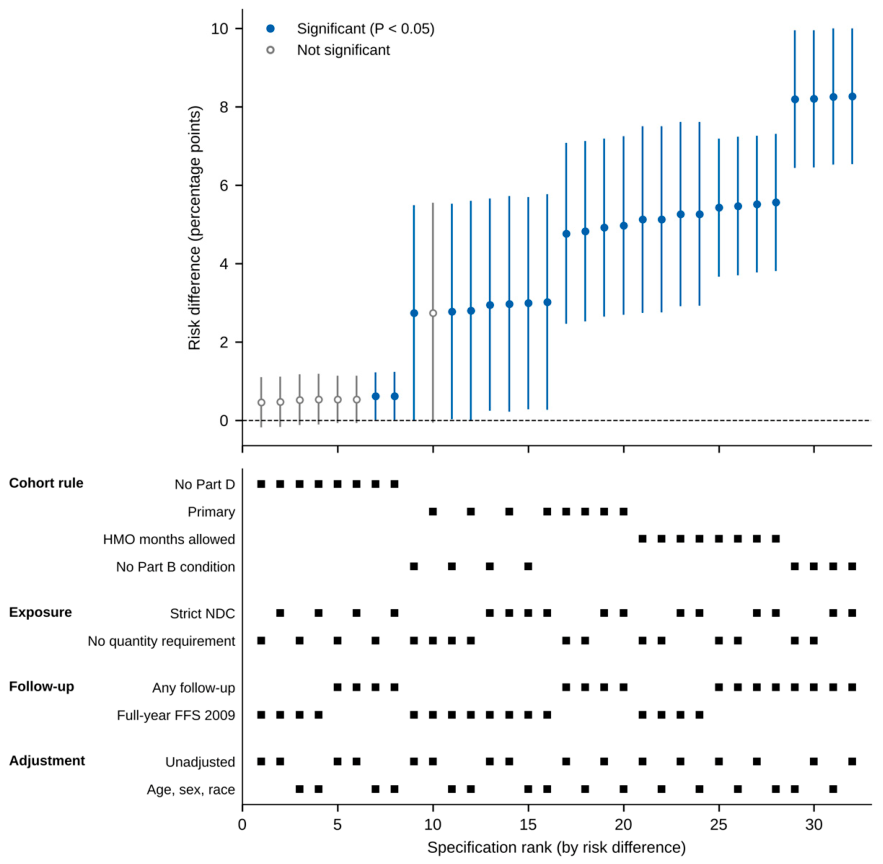
Figure 2.
Observed specification curve against the null. The observed ranked risk differences are compared with the 2.5th, 50th and 97.5th percentile bands of the ranked estimates across 500 resamples with the null forced in every specification. The observed curve lies above the 97.5th percentile at 31 of 32 ranks.
Figure 2.
Observed specification curve against the null. The observed ranked risk differences are compared with the 2.5th, 50th and 97.5th percentile bands of the ranked estimates across 500 resamples with the null forced in every specification. The observed curve lies above the 97.5th percentile at 31 of 32 ranks.
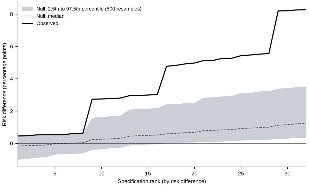
Figure 3.
Share of variation among the 32 estimates explained by each analytic decision: cohort rule 66.14%, follow-up rule 15.37%, exposure definition 0.05%, adjustment 0.01%, interactions 18.43%.
Figure 3.
Share of variation among the 32 estimates explained by each analytic decision: cohort rule 66.14%, follow-up rule 15.37%, exposure definition 0.05%, adjustment 0.01%, interactions 18.43%.
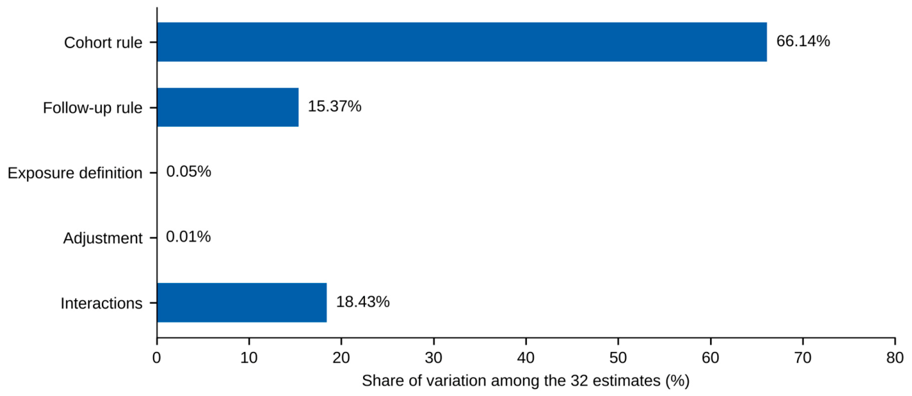

Table 1.
The 32 specifications are the full cross of these four decisions.
| Decision | Options | Number |
| Cohort rule | No Part D requirement; primary (full-year Part D); HMO months allowed; no Part B condition | 4 |
| Exposure definition | Strict NDC with positive quantity and days supply; same without the quantity requirement | 2 |
| Follow-up rule | Any follow-up; fee-for-service coverage throughout 2009 (12 months Part A, no HMO) | 2 |
| Adjustment | Unadjusted; adjusted for age, sex and race | 2 |
HMO, health maintenance organization; NDC, national drug code. Total specifications = 4 × 2 × 2 × 2 = 32.
Table 2.
Cohort size and outcome prevalence as eligibility rules are added cumulatively.
| Population | N | % of all | % exposed (2008) | % hospitalized (2009) | % full-year FFS (2009) |
| All beneficiaries | 116,352 | 100.0 | 62.3 | 16.2 | 65.5 |
| + alive at start of 2009 | 114,538 | 98.4 | 62.6 | 16.4 | 65.5 |
| + ≥ 6 months Part A and B in 2008 | 100,285 | 86.2 | 68.9 | 17.9 | 69.4 |
| + 12 months Part A and B in 2008 | 95,605 | 82.2 | 69.7 | 18.2 | 69.2 |
| + no HMO months in 2008 | 72,071 | 61.9 | 62.4 | 18.4 | 90.0 |
| + full-year Part D in 2008 (primary cohort) | 36,636 | 31.5 | 97.5 | 18.1 | 93.2 |
FFS, fee-for-service (12 months of Part A and no HMO months in 2009); HMO, health maintenance organization. % full-year FFS is calculated among the 114,538 beneficiaries with a 2009 enrollment record; the 1,814 who died before 2009 have none.
Table 3.
Joint tests of the specification curve (null forced in every specification; 500 resamples).
Table 3.
Joint tests of the specification curve (null forced in every specification; 500 resamples).
| Test | Observed | Resamples as or more extreme | P |
| Median risk difference | 3.89 points | 0 of 500 | < 0.002 |
| Specifications significant (P < 0.05) | 25 of 32 | 2 of 500 | 0.004 |
| Stouffer combined Z | 22.46 | 0 of 500 | < 0.002 |
Observed values from SAS and Python (identical). P values are the share of 500 resamples at least as extreme as observed; the smallest reportable P is 0.002.
Table 4.
Contribution of each analytic decision to the spread of the 32 risk differences.
| Decision | Change examined (others held fixed) | Mean paired change, points (range) | Variance explained, % |
| Cohort rule | Primary → no Part D requirement | −3.34 (−4.38 to −2.28) | 66.14 |
| Primary → HMO months allowed | +1.47 | ||
| Primary → no Part B condition | +1.67 | ||
| Follow-up rule | Add full-year FFS restriction | −1.93 (−5.47 to −0.07) | 15.37 |
| Exposure definition | Add quantity requirement | −0.11 | 0.05 |
| Adjustment | Add age, sex and race | +0.04 | 0.01 |
| Interactions | — | — | 18.43 |
Mean risk difference by cohort rule (points): no Part D requirement 0.54; primary 3.88; HMO months allowed 5.34; no Part B condition 5.55. FFS, fee-for-service; HMO, health maintenance organization.
Table 5.
Supplementary weighted analysis in the primary cohort (N = 36,636).
| Measure | Before weighting | After weighting |
| Risk difference, points | 4.92 (crude) | 4.51 (IPW) |
| Standardised mean difference, female sex | 0.17 | < 0.02 |
| Standardised mean difference, age | 0.08 | < 0.02 |
| Standardised mean difference, race category | 0.13 | < 0.02 |
IPW, inverse-probability weighted. The propensity score used age, sex and race.
Disclaimer/Publisher’s Note: The statements, opinions and data contained in all publications are solely those of the individual author(s) and contributor(s) and not of MDPI and/or the editor(s). MDPI and/or the editor(s) disclaim responsibility for any injury to people or property resulting from any ideas, methods, instructions or products referred to in the content. |
© 2026 by the author. Licensee MDPI, Basel, Switzerland. This article is an open access article distributed under the terms and conditions of the Creative Commons Attribution (CC BY) license.
Copyright: This open access article is published under a Creative Commons CC BY 4.0 license, which permit the free download, distribution, and reuse, provided that the author and preprint are cited in any reuse.