
Submitted:
16 November 2026
Posted:
18 November 2026
You are already at the latest version
Abstract
Detectors emit a bounded number of boxes per image, usually one constant: COCO sweeps maxDets = [1, 10, 100], LVIS fixes max_dets = 300. Images differ in count, so a fixed bound is slack on sparse and binding on dense ones. Given a fixed total of boxes, does redistributing them between images help? We show that it is a distributional rather than an overall performance intervention. Our allocation is proportional to each image's annotated object count, so it is an oracle diagnostic, not a deployable policy. On validation it raises worst-image recall by 5.3 to 10.9 points over three seeds and both heads, but the micro-averaged recall difference is approximately 1.5 points (+1.30 to +1.49 across the six seed-by-head runs), equivalence within the prespecified ±1.0-point margin is not established, and mean recall falls 6.2 to 6.8 points. It changes which image is worst rather than lifting every image: after reallocation the uniform-quota worst image is replaced by a different one. The cost is graded: the sparsest 5% lose 24 points and every band changes sign. Once the budget exceeds the label-count cap everywhere the two allocations coincide and the comparison is vacuous.
Keywords:
object detection
; output budget
; budget reallocation
; worst-case recall
; detection evaluation protocol
; VisDrone
1. Introduction
A detector’s output budget is the largest number of boxes it may emit for an image. It is rarely treated as a scientific choice. The COCO evaluation protocol sweeps maxDets = [1, 10, 100] [1]; the LVIS protocol fixes max_dets = 300 [2]; the reference implementations in common use default to 300. In each case a single constant is applied to every image in the benchmark, whatever those images contain.
That constant is not innocuous, and the observation is not new. Dave et al. [3] raised the detections-per-image limit on LVIS from 300 to 10,000 and reported that mean average precision rises from 22.6 to 26.1, with the average precision for rare categories rising from 12.6 to 19.8. The same intervention leaves COCO essentially unchanged at 37.4 to 37.5, which they attribute to COCO’s smaller vocabulary. The first-place entry in the 2021 LVIS challenge reports a consistent effect on a different metric, with boundary AP rising from 44.1 to 45.3 as the per-image limit increases from 300 to 1,000, and notes that the competition rules imposed no limit at all [4]. Oksuz et al. [5] report from a third direction that localisation recall precision responds to detections-per-image, although in their setting average precision and oLRP move in opposite directions, so the two metrics do not agree on the sign of the change. Ultralytics issue #25992 [6] records an aggregate ceiling of the same kind: at the default limit, the fraction of annotated objects recoverable by construction is 23.6% on the benchmark discussed there.
Those reports are consistent with a fixed output budget being able to bind. All of them act by raising the limit, which gives every image more boxes. None asks what follows when the limit is genuinely fixed, which is the situation in any deployed system with a hard quota. A concrete case is a downlink that can carry a fixed number of boxes per frame for a whole camera array, so that boxes spent on one camera are boxes denied to another. If the budget is fixed and the constraint binds, the distribution across images becomes a free parameter: the same total number of boxes can be spread evenly, concentrated on dense images, or allocated in any other way. Whether that freedom is worth exercising is an open question. The evaluation literature treats the output budget as a protocol constant rather than an allocatable resource, and the allocation literature that would supply the machinery addresses other budgets: compute or patch selection rather than emitted boxes [7], or a decision-theoretic value of perception compute under a budget-constrained oracle with uniform inference as the baseline [8]. Two lines do reallocate a per-sample capacity, but of computation rather than emitted boxes: content-aware detectors give each image a data-dependent compute budget [9], and computation reallocation moves backbone FLOPs across resolutions [10]. In retrieval and recommendation, a fixed output window has been formalised as a deterministic ceiling on achievable ranking quality [11,12], but there the window is per query or per user, leaving no room for redistribution.
We therefore ask a narrow question. Given a fixed total number of boxes to distribute across an image set, does reallocating it change the worst-image recall, and what does the change cost? We answer with a measurement rather than a method. The proportional allocation we compare against is a GT-proportional rule with a per-image cap, obtained by integer water-filling, and we claim nothing new for it [13,14]. What we contribute is the magnitude of the effect on a real detector, the distribution of its cost across the images, and the regime in which the comparison is vacuous.
We evaluate this on VisDrone2019-DET [15] with YOLO26n [16], whose two prediction heads give two settings within one detector, and we train three seeds. Reallocating a fixed total budget raises worst-image recall by 5.3 to 10.9 points on validation, but under the same label-informed diagnostic it does not change on the test-dev split. Three results constrain how that gain should be read.
First, the intervention is distributional rather than absolute, and we use the word operationally: the reallocation changes the identity and the distribution of image-level recall rather than producing a uniform improvement, so a higher minimum does not imply that every image, or the average image, improves. It changes which image attains the minimum; some images gain, others lose. When we trace the identity of the worst image under both allocations, the uniform allocation consistently pins a dense image as the worst case, and reallocation replaces it with a different one. Mean per-image recall therefore falls even as the minimum rises.
Second, the total box count is conserved and the cost is graded. Micro-averaged recall changes by approximately 1.5 percentage points, and for the six seed-by-head runs the change is +1.2978 to +1.4938 points; equivalence within the pre-specified ±1.0-point margin is not established (Methods). The reason the total is close to fixed is that when the budget binds on every image the number of boxes that can be spent is fixed by the budget. The cost falls unevenly: the sparsest 5% of images lose 24.2 points while the densest quartile gains 10.1, and mean per-image recall falls by 6.2 to 6.8 points. A practitioner who adopts per-image allocation to protect the worst case will redistribute recall towards images that already contained the most objects.
Third, the boundary of the effect is structural, not empirical. Once the budget exceeds the annotated count on every image, the label-count cap binds everywhere and the two allocations coincide exactly; we verify this by exact comparison of the two quota vectors. Any "zero gain" measured there is an identity, and we report it as such rather than as evidence about the allocation.
This work sits between three literatures that do not meet. Detection evaluation treats the per-image output limit as a protocol constant, and the reports that show it can bind act by raising it, which gives every image more boxes rather than moving boxes between images [3,4,5]. Resource-allocation work in detection budgets compute or input regions rather than emitted outputs, and has already argued that allocation should be judged against a budget-constrained oracle with uniform inference as a baseline [7,8]. Information retrieval and recommendation formalise a fixed output window as a hard ceiling on achievable ranking quality [11,12], but the window there is fixed per query or per user, so no redistribution is possible. What has been missing is a measurement of what redistribution actually buys, and at whose expense.
Two things follow for practice. First, worst-image recall is an extreme order statistic governed by whichever image happens to be worst, so treating it as a deployment objective moves the loss onto the images with the fewest objects rather than reducing it. Second, before per-image allocation is adopted, the budget should be checked against what the detector can actually emit: if the budget is not binding, the allocation question does not arise, and a comparison run there will return zero for structural reasons. We report these results for one detector on one benchmark, and we state the scope explicitly rather than generalising.
2. Results
2.1. R0. Output-Budget Utilisation Varies by Up to 8.5-Fold Across Detection Benchmarks
A detector’s output budget is the maximum number of boxes it may emit per image. In practice this budget is a fixed constant: the COCO evaluation protocol sweeps maxDets = [1, 10, 100] [1], the LVIS protocol fixes max_dets = 300 [2], and the Ultralytics YOLO implementation defaults to max_det = 300 [16]. Whether that is reasonable depends on , because a fixed budget binds only on images whose count exceeds it.
We therefore computed, for six benchmark splits, three quantities that depend only on the label distribution and not on any model: the mean per-image object count, the budget utilisation , and the fraction of images whose count exceeds the budget, . Supplementary Table S8 reports them and Figure 1 shows them as curves.
At , utilisation spans 0.074 to 0.630 and the fraction of images on which the budget binds spans 0.000 to 0.195. The ordering is not an artefact of that budget: it is unchanged at B = 50 and B = 200. The ordering follows the mean object count, not the domain. highD and VisDrone validation are both aerial, yet their mean counts differ by a factor of 2.7 and their utilisation by 2.4, so the split is by density rather than by whether the camera flies. The largest object count does not predict utilisation either. CrowdHuman contains images with 391 annotated people, more than any VisDrone validation image (317), yet only 2.1% of CrowdHuman images exceed a budget of 100, against 19.5% of VisDrone validation images.
Two cautions apply. CrowdHuman flags ignore regions per box; excluding them lowers the mean object count by 3.8% and from 0.021 to 0.018, leaving the ordering unchanged. Supplementary Table S8 bounds the room a reallocation has; whether recall changes depends on the detector, not the labels.
2.2. R1. Reallocation is Positional: Worst-Image Recall Rises While Mean Per-Image Recall Falls
To test whether the budget is better distributed than by a uniform constant, we trained YOLO26n on VisDrone2019-DET and evaluated on the 548-image validation split, for three seeds. For a fixed total budget with , we compared three allocations of the same total: a uniform quota with c chosen so that ; a quota proportional to the true object count (an oracle, see Methods), with a the largest multiplier whose spend stays within S; and an adaptive variant that caps each quota at alone rather than at . Here is the number of boxes the detector can emit for image i, which caps the quota. Quotas are integers. At = 0.5 the two arms spend 19,325 and 19,376 boxes of the nominal , a pairwise difference of 0.26% and a largest deviation from S of 0.28%.
On validation, proportional allocation raises worst-image recall by 5.31 to 10.87 points across the three seeds and both heads (Figure 2), and Figure 3 resolves the change image by image. Replacing the label count with the detector’s own prediction count as the allocation signal recovers part of this gain at about half the mean cost (Methods; Supplementary Table S2). The gain is positive in every resample on five of the six seed-by-head conditions and in 99.72% on the sixth, the one-to-one head at seed 42. It is not a general improvement: mean per-image recall falls by 6.21 to 6.77 points on the same comparisons, so the intervention raises the minimum by lowering the average. Micro-averaged recall changes by 1.30 to 1.49 percentage points across the six seed-by-head runs. When the budget binds on every image, the number of boxes that can be spent is fixed at by the budget rather than by the allocation. That identity constrains boxes emitted and not objects recovered: the false-positive share of the spent boxes rises with the budget, from under 1% at two boxes per image to over 40% at seventy, so the identity bounds the total recall instead of fixing it. Reallocating a fixed budget redistributes recall; total recall rises by only 1.30 to 1.49 points, for which equivalence within the pre-specified 1.0-point margin is not established.

Table 1.
Allocation of a fixed output budget at = 0.5, VisDrone2019-DET validation (N = 548). The arm is the no-top-up allocation; its values were reconstructed deterministically from the corrected per-image true-positive prefix records, as described in Methods and implemented in the Table 1 reconstruction package (Supplementary Information). Worst-image recall is ; mean per-image recall is the unweighted mean of over images. Cells are ordered one-to-many head (first entry) / one-to-one head (second entry); within each entry, seeds 42, 43 and 44 follow in that order. CI is estimated using a paired bootstrap over images; the analysis code sets the resampling RNG seed to 20261014. True positives are assigned with the corrected matcher of Section 4.3 (class-agnostic, IoU threshold 0.5, unmatched boxes only); = 0.5 and N = 548 images per seed. The current results registry specifies 10,000 resamples per seed. Differences are computed from unrounded values before rounding.
Table 1.
Allocation of a fixed output budget at = 0.5, VisDrone2019-DET validation (N = 548). The arm is the no-top-up allocation; its values were reconstructed deterministically from the corrected per-image true-positive prefix records, as described in Methods and implemented in the Table 1 reconstruction package (Supplementary Information). Worst-image recall is ; mean per-image recall is the unweighted mean of over images. Cells are ordered one-to-many head (first entry) / one-to-one head (second entry); within each entry, seeds 42, 43 and 44 follow in that order. CI is estimated using a paired bootstrap over images; the analysis code sets the resampling RNG seed to 20261014. True positives are assigned with the corrected matcher of Section 4.3 (class-agnostic, IoU threshold 0.5, unmatched boxes only); = 0.5 and N = 548 images per seed. The current results registry specifies 10,000 resamples per seed. Differences are computed from unrounded values before rounding.
| Quantity | Uniform | Proportional | Difference (pt) |
|---|---|---|---|
| Worst recall, o2m | 11.67 /11.99 /11.99% | 20.00 /20.37 /20.00% | +8.33 /+8.38 /+8.01 |
| Worst recall, o2o | 11.36 /11.67 /11.36% | 16.67 /20.00 /22.22% | +5.31 /+8.33 /+10.87 |
| Total recall (micro), o2m | 40.75 /40.82 /41.07% | 42.25 /42.17 /42.48% | +1.49 /+1.35 /+1.40 |
| Total recall (micro), o2o | 40.12 /40.28 /40.57% | 41.58 /41.58 /41.89% | +1.46 /+1.30 /+1.32 |
| Mean recall (macro), o2m | 50.41 /50.63 /50.96% | 43.99 /44.03 /44.19% | −6.42 /−6.60 /−6.77 |
| Mean recall (macro), o2o | 49.25 /49.51 /50.02% | 43.04 /43.27 /43.57% | −6.21 /−6.24 /−6.45 |
| 95% CI for gain, o2m | n/a | n/a | [+5.86,+13.01] /[+5.63,+13.01] /[+5.86,+13.33] |
| 95% CI for gain, o2o | n/a | n/a | [+1.93,+11.18] /[+5.26,+10.91] /[+7.48,+14.13] |
| , o2m | n/a | n/a | 1.0000 /1.0000 /1.0000 |
| , o2o | n/a | n/a | 0.9972 /1.0000 /1.0000 |
All budget-sweep values in this section, and in Figure 2, Figure 3 and Figure 4, were computed with the earlier matcher implementation described in Section 4.3; the corrected matcher was applied to the six runs at = 0.5 reported in Table 1, and the other budgets have not been recomputed under it. The one-to-many gain moves from +11.15 to +8.78 points and the one-to-one gain from +8.24 to +6.40 at , while at the one-to-one gain moves in the opposite direction, from +3.93 to +7.65. The direction of the effect is stable, but its magnitude is not resolvable at the precision a single seed would suggest, which is why we report ranges rather than point estimates throughout, and why the confidence intervals extend past the threshold we pre-specified.
2.3. R2. The Cost of the Reallocation Falls on the Sparsest Images
Because the total box count is conserved, only the distributional consequences matter. Table 2 breaks the per-image recall change down by object-count band, for the one-to-many head at = 0.5 (Figure 4).
The gain is concentrated in the densest quartile (+10.07 points) and the loss in the sparsest images (−24.20 points). The sparsest band holds 27 images, so its interval is widest, at 12.14 points, yet excludes zero: the cost is present in every one of the 10,000 resamples. Every band’s interval excludes zero, and the interval ordering matches the band ordering, so under this scheme the gradient is not an artefact of band membership. In VisDrone, sparse images are those containing few and comparatively large objects: mean box area is 2. of the frame in the sparsest 5% against 1. in the densest quartile, and the Spearman correlation between object count and mean box area is −0.46 (Figure 5). The shift is distributional: the 5th percentile rises 5.84 to 9.68 points while the median falls (Figure 6, Supplementary Table S7). We deliberately do not infer object distance from this, because the benchmark provides no depth annotation and the relation between size and distance in aerial imagery also depends on camera tilt. Optimising worst-image recall therefore raises the recall of the dense images, which start from the lower baseline, and lowers that of the sparse images, which start from the higher baseline. Maximising the minimum is not the same objective as improving the worst case in the sense that matters for deployment.
Table 2.
Per-image recall by object-count band, VisDrone2019-DET validation, one-to-many head, seed 42, = 0.5. is proportional minus uniform, in points. The band boundaries are fixed by the label distribution, which does not depend on the model. Bands are formed by sorting images on and cutting at fixed ranks, so images that share an object count can fall in adjacent bands; the cuts are rank quantiles rather than disjoint value intervals, the range column reports the observed span within each band, and no model output enters the cut. The interval is a paired percentile bootstrap over images within the band (10,000 resamples; the RNG is derived per seed so that re-running one seed alone reproduces its row), so it estimates the mean cost of the band and not the membership of the band. The one-to-one head gives the same ordering with slightly smaller magnitudes: and points at the two extremes, both intervals excluding zero. These band values come from the earlier matcher run and are descriptive; the corrected recomputation on the same images gives and points for the sparsest and densest bands, a difference of 0.01 points on the first. The bin-interpolation details of the original run are not recoverable, so the bands are reported as a description of the cost profile rather than as a re-derivation.
Table 2.
Per-image recall by object-count band, VisDrone2019-DET validation, one-to-many head, seed 42, = 0.5. is proportional minus uniform, in points. The band boundaries are fixed by the label distribution, which does not depend on the model. Bands are formed by sorting images on and cutting at fixed ranks, so images that share an object count can fall in adjacent bands; the cuts are rank quantiles rather than disjoint value intervals, the range column reports the observed span within each band, and no model output enters the cut. The interval is a paired percentile bootstrap over images within the band (10,000 resamples; the RNG is derived per seed so that re-running one seed alone reproduces its row), so it estimates the mean cost of the band and not the membership of the band. The one-to-one head gives the same ordering with slightly smaller magnitudes: and points at the two extremes, both intervals excluding zero. These band values come from the earlier matcher run and are descriptive; the corrected recomputation on the same images gives and points for the sparsest and densest bands, a difference of 0.01 points on the first. The bin-interpolation details of the original run are not recoverable, so the bands are reported as a description of the cost profile rather than as a re-derivation.
| band | Images | range | Uniform | Proportional | 95% interval for | |
|---|---|---|---|---|---|---|
| sparsest 5% | 27 | 1 to 9 | 76.85% | 52.64% | −24.20 | [−30.28,−18.14] |
| 5 to 25% | 110 | 10 to 39 | 67.92% | 46.11% | −21.81 | [−23.92,−19.69] |
| 25 to 50% | 137 | 40 to 65 | 56.70% | 44.26% | −12.44 | [−13.65,−11.28] |
| 50 to 75% | 137 | 65 to 93 | 44.44% | 43.64% | −0.80 | [−1.35,−0.26] |
| densest 25% | 137 | 93 to 317 | 30.03% | 40.10% | +10.07 | [+9.11,+11.07] |
2.4. R3. The Gain Depends on the Budget Fraction and Does Not Clear the Pre-Specified Threshold Uniformly
We specified a decision rule in the internal analysis plan: the allocation line would be treated as a standalone contribution if the worst-image gain reached 10 points, as a component of a larger study between 5 and 10 points, and abandoned below 5 points. The rule used the absolute point gain rather than a ratio, because a ratio would have required a denominator that a real detector cannot attain.
For seed 42, at the pre-specified budget fraction = 0.5 the point estimates are +8.33 points on the one-to-many head and +5.31 on the one-to-one head, both inside the middle band, and the 95% percentile intervals are [+5.86, +13.01] and [+1.93, +11.18] (Table 1). Both intervals extend past the 10-point threshold at their upper limits, and neither is bounded away from it, so the point estimate alone would understate the uncertainty. The measured effect is therefore too uncertain to decide whether the allocation is worth reporting as a standalone result, and we report it as a component while stating the uncertainty explicitly.
A no-top-up ablation is the only variant whose implementation and per-image records are preserved; at the eight conditions where both arms satisfy N1, it leaves the worst-image gain unchanged to four decimal places, while the micro-recall gain is 0.09 to 0.21 points higher than with the top-up (Supplementary Table S6). The gain is not an artefact of the budget fraction, but neither is it uniformly below the threshold; removing the label-count cap raises it further (Supplementary Table S5). Sweeping over {0.30, 0.40, 0.50, 0.60, 0.70} and both heads gives ten conditions spanning +4.25 to +10.21 points. The no-top-up configuration at = 0.30 spends 11,308 boxes against a target S = 11,627.7, while the proportional arm spends 11,620, so the no-top-up arm falls 2.75% short of S (312 boxes; the pairwise gap is 2.69% of the larger spend). That condition does not meet the 1% equal-spend rule (N1) and is reported descriptively only. Eight of the ten fall in the middle band; one condition reaches the standalone band: the one-to-many head at = 0.40 gives +10.21 points, which the pre-specified rule scores as A. The remaining condition, the one-to-one head at = 0.70, falls below 5 points and scores as C. The full sweep is reported in Supplementary Table S1 and plotted against in Supplementary Fig. S2; we do not report the pre-specified value alone, and we do not claim that the threshold is never reached.
2.5. R3b. The Effect is Hump-Shaped in the Budget
Supplementary Table S8 reports how much room a fixed budget leaves. That is a property of the labels; whether reallocating changes the worst-image recall is a property of the detector, and the two come apart. To separate them we swept the average per-image budget B from 2 to 500, holding the total spend identical across the two allocations at every budget (relative difference between spends below 10⌃-4). Panel a of Figure 2 plots the same gain against the budget. Actual emitted boxes match the target budget to within 0.006% in every spendable condition and pin at n at the two saturated ones (Supplementary Table S11). Of the 17 budgets, 12 are spendable: at neither allocation can spend the budget, because the label-count cap saturates every quota, and those budgets are excluded from the spendable sweep.
Three regimes appear, and we separate them by cause rather than by sign. At the smallest budgets the gain is negative on the one-to-many head, because proportional rounding gives an image with two to twenty objects one box where uniform gives two, so sparse images lose recall before dense ones gain. At intermediate budgets the gain peaks, at 11.15 points when , and the between-seed spread is largest there: the one-to-one head moves from +8.42 at B = 40 to +3.93 at B = 50, a range of 4.5 points across budgets and 4.8 points across seeds at fixed budget. At the gain is exactly zero, but for two different reasons: at the two quota vectors differ while the worst image is the same image at its cap under both, whereas at every budget from B = 100 to 500 (five values in all) the two vectors are equal entry by entry and the comparison is an identity. Across the sweep the total recall moves by at most 1.31 points, and across the budget fraction sweep by at most 1.40 points. The full sweep is reported in Supplementary Table S1.
2.6. R4. A Reproducible YOLO26n Baseline on VisDrone2019-DET
The detector used throughout is YOLO26n [16], trained from COCO weights [1] on the VisDrone2019-DET training split [15] for 100 epochs at 640×640 with batch size 8 on a single 8 GB consumer GPU. For seed 42, peak validation mAP50 is 0.3436 at epoch 83 and peak mAP50-95 is 0.1890 at epoch 82; the final-epoch values are 0.3385 and 0.1854. For seed 43 the two peaks coincide at epoch 80, at 0.3407 and 0.1858, with final-epoch values of 0.3365 and 0.1839. Seed 44 peaks at epoch 82, at 0.3421 and 0.1874, with final-epoch values of 0.3364 and 0.1838. The three seeds land within 0.3 points on mAP50 and 0.4 on mAP50-95, small relative to the between-seed spread of the allocation gain in R5b, and consistent with the effect being a property of how quotas interact with the label distribution rather than of detector quality. Training takes 238 s per epoch. We report no comparison against a published YOLO26n baseline: those figures used a different batch size and no stated seed. The per-epoch curve, the environment lock, and the weight hashes are released with the code, and the curves for all three seeds are plotted in Supplementary Fig. S1.
2.7. R5. The Gain is Positional, and Part of the Zero-Gain Regime is Structural
Supplementary Table S8 bounds the room a reallocation has. Whether it is worth using that room depends on the detector, and on which image the minimum lands on. Supplementary Table S9 reports the measured gain; Supplementary Table S10 reports the two quantities that decide it: whether the two quota vectors coincide, and the identity of the worst image under each allocation.
Three features of Supplementary Table S10 matter. At B = 100 and 300 the comparison is vacuous: the two quota vectors are equal entry by entry, which we verify by exact array comparison rather than by inspecting the gain, so both allocations collapse to the same quota vector under the label-count cap and the measured zero is an identity. At B = 70 the vectors differ on 314 of 548 images, yet the worst image is the same image under both allocations (index 22, with 12 annotated objects) and has reached its cap under both, so its recall is literally the same number and the minimum is taken over one unchanged value. Below B = 70 the gain is real and sign-varying: the largest is +11.15 points at B = 25, the smallest is −2.84 at B = 10, and the sign is not uniform across heads at B = 6 and 10.
The gain comes from the identity of the worst image changing. At B = 25 under a uniform quota the worst image is the densest one, with 317 annotated objects, held to 8.20% recall; redistribution moves quota to it, and the minimum is then taken over a different image at 19.36%. Some images gain and others lose (densest quartile +10.07 points, sparsest 5% -24.20); what changes is which image is worst. This is why the gain disappears once no image’s quota is binding, and why the intervention should not be described as an improvement of a fixed worst case.
2.8. R5b. What Replicates Across Seeds, and What Does Not
Two things replicate exactly and one does not. The allocation-side quantities are fixed by the quota vector, which depends on and the budget and not on the network weights: at = 0.5 the uniform worst-image recall is 11.67% for the one-to-many head on seed 42 and 11.99% on seed 43, and 11.36% and 11.67% respectively for the one-to-one head. The two heads are not interchangeable here. The same holds at , where quotas of one or two boxes quantise per-image recall to multiples of ; for the one-to-many head the gains are identical across seeds at B = 2 and B = 6, while for the one-to-one head they already differ, because the detector’s ordering no longer decides the minimum.
The zero-gain regime also replicates exactly, for the reasons given above: at B = 100 and 300 the two quota vectors are equal on all three seeds and both heads, and at B = 70 the worst image is the same one at its cap in all four combinations.
The magnitudes do not replicate, and we report them as ranges. The between-seed spread reaches 4.8 points on the one-to-one head, where the gain at B = 50 runs from +3.93 on seed 42 to +8.69 on seed 44, and at B = 25 both heads lose 2 to 3 points from the first seed to the second. Every magnitude in this paper is therefore a range over three seeds and two heads, and the ranges are wide enough that a single-seed comparison at a single budget could be made to show almost any effect within them.
3. Discussion
This work began as an attempt to predict, per image, whether an output budget should be reallocated. The prediction failed and we withdrew it. What survived is a measurement of what reallocation buys, what it costs, and when the question is vacuous. We report both halves, because the failure is informative about the shape of the problem.
The failed attempt is worth stating precisely, because the same construction is natural. We tried to decide, per image, whether the budget or the detector limited that image, by comparing the worst image’s quota against the number of boxes it could physically emit. The quantity is computable from stored predictions and needs no retraining. It is not diagnostic, for two reasons. First, shuffling the detector’s confidence-ordered hit sequences across images, which holds the label counts and the budget fixed while substituting another detector, leaves the verdict unchanged in 198 of 200 draws and makes the gain non-positive in each: the quantity tracks the labels, not the detector. Second, at seed 42 on the one-to-one head, ten non-degenerate conditions at budgets 58 to 67 predict a gain that is measured negative, down to −2.8 points; a counterexample, not a rate. The deeper reason is that a detector emits at least as many predictions as an image has annotated objects, so the prediction count cancels and the construction reduces to a statement about the labels alone, the same class of quantity as the utilisation statistics we already argued are uninformative. The only reliable test of such a quantity is to change the detector and see whether the verdict follows.
Under a uniform quota the densest image is pinned as the worst case; once the quota is redistributed it no longer is, so the minimum falls on a different image. The 5th percentile rises while the median falls: reallocation moves recall down the distribution rather than creating it. Describing this as an improvement of the worst case would be arithmetically accurate and substantively misleading, because the binding constraint moved rather than relaxed.
The zero-sum property follows from the same accounting, with one correction we owe the reader. When the budget binds on every image, the conservation identity fixes the spend. That identity is about boxes emitted, not about objects recovered: the false-positive share of the spent boxes rises with the budget, so the identity bounds the total recall rather than fixing it. Measured total recall changes by at most 1.41 points across the twelve spendable budget conditions, consistent with that bound; those budget-sweep values were computed with the earlier matcher, and at = 0.5 the corrected runs give to points. Reallocation is therefore not an overall performance improvement. It moves recall between images, and the images it moves recall away from are the sparsest ones, which in VisDrone contain the fewest and largest objects. Adopting worst-image recall as an objective therefore means, in this benchmark, degrading the easiest images to improve the hardest. That is a defensible choice for some applications and a poor one for others, but it should be made explicitly rather than inherited from a metric name.
The gain is bounded by the nature of the worst image. Because it replaces rather than improves that image, in the evaluated comparisons, the gain appeared on images for which additional detections yielded additional true positives. On validation the worst image is quota-limited, so the proportional allocation moves the minimum elsewhere. On test-dev both allocations share the same worst image: the uniform quota already covers its 8 boxes and recovers none (Supplementary Table S3), while the vectors differ on 1568 of 1610 images for the one-to-many head and 1569 for the one-to-one head, and both spend 37,551 boxes. The comparison is well posed and the gain is +0.000 on both heads. The mechanism replicates while the aggregate statistic does not.
Several limitations bound these claims. The results come from three training seeds of one detector on one benchmark; the between-seed spread is material, reaching 4.8 points on one head, so the magnitudes we report are ranges rather than points, including the 24.2-point loss on the sparsest images, whose interval spans 12.14 points and still excludes zero, and the 11.2-point peak gain. Above a per-image budget of about 100 the budget can no longer be spent in full, because the label-count cap saturates every quota; for those conditions the two allocations coincide exactly, and we report them as a structural identity rather than as evidence about allocation. CrowdHuman [17] object counts depend on an annotation convention, with ignored regions optionally excluded; we report both versions, and the cross-benchmark ordering is unchanged. Finally, the two heads we test are two settings of the same network rather than two independent implementations, so the measurement rests on one detector family.
Two directions follow. The measurement should be repeated on detectors whose per-image recall is flat in object count, since the positional gain is a property of the failure profile, not the allocation. The objective also deserves scrutiny: worst-image recall is an extreme order statistic whose sampling variability is governed by a handful of images, which is why the intervals we report are wide relative to the effect. Lower quantiles of the per-image recall distribution would trade the interpretability of a worst case for estimates a finite benchmark can actually resolve.
4. Methods
4.1. Detector and Training
We used YOLO26n as implemented in Ultralytics 8.4.177. YOLO26 is an end-to-end detector with two parallel heads over the same backbone: a one-to-many head that produces dense predictions and requires non-maximum suppression, and a one-to-one head that produces a fixed set of predictions and requires none. The one-to-one head is the head used at deployment; we report both, since the choice of head changes the allocation result by 3.0 points.
Training used the Ultralytics default optimiser with mosaic augmentation at 1.0, disabled for the final 10 epochs, translation 0.1, scale 0.5, horizontal flip 0.5, and HSV jitter (h 0.015, s 0.7, v 0.4). Mixup, copy-paste, and rotation were disabled to keep the recipe comparable to the published VisDrone anchor. Early stopping was disabled so that the full 100-epoch curve is available. Data-loader workers were set to 0, which is required on Windows: with workers > 0 the validation pass deadlocks during worker spawn.
4.2. Evaluation Protocol
Detection quality is reported as AP@[.50:.05:.95] following the VisDrone protocol. The validation split was used for all development; the test-dev split entered only the pre-specified decision rule, which is evaluated separately on both splits and takes the more conservative result. Both splits are processed through the same label-informed pipeline, so neither is an independent deployment test. Predictions were generated at confidence 0.001 with IoU 0.7, matching the COCO and LVIS sweeps.
For the budget experiments, the detector is run once with max_det set to the largest budget in the sweep. Smaller budgets are then obtained by truncating each image’s predictions to its top by confidence. This is exact rather than approximate: we verified on 40 images across eight budgets and both heads that truncating a large-max_det run reproduces running at the small max_det directly, with 40/40 images matching and a maximum coordinate deviation of 0.0. Because the equivalence holds, each budget costs no additional inference.
A full-resolution pass over all 548 validation images at once exhausts GPU memory, so the scan is run in chunks that are merged afterwards; the merge is checked against annotation counts recomputed from the label files, and any mismatch aborts the merge.
4.3. True-Positive Assignment and Matcher Version
True positives are assigned by a class-agnostic greedy matcher at an intersection-over-union threshold of 0.5. Predictions are processed in descending confidence, and ties in confidence are broken by the original prediction index, so the order is deterministic. At each step the prediction is compared against the ground-truth boxes that are still unmatched and is assigned to the one with the highest intersection over union; if that value is at least 0.5 the prediction counts as a true positive and the box becomes unavailable, otherwise the prediction counts as a false positive and no further ground-truth box is tried. This last clause is the substantive difference from the matcher used in our earlier runs, which selected the best-overlapping box among all annotations and then discarded the prediction if that box was already taken. The earlier behaviour under-counts true positives whenever the best-overlapping box for a prediction has been consumed by a higher-confidence prediction while a second, still-unmatched box would have met the threshold. The six validation comparisons reported in Table 1, one per seed-by-head combination at = 0.5, were computed with the corrected matcher, whose source file is src/eval/budget_scan.py (SHA-256 04C59D98…DF959E8). The test-dev figures in Section 4.11 were produced with the earlier implementation and are not comparable on this point.
4.4. Allocation
For a total budget , the uniform allocation gives every image the same quota c, chosen by bisection as the largest value for which . The proportional allocation is defined through the budget rather than directly: we bisect the multiplier a and give image i the quota for the largest a whose total spend does not exceed S. Writing the quota directly as would overspend, because the ceiling is applied per image; on the validation split at = 0.5 it exceeds S by 0.70% and changes 135 of 548 quotas. Quotas are rounded up to integers, and the spend of an allocation is . Every quota is capped at by construction: the term because the detector cannot emit more boxes than it predicts, and the term because this paper studies the label-count-capped regime, in which each image may be allocated at most as many boxes as it has annotated objects. That second cap is a modelling choice and not a property of the detector: because predictions are ranked by confidence, a box beyond the first can still be the first to match a previously unmatched object, so the cap removes output slots that could in principle raise recall. For every reported the global budget is fully spendable, and the worst image is not at the cap below B = 70; individual images whose annotated count falls below the uniform quota do reach the cap, and at the cap saturates the whole allocation; the saturation there is therefore label-count saturation, not exhaustion of the detector’s prediction capacity. Hence holds for every image at every budget we report, so this spend equals the number of boxes the detector actually emits, ; we checked the two sums agree exactly at every swept budget, on both heads, with a maximum difference of zero boxes, where is the number of predictions the detector emitted for image i. The three allocations are compared only when their spends agree to within 1%. Because is the annotated count, the proportional allocation is an oracle: it measures what redistribution could buy if each image’s object count were known in advance, not a deployable policy.
The proportional rule is the classical max-min fair rule for the total-spend constraint, and we use it as a baseline rather than as an optimum of the recall objective: which image ends up worst depends on where the detector’s errors fall, not only on how many boxes each image receives. That maximisation is a max-min fair allocation problem, and progressive water-filling is its standard solution [13]; we do not claim the optimisation as a new result. The per-image caps, the integer rounding and the top-up step mean the result is a capped proportional allocation rather than an exact max-min fair rule, and the quotas are set from object counts rather than from recall, so the allocation is not the solution that directly maximises the worst-image recall we evaluate. What we report is its behaviour when the constraint is the number of boxes a detector may emit, and the empirical consequences of that setting, which neither the optimisation literature nor the detection-evaluation literature addresses.
4.5. Prediction-Proportional Allocation
The proportional allocation above uses the annotated object count , which is not available at inference time; it therefore measures what redistribution could buy if each image’s object count were known in advance, and it is an oracle rather than a policy. To ask what the proportional rule would do if the allocation signal were the detector’s own output rather than the label count, we replace with the number of predictions the detector emits for that image once, at the largest budget in the sweep, . This signal is available at inference; the top-up below is not, so the resulting pipeline is label-informed throughout and is not a deployable policy. The same bisection, the same integer rounding, and the same top-up are applied, so the only change is the allocation signal.
On the one-to-many head the prediction-proportional variant recovers 53% to 78% of the oracle gain in worst-image recall (+5.72, +6.55 and +4.24 points for seeds 42, 43 and 44, against +8.33, +8.38 and +8.01 for the oracle), and it does so at roughly half the macro cost (−3.44, −3.49 and −3.83 points against −6.36, −6.57 and −6.87). On the one-to-one head it recovers almost none of the gain (+0.32 points), which is what the positional account predicts: on that head the worst image is already close to its ceiling under the uniform quota, so reallocation has little to replace. Because exceeds on every image in our records, the prediction-based signal is a noisy proxy for the oracle one, and the gap between the two rows is the price of not knowing the object count.
4.6. Spend Audit
Because two different sums are both called spend in this literature, we report both for every condition: the target total budget S, the nominal quota total , the number of boxes actually emitted , and the annotation-capped sum . Across the forty-two reported combinations, covering all three seeds, the two sums agree exactly, so no reported number depends on which one is used; the per-condition values are in Supplementary Table S11 and in results/tables/spend-audit.json. In the spendable conditions the emitted count matches the target to within 0.006%. At B = 100 and B = 300 the emitted count is pinned at = 38,759 rather than at = 299,100, which is the direct evidence that the saturation there comes from the label-count cap and not from the detector’s prediction capacity. No quota ever exceeds its annotated count, because the cap is imposed by construction, and on these records on all 548 images, so the term is always the binding one.
4.7. Budget Convention and Top-Up
Two conventions are easy to misread, so we state them explicitly. First, B is the total budget divided by the number of images, . It is an average per-image budget, not a cap on any single image: the uniform allocation fixes one quota c for every image, so an image whose capacity exceeds c can never receive more, but the proportional allocation can give an image several times B when that image is dense. At on the validation split the largest quota is 206 boxes under the uniform allocation and 312 under the proportional one, against an average of 70. Second, integer bisection alone usually underspends S by a few boxes. We therefore add a deterministic top-up: while the spend is below S, one box is added to the image whose next prediction carries the highest marginal true-positive gain. That gain is read off the label matches, so the top-up is label-informed; it is applied identically to every allocation, which keeps the comparison internally valid, but it means no allocation in this paper is a deployable policy. The top-up changes the quota of 0.4% of images at , 8.9% at and 1.1% at ; it is applied identically to every allocation, so it cannot favour one over another. Without it the two spends would differ and the comparison would confound where boxes go with how many are spent.
4.8. Top-Up Ablation
The main text reports the oracle top-up, which reads true-positive matches from the annotations. To test whether the reported gain depends on that choice, we repeated every condition without any top-up. The no-top-up arm is the only alternative whose implementation and per-image records are preserved; two further label-free top-up rules that we had explored are not reported here, because their implementations were not retained and their numerical records cannot be traced to code. Across = 0.40 to 0.70, both allocations satisfy the N1 spend condition under the no-top-up configuration (shortfall relative to S: 0.19 to 0.45% for the uniform allocation, 0.00 to 0.10% for the proportional one), and the oracle arm lies within 0.01% of S. At these eight conditions the worst-image gain is identical with and without the top-up (difference 0.0000 points in every case), whereas the micro-recall gain is 0.09 to 0.21 points lower with the top-up (1.38 versus 1.51 points at = 0.5 on the one-to-many head). At = 0.30 the no-top-up arm under-spends S by 2.75% and is therefore not a valid control there. Within the spend-matched conditions, the reported worst-image gain therefore does not depend on the true-positive information used by the top-up step. This comparison concerns the top-up step only: the allocation itself uses the annotated object count , so no allocation in this paper is label-free. Per-condition values are in Supplementary Table S6.
4.9. Table 1 Reconstruction
Table 1 was reconstructed deterministically from six corrected per-image true-positive prefix records, one per seed-by-head combination. Each record contains 548 image-level entries with the annotated object count , the number of predictions emitted at the largest budget, and the cumulative true-positive count for every prefix length up to 600. For each combination we set with = 0.5. The uniform quota is the largest integer c with ; the proportional quota is for the largest multiplier a under the same spend constraint; and no top-up was applied, so the printed arm is the no-top-up allocation. True positives were read from the prefix at the quota, and micro-averaged, mean per-image and worst-image recall follow from them. The reconstruction reproduces all 36 printed values to the reported precision. The corrected matcher source, the six records, their SHA-256 manifests and the reconstruction script are provided as the Table 1 reconstruction package (Supplementary Information). The original execution command log and the temporary script that first produced the summary file were not retained; the reconstruction therefore establishes numerical reproducibility from the preserved records, not a replay of the original execution. Each record does carry the checkpoint hash, the prediction-asset hash, the matcher source hash, the configuration and the git commit, including the fact that the matcher file was modified but uncommitted at run time.
4.10. Analysis Plan and Decision Rule
The decision rule, the threshold values, the budget fraction = 0.5, and the statistic were specified in an internal analysis plan dated 15 October 2026. The plan was not publicly registered and has no registration identifier. Its only timestamp evidence is its file modification time (01:36 on 15 October 2026); a 40-image equivalence check had been run at 23:00 on 14 October 2026, about 2.6 hours earlier, and the available records do not establish whether that preliminary check influenced the plan. The first complete 548-image budget records were written at 18:58 and 19:01 on 15 October 2026, about 17.4 hours after the plan file. The document itself is available from the corresponding author. The rule was revised once, before the full 548-image measurement, because the first version used a ratio whose denominator, the capacity-only ceiling , is unattainable by a real detector; using it would have made both the accept and the abandon thresholds unreachable. The revision to an absolute point gain is recorded, with the reason, in docs/prereg-decision-rule-v2-absolute.md. The plan also sets a spend condition, N1: the spend of each allocation arm must lie within 1% of the nominal budget S. N1 is defined relative to S; the pairwise agreement between the two arms that the text also reports is a descriptive quantity, not the N1 criterion. A separate document, docs/decisions.md, records the ±1.0-point equivalence margin used in the TOST analysis; it is a different quantity from N1. The implementation carries a self-test that constructs synthetic worlds with known outcomes and asserts that the rule separates them; it currently passes all five assertions. One tension inside that document should be stated rather than smoothed over: the same section that rules out oracle information defines two of its three candidate allocations from the annotated object count , which is not available at inference time. We read the prohibition as aimed at oracle true-positive matching rather than at the use of as a quota signal, and every allocation in this paper is label-informed in that weaker sense; the deployability restriction that follows is stated in Section 4.3 and in the abstract.
4.11. Test-Set Evaluation and Label Dependence
The decision rule was specified in the internal plan and evaluates the criterion separately on the validation and on the test-dev split, with the more conservative of the two results governing the decision. Test-dev was not used to tune any method, allocation parameter or threshold. That evaluation is nonetheless not an independent test of a deployable policy: the deterministic top-up step used on test-dev is the same one used on validation, and it reads true-positive matches from the test-dev annotations to decide which image receives the next box. Every allocation analysed here, on both splits, is therefore an oracle-style diagnostic rather than a deployable procedure. What the test-dev result establishes is narrower and still informative: when the worst image is detection-limited rather than quota-limited, reallocating a fixed budget leaves it at zero recall even though the quota vectors differ on 1568 of 1,610 images. Two caveats attach to that statement. Those test-dev numbers were produced with the earlier matcher implementation described in Section 4.3; the six comparisons in Table 1 use the corrected matcher, but the test-dev arm has not been re-evaluated under it. Because the pre-specified rule evaluates both splits and takes the more conservative result, that rule is not fully evaluated under the corrected matcher, and we do not claim that it is satisfied.
4.12. Sensitivity to the Label-Count Cap
Because the term is a modelling choice rather than a detector property, we repeated the whole sweep with that term removed: quotas were re-derived with only the prediction cap , spend was counted as the boxes actually emitted, , and true positives were still capped at because no image can yield more. Removing the label-count cap raises the worst-image gain at every one of the ten conditions, by 0.63 to 3.78 points, and raises the micro-recall change by 1.80 to 4.49 points; the per-condition values are in Supplementary Table S5 and in results/tables/gt-cap-sensitivity.json. The main text reports the capped numbers, so every gain quoted there is a conservative estimate specific to the label-count-capped convention, and the positional conclusion does not depend on that cap.
4.13. Statistical Analysis
Uncertainty in the worst-image gain is estimated by a paired bootstrap over images, 10,000 resamples, with the pairing unit being the image rather than the prediction [18]. Within each resample both allocations are recomputed from the resampled image set and the change is evaluated on that same set, so the comparison is never made across different image sets. The resampling seed is fixed at 20261014. We report the 95% percentile interval and the fraction of resamples with a positive change.
Three qualifications belong with those intervals. First, what they quantify is image-resampling uncertainty: they answer how much the measured difference would move if a different set of 548 images were drawn from the same population with the detector held fixed. They do not quantify training-seed uncertainty. The three seeds are a finite check on model randomness rather than a random-effects sample, so we report each seed’s estimate and interval separately and give the spread across seeds as a descriptive range; the per-seed intervals should not be read as if they came from three independent populations. Second, the resampling unit is the image, and VisDrone images are frames extracted from video sequences, so images from the same sequence are not strictly independent. We did not have a reliable sequence identifier for the validation split, so we use the image as the unit; if same-sequence images are positively correlated then the reported intervals are somewhat too narrow, and the claim that the intervals exclude zero would be the first to need revisiting. Third, these are percentile intervals of a discrete quantity and no correction is made for the fact that a minimum over 548 images is itself an order statistic, which is why the quantitative claim also rests on the distribution-wide result in Figure 6 rather than on the minimum alone.
For the ten -sweep conditions we report a descriptive resampling quantity rather than a significance test. For each condition, the fraction of bootstrap resamples with a non-positive worst-image gain lies between 0.0001 and 0.0054; the complementary fraction is the proportion of resamples with a positive gain under the stated image-resampling procedure, not a population-level probability. These fractions are not null-calibrated p values: they are not used to reject any hypothesis, and we do not apply a family-wise correction such as Holm’s step-down procedure [19], whose validity presupposes null-calibrated p values. They show only how often the sign of the measured gain changes under image resampling. The per-condition values are in results/tables/fwer-and-equivalence.json and Supplementary Table S4.
The claim that reallocating leaves total recall approximately unchanged is a claim of equivalence, not of a failure to detect a difference, and we test it as such. The equivalence margin is pre-specified at 1.0 percentage point (src/eval/stats.py, rationale in docs/decisions.md); it was fixed before these measurements and is not chosen to fit them. For the six corrected-matcher runs at = 0.5 the point estimate of that change is to points, with a paired standard error of 0.68 to 0.70 points; the per-run estimates, 90% confidence intervals and TOST p values are in Supplementary Table S13. Against the pre-specified 1.0-point margin none of the six passes: the two one-sided tests give p between 0.670 and 0.761, far above 0.05, because every point estimate already exceeds the margin. We therefore report that equivalence is not established, which is not evidence of a difference. The group-wise TOST results are provided in Supplementary Table S13. We therefore do not claim equivalence at that margin and report the observed range instead. Had the test statistic been scaled wrongly, it would have returned p near zero and a spurious equivalence claim; the margin is in points, so the per-image contributions enter the test in those units.
Two cautions apply to the interpretation. The bootstrap quantifies sampling variability over images; it does not capture variability over training runs, and the results here come from three seeds. And the worst-image recall is an extreme order statistic, so it is governed by the few images with the largest or smallest object counts. Both cautions are the reason the confidence intervals in Table 1 extend past the pre-specified threshold.
4.14. Image and Annotation Counts
The Images column of Supplementary Table S8 counts images that carry at least one annotated object, which is the population any recall statistic is defined over. COCO val2017 and train2017 contain a further 48 and 1,021 images with no annotations; these enter no recall and change no reported fraction, so they are excluded from N and from every per-image table in this paper.
4.15. Data
VisDrone2019-DET is a publicly available aerial detection benchmark with 6,471 training, 548 validation, and 1,610 test-dev images across ten classes, distributed under CC BY-NC-SA 3.0 for academic use. Its per-image object counts range from 1 to 461. COCO 2017 and CrowdHuman are used only through their annotation files, since Supplementary Table S8 depends on label distributions alone; no images from either benchmark were downloaded, and no model was trained on them. CrowdHuman object counts use boxes tagged person, matching the default of the reference conversion script; ignored regions are excluded in a reported variant.
4.16. Computational Reproducibility
Training and evaluation run records include a provenance block: a fingerprint of the Python sources under src/ (a SHA-256 digest truncated to its first 16 hexadecimal characters), the git commit, branch and dirty state, the full argument set, and the weight hashes. The statistical analyses are separate released scripts that read the stored per-image prediction records; they are not covered by that fingerprint. The dependency set is pinned in requirements.lock.txt, generated by pip freeze in the environment that produced the results. The repository also ships scripts/check_all.py, which runs the repository’s available consistency checks, including independent recomputation of the reported confidence intervals and resampling-based positive-gain fractions from the currently archived per-image prediction records; the self-tests for the statistical routines and for the decision rule are part of that suite, and the numerical self-checks against independent recomputation are recorded in Supplementary Note S1. The repository location and licence are given in the Data availability statement. A large language model was used to assist with code implementation, literature search, and language editing; the research question, the experimental design, the allocations compared, and all numerical results and conclusions are the authors’ own. The released analysis scripts allow the reported confidence intervals and resampling-based positive-gain fractions to be recomputed from the currently archived per-image prediction records using the specified resampling seed.
Supplementary Materials
The following supporting information can be downloaded at the website of this paper posted on Preprints.org. The supplementary information contains Tables S1 to S13, Figures S1 and S2, Note S1, and the Table 1 reconstruction package. Table S1 reports the sweep over ten conditions; Table S2 the prediction-signal allocation; Table S3 the test-dev worst-image evidence; Table S4 the bootstrap sign fractions by condition; Table S5 the label-count-cap sensitivity; Table S6 the top-up ablation; Table S7 the conditional order statistics; Table S8 the output-budget utilisation of six benchmark splits; Table S9 the budget sweep for proportional allocation; Table S10 the structural audit of that sweep; Table S11 the target budget against emitted boxes; Table S12 the earlier-matcher TOST results; and Table S13 the corrected-matcher TOST results. Figure S1 shows validation metrics against epoch and Figure S2 the gain against . Note S1 records the numerical self-checks. The Table 1 reconstruction package (ZIP) contains the corrected matcher source, the six corrected per-image true-positive prefix records, their SHA-256 manifests, a standalone reconstruction script and a README.
Author Contributions
Y.X.: Conceptualization, Software, Investigation, Formal analysis, Visualization, Writing: original draft. Z.Z.: Funding acquisition, Supervision, Formal analysis, Writing: review and editing. Y.X. designed the study. Both authors analysed and interpreted the results, revised the manuscript critically, and approved the submitted version.
Funding
This research was funded by the Shenzhen Polytechnic University Research Fund (No. 6023310004K) and the Research Projects of the Department of Education of Guangdong Province (No. 2025ZDZX3070). The funders were involved in the study design and data collection but had no role in data analysis, interpretation of the results, manuscript preparation, or the decision to publish.
Institutional Review Board Statement
No human or animal subjects were involved, and no personally identifiable information was processed. CrowdHuman images were not downloaded; only its annotation file was used, to compute a label distribution.
Data Availability Statement
VisDrone2019-DET is public under CC BY-NC-SA 3.0 for academic use. COCO 2017 and CrowdHuman are public as well; only their annotation files were used here, and neither their images nor any model trained on them contributes to a result. The public repository at https://github.com/xyx-cmd-maker/yolo26-output-budget contains the pipeline as it stood for the earlier-matcher results, together with code, configurations and per-epoch curves; it does not contain the corrected matcher used for Table 1. The corrected matcher source, the six corrected true-positive prefix records (548 image-level entries each), their SHA-256 manifests and the deterministic reconstruction script are supplied as the Table 1 reconstruction package in the Supplementary Information. The full confidence-ordered per-image prediction records for the corrected runs, and the corrected equivalence results, are available from the corresponding author upon reasonable request. The MIT licence applies to the code and the derived records, not to the third-party datasets, which are not redistributed.
Acknowledgments
During the preparation of this manuscript, the authors used ChatGPT 6.1 Sol (OpenAI) for code implementation assistance, literature search, and language editing. The authors have reviewed and edited the output and take full responsibility for the content of this publication.
Conflicts of Interest
The funding sponsors were involved in the study design and data collection and had no role in the analysis or interpretation of the results, in the writing of the manuscript, or in the decision to publish it. The authors declare no other competing financial or personal interests.
References
- Lin, T.Y.; Maire, M.; Belongie, S.; Hays, J.; Perona, P.; Ramanan, D.; Dollár, P.; Zitnick, C.L. Microsoft COCO: Common Objects in Context. In Proceedings of the Computer Vision – ECCV; 2014; Volume 2014, pp. 740–755. [Google Scholar] [CrossRef]
- Gupta, A.; Dollar, P.; Girshick, R. LVIS: A Dataset for Large Vocabulary Instance Segmentation. In Proceedings of the Proceedings of the IEEE/CVF Conference on Computer Vision and Pattern Recognition (CVPR), 2019; pp. 5351–5359. [Google Scholar] [CrossRef]
- Dave, A.; Dollár, P.; Ramanan, D.; Kirillov, A.; Girshick, R. Evaluating Large-Vocabulary Object Detectors: The Devil is in the Details, 2021. arXiv arXiv:cs.
- Fu, W.; Nie, C.; Sun, T.; Liu, J.; Zhang, T.; Liu, Y. LVIS Challenge Track Technical Report 1st Place Solution: Distribution Balanced and Boundary Refinement for Large Vocabulary Instance Segmentation, 2021. arXiv arXiv:cs.
- Oksuz, K.; Cam, B.C.; Kalkan, S.; Akbas, E. One Metric to Measure them All: Localisation Recall Precision (LRP) for Evaluating Visual Detection Tasks. IEEE Trans. Pattern Anal. Mach. Intell. 2022, 44, 9446–9463. [Google Scholar] [CrossRef]
- Ultralytics. Platform xView dataset makes most targets tiny and caps validation recall at 23.6%. Available online: https://github.com/ultralytics/ultralytics/issues/25992 (accessed on 14 November 2026).
- Xiong, Z.; Zeng, Z.; Chen, Y.; Xu, S.; Yan, Y.; Qi, D. DenseScout: Algorithm-System Co-design for Budgeted Tiny Object Selection on Edge Platforms. In Proceedings of the Proceedings of the 34th ACM International Conference on Multimedia (MM), 2026; pp. 12377–12385. [Google Scholar] [CrossRef]
- Pham Cong, H.; Luong, H.V.D. The Decision Value of Perception Compute, 2026. arXiv arXiv:cs.
- Feng, J.; Hua, J.; Lai, B.; Huang, J.; Li, X.; Hua, X.s. Learning to Generate Content-Aware Dynamic Detectors, 2020. arXiv arXiv:cs.
- Liang, F.; Lin, C.; Guo, R.; Sun, M.; Wu, W.; Yan, J.; Ouyang, W. Computation Reallocation for Object Detection, 2019. arXiv arXiv:cs.
- Wang, Z. The Recall Ceiling of LLM Recommendation Reranking. In Proceedings of the Proceedings of the 35th ACM International Conference on Information and Knowledge Management (CIKM), 2026; pp. 4997–5007. [Google Scholar] [CrossRef]
- Buckley, C.; Voorhees, E.M. Retrieval Evaluation with Incomplete Information. In Proceedings of the Proceedings of the 27th Annual International ACM SIGIR Conference on Research and Development in Information Retrieval, 2004; pp. 25–32. [Google Scholar] [CrossRef]
- Bertsekas, D.P.; Gallager, R.G. Data Networks, 2nd ed.; Prentice Hall: Englewood Cliffs, NJ, 1992. [Google Scholar]
- Hardy, G.H.; Littlewood, J.E.; Pólya, G. Inequalities; Cambridge University Press: Cambridge, 1934. [Google Scholar]
- Zhu, P.; Wen, L.; Du, D.; Bian, X.; Fan, H.; Hu, Q.; Ling, H. Detection and Tracking Meet Drones Challenge. IEEE Trans. Pattern Anal. Mach. Intell. 2022, 44, 7380–7399. [Google Scholar] [CrossRef]
- Jocher, G.; Qiu, J.; Liu, M.; Lyu, S.; Akyon, F.C.; Kalfaoglu, M.E. Ultralytics YOLO26: Unified Real-Time End-to-End Vision Models, 2026. arXiv arXiv:cs.
- Shao, S.; Zhao, Z.; Li, B.; Xiao, T.; Yu, G.; Zhang, X.; Sun, J. CrowdHuman: A Benchmark for Detecting Human in a Crowd, 2018. arXiv arXiv:cs.
- Efron, B.; Tibshirani, R.J. An Introduction to the Bootstrap; Chapman & Hall: New York, 1993. [Google Scholar]
- Holm, S. A Simple Sequentially Rejective Multiple Test Procedure. Scand. J. Stat. 1979, 6, 65–70. [Google Scholar]
Figure 1.
Per-image annotated object counts across detection benchmarks. a, Percentage of images whose object count exceeds a budget B. b, Fraction of the permitted budget the annotations can absorb, . Colours, line styles and marker shapes all distinguish the curves, which remain separable in grayscale. N = 548 (VisDrone val), 15,000 (CrowdHuman train), 4,952 (COCO val2017), and 1,498,984 (highD, one frame of a recording counted as one image). These are exact label counts, so no error bars are shown.
Figure 1.
Per-image annotated object counts across detection benchmarks. a, Percentage of images whose object count exceeds a budget B. b, Fraction of the permitted budget the annotations can absorb, . Colours, line styles and marker shapes all distinguish the curves, which remain separable in grayscale. N = 548 (VisDrone val), 15,000 (CrowdHuman train), 4,952 (COCO val2017), and 1,498,984 (highD, one frame of a recording counted as one image). These are exact label counts, so no error bars are shown.
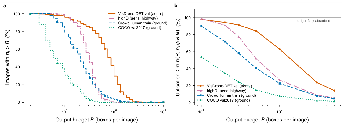
Figure 2.
Gain in worst-image recall from reallocating a fixed output budget, in percentage points. a, Gain against budget B for both prediction heads; faint crosses mark budgets above which the budget cannot be spent in full, so the two allocations coincide and the comparison is an identity rather than a measurement. The horizontal axis is the average per-image budget. b, The same comparison at the pre-specified budget fraction = 0.5, shown separately for the two prediction heads, so that its horizontal axis is the head and not the budget; only the extreme budgets of panel a are budget separations, and this panel is not one of them. N = 548 throughout; these are exact counts, so no error bars are shown. The curve was generated with the earlier matcher; at = 0.5 the plotted worst-image gains coincide with the corrected recomputation, but no other budget point has been recomputed with the corrected matcher.
Figure 2.
Gain in worst-image recall from reallocating a fixed output budget, in percentage points. a, Gain against budget B for both prediction heads; faint crosses mark budgets above which the budget cannot be spent in full, so the two allocations coincide and the comparison is an identity rather than a measurement. The horizontal axis is the average per-image budget. b, The same comparison at the pre-specified budget fraction = 0.5, shown separately for the two prediction heads, so that its horizontal axis is the head and not the budget; only the extreme budgets of panel a are budget separations, and this panel is not one of them. N = 548 throughout; these are exact counts, so no error bars are shown. The curve was generated with the earlier matcher; at = 0.5 the plotted worst-image gains coincide with the corrected recomputation, but no other budget point has been recomputed with the corrected matcher.
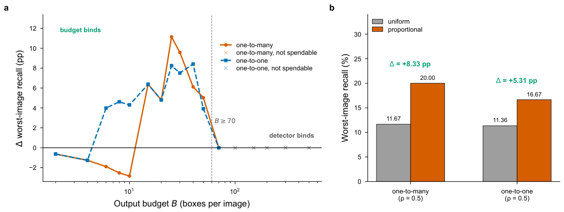
Figure 3.
What the reallocation does at the level of individual images. a, b, Per-image recall against object count under a uniform quota (grey) and proportional allocation (vermillion) at B = 25 and B = 70. Both panels are descriptive; budget-level degeneracy status is reported separately in Supplementary Table S10. Connectors join the two allocations for images whose recall changes by more than two points. Circles and squares mark the worst image under each allocation, labelled with its object count, quota and recall; a coloured outline means its quota reached the imposed label-count cap , not that the detector ran out of predictions. (The per-image ceiling equals throughout these records, because a prediction count below the annotated count never occurs; the outline condition is therefore the binding one.) Green crosses in b mark images that reached under both allocations yet stay below 45% recall, which is why, under this label-count-capped convention, the gain there is exactly zero. N = 548 in both panels. The panel was generated with the earlier matcher and is a historical, descriptive view; it has not been re-checked point by point under the corrected matcher.
Figure 3.
What the reallocation does at the level of individual images. a, b, Per-image recall against object count under a uniform quota (grey) and proportional allocation (vermillion) at B = 25 and B = 70. Both panels are descriptive; budget-level degeneracy status is reported separately in Supplementary Table S10. Connectors join the two allocations for images whose recall changes by more than two points. Circles and squares mark the worst image under each allocation, labelled with its object count, quota and recall; a coloured outline means its quota reached the imposed label-count cap , not that the detector ran out of predictions. (The per-image ceiling equals throughout these records, because a prediction count below the annotated count never occurs; the outline condition is therefore the binding one.) Green crosses in b mark images that reached under both allocations yet stay below 45% recall, which is why, under this label-count-capped convention, the gain there is exactly zero. N = 548 in both panels. The panel was generated with the earlier matcher and is a historical, descriptive view; it has not been re-checked point by point under the corrected matcher.
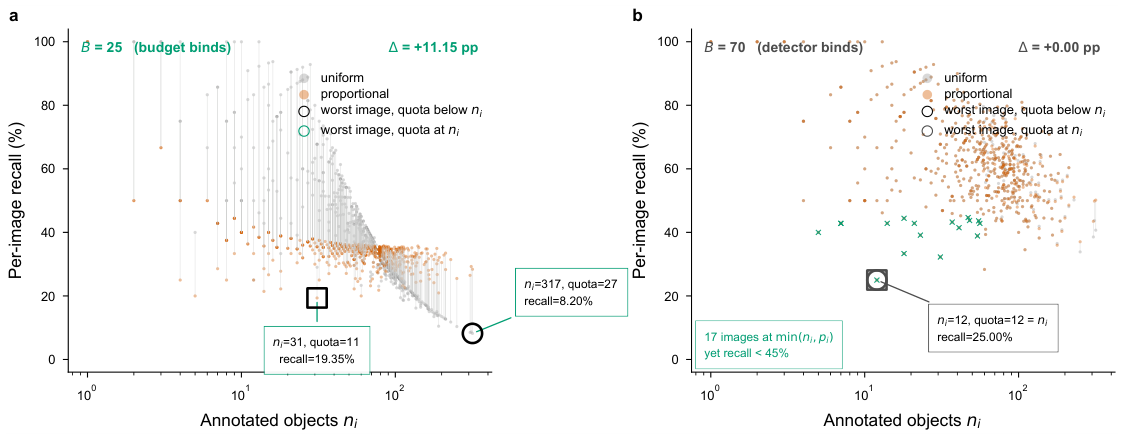
Figure 4.
The cost of the reallocation by object-count band. a, Change in per-image recall, proportional minus uniform, in percentage points, for each band; horizontal bars are 95% confidence intervals from a paired percentile bootstrap over images within the band (10,000 resamples; the RNG is derived per seed so that re-running one seed alone reproduces its row), and the vertical line marks zero change. Because the band boundaries are fixed by the label distribution, the interval estimates the mean cost of a band and not which images fall in it. Image counts per band are printed beside the labels. Colours and symbols follow Figure 2: circles for the one-to-many head, squares for the one-to-one head. b, Mean per-image recall under each allocation for the same bands; dashed connectors join the two allocations within a band, so the horizontal length of a connector is the change plotted in a. Grey circles mark the uniform allocation and vermillion triangles the proportional one. = 0.5, VisDrone validation, N = 548. Panel b shows the one-to-many head only; the one-to-one head appears in a. The panel was generated with the earlier matcher and is descriptive; the corrected recomputation differs by 0.01 points in the sparsest band and agrees to the reported precision in the densest one.
Figure 4.
The cost of the reallocation by object-count band. a, Change in per-image recall, proportional minus uniform, in percentage points, for each band; horizontal bars are 95% confidence intervals from a paired percentile bootstrap over images within the band (10,000 resamples; the RNG is derived per seed so that re-running one seed alone reproduces its row), and the vertical line marks zero change. Because the band boundaries are fixed by the label distribution, the interval estimates the mean cost of a band and not which images fall in it. Image counts per band are printed beside the labels. Colours and symbols follow Figure 2: circles for the one-to-many head, squares for the one-to-one head. b, Mean per-image recall under each allocation for the same bands; dashed connectors join the two allocations within a band, so the horizontal length of a connector is the change plotted in a. Grey circles mark the uniform allocation and vermillion triangles the proportional one. = 0.5, VisDrone validation, N = 548. Panel b shows the one-to-many head only; the one-to-one head appears in a. The panel was generated with the earlier matcher and is descriptive; the corrected recomputation differs by 0.01 points in the sparsest band and agrees to the reported precision in the densest one.
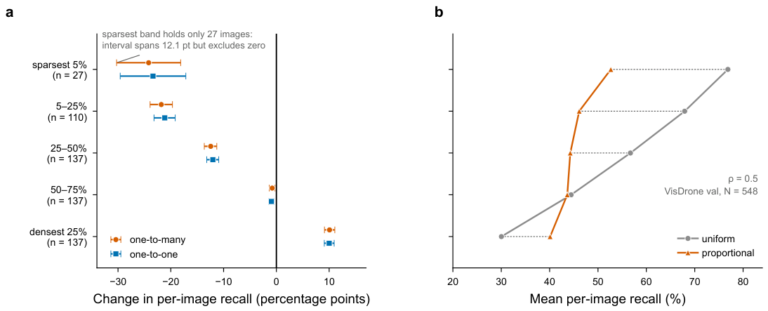
Figure 5.
Sparse images hold larger objects. a, Mean annotation-box area per image against the annotated object count , with the median per logarithmic count bin overlaid. b, Mean box area for the sparsest 5% of images (27 images, 1-9) and the densest 25% (137 images, 93-317), the same bands used in Figure 4; the number above each bar is the image count in that band. Areas are normalised (YOLO wh, as a fraction of image area), so no image dimension enters the statistic. The Spearman correlation between object count and mean box area is -0.4596, and the sparsest band’s mean box area is 19.62 times the densest band’s. This is why a per-image quota costs the sparse images most: when an image holds few but large objects, each box carries more of that image’s recall, so a proportional allocation that reclaims that image’s boxes removes more recall than the same number of boxes taken from a dense image with small objects. We deliberately do not infer object distance, because VisDrone carries no depth annotation.
Figure 5.
Sparse images hold larger objects. a, Mean annotation-box area per image against the annotated object count , with the median per logarithmic count bin overlaid. b, Mean box area for the sparsest 5% of images (27 images, 1-9) and the densest 25% (137 images, 93-317), the same bands used in Figure 4; the number above each bar is the image count in that band. Areas are normalised (YOLO wh, as a fraction of image area), so no image dimension enters the statistic. The Spearman correlation between object count and mean box area is -0.4596, and the sparsest band’s mean box area is 19.62 times the densest band’s. This is why a per-image quota costs the sparse images most: when an image holds few but large objects, each box carries more of that image’s recall, so a proportional allocation that reclaims that image’s boxes removes more recall than the same number of boxes taken from a dense image with small objects. We deliberately do not infer object distance, because VisDrone carries no depth annotation.
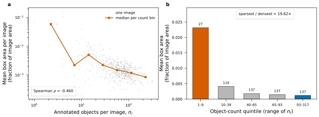
Figure 6.
Reallocation shifts the whole lower tail of the recall distribution. Quantile curves of per-image recall under uniform (blue) and proportional (orange) allocation at = 0.50, seed 42. a, one-to-many head. b, one-to-one head. The orange curve lies above the blue one below roughly the 35th percentile and below it between the 40th and 95th, so the gain is a property of the lower tail rather than of one image; the two allocations share the upper endpoint but their minimum recalls differ, because reallocation moves the minimum to a different image. Dotted verticals mark the minimum, 5th and 10th percentiles. N = 548 images per panel. Each curve is a quantile function of an exact per-image count, so no error bars are shown.
Figure 6.
Reallocation shifts the whole lower tail of the recall distribution. Quantile curves of per-image recall under uniform (blue) and proportional (orange) allocation at = 0.50, seed 42. a, one-to-many head. b, one-to-one head. The orange curve lies above the blue one below roughly the 35th percentile and below it between the 40th and 95th, so the gain is a property of the lower tail rather than of one image; the two allocations share the upper endpoint but their minimum recalls differ, because reallocation moves the minimum to a different image. Dotted verticals mark the minimum, 5th and 10th percentiles. N = 548 images per panel. Each curve is a quantile function of an exact per-image count, so no error bars are shown.
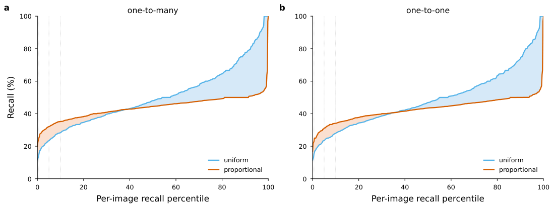
Disclaimer/Publisher’s Note: The statements, opinions and data contained in all publications are solely those of the individual author(s) and contributor(s) and not of MDPI and/or the editor(s). MDPI and/or the editor(s) disclaim responsibility for any injury to people or property resulting from any ideas, methods, instructions or products referred to in the content. |
© 2026 by the authors. Licensee MDPI, Basel, Switzerland. This article is an open access article distributed under the terms and conditions of the Creative Commons Attribution (CC BY) license (http://creativecommons.org/licenses/by/4.0/).
Copyright: This open access article is published under a Creative Commons CC BY 4.0 license, which permit the free download, distribution, and reuse, provided that the author and preprint are cited in any reuse.