

Submitted:
13 November 2026
Posted:
18 November 2026
You are already at the latest version
Abstract
Aging is a universal concept across complex systems. Like entropy, aging is anthropomorphic in that it belongs to the system specified by chosen defining properties rather than to a physical object. To understand aging from first principles, we reviewed definitions of aging and equivalent terms in 415 living and non-living systems and found that nearly all tie the change of a property to an internal state that changes with time, use or exposure. Adding the direction that separates aging from development and recovery, we define aging as the cumulative drift of a system’s internal state towards the boundary of the region of state space in which its defining emergent properties persist. Aging is therefore an emergent property of a complex system, and once the system is chosen, its dynamics decide whether and how fast it ages. A system can age only if regulation and renewal leave some slowly changing variable unrestored. Of four cases of drift towards a boundary, only weakening regulation both slows recovery from a small challenge and enlarges the response. For organisms, with death as the boundary and the distance from death as reserve, the definition specifies what biomarkers must track, rejuvenation must restore and negligible senescence must preserve.
Keywords:
aging
; senescence
; definition of aging
; complex systems
; state space
; resilience
; rejuvenation
; biomarkers of aging
1. The Problem of Defining Aging
Fields that study living and non-living systems describe them as aging or senescing (Supplementary Data 1), and each defines aging by the change of a property of the whole system. Battery engineers place a cell’s end of life where its capacity or peak power falls below 80% of its rated value; [?] limnologists describe the aging of a lake as the filling of its basin with sediment and organic matter until the lake gives way to marsh and dry land; [?] and seed scientists say that stored seeds age as they lose quality or viability over time. [1] Because each of these fields names the property it follows, it can say whether aging has occurred, how fast it proceeds and whether it has been reversed.
Biology, by contrast, has not agreed on which change defines organismal aging. The candidates include physiological integrity, fitness, the rate of mortality, a set of mechanisms and an accumulating deleteriome. [2]–5] Lemoine identified five features commonly used to define aging, from structural damage to an increasing probability of death, and found one consensual description, a process of loss characterized by a rate. [6] Surveys of aging researchers find no consensus either, and in a 2024 survey no question received a majority answer. [7,8] A definition is now needed because partial reprogramming and a young circulation are reported to rejuvenate human cells or mice, as measured by molecular clocks, omic profiles and selected functions. [9]–11] Whether a species senesces can be tested from its age patterns of mortality and fertility, which have been documented for many species, [12] but no agreed criterion specifies how to recognize rejuvenation or slowed aging in an individual. A meeting on gerophysics called for definitions of aging, rejuvenation and healthspan in terms of state variables. [13]
In the fields above, whether aging has occurred, how fast it proceeds and whether it has been reversed depend on which property defines the system whose aging is followed, a choice that biology has not made. Jaynes, crediting the remark to Wigner, wrote that “even at the purely phenomenological level, entropy is an anthropomorphic concept”, [14] because thermodynamics assigns entropy not to a physical system but to a thermodynamic system, defined by the macroscopic variables an experimenter chooses to measure or control, so one crystal has different entropies under different choices of variables. Aging is anthropomorphic in the same sense, because it belongs to the system specified by its defining properties rather than to a physical object, so one body can contain several systems that age differently. The ovary, defined by its fertility, reaches its boundary at menopause as its follicle pool is depleted, decades before the woman, defined by her life, reaches death (Figure 1a; Table 1). The choice is constrained, because a defining property must belong to the system as a whole and its loss must end that kind of system (Box 1, rule 1), whereas whether the chosen system ages, and how fast, follows from its dynamics. A definition of aging that holds across fields must therefore take the system and its defining properties from the field that studies it, or state them where the field has not, and specify only what the dynamics must do. For organisms we take the individual organism, defined by the maintenance of its life, as the system and death as its boundary.
Earlier accounts that compare aging in living and non-living systems disagree on whether the comparison holds. Hayflick noted that age changes occur in virtually all animate and inanimate matter, [15] whereas Golubev argues that inanimate things deteriorate but do not age, because they have no metabolism. [16] Reliability theory treats organisms and machines alike, defining aging as a failure rate that rises with age and showing that a redundant system built of non-aging parts ages as its parts fail and are not replaced. [17] Qin similarly proposes that aging arises at the level of biological networks whose components do not age, with aging defined as a mortality rate that rises over time. [?] Castorina and Blanchard place human aging and the aging of technical devices in one classification of growth laws, [18] and nuclear safety standards define aging for any structure, system or component as a gradual change of its characteristics with time or use. [?]
Other accounts describe a region of states within which a system must remain. Ashby defined an animal’s survival as keeping its essential variables within physiological limits and wrote that an animal that always did so could die only of old age. [19] Aubin’s viability theory asks which initial states allow a system to remain within a given set of constraints, [20,21] and Walker and colleagues call the closeness of a social–ecological system to a threshold its precariousness. [22] In biology, Rattan defines aging as the shrinkage of a living system’s homeodynamic space, [23] whereas Moldakozhayev and Gladyshev propose that homeostasis is reached only briefly and that the imperfect attempts to reach it generate damage whose accumulation drives aging. [24]
Models of mortality and reliability go further and place death or failure where a latent state reaches a boundary. In first-passage models death comes when a fluctuating physiological state first crosses a boundary, [25,26] and in threshold regression and degradation models failure comes when a path of degradation or health reaches a threshold, sometimes with trauma as a competing cause. [27]–29] Strehler and Mildvan place death where a challenge exceeds a vitality that declines with age. [30] Structural reliability expresses the distance of a design from its limit state as a reliability index, [31] and the theory of repairable systems expresses the effect of repair as a virtual age. [32] Software engineering counters software aging with rejuvenation, the restart of a long-running process at a clean internal state. [33]
In biology, dynamic-stability accounts tie aging to regulatory dynamics that are unstable or close to a loss of stability, [34,35] a complex-systems approach attributes it to the disruption of regulation integrated across scales [36] and a control-theoretic account defines it as a progressive loss of safe controllability. [37] Other accounts let the regulated state itself move: Dilman proposed a rising hypothalamic threshold to feedback control as a mechanism of aging, [38] allostasis is stability achieved through change [39] and Pridham and Rutenberg call the drift of aging organisms towards equilibria of worsening health mallostasis. [40] Studies of resilience read slower recovery from perturbations as a loss of resilience, [41]–43] which Ukraintseva and colleagues distinguish from robustness, the ability to resist a deviation from the baseline state rather than to recover after it. [44] The stochastic process model of human aging lets the optimal physiological state shift with age while adaptive capacity declines. [45]
Here we review the definitions and usages of aging, and of equivalent terms, in 415 living and non-living systems (Figure 1; Table 1; Supplementary Data 1) and find that nearly all share three elements: a property, an internal state and the change of that state with accumulated time, use or exposure. These elements and the direction of the change give a definition that, like the accounts above, describes a system by its internal state and by its defining properties. The internal state comprises the variables, such as composition, structure or stored energy, that together with the external conditions fix how the system will change, and the defining properties, such as an organism’s maintenance of its life, belong to the whole system and to no part alone and cease at the boundary of a region of internal states, a boundary that for an organism is death. To these accounts the definition adds the direction in which the state drifts relative to the boundary as a criterion that separates aging from other changes of state in every field. Aging carries the internal state towards the boundary, whereas development, recovery and adaptation, which also change the state with time, use or exposure, carry it away. Because the definition takes the kind of system, such as a battery cell, a lake or an organism, and its boundary from the field that studies the system, the boundary can also be a threshold or an equilibrium, unlike in dynamic-stability accounts. [35] In living and non-living systems alike, the definition separates measured quantities from the state they report, counts each change by what it leaves in the state rather than by its speed or source, and recognizes rejuvenation by comparing how the system afterwards drifts and responds with how a less aged one does (Box 1, rule 6). Supplementary Data 1 gives each field’s definition with its source.
Applied to the 328 systems whose fields call the change aging or senescence, the definition counts 291 (89%) as aging, 128 of them under a stated condition, which is most often a boundary that we declare because no document names an end. We then explain why complex systems so often age and compare the signatures of four cases of drift towards a boundary. Taking death as the boundary of an organism and the distance from death as its reserve, we state what biological age is and what each type of aging clock estimates, sort the ways in which lifespan can be extended and give criteria for the onset of aging, negligible senescence, slowed aging and rejuvenation. We also show that as regulation weakens, a regulated variable and its actuator, such as blood pressure and heart rate, can change their variance in opposite directions.
2. Survey of Definitions in 415 Systems
The survey covers 415 systems from 31 domains (Figure 1a; Table 1; Supplementary Table 1). The systems comprise 227 physical materials and devices, 66 natural systems (stars, planetary bodies, landforms, lakes, oceans, clouds and ecosystems), 86 living systems and stored biological materials, and 36 abstract and computational systems. In 328 systems the field calls the change aging or senescence, in 78 it uses another term, such as degradation, weathering, deactivation or spin-down, and in 9 it states that the system does not age.
We included a source only when it defines aging, or uses aging or a term for the same process, for a change in a named system (Methods), so every definition follows a property of that system, such as the hardness of an alloy or the mortality of an organism. In 395 definitions the change in that property is tied to an internal state, such as composition, structure or stored energy, fully in 348 and in part in 47 (Figure 1a), including 318 of the 328 systems whose fields call the change aging or senescence. The other 20 definitions name no internal change; their systems include a deployed prediction model with fixed weights whose accuracy falls (S243), a radioactive source whose surviving nuclei are unchanged as its activity falls (S124) and four organisms whose sources detected no decline (S213, S220, S221, S320). The counts below refer to the 395 definitions with an internal state, of which 217 are for physical materials and devices, 65 for natural systems, 81 for living systems and 32 for abstract and computational systems.
Figure 1.
Aging across living and non-living systems. a, Tree of the 415 surveyed systems, one definition each, in four groups and 31 domains. Ribbons scaled by the number of definitions run from the root to the groups and from the physical group to two subgroups, and each domain shows an example system, its number of definitions and a short name (full names in Supplementary Table 1). The schematic at top left shows the link that nearly every definition makes between an internal state that depends on accumulated time, use or exposure and a property of a chosen system, with one woman taken as two systems: her ovary, defined by its fertility, ends at menopause, and she, defined by her life, ends at death (the age axis has no scale). The stacked bar at bottom left divides the definitions into those that make the link between property and internal state fully (348), in part (47) or not at all (20) (Supplementary Figure 5b). Small plots beside nine domains show published time courses of a property in 13 systems. They show the enthalpy recovered by an aging polymer glass, [47] the hardness of a quenched Al–Cu–Mg alloy held at 170 °C (darker) and 105 °C (lighter), [48] the capacity of seven lithium-ion cells (the median-life cell darker) against cycle number with the 80% end of life (dashed) [?,49] and the relative count rate of a silver-111 sample. [50] They also show the Schmidt-hammer rebound of granite surfaces against exposure age with the published calibration curve, [51] the capacity of a reservoir as sediment fills it, [?] the luminosity and core hydrogen fraction of the Sun in a standard solar model, [52] aspartate isomerization in four lens-nucleus peptides against donor age [53] and the doubling time of old-pole (darker) and new-pole (lighter) E. coli lineages. [54] The remaining plots show the median grip strength [55] and annual death rates [?] of men (darker) and women (lighter) against age, the accuracy of a deep network over tasks learned in sequence, with a linear network for comparison, [56] and the duration of cloud-software jobs under load until the system fails (dashed). [?] Shading marks the change from a reference state (ring), and gray lines show the values before it. For the silver-111 sample the shading marks a fall in the number of surviving nuclei, which the definition does not count as aging. Horizontal axes show time, use or exposure, and no axis is numbered. The time axis of the polymer glass is logarithmic, and the silver-111 count rate and the death rates are plotted on logarithmic scales. The sources’ error bars are not drawn. A dagger marks cross-sectional data and an asterisk modeled values. The source data give every plotted value and how it was obtained. b, Lifetimes (discs) and process times (squares) of 28 systems against size (Supplementary Table 5). For each organism, marker style shows whether its sources have detected a decline (read from mortality or, for bristlecone pine, from its tissues), have detected none or have not measured one. [12,57]–59] The 238U and 14C nuclei, the free neutron and the 2p hydrogen atom are single units that end without aging (open circles), plotted at their own size and mean life. Shading marks where these mean lives overlap the lifetimes of aging systems, and the boxed region is enlarged at right. Tg is the glass transition temperature.
Figure 1.
Aging across living and non-living systems. a, Tree of the 415 surveyed systems, one definition each, in four groups and 31 domains. Ribbons scaled by the number of definitions run from the root to the groups and from the physical group to two subgroups, and each domain shows an example system, its number of definitions and a short name (full names in Supplementary Table 1). The schematic at top left shows the link that nearly every definition makes between an internal state that depends on accumulated time, use or exposure and a property of a chosen system, with one woman taken as two systems: her ovary, defined by its fertility, ends at menopause, and she, defined by her life, ends at death (the age axis has no scale). The stacked bar at bottom left divides the definitions into those that make the link between property and internal state fully (348), in part (47) or not at all (20) (Supplementary Figure 5b). Small plots beside nine domains show published time courses of a property in 13 systems. They show the enthalpy recovered by an aging polymer glass, [47] the hardness of a quenched Al–Cu–Mg alloy held at 170 °C (darker) and 105 °C (lighter), [48] the capacity of seven lithium-ion cells (the median-life cell darker) against cycle number with the 80% end of life (dashed) [?,49] and the relative count rate of a silver-111 sample. [50] They also show the Schmidt-hammer rebound of granite surfaces against exposure age with the published calibration curve, [51] the capacity of a reservoir as sediment fills it, [?] the luminosity and core hydrogen fraction of the Sun in a standard solar model, [52] aspartate isomerization in four lens-nucleus peptides against donor age [53] and the doubling time of old-pole (darker) and new-pole (lighter) E. coli lineages. [54] The remaining plots show the median grip strength [55] and annual death rates [?] of men (darker) and women (lighter) against age, the accuracy of a deep network over tasks learned in sequence, with a linear network for comparison, [56] and the duration of cloud-software jobs under load until the system fails (dashed). [?] Shading marks the change from a reference state (ring), and gray lines show the values before it. For the silver-111 sample the shading marks a fall in the number of surviving nuclei, which the definition does not count as aging. Horizontal axes show time, use or exposure, and no axis is numbered. The time axis of the polymer glass is logarithmic, and the silver-111 count rate and the death rates are plotted on logarithmic scales. The sources’ error bars are not drawn. A dagger marks cross-sectional data and an asterisk modeled values. The source data give every plotted value and how it was obtained. b, Lifetimes (discs) and process times (squares) of 28 systems against size (Supplementary Table 5). For each organism, marker style shows whether its sources have detected a decline (read from mortality or, for bristlecone pine, from its tissues), have detected none or have not measured one. [12,57]–59] The 238U and 14C nuclei, the free neutron and the 2p hydrogen atom are single units that end without aging (open circles), plotted at their own size and mean life. Shading marks where these mean lives overlap the lifetimes of aging systems, and the boxed region is enlarged at right. Tg is the glass transition temperature.
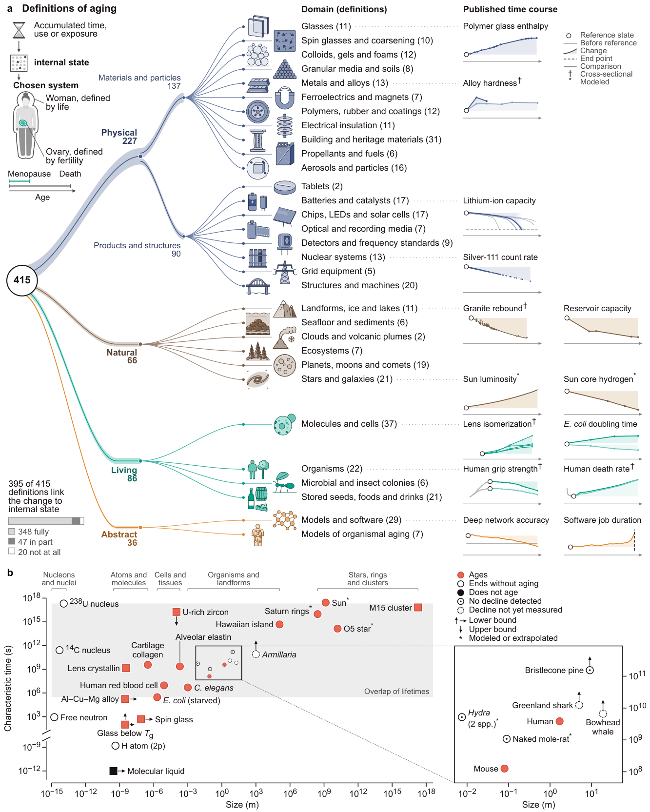

Table 1.
Definitions of aging in 12 of the 31 domains.
| Domain (n) | Property followed and internal change | Boundary or threshold named |
|---|---|---|
| Glasses and amorphous solids (11) | Relaxation times of a polymer glass as frozen-in excess volume and enthalpy relax (S001) | Equilibrium; heating above the glass transition erases aging (S003) |
| Metals and alloys (13) | Hardness of a quenched alloy as solute leaves the supersaturated solution (S030) | Equilibrium, which ends the quenched state (S030) |
| Capacitors, batteries, fuel cells and catalysts (17) | Capacity and power of a lithium-ion cell as side reactions consume cyclable lithium and active material is lost (S106) | Peak power and energy below test targets (S106) |
| Semiconductor and optoelectronic devices (17) | Luminance of an organic light-emitting diode as emitter and host molecules react (S097) | 50% of initial luminance (S097) |
| Engineered structures, machines and reliability (20) | Residual strength of an airframe as fatigue cracks grow and link (S188) | A residual-strength requirement and a limit of validity in flight cycles (S188) |
| Landforms, ice, lithosphere and lakes (11) | Persistence of a lake as sediment fills its basin (S244) | A filled basin (S244) |
| Planetary bodies and surfaces (19) | Activity of a comet nucleus as volatile ice is lost behind a dust mantle (S163) | A dormant or dead comet (S165) |
| Stars, compact objects and galaxies (21) | Core hydrogen burning of a main-sequence star as core hydrogen is consumed (S169) | End of core hydrogen burning (S169) |
| Molecules, organelles, cells and tissues (37) | Transparency of the lens as crystallins are modified (S195); fertility as the follicle pool is depleted (S209) | Cataract (S195); menopause (S209) |
| Organisms (22) | Physiological integrity and vulnerability to death of mammals as molecular and cellular damage accumulates (S212) | Death, with no numeric threshold (S212) |
| Stored biological materials and foods (21) | Viability of stored seed as oxidative damage builds up in its glassy cytoplasm (S224) | Regeneration at 85% of initial viability (S224) |
| Models and software (29) | Ability of a continually trained network to learn new tasks as its units go dormant (S242) | Learning no better than a shallow network (S242) |
In 380 of the 395, the state changes gradually with accumulated time, use or exposure. Nine give no time course, and in six a single event changes the state (for example, S312). The property can rise or fall. Static friction grows with the time two surfaces stay in contact (S027), the hardness of a quenched alloy rises and then falls (S030, S031) and the capacity of a battery cell falls (S105). Several sources state that elapsed time does not cause the change. Oscillator aging is the change of frequency “due to internal changes in the oscillator”. [?] The American Concrete Institute writes that aging, “if one means merely the effect caused by the passage of time, has no effect on concrete”. [?] For stars, Soderblom writes that “age is not the direct agent of that change”. [46] Many definitions count use in place of time, such as charge–discharge cycles (S106), flight cycles (S188), perihelion passages (S164) or population doublings (S204).
Fields add three conditions to the shared elements (Supplementary Figure 5a). A threshold or standard is named in 182 definitions (46.1%), such as peak power and energy below test targets for a battery cell (S106) and 85% of initial viability for seed in a genebank (S224). Some sources treat their threshold as a convention, and Koerner and colleagues call the 50% criterion for geomembranes “quite arbitrary”. [?] A dependence on the time since the system formed or was last reset is required in 243 (61.5%). The two-time functions of glass physics count time from the quench (S013, S016), and reheating a glass above its glass transition erases its aging (S001). A loss of performance or function is required in 145 (36.7%), or in 42.3% if the 22 that are unclear on this point are counted. Forty-eight definitions (12.2%) add none of the three conditions.
Whether aging must be a loss differs between groups. A loss is required by 40.6% of the definitions of physical materials and devices (88 of 217), 51.9% of living-system definitions (42 of 81), 37.5% of abstract and computational ones (12 of 32) and 4.6% of natural-system definitions (3 of 65). The three natural cases are all ecological (S145, S286, S288), so no definition of a landform, planetary body or star requires a loss. In the living group, a loss is required in 13 of 17 definitions for organisms and 6 of 21 for stored biological materials and foods, where cheese, wine and whisky are aged to improve them (S226, S227, S231).
3. Change of a Property in 13 Systems
Beside nine of the domains in Figure 1a we replotted published measurements of a property in 12 systems, chosen from the four groups to differ in scale and field, together with the Sun as a standard solar model describes it (Supplementary Note 4, S15). Glass physics measures aging by two-time functions, in which a correlation or response is followed over a lag that starts at a waiting time after the quench, and an equilibrium liquid does not age. [60]–62] Polymer science often follows one-time readouts of this physical aging, such as the enthalpy recovered on reheating. [47,63] Metallurgists follow the hardness of a quenched alloy, and battery engineers follow the capacity of lithium-ion cells against an end of life at 80% of rated capacity (Figure 1a). [?,48,49] By contrast, radiochemistry calls the loss of parent nuclei decay and describes it by a constant that does not change in time (Figure 1a), [?,50,64] and studies of nuclear materials speak of aging where decay changes the function of a material, as in plutonium. [65] Astrophysicists speak of aging for the evolution of a star’s internal state, [46] and the Sun’s luminosity has risen as its central hydrogen fraction has fallen (Figure 1a). [52,66]
Geomorphologists date granite surfaces by their Schmidt-hammer rebound, which falls as weathering loosens the surface grains, [51] and the storage capacity of a reservoir falls as sediment fills it (Figure 1a). [?] A deep network trained on a long sequence of tasks loses its ability to learn each new task until its accuracy falls below that of a linear network. [56] Software aging is the accumulation of errors, such as leaked memory, unreleased locks and fragmented storage, in the state of a long-running process (S241), and in an OpenStack deployment under load the duration of a job rises until the system fails (Figure 1a). [?]
Few of the plotted measurements from organisms follow individuals (Figure 1a). The doubling time of old-pole E. coli lineages, which are followed through successive cells, lengthens and then settles while that of new-pole lineages shortens. [54] The proteins of the human lens nucleus accumulate isomerized aspartate without turnover, as comparisons across donors show, [53] and human grip strength and death rates are likewise mostly known from comparisons of people of different ages. [?,55]
Measured from a reference state, the property rises in some systems and falls in others (Figure 1a). The same alloy held at two temperatures follows two courses over the same days, so elapsed time alone does not fix its state. Four of the plotted systems measure age by use and five compare people, surfaces or specimens of different ages, and only two mark an end point on the plotted readout. Systems of similar size or lifetime also differ in whether and how they age (Figure 1b). The mean lives of single 238U and 14C nuclei, which end without aging, lie among the lifetimes of systems that age, and organisms of similar size differ in their reported mortality patterns.
4. A Definition of Aging
The three shared elements do not separate aging from other changes of state, because development, recovery from an injury and the fluctuations of a system at equilibrium also change a property through the internal state. Aging differs from these changes in its direction, because in aging the internal state drifts towards the boundary where the defining property ceases, whereas development and recovery carry it away from that boundary. Summarizing the shared elements with this direction gives the following definition:
Aging is the cumulative drift of a system’s internal state towards the boundary of the region of state space in which its defining emergent properties persist.
In a lithium-ion cell, the field follows capacity and places the end of life at 80% of rated capacity, so that threshold is the cell’s boundary. [?] The cell’s internal state includes the inventory of cyclable lithium, which side reactions consume and charging does not restore. [67,68] Its margin, the distance of the state from the boundary, falls as the cell ages and, when cyclable lithium limits capacity, is the cyclable lithium above the inventory at end of life.
In general, the internal state comprises the variables whose present values, together with the external conditions, fix the system’s future. The defining properties are emergent in that they belong to the system at the level at which it is described and to no constituent alone. [69] Because aging is the drift of the state relative to the region in which these properties persist, it is itself an emergent property of the system. The system is whatever its field studies at that level, which may be a whole object or a part, such as a battery cell in a pack or the weathered surface of a rock. A part can be a system in its own right with its own boundary, so a cell of an embryo can die by apoptosis while the embryo develops. Which system to follow and which of its properties count as defining is the anthropomorphic choice discussed in the opening section (Box 1, rule 1).
The region is the set of states in which the defining properties hold, and the boundary is the set at which they cease. A field or standard can fix the boundary as a threshold, as for the battery cell, or the boundary can lie where the system’s own dynamics lose stability or reach equilibrium. Moving such a threshold changes when the system ends but not the direction of its drift (Supplementary Note 4, S7.6), and a change of external conditions can also move the boundary. The region and its boundary can be drawn on a quasi-potential, a surface whose height is set by the dynamics and whose wells are the stable states (Figure 2a).
Measured quantities such as hardness are readouts, which depend on the state and can rise while the state drifts towards the boundary, as the hardness of a quenched alloy does while precipitation carries the alloy towards the equilibrium that ends the quenched state (Figure 1a). We instead follow the drift through the margin, which is zero on the boundary and positive inside the region. The margin depends on the slow variables, such as composition, damage, stores and set points, which change much more slowly than the rest of the state. The margin is defined from the variables that the field measures, before the drift is observed, and a proposed margin fails if, among systems of the same age, those that it places closer to the boundary reach the boundary on average later (Box 1, rule 3).
Drift is the rate at which the margin changes once the fast fluctuations of the state are averaged out (Box 1, rule 4). For example, the state of charge of a battery cell rises and falls with every cycle, while its cyclable lithium falls, and only the fall of cyclable lithium is drift. Negative drift is aging, and positive drift is formation, which in an organism is development (Box 1, rule 5). A system whose margin falls on average ages even when its slow variables are noisy, whereas a margin that only diffuses, rising and falling at random with no trend, has zero drift. Undirected steps in the slow variables, by contrast, lower the margin on average around its maximum and so give negative drift (Supplementary Note 4, S3.1). Drift is cumulative because the state retains the effect of each step, and the rate at which a stated measure of the margin is lost is the rate of aging.
A large fluctuation, an accident or a hazard that does not depend on the state can carry a system across the boundary while its margin is still positive. Such a crossing, which we call an event, ends the system without being drift, whereas whatever a shock leaves in the slow variables of a system that survives it, such as lasting damage, enters the drift as any other step does (Box 1, rule 4). A rise of the margin driven from outside is rejuvenation when it returns the drifted slow variables towards their earlier values and adaptation when it raises the margin through other slow variables (Box 1, rule 6). On the quasi-potential, aging lies beside formation, rejuvenation, adaptation, stationarity, the crossing of the boundary and the abrupt end of a metastable state (Figure 2a; Supplementary Figure 1; Supplementary Table 10).
Whether drift is a loss is a separate judgment against a standard. Engineers judge loss against what users need, and organismal definitions judge it against function or survival [?] and sometimes against fertility. [4] The same drift can be a loss under one standard and not under another, so the definition leaves the judgment of loss out. A threshold that users set, such as the 80% end of life of a battery cell, still places a boundary, and an outcome of the definition that rests on it carries their standard. Lemoine’s process of loss characterized by a rate [6] is the drift with a standard of loss added.
The defining properties depend on the kind of system that a field studies, and we take the kind that the field gives (Box 1, rule 1). Fields that study a prepared nonequilibrium state, such as glass physics, take that state as the kind, and its boundary is equilibrium (Box 1, rule 2). The system is then the prepared state, so reaching equilibrium ends it even though the material is then more stable. A glass ends at equilibrium with the supercooled liquid, and its margin is the departure of its structure from that of the supercooled liquid at the same temperature, [63,70] which shrinks as the glass ages and vanishes at equilibrium. A glass, a spin glass or a frictional contact therefore ages while its relaxation slows and its stiffness, order or static friction rises. Aging can thus raise a system’s stability when its boundary is an equilibrium that its own dynamics approach.
The kind of system also determines when a glass counts as rejuvenated. After large stresses below yield, the mechanical response of a polymer glass looks rejuvenated while its volume recovery is unaffected, and whether such stresses rejuvenate the glass has been disputed. [71] With the glass as the kind, a stressed glass is rejuvenated only if its structure has returned towards that of a less aged glass, so that it then drifts and responds as that glass does (Box 1, rule 6). Because volume recovery follows the structure and is unchanged, the stress has not rejuvenated the glass. A field that took the mechanical response as the defining property would judge the stress by the later course of that response, and with the kinds stated the two fields can say where they differ (Supplementary Table 8).
5. The Definition Applied Across Systems
We applied the definition to each surveyed system by a fixed rule (Methods) and compared the outcome with the field’s own term. Of the 328 systems whose fields call the change aging or senescence, the definition counts 163 as aging, 128 as aging under a condition, 23 as formation and 12 as not aging, and it leaves one outcome mixed and one undetermined. Aging with or without a condition thus covers 291 of the 328 (89%). Of the 128 outcomes of aging under a condition, 66 rest on a boundary that we declare, because no document names an end. In the other 62, each counted by its first unmet condition, the source leaves the direction unstated (24), names the internal state only in part (20), follows a property that rises and then falls or levels off while the kind persists (15), gives no time course (1) or follows fertility, a property of a reproductive part (2; S219, S319). The undetermined outcome is sealed gasoline, in which no decline was detected over the 12 months of the study, so the finding sets an upper bound on the rate of aging and leaves open whether the gasoline ages (S339). The 23 formation outcomes carry the state into the region where the defining property holds or deeper into it, as in the hardening of young concrete, the manufacturing aging of lithium-ion cells and the maturation of cheese and wine. Of the 12 systems counted as not aging, nine have definitions that name no internal change, such as lifetime distributions and a deployed prediction model whose weights are fixed. In one, the color change of stone patina does not bear on the stone’s integrity, and in two the change is a single event (the entry of a cell into the senescent state and the aging of an inhibited enzyme). The mixed outcome is senescence across 46 species, which differs among them (S216). Supplementary Data 1 gives the outcome and its reasons for every system.
Pairs of systems that differ in one respect show that whether a system ages depends on whether its state is stationary, how its parts are organized and whether it draws on a store that nothing refills (Figure 2b). The same substance does not age as a liquid at equilibrium, whose molecules move without changing the statistics of their arrangement, and ages once quenched below its glass transition, because the glass relaxes towards the equilibrium at which it would no longer be a glass. Units with a constant hazard, such as nuclei, do not age, because a surviving unit is in the same state as a new one, and each ends in a single event. Wired in series, such units form a system that fails at the first unit failure and so ends without aging. Wired in parallel, the same units form a system that works while any unit works and ages as it uses up its spares (Figure 2b). [17] More generally, any coherent system of independent units with constant hazards has a failure rate, averaged from age zero, that never falls with age. [72] A flame fed from a gas line burns unchanged for as long as the gas arrives, whereas a candle carries its own fuel and ages as its wax runs down. On the quasi-potential, the equilibrium liquid and the gas flame rest at a stable minimum, the nucleus and the series system end in one crossing, and the glass, the parallel system and the candle drift towards the boundary (Figure 2a; Supplementary Figure 2).
A collection of units that do not age therefore ages only through how its parts are organized or act on one another. The parent content of a radioactive sample falls at a constant fractional rate, as the size of a cohort of animals that die at a constant rate does. Each fall counts the surviving units, and a sample freed of its daughters is in the same state as a fresh, smaller one, so neither fall is aging, as radiochemistry holds (Figure 1a). Plutonium metal ages, although none of its nuclei do, because the products of decay stay in its lattice and change it. [65] In organismal biology the kind is the individual organism, so the shrinking of a cohort does not show whether its members age (Box 1, rule 1; Supplementary Note 4, S3.4).
6. How Drift Reaches the Boundary
When the slow variables change much more slowly than the fast ones and noise is small (Box 2), a system can age only through slow variables that neither regulation nor renewal holds stationary under the stated conditions (Box 2, step 2). These variables include stores that are drawn down, such as the supersaturation of a quenched alloy, the core hydrogen of a star, the cyclable lithium of a battery cell and the spare units of a redundant system; [17] burdens that accumulate, such as fatigue cracks and the sediment in a lake basin; and settings that shift, such as the set points of regulated physiology (Supplementary Table 7; Supplementary Data 1, row S244). In a battery cell, growth of the solid–electrolyte interphase consumes cyclable lithium during storage, and lithium plating and loss of active material add to the loss of capacity during use (Figure 1a). [67,68] A restoring process can itself draw on a store, as when low-molecular-weight siloxanes that diffuse from the bulk restore the surface hydrophobicity of a silicone insulator, which ages as that reservoir is spent. [73] A reset from outside returns the drifted state towards its earlier values, as when a merger mixes fresh hydrogen into a star’s core. [74]
Complex systems so often carry such an unrestored slow variable because each slow variable needs a restoring process, and the more slow variables a system has, the harder it is to hold all of them. Perturbations that nothing corrects move the state away from where it started, and in three or more dimensions a random walk need not return. [75] A random change of a given size to a configuration that persists because it is tuned lowers the margin more often than it raises it, the more so the more variables the configuration has. [76,77] An unrestored slow variable can therefore give negative drift even when its steps have no preferred direction, where the margin is largest at the formed state and every direction leads downward from there, so that random spread of the state lowers the margin on average (Figure 2e; Supplementary Note 4, S3.1).
Drift of these slow variables reaches the boundary in one of three ways. A regulated state of the fast variables can lose stability, as when the gain of a regulatory loop (the strength with which its feedback opposes a deviation) falls towards a fold, the point at which the well disappears. A slow variable can cross a threshold while the fast state stays stable, as when the store of cyclable lithium in a battery cell runs down until its capacity falls below 80% of its rated value. A prepared nonequilibrium state can relax to equilibrium, as a glass does. The second way includes two cases, one in which the slow variable sets how far a given load moves the state, as the number of intact springs does when springs that share a load break at random, and another in which a set point drifts towards a failure value. Near a stable state and at fixed damping, the time to recover from a small perturbation, the response to a small push and the variance of fluctuations at fixed noise intensity all vary as the inverse of one restoring rate, which is proportional to the curvature of the well (Box 2, steps 6 and 8). We compare the four cases on these measures and on the hazard (Figure 2c,d).
Approaching a loss of stability slows recovery, raises the variance [78,79] and enlarges the response to a small push at the frequency of the slowest mode (a constant push near a fold). Resilience theory measures persistence by the size of the domain of attraction, [80] and physiology probes resilience with stimulus–response tests. [81,82] A store that sets sensitivity raises the response, the variance and the hazard as it runs down, [17,83] whereas recovery is unchanged (Supplementary Note 4, S16). A set point that drifts at constant gain raises only the hazard. A glass relaxes more slowly the longer it has aged, while its response to a small push and its rate of escape from its present configuration fall. [60,84] Walker and colleagues distinguish the resistance of a state (how hard it is to change) from its precariousness (its closeness to a threshold). [22] As a glass ages its resistance rises, and its precariousness grows because its margin shrinks. Slower recovery alone therefore fits a glass as well, and a larger response alone fits a store that sets sensitivity, so among the four cases only the approach to a loss of stability gives both.
Studies of abrupt climate change have tested part of this signature. Rising autocorrelation before eight abrupt climate shifts of the past [85] bears on the slower recovery but not on the larger response. Of the three routes to tipping that Ashwin and colleagues distinguish (through a bifurcation, through noise and through a change too fast for the state to follow), only the first requires a loss of stability. [86] Ditlevsen and Johnsen found no significant rise in variance or autocorrelation before the Dansgaard–Oeschger warmings of the last glacial period and concluded that noise probably induced them, [87] so each would be an event. However, read from the fluctuations of a single record, trends in variance or autocorrelation often detect an approaching fold no better than chance. [88]
7. Consequences for Organisms and Humans
Accounts of biological autonomy define an organism by its self-maintenance, through which it produces, repairs and regulates its own organization far from equilibrium. [89] We take an organism’s defining property to be maintaining its life (Supplementary Table 6). Its boundary is then death, [90] and its margin, which we call reserve, is the distance of its state from death in the variables that the field measures. Under this kind a decline in reproduction is aging of a part, whereas definitions that take fitness, which combines survival and reproduction, as the defining property choose another kind, under which it is aging of the whole (Supplementary Note 4, S7.5). Drift towards death is aging whatever disease or mechanism produces it, [91,92] including the loss of reserve that an illness builds up in childhood. When an acute infection or an injury leaves lasting damage, that damage lowers reserve and is aging, whereas a death that comes while reserve remains is an event, which ends the organism without being aging of it (Box 1, rule 4). Senescence is the species-typical part of this aging, the part that meets Strehler’s criteria of universality, intrinsicality, progressiveness and deleteriousness. [?]
Which measurements track reserve depends on how the organism approaches death. In adult humans, negative feedback holds regulated variables such as blood glucose, blood pressure and core temperature near set points, each at the bottom of a well whose curvature is set by the gain of regulation (Figure 2c). If the gain falls, the well flattens towards a loss of stability, and regulated variables recover more slowly from a small standard challenge and respond more strongly to it. They also fluctuate more if the random disturbances acting on them keep the same strength, but recovery and response do not depend on that strength and so track reserve. If set points instead drift towards a failure value at constant gain, the well moves towards the boundary with its shape unchanged, so recovery and response stay the same and only the distance of the set points from their failure values shows the drift.
Observations in humans are consistent with both a falling gain and drifting set points. The autocorrelation time of a state index derived from repeated blood counts was longer in older age groups of non-frail adults aged 40 to 90, as was that of daily step counts in a separate cohort aged 20 to 85. [43] After standing, blood pressure took longer to reach a steady value in older age groups. [93] Among women aged 84 to 95 with similar fasting glucose, the response to a glucose load was larger and more prolonged in frail individuals. [94] Both challenges are large and both comparisons are between groups, so they bear on falling gain only indirectly. In two human and two mouse cohorts, a model with recovery rates held constant across ages attributed age-related decline to drift in the equilibrium values of a few variables, [40] consistent with the pattern that set-point drift predicts.
Heart rate opposes disturbances of blood pressure, so blood pressure is the regulated variable of this loop and heart rate its actuator. As the gain of the loop falls, blood pressure recovers more slowly and fluctuates more. Heart rate, whose fluctuations are those of blood pressure multiplied by the gain, fluctuates less because the fall in gain outweighs the rise in the fluctuations of blood pressure, provided that blood pressure would return to its set point without the feedback. If only the feedback holds blood pressure there, heart-rate variability falls while the gain is high and rises again close to the boundary, where the variance of blood pressure diverges (Supplementary Figure 6; Box 2, step 8). Heart-rate variability does fall with age, [95] a decline that Lipsitz and Goldberger interpreted as a loss of complexity. [96] However, a lower vagal tone can reduce heart-rate variability without any change of gain, and the derivation leaves out the autonomic and respiratory noise acting directly on heart rate, so a test of falling gain must also show slower recovery of blood pressure in the same people. Rector and colleagues concluded that indicators of resilience must match the homeostatic role of the monitored variable, [97] and the derivation shows how studies that pool regulated variables with actuators can report opposite trends.
An organism begins to age when its reserve starts to fall, after development has raised it to a peak at the end of formation (Figure 3a,c). A fall of reserve during development, as in a childhood illness, is aging over its own window, and the onset refers to the fall of reserve after its peak. Aging defined as any change over time is fastest in the fetus, [98] but our definition counts that change as development, as Vaupel and colleagues do for the fall of mortality from conception to puberty. [99] Parts can age while the organism develops. The thymic epithelium shrinks from the first year of life, [100] and the never-replaced proteins of the lens nucleus already carry isomerized aspartate at 18 years, the youngest donor age in Figure 1a. [53] Almost half of 103 aging researchers placed the onset of human aging at gametogenesis, conception or gastrulation, [8] events that can begin the aging of germ cells and embryonic parts. Because reserve depends on all slow variables, growth and maturation can outweigh molecular damage and the processes grouped as hallmarks, so reserve can rise while damage accumulates (Supplementary Note 4, S3.1), and measures that weigh growth and damage differently place the peak at different ages. The onset is therefore stated relative to a named measure of reserve.
Evolutionary theories explain why reserve falls after formation. Because the force of natural selection falls with age, [?,103] alleles with harmful late effects can accumulate or persist for their early benefits, [104] and selection can favor saving on the maintenance of somatic cells. [105,106]
Because history affects the future only through the present state, a biomarker of aging must capture that state, and once it does, chronological age adds nothing to its prediction of the time to death in a stated environment. We call such a measurement a coordinate of the state. Chronological age cannot be part of a coordinate, because organisms in the same state can differ in age. Existing criteria instead ask whether a biomarker predicts functional capability [107] or outcomes such as mortality [108] better than chronological age. Criteria of the second kind also require a strong but imperfect correlation with chronological age. Klemera and Doubal derive biological age from the relationships between biomarkers and chronological age, with chronological age itself as one of the biomarkers. [109]
The definition also states what biological age is and what each type of aging clock estimates (Figure 3b). An organism’s biological age is the age at which the median reserve of the living members of a stated reference cohort, read after its peak, first equals the organism’s reserve. This median reaches the boundary only as the last members of the cohort die (Figure 3c). Biological age is thus reserve expressed in years, and it is unchanged by any order-preserving rescaling of reserve, which changes the median and the organism’s reserve alike. Where the state sets the risk of death through reserve, the same biological age means the same current risk of death in a stated environment. Biological age is the reserve counterpart of the equivalent ages that match biomarker values in the Klemera–Doubal method, [109] the risk of death in phenotypic age, [110] remaining life expectancy in the prospective age of demography [111,112] and the failure behavior of a repaired unit in the virtual age of reliability theory. [32] Clocks trained on chronological age [113,114] estimate elapsed time from the state. Training on age rewards features that change at the same rate in everyone, and such features carry no information about differences in reserve (Supplementary Figure 7). As the training sample of one such clock grew and its prediction of age improved, its association with mortality weakened. [115] By contrast, clocks trained on a mortality-based phenotypic age [110] or on time to death [116] estimate how close the state is to the boundary and, expressed in years against a reference cohort, approximate biological age. Both, however, take chronological age into their training target or inputs, so they cannot be assumed to be coordinates of the state.
Biological age corresponds to a position and the rate of aging to a speed. [108] Clocks trained on the within-person rate of change of physiological measures, such as 19 measures followed from age 26 to 45, [101] estimate the speed of drift, which under the definition is the rate of aging. Together, position and speed set the time left, which for a steady drift is the reserve divided by its rate of loss, so two people of the same biological age who age at different speeds die, on average, at different times (Figure 3d). Clocks built only from methylation sites whose causal effects on aging-related traits were estimated by Mendelian randomization separate the age-related changes that carry the state towards the boundary from those that carry it away. [102]
Most present measures capture only part of the state or resistance to particular challenges. For example, in older Canadians, chronological age remained associated with death after adjustment for a frailty-based biological age, [117] so that measure misses part of the state. In the Dunedin Study, 11 measures of biological aging agreed poorly and only some were consistently related to aging-related outcomes. [118] A partial measure, such as a DNA methylation clock, bears on reserve only where, among people of the same chronological age, those it places closer to death die on average sooner than the others.
An age read from one omic layer or one organ is the state projected onto the variables measured in that layer or organ, expressed in years, so the omic and organ ages of one person need not agree. Ages estimated from plasma proteins of organ origin differed between the 11 organs of the same individuals, and an accelerated age of an organ was associated with disease of that organ and with mortality. [119] Normative models built from imaging and physiological measures of three brain and seven body systems reported that the biological age of one organ system influences the aging of others. [120] Each such age follows the drift of a part, which bears on the organism’s reserve through the causes of death that arise in that part, and a layer that turns over within hours or days also carries fluctuations that a single sample cannot separate from drift. An omic or organ age is therefore the organism’s biological age only where it measures the organism’s reserve, and otherwise it measures the aging of a part (Figure 3c).
A species shows negligible senescence if the reserve of its members shows no species-typical fall after development. Renewal that holds every slow variable at a stable value is sufficient (Box 2, step 2), but compensating changes such as growth can also hold reserve level, so the claim must rest on reserve itself. A stationary readout, such as the settled doubling time of old-pole E. coli lineages (Figure 1a), [54] or a flat hazard among individuals compared at the same state bounds the rate of aging without showing that it is zero. The sources for the planarian Schmidtea polychroa and the germ line of Caenorhabditis elegans attribute the absence of a detectable decline to cell renewal and to rejuvenation of the lineage, respectively (Supplementary Data 1, rows S320 and S306).
A flat death rate in a cohort does not show that its members do not age, because the definition concerns the state of each individual, whereas demographic definitions rest on cohort hazards. Vaupel and colleagues define senescence as death rates that rise with age and call it negligible when they rise very slowly if at all and negative when they fall after reproductive maturity. [99] Baudisch measures the pace and shape of mortality on cohorts, [121] and Rose and colleagues interpret a leveling cohort death rate as evidence that individuals stop aging. [3] Yet when Proschan pooled airplane air-conditioning systems that each failed at a constant rate, the pooled failure rate fell, because the units with higher rates failed first. [122] In a human cohort, the early death of frailer members likewise makes the death rate rise more slowly than individual hazards. [123] Differences between age groups mislead in the same way. APOE ε4 is rarer in centenarians than in younger adults, although no one’s genotype changes, [124] and the cross-sectional curves of Figure 1a bear on individual aging only where within-person slopes agree with them. Drift must therefore be measured in the same individuals compared at the same state, or from failure rates stratified by state (Box 1, rule 7). Drift depends only on the present state, so the death of some members before a measurement does not change the drift at any state. Comparisons matched on the state therefore need no correction for selective loss, provided the measurements used to match states are coordinates of the state and successive measurements are close together compared with the time to death (Box 1, rule 5).
An individual’s hazard also follows from its state. With noise, death comes by escape over the barrier of the well. Near a fold the barrier falls as the well flattens, so the hazard rises as recovery slows (Box 2, step 7). A Gompertz rise in cohort mortality [125] can follow from a constant loss of vitality against exponentially distributed challenges, [30] from regulatory networks that are unstable or close to a loss of stability, [?,34,126] from removal of senescent cells that slows with age [127] and from the exhaustion of redundant elements. [17] A mortality curve alone therefore does not show how the state approached death. An accident can end a life while reserve remains positive and so counts as an event, and a state-independent hazard, such as Makeham’s term, removes individuals regardless of their reserve. [128]
Lifespan is the time from the start of life until the state crosses the boundary, by drift or in an event (Figure 3e), so it can be lengthened only by starting farther from the boundary, by moving or reshaping the boundary, by changing the path of the state or by removing events (Figure 3f), and each class leaves a different signature in the same individuals. Development and early-life conditions set the peak reserve from which aging starts, and a higher peak lowers biological age from the end of development onwards while drift at a given reserve is unchanged. A treatment that substitutes for a failed function, such as dialysis for failed kidneys, moves the boundary outwards, so that a state that would have been lethal no longer is, and preventing one way of dying reshapes the boundary in that direction. Either change lowers the hazard at a given state. The path can change in four ways. Drift can slow, which lowers the rate of aging while biological age is at first unchanged, or be reversed by rejuvenation, which lowers biological age at once. Drifted parts can be replaced, which resets their slow variables and restores part of the reserve, and adaptation can raise reserve through other slow variables, leaving the drifted ones where they were. Lowering a hazard that does not depend on the state removes events, which extends life and lowers mortality at all ages while the rate of aging is unchanged (Figure 3f). Species differ along the same axes: in peak reserve, in the shape of the region, in the speed of drift (Figure 3e) and in exposure to events, and Williams predicted slower senescence where adult mortality is low. [104]
An intervention slows aging if treated individuals lose reserve more slowly than untreated ones compared at the same state and under the same conditions. Rapamycin extends the lives of mice, [129] but in one study it ameliorated few of the aging phenotypes that were examined, consistent with an effect on specific life-limiting diseases, such as cancers. [130] A treatment rejuvenates an organism if it returns the drifted state towards an earlier one, so that the organism afterwards drifts and responds to challenges as a less aged organism does (Box 1, rule 6). By this criterion, sleep that clears a day’s fatigue does not rejuvenate, because it undoes a fluctuation (Box 1, rule 4; Supplementary Note 4, S7.4), and exercise that raises reserve through variables that had not drifted is adaptation (Supplementary Note 4, S3.5). Transient reprogramming of human fibroblasts turns back their DNA methylation clock, [9] and the information theory of aging, which attributes aging to a loss of epigenetic information, holds that rejuvenation should be declared only when function is restored. [131] The definition states which function must return, according to how reserve fell. After a fall in gain, regulated variables must again recover quickly from the same small challenges, and after set-point drift, set points must return towards younger values, which the organism’s own regulation then defends. Partial reprogramming by cyclic induction of OCT4, SOX2 and KLF4 and heterochronic parabiosis, which joins the circulation of an old mouse to that of a young one, extended the remaining lifespan of old mice. [10,11] Neither study measured recovery from standard challenges or defended set points, so neither shows whether the treatments rejuvenated the mice.
8. Outlook
Because aging is anthropomorphic, the outcome for a system can change with the choice of kind. Whether a stressed polymer glass is rejuvenated depends on whether its mechanical response or its structure defines it, and taking the phase or material in place of the prepared state as the kind changes the outcome for 52 of the 58 surveyed prepared states, 29 of them to formation (Supplementary Table 11). With the kind, its boundary, the measure of the margin and the window and conditions of comparison fixed, whether the system ages and at what rate follows from its dynamics. The answers given here about biological age, aging clocks, rejuvenation and negligible senescence hold when the individual organism is the system, and could differ if a cell lineage or a clone were taken as the system instead.
Measuring recovery and set points after repeated standard challenges in the same people over years would show whether falling gain or set-point drift dominates human aging, and what share of deaths follows neither. The stochastic process model estimates both from the course of physiological variables and survival in longitudinal cohorts, the first as a declining adaptive capacity and the second as a drifting mean allostatic state, [45,132] and standard challenges would measure them directly.
Box 1. Applying the definition.
|
| Supplementary Note 4 (S17.1) states each rule in full, and Supplementary Table 9 applies the rules to five systems. |
Box 2. Derivation of the signatures.
| The derivation rests on five assumptions. First, the laws of motion and the environment are fixed over the window. Second, the defining properties are functions of the internal state. Third, slow variables change much more slowly than fast variables relax; composition, damage and set points are slow, and regulated quantities are fast. Fourth, fluctuations are small, so escapes are rare on the slow timescale. Fifth, the dynamics near the operating state are smooth, and the stable state ends only where it loses stability locally, at one of the points listed in step 5. These assumptions exclude non-smooth systems that can fail without warning [135] and global bifurcations in which an attractor collides with the boundary of its basin. A glass has no fixed separation of timescales, because its relaxation times grow with its age. Its ordering parameters are still separated from vibrational motion by a gap that widens with age, so its drift is defined by the same averaging, whereas its signatures come from trap and mean-field models of aging. [60] Supplementary Note 4 derives each step (S16) and states it in full (S17.2). |
|
The rows show 12 of the 31 domains from all four groups, with the number of definitions in each domain (n), one or two of those definitions and the boundary set by the field, a standard or the source. S numbers are rows of Supplementary Data 1, which gives the passage and source of each cited row. Supplementary Table 1 lists all 31 domains with the counts of definitions that name the internal state, name a threshold or standard and require a loss of performance or function.
9. Methods
9.1. Survey of Definitions
We surveyed definitions and usages of aging in 415 systems in 31 domains. Supplementary Table 1 lists the 31 domains in the order of Figure 1a, and Table 1 shows 12 of them.
Sources were standards and terminology (ISO, IEC, ASTM, IUPAC, IAEA, JEDEC and national regulations), field glossaries and reference works, reviews and primary papers. We found them by literature and web searches on field terms and by citation chasing. An entry was included when its source defines aging, or uses aging or a term for the same process, for a change in a named system. We excluded usages that count calendar time alone and usages that follow a human convention, such as legal, accounting, economic, organizational and software-standard usages. We also excluded methods for estimating age.
Each entry records the system, its field, the field’s term and the source with its locator. It quotes the definitional passage verbatim unless the entry is marked as a paraphrase or as not quoted. It records the property followed and the internal state that changes. Element codes, read from the passage and its source, record whether the source names the internal state fully, in part or not at all. They record whether the change is gradual or a single event and whether the property and the internal change belong to the same system. They also record the direction in which the property changes relative to the boundary, the type of boundary and whether the field, a standard or the source sets it or we declare it. A further code records whether the field says that the system does not age. Three more codes record whether the definition requires a loss of performance or function, a dependence on the time since formation or reset, or a named threshold or standard. A definition requires a loss of performance or function when it writes deterioration, degradation, failure or loss into the term. Supplementary Note 1 gives the rule for each code.
We checked an initial collection of 287 entries against their sources. We removed 40 entries that duplicated 32 retained rows and merged their sources into those rows. We dropped 2 entries, one because its wording could not be confirmed and one because it follows a convention. This left 245 systems. A second collection added 170 systems, also checked against their sources, and none of these was dropped or merged. For 7 of the 415 rows the source was confirmed but the passage was not read at source, and these passages are not quoted. Three other rows rest on a passage confirmed only in a secondary source (S036, S187, S189). Twenty-seven passages are paraphrased, one of them (S206) in part. The element codes and the outcomes of the definition are ours. Supplementary Data 1 gives them with the verification status of every row, and Supplementary Note 1 describes the survey and its verification.
9.2. Applying the Definition to the Survey
We compute the outcome for each system from its element codes by a fixed rule, applied in the order given in Supplementary Note 1, so any reader can recompute it from Supplementary Data 1. The kind is the one that the field gives (Box 1, rule 1). A system counts as aging when its source names the internal state fully and describes a gradual change of the property at the same level, and when the change heads towards a boundary that the field, a standard or the source sets. It counts as formation when the change carries the state into the region where the defining property holds, or deeper into it. It does not age when the source names no internal change, when the change is a single event or when the source gives a reason, such as equilibrium, why the property does not move relative to the boundary. Where the only evidence of no aging is a flat cohort hazard, a stationary readout or a decline that was looked for and not found, the direction is coded as no decline detected. Such a finding does not show that the rate is zero (Box 1, rule 5), so the outcome is undetermined, and Supplementary Data 1 codes it as conditional together with the outcomes that age under a condition. The test for no decline detected comes before the test for not aging, so it also applies where the source names no internal change. Every other system counts as aging only conditionally. The relaxation of a prepared state is coded as a change towards loss of that state even where a readout such as stiffness, order, hardness or static friction rises. We code a change as such a relaxation when the source calls it physical or structural aging of a nonequilibrium state whose relaxation slows with waiting time and which a reset erases. We code it as formation when a chemical reaction builds new solid, as in the hydration of concrete. For each system that ages under a condition, Supplementary Data 1 lists every unmet condition. These are a kind or boundary that we declare, an internal state that the source names only in part, a property and an internal change at different levels, or a condition that the source leaves open, such as an unstated direction or a property that levels off or rises and then falls. Senescence across species is recorded as mixed because the fields report it in some species and not in others (S216).
Agreement with a field’s own usage compares the outcome with the field’s term. Where the field calls the change aging or senescence, an outcome of aging agrees with the field and an outcome of formation or not aging disagrees. Where the field says that the system does not age, an outcome of not aging or formation agrees and an outcome of aging disagrees. Conditional and mixed outcomes are recorded as such, and systems whose fields use another term are counted separately (Supplementary Table 3).
Taking the kind from the field builds part of the agreement into the comparison (Supplementary Note 3). Supplementary Table 11 reports the dependence on that choice by repeating the outcomes for 58 systems with the phase or material as the kind in place of the prepared state. With that kind, such as the polymer in place of its glassy state, equilibration no longer ends the system. The 58 are the 57 systems whose boundary is equilibration and S263, whose kind, the prepared state, we declare because its field says that disaccommodation is not aging. They include glasses, spin glasses, colloidal glasses and gels, granular packings, frictional contacts, quenched alloys and magnets and models of glassy dynamics. The table gives the outcome of each system under both kinds and the resulting totals. With the phase or material as the kind, the outcome changes for 52 of the 58 systems, 29 to formation, 21 to conditional and 2 to not aging.
We computed Table 1, Supplementary Tables 1–4, the tree and stacked bar of Figure 1a and Supplementary Figure 5 from Supplementary Data 1. We give proportions without confidence intervals, because the definitions were collected to cover each field and do not sample a defined population. We read how eight fields define aging in the sources that each field uses (Supplementary Note 2). Supplementary Note 2 and Supplementary Data 3 compare their conclusions, some inferred from a field’s criterion, on 21 test systems with the outcomes of our definition (Supplementary Figure 3). Supplementary Note 3 and Supplementary Data 4 grade how far our definition includes 16 of their definitions and usages.
9.3. Derivations and Figures
We derived the results of Box 2 analytically, fitted no model and based no result on simulation. The time courses in Figure 1a replot published values. Most were copied from tables, datasets, text or published equations, the values for the deep network and the cloud software were read from the published figures, and the course of the Sun comes from a standard solar model. The source data record how each value was obtained and any unit conversion. The 13 plotted systems were chosen to differ in scale and field and do not estimate how common aging is among systems. Figure 1b plots the published values in Supplementary Table 5. Figure 2b(iii) plots the closed-form expressions for the series and parallel systems (Supplementary Note 4, section S2.2), and Figure 2d and Supplementary Figure 6 evaluate those of section S16 at the parameter values stated there. Figure 2a,c,e and Figure 3 are schematics. The states and the random walk in Figure 2e are seeded random draws that illustrate unrestored steps, show no data and are reproduced by the figure code (Supplementary Data 2).
Supplementary Materials
The following supporting information can be downloaded at the website of this paper posted on Preprints.org.
Author Contributions
K.Y. conceived the work, designed and coded the survey, reviewed and organized the field definitions, derived the definition, derived the signatures of the four cases of drift towards a boundary and the variance result for regulated variables and their actuators, applied the definition to organisms and humans and takes responsibility for the content.
Funding
K.Y. is supported by a National Institute on Aging K00 award (K00AG088431) and by the Advanced Research Projects Agency for Health (ARPA-H; 1AY2AX000157).
Data Availability Statement
Supplementary Data 1 lists the 415 systems of the survey, one per row. Each row gives the definitional passage, its source and locator, the element codes read from it, the outcome of the definition with its reasons, the outcome with the phase or material as the kind for the 58 systems of Supplementary Table 11, the agreement with the field’s usage and the verification status. The seven passages that could not be verified at source are marked and not quoted. Supplementary Data 2 gives the survey workbook, the dropped entries, the merge log, the counts, the rule that computes each outcome and the code that builds the survey table, Table 1 and the figures. Supplementary Note 3 quotes eight organismal definitions. Supplementary Data 3 gives the fields’ conclusions behind Supplementary Figure 3 and the outcomes of our definition, with the source and locator of each, whether it was read at source and whether it was inferred. Supplementary Data 4 lists the field definitions and usages discussed in the text and, for the 16 that are graded, how far our definition includes each and why. Source data are provided as supplementary files for Figs 1, 2b(iii) and 2d and Supplementary Figs 1, 3, 5 and 6. Figs 2a,c,e and 3 are schematics. The time courses plotted in Figure 1a come from published sources. For each point the Figure 1 source data give the source, the locator, how the value was obtained and any unit conversion. They also give the license where the source states one. The battery cycling data used for Figure 1a are available from https://data.matr.io/1 under a CC BY 4.0 license. The silver-111 count rates plotted in Figure 1a are available from https://doi.org/10.5281/zenodo.18310004 under a CC BY 4.0 license. The UK national life tables plotted in Figure 1a are available from the Office for National Statistics at https://www.ons.gov.uk/peoplepopulationandcommunity/birthsdeathsandmarriages/lifeexpectancies/datasets/nationallifetablesunitedkingdomreferencetables under the Open Government Licence v3.0. Code availability: Supplementary Data 2 includes the code that builds the survey table, the outcomes of the definition, Table 1, Figs 1–3 and the Supplementary Figures; Figure 2a is placed from a finished drawing included in the same package. It also includes a script that recomputes the Figure 1a battery capacities as percentages of rated capacity from the stored values in ampere-hours, and the evaluation of the closed-form expressions plotted in Figs 2b(iii) and 2d and Supplementary Figure 6.
Acknowledgments
I thank Alan A. Cohen and Alibek Moldakozhayev for comments on the manuscript, and David Baker, Peter O. Fedichev, Vadim N. Gladyshev and Tony Wyss-Coray for discussions.
Conflicts of Interest
K.Y. is a co-inventor on patent applications on measuring cellular aging and on the causality-enriched epigenetic clock (WO2024039905A2). The author declares no other competing interests.
Use of Artificial Intelligence
AI tools assisted the literature search, the collection and coding of survey entries, the figure code and the editing of the text.
References
- Fu, Y.-B.; Ahmed, Z.; Diederichsen, A. Towards a better monitoring of seed ageing under ex situ seed conservation. Conserv. Physiol. 2015, 3, cov026. [Google Scholar] [CrossRef]
- López-Otín, C.; Blasco, M. A.; Partridge, L.; Serrano, M.; Kroemer, G. The hallmarks of aging. Cell 2013, 153, 1194–1217. [Google Scholar] [CrossRef]
- Rose, M. R.; et al. What is aging? Front. Genet. 2012, 3, 134. [Google Scholar] [CrossRef]
- Flatt, T. A new definition of aging? Front. Genet. 2012, 3, 148. [Google Scholar] [CrossRef]
- Gladyshev, V. N. Aging: Progressive decline in fitness due to the rising deleteriome adjusted by genetic, environmental, and stochastic processes. Aging Cell 2016, 15, 594–602. [Google Scholar] [CrossRef]
- Lemoine, M. Defining aging. Biol. Philos. 2020, 35, 46. [Google Scholar] [CrossRef]
- Cohen, A. A.; et al. Lack of consensus on an aging biology paradigm? A global survey reveals an agreement to disagree, and the need for an interdisciplinary framework. Mech. Ageing Dev. 2020, 191, 111316. [Google Scholar] [CrossRef]
- Gladyshev, V. N. Disagreement on foundational principles of biological aging Surveys aging researchers and finds no majority answer to any foundational question. Its authors trace the disagreement on when aging begins to whether the whole organism or the sum of its parts is what ages. PNAS Nexus 2024, 3, pgae499. [Google Scholar] [CrossRef]
- Gill, D.; et al. Multi-omic rejuvenation of human cells by maturation phase transient reprogramming. eLife 2022, 11, e71624. [Google Scholar] [CrossRef]
- Macip, C. C.; et al. Gene therapy-mediated partial reprogramming extends lifespan and reverses age-related changes in aged mice. Cell. Reprogramming 2024, 26, 24–32. [Google Scholar] [CrossRef]
- Zhang, B.; et al. Multi-omic rejuvenation and lifespan extension on exposure to youthful circulation. Nat. Aging 2023, 3, 948–964. [Google Scholar] [CrossRef]
- Jones, O. R. Diversity of ageing across the tree of life Compares mortality and fertility trajectories of 46 species and finds that after maturity both can rise, stay constant or fall. Nature 2014, 505, 169–173. [Google Scholar] [CrossRef]
- Unfried, M.; et al. Foundations of gerophysics. Aging 2026, 18, 513–530. [Google Scholar] [CrossRef]
- Jaynes, E. T. Gibbs vs Boltzmann entropies. Am. J. Phys. 1965, 33, 391–398. [Google Scholar] [CrossRef]
- Hayflick, L. Entropy explains aging, genetic determinism explains longevity, and undefined terminology explains misunderstanding both. PLoS Genet. 2007, 3, e220. [Google Scholar] [CrossRef]
- Golubev, A. G. An essay on the nominal vs. real definitions of aging. Biogerontology 2021, 22, 441–457. [Google Scholar] [CrossRef]
- Gavrilov, L. A.; Gavrilova, N. S. The reliability theory of aging and longevity Shows that systems built of redundant non-aging elements age as their redundancy is used up, giving Gompertz-like failure rates and late-life plateaus. J. Theor. Biol. 2001, 213, 527–545. [Google Scholar] [CrossRef]
- Castorina, P.; Blanchard, P. Unified approach to growth and aging in biological, technical and biotechnical systems. SpringerPlus 2012, 1, 7. [Google Scholar] [CrossRef]
- Ashby, W. R. Design for a Brain. Defines survival as behaviour that keeps essential variables within a region of state space, the picture of a region and its boundary on which this Perspective builds.; John Wiley & Sons, New York, 1954. [Google Scholar] [CrossRef]
- Aubin, J.-P. Viability Theory Founds viability theory, which asks from which states a system with given dynamics has an evolution that remains within a set of constraints.; Birkhäuser, Boston, 1991. [Google Scholar] [CrossRef]
- Aubin, J.-P.; Bayen, A. M.; Saint-Pierre, P. Viability Theory: New Directions; Springer: Berlin, Heidelberg, 2011. [Google Scholar] [CrossRef]
- Walker, B.; Holling, C. S.; Carpenter, S. R.; Kinzig, A. P. Resilience, adaptability and transformability in social–ecological systems. Ecol. Soc. 2004, 9, 5. [Google Scholar] [CrossRef]
- Rattan, S. Aging is not a disease: Implications for intervention. Aging Dis. 2014, 5, 196–202. [Google Scholar] [CrossRef]
- Moldakozhayev, A.; Gladyshev, V. N. Metabolism, homeostasis, and aging. Trends Endocrinol. Metab. 2023, 34, 158–169. [Google Scholar] [CrossRef]
- Aalen, O. O.; Gjessing, H. K. Understanding the shape of the hazard rate: A process point of view. Stat. Sci. 2001, 16, 1–22. [Google Scholar] [CrossRef]
- Weitz, J. S.; Fraser, H. B. Explaining mortality rate plateaus. Proc. Natl. Acad. Sci. 2001, 98, 15383–15386. [Google Scholar] [CrossRef]
- Lee, M.-L. T.; Whitmore, G. A. Threshold regression for survival analysis: Modeling event times by a stochastic process reaching a boundary. Stat. Sci. 2006, 21, 501–513. [Google Scholar] [CrossRef]
- Lu, C. J.; Meeker, W. Q. Using degradation measures to estimate a time-to-failure distribution. Technometrics 1993, 35, 161–174. [Google Scholar] [CrossRef]
- Lehmann, A. Degradation-threshold-shock models. In Probability, Statistics and Modelling in Public Health; Nikulin, M., Commenges, D., Huber, C., Eds.; Springer: New York, 2006; pp. 286–298. [Google Scholar] [CrossRef]
- Strehler, B. L.; Mildvan, A. S. General theory of mortality and aging. Science 1960, 132, 14–21. [Google Scholar] [CrossRef]
- Hasofer, A. M.; Lind, N. C. Exact and invariant second-moment code format. J. Eng. Mech. Div. 1974, 100, 111–121. [Google Scholar] [CrossRef]
- Kijima, M. Some results for repairable systems with general repair. J. Appl. Probab. 1989, 26, 89–102. [Google Scholar] [CrossRef]
- Huang, Y.; Kintala, C.; Kolettis, N.; Fulton, N. D. Software rejuvenation: Analysis, module and applications. In Twenty-Fifth International Symposium on Fault-Tolerant Computing Digest of Papers; IEEE Computer Society Press, 1995; pp. 381–390. [Google Scholar] [CrossRef]
- Kogan, V.; Molodtsov, I.; Menshikov, L. I.; Shmookler Reis, R. J.; Fedichev, P. Stability analysis of a model gene network links aging, stress resistance and negligible senescence. Sci. Rep. 2015, 5, 13589. [Google Scholar] [CrossRef]
- Avchaciov, K.; et al. Unsupervised learning of aging principles from longitudinal data. Nat. Commun. 2022, 13, 6529. [Google Scholar] [CrossRef]
- Cohen, A. A.; et al. A complex systems approach to aging biology. Nat. Aging 2022, 2, 580–591. [Google Scholar] [CrossRef]
- Zhavoronkov, A.; Mishra, B. Control theory of aging and longevity for gerotherapeutic drug discovery: State space, vector fields, modalities, safety, and the minimum safe cost of functional restoration. Aging 2026, 18, 1257–1279. [Google Scholar] [CrossRef]
- Dilman, V. M. Age-associated elevation of hypothalamic threshold to feedback control, and its role in development, ageing, and disease. The Lancet 1971, 297, 1211–1219. [Google Scholar] [CrossRef]
- McEwen, B. S. Protective and damaging effects of stress mediators. N. Engl. J. Med. 1998, 338, 171–179. [Google Scholar] [CrossRef]
- Pridham, G.; Rutenberg, A. D. Network dynamical stability analysis reveals key `mallostatic’ natural variables that erode homeostasis and drive age-related decline of health. Sci. Rep. 2023, 13, 22140. [Google Scholar] [CrossRef]
- Olde Rikkert, M. G. M.; et al. Slowing down of recovery as generic risk marker for acute severity transitions in chronic diseases. Crit. Care Med. 2016, 44, 601–606. [Google Scholar] [CrossRef]
- Scheffer, M. Quantifying resilience of humans and other animals Proposes measuring the resilience of humans and other animals from recovery and fluctuations after perturbations, the indicators whose signatures Box 2 separates. Proc. Natl. Acad. Sci. 2018, 115, 11883–11890. [Google Scholar] [CrossRef]
- Pyrkov, T. V.; et al. Longitudinal analysis of blood markers reveals progressive loss of resilience and predicts human lifespan limit. Nat. Commun. 2021, 12, 2765. [Google Scholar] [CrossRef]
- Ukraintseva, S.; Yashin, A. I.; Arbeev, K. G. Resilience versus robustness in aging. J. Gerontol. Ser. A Biol. Sci. Med. Sci. 2016, 71, 1533–1534. [Google Scholar] [CrossRef]
- Yashin, A. I.; et al. Stochastic model for analysis of longitudinal data on aging and mortality. Math. Biosci. 2007, 208, 538–551. [Google Scholar] [CrossRef]
- Soderblom, D. R. The ages of stars. Annu. Rev. Astron. Astrophys. 2010, 48, 581–629. [Google Scholar] [CrossRef]
- Czerniecka-Kubicka, A.; Zarzyka, I.; Pyda, M. Long-term physical aging tracked by advanced thermal analysis of poly(N-isopropylacrylamide): A smart polymer for drug delivery system. Molecules 2020, 25, 3810. [Google Scholar] [CrossRef]
- Merica, P. D.; Waltenberg, R. G.; Scott, H. Heat treatment of duralumin. Sci. Pap. Bur. Stand. 1919, 15, 271–316. [Google Scholar] [CrossRef]
- Severson, K. A.; et al. Data-driven prediction of battery cycle life before capacity degradation. Nat. Energy 2019, 4, 383–391. [Google Scholar] [CrossRef]
- D’Agostino, G.; Guyon, M.; Gandini, A.; Grosso, G.; Di Luzio, M. A new low uncertainty measurement of the 111Ag half-life. Appl. Radiat. Isot. 2026, 236, 112786. [Google Scholar] [CrossRef]
- Tomkins, M. D.; et al. Rapid age assessment of glacial landforms in the Pyrenees using Schmidt hammer exposure dating (SHED). Quat. Res. 2018, 90, 26–37. [Google Scholar] [CrossRef]
- Bahcall, J. N.; Pinsonneault, M. H.; Basu, S. Solar models: Current epoch and time dependences, neutrinos, and helioseismological properties. Astrophys. J. 2001, 555, 990–1012. [Google Scholar] [CrossRef]
- Hubbard, E. E.; et al. Deep characterization of isomerization in the human eye lens proteome by crystallin-depleted data-independent acquisition. Aging Cell 2025, 24, e70028. [Google Scholar] [CrossRef]
- Proenca, A. M.; Rang, C. U.; Buetz, C.; Shi, C.; Chao, L. Age structure landscapes emerge from the equilibrium between aging and rejuvenation in bacterial populations. Nat. Commun. 2018, 9, 3722. [Google Scholar] [CrossRef]
- Dodds, R. M.; et al. Grip strength across the life course: Normative data from twelve British studies. PLoS ONE 2014, 9, e113637. [Google Scholar] [CrossRef]
- Dohare, S.; et al. Loss of plasticity in deep continual learning. Nature 2024, 632, 768–774. [Google Scholar] [CrossRef]
- Schaible, R.; et al. Constant mortality and fertility over age in Hydra. Proc. Natl. Acad. Sci. 2015, 112, 15701–15706. [Google Scholar] [CrossRef]
- Ruby, J. G.; Smith, M.; Buffenstein, R. Naked mole-rat mortality rates defy Gompertzian laws by not increasing with age. eLife 2018, 7, e31157. [Google Scholar] [CrossRef]
- Lanner, R. M.; Connor, K. F. Does bristlecone pine senesce? Exp. Gerontol. 2001, 36, 675–685. [Google Scholar] [CrossRef]
- Bouchaud, J.-P.; Cugliandolo, L. F.; Kurchan, J.; Mézard, M. Out of equilibrium dynamics in spin-glasses and other glassy systems. In Spin Glasses and Random Fields; Young, A. P., Ed.; World Scientific, 1997; pp. 161–223. [Google Scholar] [CrossRef]
- Fielding, S. M.; Sollich, P.; Cates, M. E. Aging and rheology in soft materials States the glass-physics definition of aging, relaxation on timescales that grow with the time since preparation, used here for glasses. J. Rheol. 2000, 44, 323–369. [Google Scholar] [CrossRef]
- Arceri, F.; Landes, F. P.; Berthier, L.; Biroli, G. Glasses and aging, a statistical mechanics perspective on. In Statistical and Nonlinear Physics; Chakraborty, B., Ed.; Springer: New York, 2022; pp. 229–296. [Google Scholar] [CrossRef]
- Hodge, I. M. Physical aging in polymer glasses. Science 1995, 267, 1945–1947. [Google Scholar] [CrossRef]
- Pommé, S.; et al. On decay constants and orbital distance to the Sun—part I: Alpha decay. Metrologia 2017, 54, 1–18. [Google Scholar] [CrossRef]
- Martz, J. C.; Schwartz, A. J. Plutonium: Aging mechanisms and weapon pit lifetime assessment. JOM 2003, 55, 19–23. [Google Scholar] [CrossRef]
- Ekström, S.; et al. Grids of stellar models with rotation. I. Models from 0.8 to 120 M⊙ at solar metallicity (Z = 0.014). Astron. Astrophys. 2012, 537, A146. [Google Scholar] [CrossRef]
- Keil, P.; et al. Calendar aging of lithium-ion batteries. I. Impact of the graphite anode on capacity fade. J. Electrochem. Soc. 2016, 163, A1872–A1880. [Google Scholar] [CrossRef]
- Birkl, C. R.; Roberts, M. R.; McTurk, E.; Bruce, P. G.; Howey, D. A. Degradation diagnostics for lithium ion cells. J. Power Sources 2017, 341, 373–386. [Google Scholar] [CrossRef]
- Bedau, M. Downward causation and the autonomy of weak emergence. Principia 2002, 6, 5–50. Available online: https://periodicos.ufsc.br/index.php/principia/article/view/17003.
- Kovacs, A. J.; Aklonis, J. J.; Hutchinson, J. M.; Ramos, A. R. Isobaric volume and enthalpy recovery of glasses. II. A transparent multiparameter theory. J. Polym. Sci. Polym. Phys. Ed. 1979, 17, 1097–1162. [Google Scholar] [CrossRef]
- McKenna, G. B. Mechanical rejuvenation in polymer glasses: Fact or fallacy? J. Phys. Condens. Matter 2003, 15, S737–S763. [Google Scholar] [CrossRef]
- Birnbaum, Z. W.; Esary, J. D.; Marshall, A. W. A stochastic characterization of wear-out for components and systems. Ann. Math. Stat. 1966, 37, 816–825. [Google Scholar] [CrossRef]
- Kamand, F. Z.; et al. Self-healing silicones for outdoor high voltage insulation: Mechanism, applications and measurements. Energies 2022, 15, 1677. [Google Scholar] [CrossRef]
- Schneider, F. R. N.; Podsiadlowski, Ph.; Langer, N.; Castro, N.; Fossati, L. Rejuvenation of stellar mergers and the origin of magnetic fields in massive stars. Mon. Not. R. Astron. Soc. 2016, 457, 2355–2365. [Google Scholar] [CrossRef]
- Pólya, G. Über eine Aufgabe der Wahrscheinlichkeitsrechnung betreffend die Irrfahrt im Straßennetz. Math. Ann. 1921, 84, 149–160. [Google Scholar] [CrossRef]
- Fisher, R. A. The Genetical Theory of Natural Selection; Clarendon Press, Oxford, 1930; Available online: https://archive.org/details/geneticaltheoryo00fishuoft.
- Orr, H. A. Adaptation and the cost of complexity. Evolution 2000, 54, 13–20. [Google Scholar] [CrossRef]
- Scheffer, M.; et al. Early-warning signals for critical transitions. Nature 2009, 461, 53–59. [Google Scholar] [CrossRef]
- Kuehn, C. A mathematical framework for critical transitions: Normal forms, variance and applications. J. Nonlinear Sci. 2013, 23, 457–510. [Google Scholar] [CrossRef]
- Holling, C. S. Resilience and stability of ecological systems. Annu. Rev. Ecol. Syst. 1973, 4, 1–23. [Google Scholar] [CrossRef]
- Varadhan, R.; Seplaki, C. L.; Xue, Q. L.; Bandeen-Roche, K.; Fried, L. P. Stimulus-response paradigm for characterizing the loss of resilience in homeostatic regulation associated with frailty. Mech. Ageing Dev. 2008, 129, 666–670. [Google Scholar] [CrossRef]
- Hadley, E. C.; et al. Report: NIA workshop on measures of physiologic resiliencies in human aging. J. Gerontol. Ser. A 2017, 72, 980–990. [Google Scholar] [CrossRef]
- Pradhan, S.; Hansen, A.; Chakrabarti, B. K. Failure processes in elastic fiber bundles. Rev. Mod. Phys. 2010, 82, 499–555. [Google Scholar] [CrossRef]
- Lunkenheimer, P.; Wehn, R.; Schneider, U.; Loidl, A. Glassy aging dynamics. Phys. Rev. Lett. 2005, 95, 055702. [Google Scholar] [CrossRef]
- Dakos, V.; et al. Slowing down as an early warning signal for abrupt climate change. Proc. Natl. Acad. Sci. 2008, 105, 14308–14312. [Google Scholar] [CrossRef]
- Ashwin, P.; Wieczorek, S.; Vitolo, R.; Cox, P. Tipping points in open systems: Bifurcation, noise-induced and rate-dependent examples in the climate system. Philos. Trans. R. Soc. A Math. Phys. Eng. Sci. 2012, 370, 1166–1184. [Google Scholar] [CrossRef]
- Ditlevsen, P. D.; Johnsen, S. J. Tipping points: Early warning and wishful thinking. Geophys. Res. Lett. 2010, 37, L19703. [Google Scholar] [CrossRef]
- Boettiger, C.; Hastings, A. Quantifying limits to detection of early warning for critical transitions. J. R. Soc. Interface 2012, 9, 2527–2539. [Google Scholar] [CrossRef]
- Moreno, A.; Mossio, M. Biological Autonomy: A Philosophical and Theoretical Enquiry; Springer Netherlands, 2015. [Google Scholar] [CrossRef]
- Bernat, J. L.; Culver, C. M.; Gert, B. On the definition and criterion of death. Ann. Intern. Med. 1981, 94, 389–394. [Google Scholar] [CrossRef]
- Kirkwood, T. B. L. Understanding the odd science of aging. Cell 2005, 120, 437–447. [Google Scholar] [CrossRef]
- Gems, D. The hyperfunction theory: An emerging paradigm for the biology of aging. Ageing Res. Rev. 2022, 74, 101557. [Google Scholar] [CrossRef]
- Finucane, C.; et al. Age-related normative changes in phasic orthostatic blood pressure in a large population study: Findings from The Irish Longitudinal Study on Ageing (TILDA). Circulation 2014, 130, 1780–1789. [Google Scholar] [CrossRef]
- Kalyani, R. R.; Varadhan, R.; Weiss, C. O.; Fried, L. P.; Cappola, A. R. Frailty status and altered glucose-insulin dynamics. J. Gerontol. Ser. A Biol. Sci. Med. Sci. 2012, 67, 1300–1306. [Google Scholar] [CrossRef]
- Umetani, K.; Singer, D. H.; McCraty, R.; Atkinson, M. Twenty-four hour time domain heart rate variability and heart rate: Relations to age and gender over nine decades. J. Am. Coll. Cardiol. 1998, 31, 593–601. [Google Scholar] [CrossRef]
- Lipsitz, L. A.; Goldberger, A. L. Loss of `complexity’ and aging: Potential applications of fractals and chaos theory to senescence. JAMA 1992, 267, 1806–1809. [Google Scholar] [CrossRef]
- Rector, J. L.; et al. Dynamical indicators of resilience from physiological time series in geriatric inpatients: Lessons learned. Exp. Gerontol. 2021, 149, 111341. [Google Scholar] [CrossRef]
- Bowen, R. L.; Atwood, C. S. Living and dying for sex. A theory of aging based on the modulation of cell cycle signaling by reproductive hormones. Gerontology 2004, 50, 265–290. [Google Scholar] [CrossRef]
- Vaupel, J. W.; Baudisch, A.; Dölling, M.; Roach, D. A.; Gampe, J. The case for negative senescence. Theor. Popul. Biol. 2004, 65, 339–351. [Google Scholar] [CrossRef]
- Steinmann, G. G.; Klaus, B.; Müller-Hermelink, H.-K. The involution of the ageing human thymic epithelium is independent of puberty: A morphometric study. Scand. J. Immunol. 1985, 22, 563–575. [Google Scholar] [CrossRef]
- Belsky, D. W.; et al. DunedinPACE, a DNA methylation biomarker of the pace of aging. eLife 2022, 11, e73420. [Google Scholar] [CrossRef]
- Ying, K.; et al. Causality-enriched epigenetic age uncouples damage and adaptation. Nat. Aging 2024, 4, 231–246. [Google Scholar] [CrossRef]
- Hamilton, W. D. The moulding of senescence by natural selection. J. Theor. Biol. 1966, 12, 12–45. [Google Scholar] [CrossRef]
- Williams, G. C. Pleiotropy, natural selection, and the evolution of senescence. Evolution 1957, 11, 398–411. [Google Scholar] [CrossRef]
- Kirkwood, T. B. L. Evolution of ageing. Nature 1977, 270, 301–304. [Google Scholar] [CrossRef]
- Kirkwood, T. B. L.; Austad, S. N. Why do we age? Nature 2000, 408, 233–238. [Google Scholar] [CrossRef]
- Baker, G. T., III; Sprott, R. L. Biomarkers of aging. Exp. Gerontol. 1988, 23, 223–239. [Google Scholar] [CrossRef]
- Moqri, M.; et al. Biomarkers of aging for the identification and evaluation of longevity interventions. Cell 2023, 186, 3758–3775. [Google Scholar] [CrossRef]
- Klemera, P.; Doubal, S. A new approach to the concept and computation of biological age. Mech. Ageing Dev. 2006, 127, 240–248. [Google Scholar] [CrossRef]
- Levine, M. E.; et al. An epigenetic biomarker of aging for lifespan and healthspan. Aging 2018, 10, 573–591. [Google Scholar] [CrossRef]
- Sanderson, W. C.; Scherbov, S. Average remaining lifetimes can increase as human populations age. Nature 2005, 435, 811–813. [Google Scholar] [CrossRef]
- Sanderson, W. C.; Scherbov, S. A new perspective on population aging. Demogr. Res. 2007, 16, 27–58. [Google Scholar] [CrossRef]
- Horvath, S. DNA methylation age of human tissues and cell types. Genome Biol. 2013, 14, R115. [Google Scholar] [CrossRef]
- Hannum, G.; et al. Genome-wide methylation profiles reveal quantitative views of human aging rates. Mol. Cell 2013, 49, 359–367. [Google Scholar] [CrossRef]
- Zhang, Q.; et al. Improved precision of epigenetic clock estimates across tissues and its implication for biological ageing. Genome Med. 2019, 11, 54. [Google Scholar] [CrossRef]
- Lu, A. T.; et al. DNA methylation GrimAge strongly predicts lifespan and healthspan. Aging 2019, 11, 303–327. [Google Scholar] [CrossRef]
- Mitnitski, A. B.; Graham, J. E.; Mogilner, A. J.; Rockwood, K. Frailty, fitness and late-life mortality in relation to chronological and biological age. BMC Geriatr. 2002, 2, 1. [Google Scholar] [CrossRef]
- Belsky, D. W.; et al. Eleven telomere, epigenetic clock, and biomarker-composite quantifications of biological aging: Do they measure the same thing? Am. J. Epidemiol. 2018, 187, 1220–1230. [Google Scholar] [CrossRef]
- Oh, H. S.-H.; et al. Organ aging signatures in the plasma proteome track health and disease. Nature 2023, 624, 164–172. [Google Scholar] [CrossRef]
- Tian, Y. E.; et al. Heterogeneous aging across multiple organ systems and prediction of chronic disease and mortality. Nat. Med. 2023, 29, 1221–1231. [Google Scholar] [CrossRef]
- Baudisch, A. The pace and shape of ageing. Methods Ecol. Evol. 2011, 2, 375–382. [Google Scholar] [CrossRef]
- Proschan, F. Theoretical explanation of observed decreasing failure rate. Technometrics 1963, 5, 375–383. [Google Scholar] [CrossRef]
- Vaupel, J. W.; Manton, K. G.; Stallard, E. The impact of heterogeneity in individual frailty on the dynamics of mortality Shows that heterogeneity in frailty holds cohort mortality below individual hazards, so cohort curves cannot be read as individual aging. Demography 1979, 16, 439–454. [Google Scholar] [CrossRef]
- Schächter, F.; et al. Genetic associations with human longevity at the APOE and ACE loci. Nat. Genet. 1994, 6, 29–32. [Google Scholar] [CrossRef]
- Gompertz, B. On the nature of the function expressive of the law of human mortality, and on a new mode of determining the value of life contingencies. Philos. Trans. R. Soc. Lond. 1825, 115, 513–583. [Google Scholar] [CrossRef]
- Fedichev, P. O. Hacking aging: A strategy to use big data from medical studies to extend human life. Front. Genet. 2018, 9, 483. [Google Scholar] [CrossRef]
- Karin, O.; Agrawal, A.; Porat, Z.; Krizhanovsky, V.; Alon, U. Senescent cell turnover slows with age providing an explanation for the Gompertz law. Nat. Commun. 2019, 10, 5495. [Google Scholar] [CrossRef]
- Makeham, W. M. On the law of mortality. J. Inst. Actuar. 1867, 13, 325–358. [Google Scholar] [CrossRef]
- Harrison, D. E.; et al. Rapamycin fed late in life extends lifespan in genetically heterogeneous mice. Nature 2009, 460, 392–395. [Google Scholar] [CrossRef]
- Neff, F.; et al. Rapamycin extends murine lifespan but has limited effects on aging. J. Clin. Investig. 2013, 123, 3272–3291. [Google Scholar] [CrossRef]
- Lu, Y. R.; Tian, X.; Sinclair, D. A. The information theory of aging. Nat. Aging 2023, 3, 1486–1499. [Google Scholar] [CrossRef]
- Arbeev, K. G.; Ukraintseva, S. V.; Yashin, A. I. Dynamics of biomarkers in relation to aging and mortality. Mech. Ageing Dev. 2016, 156, 42–54. [Google Scholar] [CrossRef]
- Hall, W. J.; Wellner, J. A. Estimation of mean residual life. In Statistical Modeling for Biological Systems: In Memory of Andrei Yakovlev; Almudevar, A., Oakes, D., Hall, J., Eds.; Springer: Cham, 2020; pp. 169–189. [Google Scholar] [CrossRef]
- Riechers, B.; et al. Predicting nonlinear physical aging of glasses from equilibrium relaxation via the material time. Sci. Adv. 2022, 8, eabl9809. [Google Scholar] [CrossRef]
- Hastings, A.; Wysham, D. B. Regime shifts in ecological systems can occur with no warning. Ecol. Lett. 2010, 13, 464–472. [Google Scholar] [CrossRef]
- Kramers, H. A. Brownian motion in a field of force and the diffusion model of chemical reactions. Physica 1940, 7, 284–304. [Google Scholar] [CrossRef]
Figure 2.
The definition of aging. a, Schematic landscape whose height is a quasi-potential set by the dynamics, a free energy or the negative logarithm of a probability. Beyond the boundary (black line) the defining properties are lost. A state at a stable minimum fluctuates (double-headed arrows) and does not age. A metastable state behind a fixed barrier ends in one crossing (dashed arrow) without aging. Formation, which in an organism is development, carries a state away from the boundary (light blue), and aging carries it towards the boundary (red), from the formed state (open circle) to the present (red disc). Rejuvenation returns the drifted slow variables towards their earlier values (gray arrow), and adaptation raises the margin along another slow variable (open diamond). Crosses mark where the present drift would reach the boundary. b, Systems that differ in one respect. Red marks the systems that age. (i) An equilibrium liquid does not age, but cooled below its glass transition temperature Tg it becomes a glass that densifies as it ages. (ii) A single nucleus ends without aging, because a surviving nucleus is in the same state as a new one. (iii) Three unreplaced units with constant hazard λ are wired in series (black) or in parallel (red), and system failure is the boundary. The parallel system ages while it holds spares, and its hazard rises from 0 towards λ (Supplementary Note 4, S2.2). [17] (iv) The fuel left, drawn without a scale, stays constant for a flame fed from a gas line and falls to zero for a candle, which carries its own fuel and ends at the cross. c, Four cases in which the state drifts from the formed state (open circle) towards a boundary and the margin shrinks. Falling gain flattens the restoring well towards a loss of stability, springs that share a load break one by one at random and so drain the store, set-point drift moves the well towards a fixed threshold and a glass settles into deeper traps towards equilibrium. In each case, dashed lines on the aged (right) block repeat the formed section and state. For falling gain and the glass, red tint marks where the section has fallen below the formed one, and for the springs pale green marks the drained store. Below each case are a non-living and a living example. d, Response to a push against recovery time (left) and hazard against variance (right) in each case of c, as ratios to the formed state. The ratios come from closed-form expressions evaluated at stated parameter values, and their sizes are illustrative (Supplementary Note 4, S16). The plotted paths extend beyond the weak-noise conditions of Box 2 (Supplementary Note 4, S16.8) and show the direction of each signature, not its size. Pale red marks slower recovery with a larger response (left) and a higher hazard (right). Among the four cases, only falling gain gives slower recovery with a larger response, and set-point drift raises only the hazard. In the first three cases the plotted hazard is the inverse of the mean time to the boundary. For the glass, recovery time is the trapping time and the plotted hazard is the rate of escape from the present trap, an escape that leaves the glass inside its region. e, Unrestored random steps in two slow variables, in a top view of the region (left) and as mean margin against time (right). The margin, keyed as in c, is largest at the formed state (open circle) and falls towards the boundary (brown), and lighter gray marks a larger margin. The unrestored steps spread the states of the system with no preferred direction, shown as seeded random draws at an earlier (light red) and a later (dark red) time, with one seeded random walk in gray. Because every direction leads downward from the peak of the margin, the spread lowers the mean margin, which falls further as the spread grows (Supplementary Note 4, S3.1). The schematic has no scale.
Figure 2.
The definition of aging. a, Schematic landscape whose height is a quasi-potential set by the dynamics, a free energy or the negative logarithm of a probability. Beyond the boundary (black line) the defining properties are lost. A state at a stable minimum fluctuates (double-headed arrows) and does not age. A metastable state behind a fixed barrier ends in one crossing (dashed arrow) without aging. Formation, which in an organism is development, carries a state away from the boundary (light blue), and aging carries it towards the boundary (red), from the formed state (open circle) to the present (red disc). Rejuvenation returns the drifted slow variables towards their earlier values (gray arrow), and adaptation raises the margin along another slow variable (open diamond). Crosses mark where the present drift would reach the boundary. b, Systems that differ in one respect. Red marks the systems that age. (i) An equilibrium liquid does not age, but cooled below its glass transition temperature Tg it becomes a glass that densifies as it ages. (ii) A single nucleus ends without aging, because a surviving nucleus is in the same state as a new one. (iii) Three unreplaced units with constant hazard λ are wired in series (black) or in parallel (red), and system failure is the boundary. The parallel system ages while it holds spares, and its hazard rises from 0 towards λ (Supplementary Note 4, S2.2). [17] (iv) The fuel left, drawn without a scale, stays constant for a flame fed from a gas line and falls to zero for a candle, which carries its own fuel and ends at the cross. c, Four cases in which the state drifts from the formed state (open circle) towards a boundary and the margin shrinks. Falling gain flattens the restoring well towards a loss of stability, springs that share a load break one by one at random and so drain the store, set-point drift moves the well towards a fixed threshold and a glass settles into deeper traps towards equilibrium. In each case, dashed lines on the aged (right) block repeat the formed section and state. For falling gain and the glass, red tint marks where the section has fallen below the formed one, and for the springs pale green marks the drained store. Below each case are a non-living and a living example. d, Response to a push against recovery time (left) and hazard against variance (right) in each case of c, as ratios to the formed state. The ratios come from closed-form expressions evaluated at stated parameter values, and their sizes are illustrative (Supplementary Note 4, S16). The plotted paths extend beyond the weak-noise conditions of Box 2 (Supplementary Note 4, S16.8) and show the direction of each signature, not its size. Pale red marks slower recovery with a larger response (left) and a higher hazard (right). Among the four cases, only falling gain gives slower recovery with a larger response, and set-point drift raises only the hazard. In the first three cases the plotted hazard is the inverse of the mean time to the boundary. For the glass, recovery time is the trapping time and the plotted hazard is the rate of escape from the present trap, an escape that leaves the glass inside its region. e, Unrestored random steps in two slow variables, in a top view of the region (left) and as mean margin against time (right). The margin, keyed as in c, is largest at the formed state (open circle) and falls towards the boundary (brown), and lighter gray marks a larger margin. The unrestored steps spread the states of the system with no preferred direction, shown as seeded random draws at an earlier (light red) and a later (dark red) time, with one seeded random walk in gray. Because every direction leads downward from the peak of the margin, the spread lowers the mean margin, which falls further as the spread grows (Supplementary Note 4, S3.1). The schematic has no scale.
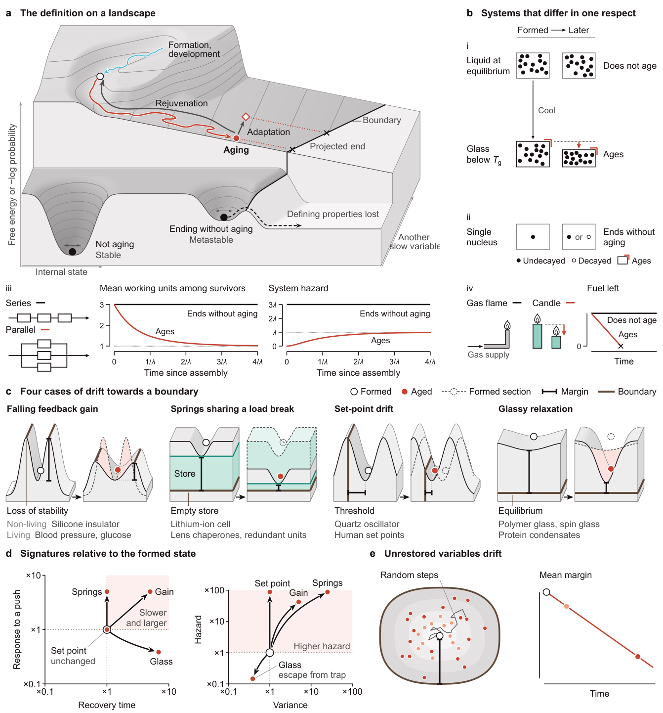
Figure 3.
The definition applied to organisms. a, Reserve over a life, on a landscape whose height is −log probability, with the slow variables along the life and the fast variables in depth. Reserve, drawn as the height of the boundary above the state, rises in development (light blue) from the start of life (small dot), peaks at the open circle and falls in aging (red). Dashed arrows mark jumps: a challenge; an injury, which carries the state forward along its course; rejuvenation (green), which carries it back from the present (red disc); and death, a small push across the lowered boundary. Solid blue arrows mark responses: the return after a challenge, and adaptation, which lowers the state into a dimple without moving the boundary. b, What aging clocks estimate, on a landscape over two slow variables whose rim (brown) is the boundary. Development (light blue) carries the state from the start of life (small dot) to peak reserve (open circle), and aging (red) carries it to the present (red disc). Ticks mark equal intervals of chronological time, which clocks trained on chronological age estimate. The reserve (I-bar), which clocks trained on mortality estimate, is drawn as the height of the boundary above the state, measured where the present drift, extended by the dotted red line, would reach the boundary (projected death). Pace clocks [101] estimate the speed of drift (thick red arrow), and causal clocks [102] separate the changes that carry the state towards the boundary (thin red arrow) from those that carry it away (gray arrow), shown enlarged in the circle, whose brown arc marks the boundary. c, Biological and omic ages. Above, biological age. An individual of chronological age t has biological age B if its reserve (red disc) equals the median reserve of the living members of a reference cohort (gray), read on its declining limb at age B, and B − t is the age gap. The median reaches the boundary only as the last members of the cohort die. Below, the state moves through a space of many variables, drawn as three omic layers in perspective (red course to the present state, red disc). Its projection onto each layer (dashed, by way of its shadows on the floor and the wall) is that layer’s reading, and the age at which the reference cohort has the same reading (ticks) is the omic age, so the proteomic, transcriptomic and epigenetic ages of one state differ. Biological age uses all variables of the state through its reserve (above). d, Two individuals with the same reserve (red disc), and so the same biological age, reach the boundary at different times if they drift at different speeds. e, A shorter-lived and a longer-lived species drawn at one scale, with ticks at one chronological interval and reserve against age below each. The shorter-lived species has a smaller and shallower region, a lower peak reserve and faster drift. f, Ways to extend life, grouped by what they change. Each cell shows a landscape above reserve against age, with the reference in gray and the change in green; the area that a boundary change adds to the living region is hatched and old boundaries are dashed. Discs mark the state at the moment of the change (gray, before; green, after), open circles mark peak reserve and crosses mark death where a course reaches the boundary; in a landscape a green cross marks only a crossing that the change moves. A higher peak is reached in a pit in the floor. A moved boundary moves out all around, and its landscape is drawn smaller so that the extended wall fits, whereas a reshaped boundary fills only the notch where the reference course ended. With fewer events, a life that would have ended in an event (dashed arrow) continues to the boundary. With slower drift, ticks at one interval of age lie closer together on the green course than on the gray. Rejuvenation returns the state along its course to an earlier point, replacement resets one drifted slow variable along a grid line, and adaptation lowers the state into a dimple that forms beneath it (solid arrow, a response), raising reserve while the drifted slow variables stay where they were. In each plot zero is the boundary of the reference landscape, so the gray arch is the same in every plot, and for a moved boundary the new boundary (solid) lies below zero and the green course continues down to it. Panels are schematics; effect sizes are illustrative and set to give similar gains in lifespan.
Figure 3.
The definition applied to organisms. a, Reserve over a life, on a landscape whose height is −log probability, with the slow variables along the life and the fast variables in depth. Reserve, drawn as the height of the boundary above the state, rises in development (light blue) from the start of life (small dot), peaks at the open circle and falls in aging (red). Dashed arrows mark jumps: a challenge; an injury, which carries the state forward along its course; rejuvenation (green), which carries it back from the present (red disc); and death, a small push across the lowered boundary. Solid blue arrows mark responses: the return after a challenge, and adaptation, which lowers the state into a dimple without moving the boundary. b, What aging clocks estimate, on a landscape over two slow variables whose rim (brown) is the boundary. Development (light blue) carries the state from the start of life (small dot) to peak reserve (open circle), and aging (red) carries it to the present (red disc). Ticks mark equal intervals of chronological time, which clocks trained on chronological age estimate. The reserve (I-bar), which clocks trained on mortality estimate, is drawn as the height of the boundary above the state, measured where the present drift, extended by the dotted red line, would reach the boundary (projected death). Pace clocks [101] estimate the speed of drift (thick red arrow), and causal clocks [102] separate the changes that carry the state towards the boundary (thin red arrow) from those that carry it away (gray arrow), shown enlarged in the circle, whose brown arc marks the boundary. c, Biological and omic ages. Above, biological age. An individual of chronological age t has biological age B if its reserve (red disc) equals the median reserve of the living members of a reference cohort (gray), read on its declining limb at age B, and B − t is the age gap. The median reaches the boundary only as the last members of the cohort die. Below, the state moves through a space of many variables, drawn as three omic layers in perspective (red course to the present state, red disc). Its projection onto each layer (dashed, by way of its shadows on the floor and the wall) is that layer’s reading, and the age at which the reference cohort has the same reading (ticks) is the omic age, so the proteomic, transcriptomic and epigenetic ages of one state differ. Biological age uses all variables of the state through its reserve (above). d, Two individuals with the same reserve (red disc), and so the same biological age, reach the boundary at different times if they drift at different speeds. e, A shorter-lived and a longer-lived species drawn at one scale, with ticks at one chronological interval and reserve against age below each. The shorter-lived species has a smaller and shallower region, a lower peak reserve and faster drift. f, Ways to extend life, grouped by what they change. Each cell shows a landscape above reserve against age, with the reference in gray and the change in green; the area that a boundary change adds to the living region is hatched and old boundaries are dashed. Discs mark the state at the moment of the change (gray, before; green, after), open circles mark peak reserve and crosses mark death where a course reaches the boundary; in a landscape a green cross marks only a crossing that the change moves. A higher peak is reached in a pit in the floor. A moved boundary moves out all around, and its landscape is drawn smaller so that the extended wall fits, whereas a reshaped boundary fills only the notch where the reference course ended. With fewer events, a life that would have ended in an event (dashed arrow) continues to the boundary. With slower drift, ticks at one interval of age lie closer together on the green course than on the gray. Rejuvenation returns the state along its course to an earlier point, replacement resets one drifted slow variable along a grid line, and adaptation lowers the state into a dimple that forms beneath it (solid arrow, a response), raising reserve while the drifted slow variables stay where they were. In each plot zero is the boundary of the reference landscape, so the gray arch is the same in every plot, and for a moved boundary the new boundary (solid) lies below zero and the green course continues down to it. Panels are schematics; effect sizes are illustrative and set to give similar gains in lifespan.
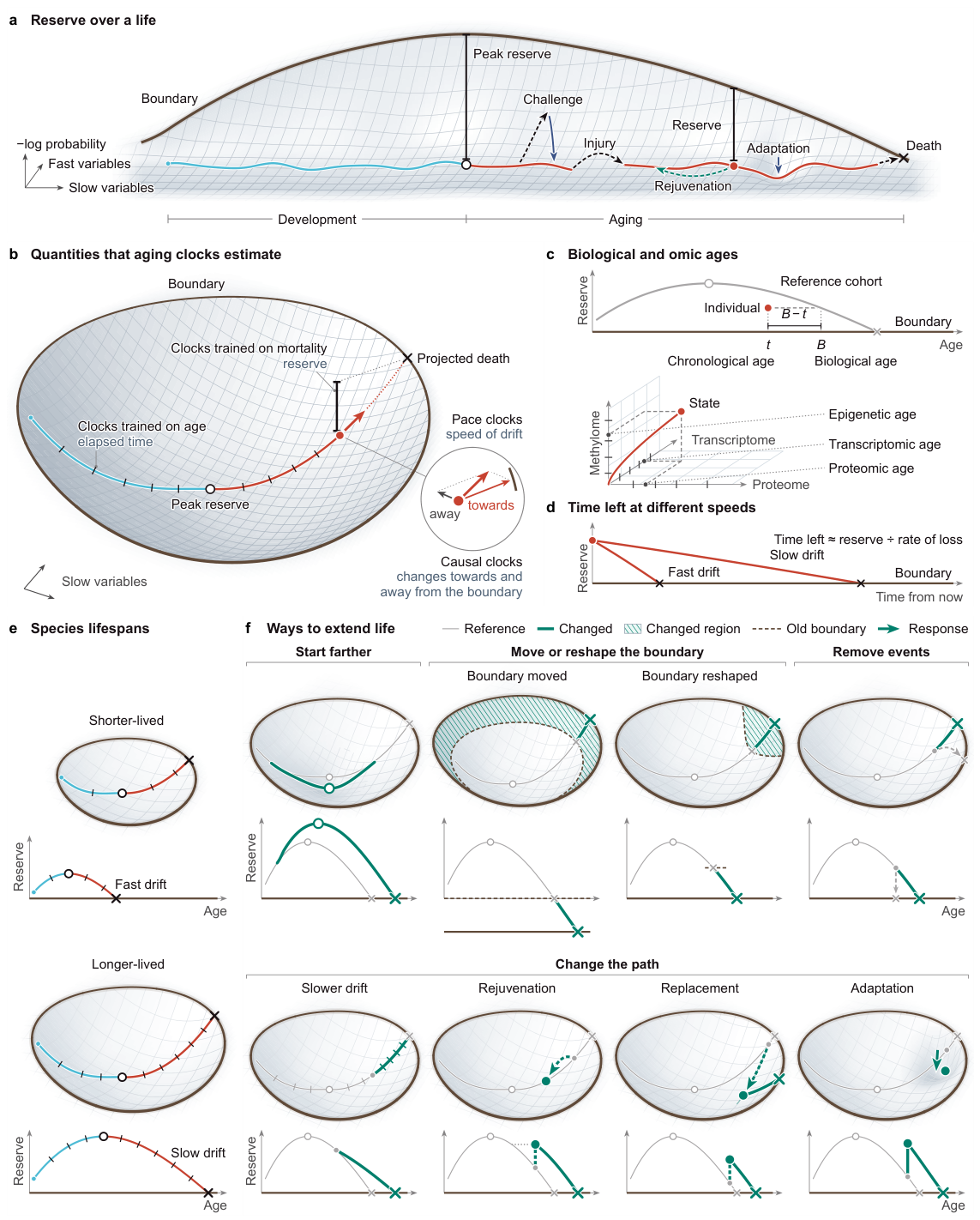
Disclaimer/Publisher’s Note: The statements, opinions and data contained in all publications are solely those of the individual author(s) and contributor(s) and not of MDPI and/or the editor(s). MDPI and/or the editor(s) disclaim responsibility for any injury to people or property resulting from any ideas, methods, instructions or products referred to in the content. |
© 2026 by the author. Licensee MDPI, Basel, Switzerland. This article is an open access article distributed under the terms and conditions of the Creative Commons Attribution (CC BY) license.
Copyright: This open access article is published under a Creative Commons CC BY 4.0 license, which permit the free download, distribution, and reuse, provided that the author and preprint are cited in any reuse.