

Submitted:
16 November 2026
Posted:
18 November 2026
You are already at the latest version
Abstract
Background: When small-sample intervals for a difference of two arithmetic means fail under skewness, they fail mostly on one side, given by the sign of the skewness balance . Bayesian intervals are increasingly proposed for small studies, including confirmatory ones. We asked whether Bayesian intervals inherit this direction, and whether modelling the skewness removes it. Methods: Two registered simulation studies. Study 1 computed the independence-Jeffreys (fiducial) and Jeffreys-rule normal-likelihood intervals on exactly the 655 cells 10,000 datasets of two earlier studies, regenerated from archived seeds, and tested six hypotheses on direction, inheritance, first-order equivalence, opposed skew, null behaviour and validity. Study 2 compares posterior intervals from lognormal, gamma, Weibull and skew-normal likelihoods (correctly and incorrectly specified), stacking, and informative shape priors with Welch, bootstrap-t and a beta-bootstrap-t in 156 settings of positive-valued populations. Results: Study 1: the recomputed Welch and Hsu results matched the archived results exactly in all 655 cells. Both Bayesian intervals failed on the side of sign in 97.1–99.3% of determinate cells and on the same side as Welch in every cell where both were determinate (456 of 456 and 457 of 457); for groups of at least 30 the slope of their imbalance on Welch’s was 0.967–1.003. The prior changed the size slightly, never the side. Study 2: with a correctly specified skewed likelihood and groups of at least 20, the imbalance was at most half of Welch’s with coverage within 951.5 percentage points in 29 of 34 cells (median ratio to Welch 0.08), at a median width 1.33 times Welch’s. Misspecified fits were directionally worse than Welch in 4 of 120 (gamma), 7 of 132 (Weibull), 23 of 120 (lognormal) and 47 of 144 (skew-normal) cells; for the lognormal and skew-normal fits this happened most often at the largest group sizes. Stacking was not worse than the normal model in 58 of 66 cells, below the registered 90%. The effect of a wrongly centred shape prior decreased from 10 to 50 per group in 20 of 24 combinations. The correct model and stacking had smaller imbalances than bootstrap-t and beta-bootstrap-t in most cells. Conclusions: Noninformative priors do not change the side on which normal-likelihood intervals fail. In the families studied, a skewed likelihood removed the directional failure when it was the correct family, but a wrong skewed model could fail more than Welch’s interval, and more so as the groups grew. Credible intervals proposed for one-sided decisions in small studies should be evaluated for their one-sided error under plausible alternative families, not only under the model that produced them.
Keywords:
Behrens–Fisher problem
; Bayesian credible interval
; fiducial interval
; Jeffreys prior
; skewness
; model misspecification
; stacking
; bootstrap-t
; directional error
; preregistration
1. Introduction
Comparing two groups by the difference of their arithmetic means, , is among the most common inferential tasks, and when the group variances may differ it is the Behrens–Fisher problem [1,2,3]. In two earlier preregistered studies we showed that when small-sample intervals for fail under skewness, they fail mostly on one side [4,5]. The side is predicted by the sign of the skewness balance
where and are the third central moment and the variance of group . is the standardised third cumulant of the difference in sample means; it appears in the two-sample Edgeworth expansions of Zhang and Wang [6] and, for one sample, in classical results on the studentised mean [7,8]. To first order the imbalance between the probability that the interval lies entirely below and the probability that it lies entirely above is
with and the standard normal density. The direction matters more than the total coverage suggests: many scientific and practical decisions are one-sided, so an interval with near-nominal total coverage can have a one-sided error well above the nominal 2.5% on the side that decides the claim [4]. In Paper 2 we showed that the allocation of a fixed sample between the groups moves this direction as predicts, but that no allocation removes it when the groups are skewed in opposite directions [5].
Bayesian intervals are increasingly proposed for small studies, including confirmatory ones. That raises two questions that, as far as we know, have not been tested directly. First, do Bayesian intervals under standard noninformative priors fail on the same side as Welch’s interval, and by how much? The normal-likelihood posterior for under the independence-Jeffreys prior is Fisher’s fiducial interval [2,9], and Hsu’s interval [10] is the inferential-model solution [11]; it would be surprising if they behaved differently, but surprise is not evidence, and the size of any difference is unknown. Second, and more importantly, does a model that represents the skewness remove the directional failure, and what happens when that model is wrong? Skewed likelihoods are the natural Bayesian answer for positive outcomes such as costs [12,13,14,15] and give asymmetric intervals for the arithmetic mean [16], but their one-sided error has not, to our knowledge, been studied.
We answered these questions with two preregistered studies. Study 1 [17] computes two normal-likelihood Bayesian intervals on exactly the datasets of Papers 1 and 2, so that every comparison with Welch is paired dataset by dataset. Study 2 [18] generates new positive-valued data and compares posterior intervals from correctly and incorrectly specified skewed likelihoods, stacking across models [19] and informative priors with the strongest frequentist asymmetric intervals, bootstrap-t and the beta-bootstrap-t [20]. We registered in advance that “Bayesian intervals are no better than bootstrap-t” and “worse under misspecification” are acceptable outcomes.
2. Methods
2.1. Registration and Reporting
Each study had a predeclared plan, frozen with a SHA-256 fingerprint and registered on Zenodo before any computation on study data [17,18]. Both plans were finalised after accuracy checks and pilots on separate, non-study random seeds; every change between the draft and the frozen plan is listed in the plan. Study 2’s confirmatory analysis script was frozen and fingerprinted with its plan. We follow the reporting recommendations of Morris et al. [21]. Paper 1, Paper 2 and pilot data are never pooled with each other or with the new data. There was one deviation from the Study 2 plan, a numerical one, reported in Section 3.2.
2.2. Study 1: Normal-Likelihood Intervals on the Datasets of Papers 1 and 2
Data. Study 1 introduces no new random data. It regenerates the 147 Paper 1 settings and the 316 oracle-allocation and 192 pilot-allocation runs of Paper 2, each with 10,000 datasets and , from their archived seeds and code [4,5]. All intervals studied are translation- and scale-equivariant, so loses nothing. As an identity check, the Welch and Hsu intervals were recomputed and required to match the archived Paper 1 counts and the archived Paper 2 dataset-level indicators exactly; any mismatch would have stopped the study.
Intervals. Each group has a normal likelihood with its own mean and variance, and the groups are independent a priori. With the difference in sample means, the posterior of is the distribution of
where and are independent Student-t variables, and the equal-tailed 95% interval is , with the 97.5% quantile of and . Under the independence-Jeffreys (reference) prior (interval J1, the Behrens–Fisher fiducial interval) and under the Jeffreys-rule prior (interval J2),
The quantile was computed by Newton’s method on
with , , and indexing the components with the larger and smaller weight, and Gauss–Legendre quadrature (512 nodes) after an endpoint transform that removes the singularity of heavy-tailed quantile functions. was tabulated on 2,001 points of for each pair of degrees of freedom and interpolated by monotone cubic interpolation of the normalised quantile. Before any study computation, the interpolation error was below (registered limit ), the quadrature agreed with adaptive integration to , and all six comparisons with -draw Monte Carlo quantiles were within Monte Carlo error. The Welch and Hsu intervals [3,10] were recomputed on the same datasets.
Performance measures. Coverage, , , and mean width, with the Monte Carlo standard error
An imbalance is determinate when . Dataset-level indicators allow paired contrasts with a paired bootstrap standard error.
Hypotheses (each for J1 and J2, and for Paper 1 and Paper 2 cells separately). S1, direction: in cells with , in at least 90% of determinate cells. S2, inheritance: where both the Bayesian and the Welch imbalance are determinate, their signs agree in at least 95% of cells. S3, first-order equivalence: for , the through-origin slope of the Bayesian on the Welch lies in [0.9, 1.1]. S4, opposed skew: in at least 95% of opposed-skew cells. S5, null cells : at most 5% with . S6, validity under normality (J1, fixed allocations): coverage at least in every cell, as the fiducial interval is reported to be conservative under normality [22].
Theory. S3 corresponds to a first-order statement for the class of symmetric intervals. If with and
then, under finite sixth moments and Cramér’s condition, has the same leading imbalance (2) as Welch’s interval. This covers Welch, Hsu, J1, J2 and normal-model posterior intervals whose prior influence is . It is not a new result: the one-sided term is even in and is Hall’s [7] for one sample and Zhang and Wang’s [6] for the Welch statistic, and a critical value that differs from by changes each tail only at order . We state it as a lemma; Study 1 provides the exact finite-sample answer on every dataset.
2.3. Study 2: Modelling the Skewness
Populations. Study 2 uses positive-valued populations, for which the arithmetic mean is often the quantity needed, as with costs [15]: lognormal (log-scale standard deviation 0.5 or 1.0), gamma (shape 0.5 or 2), Weibull (shape 0.8 or 1.5), a skew-normal shifted to be effectively positive [23], a two-component lognormal mixture that no candidate model fits, and a gamma with shape 50 as a near-null control. Thirteen group pairings (same family and shape; same family, different shapes; cross-family; control), six pairs of group sizes from (5, 5) to (50, 50) including (10, 40) and (40, 10), and , 0.5} give 156 settings. is computed exactly for each setting; it ranges from −1.31 to 2.47, and 25 settings have .
Intervals. All are computed on identical datasets within a setting:
- • B0: the J1 interval of Study 1; B1: the Bayesian bootstrap [24].
- • B2: each group fitted with its own correct model (lognormal, gamma, Weibull or skew-normal) under an objective prior; defined in the 12 pairings without the mixture.
- • B3: one model (lognormal, gamma, Weibull or skew-normal) fitted to both groups, in every setting; it is misspecified whenever the model is wrong for at least one group. The skew-normal is a common software default for skewed outcomes.
- • B4: stacking of the predictive distributions of the normal, lognormal, gamma and Weibull models [19], with weights from exact leave-one-out predictive densities.
- • B5a and B5b: B2 with the shape prior replaced by an informative normal prior on the log shape (standard deviation 0.25), centred on the true shape (B5a) or on the shape with half the true skewness (B5b).
- • F1: Welch; F2: bootstrap-t; F3: our two-sample extension of the beta-bootstrap-t [20].
Priors and computation. Lognormal: on the log scale, with exact conjugate posterior draws. Gamma and Weibull: Jeffreys priors, [9,25] and [26]. Skew-normal: flat in location, in scale and an approximation to the Jeffreys prior for the shape [27]. Posteriors of the arithmetic mean were computed on grids that follow the conditional posterior of the location given the shape (two-dimensional; three-dimensional and in two stages for the skew-normal), with automatic widening whenever more than of posterior mass reached a grid edge. Against much finer grids or exact draws, interval endpoints agreed to within 3% of the interval width at (5% for the lognormal grid against Monte Carlo reference draws, which carry most of that difference) and to within 1.7% for . Intervals are equal-tailed 95% intervals from 25,000 posterior draws (16,000 for B1; 15,999 resamples for F2 and F3). These sizes were set by a registered check: rerunning the intervals with independent random streams changed the below/above classification of fewer than 0.5% of datasets for every interval (largest 0.42%).
Hypotheses. T1: B0 fails on the side of in at least 90% of determinate eligible cells. T2 (primary bar): for groups of at least 20, a correct model at least halves Welch’s imbalance with coverage within percentage points in at least 80% of cells; a stricter and a looser bar are registered as sensitivity analyses. T3: misspecified fits are classified as directionally unsafe, neutral or improved relative to Welch, with no direction predicted. T4: stacking is never worse than B0 on direction in at least 90% of cells. T5: the effect of the wrong prior is larger at (10, 10) than at (50, 50) in at least 80% of combinations. T6: Bayesian intervals are compared with F2 and F3 without a predicted direction. T7: at most 5% of the 25 null settings flag an imbalance beyond 3 MCSE, for every interval.
Scale. Each setting has 10,000 datasets. Under a compute rule registered in advance, the posterior-draw intervals (B1–B5) are computed on the first 5,000 datasets of each setting and B0, F1, F2 and F3 on all 10,000; at 5,000 datasets the Monte Carlo standard error of is at most 0.32 percentage points when .
2.4. Implementation, Checks and AI Assistance
Simulations were written in Python (NumPy, SciPy). Before each main run, accuracy checks, logical checks and a pilot were run on separate seeds; the Study 2 pilot found two numerical problems (a Weibull overflow and an insufficiently accurate skew-normal grid), which were fixed before freezing. The research programme, the questions of this paper and the design choices of both studies are the author’s, building on Papers 1 and 2 [4,5]. The author used Claude (Anthropic), an AI assistant, as a research assistant: it drafted the plans from the author’s decisions, wrote the simulation and analysis code, ran the simulations in an isolated cloud computing environment and drafted figures and text. All design decisions were made or approved by the author, who registered both plans, reviewed every output, decided how results are reported and takes responsibility for the methods, interpretations, citations and final text. AI assistance did not constitute independent validation.
3. Results
3.1. Study 1: Noninformative Priors Inherit the Side of Failure
The recomputed Welch and Hsu intervals matched the archived Paper 1 counts and Paper 2 dataset-level indicators exactly in all 655 cells, so the Bayesian intervals were computed on identical datasets. All six hypotheses were supported for both priors and in both sets of cells (Table 1).
Across all cells where both imbalances were determinate, J1 failed on the same side as Welch in 456 of 456 and J2 in 457 of 457. The few direction disagreements in S1 were inherited rather than new: in Paper 2, J1 disagreed with in exactly the two cells where Welch did (a lognormal group against an exponential one, at total sizes 40 and 20), and in Paper 1 the disagreeing cells were the most extreme setting, with variance ratio 10, where Welch also disagreed. Figure 1 shows the paired imbalances: the Bayesian intervals lie on the line of equality, slightly below it for J1 and slightly above it for J2 in the cells with the largest imbalances.
The prior changed the size of the imbalance, not its side, and only at small (Table 2). J1 is slightly more conservative than Welch: its imbalance was about 15% smaller when the smaller group had 5 to 9 observations and about 2% smaller from 50 observations; the reduction was significant in the paired contrasts in 63 of 147 Paper 1 cells and 203 of 508 Paper 2 cells, at the cost of intervals about 2% wider. J2 was slightly worse than Welch: its imbalance was as large or larger, and its coverage was lower (Paper 1 median 93.87%, minimum 67.0%, against 94.70% median for Welch).
3.2. Study 2: Modelling the Skewness
The frozen analysis script ran unmodified on the complete main run of 156 settings. There was one deviation from the plan. In one of the 780,000 datasets analysed by the posterior-draw intervals (two gamma groups with shape 0.5, , ), the exact lognormal posterior draws of both group means exceeded the double-precision range on the same draw. Their difference was then undefined, the B3 lognormal interval was not finite, and the run stopped under the registered rule. With the author’s approval, the undefined draw (1 of 25,000) was left out of the quantiles in rows that contained one; every other row was computed exactly as registered, which was confirmed bit for bit against completed settings. Both versions of the code and the deviation record are archived. Table 3 summarises the confirmatory results.
Normal model (T1). The fiducial interval B0 failed on the side of in all 103 determinate eligible settings, which extends the Study 1 result to Weibull, skew-normal and mixture populations (Figure 2, top left).
Correct model (T2). With each group fitted by its own correct family, the imbalance in groups of at least 20 was a small fraction of Welch’s (median ratio 0.08), and coverage ranged from 94.28% to 96.18%. In all five settings that missed the primary bar, coverage was within the bar and only the ratio failed; Welch’s own imbalance there was small, 0.49 to 2.26 percentage points. The remaining imbalance had no consistent direction: where it was determinate and , its sign agreed with in 23 of 42 settings (Figure 2, bottom left). At (5, 5), where no criterion was registered, B2 had a smaller imbalance than Welch in 15 of 24 settings, with coverage from 93.3% to 98.4%.
Misspecification (T3). When one model was fitted to both groups and was wrong for at least one of them, the risk depended on the model (Table 3, Figure 3). Gamma and Weibull fits improved on Welch in most settings and were worse in 4 of 120 and 7 of 132. Lognormal and skew-normal fits were worse in 23 of 120 and 47 of 144. For these two models the unsafe settings were concentrated at the larger group sizes: at (50, 50), 10 of 20 lognormal and 13 of 24 skew-normal settings were unsafe, against none of either at (5, 5). This pattern by size is descriptive; T3 registered no direction. The largest failure was the lognormal model fitted to gamma (shape 0.5) vs gamma (shape 2) at (50, 50), : coverage 36.3%, with and .
Stacking (T4). Stacking over the normal, lognormal, gamma and Weibull models reduced the imbalance in most settings: the median was 0.3 to 1.2 percentage points by group size, against 1.4 to 5.0 for B0. It was significantly worse than B0 in 8 of 66 settings, so T4 was not supported. Three of these were lognormal vs mixture, the pairing that no candidate model fits, where B4 coverage was 88.9% to 91.2%; two were lognormal vs gamma (shape 2) at , and three were same-family settings at (5, 5) with .
Informative priors (T5). A shape prior centred on the correct value (B5a) gave the smallest imbalances of all intervals, with coverage of at least 94.44% (Table 5). A prior centred on half the true skewness (B5b) shifted the imbalance by less at (50, 50) than at (10, 10) in 20 of 24 combinations. In the four exceptions the shift grew: lognormal vs lognormal , (0.06 to 0.18 percentage points); skew-normal vs lognormal , (0.42 to 1.76 percentage points); skew-normal vs skew-normal, (0.02 to 0.64 percentage points); Weibull (shape 0.8) vs Weibull (shape 0.8), (0.36 to 0.76 percentage points).
Benchmarks (T6). The correct model and stacking had significantly smaller imbalances than both bootstrap intervals in most settings and significantly larger ones in at most 7 (Table 4). The bootstrap intervals reduced the imbalance relative to Welch but still failed on the side of : in 101 of 102 (bootstrap-t) and 101 of 102 (beta-bootstrap-t) determinate settings with (Figure 2). Stacking did so in 52 of 57.
Null control (T7). No interval flagged more than 1 of the 25 settings with . The flagged setting was the same for the five intervals that had one (the misspecified lognormal, skew-normal and Weibull fits and both bootstrap intervals): gamma (shape 0.5) vs gamma (shape 2) at (40, 10), , where only because the two skewness terms cancel, so that it is not a comparison of identical populations.
Coverage and width (exploratory). Table 5 summarises all intervals. The gains of the correct model and of stacking came with wider intervals, a median 1.33 and 1.46 times Welch’s. The lognormal fit was very wide (median 3.16 times) and had the lowest minimum coverage. The Bayesian bootstrap under-covered in most settings (median 89.22%, minimum 73.90%).

Table 5.
Study 2, all intervals across the 156 settings (B2, B5a and B5b: 144 settings). Exploratory; no criterion. and width ratios are medians over settings.
Table 5.
Study 2, all intervals across the 156 settings (B2, B5a and B5b: 144 settings). Exploratory; no criterion. and width ratios are medians over settings.
| Interval | Median coverage (%) | Minimum coverage (%) | Median $L - U$ (pp) | Median width / Welch |
|---|---|---|---|---|
| B0 fiducial (normal model) | 95.25 | 85.15 | 2.56 | 1.03 |
| B1 Bayesian bootstrap | 89.22 | 73.90 | 2.85 | 0.85 |
| B2 correct model | 95.08 | 93.26 | 0.46 | 1.33 |
| B3 lognormal | 95.51 | 36.26 | 0.70 | 3.16 |
| B3 gamma | 93.38 | 82.36 | 0.73 | 1.04 |
| B3 Weibull | 94.03 | 83.22 | 0.74 | 1.11 |
| B3 skew-normal | 92.17 | 52.22 | 3.07 | 0.98 |
| B4 stacking | 94.71 | 86.82 | 0.49 | 1.46 |
| B5a informative prior, correct centre | 95.56 | 94.44 | 0.32 | 1.12 |
| B5b informative prior, half the skewness | 89.64 | 72.88 | 1.65 | 0.88 |
| F1 Welch | 94.72 | 84.76 | 2.98 | 1.00 |
| F2 bootstrap-t | 93.47 | 86.79 | 2.21 | 1.08 |
| F3 beta-bootstrap-t | 93.69 | 86.19 | 2.33 | 1.04 |
4. Discussion
4.1. Study 1: The Prior Does Not Change the Side
On the same datasets, the two standard noninformative-prior Bayesian intervals failed on the same side as Welch’s interval in every cell where the comparison was informative, with the same first-order size. This is what the lemma predicts: all of these intervals are symmetric about the difference in sample means, , and differ only in , which shifts the two tails equally to the order that matters. The prior therefore acts on total coverage, not on direction. The fiducial interval’s heavier tails make it slightly more conservative and slightly less unbalanced at small , consistent with its reported conservativeness under normality [22], which S6 confirmed in every normal cell; the Jeffreys-rule prior, which uses rather than degrees of freedom, makes the interval shorter and its failures more frequent. Neither changes which side fails. For practice, choosing a noninformative prior is not a remedy for directional failure; the direction comes from the symmetric normal-likelihood interval, whatever its justification, fiducial [2], Bayesian [9] or inferential-model [11].
4.2. Does Modelling the Skewness Help?
Study 1 located the direction in the symmetric normal-likelihood interval; Study 2 asked whether an interval that is not symmetric removes it. When the likelihood was the correct family, it did, in the settings studied: the imbalance in groups of at least 20 was a small fraction of Welch’s, coverage stayed close to 95%, and the residual imbalance no longer had the sign of . Unlike the intervals of Study 1, a posterior interval from a skewed likelihood is not symmetric about the difference in sample means, so it can follow the skewness of the sampling distribution; a symmetric interval cannot. The price was width: about a third more than Welch’s interval at the median.
The repair depended on the model, and a wrong model could make the directional failure worse. Under misspecification, the posterior concentrates near the parameter value whose model is closest in Kullback–Leibler divergence to the true distribution [28,29]. The posterior of the arithmetic mean then centres on the mean of that closest model, which in general differs from the true mean. As grows the interval narrows around this value, so a fixed bias becomes a growing one-sided error; that is consistent with the concentration of unsafe lognormal and skew-normal fits at the largest sizes (Figure 3). The gamma and Weibull fits were rarely unsafe in our pairings, which says that their closest-model means were near the true means for these populations, not that they are safe in general. In the cost-data literature the estimated mean has likewise been found to depend on the distribution assumed [13,14]; our results add that, in the settings studied, the consequence for the interval has a direction, and that for the lognormal and skew-normal fits it grew rather than diminished with sample size.
Exploratory analysis (post hoc, not registered). Which mean the closest model has depends on the family. For an exponential family whose sufficient statistics include itself, the closest member matches exactly, whatever the true distribution [30]; the gamma (sufficient statistics and ) has this property, the lognormal ( and ) does not. To see whether this explains T3, we computed the pseudo-true mean of each fitted family under each population of Study 2 (maximum likelihood on 400,000 draws per population, separate seed). For a gamma population with shape 0.5 and mean 1, the closest lognormal has mean 3.26, the closest skew-normal 1.38, the closest gamma 1.00 and the closest Weibull 1.03; for a Weibull population with shape 0.8 the lognormal gives 1.56, and for a lognormal population with the skew-normal gives 1.33. In every population the gamma fit reproduced the true mean, as this property requires, and the Weibull fit was within 3% of it. Standardising the resulting bias in by the standard error of , the misspecified settings with |bias| < 0.1 standard errors were unsafe in 23 of 369, and those with standard error in 28 of 44. Because the standardised bias grows like , this would account for the growth of misspecification failures with . It also suggests choosing a likelihood for the arithmetic mean by this property rather than by fit, in line with the preference for gamma-type models over log models for mean costs [31]. The analysis was suggested by the results it explains and is therefore hypothesis-generating; it does not account for the failures that remain at small bias, which point to a mismatch in spread or shape.
Stacking reduced the imbalance in most settings but was not reliably better than the normal model (T4). Its weights maximise leave-one-out predictive performance of the whole density [19], whereas the arithmetic mean depends heavily on the upper tail, which a few observations cannot identify. Where no candidate fits, as with the mixture, a model can win on predictive density and still misstate the mean. Informative priors behaved as the argument predicts in most combinations: a prior centred on half the true skewness mattered less at 50 than at 10 per group in 20 of 24, and a correctly centred prior was the best interval of all, an oracle that is not available in practice.
The bootstrap-t is second-order accurate for a smooth function of means [7,8], yet at these sizes it still failed on the side of in almost every determinate setting, with a smaller imbalance than Welch’s. Our two-sample beta-bootstrap-t behaved similarly. Against both, the correct model and stacking had smaller imbalances in most settings. We had registered “no better than bootstrap-t” and “worse under misspecification” as acceptable outcomes; the second occurred for the lognormal and skew-normal fits, the first did not occur for the correct model or for stacking.
4.3. Implications for practice
For a small study whose decision is one-sided, the side on which an interval for fails matters as much as its total coverage [4]. Three implications follow, each limited to the families we studied. First, replacing Welch’s interval with a normal-model Bayesian interval under a noninformative prior does not change the side of failure. Second, a skewed likelihood can remove the directional failure, but only if its family is close to the truth; the stacking results suggest that groups of this size do not reliably identify the family. Third, when a skewed model is used, its one-sided error should be examined under plausible alternative families, for example by refitting under each, and an analysis whose conclusion depends on the family should be reported as such.
More generally, a credible interval used as a confidence interval is justified only by its repeated-sampling coverage, and our results suggest that this coverage should be evaluated one side at a time, under the populations that are plausible for the outcome and not only under the model that produced the interval. We make no claim about Bayesian methods in general, about informative priors on the effect itself or about decision-theoretic uses of posterior distributions.
4.4. Limitations
Study 1 is limited to normal-likelihood intervals with two standard priors and inherits the populations, sizes and 95% level of Papers 1 and 2; it uses , which loses nothing only because all intervals compared are equivariant. Informative priors on the means, hierarchical models and adjusted analyses were not studied. As in Papers 1 and 2, no uniform guarantee is possible without restricting the class of populations [32], so all statements are conditional on the families studied.
Study 2 used six positive-valued families, one mixture, six pairs of group sizes, two values of and a 95% level; other families, especially heavier-tailed ones, may behave differently. The correct-model interval B2 is an oracle. The objective priors for each family are one reasonable choice among several, and the stacking candidates did not include the skew-normal. Posteriors of the gamma, Weibull and skew-normal means were computed on grids whose endpoint accuracy was checked in advance (within 3% of the interval width at , 1.7% for ), and the posterior-draw intervals were evaluated on 5,000 datasets per setting under the registered compute rule, so that their Monte Carlo standard error of was up to 0.32 percentage points when . The one deviation from the plan concerned a single draw in a single dataset. Unsafe, neutral and improved were defined relative to Welch’s interval; a different reference would give different shares.
5. Conclusions
Normal-likelihood Bayesian intervals under the standard noninformative priors failed on the same side as Welch’s interval, with the same first-order size; the prior changed total coverage, not the side. Modelling the skewness removed the directional failure only when the model was right: a correct skewed likelihood essentially removed the imbalance, whereas a wrong one could leave a larger imbalance than Welch’s, increasingly with sample size, and stacking did not reliably protect against this. In the settings studied, a Bayesian interval for a difference in means was a remedy for directional failure only to the extent that its family was right, and its one-sided error should be evaluated under the families that could have produced the data.
Funding
No funding was received for this study.
Data and code availability
The Study 1 plan, code, quantile tables and pilot are archived at doi:10.5281/zenodo.23988719; the Study 2 plan, code, frozen analysis, validations and pilot at doi:10.5281/zenodo.23999725 and doi:10.5281/zenodo.24000485. Main-run outputs, the frozen-analysis output and the verification notebooks for both studies are archived at doi:10.5281/zenodo.24280940. The datasets of Study 1 are regenerated from the archives of Papers 1 and 2 [4,5].
Competing interests
The author declares no competing interests.
Ethics
The study uses simulated data and involves no human participants or personal data
Acknowledgements
None.
Contributors and guarantor
J.G.L.V. conceived the research programme and the questions of this paper; chose the Bayesian framing, the comparison of noninformative priors on the earlier datasets, and the design of Study 2 (populations, models, the misspecification, stacking and prior-sensitivity arms, the benchmarks and the thresholds, including the registered sensitivity bars); approved the hypotheses and the theory statement; registered both plans and deposited all archives; reviewed the outputs and decided their interpretation and reporting; and is the guarantor who accepts responsibility for the integrity of the work and the accuracy of its reporting. AI assistance is disclosed in Section 2.4.
References
- Behrens, W.-V. Ein Beitrag zur Fehlerberechnung bei wenigen Beobachtungen. Landwirtsch. Jahrbücher 1929, 68, 807–837. [Google Scholar]
- Fisher, R. A. The fiducial argument in statistical inference. Ann. Eugen. 1935, 6(no. 4), 391–398. [Google Scholar] [CrossRef]
- Welch, B. L. The generalization of “Student’s” problem when several different population variances are involved. Biometrika 1947, 34(no. 1–2), 28–35. [Google Scholar] [CrossRef] [PubMed]
- Verheyden, J. G. L. Which way do small-sample confidence intervals for a difference of means fail? Coverage, directional error and the signed skewness balance, manuscript (2026). Data Code Zenodo. [CrossRef]
- Verheyden, J. G. L. Allocating a fixed sample between two groups: variance-optimal designs and the direction of small-sample confidence-interval failure, manuscript (2026); registered plan: Zenodo. [CrossRef]
- Zhang, H.; Wang, H. Transformation tests and their asymptotic power in two-sample comparisons. J. Nonparametr. Stat. 2021, 33(no. 3–4), 482–516. [Google Scholar] [CrossRef]
- Hall, P. Theoretical comparison of bootstrap confidence intervals. Ann. Stat. 1988, 16(no. 3), 927–953. [Google Scholar] [CrossRef]
- P. Hall, The Bootstrap and Edgeworth Expansion, Springer Series in Statistics, Springer, New York, 1992.
- H. Jeffreys, Theory of Probability, 3rd ed., Oxford University Press, Oxford, 1961.
- Hsu, P. L. Contributions to the theory of “Student’s” t-test as applied to the problem of two samples. Stat. Res. Mem. 1938, 2, 1–24. [Google Scholar]
- Wang, X.; Liu, C. Revisiting the Behrens–Fisher problem: Validity-first optimality. arXiv 2026, arXiv:2606.07847. [Google Scholar]
- O’Hagan, A.; Stevens, J. W. Assessing and comparing costs: how robust are the bootstrap and methods based on asymptotic normality? Health Econ. 2003, 12(no. 1), 33–49. [Google Scholar] [CrossRef] [PubMed]
- Nixon, R. M.; Thompson, S. G. Parametric modelling of cost data in medical studies. Stat. Med. 2004, 23(no. 8), 1311–1331. [Google Scholar] [CrossRef] [PubMed]
- Briggs, A.; Nixon, R.; Dixon, S.; Thompson, S. Parametric modelling of cost data: some simulation evidence. Health Econ. 2005, 14(no. 4), 421–428. [Google Scholar] [CrossRef] [PubMed]
- Thompson, S. G.; Barber, J. A. How should cost data in pragmatic randomised trials be analysed? BMJ 2000, 320(no. 7243), 1197–1200. [Google Scholar] [CrossRef] [PubMed]
- Harvey, J.; van der Merwe, A. J. Bayesian confidence intervals for means and variances of lognormal and bivariate lognormal distributions. J. Stat. Plan. Inference 2012, 142(no. 6), 1294–1309. [Google Scholar] [CrossRef]
- Verheyden, J. G. L. Paper 3, Study 1 — predeclared plan v1.0: do normal-likelihood Bayesian intervals fail on the same side as Welch’s? (Behrens–Fisher programme). Zenodo 2026. [Google Scholar] [CrossRef]
- Verheyden, J. G. L. Paper 3, Study 2 — predeclared plan v1.0: does modelling the skewness remove the directional failure of small-sample intervals for a difference in means? (Behrens–Fisher programme), Zenodo (2026), registration package. [CrossRef]
- Yao, Y.; Vehtari, A.; Simpson, D.; Gelman, A. Using stacking to average Bayesian predictive distributions. Bayesian Anal. 2018, 13(no. 3), 917–1007. [Google Scholar] [CrossRef]
- Owen, A.B. Better bootstrap t confidence intervals for the mean. arXiv 2025, arXiv:2508.10083. [Google Scholar]
- Morris, T. P.; White, I. R.; Crowther, M. J. Using simulation studies to evaluate statistical methods. Stat. Med. 2019, 38(no. 11), 2074–2102. [Google Scholar] [CrossRef] [PubMed]
- Robinson, G. K. Properties of Student’s t and of the Behrens–Fisher solution to the two means problem. Ann. Stat. correction. 1976, 4(no. 5 10 (1982), no. 1), 963–971 321. [Google Scholar] [CrossRef]
- Azzalini, A. A class of distributions which includes the normal ones. Scand. J. Stat. 1985, 12(no. 2), 171–178. [Google Scholar]
- Rubin, D. B. The Bayesian bootstrap. Ann. Stat. 1981, 9(no. 1), 130–134. [Google Scholar] [CrossRef]
- Moala, F. A.; Ramos, P. L.; Achcar, J. A. Bayesian inference for two-parameter gamma distribution assuming different noninformative priors. Rev. Colomb. Estad. 2013, 36(no. 2), 321–338. [Google Scholar]
- Sun, D. A note on noninformative priors for Weibull distributions. J. Stat. Plan. Inference 1997, 61(no. 2), 319–338. [Google Scholar] [CrossRef]
- Bayes, C. L.; Branco, M. D. Bayesian inference for the skewness parameter of the scalar skew-normal distribution. Braz. J. Probab. Stat. 2007, 21(no. 2), 141–163. [Google Scholar]
- Berk, R. H. Limiting behavior of posterior distributions when the model is incorrect. Ann. Math. Stat. 1966, 37(no. 1), 51–58. [Google Scholar] [CrossRef]
- Kleijn, B. J. K.; van der Vaart, A. W. The Bernstein–Von-Mises theorem under misspecification. Electron. J. Stat. 2012, 6, 354–381. [Google Scholar] [CrossRef]
- Gourieroux, C.; Monfort, A.; Trognon, A. Pseudo maximum likelihood methods: theory. Econometrica 1984, 52(no. 3), 681–700. [Google Scholar] [CrossRef] [PubMed]
- Manning, W. G.; Mullahy, J. Estimating log models: to transform or not to transform? J. Health Econ. 2001, 20(no. 4), 461–494. [Google Scholar] [CrossRef] [PubMed]
- Bahadur, R. R.; Savage, L. J. The nonexistence of certain statistical procedures in nonparametric problems. Ann. Math. Stat. 1956, 27(no. 4), 1115–1122. [Google Scholar] [CrossRef]
Figure 1.
Directional imbalance of the Bayesian intervals against that of Welch’s interval on identical datasets (each point one cell of 10,000 datasets; circles, Paper 1 cells; triangles, Paper 2 cells). The diagonal is the line of equality.
Figure 1.
Directional imbalance of the Bayesian intervals against that of Welch’s interval on identical datasets (each point one cell of 10,000 datasets; circles, Paper 1 cells; triangles, Paper 2 cells). The diagonal is the line of equality.
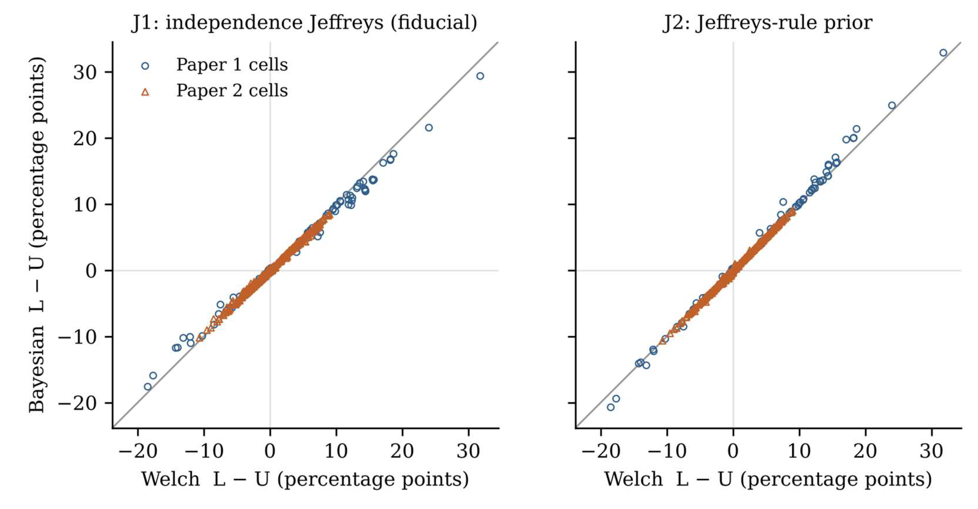
Figure 2.
Study 2: directional imbalance against the skewness balance for four intervals (each point one setting; B2 is defined in the 144 settings without the mixture). The grey line is the first-order law (2). The normal-model interval B0 and the bootstrap-t follow the sign of ; the correct skewed model does not; stacking lies between them.
Figure 2.
Study 2: directional imbalance against the skewness balance for four intervals (each point one setting; B2 is defined in the 144 settings without the mixture). The grey line is the first-order law (2). The normal-model interval B0 and the bootstrap-t follow the sign of ; the correct skewed model does not; stacking lies between them.
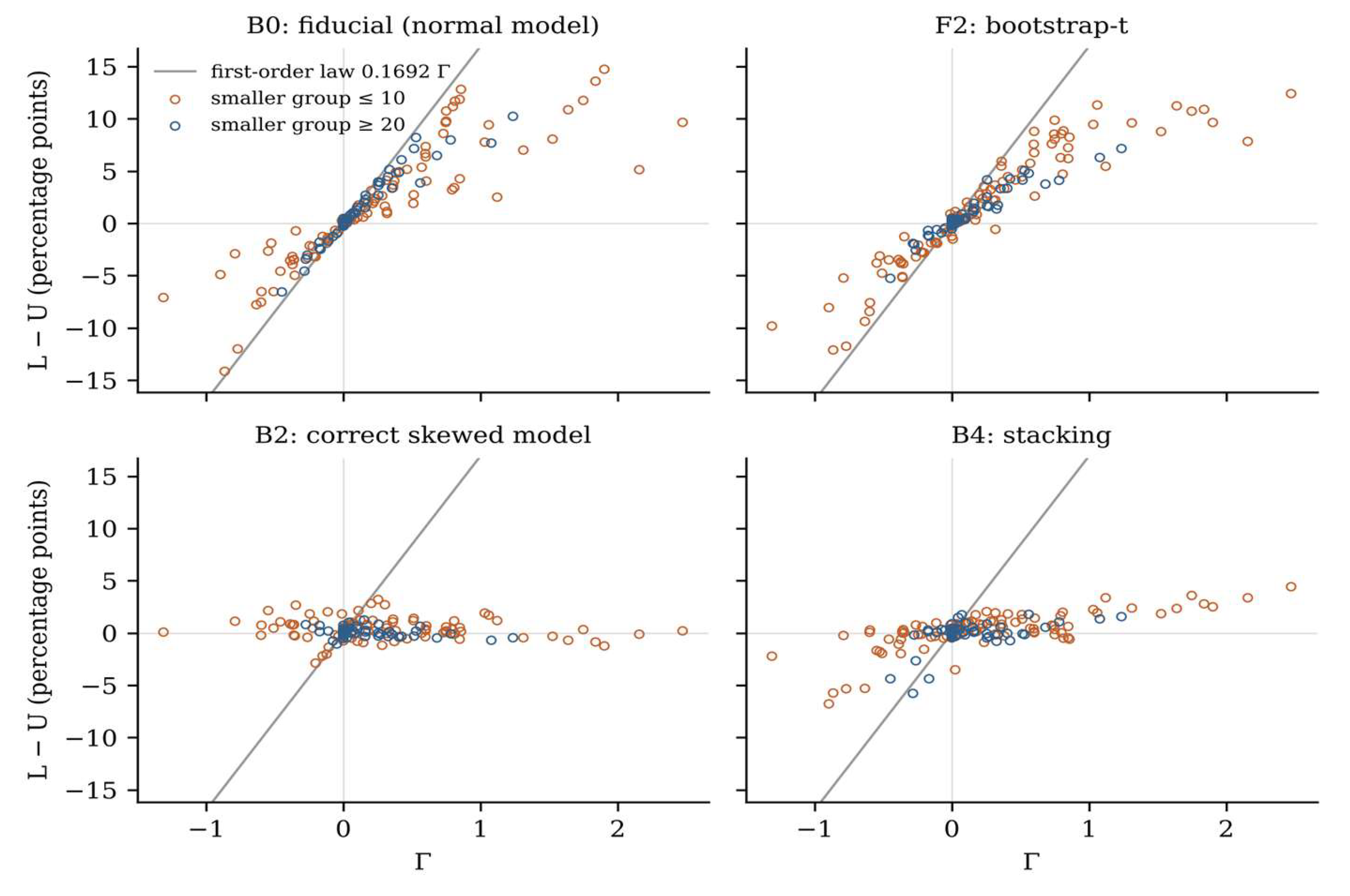
Figure 3.
Study 2: percentage of misspecified settings in which the fitted model was directionally worse than Welch’s interval (paired ), by fitted model and group sizes.
Figure 3.
Study 2: percentage of misspecified settings in which the fitted model was directionally worse than Welch’s interval (paired ), by fitted model and group sizes.
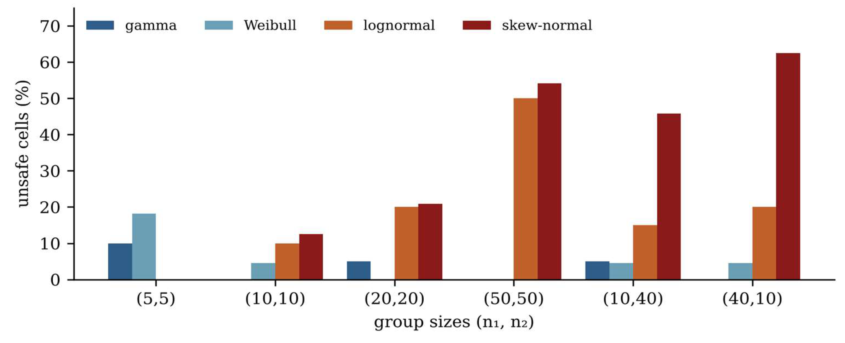
Table 1.
Study 1 confirmatory hypotheses. Paper 1 cells and Paper 2 cells are analysed separately; J1, independence-Jeffreys (fiducial) interval; J2, Jeffreys-rule interval. Every hypothesis met its registered criterion.
Table 1.
Study 1 confirmatory hypotheses. Paper 1 cells and Paper 2 cells are analysed separately; J1, independence-Jeffreys (fiducial) interval; J2, Jeffreys-rule interval. Every hypothesis met its registered criterion.
| Hypothesis | Paper 1, J1 | Paper 1, J2 | Paper 2, J1 | Paper 2, J2 |
|---|---|---|---|---|
| S1 direction: | 66/67 (98.5%) | 66/68 (97.1%) | 147/149 (98.7%) | 148/149 (99.3%) |
| S1 sensitivity (indeterminate = disagreement) | 95.7% | 95.7% | 96.1% | 96.7% |
| S2 same sign as Welch | 68/68 | 70/70 | 388/388 | 387/387 |
| S3 slope on Welch, | 0.975 | 1.003 | 0.967 | 0.999 |
| S3 slope, (no criterion) | 0.894 | 1.056 | 0.897 | 1.020 |
| S4 opposed skew: | 21/21 | 21/21 | 65/65 | 65/65 |
| S5 null cells flagged | 0/78 | 0/78 | 1/35 | 1/35 |
| S6 J1 coverage (normal data) | 21/21 (min 94.66%) | — | 25/25 (min 94.72%) | — |
Table 2.
Median ratio of the Bayesian to the Welch imbalance, , by the size of the smaller group (fixed-allocation cells with percentage points; Paper 1 and Paper 2 cells together, descriptive).
Table 2.
Median ratio of the Bayesian to the Welch imbalance, , by the size of the smaller group (fixed-allocation cells with percentage points; Paper 1 and Paper 2 cells together, descriptive).
| Smaller group, | Cells | J1 | J2 |
|---|---|---|---|
| 5–9 | 69 | 0.85 | 1.06 |
| 10–19 | 55 | 0.91 | 1.02 |
| 20–49 | 106 | 0.96 | 1.00 |
| 69 | 0.98 | 1.00 |
Table 3.
Study 2 confirmatory hypotheses. Cells are settings of 10,000 datasets (5,000 for the posterior-draw intervals); pp, percentage points; MCSE, Monte Carlo standard error. Only the primary T2 bar decides T2.
Table 3.
Study 2 confirmatory hypotheses. Cells are settings of 10,000 datasets (5,000 for the posterior-draw intervals); pp, percentage points; MCSE, Monte Carlo standard error. Only the primary T2 bar decides T2.
| Hypothesis | Cells | Holds | Criterion | Verdict |
|---|---|---|---|---|
| T1 B0 fails on the side of | 103 determinate of 103 eligible | 103 (100.0%) | supported | |
| T2 correct model: $L - U$ ≤ ½ Welch’s, coverage pp, (primary) | 34 | 29 (85.3%) | supported | |
| T2 sensitivity, stricter: ⅓ Welch’s, pp | 34 | 26 (76.5%) | not met | |
| T2 sensitivity, looser: significantly below Welch, pp | 34 | 29 (85.3%) | met | |
| T3 misspecified fits worse than Welch (unsafe): gamma, Weibull, lognormal, skew-normal | 120, 132, 120, 144 | 4, 7, 23, 47 | estimation | — |
| T4 stacking not worse than B0 on direction | 66 | 58 (87.9%) | not supported | |
| T5 wrong-prior effect larger at (10, 10) than at (50, 50) | 24 | 20 (83.3%) | supported | |
| T6 B2 and B4 against bootstrap-t and beta-bootstrap-t | Table 4 | — | none | — |
| T7 null settings with , each of 13 intervals | 25 | at most 1 | supported |
Table 4.
Study 2, T6: paired contrasts on the datasets both intervals share. Smaller and larger count settings with .
Table 4.
Study 2, T6: paired contrasts on the datasets both intervals share. Smaller and larger count settings with .
| Contrast | Settings | Bayesian smaller | Bayesian larger | Median (pp) |
|---|---|---|---|---|
| B2 vs bootstrap-t (F2) | 144 | 81 | 7 | −1.13 |
| B2 vs beta-bootstrap-t (F3) | 144 | 84 | 4 | −1.31 |
| B4 vs bootstrap-t (F2) | 156 | 98 | 5 | −1.42 |
| B4 vs beta-bootstrap-t (F3) | 156 | 100 | 5 | −1.48 |
Disclaimer/Publisher’s Note: The statements, opinions and data contained in all publications are solely those of the individual author(s) and contributor(s) and not of MDPI and/or the editor(s). MDPI and/or the editor(s) disclaim responsibility for any injury to people or property resulting from any ideas, methods, instructions or products referred to in the content. |
© 2026 by the authors. Licensee MDPI, Basel, Switzerland. This article is an open access article distributed under the terms and conditions of the Creative Commons Attribution (CC BY) license (http://creativecommons.org/licenses/by/4.0/).
Copyright: This open access article is published under a Creative Commons CC BY 4.0 license, which permit the free download, distribution, and reuse, provided that the author and preprint are cited in any reuse.