

Submitted:
16 November 2026
Posted:
17 November 2026
You are already at the latest version
Abstract
Neural surrogates of structures with fractional viscoelastic damping must carry the memory of the Caputo derivative and, over long horizons, must not create energy; penalty-based training guarantees neither. We propose TT-fpHNN, a port-Hamiltonian network in which the diffusive representation of the Caputo derivative with positive quadrature weights yields a finite port-Hamiltonian system for any number of memory nodes. Tail corrections with explicit bounds reduce the kernel error of a 24-node rule from 6.4% to 0.09%, a discrete-gradient integrator keeps the energy balance exact, and the learned operators are positive semidefinite tensor-train factors. On synthetic trusses, structured rollouts kept a per-step balance residual below \(10^{-12}\), whereas a sum-of-exponentials scheme of equal memory and accuracy accumulated a 1.7% energy imbalance. On 450 degrees of freedom, the rank-8 model reproduced 200 periods with 0.66% error and 11,106 parameters; an unconstrained model diverged, a model without memory reached 3.4%, and a regularised dense model needed 36.5 times more parameters. On 2160 degrees of freedom the model stayed passive over 10,000 steps with 3.3% error. Rank 16 over-fitted to a nearly singular stiffness. The fractional order was recovered within \(\pm0.05\) at 1% noise with two-decade excitation and biased at 5%. Single-precision materialisation at condition number \(7.7\times10^{7}\) destroyed definiteness.
Keywords:
port-Hamiltonian neural networks
; fractional viscoelasticity
; diffusive representation
; Caputo derivative
; tensor-train
; discrete gradient
; passivity
; digital twin
; structural dynamics
; identifiability
1. Introduction
A structural digital twin that runs alongside a monitoring campaign of six months ( s) with a time step of 1 to 5 ms integrates between and steps. Two properties of the surrogate model then decide whether its output can be used for damage or remaining-life estimates. The first is energetic consistency: if the model creates even a small amount of spurious energy per step, the cumulative balance loses physical meaning long before the campaign ends. The second is the cost of memory. Viscoelastic dampers, elastomeric bearings and polymer-modified members are described with fractional derivatives [1,2,3], and the Caputo derivative of order depends on the whole displacement history. A direct discretisation such as the L1 scheme [4] stores N past states and costs per step; at and degrees of freedom (DOF) the stored history alone would occupy about in double precision. Fast algorithms remove this growth: convolution quadrature with oblivious evaluation [5,6] and sum-of-exponentials approximations of the Caputo kernel [7] need a number of auxiliary states that is fixed or grows logarithmically with N. They bound the cost of memory, but they are numerical schemes for a known equation and carry no statement about the energy of a learned model.
Most neural surrogates used today in structural dynamics address neither property. Physics-informed neural networks (PINNs) impose the equation of motion as a penalty in the loss [8,9]; applications cover Bouc–Wen hysteresis [10,11], nonlinear system identification [12,13], damage in reinforced concrete piers [14] and fractional problems through fPINNs [15] and their descendants [16,17]. A penalty constrains the model only at collocation points and gives no guarantee during a long rollout. Digital twins built on graph networks or neural operators [18,19,20] share this limitation.
Structure-preserving learning takes a different route: the geometry of mechanics is built into the architecture. Hamiltonian and Lagrangian neural networks [21,22] conserve energy by construction; dissipative and port-Hamiltonian (pH) variants [23,24,25,26] add damping and external forcing; recent work adds stability and passivity guarantees [27,28,29]. The GENERIC and metriplectic line [30,31,32,33,34] imposes thermodynamic consistency. Independently, the tensor-train (TT) format [35] has been used to compress dense layers [36,37], PINNs [38,39,40] and Fourier neural operators [41].
A literature mapping of 184 documents with verified DOIs, carried out for this study (search strings, corpus and coding are in the Supplementary Material, folder data/literature_mapping), found that none of the 30 port-Hamiltonian learning papers and none of the 24 tensor-format papers in that corpus addresses a civil structure or a finite-element discretisation of one; the port-Hamiltonian networks in the corpus that address mechanical systems treat low-dimensional ones, such as the forced oscillators of Desai et al. [24]. Every learning paper with fractional memory in the corpus uses a penalty-based PINN. Only four Hamiltonian-type studies target structural dynamics, all without memory [42,43,44,45]. Port-Hamiltonian formulations of viscoelastic and fractional-order systems exist in control and model reduction [46,47,48], and a Hamiltonian network with a fractional action was recently proposed for sequence learning [49]. Within that corpus, and in a targeted search repeated in November 2026, we found no study that combines learned port-Hamiltonian structure, fractional memory and structural applications. The mapping is limited to its search strings and to documents with a DOI.
This paper closes that gap with a model we call TT-fpHNN. Its contributions are the following.
- Using the diffusive representation of the Caputo derivative [50], we show that any quadrature with positive weights turns the fractional Kelvin–Voigt structure into a finite-dimensional pH system with internal memory variables, for every number of nodes K (Proposition 1). The stored state has a fixed size, as in sum-of-exponentials schemes; the new element is that the truncated model inherits a power balance for any K and any learned operators.
- We add closed-form tail corrections to the truncated diffusive integral, with explicit error bounds, that keep the pH structure and reduce the maximum kernel error of a 24-node log-trapezoidal rule from to (Proposition 2); the error is exactly symmetric under (Remark 1).
- We combine the realisation with an implicit-midpoint/Itoh–Abe discrete-gradient integrator [51,52,53] for which the discrete energy balance holds exactly (Proposition 3), and with a learning scheme in the metric of a nominal finite-element (FE) factor, where the trainable operator factors are stored in TT format.
- We test four falsifiable hypotheses on synthetic but physically calibrated steel trusses, with baselines that include a sum-of-exponentials scheme, an unconstrained operator model, a pH network without memory and dense pH networks with and without regularisation, and we report the outcome of each, including five negative results: the 2% accuracy target is missed at 2160 DOF (3.3%), rank 16 over-fits to a nearly singular stiffness, the fractional order is biased at 5% noise, single-precision materialisation of operators with condition number destroys the structural guarantee, and the L1 scheme is more accurate at equal step.
What the proposed method adds to the state of the art.Section 6 answers this question with measured numbers. In brief: bounded memory is not the benefit, because a sum-of-exponentials scheme with a Newmark integrator has the same memory (120 kB against 37 MB of full-history L1 after steps on 468 DOF) and the same accuracy (2.9%). The benefit is an energy balance that closes to per step for any trained parameters, where that scheme accumulates an imbalance of 1.7% of the injected energy. In learning, this guarantee separated a usable model from an unusable one: an unconstrained operator model of the same size diverged within 200 steps, and the TT-fpHNN of rank 8 reproduced 200 periods with 0.66% error (three seeds), against 3.4% for a pH network without memory, with 36.5 times fewer parameters than a regularised dense pH network of equal accuracy. On 2160 DOF the same model stayed passive over 10 000 steps with 3.3% error. The same section lists the six respects in which the method is equal to or worse than the baselines.
2. Port-Hamiltonian Realisation of Fractional Viscoelastic Structures
2.1. Structural Model
We consider a structure discretised with n DOF, displacements , a diagonal positive mass matrix , viscous damping , a fractional Kelvin–Voigt damping matrix and a potential with and (hardening bearings). The equation of motion is
where is the Caputo derivative of order ,
which is the Riemann–Liouville integral of order of the velocity [54]. The model of Bagley and Torvik [1] is the scalar case. When every member is made of the same fractional Kelvin–Voigt material, with a scalar [2,3]; we call this the material-proportional (or constitutive) memory form and use it in Section 3.
All quantities are made nondimensional with the reference mass (mean nodal mass) and the first natural circular frequency : , , . The tilde is dropped below. Under this scaling , so the nondimensional fractional coefficient is (the dimensional has units of ), and the first eigenvalue of equals one. All values of quoted below are nondimensional. For harmonic motion at frequency the fractional element has the loss factor
which is the quantity a vibration test measures; the equivalent modal damping ratio is .
2.2. Diffusive Representation
For the Caputo derivative admits the diffusive representation [50]
with . The identity follows from for , so that the transfer function of (4) from to is . The weight is positive, which is what makes an energy structure possible. A quadrature with nodes and weights , , replaces the integral by with . A memory-free scheme of the same type, with a different quadrature, was proposed by Yuan and Agrawal [55]. The quadrature turns the power-law kernel into a sum of exponentials, the same device that underlies fast and oblivious convolution quadrature [5,6] and the fast evaluation of the Caputo derivative of Jiang et al. [7]. Bounded memory is therefore not new. What the positive weights add is the energy structure derived next.
2.3. Port-Hamiltonian Form
Let and . Define
where is the lower-tail coefficient of Section 2.4 ( without tail correction). With , let
Proposition 1
(pH realisation). Let , , and let the quadrature have , , and . Then the truncated system
reproduces (1) with replaced by , and satisfies , and the power balance
for every .
Proof.
Positivity of the weights is the only requirement. Gauss-type rules for , log-trapezoidal rules and non-negative least-squares (NNLS) fits of all satisfy it, so the energy guarantee does not depend on the accuracy of the quadrature. The cost of the realisation is the state dimension , which motivates the TT parametrisation of Section 3.
2.4. Tail-Corrected Log-Trapezoidal Quadrature
The learned model needs weights that are differentiable in . With on a uniform grid of K nodes over and trapezoidal factors , . Truncating the integral at and discards two tails whose contribution is known asymptotically.
Proposition 2
(Tail corrections with error bounds). Let , and , . Define
Then
Both coefficients are positive. The lower tail acts as an elastic term and the upper tail as a viscous term , and Proposition 1 holds with them.
Proof.
For and we have and . In the lower tail, and , so the remainder is bounded by , which gives (10). In the upper tail, and , so the remainder is bounded by , which gives (). Positivity follows from . The structural statement is the case of Proposition 1. □
Relative to , the two bounds scale as and : each decade of separation between the band of interest and the node range gains between one and two digits.
Remark 1
(Symmetry ). Let with log-trapezoidal nodes symmetric about in logarithmic scale (). The substitution maps the node set onto itself and gives , with the two tail terms exchanged, because . Hence : the relative kernel error of order α at frequency equals that of order at ω. On a band symmetric about the maximum errors coincide, with or without tails. The orders and are therefore equally hard for a symmetric node set.
With , , and , the maximum relative error of the transfer function on falls from without correction to with it; for and it falls from to , identical for both orders to as Remark 1 predicts (kit function transfer_error, confirmed with an independent implementation).
2.5. Discrete-Gradient Integrator
Let be the time step, and . The scheme is the implicit midpoint rule for the linear part, combined with the Itoh–Abe difference quotient [51] for the separable quartic term:
with , and for , . The memory update is explicit in : with and . Eliminating the memory states leaves one linear system of size n per fixed-point iteration,
whose matrix is symmetric positive definite and constant in time, so it is factorised once.
Proposition 3
(Exact discrete energy balance). If the fixed-point iteration for has converged, the scheme (12) satisfies
for every . Without external forcing H is non-increasing.
Proof.
The fixed-point map for contracts fast when the cubic forces are small against the linear ones: on the 468-DOF system of Section 5.4 the relative change of between consecutive iterates is after one iteration, after two and after three, the number used in all rollouts.
Remark 2
(Stability of the memory modes). For a memory mode the scheme has the amplification factor with . It satisfies for every (A-stability) but tends to as : the scheme is not L-stable. With and , and , so the stiffest mode alternates in sign and needs about 1450 steps to fall to 1%, while the exact mode vanishes within a fraction of a step. The energy balance (14) is unaffected, and the weight of such a mode in the memory force is small (). Section 5.4 quantifies the effect on accuracy by varying and by comparison with an exponential (L-stable) update of the same modes.
The proposition is exact in real arithmetic. In floating point, the residual of (14) is bounded by the conditioning of (13) and by the unit roundoff, which becomes decisive in Section 5.3. Explicit schemes do not share this property: with the stiff memory modes () the classical fourth-order Runge–Kutta method diverges at the step used here (Section 5.1).
3. Learning the Operators: TT-fpHNN
3.1. Parametrisation in the Metric of a Nominal Model
A structural digital twin starts from a nominal FE model whose stiffness is wrong by an unknown amount. Let be its Cholesky factorisation. We parametrise the learned operators as corrections in that metric:
with trainable factors initialised at the identity, a trainable scalar , the order with trainable a, and trainable cubic coefficients on the DOF where bearings are known to be nonlinear. All three operators are symmetric positive semidefinite for any value of the parameters, so Propositions 1–3 hold for every model the optimiser can reach. At initialisation the model equals the nominal FE model with deliberately wrong damping priors (, , ).
The metric choice matters for optimisation. In an early version we stored the factor of directly; because the nondimensional stiffness spectrum spans 1 to for the 468-DOF truss, a coherent Adam step on all entries of the factor changed by amounts of order n times the learning rate, and training diverged from a 10% prior error to a 40–98% error. In the metric (15), represents the nominal model and the correction is of order one.
3.2. Tensor-Train Factors
For large n the dense factors carry parameters. We store each factor as a TT-matrix [35,36]. With (the smallest such product for ; for , ),
with and . The first n rows of the padded factor are used, so remains positive semidefinite. Storage is instead of , and a matrix–vector product contracts the cores one by one. The identity has TT-rank one; we initialise the extra rank channels with entries of size so that they receive gradients. The damping factor uses rank .
Positivity depends on how the factor is used. The operator is always applied as , and the product is never formed or rounded in TT format. Rounding an assembled product can destroy semidefiniteness, a fact known for matrix-product operators, where positivity is kept by truncating the factor of a purified form [56]. Any later compression of a trained TT-fpHNN must likewise act on .
3.3. Equation-Error Loss with Memory States
The model is trained on measured trajectories by an equation-error loss at the time midpoints of the integrator. A key simplification is that the memory states depend on the velocity history and on the fixed nodes but not on : the order enters only through , and . The states are therefore computed once from the measured velocities by the recursion of (12) and stored at S sampled midpoints per trajectory. The residual of (12) at a sample is
and the loss is measured in the nominal metric,
The factor is a triangular solve; it equalises the contribution of stiff and flexible modes. The loss is minimised with Adam [57], with a learning rate of for the operator factors and for the scalars, followed by 40 full-batch L-BFGS steps [58] with strong Wolfe line search. The second stage was added after the development tests showed that Adam stalls in the narrow valley that couples , and . Dense factors can be regularised towards the nominal model with a ridge term added to (18); TT factors are used without it.
Equation-error training assumes that displacements, velocities and accelerations are available at every DOF. The sensor model of the experiments adds Gaussian noise of relative level to the accelerations and to displacements and velocities. Partial observation is outside the scope of this paper.
3.4. Rollout
After training, the operators are constant. The rollout materialises , and , factorises the matrix of (13) once (Cholesky for structured models, LU for unconstrained ones) and integrates (12) with three fixed-point iterations and a final solve per step. The model’s own energy (5), its dissipation and the input power are recorded at every step. We define the passivity violation of a rollout as
which is zero for any structured model in exact arithmetic (Proposition 3). For unconstrained models H is computed with the symmetric parts of the learned operators, and a rollout that produces non-finite values is reported as such. Algorithm 1 summarises the procedure and Figure 1 shows the architecture.
| Algorithm 1:Training and rollout of TT-fpHNN. |
|
4. Numerical Experiments
4.1. Hypotheses
The study was designed around four falsifiable statements, fixed before the first runs. Experiments added afterwards to probe their outcome are identified as such.
- H0
- The diffusive pH realisation with positive weights converges to an independent history-convolution solution as K grows, and its discrete energy balance holds to round-off.
- H1
- On a truss with DOF and , the trained TT-fpHNN reproduces midspan displacements over 200 fundamental periods with relative error below 2%, while unconstrained models exceed 10% or violate passivity by more than 1% of the injected energy. Refuted if the error exceeds 5%.
- H2
- With TT ranks the parameter count falls at least 20 times relative to the dense pH model and the rollout error grows by less than 1.5 times.
- H3
- With 5% acceleration noise the identified order lies within of the true value in at least 80% of the realisations. Refuted if the mean bias exceeds 0.1.
4.2. Structures and Data
All structures are 3D box trusses generated by the kit: four longitudinal chords, transverse rings and cross-section diagonals, side diagonals, bays of , a cross-section of , steel bars with , and , lumped bar masses plus of non-structural mass per node, and pinned end sections. The nominal FE model perturbs each bar stiffness by an independent uniform factor in . Fractional Kelvin–Voigt damping uses with (a first-mode damping ratio of about 3% for ), viscous damping with , and hardening springs on the vertical DOF of the bottom-chord nodes of the first and last interior sections. Table 1 lists the four structures.
Excitation consists of band-limited random multisines (24 components with frequencies uniform in ) applied vertically at 4 bottom-chord DOF chosen at random, followed by free decay over the last 30% of each trajectory (20% for test trajectories). The out-of-distribution (OOD) test case uses 6 loaded DOF and 1.5 times the amplitude. The time step is .
Reference trajectories are produced by the scheme (12) in float64 with an NNLS quadrature of nodes fitted to on and a sparse LU factorisation. The learned models use a different quadrature (log-trapezoidal with tail corrections, , ) so that data generation and learning do not share the same discrete memory kernel. The reference quadrature is validated against the L1 scheme in E0. The maximum per-step energy-balance residual of the reference was on the training data and on the 10 000-step test trajectories of the single-span truss.
4.3. Experiments
E0 (H0) solves the SDOF oscillator with for and afterwards, up to , for . The independent reference is Newmark’s average-acceleration scheme [59] with the L1 discretisation of the Caputo derivative [4] over the full history, ; its difference from the solution with is to . The diffusive pH model uses , and three quadratures (log-trapezoidal, log-trapezoidal with tail corrections, NNLS).
E1 (H3) trains 90 dense structured models per memory form (material-proportional and free) simultaneously on the 60-DOF truss: three true orders , three noise levels and ten realisations, each with 8 trajectories of 30 periods and 64 samples per trajectory, 2500 Adam epochs and 40 L-BFGS steps. Two follow-up runs repeat E1 with one change each: the excitation band widened to , and the initial order moved from to .
E2 (H1, H2) compares, on the large truss with and , the TT-fpHNN for several ranks, a dense pH model with memory, a TT pH model without memory, a TT model with free memory operator and an unconstrained operator model with the same TT parametrisation but without the factor structure ( with general ). Each model is rolled out over three test trajectories of 200 periods and the OOD case. The unconstrained model is an equation-error model with free operators; it has no collocation residual and no network for the solution, and it should not be read as a PINN. E2 was run at three settings (Table 1): a single-span truss in float32 throughout (2040 DOF), a multi-span truss of 450 DOF with float64 rollout, on which all baselines and three training seeds were run, and a multi-span truss of 2160 DOF with float64 rollout for the proposed model. The seeds change the initialisation of the TT channels and the order of the mini-batches; the data are the same. The dense model was trained without regularisation and with the ridge term of Section 3 ().
E3 isolates the memory representation on the known 468-DOF system: the diffusive pH scheme with is compared with Newmark/L1 over the full history (the discretisation used by fPINN-type models) and with a short-memory truncation of 200 steps, for horizons of 25, 50, 100 and 200 periods. Because the reference of E3 shares the integrator of the diffusive scheme, we added an independent accuracy check at 25 periods against two fine solutions computed with : Newmark/L1 over the full history and the diffusive scheme with . The same check includes a sum-of-exponentials (SOE) baseline, which represents the fast-convolution class [6,7]: Newmark’s average-acceleration scheme with the same K memory states, updated by the exact exponential formula for a velocity that is linear over the step. This baseline has the memory footprint of the proposed scheme and an L-stable memory update, so it isolates what the pH structure and the discrete gradient contribute. A sweep over tests Remark 2.
4.4. Computational Environment
E0, E1, E3 and the single-span E2 were run with kit version 1.0.0 on a workstation with Windows Server 2022, an AMD processor with 64 logical threads, an NVIDIA GeForce RTX 5070 with GB, CUDA 12.8, PyTorch 2.11.0 and Python 3.13.15. The kit capped the CUDA allocator at 90% of the GPU memory and used 57 of the 64 threads (90%) for the process pool that generated the reference data. The complete run took 4.24 h, of which 4.0 h were spent in the single-span E2. The multi-span E2 runs, the E1 follow-ups and the additional checks of E3 were run in float64 on a Linux container with two CPU cores and no GPU (kit versions 1.0.1 and 1.1.0; Appendix B). Timings from the two machines are not comparable.
5. Results
5.1. E0: Verification of the Diffusive Realisation
Figure 2a shows the relative error of the SDOF response against the Newmark/L1 reference. With NNLS weights the error falls from – at to – at , and does not improve at : from there on, the second-order error of the midpoint rule at dominates. The plain log-trapezoidal rule stagnates at () to () whatever the value of K, because its error comes from the truncated tails. The tail corrections of Proposition 2 remove that floor: at the error becomes to , within a factor of two of NNLS, and the maximum kernel error over drops from – to – (Figure 2b).
In all 45 runs (three orders, five values of K, three quadratures) the per-step residual of the discrete energy balance (14) stayed below (Figure 3b). The same pH system integrated with the classical fourth-order Runge–Kutta method at the same step overflowed in all 45 runs; for and it did so after 49 steps. The stiff memory modes () are outside its stability region, while the implicit discrete-gradient scheme is unconditionally stable for the linear part. Hypothesis H0 is supported.
5.2. E1: Identifiability of the Fractional Order
Training the 180 models of E1 took 35 to 37 s per memory form on the GPU, and generating their data took 37.5 s with 57 worker processes. Figure 4 and Table 2 summarise the identified orders. The spread across realisations is small (standard deviation ), so the errors are systematic biases. With the material-proportional memory form the order is recovered in all realisations at every noise level (bias between and ). For and the model underestimates the order by – and –, and these biases are almost the same with and without noise. With a free memory operator the biases grow to – and –, and the memory operator itself is not recovered (relative error 1.0 to 1.2). Noise affects the stiffness estimate strongly: the relative error of grows from about 5% without noise to 29–31% at and 72–74% at . This is the expected errors-in-variables bias of an equation-error loss with noisy displacements.
H3 is refuted as stated: at only one third of the configurations meets the band, and the largest mean bias () exceeds the refutation threshold of . The fact that this bias does not depend on noise points to the optimisation and to the design of the excitation; the two follow-ups below test each. In a separate development test on a 24-DOF truss with , the loss at the true parameters was , whereas the optimiser stopped at with : the minimiser is the truth, but the valley that couples , and the low-frequency part of is flat enough for Adam followed by 40 L-BFGS steps to stop short of it. The constitutive constraint narrows that valley; leaving free widens it.
Follow-up: excitation band.
A sensitivity analysis explains why the valley is flat (script identifiability_jacobian.py). For a single mode with complex modulus , the relative Jacobian with respect to on 24 log-spaced frequencies has condition number 672 over the band used in E1 (516 for and 1747 for ), 178 over and 67 over . The weakest singular direction is : a change of is compensated by stiffness and viscous damping. One decade of excitation is thus a poorly conditioned design for , and the bias of Table 2 grows with as the condition number does.
We repeated E1 with the band widened to and three realisations per configuration (Table 3). With material-proportional memory the order is now recovered within in every realisation without noise and with 1% noise, for the three orders (bias between and ), and the loss factor at is within 3.2%. The bias of and of the original design was therefore caused by the excitation design. At 5% noise the bias returns ( to ) and only stays inside the band. This residual bias depends on the noise level, unlike the one of Table 2, and comes with stiffness errors of 44–49% at 1% noise and 77% at 5%: it is the errors-in-variables effect of an equation-error loss, amplified by the high-frequency content of the wider band. The free memory operator remains biased ( to ).
Follow-up: second start.
We also repeated the original design (band ) from the initial value , with three realisations that use the same data as the first three of the original run. The second start reached a lower final loss than the first in all 18 configurations, and with material-proportional memory its bias at was and (), and () and and (), against and from the start at for the two larger orders. At it was , and . The optimiser of the original run had thus stopped on the floor of the valley before reaching its minimum, and the end point depended on the start. (The second-start run used float64 on a CPU and the original float32 on the GPU; the losses are comparable only to the extent that single precision does not limit them at .)
Taken together: without noise and with 1% noise, the order is identified within when the band covers two decades, or, on one decade, when several starts are compared by their final loss (the case from the start at lies at the edge of the band). At 5% noise neither remedy is sufficient.
5.3. E2 on a Single Span in Single Precision: Loss of Definiteness
On the 684-m single-span truss with all trained models diverged within the first 200 steps of the test rollouts, so H1 and H2 could not be assessed in that run. The diagnosis is in Figure 5a. Every structured model is positive semidefinite by construction, yet the smallest eigenvalue of the materialised symmetric stiffness in float32 was (TT rank 4), (rank 8), (rank 16), (dense) and (no memory), against an exact lower bound of order one. The unconstrained model reached . A negative stiffness eigenvalue of in nondimensional units produces a growth rate of about per unit time, which overflows single precision in a few hundred steps. The TT model of rank 2 failed earlier: the Cholesky factorisation of the rollout matrix reported a non-positive leading minor of order 1416.
The mechanism is a standard rounding estimate. Forming in a precision with unit roundoff u perturbs each entry by roughly , so the smallest eigenvalue can move by . With , and the bound is of order , while . Proposition 3 holds in exact arithmetic; it is not a statement about float32 arithmetic on an operator with condition number . Table 1 also shows that this truss is unrealistic: a single span of 684 m has Hz. The run nevertheless provides three usable measurements. The parameter counts of Figure 5b give compression factors of 2178 (rank 4), 939 (rank 8) and 293 (rank 16) relative to the dense pH model with parameters. The peak GPU memory during training was 5.1 GB at rank 4, 7.9 GB at rank 8 and 10.2 GB at rank 16, against 10.0 GB for the dense model; rank 32 did not fit under the 90% cap. The dense model reached the lowest training loss () and the closest parameters (, , true values and ), against , and for rank 8.
5.4. E2 on a multi-span truss in double precision
To test H1 and H2 on a structure with a realistic first frequency, we repeated E2 on a 160-m truss with three intermediate piers (, Hz, ), with training and rollout in float64. The reference data kept their energy balance to per step on the training trajectories and on the 10 000-step test trajectories. Table 4 and Figure 6 give the results. The TT-fpHNN with and was trained with three seeds; the other models were trained once.
Passivity.
All structured models were passive in every rollout. The unconstrained operator model, trained with the same loss to a lower final value ( against for TT-fpHNN with ), learned a stiffness whose symmetric part has a smallest eigenvalue of and a damping with smallest eigenvalue ; its four rollouts became non-finite within the first 200 steps. A low equation-error loss does not predict a usable twin when nothing prevents the learned operators from leaving the cone of positive semidefinite matrices.
Accuracy, rank and seeds.
With the three seeds gave 0.57%, 0.73% and 0.69%, and no single test trajectory exceeded 0.78%. With they gave 1.53%, 6.37% and 6.96%, with single trajectories up to 13.4%. The larger rank reaches a lower training loss ( against ) and a worse rollout in every seed, so the non-monotonic behaviour is an effect of the model and survives a change of seed. The spectrum of the learned stiffness shows the mechanism. Every model whose error exceeds 1.5% has , fifty times below the true value of one: the factor has become nearly singular in some direction, which the equation-error loss does not penalise when that direction is weakly excited in the 4096 training samples, and the rollout then contains a spurious soft mode. Every model with error below 1.1% has . Positive semidefiniteness guarantees passivity; it does not bound the stiffness from below. The smallest eigenvalue of is a cheap diagnostic that should be checked before a learned twin is rolled out, and an explicit floor, for example with , would remove the failure by construction. We did not test that variant.
Dense model and regularisation.
The dense model without regularisation had the lowest training loss of all (), the same soft-mode defect () and an error of 12.3%. With the ridge term towards the nominal model () the same dense model reached 0.58%, and . The unregularised dense baseline was therefore a weak one. Against a regularised dense model, the TT parametrisation with has no accuracy advantage (0.66% against 0.58%); its advantage is the number of parameters, 36.5 times smaller, and the low rank acts as an implicit regulariser up to and stops doing so at . The model with a free memory operator gave the lowest error (0.30%, one seed) at 33 305 parameters.
Memory.
The pH model of the same family without memory had 3.40% error at (one seed), and it also shows the soft-mode defect (). Compared with the memory models that do not have the defect (0.30–1.07%), removing the memory states raises the error three to eleven times, but the comparison at equal rank is confounded by the defect: the TT-fpHNN with averaged 4.95%. A no-memory model at was not run.
Identified parameters.
With the excitation band and a start at , no TT model recovered the order (–, with – compensating). What they recovered is the loss factor (3) near the fundamental frequency: at the identified values deviate from the true by to (, three seeds), () and to (); at and the deviations grow to 13–44% and 8–16%. The regularised dense model identified with a loss factor 12% low across the band (). This agrees with the sensitivity analysis of Section 5.2: the weakest direction trades the order against stiffness, and a prior that pins the stiffness closes it.
5.4.0.8. Hypotheses.
At , H1 holds for and (all seeds and trajectories below 2%, unconstrained model non-passive) and fails for , where two of three seeds exceed the 5% refutation threshold. H2 holds for : 36.5 times fewer parameters than the dense model and an error 1.14 times that of the regularised dense model, inside the factor of 1.5; it fails for .
Scale: 2160 DOF in double precision.
To test H1 at the size it names, the TT-fpHNN with was trained once on a 760-m truss with 18 intermediate piers (, Hz, ), with the settings of the 450-DOF case except that memory limited the training set to 2736 samples (171 per trajectory) and the test set to two trajectories and the OOD case. The model has 51 906 parameters, 180 times fewer than the of a dense pH model of that size. Its rollouts of 10 000 steps were passive (, per-step balance residual below ), and the learned stiffness kept its spectrum (): with float64 materialisation the loss of definiteness of Section 5.3 does not occur at this size. The error was 4.16% and 2.45% on the two test trajectories (mean 3.31%) and 1.61% on the OOD case, with , and a loss factor at that is 10.8% high. The final training loss () was twice that of the 450-DOF model. H1 is therefore neither supported nor refuted at : the error lies between the 2% target and the 5% refutation threshold, and no baseline was run at this size. The structural part of the claim (passivity and a sound stiffness spectrum over 10 000 steps at 2160 DOF) holds; the accuracy target is not met with this training budget. Training took 86 min and the four rollouts 12 min on two CPU cores.
5.5. E3: Memory Representation Against the State of the Art
On the known 468-DOF system, the diffusive scheme kept its discrete energy balance at per step for every K and horizon up to 10 000 steps. The Newmark/L1 scheme has no stored energy, so no balance can be stated for it. Figure 7a shows the wall time per step on the GPU: – ms for the diffusive scheme, which also evaluates its energy ledger at every step, and – ms for Newmark/L1 with full history. Neither grows visibly between 1250 and 10 000 steps, and the windowed and full-history L1 timings coincide: at this size the history product ( multiply–adds) is negligible on a GPU against kernel launches and the triangular solves. The benchmark therefore does not reach the regime where history cost dominates time. Memory is the binding constraint: the L1 history grows by bytes per step, 37 MB after steps here, and would fill the 90% GPU budget (10.7 GB) after steps, which is four hours of monitoring at a 5-ms step. The diffusive state stays at bytes, 120 kB for . Peak GPU memory was 3.22–3.32 GB for both methods, dominated by the dense operators.
The accuracy column of the kit’s own E3 table (file E3_costo_precision.csv) places the diffusive scheme four orders of magnitude ahead of Newmark/L1, but its reference shares the integrator of the diffusive scheme; that column is biased and should not be used. Against the two independent fine references of Figure 7b the picture is different. At the diffusive scheme has an error of 2.8–2.9% with or , Newmark/L1 over the full history has 2.0–2.1%, and the short-memory truncation of 200 steps has 9.9–10.0%. Both full-memory schemes are second order in time and their errors at this step are dominated by the time discretisation of the structural modes. Truncating the memory to 200 steps, the simplest way to bound the cost of history convolution, multiplies the error by five.
Sum-of-exponentials baseline.
The fair bounded-memory competitor is a fast-convolution scheme. Table 5 compares the discrete-gradient pH scheme with the SOE/Newmark baseline of Section 4, using the same 32 NNLS nodes, so both store the same state. Their accuracy is the same (2.89% and 2.87% against the fine L1 reference). They differ in the energy ledger. Evaluated with the same H and the same dissipation, the SOE/Newmark scheme leaves a per-step residual of up to and a cumulative imbalance of 1.7% of the injected energy over 1250 steps, against and for the discrete gradient. For a known linear system this imbalance is a bookkeeping error of a stable scheme. For a learned twin the exact ledger is what allows the passivity test (19) to be evaluated to round-off and what excludes energy creation for any trained operator.
Stiff memory modes.
Table 6 varies with the tail-corrected rule of 24 nodes. Between and 1257 the midspan error stays at 2.90–2.92%, and the exponential (L-stable) update of the SOE baseline gives 2.87–2.89% on the same nodes. The alternating decay of the stiffest modes described in Remark 2 therefore has no measurable effect on this response, and the 0.8-point gap to Newmark/L1 is common to both sum-of-exponentials schemes. With the node range no longer covers the structural band and the error rises to 3.5%. A practical rule follows: needs to exceed the highest frequency of interest by about one decade, and the tail term supplies the rest. The per-step ledger residual stays below in all four cases.
The cubic bearings are weakly excited in this test: the fixed-point iteration converges to in three iterations and the trajectory computed with one iteration differs from the converged one by . The experiments of this paper thus verify the nonlinear branch of the integrator (E0 has none, E2 and E3 have small cubic forces) only in the weakly nonlinear regime.
6. Benefit of the Proposed Method over the State of the Art
The question a reader in this area asks first is what the method gives that existing methods do not. Table 7 answers it baseline by baseline, with numbers measured in this study, and includes the rows where the method is equal or worse.
The benefit is narrower than bounded memory, which sum-of-exponentials schemes already provide at the same accuracy and cost. TT-fpHNN contributes three things. The first is a guarantee: its positive-weight realisation and its discrete-gradient integrator give an energy balance that closes to per step for any trained parameters, where the SOE/Newmark baseline with the same memory states leaves a cumulative imbalance of 1.7% of the injected energy. The guarantee decided the outcome of learning in E2. With the same data, loss and size, the unconstrained model reached a lower training loss and produced non-finite rollouts within 200 steps, and the structured model ran 10 000 steps with 0.66% error. To our knowledge no earlier learned model of a civil structure with fractional damping carries such a guarantee; the claim is bounded by the literature mapping described in Section 1. The second is the memory itself in a learned pH model: the models with diffusive states and a sound stiffness spectrum had errors of 0.30–1.07% over 200 periods, against 3.40% for the pH network without memory. The third is size: the TT factors reproduce the accuracy of a regularised dense pH model with 36.5 times fewer parameters at , and 180 times fewer at (51 906 against ), where the rank-8 model remained passive over 10 000 steps with 3.3% error.
The method is equal or worse in six respects. At 2160 DOF its error (3.3%) missed the 2% target set in H1. A sum-of-exponentials scheme with a standard integrator matches its accuracy and memory when the operators are known. At equal step, Newmark/L1 was more accurate (2.0% against 2.9%) and twice as fast per step on the GPU at . A dense model regularised towards the nominal FE model was as accurate as the TT model and, in the one run available, identified the fractional order that the TT models missed. The TT rank needs care: over-fitted and produced a soft spurious mode in the three seeds, so the rank acts as a hyper-parameter that must be validated, for example with the smallest eigenvalue of the learned stiffness. The structural guarantee holds in exact arithmetic and was lost in float32 at (Section 5.3).
7. Discussion
7.1. What the Structure Guarantees and What It Does Not
Propositions 1–3 give a guarantee that holds for every value of the trainable parameters: the learned twin cannot create energy, whatever the data, the rank or the number of quadrature nodes. E0, E3 and E2 confirm this to round-off. The guarantee says nothing about accuracy. In E2 the TT model with and the unregularised dense model were passive and inaccurate, and the E1 models, passive by construction, returned biased orders. Passivity rules out one failure mode, the non-physical blow-up of long rollouts. E2 exposed a second failure mode that passivity permits: a learned stiffness that is positive semidefinite but nearly singular, with a spurious soft mode. All inaccurate structured models of Table have it, and none of the accurate ones does. The remedy is a lower bound on the stiffness, by a ridge towards the nominal model (which worked for the dense model), by a floor in the factorised form, or by validation of .
The single-span run shows the limit of the guarantee in finite precision. The exact operators of all structured models are positive semidefinite, but their float32 materialisation is not when . This is a property of the arithmetic and of the metric parametrisation , which forms a product whose entries span the whole stiffness spectrum. Two remedies exist. The first, adopted in the kit since version 1.0.1, is to materialise and factorise in float64; the cost is a factor of two in the memory of the rollout. The second is to avoid materialising the product and to solve (13) with the factors, for example by a preconditioned conjugate gradient method whose matrix–vector products use the TT cores. We did not implement the second option. In the kit, the smallest eigenvalue of the materialised operators is reported for every rollout, and a practitioner who trains in single precision should read it before trusting a result.
7.2. Identifiability of the Fractional Order
Three results now locate the cause of the bias found in E1. The sensitivity analysis gives a condition number of 672 for the joint estimation of from one decade of excitation, against 178 for two decades, with a weakest direction that trades against stiffness and viscous damping. Widening the band to two decades removed the bias at for the three orders (Table 3). On the original band, a second start reached a lower loss in every configuration and a bias of at most at . The bias of Table 2 was therefore an optimisation stalled in a poorly conditioned design. In E2, a ridge that pins the stiffness to the nominal model closed the same direction and gave in the one dense run available.
At 5% noise the bias persists in every design ( to with material-proportional memory). Its origin is different: it grows with the noise level and accompanies stiffness errors above 70%, the signature of errors in variables in an equation-error loss, where noisy displacements and memory states multiply the unknown operators. A noise floor also exists that no estimator removes: a least-squares fit of the single-mode modulus to 30 spectral points with 5% noise, with the viscous term known, gives a standard deviation of of 0.15 on one decade and 0.08 on two (script identifiability_frequency_fit.py), although the time-domain data of E1 carry far more samples than that. H3 as stated, at 5% noise, is refuted, and we see no route to it with an equation-error loss. An output-error or errors-in-variables formulation is required. Until then, at noise levels of 5% the reliable output of the model is the loss factor near the excited frequencies (within 9% at in E1 and E2), and the identified order should be reported as a band-limited effective parameter.
7.3. Rank Selection
The rank sweep of E2 does not behave as a bias–variance curve with a wide optimum. The error fell from to and rose by a factor of seven at , in three seeds, while the training loss kept falling. With 4096 samples of 450 equations and no explicit regulariser, the rank is the only control on capacity, and (18 506 parameters) is already enough to fit a soft mode. We therefore recommend selecting the rank on held-out rollouts or on , and adding a stiffness floor. A ridge-type penalty for TT factors, evaluated in TT format, is straightforward and was not tested.
7.4. Limitations
All data in this study are synthetic. The reference solutions use the same structural model class as the learned twins (a fractional Kelvin–Voigt law with and cubic bearings), so the experiments measure how well the method recovers a model that lies in its hypothesis class. Model-form error, which dominates real structures, was not tested. The equation-error loss assumes that displacements, velocities and accelerations are measured at every DOF; real monitoring systems have tens of sensors for thousands of DOF, and the loss would need to be replaced by an output-error or filtering formulation. For these reasons the models of this paper are surrogates that a digital twin could use, and the step to a twin of an instrumented structure remains to be made. The cubic bearings were weakly excited, so the nonlinear branch of the integrator was exercised only in the weakly nonlinear regime. The 2160-DOF test used one model, one seed and 2736 training samples, with no baseline at that size, and its 3.3% error leaves H1 undecided there. The seed study covers three seeds and two ranks; the dense, free-memory and no-memory models were trained once, and the no-memory model only at . No trained fPINN was included: the comparison with the fPINN literature is made at the level of its time discretisation (L1) only. The TT format was applied to a lexicographic ordering of the DOF, which is not aligned with the geometry of the truss; orderings that follow the bays could reduce the rank needed. The GPU timings of E3 include the evaluation of the energy ledger in the diffusive scheme and are not separated from it; at that scheme is twice as expensive per step as Newmark/L1, and the benchmark does not reach the number of steps at which history cost dominates time. Timings of E2 come from a two-core CPU and are not comparable with those of E3.
8. Conclusions
We built a port-Hamiltonian neural network for structures with fractional Kelvin–Voigt damping by combining the diffusive representation of the Caputo derivative, a positive-weight quadrature with bounded tail corrections, a discrete-gradient integrator and operator factors in tensor-train format. The positive weights make the truncated model a pH system for any number of memory nodes, and the integrator preserves its energy balance exactly. The tail corrections reduced the kernel error of a 24-node rule from 6.4% to 0.09%. In all structured rollouts the per-step balance residual stayed below , where a sum-of-exponentials scheme with a Newmark integrator, equal in memory and accuracy, accumulated an imbalance of 1.7% of the injected energy.
On a 450-DOF multi-span truss in double precision, the rank-8 model reproduced 200 periods of response with 0.66% error over three seeds, using 11 106 parameters. An unconstrained model of the same size and loss produced non-finite rollouts in fewer than 200 steps, a pH model without memory had 3.4% error, and a dense pH model regularised towards the nominal FE model matched the accuracy with 36.5 times more parameters. On 2160 DOF the same model, with 180 times fewer parameters than a dense one, stayed passive with a sound stiffness spectrum over 10 000 steps, with 3.3% error.
Five results bound these claims. The 2% accuracy target of H1 was met at 450 DOF and missed at 2160 DOF, where the training budget was smaller and no baseline was run. Rank 16 over-fitted in the three seeds: positive semidefiniteness does not prevent a nearly singular learned stiffness, and the smallest stiffness eigenvalue must be validated or floored. The fractional order is identified within at noise up to 1% only when the excitation covers two decades or several starts are compared; at 5% noise it is biased in every design, and the reliable output is the loss factor near the excited frequencies. In single precision, materialising learned operators with condition number destroyed their definiteness. And at equal step the L1 scheme remained more accurate (2.0% against 2.9%). The next steps follow from these limits: a stiffness floor and a TT ridge, an output-error loss for sparse and noisy sensors, and validation on measured data from an instrumented structure.
Author Contributions
Conceptualization, L.R.-V.; methodology, L.R.-V. and J.G.; software, L.R.-V.; validation, L.R.-V. and J.G.; formal analysis, L.R.-V.; investigation, L.R.-V.; resources, L.R.-V.; data curation, L.R.-V.; writing—original draft preparation, L.R.-V.; writing—review and editing, L.R.-V. and J.G.; visualization, L.R.-V.; supervision, J.G.; project administration, L.R.-V. All authors have read and agreed to the published version of the manuscript.
Funding
This research received no external funding.
Institutional Review Board Statement
Not applicable.
Informed Consent Statement
Not applicable.
Data Availability Statement
All data in this study are synthetic and are regenerated by the single-file Python kit tt_fphnn_kit.py (version 1.1.0) provided as Supplementary Material together with the raw result files (CSV, JSON, NumPy arrays), the scripts of the additional checks, the configuration and random seeds of every run, and the corpus and search strings of the literature mapping. Appendix B lists the commands that reproduce each experiment and states which kit version produced each result.
Acknowledgments
The authors wish to express their deepest gratitude for the constant and enriching discussions with fellow academics and researchers at the Faculty of Engineering. These conversations, which extend beyond the university environment into daily life, are a continuous source of inspiration in our shared commitment to finding practical solutions for the industry.
Conflicts of Interest
The authors declare no conflicts of interest.
Abbreviations
The following abbreviations are used in this manuscript:
| DOF | degree of freedom |
| FE | finite element |
| GENERIC | general equation for the non-equilibrium reversible–irreversible coupling |
| HNN | Hamiltonian neural network |
| L-BFGS | limited-memory Broyden–Fletcher–Goldfarb–Shanno |
| NNLS | non-negative least squares |
| pH | port-Hamiltonian |
| PINN | physics-informed neural network |
| SDOF | single degree of freedom |
| SOE | sum of exponentials |
| TT | tensor-train |
| TT-fpHNN | tensor-train fractional port-Hamiltonian neural network |
Appendix A. Settings of the Runs

Table A1.
Settings shared by all learning experiments unless stated otherwise.
| Item | Value |
|---|---|
| Time step | (nondimensional ) |
| Reference memory | NNLS fit of on , nodes on |
| Model memory | log-trapezoidal rule with tail corrections, , ; rank of the damping factor |
| Nominal model | independent uniform bar-stiffness error in |
| Priors | , , , |
| Optimiser | Adam, learning rate (factors) and (scalars), cosine decay; then 40 L-BFGS steps (max. 20 iterations each, history 50, strong Wolfe) |
| Sensor noise | relative level on accelerations, on displacements and velocities |
| Rollout | implicit midpoint/Itoh–Abe, three fixed-point iterations and a final solve per step |
| E1 | 60 DOF, 8 trajectories of 30 periods per realisation, 64 samples per trajectory, 2500 epochs, full batch; follow-ups with three realisations |
| E2 single span | 2040 DOF, 48 trajectories of 20 periods, up to 256 samples per trajectory, 3000 epochs, float32 |
| E2 multi-span | 450 and 2160 DOF, 16 trajectories of 20 periods, 256 samples per trajectory (171 at 2160 DOF), 400 epochs, batch 512, 10 L-BFGS steps, float64 |
| Test rollouts | three trajectories of 200 periods (10 000 steps) and one OOD case (6 loaded DOF, amplitude ) |
| Dense ridge | (reported separately from the unregularised dense model) |
| Random seed | 20261115 (offsets 0, 1, 2 for the E2 training seeds) |
Appendix B. Reproduction
The kit is a single Python file. Every output folder contains the configuration, a SHA-256 manifest and a log. The commands are the following (C2 abbreviates the options of the multi-span E2 with 450 DOF).
python tt_fphnn_kit.py --selftest
python tt_fphnn_kit.py --preset standard # E0, E1, E2 single span float32, E3
C2="--preset standard --experiments E2 --set e2_nx=40 --set supports_every=10
--set e2_traj=16 --set e2_epochs=400 --set batch_max=512 --set e2_test_traj=3
--set lbfgs_steps=10"
python tt_fphnn_kit.py $C2 --set "e2_ranks=(4,8,16)" # multi-span, seed 0
python tt_fphnn_kit.py $C2 --set "e2_ranks=(8,16)" --set e2_dense=False \
--set e2_extra=False --set e2_model_seed=1 # seeds 1 and 2
python tt_fphnn_kit.py $C2 --set "e2_ranks=(8,)" \
--set "e2_only=(’Dense-fpHNN’,)" --set ridge=1e-3 # dense + ridge
python tt_fphnn_kit.py --preset standard --experiments E1 \
--set "exc_band=(0.1,10.0)" --set e1_real=3 # wide band
python tt_fphnn_kit.py --preset standard --experiments E1 \
--set alpha0=0.8 --set e1_real=3 # second start
python tt_fphnn_kit.py --preset standard --experiments E2 --set e2_nx=190 \
--set supports_every=10 --set e2_traj=16 --set e2_epochs=400 --set batch_max=512 \
--set e2_test_traj=2 --set lbfgs_steps=10 --set "e2_ranks=(8,)" \
--set e2_dense=False --set e2_extra=False # 2160 DOF
python extra_checks.py out_dir # SOE baseline, xi_max sweep, fixed point
python e3_independent_check.py # fine references for E3
python identifiability_jacobian.py # condition numbers of Section 5.2
Kit versions: the single-span run (E0, E1, E3 timings, E2 with 2040 DOF) used version 1.0.0, which materialised the learned operators in the training precision. The seed-0 run of Table used version 1.0.1 (float64 materialisation, intermediate piers). All other runs used version 1.1.0, which adds the options exc_band, alpha0, e2_model_seed, ridge, e2_only and e2_extra and leaves the numerical core unchanged; it is the version distributed with this paper. The seed offset changes the initialisation of the TT rank channels and the order of the mini-batches (torch.manual_seed(20261115 + offset)); data and noise are generated with fixed seeds.
References
- Bagley, R.L.; Torvik, P.J. A Theoretical Basis for the Application of Fractional Calculus to Viscoelasticity. J. Rheol. 1983, 27, 201–210. [Google Scholar] [CrossRef]
- Koeller, R.C. Applications of Fractional Calculus to the Theory of Viscoelasticity. J. Appl. Mech. 1984, 51, 299–307. [Google Scholar] [CrossRef]
- Mainardi, F. Fractional Calculus and Waves in Linear Viscoelasticity: An Introduction to Mathematical Models; Imperial College Press: London, 2010. [Google Scholar] [CrossRef]
- Lin, Y.; Xu, C. Finite difference/spectral approximations for the time-fractional diffusion equation. J. Comput. Phys. 2007, 225, 1533–1552. [Google Scholar] [CrossRef]
- Lubich, C. Convolution quadrature and discretized operational calculus. I. Numer. Math. 1988, 52, 129–145. [Google Scholar] [CrossRef]
- Lubich, C.; Schädle, A. Fast convolution for nonreflecting boundary conditions. SIAM J. Sci. Comput. 2002, 24, 161–182. [Google Scholar] [CrossRef]
- Jiang, S.; Zhang, J.; Zhang, Q.; Zhang, Z. Fast evaluation of the Caputo fractional derivative and its applications to fractional diffusion equations. Commun. Comput. Phys. 2017, 21, 650–678. [Google Scholar] [CrossRef]
- Raissi, M.; Perdikaris, P.; Karniadakis, G.E. Physics-informed neural networks: A deep learning framework for solving forward and inverse problems involving nonlinear partial differential equations. J. Comput. Phys. 2019, 378, 686–707. [Google Scholar] [CrossRef]
- Karniadakis, G.E.; Kevrekidis, I.G.; Lu, L.; Perdikaris, P.; Wang, S.; Yang, L. Physics-informed machine learning. Nat. Rev. Phys. 2021, 3, 422–440. [Google Scholar] [CrossRef]
- Yang, F.; Chen, H.; Lian, X. A Fourier feature mapping physics-informed neural network without structural response labels for seismic response prediction of linear and Bouc-Wen nonlinear structures. Structures 2026, 94, 113551. [Google Scholar] [CrossRef]
- de Almeida, E.F.; da Silva, S. Physics-constrained neural parameter calibration of a Bouc-Wen hysteresis model for bolted joint assemblies. Mech. Syst. Signal Process. 2026, 260, 114975. [Google Scholar] [CrossRef]
- Liu, T.; Meidani, H. PHYSICS-INFORMED NEURAL NETWORK FOR NONLINEAR STRUCTURAL SYSTEM IDENTIFICATION. In Proceedings of the Proceedings of the 14th International Workshop on Structural Health Monitoring, 2023. [Google Scholar] [CrossRef] [PubMed]
- Moradi, S.; Duran, B.; Eftekhar Azam, S.; Mofid, M. Novel Physics-Informed Artificial Neural Network Architectures for System and Input Identification of Structural Dynamics PDEs. Buildings 2023, 13, 650. [Google Scholar] [CrossRef]
- Yamaguchi, T.; Mizutani, T. A Physics-Informed Neural Network for the Nonlinear Damage Identification in a Reinforced Concrete Bridge Pier Using Seismic Responses. Struct. Control Health Monit. 2024. [Google Scholar] [CrossRef]
- Pang, G.; Lu, L.; Karniadakis, G.E. fPINNs: Fractional Physics-Informed Neural Networks. SIAM J. Sci. Comput. 2019, 41, A2603–A2626. [Google Scholar] [CrossRef]
- Zhao, Z. A physics-informed neural network method for solving the fractional Bagley-Torvik equation with two fractional difference schemes. J. Phys. Conf. Ser. 2025, 3119, 012003. [Google Scholar] [CrossRef]
- Thakur, S.; Mitra, H.; Ardekani, A.M. Physics-Informed Neural Network-Based Inverse Framework for Time-Fractional Differential Equations for Rheology. Biology 2025, 14, 779. [Google Scholar] [CrossRef] [PubMed]
- Jiang, C.; Chen, N.Z. G-Twin: Graph neural network-based digital twin for real-time and high-fidelity structural health monitoring for offshore wind turbines. Mar. Struct. 2025, 103, 103813. [Google Scholar] [CrossRef]
- Hielscher, T.; Khalil, S.; Virgona, N.; Hadigheh, S. A neural network based digital twin model for the structural health monitoring of reinforced concrete bridges. Structures 2023, 57, 105248. [Google Scholar] [CrossRef]
- Chen, D.; Kim, C.W.; Wang, J. Bayesian Fourier Neural Operator for Digital Twin-based Structural Performance Identification of PC Girder Bridges. Preprint 2025. [Google Scholar] [CrossRef]
- Greydanus, S.; Dzamba, M.; Yosinski, J. Hamiltonian Neural Networks. arXiv 2019, arXiv:1906.01563. [Google Scholar] [CrossRef]
- Cranmer, M.; Greydanus, S.; Hoyer, S.; Battaglia, P.; Spergel, D.; Ho, S. Lagrangian Neural Networks. arXiv Prepr. arXiv 2003.04630 2020, [2003.04630. [Google Scholar] [CrossRef]
- Zhong, Y.D.; Dey, B.; Chakraborty, A. Dissipative SymODEN: Encoding Hamiltonian Dynamics with Dissipation and Control into Deep Learning. arXiv Prepr. arXiv 2002.08860 2020. [Google Scholar] [CrossRef]
- Desai, S.A.; Mattheakis, M.; Sondak, D. Port-Hamiltonian neural networks for learning explicit time-dependent dynamical systems. Phys. Rev. E 2021, 104. [Google Scholar] [CrossRef] [PubMed]
- Sosanya, A.; Greydanus, S. Dissipative Hamiltonian Neural Networks: Learning Dissipative and Conservative Dynamics Separately. arXiv 2022, arXiv:2201.10085, 2201.10085. [Google Scholar] [CrossRef]
- Eidnes, S.; Stasik, A.J.; Sterud, C.; Bøhn, E.; Riemer-Sørensen, S. Pseudo-Hamiltonian Neural Networks with State-Dependent External Forces. arXiv 2022, arXiv:2206.02660, 2206.02660. [Google Scholar] [CrossRef]
- Roth, F.J.; Klein, D.K.; Kannapinn, M.; Peters, J.; Weeger, O. Stable Port-Hamiltonian Neural Networks. Proc. Adv. Neural Inf. Process. Syst. 38(2025), 56483–56508. [CrossRef]
- Nguyen, B.; Nguyen, N.T.; Nghiem, T.X. Structure- and Stability-Preserving Learning of Port-Hamiltonian Systems. arXiv 2026, arXiv:2604.13297, 2604.13297. [Google Scholar] [CrossRef]
- Moradi, S.; Beintema, G.I.; Jaensson, N.O.; Tóth, R.; Schoukens, M. Port-Hamiltonian neural networks with output error noise models. Automatica 2026, 187, 112892. [Google Scholar] [CrossRef]
- Hernández, Q.; Badías, A.; González, D.; Chinesta, F.; Cueto, E. Structure-preserving neural networks. J. Comput. Phys. 2021, 426, 109950. [Google Scholar] [CrossRef]
- Lee, K.; Trask, N.A.; Stinis, P. Machine learning structure preserving brackets for forecasting irreversible processes. arXiv 2021, arXiv:2106.12619, 2106.12619. [Google Scholar] [CrossRef]
- Zhang, Z.; Shin, Y.; Karniadakis, G.E. GFINNs: GENERIC formalism informed neural networks for deterministic and stochastic dynamical systems. Philos. Trans. R. Soc. A Math. Phys. Eng. Sci. 2022, 380, 20210207. [Google Scholar] [CrossRef] [PubMed]
- Hernández, Q.; Badías, A.; Chinesta, F.; Cueto, E. Port-metriplectic neural networks: thermodynamics-informed machine learning of complex physical systems. Comput. Mech. 2023, 72, 553–561. [Google Scholar] [CrossRef]
- Gruber, A.; Lee, K.; Trask, N. Reversible and irreversible bracket-based dynamics for deep graph neural networks. Proc. Adv. Neural Inf. Process. Syst. 2023, 36, 38454–38484. [Google Scholar] [CrossRef]
- Oseledets, I.V. Tensor-Train Decomposition. SIAM J. Sci. Comput. 2011, 33, 2295–2317. [Google Scholar] [CrossRef]
- Novikov, A.; Podoprikhin, D.; Osokin, A.; Vetrov, D. Tensorizing Neural Networks. arXiv 2015, 1509.06569. [Google Scholar] [CrossRef]
- Tjandra, A.; Sakti, S.; Nakamura, S. Compressing recurrent neural network with tensor train. In Proceedings of the 2017 International Joint Conference on Neural Networks (IJCNN), 2017; pp. 4451–4458. [Google Scholar] [CrossRef]
- Liu, Z.; Yu, X.; Zhang, Z. TT-PINN: A Tensor-Compressed Neural PDE Solver for Edge Computing. arXiv 2022, arXiv:2207.01751, 2207.01751. [Google Scholar] [CrossRef]
- Javanmard, E.; Javanmard, Y.; Salehi, R. Tensor-Train Layers for Physics-Informed Neural Networks; Preprint, 2026. [Google Scholar] [CrossRef] [PubMed]
- Lu, J.; Tian, J.; Zhao, Y.; Li, H.; Zhang, Z. Tensor-Compressed and Fully-Quantized Training of Neural PDE Solvers. arXiv 2025, arXiv:2512.09202. [Google Scholar] [CrossRef]
- Kossaifi, J.; Kovachki, N.; Azizzadenesheli, K.; Anandkumar, A. Multi-Grid Tensorized Fourier Neural Operator for High-Resolution PDEs. arXiv 2023, arXiv:2310.00120, 2310.00120. [Google Scholar] [CrossRef]
- Najera, D.; Todd, M. Hamiltonian-Constrained Neural Networks for Modeling Nonlinear Structural Systems; Preprint, 2021. [Google Scholar] [CrossRef]
- Najera-Flores, D.A.; Todd, M.D. State-space reconstruction from partial observables using an invertible neural network with structure-preserving properties for nonlinear structural dynamics. Nonlinear Dyn. 2024, 112, 18055–18077. [Google Scholar] [CrossRef]
- Zhang, P.; Qiu, Z. Equation-driven generalized Hamiltonian neural networks with symplectic propagation for structural dynamics. In Computational Mechanics; 2026. [Google Scholar] [CrossRef]
- Zhang, Y.; Li, H.; Málaga-Chuquitaype, C. Physics-Informed Neural Networks for Nonlinear Structural Dynamics via Mixed Lagrangian Formalism. In Proceedings of the XIII International Conference on Structural Dynamics, 2026; pp. 16–26. [Google Scholar] [CrossRef]
- Mora, L.A.; Le Gorrec, Y.; Ramirez, H. Dissipative port-Hamiltonian Formulation of Maxwell Viscoelastic Fluids. IFAC-PapersOnLine 2021, 54. [Google Scholar] [CrossRef]
- Kumar, L.; Dhillon, S.S. Tracking control design for fractional order systems: A passivity-based port-Hamiltonian framework. ISA Trans. 2023, 138, 1–9. [Google Scholar] [CrossRef] [PubMed]
- Guan, Z.; Chen, R.; Zhang, J.; Wei, Y. Model Reduction for Fractional-Order Port-Hamiltonian Systems in the Loewner Framework. In In Proceedings of the 2025 4th Conference on Fully Actuated System Theory and Applications (FASTA), 2025; pp. 348–353. [Google Scholar] [CrossRef]
- El-Nabulsi, R.A.; Anukool, W. Fractional action hamiltonian neural networks: Long-term memory, sequential learning, and AI applications. Neurocomputing 2026, 681, 133389. [Google Scholar] [CrossRef]
- Montseny, G. Diffusive representation of pseudo-differential time-operators. ESAIM Proc. 1998, 5, 159–175. [Google Scholar] [CrossRef]
- Itoh, T.; Abe, K. Hamiltonian-conserving discrete canonical equations based on variational difference quotients. J. Comput. Phys. 1988, 76, 85–102. [Google Scholar] [CrossRef]
- Gonzalez, O. Time integration and discrete Hamiltonian systems. J. Nonlinear Sci. 1996, 6, 449–467. [Google Scholar] [CrossRef]
- McLachlan, R.I.; Quispel, G.R.W.; Robidoux, N. Geometric integration using discrete gradients. Philosophical Transactions of the Royal Society of London. Series A: Mathematical, Physical and Engineering Sciences 1999, 357, 1021–1045. [Google Scholar] [CrossRef]
- Diethelm, K. The Analysis of Fractional Differential Equations; Lecture Notes in Mathematics, Springer: Berlin, Heidelberg, 2010. [Google Scholar] [CrossRef]
- Yuan, L.; Agrawal, O.P. A Numerical Scheme for Dynamic Systems Containing Fractional Derivatives. J. Vib. Acoust. 2002, 124, 321–324. [Google Scholar] [CrossRef]
- Werner, A.H.; Jaschke, D.; Silvi, P.; Kliesch, M.; Calarco, T.; Eisert, J.; Montangero, S. Positive tensor network approach for simulating open quantum many-body systems. Phys. Rev. Lett. 2016, 116, 237201. [Google Scholar] [CrossRef] [PubMed]
- Kingma, D.P.; Ba, J. Adam: A Method for Stochastic Optimization. arXiv 2014, 1412.6980. [Google Scholar] [CrossRef]
- Liu, D.C.; Nocedal, J. On the limited memory BFGS method for large scale optimization. Math. Program. 1989, 45, 503–528. [Google Scholar] [CrossRef]
- Newmark, N.M. A Method of Computation for Structural Dynamics. J. Eng. Mech. Div. 1959, 85, 67–94. [Google Scholar] [CrossRef]
Figure 1.
TT-fpHNN workflow. Memory states depend only on the measured velocity and on fixed diffusive nodes; the fractional order enters through the quadrature weights. All learned operators are positive semidefinite by construction, so the rollout inherits the discrete energy balance of Proposition 3.
Figure 1.
TT-fpHNN workflow. Memory states depend only on the measured velocity and on fixed diffusive nodes; the fractional order enters through the quadrature weights. All learned operators are positive semidefinite by construction, so the rollout inherits the discrete energy balance of Proposition 3.
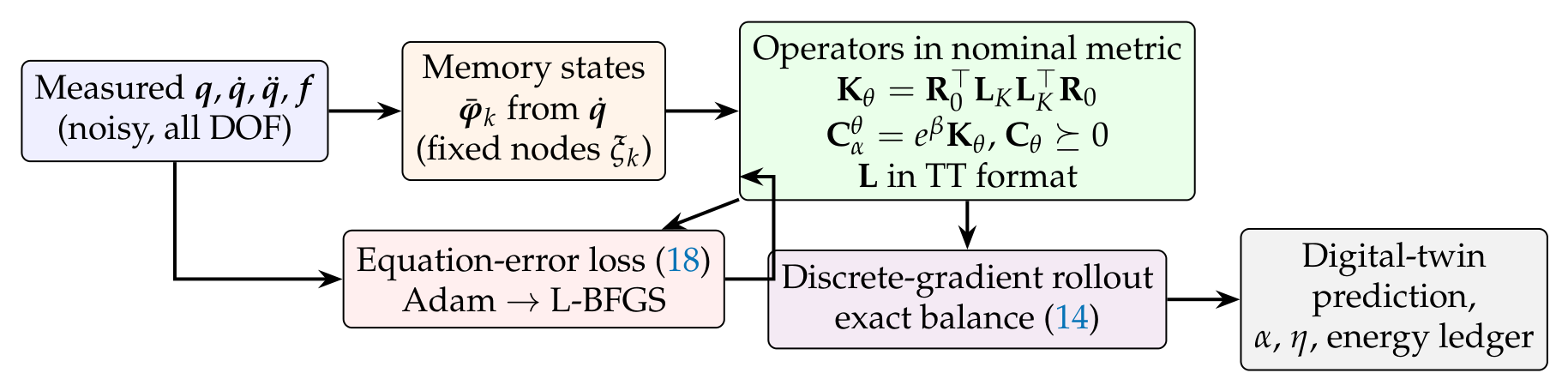
Figure 2.
E0, SDOF fractional oscillator. (a) Relative error of the diffusive pH solution () against the Newmark/L1 full-history reference () for three orders and three quadratures. (b) Maximum relative error of the quadrature transfer function with respect to ; the kernel errors for and agree to seven digits, so their curves overlap.
Figure 2.
E0, SDOF fractional oscillator. (a) Relative error of the diffusive pH solution () against the Newmark/L1 full-history reference () for three orders and three quadratures. (b) Maximum relative error of the quadrature transfer function with respect to ; the kernel errors for and agree to seven digits, so their curves overlap.
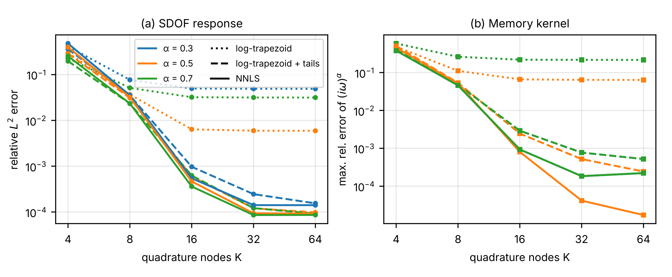
Figure 3.
E0, . (a) Displacement of the SDOF oscillator: Newmark/L1 reference and diffusive pH model with NNLS nodes (relative difference ). (b) Absolute residual of the discrete energy balance per step for the discrete-gradient integrator; RK4 overflows at the same step.
Figure 3.
E0, . (a) Displacement of the SDOF oscillator: Newmark/L1 reference and diffusive pH model with NNLS nodes (relative difference ). (b) Absolute residual of the discrete energy balance per step for the discrete-gradient integrator; RK4 overflows at the same step.
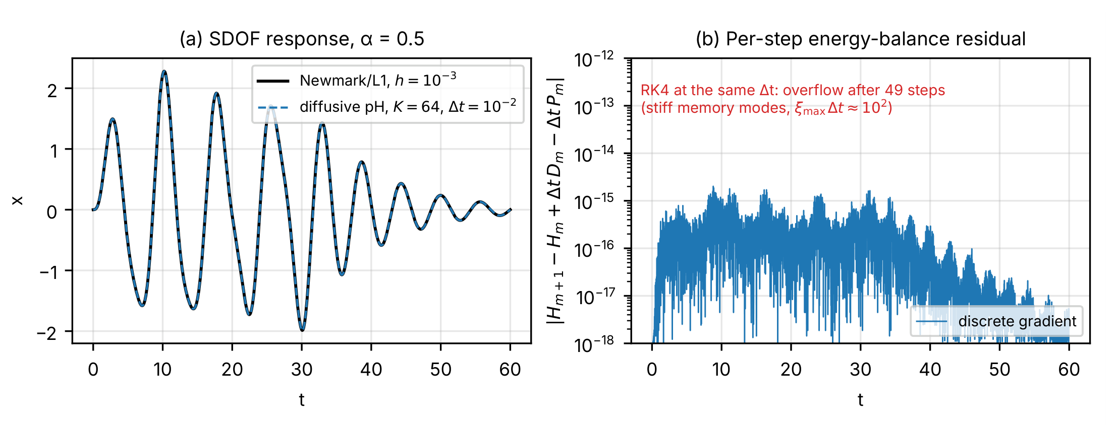
Figure 4.
E1: identified fractional order for the material-proportional (blue) and free (red) memory forms. Green boxes mark the acceptance band of H3; boxes are offset horizontally for readability.
Figure 4.
E1: identified fractional order for the material-proportional (blue) and free (red) memory forms. Green boxes mark the acceptance band of H3; boxes are offset horizontally for readability.
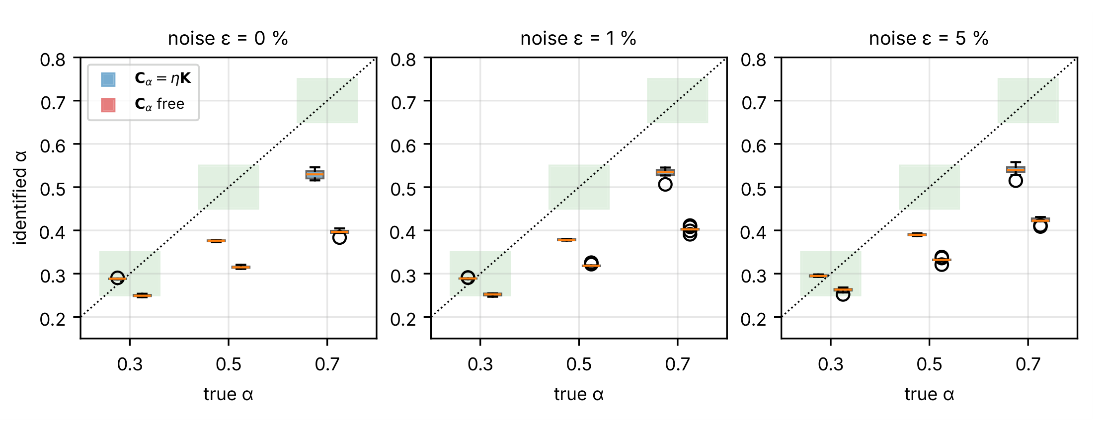
Figure 5.
E2 on the single-span truss (, , float32). (a) Smallest eigenvalue of the symmetric part of the learned stiffness after materialisation; the exact value of every structured model is non-negative, and the nondimensional spectrum of the true structure starts at one. (b) Trainable parameters. Rank 2 failed at the Cholesky factorisation and rank 32 exceeded the 90% memory cap of the GPU.
Figure 5.
E2 on the single-span truss (, , float32). (a) Smallest eigenvalue of the symmetric part of the learned stiffness after materialisation; the exact value of every structured model is non-negative, and the nondimensional spectrum of the true structure starts at one. (b) Trainable parameters. Rank 2 failed at the Cholesky factorisation and rank 32 exceeded the 90% memory cap of the GPU.
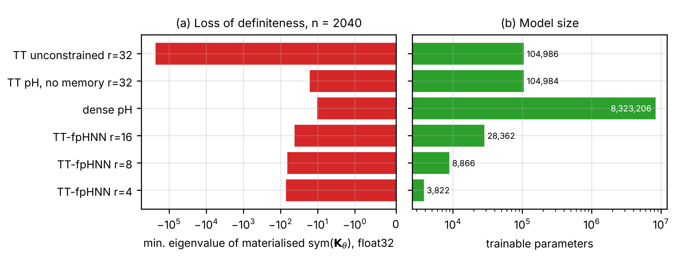
Figure 6.
E2 on the multi-span truss. (a) Midspan displacement of test trajectory T0 between periods 150 and 160, during the forced phase. (b) Relative error over 200 periods against the number of trainable parameters; small filled circles are individual training seeds, open circles their mean, and the square is the dense model with ridge. All structured models have .
Figure 6.
E2 on the multi-span truss. (a) Midspan displacement of test trajectory T0 between periods 150 and 160, during the forced phase. (b) Relative error over 200 periods against the number of trainable parameters; small filled circles are individual training seeds, open circles their mean, and the square is the dense model with ridge. All structured models have .
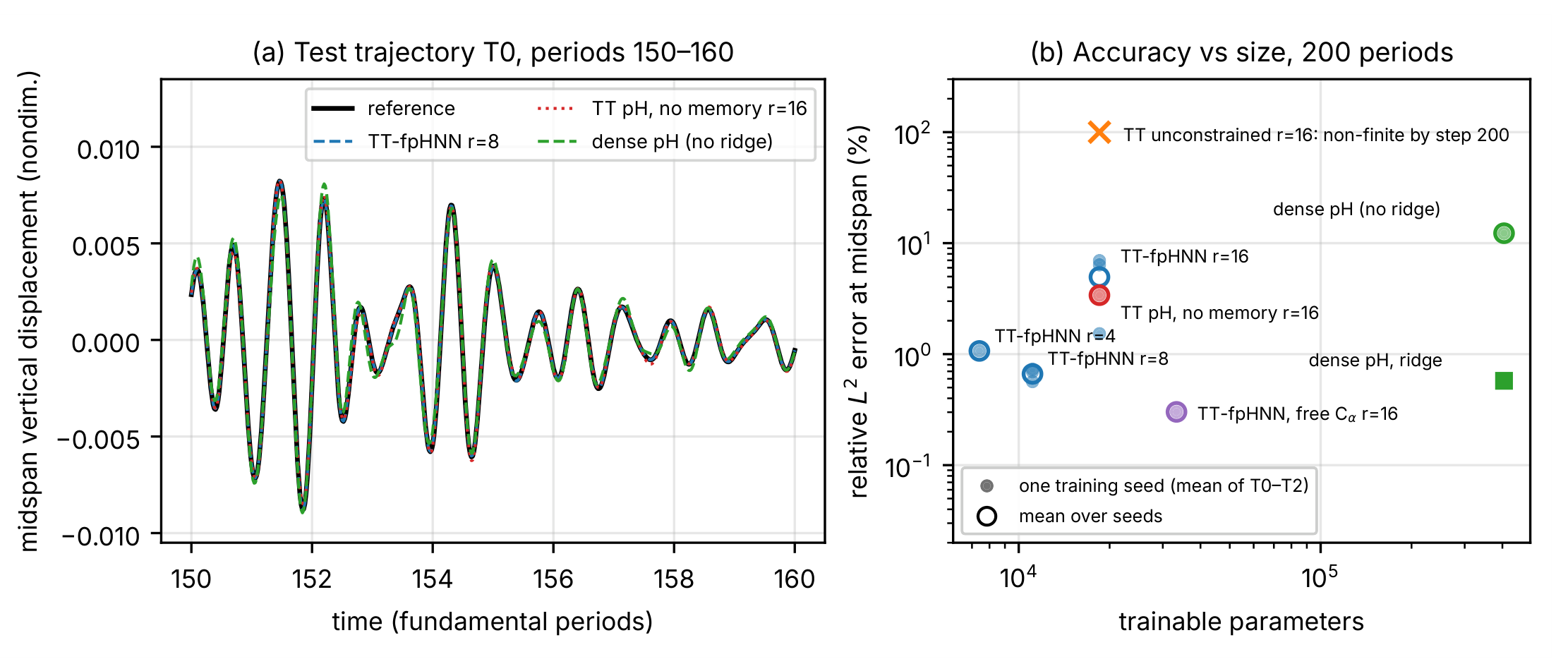
Figure 7.
E3, known 468-DOF system with . (a) Wall time per step for the diffusive pH scheme (, including the evaluation of energy and dissipation) and for Newmark/L1 with full and truncated history. (b) Relative error of the midspan displacement after 25 periods at , measured against two independent fine solutions computed with , which differ from each other by .
Figure 7.
E3, known 468-DOF system with . (a) Wall time per step for the diffusive pH scheme (, including the evaluation of energy and dissipation) and for Newmark/L1 with full and truncated history. (b) Relative error of the midspan displacement after 25 periods at , measured against two independent fine solutions computed with , which differ from each other by .
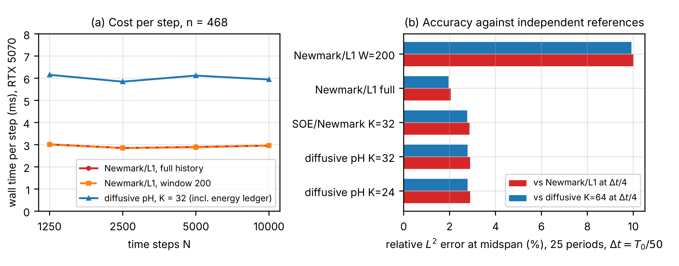
Table 1.
Structures used in the experiments. Frequencies are those of the physical model before nondimensionalisation; is the ratio of extreme eigenvalues of .
Table 1.
Structures used in the experiments. Frequencies are those of the physical model before nondimensionalisation; is the ratio of extreme eigenvalues of .
| Experiment | Bays | Supports | n | (Hz) | |
|---|---|---|---|---|---|
| E1 identifiability | 6 | ends | 60 | 15.24 | |
| E3 memory benchmark | 40 | ends | 468 | 0.55 | |
| E2 multi-span (float64) | 40 | ends + 3 piers | 450 | 5.16 | |
| E2 multi-span (float64) | 190 | ends + 18 piers | 2160 | 5.00 | |
| E2 single span (float32) | 171 | ends | 2040 | 0.031 |
Table 2.
E1: bias of the identified order (mean over 10 realisations) and fraction of realisations within (in parentheses). 60-DOF truss, 2500 Adam epochs and 40 L-BFGS steps.
Table 2.
E1: bias of the identified order (mean over 10 realisations) and fraction of realisations within (in parentheses). 60-DOF truss, 2500 Adam epochs and 40 L-BFGS steps.
| Memory form | ||||
|---|---|---|---|---|
| 0.3 | (1.0) | (1.0) | (1.0) | |
| 0.5 | (0.0) | (0.0) | (0.0) | |
| 0.7 | (0.0) | (0.0) | (0.0) | |
| free | 0.3 | (0.4) | (0.7) | (1.0) |
| 0.5 | (0.0) | (0.0) | (0.0) | |
| 0.7 | (0.0) | (0.0) | (0.0) |
Table 3.
E1 follow-up with excitation band , material-proportional memory, three realisations: bias of the identified order, fraction within (in parentheses), and relative error of the loss factor of Eq. (3).
Table 3.
E1 follow-up with excitation band , material-proportional memory, three realisations: bias of the identified order, fraction within (in parentheses), and relative error of the loss factor of Eq. (3).
| bias | error | bias | error | bias | error | |
| 0.3 | (1.0) | (1.0) | (0.0) | |||
| 0.5 | (1.0) | (1.0) | (0.0) | |||
| 0.7 | (1.0) | (1.0) | (1.0) | |||
Table 4.
E2 on the multi-span truss (, , , 1% noise, float64, rollouts of 10 000 steps, i.e. 200 fundamental periods). Error: relative error of the midspan displacement, mean over three test trajectories; for three seeds, mean over seeds with the range of the seed means in parentheses, otherwise the range over trajectories. : smallest eigenvalue of the learned stiffness (true value 1). The per-step balance residual of every structured rollout is below and its passivity violation is zero.
Table 4.
E2 on the multi-span truss (, , , 1% noise, float64, rollouts of 10 000 steps, i.e. 200 fundamental periods). Error: relative error of the midspan displacement, mean over three test trajectories; for three seeds, mean over seeds with the range of the seed means in parentheses, otherwise the range over trajectories. : smallest eigenvalue of the learned stiffness (true value 1). The per-step balance residual of every structured rollout is below and its passivity violation is zero.
| Model | Parameters | Seeds | Error (%) | OOD (%) | |||
|---|---|---|---|---|---|---|---|
| TT-fpHNN | 7406 | 1 | 1.07 (0.88–1.30) | 1.01 | 0.93 | 0.276 | 0.158 |
| TT-fpHNN | 11 106 | 3 | 0.66 (0.57–0.73) | 0.70 | 0.46–0.95 | 0.329–0.340 | 0.126–0.131 |
| TT-fpHNN | 18 506 | 3 | 4.95 (1.53–6.96) | 2.40 | 0.005–0.012 | 0.413–0.414 | 0.096–0.097 |
| TT-fpHNN, free , | 33 305 | 1 | 0.30 (0.25–0.39) | 0.16 | 0.99 | 0.397 | – |
| Dense pH, no ridge | 405 006 | 1 | 12.3 (8.4–15.7) | 14.9 | 0.021 | 0.619 | 0.056 |
| Dense pH, ridge | 405 006 | 1 | 0.58 (0.52–0.64) | 0.37 | 1.01 | 0.501 | 0.070 |
| TT pH without memory, | 18 504 | 1 | 3.40 (2.74–4.47) | 2.64 | 0.0015 | – | – |
| Unconstrained operators, | 18 506 | 1 | non-finite | non-finite | 0.377 | 0.111 |
Table 5.
Known 468-DOF system, , 25 periods at , 32 NNLS memory nodes in both schemes. Error: relative error at midspan against the fine L1 and fine diffusive references (). Ledger: residual of (14); cumulative value relative to .
Table 5.
Known 468-DOF system, , 25 periods at , 32 NNLS memory nodes in both schemes. Error: relative error at midspan against the fine L1 and fine diffusive references (). Ledger: residual of (14); cumulative value relative to .
| Scheme | Error vs L1 fine | Error vs diffusive fine | Max. ledger residual | Cumulative |
|---|---|---|---|---|
| Discrete-gradient pH (proposed) | 2.89% | 2.79% | ||
| SOE memory, exponential update, Newmark | 2.87% | 2.77% | ||
| Newmark/L1, full history | 2.05% | 1.96% | – | – |
Table 6.
Sensitivity to on the known 468-DOF system (tail-corrected log-trapezoidal rule, , ). Kernel error: maximum relative error of the transfer function on . Trajectory errors against the fine L1 reference.
Table 6.
Sensitivity to on the known 468-DOF system (tail-corrected log-trapezoidal rule, , ). Kernel error: maximum relative error of the transfer function on . Trajectory errors against the fine L1 reference.
| Amplification | Kernel error | Error, discrete gradient | Error, SOE/Newmark | |
|---|---|---|---|---|
| 1.26 | 1.41 | 3.51% | 3.47% | |
| 12.6 | 0.18 | 2.92% | 2.89% | |
| 126 | 2.90% | 2.87% | ||
| 1257 | 2.90% | 2.88% |
Table 7.
Measured comparison of TT-fpHNN with the baselines. Sources: E3 and its additional checks (, known operators), E2 on the multi-span truss (, 200 periods; TT-fpHNN with , mean of three seeds), E2 on the single span (, parameter counts only). “–” means the quantity does not exist for that baseline.
Table 7.
Measured comparison of TT-fpHNN with the baselines. Sources: E3 and its additional checks (, known operators), E2 on the multi-span truss (, 200 periods; TT-fpHNN with , mean of three seeds), E2 on the single span (, parameter counts only). “–” means the quantity does not exist for that baseline.
| Baseline (class) | Metric | Proposed | Baseline | Reading |
|---|---|---|---|---|
| SOE memory with Newmark (fast-convolution class [6,7]) | stored memory, | 120 kB | 120 kB | equal |
| error at 25 periods | 2.89% | 2.87% | equal | |
| energy-ledger residual per step | exact balance only for the proposed scheme | |||
| cumulative imbalance / injected energy | ||||
| History convolution, Newmark/L1 (discretisation used by fPINNs [4,15]) | stored memory after steps | 120 kB | 37 MB | baseline grows by bytes per step |
| error at 25 periods | 2.8–2.9% | 2.0–2.1% | proposed is less accurate at equal | |
| GPU time per step | 5.8–6.2 ms | 2.9–3.0 ms | proposed is slower at this size | |
| Short-memory L1, window of 200 steps | error at 25 periods | 2.8–2.9% | 9.9–10.0% | lower error at bounded cost |
| Unconstrained operator model (same loss, data and size) | error over 200 periods | 0.66% | non-finite | baseline diverges before step 200 |
| of learned stiffness | 0.46–0.95 | passivity by construction | ||
| pH network without memory (class of [24,27]) | error over 200 periods | 0.66% | 3.40% | lower error; ranks differ (8 and 16), see Section 5.4 |
| material loss factor at | to | – | baseline has no memory parameters | |
| Dense pH network with memory, ridge | trainable parameters, | 11 106 | 405 006 | fewer |
| trainable parameters, (–16) | 3822–28 362 | 8 323 206 | 293– fewer | |
| error over 200 periods | 0.66% | 0.58% | no accuracy gain | |
| identified order () | 0.33–0.34 | 0.501 | baseline identifies |
Disclaimer/Publisher’s Note: The statements, opinions and data contained in all publications are solely those of the individual author(s) and contributor(s) and not of MDPI and/or the editor(s). MDPI and/or the editor(s) disclaim responsibility for any injury to people or property resulting from any ideas, methods, instructions or products referred to in the content. |
© 2026 by the authors. Licensee MDPI, Basel, Switzerland. This article is an open access article distributed under the terms and conditions of the Creative Commons Attribution (CC BY) license (http://creativecommons.org/licenses/by/4.0/).
Copyright: This open access article is published under a Creative Commons CC BY 4.0 license, which permit the free download, distribution, and reuse, provided that the author and preprint are cited in any reuse.