
Submitted:
11 November 2026
Posted:
17 November 2026
You are already at the latest version
Abstract
Machine-learning optimisation of vertical Bridgman growth of CdTe is investigated using 2
an in-house axisymmetric conduction–thermoelastic solver. Six process and geometry 3
inputs were sampled with a 400-run Latin hypercube and an independent 60-run test set. 4
Gaussian process regression (GPR) and a multilayer perceptron outperformed random 5
forest and gradient boosting. In five-fold cross-validation, GPR gave coefficients of de- 6
termination of 0.995 for interface deflection (root-mean-square error 0.047 cm) and 0.975 7
for maximum von Mises stress (0.024 MPa). Sobol indices identified radius, cold-zone 8
undercooling and growth rate as dominant controls on deflection. Three-objective non- 9
dominated sorting genetic algorithm II optimisation, followed by two infill rounds and 10
solver verification, reduced mean absolute surrogate errors at Pareto points from 0.130 to 11
0.002 cm for deflection and from 0.036 to 0.011 MPa for stress. Direct Bayesian optimisation 12
found, within 40 runs, a design at 1 mm/h that reduced deflection magnitude from 1.335 to 13
0.554 cm and maximum stress from 0.339 to 0.243 MPa. Slightly convex fronts occurred only 14
below about 0.2 mm/h. The verified process windows are conditional on a conduction-only, 15
quasi-steady, isotropic model; absolute stresses retain mesh uncertainty of about 10%.
Keywords:
vertical Bridgman
; cadmium telluride
; machine learning
; Gaussian process regression
; Bayesian optimisation
; NSGA-II
; thermal stress
; interface shape
1. Introduction
Cadmium telluride (CdTe) and the related II–VI tellurides, in particular Cd1−xZnxTe (CZT), are key materials for thin-film photovoltaics [1] and for room-temperature X- and -ray detectors [2]. Bulk single crystals are mostly grown from the melt in sealed ampoules by the vertical Bridgman (VB) or vertical gradient freeze (VGF) methods [3,4]. The growth of large CdTe single crystals is notoriously difficult [3]: the thermal conductivity of CdTe is low (about 1.3–1.6 W/(m K) at the melting point [5]), and its resistance to plastic deformation at high temperature, measured for CdZnTe by Parfeniuk et al. [6], is limited. Two thermal quantities are therefore at the centre of process design: the shape of the crystal/melt interface, which should be flat or slightly convex toward the melt to avoid parasitic nucleation at the ampoule wall [7,8,9], and the thermoelastic stress in the growing crystal, which drives the multiplication of dislocations [6,10,11].
The usual route to process optimisation is a parametric study with a numerical model, one parameter at a time. For CZT and CdTe this has been done for the furnace temperature gradient [12], the interface shape [13], the thermal environment of the ampoule [8,14], the evolution of the interface during VGF growth [15], a thermal shielding ring [16], accelerated crucible rotation technique (ACRT) [17], melt vibrations [5] and double-diffusive convection [18]. Peterson and Derby proposed a criterion on the curvature of the axial temperature profile for the design of convex interfaces [9]. Such one-factor studies are informative but they do not explore the interactions between parameters, and the number of simulations needed to map a multi-dimensional process window grows quickly.
Machine learning (ML) offers data-efficient alternatives. Its applications to crystal growth have been reviewed by Dropka and Holena [19], Kutsukake [20] and Petkovic et al. [21]. For VGF growth of GaAs, neural networks have been used for real-time prediction of the growth dynamics [22] and for the inverse design of growth recipes [23], and model-based control has been developed [24]. In SiC solution growth, ML-accelerated predictions have been combined with adaptive process control [25] and with a genetic algorithm to optimise the flow distribution [26]. Physics-informed neural networks have been used to predict the melt flow and thermal fields in Czochralski growth of silicon [27,28], surrogate models combined with evolutionary or Shapley additive explanation (SHAP)-based analyses have been applied to Czochralski thermal fields [29,30], and Bayesian optimisation (BO) has been used to estimate a melt diffusion coefficient [31]. Closest to the present problem, Asakura et al. combined crystal growth simulation with feasibility-constrained BO to minimise the von Mises stress and maximise the interface convexity in Bridgman growth of Mg2Si [32]. For the tellurides, the only ML-driven optimisation we are aware of is that of Huang et al., who trained a Gaussian process regression model on about one hundred experimental travelling heater method (THM) runs of CZT to find optimal growth temperature, gradient and rate [33]; THM growth of CdTe is also the subject of recent global simulations [34]. The present work investigates ML-driven optimisation of VB growth of CdTe.
The present work addresses this gap for CdTe with a deliberately transparent, reproducible approach. An in-house axisymmetric conduction–thermoelastic solver is used as the physics model. A Latin-hypercube design over six process and geometry parameters provides the training data for four surrogate models (Gaussian process regression, random forest, gradient boosting and a multilayer perceptron). The best surrogate is used for a global sensitivity analysis and for multi-objective optimisation with the non-dominated sorting genetic algorithm II (NSGA-II), and a Bayesian optimisation is run directly on the solver. Every optimal point reported is re-computed with the solver, and the surrogate-versus-solver errors are given. The aim is to identify process windows that combine a flat interface, a low thermal stress and a high growth rate, and to state clearly what such a conduction-only model can and cannot predict.
2. Materials and Methods
2.1. Conduction–Thermoelastic Model
The charge is a cylinder of radius R and length L = 8 cm in a quasi-steady VB configuration (Figure 1). Heat is transferred by conduction in the crystal and melt, with conductivities and of CdTe at the melting point:
The interface is the isotherm T = , and the latent heat released at the translation rate v enters through the Stefan condition:
The furnace and ampoule are represented by a prescribed wall temperature: T = = − at the bottom, T = = + GL at the top, symmetry on the axis and
G is the nominal axial furnace gradient, the undercooling of the cold zone below , the position of the start of the gradient (adiabatic/booster) zone relative to the bottom of the ampoule, which plays the role of the growth stage, and the length of the gradient zone. The wall reaches at = + /(GL). The interface deflection is = (0) − (R); < 0 for a front concave toward the crystal and > 0 for a front convex toward the melt.
The crystal is linear-elastic, isotropic and stress-free at , with a traction-free surface. With the thermal strain (T−), the axisymmetric Navier equations
are solved with . The von Mises stress is . The CdTe properties are listed in Table 1.
2.2. Numerical Solver and Verification
The computations use an in-house axisymmetric conduction–thermoelastic solver, implemented by the authors and benchmarked against a reference Fortran implementation. Equation (1) is discretised by finite volumes on a uniform grid of step h with harmonic averaging of the thermal conductivity.
The phase is identified by a smoothed liquid fraction and the latent heat is released as the volumetric source v∂ /∂z. The non-linear problem is solved by Picard iterations with a direct sparse solver (under-relaxation 0.5, reduced to 0.2 and 0.1 if needed; tolerance ∘ C). The interface is located in each grid column by linear interpolation of the first upward crossing of , as in the reference implementation. Equation (4) is solved in weak form with four-node bilinear axisymmetric finite elements on the same grid, with a very soft, strain-free material in the melt. The solver reproduces the temperatures of the reference implementation to within 0.052 ∘ C and its interface position to within 0.004 cm, and an analytical thermoelastic solution for a long cylinder to within 1.90 % of the peak stress at h = 0.05 cm. A run takes 1–20 s on one CPU core.
2.3. Workflow, Design Variables and Data Generation
The workflow is summarised in Figure 2.
Six inputs are varied within the bounds of Table 2: the furnace gradient G, the translation (growth) rate v, the start and length of the gradient zone, the cold-zone undercooling and the charge radius R. The bounds keep the hot end above (GL > ). The upper rate, 2 mm/h, is the highest rate for which steady solutions were obtained without difficulty in the reference computations; at 5 and 10 mm/h the Picard iterations did not converge. For each run the solver returns the interface deflection , the maximum von Mises stress in the crystal max , the von Mises stress at the interface centre (one mesh step below (0)), the axial temperature gradient on the axis at the interface ∂T /∂z| (0), the crystal height on the axis (0), and the existence of a converged steady solution with a crystal on the axis.
A Latin-hypercube design [38] with 400 points, optimised for its centred discrepancy, provides the training set, and an independent Latin hypercube of 60 points the test set. The radius is rounded to the grid (h = 0.05 cm) before each run, and the rounded value is used as the input. The 460 runs took 15 CPU-minutes in total on 7 cores of a workstation. All runs converged and all had a crystal on the axis ( (0) ≥ 0.23 cm), so the existence of a steady solution is not a discriminating output in this design space and is not modelled further. A mesh check was made on 12 additional Latin-hypercube points with h = 0.1, 0.05 and 0.025 cm (radius on a 0.1 cm grid so that the three meshes have the same geometry).
2.4. Surrogate Models
Four regressors were trained separately for each output, with the inputs scaled to [0, 1] (scikit-learn implementation): (i) Gaussian process regression (GPR) with a Matérn-5/2 kernel with one length scale per input (automatic relevance determination) plus a white-noise term, hyperparameters by maximum marginal likelihood [39]; (ii) a random forest (RF) of 500 trees [40]; (iii) gradient boosting (GB) of 1000 trees of depth 4, learning rate 0.03, subsampling 0.8 [41]; (iv) a multilayer perceptron (MLP) with two hidden layers of 64 tanh neurons, L-BFGS training, penalty and standardised targets. The accuracy is measured by 5-fold cross-validation (CV) on the 400 training runs and on the independent test set, with the coefficient of determination , the root-mean-square error (RMSE) and the mean absolute error (MAE). Learning curves are obtained by training on random subsets of N = 25 to 400 runs (three repetitions) and testing on the 60 test runs.
2.5. Sensitivity Analysis
First-order () and total () Sobol indices are computed on the GPR surrogates with the Saltelli sampling scheme and the Jansen estimator [42] as implemented in SALib [43] (4096 × (6 + 2) surrogate evaluations, 95% bootstrap confidence intervals). As a model-independent check, permutation importances of a random forest are computed on the test set.
2.6. Optimisation and Verification
Multi-objective optimisation. At the reference radius R = 2 cm, three objectives are considered: minimise max , minimise |− | with the target = +0.05 cm (a slightly convex front, /R = 0.025), and maximise v. The constraint (0) ≥ 1.5 cm keeps the front away from the isothermal bottom of the charge, where an artificially flat front and a very short, nearly stress-free crystal would otherwise be obtained. The problem is solved with NSGA-II [44] (pymoo, population 200, 250 generations) on the GPR surrogates. All 200 points of the final population are re-computed with the solver. Because the optima lie on the boundaries of the design space, where the Latin hypercube is sparse, two infill rounds were made: the verified points were added to the training set, the GPR models were re-fitted and NSGA-II was run again. The front finally reported is the set of non-dominated points among the solver results. In addition, two-objective fronts (max , |− |) were computed at fixed v (0.25 to 2 mm/h) and R (1 to 2.5 cm), and 10 points of each were verified.
Bayesian optimisation. A scalar objective is defined with the reference design of Table 2 at v = 0 (uniform thermal conductivity, reference implementation, max = 0.1734 MPa, = −0.3183 cm) as normalisation:
J is minimised over (G, , , ) at v = 1 mm/h and R = 2 cm. BO with a GP prior (Matérn-5/2) and the expected-improvement acquisition [39] is run directly on the solver, starting from 8 Latin-hypercube runs and adding 32 sequential proposals. For comparison, J is also minimised on the final GPR surrogates by differential evolution, and the optimum is re-computed with the solver.
3. Results and Discussion
3.1. Dataset and Mesh Check
Figure 3 summarises the 400 training runs. The deflection ranges from −3.86 to +0.02 cm: in this conduction-only model the front is concave toward the crystal for all but one sampled design, and it becomes deeper with the growth rate and with the radius (Figure 3a), in agreement with the latent-heat effect found in the reference computations (from −0.420 cm at v = 0 to −2.368 cm at 2 mm/h for the reference design). The maximum von Mises stress ranges from 0.087 to 0.850 MPa and decreases markedly when the cold-zone undercooling is increased (Figure 3b).
The mesh check (Figure 4) shows that the interface quantities are mesh-converged at h = 0.05 cm: the mean difference with h = 0.025 cm is 0.0054 cm for (0.55 %) and the largest is 0.009 cm. The stresses converge more slowly: the mean relative difference of max is 7.4 % (largest 14.6 %) and that of , which is evaluated one mesh step below the front, 11.8 %. The maximum is located either just below the tip of the front on the axis or at the kink of the wall profile (R, ), where the stress has a weak singularity and grows slowly with refinement, as found for the reference design. The ranking of the designs is nevertheless preserved (Spearman rank correlation 0.986 for max and 0.993 for between h = 0.05 and 0.025 cm), so the optimisation is meaningful, but the absolute stresses given below carry an uncertainty of the order of 10 %.
3.2. Accuracy of the Surrogate Models
The CV and test metrics are given in Table 3. GPR and MLP are clearly better than the tree ensembles for all outputs: for the deflection, the CV RMSE is 0.026 cm (MLP) and 0.047 cm (GPR) against 0.169 cm (GB) and 0.236 cm (RF). The stresses are less smooth functions of the inputs, because the location of the maximum jumps between the axis and the wall kink, and GPR is the best model for both (CV coefficient of determination = 0.975 and RMSE 0.024 MPa for max ; CV coefficient of determination = 0.983 for the interface-centre stress). The metrics on the independent test set are equal to or slightly better than the CV values, which shows that the models are not over-fitted. The parity plots of the GPR models (Figure 5) show no systematic bias; the scatter of max above 0.5 MPa, i.e. at high rate and large radius, is the largest. GPR, which also provides a predictive variance, is used for the sensitivity analysis and the optimisation below.
The learning curves (Figure 6) show that the test RMSE of GPR and MLP decreases steadily with N, without a plateau at 400 runs for the deflection, while that of the stress decreases more slowly above 100 runs. With 100 runs, GPR already predicts max with an RMSE of about 0.028 MPa, better than RF and GB with 400 runs. For a data-poor situation, such as a surrogate trained on expensive global furnace simulations or on growth experiments [33], GPR is therefore the most efficient choice among the models tested.
3.3. Global Sensitivity
The Sobol indices (Figure 7) rank the inputs in the same order as the permutation importances. The radius dominates the deflection ( = 0.46), followed by (0.27) and v (0.26); G (0.06), (0.08) and (0.01) are secondary. For max the four inputs (0.33), R (0.31), G (0.23) and v (0.23) are all important, while the growth stage has negligible influence ( = 0.002), in agreement with the weak dependence found in the reference computations (max = 0.170–0.174 MPa for = 1.5–4.5 cm). The sum of the first-order indices (0.88 for , 0.83 for max ) shows that interactions account for 12–17 % of the variance. The importance of is a key result: the undercooling of the cold zone shifts the point where the wall reaches , = + /(GL), upward into the gradient zone, and the front is then located where the wall profile is closer to the linear profile that gives flat isotherms. In practice, and G are set by the temperatures of the cold and hot zones of the furnace.
The response surfaces of Figure 8 illustrate these trends around the reference design. In the (G, v) plane (Figure 8a,b), the front deepens with both G and v, and the stress increases with both; the flattest, least-stressed corner is that of low gradient and low rate. In the (, R) plane (Figure 8c, d), the deflection decreases strongly with the radius, approximately as , and is reduced by a large undercooling. At fixed radius, the stress passes through a maximum at ≈ 1.5–2.5 ∘ C and decreases at larger undercooling (from 0.348 to 0.302 MPa between 2 and 4 ∘ C at R = 2 cm); the low stresses at = 1 ∘ C are accompanied by the deepest fronts.
3.4. Bayesian Optimisation on the Solver
The BO history is shown in Figure 9. The best of the 8 initial runs has J = 6.62, close to the reference design (J = 6.30: = −1.335 cm, max = 0.339 MPa). The expected-improvement proposals reduce J to 4.41 at the first proposal and to 3.43 after 13 evaluations; the best value, J = 3.300, is reached at the 23rd evaluation and is not improved by the remaining 17 proposals, which explore other regions. The optimum (design D1 in Table 4) is G = 0.75 ∘ C/cm, = 1.50 cm, = 2.00 cm and = 4.0 ∘ C. Compared with the reference design at the same rate of 1 mm/h, the deflection is reduced from −1.335 to −0.554 cm (by 59 %) and the maximum stress from 0.339 to 0.243 MPa (by 28 %). Two of the four variables are at their bounds (minimum G, maximum ): the optimum is a boundary optimum, and lower gradients or larger undercoolings, which are outside the explored range, may give further improvement.
The surrogate route, i.e. the minimisation of J on the final GPR models (trained on 1000 runs) by differential evolution, gives G = 0.75 ∘ C/cm, = 1.50 cm, = 1.50 cm and = 4.0 ∘ C with a predicted J = 3.282. Re-computed with the solver, J = 3.336 (error 1.6 %; : −0.4598 predicted, −0.4601 cm computed; max : 0.291 predicted, 0.301 MPa computed). Both routes lead to the same corner of the design space; the direct BO needed 40 solver runs, the surrogate route 1000 runs, but the latter also provides the whole multi-objective picture below. Without infill, the surrogate trained on the 400 LHS runs gave a much poorer optimum (Jsolver = 4.23 against a predicted 3.67), because the boundary region is poorly sampled.
3.5. Multi-Objective Optimisation and Verification
Figure 10b shows the effect of the infill rounds on the agreement between GPR and solver at the Pareto points. In round 0 (GPR trained on the 400 LHS runs), the mean absolute error is 0.130 cm for (largest 0.405 cm), 0.036 MPa for max and 0.170 cm for (0), and 35 of the 200 points violate the constraint (0) ≥ 1.5 cm when re-computed. The surrogate is then extrapolating to the corners of the design space (G≈ 0.75 ∘ C/cm, ≈ 4 ∘ C) where the optimal designs lie. After one infill round (600 runs) the errors fall to 0.0066 cm, 0.014 MPa and 0.0054 cm, and after the second round (800 runs) to 0.0017 cm (largest 0.017 cm), 0.011 MPa (largest 0.090 MPa) and 0.0017 cm, with 2 constraint violations. The error on the stress remains about seven times larger, in relative terms, than that on the deflection, consistent with the CV results and the mesh check.
Among the 562 verified designs of the three rounds that satisfy the constraint, 352 are non-dominated with respect to the solver values (Figure 10a). The front shows the expected conflict between growth rate and interface/stress quality: the lowest stresses (0.10–0.26 MPa) and flattest fronts ( between −0.53 and +0.09 cm) are obtained at v≤ 0.5 mm/h, whereas at 1.5–2 mm/h the maximum stress is 0.33–0.65 MPa and ≤−0.83 cm. A slightly convex front ( > 0, up to +0.125 cm) is obtained only for v≲ 0.19 mm/h, with G≈ 0.75 ∘ C/cm and ≈ 3.9–4 ∘ C. The non-dominated designs are concentrated at the low-gradient bound: 98 % have G≤ 0.80 ∘ C/cm and 83 % have ≥ 3.5 ∘ C, while and take values over their whole ranges, which confirms that these two variables matter little.
The two-objective fronts at fixed rate and radius are shown in Figure 11 (solver values of the 10 verified points per front). At R = 2 cm (Figure 11a), each 0.5 mm/h increase in rate shifts the front toward deeper interfaces and higher stresses. At v = 1 mm/h (Figure 11b), the attainable deflection and stress increase strongly with the radius: the best compromise moves from about (|− |, max ) = (0.33, 0.09) at R = 1 cm to (0.80, 0.19) at 2 cm and (1.15, 0.27) at 2.5 cm. For R≠ 2 cm, where no infill was made, the surrogate errors at these fronts are larger (MAE of 0.061 cm at R = 1 cm and 0.056 cm at R = 2.5 cm, against 0.0013 cm at R = 2 cm), which is why only solver values are plotted.
3.6. Optimal Designs and Process Windows
Three designs are compared with the reference design in Table 4 and Figure 12 and Figure 13: the BO optimum D1 (1 mm/h), the best verified Pareto design in terms of J at about 0.4 mm/h (D2) and that at v≥ 1.5 mm/h (D3). All values in the table were re-computed with the solver. Compared with the reference, the low-gradient, large-undercooling designs raise the interface on the axis relative to the wall and reduce its curvature (Figure 13a). The isotherm maps (Figure 12) show why: with = 4 ∘ C and G = 0.75 ∘ C/cm, the wall reaches well inside the gradient zone, where the isotherms are less curved. In D1 and D2 the maximum stress moves from the axis below the tip of the front (reference) to the wall kink at (R, ), where it is mesh-sensitive, and the stress along the axis is much lower (Figure 13b). Design D3 shows the price of a 50 % higher rate: the front is 0.28 cm deeper and the maximum stress 60 % higher than in D1.
From the verified Pareto set, the following process windows are recommended for a 4 cm diameter CdTe charge in the present model: (i) for a nearly flat front, |− | ≤ 0.5 cm, with max ≤ 0.25 MPa, the rate must not exceed about 0.83 mm/h, with G≈ 0.75 ∘ C/cm and ≈ 4 ∘ C; (ii) relaxing the limits to |− | ≤ 0.8 cm and max ≤ 0.35 MPa allows up to about 1.35 mm/h with the same furnace settings and a short gradient zone (≈ 1.6–2 cm); (iii) a slightly convex front requires v≲ 0.2 mm/h. In all cases, the lowest gradient and the largest cold-zone undercooling of the explored range are preferred, and the gradient-zone position and length can be chosen for other reasons. These windows agree qualitatively with the classical guidelines that the front shape is controlled by the thermal environment near the interface [7,8,9]; the new elements are the quantified trade-off with the growth rate and the dominant role of the cold-zone undercooling.
3.7. Limitations
The conclusions are bounded by the physics model. (i) Heat transfer is conduction only: melt convection, which modifies the heat flux at the front and its shape [14,18], and forced flows such as ACRT [17] or melt vibrations [5] are not represented. (ii) The furnace and ampoule are replaced by a prescribed wall temperature; a global model including the ampoule, its support and radiation [14,15,16] would change the effective boundary condition, and the design variables G, , and should be read as parameters of the wall profile rather than as furnace set-points. (iii) The problem is quasi-steady, and the growth stage is represented only through . (iv) The crystal is elastically isotropic; the Young’s modulus of CdTe varies from 23.5 GPa along to 51.7 GPa along , and the stresses are not converted to resolved shear stresses or dislocation densities [10,11]. (v) The thermal expansion coefficient is the value measured at 420 ∘ C [37], and the stresses carry a mesh uncertainty of about 10 %. (vi) The optima are at the bounds of the design space and the surrogate errors are largest there and for radii without infill. The method itself, LHS + GPR with infill + NSGA-II, BO and systematic solver verification, is independent of these limitations and can be applied unchanged to a higher-fidelity model.
4. Conclusions
Machine-learning optimisation of the vertical Bridgman growth of CdTe has been carried out with an in-house conduction–thermoelastic solver as the physics model. The main conclusions are:
- With 400 Latin-hypercube runs, GPR and MLP predict the interface deflection with CV coefficients of determination of at least 0.995; GPR predicts stresses with CV coefficients of determination of 0.975–0.983. These models outperform random forest and gradient boosting, and GPR is the most data-efficient model among those tested.
- The radius, the cold-zone undercooling and the growth rate dominate the deflection; the undercooling, radius, gradient and rate share the influence on the maximum stress, and the growth stage (position of the gradient zone) has none.
- The optima lie on the boundaries of the design space, where a surrogate trained on space-filling data alone is unreliable. Two infill rounds with solver verification reduced the error at the Pareto points from 0.130 to 0.002 cm (deflection) and from 0.036 to 0.011 MPa (stress).
- Bayesian optimisation directly on the solver found the optimum of a combined stress/deflection objective in 23 of 40 runs. At 1 mm/h, a low gradient (0.75 ∘ C/cm) and a large cold-zone undercooling (4 ∘ C) reduce the deflection by 59 % and the maximum stress by 28 % compared with the reference design.
- The verified Pareto front quantifies the trade-off with the growth rate: a nearly flat front (|− | ≤ 0.5 cm) with max ≤ 0.25 MPa is possible up to about 0.8 mm/h for a 4 cm charge, and a slightly convex front only below about 0.2 mm/h.
These results are valid within a conduction-only, quasi-steady, isotropic model with a prescribed wall temperature. The next steps are to use the same workflow with a global furnace model including melt convection and ACRT, anisotropic elasticity and a dislocation criterion, and to test the recommended windows experimentally.
Author Contributions
Azzeddine Bouroucha: Conceptualization, Methodology, Software, Formal analysis, Investigation, Visualization, Writing—original draft. Kamel Guergouri: Supervision, Validation, Writing—review & editing.
Funding
This research received no specific grant from any funding agency in the public, commercial, or not-for-profit sectors.
Institutional Review Board Statement
Not applicable.
Informed Consent Statement
Not applicable.
Data Availability Statement
The data supporting the reported results will be made available by the corresponding author on request.
Acknowledgments
The authors express their gratitude to the Department of Physics, Faculty of Exact Sciences at the University of Mentouri Brothers Constantine 1 (Constantine, Algeria) for providing a supportive research environment and continuous encouragement throughout this work.
Conflicts of Interest
The authors declare no conflict of interest.
Nomenclature and Abbreviations
| Cylindrical coordinates | |
| Charge radius and length | |
| Temperature and melting temperature | |
| Cold-end, hot-end and wall temperatures | |
| Cold-zone undercooling, | |
| G | Nominal axial furnace gradient |
| Start and length of the gradient zone | |
| Wall melting-isotherm position and interface position | |
| Interface deflection and its target | |
| Translation rate and mesh step | |
| Solid and melt thermal conductivities | |
| Solid density and latent heat of fusion | |
| Young’s modulus, Poisson’s ratio, thermal expansion coefficient | |
| Lamé constants | |
| Stress components, von Mises stress and interface-centre value | |
| Scalar objective, training-set size and determination coefficient | |
| First-order and total Sobol sensitivity indices | |
| BO, CV, DE | Bayesian optimisation; cross-validation; differential evolution |
| EI, GB, GPR | Expected improvement; gradient boosting; Gaussian process regression |
| LHS, MLP, RF | Latin hypercube sampling; multilayer perceptron; random forest |
| RMSE, MAE | Root-mean-square error; mean absolute error |
References
- Romeo, A.; Artegiani, E. CdTe-Based Thin Film Solar Cells: Past, Present and Future. Energies 2021, 14, 1684. [Google Scholar] [CrossRef]
- Alam, M.D.; Nasim, S.S.; Hasan, S. Recent progress in CdZnTe based room temperature detectors for nuclear radiation monitoring. Prog. Nucl. Energy 2021, 140, 103918. [Google Scholar] [CrossRef]
- Rudolph, P. Fundamental studies on Bridgman growth of CdTe. Prog. Cryst. Growth Charact. Mater. 1994, 29, 275–381. [Google Scholar] [CrossRef]
- Shi, Y.; Wang, P.; Mu, H.; Kou, H.; Wu, A.; Su, L. Advances of interface, flow, and stress control for VB crystal growth: An overview. Prog. Cryst. Growth Charact. Mater. 2023, 69, 100605. [Google Scholar] [CrossRef]
- Nefedov, O.; Dovnarovich, A.; Kostikov, V.; Mozhevitina, E.; Bocharnikov, D.; Avetissov, I. Numerical Simulation of CdTe Crystal Growth Using the Vertical Gradient Freeze Technique Assisted by Axial Low-Frequency Oscillations of the Melt. Crystals 2024, 14, 72. [Google Scholar] [CrossRef]
- Parfeniuk, C.; Weinberg, F.; Samarasekera, I.; Schvezov, C.; Li, L. Measured critical resolved shear stress and calculated temperature and stress fields during growth of CdZnTe. J. Cryst. Growth 1992, 119, 261–270. [Google Scholar] [CrossRef]
- Chang, C.E.; Wilcox, W.R. Control of interface shape in the vertical bridgman-stockbarger technique. J. Cryst. Growth 1974, 21, 135–140. [Google Scholar] [CrossRef]
- Kuppurao, S.; Derby, J.J. Designing thermal environments to promote convex interface shapes during the vertical Bridgman growth of cadmium zinc telluride. J. Cryst. Growth 1997, 172, 350–360. [Google Scholar] [CrossRef]
- Peterson, J.H.; Derby, J.J. An axial temperature profile curvature criterion for the engineering of convex crystal growth interfaces in Bridgman systems. J. Cryst. Growth 2017, 468, 899–904. [Google Scholar] [CrossRef]
- Jordan, A.S.; Caruso, R.; Von Neida, A.R. A Thermoelastic Analysis of Dislocation Generation in Pulled GaAs Crystals. Bell Syst. Tech. J. 1980, 59, 593–637. [Google Scholar] [CrossRef]
- Kakimoto, K.; Takahashi, I.; Tomida, T.; Kamada, K.; Yao, Y.; Nakano, S.; Yoshikawa, A. 3D calculation studies of dislocation density in a β-Ga2O3 crystal grown by vertical Bridgman method. J. Cryst. Growth 2023, 609, 127126. [Google Scholar] [CrossRef]
- Yan, B.; Liu, W.; Yu, C.; Yu, Z.; Shangguan, M.; Yan, J.; Huang, L. Optimizing the temperature gradient for CdZnTe crystal growth using the vertical Bridgman–Stockbarger method. J. Cryst. Growth 2023, 621, 127378. [Google Scholar] [CrossRef]
- Yan, B.; Liu, W.; Yu, C.; Gao, P.; Liang, T.; Liao, K.; Jiang, B.; Wang, T.; Liu, F.; Liang, H.; Feng, K.; Huang, L. Optimizing growth interface shape in CdZnTe single crystal growth using vertical Bridgman method. J. Cryst. Growth 2026, 676, 128456. [Google Scholar] [CrossRef]
- Stelian, C.; Calestani, D.; Velázquez, M.; Zappettini, A. Numerical and experimental investigation of CdZnTe growth by the boron oxide encapsulated vertical Bridgman method. Int. J. Heat Mass Transf. 2021, 176, 121490. [Google Scholar] [CrossRef]
- Li, S.; Zhou, C.; Xu, C. Evolution features and optimization of interface shape during CdZnTe crystal growth using Vertical Gradient Freeze (VGF) technique. J. Cryst. Growth 2024, 627, 127536. [Google Scholar] [CrossRef]
- Zhu, Z.; Ni, Y.; Yu, X.; Huang, C.; Wu, H.; Hu, Q.; Qi, H.; Li, Y.; Liu, G.; Yu, P.; Chen, W.; Zhang, Q. Numerical and experimental investigation of CdTe crystal growth assisted by a thermal–shielding ring for stable interface control. Mater. Sci. Semicond. Process. 2026, 201, 110059. [Google Scholar] [CrossRef]
- Divecha, M.S.; Derby, J.J. Optimizing ACRT to reduce inclusion formation during the VGF growth of cadmium zinc telluride: I. Computational approach. J. Cryst. Growth 2021, 576, 126386. [Google Scholar] [CrossRef]
- Gusev, A.O.; Denisov, I.A.; Mazhorova, O.S. Numerical Study of Interplay between Double-diffusive Convection and Interfacial Phenomena in Vertical Bridgman Crystal Growth of CdZnTe. Fluid Dyn. 2024, 59, 1888–1904. [Google Scholar] [CrossRef]
- Dropka, N.; Holena, M. Application of Artificial Neural Networks in Crystal Growth of Electronic and Opto-Electronic Materials. Crystals 2020, 10, 663. [Google Scholar] [CrossRef]
- Kutsukake, K. Review of machine learning applications for crystal growth research. J. Cryst. Growth 2024, 630, 127598. [Google Scholar] [CrossRef]
- Petkovic, M.; Vieira, L.; Dropka, N. Machine learning in crystal growth: A review of methods, data, and applications. Prog. Cryst. Growth Charact. Mater. 2025, 71, 100689. [Google Scholar] [CrossRef]
- Dropka, N.; Ecklebe, S.; Holena, M. Real Time Predictions of VGF-GaAs Growth Dynamics by LSTM Neural Networks. Crystals 2021, 11, 138. [Google Scholar] [CrossRef]
- Dropka, N.; Holena, M.; Thieme, C.; Chou, T. Development of the VGF Crystal Growth Recipe: Intelligent Solutions of Ill-Posed Inverse Problems using Images and Numerical Data. Cryst. Res. Technol. 2023, 58, 2300125. [Google Scholar] [CrossRef]
- Ecklebe, S.; Woittennek, F.; Frank-Rotsch, C.; Dropka, N.; Winkler, J. Toward Model-Based Control of the Vertical Gradient Freeze Crystal Growth Process. IEEE Trans. Control Syst. Technol. 2022, 30, 384–391. [Google Scholar] [CrossRef]
- Dang, Y.; Zhu, C.; Ikumi, M.; Takaishi, M.; Yu, W.; Huang, W.; Liu, X.; Kutsukake, K.; Harada, S.; Tagawa, M.; Ujihara, T. Adaptive process control for crystal growth using machine learning for high-speed prediction: application to SiC solution growth. CrystEngComm 2021, 23, 1982–1990. [Google Scholar] [CrossRef]
- Isono, M.; Harada, S.; Kutsukake, K.; Yokoyama, T.; Tagawa, M.; Ujihara, T. Optimization of Flow Distribution by Topological Description and Machine Learning in Solution Growth of SiC. Adv. Theory Simul. 2022, 5, 2200302. [Google Scholar] [CrossRef]
- Shi, S.; Liu, D.; Huo, Z. Simulation of flow field in silicon single-crystal growth using physics-informed neural network with spatial information. Phys. Fluids 2022, 34, 113610. [Google Scholar] [CrossRef]
- Takehara, Y.; Okano, Y.; Dost, S. Fast Prediction of Transport Structures in the Melt by Physics Informed Neural Networks during `VMCz’ Crystal Growth of Silicon. J. Chem. Eng. Jpn. 2023, 56, 2236656. [Google Scholar] [CrossRef]
- Peng, R.; Tang, H.; Wu, J. Multi-objective optimization of Magnetic Czochralski crystal growth process using surrogate modeling and evolutionary algorithm. Appl. Therm. Eng. 2026, 290, 130075. [Google Scholar] [CrossRef]
- Huang, Y.; Ansari Dezfoli, A.R.; Khaleghi, M.; Chaji, M.; Hadidchi, S. Integrated COMSOL–machine-learning–SHAP Framework for thermal-field optimization and interface stability analysis in Czochralski silicon growth. Int. J. Adv. Manuf. Technol. 2026. [Google Scholar] [CrossRef]
- Ghritli, R.; Okano, Y.; Inatomi, Y.; Sekimoto, A.; Dost, S. Estimation of the diffusion coefficient of GaSb in InSb melt using Bayesian optimization and the ISS experimental results. J. Cryst. Growth 2021, 573, 126280. [Google Scholar] [CrossRef]
- Asakura, K.; Kutsukake, K.; Kudo, H.; Katsube, R.; Udono, H.; Usami, N. Process optimization for Mg2Si single crystal growth using crystal growth simulation and Bayesian optimization with feasibility constraints. J. Cryst. Growth 2026, 694, 128788. [Google Scholar] [CrossRef]
- Huang, Y.; Tang, Z.; Zhang, K.; Zhang, B.; Gu, C.; Liu, K.; Liang, X.; Cao, M.; Wei, J.; Liu, W.; Zhang, J.; Wang, L. Machine learning optimization of CdZnTe crystal growth by the travelling heater method. J. Appl. Crystallogr. 2025, 58, 1899–1907. [Google Scholar] [CrossRef]
- Lan, C. Global dynamic simulation of the traveling heater method for CdTe crystal growth. J. Cryst. Growth 2026, 696, 128847. [Google Scholar] [CrossRef]
- McSkimin, H.J.; Thomas, D.G. Elastic Moduli of Cadmium Telluride. J. Appl. Phys. 1962, 33, 56–59. [Google Scholar] [CrossRef]
- Hill, R. The Elastic Behaviour of a Crystalline Aggregate. Proc. Phys. Soc. Sect. A 1952, 65, 349–354. [Google Scholar] [CrossRef]
- Williams, M.; Tomlinson, R.; Hampshire, M. X-ray determination of the lattice parameters and thermal expansion of cadmium telluride in the temperature range 20–420∘C. Solid State Commun. 1969, 7, 1831–1832. [Google Scholar] [CrossRef]
- McKay, M.D.; Beckman, R.J.; Conover, W.J. Comparison of Three Methods for Selecting Values of Input Variables in the Analysis of Output from a Computer Code. Technometrics 1979, 21, 239–245. [Google Scholar] [CrossRef]
- Garnett, R. Bayesian Optimization; Cambridge University Press: Cambridge, UK, 2023. [Google Scholar] [CrossRef]
- Breiman, L. Random Forests. Mach. Learn. 2001, 45, 5–32. [Google Scholar] [CrossRef]
- Friedman, J.H. Greedy function approximation: A gradient boosting machine. Ann. Stat. 2001, 29, 1189–1232. [Google Scholar] [CrossRef]
- Saltelli, A.; Annoni, P.; Azzini, I.; Campolongo, F.; Ratto, M.; Tarantola, S. Variance based sensitivity analysis of model output. Design and estimator for the total sensitivity index. Comput. Phys. Commun. 2010, 181, 259–270. [Google Scholar] [CrossRef]
- Iwanaga, T.; Usher, W.; Herman, J. Toward SALib 2.0: Advancing the accessibility and interpretability of global sensitivity analyses. Socio-Environ. Syst. Model. 2022, 4, 18155. [Google Scholar] [CrossRef]
- Deb, K.; Pratap, A.; Agarwal, S.; Meyarivan, T. A fast and elitist multiobjective genetic algorithm: NSGA-II. IEEE Trans. Evol. Comput. 2002, 6, 182–197. [Google Scholar] [CrossRef]
Figure 1.
(a) Schematic of vertical Bridgman growth and of the design variables, (b) computational domain and boundary conditions, (c) wall temperature profile (z) (not to scale)
Figure 1.
(a) Schematic of vertical Bridgman growth and of the design variables, (b) computational domain and boundary conditions, (c) wall temperature profile (z) (not to scale)
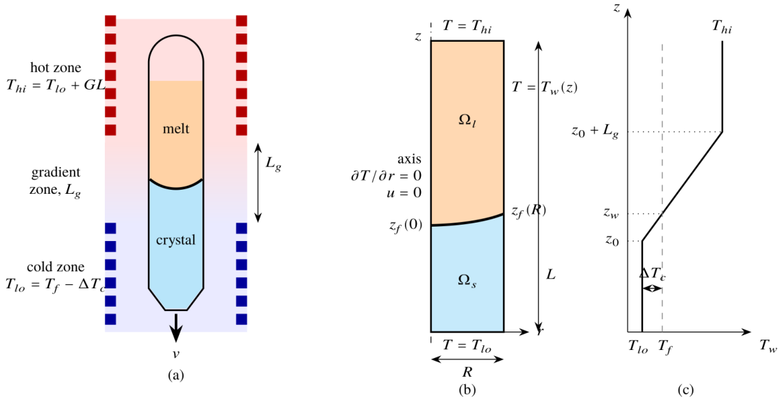
Figure 2.
Workflow of data generation, surrogate modelling, sensitivity analysis, optimisation and verification. FV: finite volume; FE: finite element; GPR: Gaussian process regression; RF: random forest; GB: gradient boosting; MLP: multilayer perceptron; CV: cross-validation; GP-EI: Gaussian process with expected improvement; NSGA-II: non-dominated sorting genetic algorithm II.
Figure 2.
Workflow of data generation, surrogate modelling, sensitivity analysis, optimisation and verification. FV: finite volume; FE: finite element; GPR: Gaussian process regression; RF: random forest; GB: gradient boosting; MLP: multilayer perceptron; CV: cross-validation; GP-EI: Gaussian process with expected improvement; NSGA-II: non-dominated sorting genetic algorithm II.
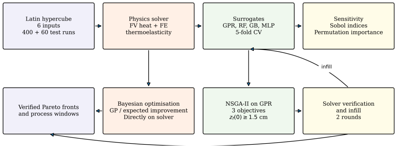
Figure 3.
Latin-hypercube training set (400 solver runs): (a) interface deflection versus growth rate (colour: radius), (b) maximum von Mises stress versus cold-zone undercooling (colour: furnace gradient)
Figure 3.
Latin-hypercube training set (400 solver runs): (a) interface deflection versus growth rate (colour: radius), (b) maximum von Mises stress versus cold-zone undercooling (colour: furnace gradient)
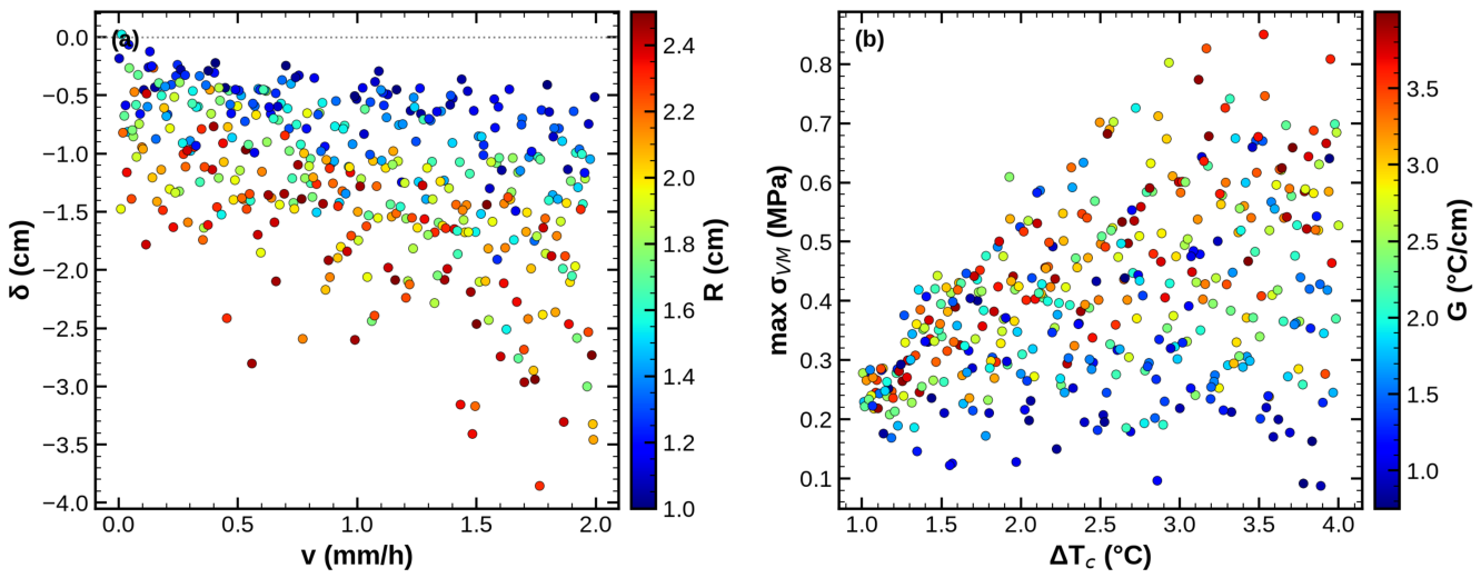
Figure 4.
Mesh check on 12 random designs: (a) deflection, (b) maximum von Mises stress computed with h = 0.1 and 0.05 cm versus h = 0.025 cm
Figure 4.
Mesh check on 12 random designs: (a) deflection, (b) maximum von Mises stress computed with h = 0.1 and 0.05 cm versus h = 0.025 cm
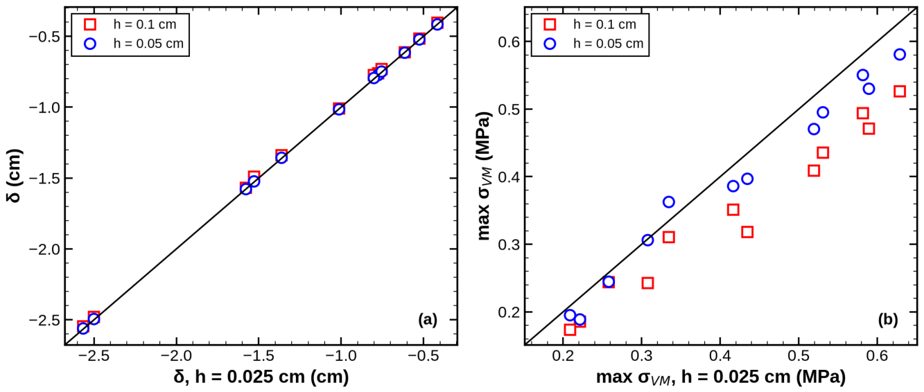
Figure 5.
Parity plots of the GPR surrogates (open circles: 5-fold CV predictions; squares: independent test set): (a) deflection, (b) maximum von Mises stress, (c) von Mises stress at the interface centre, (d) axial gradient on the axis at the interface
Figure 5.
Parity plots of the GPR surrogates (open circles: 5-fold CV predictions; squares: independent test set): (a) deflection, (b) maximum von Mises stress, (c) von Mises stress at the interface centre, (d) axial gradient on the axis at the interface
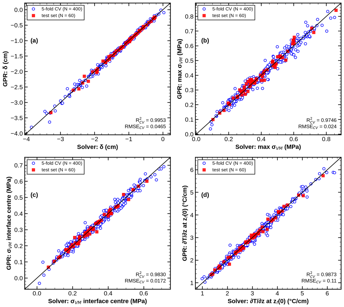
Figure 6.
Learning curves: test-set RMSE versus number of training runs (mean and standard deviation of three random subsets): (a) deflection, (b) maximum von Mises stress
Figure 6.
Learning curves: test-set RMSE versus number of training runs (mean and standard deviation of three random subsets): (a) deflection, (b) maximum von Mises stress
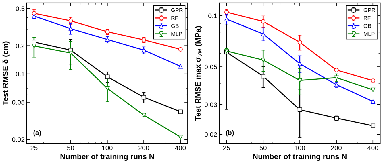
Figure 7.
Global sensitivity indices (Sobol first-order and total on the GPR surrogates, with 95% confidence intervals, and normalised random-forest permutation importance): (a) deflection, (b) maximum von Mises stress, (c) von Mises stress at the interface centre
Figure 7.
Global sensitivity indices (Sobol first-order and total on the GPR surrogates, with 95% confidence intervals, and normalised random-forest permutation importance): (a) deflection, (b) maximum von Mises stress, (c) von Mises stress at the interface centre
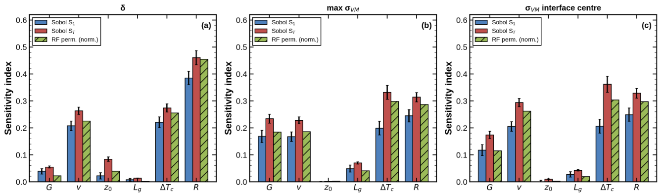
Figure 8.
GPR response surfaces around the reference design ( = 2.5 cm, = 3 cm; other variables as in Table 2): (a) deflection and (b) maximum von Mises stress versus G and v ( = 2 ∘ C, R = 2 cm); (c) deflection and (d) maximum von Mises stress versus and R (G = 1 ∘ C/cm, v = 1 mm/h)
Figure 8.
GPR response surfaces around the reference design ( = 2.5 cm, = 3 cm; other variables as in Table 2): (a) deflection and (b) maximum von Mises stress versus G and v ( = 2 ∘ C, R = 2 cm); (c) deflection and (d) maximum von Mises stress versus and R (G = 1 ∘ C/cm, v = 1 mm/h)
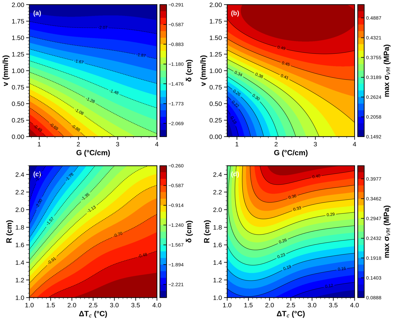
Figure 9.
Bayesian optimisation of the objective J (Equation 5) directly on the solver (v = 1 mm/h, R = 2 cm): objective of each evaluation and best value so far, compared with the solver-verified optimum of the GPR surrogate and with the reference design
Figure 9.
Bayesian optimisation of the objective J (Equation 5) directly on the solver (v = 1 mm/h, R = 2 cm): objective of each evaluation and best value so far, compared with the solver-verified optimum of the GPR surrogate and with the reference design
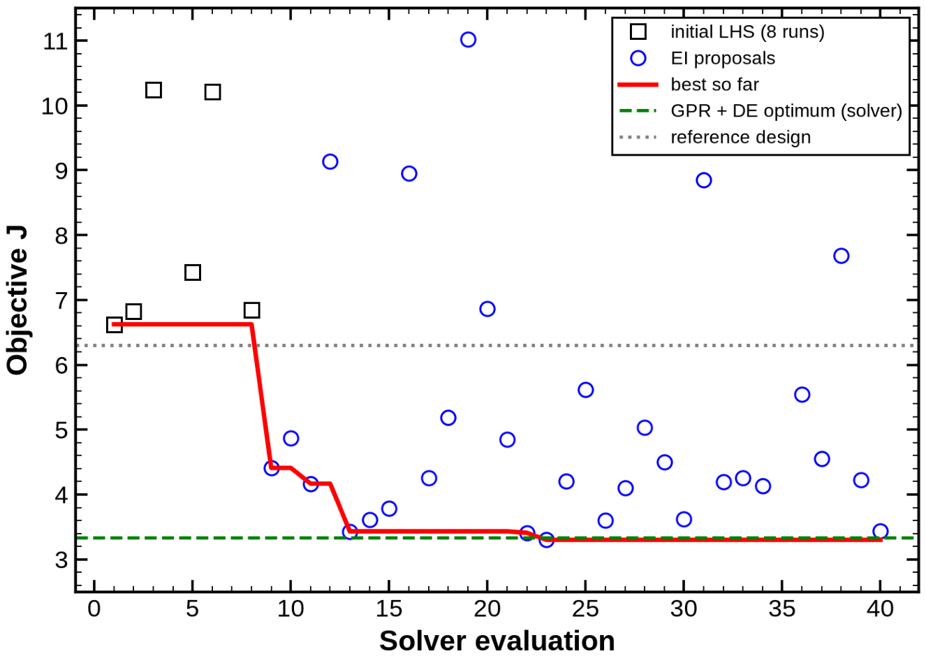
Figure 10.
Three-objective optimisation at R = 2 cm: (a) solver-verified non-dominated designs (352 points; colour: growth rate) in the plane (|− |, max ), (b) GPR versus solver deflection at the 200 Pareto points of infill rounds 0 and 2
Figure 10.
Three-objective optimisation at R = 2 cm: (a) solver-verified non-dominated designs (352 points; colour: growth rate) in the plane (|− |, max ), (b) GPR versus solver deflection at the 200 Pareto points of infill rounds 0 and 2
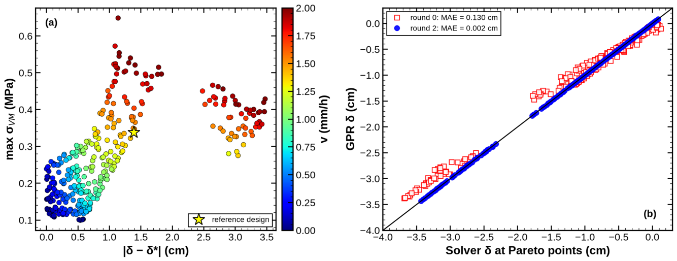
Figure 11.
Two-objective fronts (solver-verified): (a) for different growth rates at R = 2 cm, (b) for different radii at v = 1 mm/h. Lines: non-dominated verified points; small symbols: dominated verified points
Figure 11.
Two-objective fronts (solver-verified): (a) for different growth rates at R = 2 cm, (b) for different radii at v = 1 mm/h. Lines: non-dominated verified points; small symbols: dominated verified points
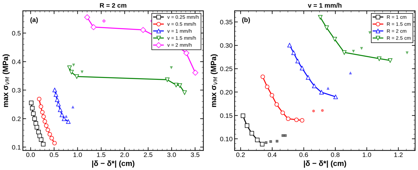
Figure 12.
Temperature (left half of each panel, 24 levels per panel; white line: T = ) and von Mises stress in the crystal (right half, common scale) for the reference design and the optimal designs D1–D3 of Table 4.
Figure 12.
Temperature (left half of each panel, 24 levels per panel; white line: T = ) and von Mises stress in the crystal (right half, common scale) for the reference design and the optimal designs D1–D3 of Table 4.
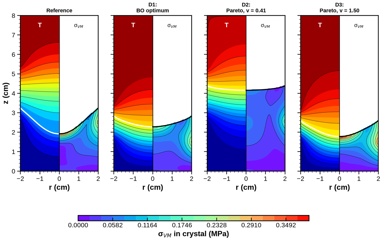
Figure 13.
Reference and optimal designs: (a) interface shape relative to the wall position, (b) von Mises stress along the axis (solid) and along the wall (dashed) in the crystal
Figure 13.
Reference and optimal designs: (a) interface shape relative to the wall position, (b) von Mises stress along the axis (solid) and along the wall (dashed) in the crystal
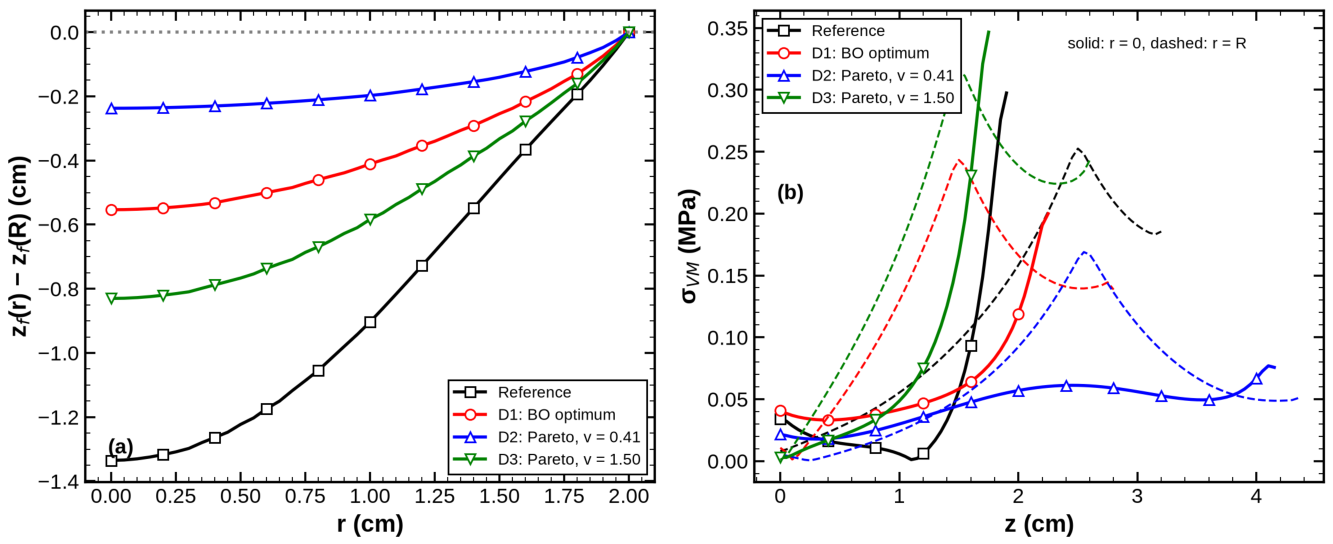

Table 1.
Physical properties of CdTe used in the simulations.
| Property | Value | Unit / source |
|---|---|---|
| Melting temperature, | 1092 (1365 K) | ∘C [5] |
| Latent heat of fusion, | 209.2 | kJ/kg [5] |
| Conductivity at : solid/liquid | 1.319 / 1.568 | W/(m K) [5] |
| Solid density, | 5854 | kg/m3 [35] |
| Young’s modulus / Poisson’s ratio | 37.99 GPa / 0.351 | [35,36] |
| Thermal expansion coefficient, | K−1 [37] |
Table 2.
Design variables and bounds; reference-design values are in brackets.
| Variable | Meaning | Range [reference] | Unit |
|---|---|---|---|
| G | Nominal axial furnace gradient | 0.75–4.0 [1.0] | ∘C/cm |
| v | Translation (growth) rate | 0–2.0 [1.0] | mm/h |
| Start of gradient zone (growth stage) | 1.5–4.0 [2.5] | cm | |
| Length of gradient zone | 1.5–4.0 [3.0] | cm | |
| Cold-zone undercooling | 1.0–4.0 [2.0] | ∘C | |
| R | Charge radius | 1.0–2.5 [2.0] | cm |
Table 3.
Surrogate accuracy: five-fold cross-validation (CV) on 400 runs and independent testing on 60 runs. Errors have the units of the corresponding output.
Table 3.
Surrogate accuracy: five-fold cross-validation (CV) on 400 runs and independent testing on 60 runs. Errors have the units of the corresponding output.
| Output | Model | |||||
|---|---|---|---|---|---|---|
| (cm) | GPR | 0.9953 | 0.0465 | 0.0289 | 0.9964 | 0.0395 |
| RF | 0.8790 | 0.2363 | 0.1687 | 0.9212 | 0.1860 | |
| GB | 0.9385 | 0.1685 | 0.1172 | 0.9667 | 0.1208 | |
| MLP | 0.9985 | 0.0264 | 0.0170 | 0.9990 | 0.0211 | |
| (MPa) | GPR | 0.9746 | 0.0240 | 0.0168 | 0.9771 | 0.0225 |
| RF | 0.8863 | 0.0509 | 0.0400 | 0.9249 | 0.0407 | |
| GB | 0.9358 | 0.0382 | 0.0300 | 0.9501 | 0.0332 | |
| MLP | 0.9410 | 0.0367 | 0.0259 | 0.9510 | 0.0329 | |
| (MPa) | GPR | 0.9830 | 0.0172 | 0.0130 | 0.9888 | 0.0141 |
| MLP | 0.9796 | 0.0189 | 0.0133 | 0.9914 | 0.0124 | |
| GB / RF | 0.929 / 0.884 | 0.035 / 0.045 | 0.027 / 0.035 | 0.941 / 0.913 | 0.032 / 0.039 | |
| (∘C/cm) | GPR | 0.9873 | 0.110 | 0.076 | 0.9925 | 0.080 |
| MLP | 0.9894 | 0.100 | 0.065 | 0.9932 | 0.076 | |
| GB / RF | 0.893 / 0.818 | 0.318 / 0.415 | 0.226 / 0.297 | 0.904 / 0.869 | 0.285 / 0.332 | |
| (cm) | GPR | 0.9978 | 0.0495 | 0.0303 | 0.9984 | 0.0419 |
| MLP | 0.9988 | 0.0360 | 0.0231 | 0.9996 | 0.0216 |
Table 4.
Selected designs at cm, recomputed with the solver ( cm). GPR predictions are in parentheses.
Table 4.
Selected designs at cm, recomputed with the solver ( cm). GPR predictions are in parentheses.
| Design | G | v | J | |||||||
|---|---|---|---|---|---|---|---|---|---|---|
| ∘C/cm | mm/h | cm | cm | ∘C | cm | MPa | MPa | cm | ||
| Reference | 1.00 | 1.00 | 2.50 | 3.00 | 2.00 | 0.339 | 0.282 | 1.91 | 6.30 | |
| D1 (BO) | 0.75 | 1.00 | 1.50 | 2.00 | 4.00 | 0.243 | 0.196 | 2.28 | 3.30 | |
| GPR+DE | 0.75 | 1.00 | 1.50 | 1.50 | 4.00 | 0.301 | 0.192 | 2.04 | 3.34 | |
| (prediction) | () | (0.291) | (0.202) | (3.28) | ||||||
| D2 (round 0) | 0.75 | 0.41 | 2.56 | 2.75 | 4.00 | 0.169 | 0.077 | 4.16 | 1.88 | |
| (prediction) | () | (0.196) | (0.101) | |||||||
| D3 (round 2) | 0.76 | 1.50 | 1.50 | 1.70 | 3.99 | 0.388 | 0.336 | 1.78 | 5.00 | |
| (prediction) | () | (0.399) | (0.341) |
Disclaimer/Publisher’s Note: The statements, opinions and data contained in all publications are solely those of the individual author(s) and contributor(s) and not of MDPI and/or the editor(s). MDPI and/or the editor(s) disclaim responsibility for any injury to people or property resulting from any ideas, methods, instructions or products referred to in the content. |
© 2026 by the authors. Licensee MDPI, Basel, Switzerland. This article is an open access article distributed under the terms and conditions of the Creative Commons Attribution (CC BY) license (http://creativecommons.org/licenses/by/4.0/).
Copyright: This open access article is published under a Creative Commons CC BY 4.0 license, which permit the free download, distribution, and reuse, provided that the author and preprint are cited in any reuse.