

Submitted:
14 November 2026
Posted:
17 November 2026
You are already at the latest version
Abstract
We prove that the \( h \)-polynomial of the antiprism triangulation of every simplicial complex with nonnegative \( h \)-vector has only real roots, as Athanasiadis, Brunink and Juhnke-Kubitzke conjectured. The key step is their conjecture that the \( h \)-polynomial of the antiprism triangulation of a simplex interlaces the theta polynomial of the next simplex. For the local \( h \)-polynomial we prove a convolution identity and reduce its conjectured real-rootedness to one interlacing relation of the same shape, which holds for \( n\le40 \).
Keywords:
antiprism triangulation
; real-rooted polynomials
; interlacing
MSC: Primary 05E45; 26C10; Secondary 05A15; 52B05
1. Introduction
Let be a finite simplicial complex of dimension with faces of dimension . Its h-polynomial is defined by
The h-vector is nonnegative for every Cohen–Macaulay complex, in particular for every triangulation of a ball or a sphere [16]. A recurring question in geometric combinatorics asks which subdivisions turn a nonnegative h-polynomial into a polynomial with only real roots. Brenti and Welker [11] proved that this happens for the barycentric subdivision : the polynomial is real-rooted whenever has nonnegative coefficients. Real-rootedness implies the log-concavity and unimodality of the coefficients.
The antiprism triangulation was introduced by Izmestiev and Joswig [13] in their study of branched coverings of manifolds, and appears in theoretical distributed computing as the chromatic subdivision1 [14]. Its vertices are the pointed faces of , with , and its faces are the sets with and whenever and [1,3]. Figure 1 shows the antiprism triangulation of a triangle. Athanasiadis, Brunink and Juhnke-Kubitzke [1] developed the combinatorics of and showed that it shares many properties of the barycentric subdivision, often in a harder form. Their main motivation was the following analogue of the theorem of Brenti and Welker.
Conjecture 1
([1] [Conjecture 1.1]). The polynomial is real-rooted for every simplicial complex Δ with nonnegative h-vector.
Write for the -dimensional simplex and for its boundary, and set
Athanasiadis, Brunink and Juhnke-Kubitzke proved that is real-rooted and interlaces [1] [Theorem 5.2]. Using the theory of uniform triangulations of Athanasiadis [2] [Theorem 1.2], they reduced Conjecture 1 to a single interlacing relation between two explicit sequences of polynomials.
Conjecture 2
([1] [Conjecture 5.3]). The polynomial interlaces for every .
They verified Conjecture 2 by computer for . Athanasiadis and Tzanaki [4] [Section 3] observed that it is the only missing part of the strong interlacing property of the antiprism triangulation, and Athanasiadis recorded Conjecture 1 again as open in [3] [Section 6]. We prove both conjectures.
Theorem 3.
Let Δ be an -dimensional simplicial complex with nonnegative h-vector. Then is real-rooted. Moreover, interlaces , which in turn interlaces .
Theorem 4.
For every the polynomial interlaces . Equivalently, the polynomial
interlaces . Moreover has degree , leading coefficient and only negative roots, so all its coefficients are positive.
Theorem 4 is Conjecture 2, and Theorem 3, which we derive from it, settles Conjecture 1. Together with the results of Athanasiadis and Tzanaki [4], which build on the work of Brändén and Solus [10], it gives real-rooted symmetric decompositions for antiprism triangulations of skeleta, and it implies that the -polynomial of the antiprism triangulation of any homology sphere is real-rooted (Section 6).
Corollary 1.
Let Δ be an -dimensional simplicial complex.
- (a)
- If Δ is Cohen–Macaulay, then the h-polynomial and the f-polynomial of are real-rooted; their coefficients are log-concave and unimodal.
- (b)
- If Δ is a homology sphere, then with real-rooted; in particular all are nonnegative and form a log-concave sequence.
- (c)
- If Δ is the -skeleton of an n-dimensional complex Γ with nonnegative h-vector, then has a nonnegative, real-rooted and interlacing symmetric decomposition with respect to n, and it interlaces .
Part (b) strengthens the -positivity proved by Athanasiadis [3] [Corollary 6.1], which confirmed Gal’s conjecture [12] for antiprism triangulations of homology spheres.2
The local h-polynomial is conjectured to be real-rooted as well [1] [Conjecture 5.8]. In Section 8 we express it through by a convolution in which every factor is real-rooted (Theorem 7), and we show that the part of the conjecture concerning , in a strong form that includes the interlacing of a whole local analogue of the sequence of [1], is equivalent to the relations and for all n (Theorem 8). The second relation has the shape of Theorem 4. Both relations hold for ; we do not know a proof.
The Idea of the Proof
Athanasiadis, Brunink and Juhnke-Kubitzke proved that is real-rooted by means of an interlacing sequence of polynomials whose partial sums are , with and . We show that the symmetric part of splits along the same partial sums,
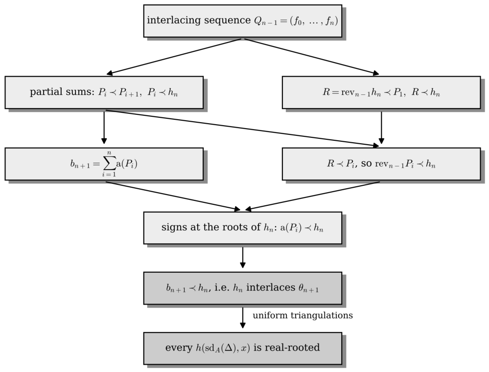
where . Each summand is interlaced against by a sign count at the roots of , because both and its reverse interlace . The second fact is the heart of the matter: it follows from the observation that the reverse of itself sits at the start of the interlacing chain . Figure 3 shows the structure of the argument. The passage from simplices to all complexes follows the method of Athanasiadis [2]; we give a complete proof, with a short “rotation lemma” in place of the general results on interlacing-preserving matrices that are used there.
Organization
Section 2 collects the facts about interlacing that we use, with proofs. Section 3 recalls the recurrence for and the interlacing sequence of [1]. Section 4 proves Theorem 4, and Section 5 proves Theorem 3. Section 6 derives the consequences, Section 7 gives examples and tables, Section 8 treats the local h-polynomial, and Section 9 describes the computer checks. Section 10 lists open problems.
2. Interlacing
All polynomials have real coefficients. A polynomial is real-rooted if all its complex roots are real. In this section every polynomial is nonzero, real-rooted and has a positive leading coefficient, unless stated otherwise. For such a polynomial f with roots , listed with multiplicity, put
For and a polynomial p of degree at most d we write .
Definition 1.
Let f have roots and g have roots . We say that finterlacesg, and write , if and
A sequence isinterlacingif for all .
Thus the largest root belongs to g, and a constant interlaces every polynomial of degree at most one. In particular for every f.3
Lemma 1.
if and only if for all .
Proof.
If , then on running t downwards from the roots are met in the order , so alternates between 1 and 0 (ties only shorten the steps). Conversely, assume the inequalities. Since , we get , that is, . Since , we get , that is, . Letting gives . □
Lemma 2.
- (a)
- If c is real-rooted with positive leading coefficient, then if and only if .
- (b)
- If or , and β is a root of g of multiplicity m, then β is a root of f of multiplicity at least .
- (c)
- (Weak transitivity.)If and , then is interlacing.
Proof. (a) and , so the differences in Lemma 1 agree. (b) Put and choose with no root of f or g in . Then . Both values of D lie in , or both lie in , so . (c) Put . For the difference is a sum of consecutive differences , hence it is nonnegative and bounded by the full sum . □
For g with distinct roots of multiplicities put and , so that has only simple roots. By Lemma 2, if (or ), then divides f, and (respectively ). This reduces most questions to the case of simple roots, where the following sign test applies.
Lemma 3
(Sign test). Let g have degree d and simple roots , and let f be a nonzero polynomial with positive leading coefficient.
- (i)
- if and only if and for .
- (ii)
- if and only if and for .
In both cases f is real-rooted.
Proof.
If (respectively ), then f has exactly (respectively k) roots larger than , unless ; this gives the signs. For the converse let and , so that divides f, and put . If is the r-th element of K in increasing order, then has sign , so is nonzero with sign in case (i) and in case (ii). Hence has a root in each of the open intervals between consecutive points , . In case (i), , and when the signs at the smallest point , , and at differ, which places the last root of below all these points. In case (ii) the sign at the largest point is negative and the sign at is positive, which places one root of above all points, and a possible further root lies below all points. So all roots of are real and located, and takes values in in case (i) and in in case (ii). Lemma 1 finishes the proof. (If , then f is a positive multiple of g or of with real, and both cases follow from Lemma 1.) □
Lemma 4
(Sums). Let .
- (a)
- If for all i, then .
- (b)
- If for all i, then .
- (c)
- If , then .
Proof.
For (a) and (b), divide all polynomials by and apply Lemma 3 to : the sign conditions and the conditions on the degree are preserved by positive linear combinations, since leading coefficients are positive and cannot cancel. (c) follows from (a) and (b) with and . □
Lemma 5
(Multiplication by x and reversal). Suppose that all roots of f and g are nonpositive.
- (a)
- if and only if .
Suppose moreover that all roots are negative.
- (b)
- If , then if and only if .
- (c)
- If , then if and only if .
Proof. (a) . For all counting functions vanish, and for the two conditions of Lemma 1 coincide. (b), (c) The roots of are the reciprocals of the roots of f, and reverses the order of . In (b) the relation reads , and taking reciprocals gives , which says . In (c) the chain becomes , which says . The converses follow by applying the same argument to the reversed polynomials. □
Lemma 6
- (a)
- The sequence is interlacing.
- (b)
- For , not all zero, is real-rooted, is interlaced by and interlaces .
- (c)
- .
Proof. (a) Let and . Every with interlaces every with , so by Lemma 4(a),(b), and then by Lemma 4(c). (b) for all i; apply Lemma 4(a),(b). (c) We first show, by induction on m, that for . For this is . For the sequence is interlacing, by Lemma 4, and has sum s; by induction . Also , since every term does. Adding preserves the relation by Lemma 4(b). Now by the claim, and ; add the two. □
3. The Antiprism Triangulation of a Simplex
3.1. The Recurrence
The polynomials satisfy and
[1] [Proposition 5.1]. The first values are
By induction on n, (1) shows that has nonnegative integer coefficients, , degree and leading coefficient n for : the term contributes the constant 1, the terms contribute , of degree k and with zero constant term, and only reaches degree , with coefficient . Since , the reverse has degree , constant term n and leading coefficient 1.4
3.2. The Symmetric Part
Every polynomial p of degree at most can be written uniquely as with and , namely
3.3. The Interlacing Sequence of Athanasiadis, Brunink and Juhnke-Kubitzke
For put
Then has nonnegative coefficients and degree with positive leading coefficient, and equals 1 if and 0 if . By (1) and Pascal’s rule,
Theorem 5
([1] [Theorem 5.2]). For every the sequence
is interlacing. In particular is real-rooted with negative roots, , and .
Proof.
We include the short proof of [1]. is interlacing. Let and assume that is interlacing. By (5), the first terms of are the partial sums of the reverse of , so they form an interlacing sequence by Lemma 6(a). By Lemma 2(c) it remains to show that and . By (6) the polynomial is the sum of the first terms of , so by Lemma 6(b). Applying Lemma 6(c) to , the sum is by (6) with in place of n, and by (5) and (6); hence . All polynomials involved have nonnegative coefficients, so their roots are nonpositive, and , , have nonzero constant terms, so their roots are negative. Now and , so is equivalent to by Lemma 2(a) and Lemma 5(c). Since , the relation is equivalent to by Lemma 5(a), and to by Lemma 5(b). This completes the induction. The last two terms of give , that is, , and the sum of the first n terms of interlaces its last term, that is, . □
4. Proof of Theorem 4
We prove that for every . For both polynomials equal 1, so let be fixed. Write , that is,
and let for . We record the properties we need.
- is interlacing (Theorem 5), all have nonnegative coefficients, for , and .
- , by (6) with in place of n.
- R has degree , leading coefficient 1 and negative roots, and .
Each has degree , nonnegative coefficients and . Hence has degree and leading coefficient 1. For a polynomial P of degree at most put
which is a polynomial because the numerator vanishes at .
Step 1: A Decomposition of
Lemma 7.
.
Proof.
Let , a linear map on polynomials of degree at most , and by (P3). For we have and therefore . Moreover and . Hence
On the other hand , so . Subtracting,
Dividing by and using (2) with in place of n gives the claim. □
Step 2: The Partial Sums
Lemma 8.
for , and for .
Proof.
For we have . By Lemma 4(a), for every . Taking and applying Lemma 4(c) gives . Summing over with Lemma 4(b) gives when , and then by Lemma 4(c). For the claim is . □
Step 3: The Reverse of Starts the Chain
Lemma 9.
for , and consequently for .
Proof.
First, . Indeed, by (P1), and this is equivalent to by Lemma 5(a), since both R and have nonnegative coefficients and real roots. Second, : by Lemma 4(a) the sum of interlaces , and is equivalent to by Lemma 5(a). By Lemma 8, and , so the sequence is interlacing by Lemma 2(c). In particular . Both polynomials have degree and negative roots, so Lemma 5(b) turns into . □
Step 4: The Sign Count
Lemma 10.
for .
Proof.
Let and , with simple roots , all negative. By Lemmas 8 and 9, and , so c divides and , and the quotients and satisfy and . By Lemma 3(i),
Since , the polynomial c divides and
At this gives
because the numerator is a nonpositive number minus a nonnegative number and the denominator is negative. Finally, has degree n and leading coefficient , so has degree and leading coefficient 1, and has degree d. Lemma 3(i) gives , hence . □
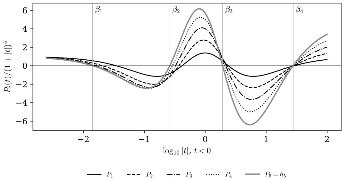
Figure 2.
The partial sums for , scaled by on the negative axis, against the roots of . All have the sign at , which is the sign condition of Lemma 3(i) behind .
Figure 2.
The partial sums for , scaled by on the negative axis, against the roots of . All have the sign at , which is the sign condition of Lemma 3(i) behind .
Step 5: Conclusion
By Lemmas 7 and 10 and Lemma 4(a),
Both polynomials have degree , so the largest root of is at most the largest root of , which is negative; thus all roots of are negative, and since its leading coefficient n is positive, all its coefficients are positive. By Lemma 5(a), is equivalent to . Since (Lemma 11(e) below), this is Conjecture 2 for , and Theorem 4 is proved.□
Example 1
Their sum is , as Lemma 7 asserts. The roots of are and . Each is positive at and negative at ; for instance and . So each interlaces , and so does , whose roots and satisfy . Multiplying by x, interlaces .
Remark 1.
The proof uses only Theorem 5 and the recurrence (1); it never refers to the combinatorics of . The polynomial is the part b of the symmetric decomposition, with respect to n, of the polynomial , so Lemma 7 says that the symmetric part of is assembled from the symmetric parts of the reversed partial sums . Figure 3 summarizes the argument.
Figure 3.
Structure of the proof of Theorems 4 and 3. Here means that f interlaces g.
5. All Simplicial Complexes
5.1. The Transformation of the H-Polynomial
For let , where is the number of -dimensional faces of that do not lie in , the interior faces; thus counts the empty face. The antiprism triangulation is compatible with restriction: for every face F of the faces of with carrier F are the interior faces of [1] [Section 4], [3] [Section 6]. Sorting the faces of by their carriers gives
where and E is the linear map with . This is the uniform structure studied by Athanasiadis [2]. For a polynomial of degree at most n put , so that for an -dimensional complex . For define
Since and has dimension , (7) and linearity give
The polynomials coincide with those of [2] [Theorem 4.1]. We use the reciprocity theorem for balls: if triangulates an -dimensional ball and counts its interior faces, then
Lemma 11.
For :
- (Lemma 11.)
- ;
- (b)
- for ;
- (c)
- ;
- (d)
- ;
- (e)
- , and hence .
Put . Summing (b) and using (a), (d), (e) gives the recurrence of [2] [Lemma 6.3],
Indeed, and .
5.2. The Rotation Lemma
Lemma 12.
Let and let be an interlacing sequence of nonzero polynomials with nonnegative coefficients. For put
Then is an interlacing sequence of polynomials with nonnegative coefficients.
Proof.
Note . Since interlaces every , it interlaces , so is real-rooted with nonpositive roots, and by Lemma 5(a) applied to . By Lemma 2(c) it suffices to show for . Fix k and put , which is nonzero because . Then
For we have , and also by Lemma 5(a). For we have , hence by Lemma 5(a) and by Lemma 2(a). Thus every summand of U is interlaced by and interlaces , so by Lemma 4. By Lemma 4(c), ; in particular is real-rooted, and its roots are nonpositive. Let . As , c divides U, hence also . If are the roots of , then
and by Lemma 3(ii) applied to . For the degrees: gives , and gives . Lemma 3(ii) yields , that is, . □
5.3. Proof of Theorem 3
For let . We show by induction on n that is an interlacing sequence of nonzero polynomials with nonnegative coefficients. For , Lemma 11(a),(c) give . Let and consider
Its first n terms form , which is interlacing with nonnegative coefficients by induction; has positive coefficients by Theorem 4. We have by Theorem 4. Further, by Lemma 11(c), and (Theorem 4) gives by Lemma 5(b), hence by Lemma 2(a). By Lemma 2(c), is interlacing. Lemma 12 applied to produces with for by (10), so is interlacing with nonnegative coefficients.
Now let be -dimensional with nonnegative h-vector. By (8), is a nonnegative combination of , not identically zero because . Lemma 6(b) shows that it is real-rooted, interlaced by , and interlaces . This proves Theorem 3.□
The same argument proves that is real-rooted for every polynomial h of degree at most n with nonnegative coefficients, whether or not it is the h-polynomial of a complex.
6. Consequences
6.1. Cohen–Macaulay Complexes
If is Cohen–Macaulay over some field, its h-vector is nonnegative [16] [Chapter II], so is real-rooted with nonpositive roots. The f-polynomial is then real-rooted as well: each linear factor of h with becomes . By Newton’s inequalities the coefficients of both polynomials are log-concave with no internal zeros, hence unimodal. This proves Corollary 1(a) and strengthens the unimodality of the h-vector of proved in [1] [Theorem 1.3].
6.2. Homology Spheres
If is a homology sphere, then so is , and is symmetric of degree n by the Dehn–Sommerville equations. A symmetric real-rooted polynomial h with nonnegative coefficients has its roots in pairs with , together with the root ; each pair contributes
Hence with , and substituting gives
which is real-rooted with nonpositive roots. This proves Corollary 1(b).
6.3. The Strong Interlacing Property
In the language of Athanasiadis and Tzanaki [4] [Definition 3.2], a uniform triangulation has the strong interlacing property if is real-rooted for and is zero or a real-rooted polynomial of degree with nonnegative coefficients interlaced by for . For the antiprism triangulation, the first condition is Theorem 5, and the second is Theorem 4 with Lemma 11(e). Thus the antiprism triangulation has the strong interlacing property for every n, which was the open part of [1] [Section 5] recorded in [4] [Section 3]. The main results of [4] [Theorems 4.1 and 6.1] therefore apply. In particular, if is an n-dimensional complex with nonnegative h-vector and is its -skeleton, then has a nonnegative, real-rooted and interlacing symmetric decomposition with respect to n, and it interlaces [4] [Theorem 6.1]. This is Corollary 1(c).
6.4. The Boundary of the Simplex
The sequence of Section 5 is interlacing, and its first term is . By Lemma 6(b), interlaces the sum of its first n terms, which is by Lemma 11(d),(e), and the sum of all its terms, which is .
Corollary 2.
For every the polynomial interlaces , and , and interlaces .
The relation is part of [1] [Theorem 5.2]; the relations with and are new.
7. Examples and Tables
Example 2
Example 3
(Two triangles). Let Δ consist of two triangles sharing an edge, a 2-ball with and . Then , with roots .
Example 4
(Three-spheres). For the boundary of the 4-simplex, and , with . For the boundary of the 4-dimensional cross-polytope, and , with . Both γ-polynomials have positive discriminant, as Corollary 1(b) predicts.
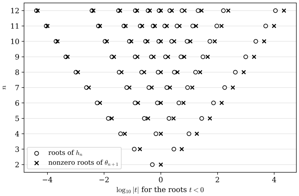
Figure 4.
Roots of and nonzero roots of on a logarithmic scale. The alternation in each row is the interlacing of Theorem 4.
Figure 4.
Roots of and nonzero roots of on a logarithmic scale. The alternation in each row is the interlacing of Theorem 4.
Two features of Table 3 deserve comment. Since is symmetric, its roots come in reciprocal pairs, and for odd n it has odd degree and therefore the root . In the table the largest root of approaches 0 and the smallest one decreases quickly; by Theorem 3 the roots of every with interlace those of .
8. The Local H-Polynomial of the Simplex
The restriction of to a face of with i vertices is the antiprism triangulation of that face. Hence the local h-polynomial of Stanley [15] satisfies
The first values are , , , and . By [15] [Theorem 3.3] the polynomial is symmetric, , and for it has degree , zero constant term and leading coefficient n.5 Write and .
Conjecture 6
([1] [Conjecture 5.8]). For every n the polynomial is real-rooted and interlaces , and is real-rooted and interlaces .
Theorem 4 says that interlaces . This section shows that the first half of Conjecture 6 is equivalent to an interlacing relation of the same shape, , taken together with , and gives two identities that express through .
8.1. Generating Functions
Put
Proposition 1.
, and
Consequently , where denotes a Stirling number of the second kind.
Proof.
The recurrence [1] [(18)], , is the coefficientwise form of Proposition 1. Its kernels have non-real roots for . Differentiating instead gives a convolution in which every factor is real-rooted. For put
By Theorem 5 and Lemma 5(a) we have , so is real-rooted by Lemma 4(c); it is symmetric with center of symmetry .
Theorem 7.
For every ,
Proof.
Differentiating gives
By Proposition 1, . Also , since the difference of the two sides is . Hence with
Comparing coefficients of in gives the first identity. Since , we get , which gives the second. □
In other words, has the exponential coefficients : the local h-polynomials are the moments whose cumulants are . For example, , with and . Every summand of Theorem 7 is real-rooted whenever is, but for none of the nonzero summands with interlaces , so the identity does not by itself give real-rootedness.
8.2. A Decomposition Along an Interlacing Chain
For put
the local analogue of the polynomials of Section 3. Then by (11), , and Pascal’s rule gives for . Fix and put
All have degree at most . As in Section 4, for a polynomial P of degree at most .
Proposition 2.
For we have , , and
Proof.
Iterating Pascal’s rule along the antidiagonal gives for ; the case is the first identity. Summing over r gives , and the same iteration at level gives , which is the second identity.
Let and , a symmetric polynomial of degree , so that and . With from (2), the polynomial satisfies . On the other hand for every j, so
because . Since , dividing by gives . □
By Theorem 4 the first summand interlaces , and since , Lemma 10 shows that interlaces . Thus , which by Lemma 5(a) is the relation , would follow from . This is where the method of Section 4 stops. The tail sums vanish at 0; for they are interlaced by rather than interlacing it, and none of the real-rooted polynomials interlaces , while .
8.3. A Reduction of Conjecture ??
For consider the sequence
the local analogue of the sequence of Theorem 5. For all its terms are nonzero.
Theorem 8.
The sequence is interlacing. For , if is interlacing, then is interlacing if and only if
Consequently is interlacing for every if and only if and for every . In that case the first half of Conjecture 6 holds, since for there is nothing to prove, and every polynomial is real-rooted.
Proof.
The roots of the terms of are , 0, 0 and , and the relations required by the definition are immediate. Let and assume that , in the notation of Proposition 2, is interlacing. By the proof of that proposition the first terms of are , the partial sums of taken from the end, so they form an interlacing sequence by Lemma 6(a). The two displayed relations are relations between terms of , so they are necessary. Conversely, they provide the last consecutive relation and the relation between the first and the last term, and Lemma 2(c) shows that is interlacing. The remaining statements follow by induction on n; every with is a term of . □
The proof of Theorem 5 obtained the analogous two relations for from the recurrence (1). For they carry the local information, and they are the whole difficulty. The second relation has the shape of Theorem 4, with in place of ; both and are x times a symmetric polynomial of degree .
Proposition 3.
For ,
where with . Consequently is interlacing for , and the statements of Conjecture 6 and of [1] [Conjecture 5.6] hold for .
Proof.
The four relations are finite statements about explicit integer polynomials. They were decided by exact Sturm sequences, as described in Section 9. The second assertion follows from Theorem 8. □
9. Computer Verification
Every statement of the paper is proved in the text. We nevertheless checked the finite content by two independent programs, archived in the public repository https://github.com/creelie/d-dome-enrique.
Lean 4
A Lean 4 project with Mathlib contains a kernel-checked proof of the general identity behind Lemma 7, stated for an arbitrary additive group with two additive maps, and of the sign transfer inequality of Lemma 10: if , , and , then . It also verifies, by evaluation in the kernel, the recurrence (1) against the table of [1], and the identities (P2), (P3), and Lemma 7 with exact integer arithmetic for . The only axioms used are the standard ones of Lean (propext, Classical.choice, Quot.sound).
Julia
A Julia program computes , , and in exact integer arithmetic and decides each interlacing relation by Sturm sequences after removing common factors, without floating point. For every it confirms (6), Lemma 7, the degrees and positivity of , all interlacing relations of , and the relations of Lemmas 8–10 and Theorem 4, 2127 checks in total. Deliberately wrong inputs are rejected.
Two further programs, with the same exact Sturm test, check Section 8. For every the first confirms that is symmetric with zero constant term, its expansion in the numbers , the two convolution identities of Theorem 7, the decomposition of in Proposition 2, and the relations , and . For it also checks directly that is interlacing, and for it checks every pair in ; these direct checks are redundant by Theorem 8. It makes 1066 checks. The second program confirms for and, for , that no with interlaces while , which is the failure of termwise interlacing discussed after Proposition 2; it makes 114 checks.
10. Open Problems
By Theorem 8, the first half of Conjecture 6, together with the interlacing of all sequences , comes down to one question.
Question 9.
Does interlace , and does interlace , for every ?
Proposition 2 shows that the method of Section 4 needs one more ingredient here: a chain that controls the tail sums and their reversals, in the way that controls the partial sums in Lemma 9. Another possible route starts from the identity of [1] [Proposition 5.9], where is the mth derangement polynomial: by Theorem 4 every is real-rooted, so each summand is real-rooted, and the question is whether the summands have a common interlacer. More generally, Athanasiadis asked whether is real-rooted for every triangulation of a simplex [3] [Question 6.3]; the case is Conjecture 6.
A second question is whether the interlacing in Theorem 4 is strict, that is, whether and have no common root; in all computed cases they have none.
Author Contributions
Deep Bhattacharjee is the sole author. He chose the problem, proved the results, wrote the paper, drew the figures, and wrote the Lean 4 and Julia programs that check the finite statements.
Funding
No funding of any kind was received for this work.
Ethics approval
Not applicable. The work involves no human participants, animals or personal data.
Data and code availability
No data were generated. The Lean 4 project and the Julia programs that recompute every numerical statement of the paper are available at https://github.com/creelie/d-dome-enrique. The Lean files are checked by the kernel, with no unproved statement and no axiom beyond the standard ones.
Competing interests
The author declares no competing interests.
Open Gluon and Anaxia
Two tools built by the author organised this project. Open Gluon is a workspace that keeps pinned copies of the mathematical libraries, the source record of the project and its checks in one reproducible place. Anaxia, the engine of the eBLLM project, stores each construction as a route with its input, its output, the obligations that must be discharged and a test that makes the route fail when an obligation is skipped, and it certifies finite statements in exact integer and rational arithmetic. It was used here to keep the polynomial data of Section 3, Section 4, Section 5, Section 6 and Section 7 and their checks in one record. Every statement of this paper is proved in the text.
References
- Athanasiadis, Christos A.; Brunink, Jan-Marten; Juhnke-Kubitzke, Martina. Combinatorics of antiprism triangulations. Discret. Comput. Geom. 2022, 68(no. 1), 72–106. [Google Scholar] [CrossRef]
- Athanasiadis, Christos A. Face numbers of uniform triangulations of simplicial complexes. Int. Math. Res. Not. 2022, no. 20, 15756–15787. [Google Scholar] [CrossRef]
- Athanasiadis, Christos A. Triangulations of simplicial complexes and theta polynomials. Tohoku Math. J. 78 (2026)(no. 3), 423–441. [CrossRef]
- Athanasiadis, Christos A.; Tzanaki, Eleni. Symmetric decompositions, triangulations and real-rootedness. Mathematika 2021, 67(no. 4), 840–859. [Google Scholar] [CrossRef]
- Bhattacharjee, Deep. Establishing equivariant class [O] for hyperbolic groups. Asian Res. J. Math. 2022, 18(no. 11), 362–369. [Google Scholar] [CrossRef]
- Bhattacharjee, Deep. Non-commutativity over canonical suspension η for genus g≥1 in hypercomplex structures for potential ρϕ. Asian Res. J. Math. 2022, 18(no. 11), 332–341. [Google Scholar] [CrossRef]
- Bhattacharjee, Deep; Bhattacharya, Ushashi. Iterated nerve complexes for k-fold sensor coverage. Preprints.org 2026. [Google Scholar] [CrossRef]
- Brändén, Petter. On linear transformations preserving the Pólya frequency property. Trans. Am. Math. Soc. 2006, 358(no. 8), 3697–3716. [Google Scholar] [CrossRef]
- Brändén, Petter. Unimodality, log-concavity, real-rootedness and beyond. In Handbook of Enumerative Combinatorics; CRC Press: Boca Raton, 2015; pp. 461–508. [Google Scholar] [CrossRef]
- Brändén, Petter; Solus, Liam. Symmetric decompositions and real-rootedness. Int. Math. Res. Not. 2021, no. 10, 7764–7798. [Google Scholar] [CrossRef]
- Brenti, Francesco; Welker, Volkmar. f-vectors of barycentric subdivisions. Math. Z. 2008, 259(no. 4), 849–865. [Google Scholar] [CrossRef]
- Gal, Światosław R. Real root conjecture fails for five- and higher-dimensional spheres. Discret. Comput. Geom. 2005, 34(no. 2), 269–284. [Google Scholar] [CrossRef]
- Izmestiev, Ivan; Joswig, Michael. Branched coverings, triangulations, and 3-manifolds. Adv. Geom. 2003, 3(no. 2), 191–225. [Google Scholar] [CrossRef]
- Kozlov, Dmitry N. Chromatic subdivision of a simplicial complex. Homol. Homotopy Appl. 2012, 14(no. 2), 197–209. [Google Scholar] [CrossRef]
- Stanley, Richard P. Subdivisions and local h-vectors. J. Am. Math. Soc. 1992, 5(no. 4), 805–851. [Google Scholar] [CrossRef]
- Richard P. Stanley, Combinatorics and Commutative Algebra. In Progress in Mathematics, second ed.; Birkhäuser, Boston, 1996; vol. 41.
- Wagner, David G. Total positivity of Hadamard products. J. Math. Anal. Appl. 1992, 163(no. 2), 459–483. [Google Scholar] [CrossRef]
| 1 | The chromatic subdivision of a simplex describes the protocol complex of one round of an immediate snapshot in a shared-memory system; Kozlov [14] gives a combinatorial treatment and shows that it is a subdivision. |
| 2 | Gal [12] showed that the h-polynomial of a flag sphere need not be real-rooted in dimension five and higher, so real-rootedness is a special feature of the triangulations considered here and not a general property of flag spheres. |
| 3 | |
| 4 | The coefficients of have several combinatorial interpretations; for instance, the coefficient of is times the number of permutations of with excedance set [1] [Proposition 5.1]. We shall not need them. |
| 5 | Athanasiadis, Brunink and Juhnke-Kubitzke proved that is -positive [1] [Proposition 5.9] and gave several combinatorial interpretations of its coefficients [1] [Proposition 5.7]; for instance, the coefficient of counts ordered set partitions of with an even number of blocks such that has k elements. |
Figure 1.
The antiprism triangulation of the triangle with vertices . The three interior vertices are the three pointed faces of the whole triangle, each edge carries two vertices, the pointed edges, and the complex has 12 vertices and 13 triangles, the number of ordered set partitions of . Its h-polynomial is .
Figure 1.
The antiprism triangulation of the triangle with vertices . The three interior vertices are the three pointed faces of the whole triangle, each edge carries two vertices, the pointed edges, and the complex has 12 vertices and 13 triangles, the number of ordered set partitions of . Its h-polynomial is .
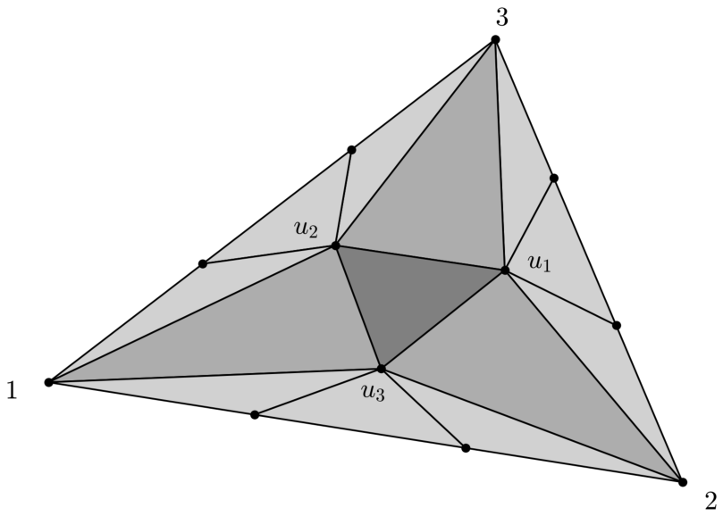

Table 1.
The polynomials and , listed by their coefficients in increasing degree.
| n | ||
|---|---|---|
| 2 | 1, 2 | 1 |
| 3 | 1, 9, 3 | 2, 2 |
| 4 | 1, 28, 42, 4 | 3, 17, 3 |
| 5 | 1, 75, 310, 150, 5 | 4, 79, 79, 4 |
| 6 | 1, 186, 1725, 2300, 465, 6 | 5, 284, 859, 284, 5 |
| 7 | 1, 441, 8211, 23625, 13685, 1323, 7 | 6, 888, 6362, 6362, 888, 6 |
| 8 | 1, 1016, 35476, 193256, 241570, 70952, 3556, 8 | 7, 2547, 38023, 86337, 38023, 2547, 7 |
| 9 | 1, 2295, 143676, 1367100, 3179106, 2050650, 335244, 9180, 9 | 8, 6893, 198461, 882011, 882011, 198461, 6893, 8 |
Table 2.
The polynomials for , by their coefficients in increasing degree. Each row is an interlacing sequence; the row sums are .
Table 2.
The polynomials for , by their coefficients in increasing degree. Each row is an interlacing sequence; the row sums are .
| n | |
|---|---|
| 1 | , |
| 2 | , , |
| 3 | , , , |
| 4 | , , , , |
Table 3.
Roots of and of (six significant digits). The roots of the two polynomials alternate, the smallest belonging to , as Theorem 4 asserts.
Table 3.
Roots of and of (six significant digits). The roots of the two polynomials alternate, the smallest belonging to , as Theorem 4 asserts.
| n | roots of | roots of |
|---|---|---|
| 2 | ||
| 3 | , | , |
| 4 | , , | , , |
| 5 | , , , | , , , |
| 6 | , , , , | , , , , |
| 7 | , , , , , | , , , , , |
Disclaimer/Publisher’s Note: The statements, opinions and data contained in all publications are solely those of the individual author(s) and contributor(s) and not of MDPI and/or the editor(s). MDPI and/or the editor(s) disclaim responsibility for any injury to people or property resulting from any ideas, methods, instructions or products referred to in the content. |
© 2026 by the authors. Licensee MDPI, Basel, Switzerland. This article is an open access article distributed under the terms and conditions of the Creative Commons Attribution (CC BY) license (http://creativecommons.org/licenses/by/4.0/).
Copyright: This open access article is published under a Creative Commons CC BY 4.0 license, which permit the free download, distribution, and reuse, provided that the author and preprint are cited in any reuse.