
Submitted:
16 November 2026
Posted:
17 November 2026
You are already at the latest version
Abstract
Acid-catalyzed degradation limits the stability of many organic molecules, and its study often requires advanced instruments. This study shows how cyclic voltammetry, UV-vis spectroscopy, and density functional theory (DFT) calculations, available in most laboratories, can be combined to study such reactions, using murexide as a model system. The degradation of murexide, measured by the decrease in its cyclic voltammetric peak current, followed pseudo-first-order kinetics. The apparent rate constants were 0.0058, 0.0119, and 0.0343 min⁻¹, with half-lives of 119, 58, and 20 min at pH 4.9, 3.0, and 2.0, respectively. The UV-vis rate constant at pH 4.9 agreed with the electrochemical value. The large peak separation (730–742 mV) indicated slow electron transfer at the Pt electrode, with a transfer coefficient (α) of 0.32 and a heterogeneous electron transfer rate constant (k⁰) of (5.2 ± 0.2) × 10⁻4 cm s⁻¹. DFT calculations showed that protonation at the C5 carbon (calculated pKa ≈ 3.1) opens a low-energy hydrolysis pathway to alloxan and uramil. TDDFT analysis showed that the loss of the absorption at 510 nm is due to dis-ruption of the C5–N–C5 conjugation. This combined approach provides an accessible framework for studying acid-catalyzed degradation in research and teaching settings.
Keywords:
murexide
; cyclic voltammetry
; heterogeneous electron transfer rate constant
; diffusion coefficient
; transfer coefficient
; degradation kinetics
; acid-catalyzed degradation
; pKa calculations
; DFT
; TDDFT
1. Introduction
Acid-catalyzed degradation reactions are important in many fields. They determine the shelf life of pharmaceuticals [1,2], the stability of dyes, indicators, and food colorants [3,4], the performance of organic electrolytes in redox flow batteries [5,6], and the environmental fate of organic pollutants [7,8]. In each case, a reliable description of the reaction requires both its rate under relevant conditions and an understanding of the mechanism, including which protonation step initiates degradation. These questions are often addressed with specialized and expensive techniques such as stopped-flow spectroscopy, HPLC-MS, or in situ NMR [9,10], which are not available in every laboratory or teaching setting.
Electrochemical workstations, UV-vis spectrophotometers, and computers capable of running density functional theory (DFT) calculations are present in most chemistry teaching and research laboratories [11,12,13,14]. Together, these tools can provide rate constants, electron-transfer parameters, and an atomic-level picture of the most favorable reaction pathway. A clear, well-tested approach combining these techniques would be useful for both routine stability studies and training students to connect experimental observations with mechanistic interpretation. Murexide (ammonium purpurate) is well suited to develop such an approach. It is a classical dye that is still used as a metallochromic indicator for Ca2+ and other metal ions [15,16,17,18]. Its degradation was previously studied from an educational perspective at pH 5 to 9 [19], but its behavior in more acidic media has not been examined. Murexide is electrochemically active [20] and strongly absorbs visible light, so its decomposition can be followed by both cyclic voltammetry and UV-vis spectroscopy. Its degradation in acid occurs over minutes to hours, which makes the kinetics easy to observe with standard equipment. Its small molecular size also keeps the computational cost of DFT and time-dependent DFT (TDDFT) calculations low, so the calculations can be run on personal computers available in undergraduate teaching laboratories.
In this work, we studied the acid-catalyzed degradation of murexide at pH 4.9, 3.0, and 2.0 using cyclic voltammetry and UV-vis spectroscopy. We calculated the electron transfer kinetics of murexide with the Klingler–Kochi and Gileadi methods and used DFT and TDDFT calculations to identify the protonation site that drives hydrolysis and to explain the loss of the visible absorption. The degradation follows pseudo-first-order kinetics, and the rate increases about sixfold from pH 4.9 to pH 2.0. The calculations show that protonation at C5, with a calculated pKa of about 3.1, opens a low-energy hydrolysis pathway to alloxan and uramil [21,22]. The large peak separation indicates slow electron transfer at Pt, with k0 ≈ 1.4 × 10⁻³ cm s-1. Together, these results give a consistent molecular picture of murexide degradation and present murexide as an accessible model system for connecting solution kinetics, electrode kinetics, and quantum-chemical calculations.
2. Materials and Methods
2.1. Experimental Methods
2.1.1. Instrumentation
Cyclic voltammetry of Murexide was carried out using a CHI-760D Electrochemical Workstation, and UV-Visible spectroscopy was carried out using SHIMADZU-1800. The pH measurement was conducted by pH-meter of model 3510 of JENWAY. Voltammetry study of degradation of murexide was carried in conventional three electrode set up. All the experiments were carried out at room temperature. The working electrode was a platinum disk electrode (CHI 102, surface area = 0.0314 cm2), the counter electrode was a Pt wire, and the reference electrode was a saturated calomel electrode (SCE, CHI 150), all from CH Instruments Inc. (Austin, TX, USA). All three electrodes were immersed in the aqueous solution of murexide contained in a glass beaker with a fine-porosity tip. The working electrode was carefully polished before each experiment using an alumina slurry to remove any adsorbates. Other details of the reagents, chemicals, and solution preparation are given in Section S1 of the Supplementary Information.
2.1.2. Electrochemical Methods
All the experiments were performed at scan rates ranging from 0.1 to 0.5 V s−1, at room temperature. The degradation, which is proceeded by photon radiation (i.e., sunlight), requires that the murexide be cooled down before taking its voltammogram. Cathodic peak potential (Epc), anodic peak potential (Epa), cathodic peak current (Ipc), anodic peak current (Ipa), and half-peak potential (Ep/2) were obtained directly from CHI 760D software. In those CVs in which these parameters were not shown, they were taken manually from the CV curve using baselines as proposed by Nicholson and Shain. In this case, 50% of the peak current was evaluated, and with the help of the baseline, across the potential axis, Ep/2 was noted from the corresponding point on the curve [23]. Peak-to-peak separation was obtained from the difference between anodic and cathodic peak potentials (ΔE = Epa – Epc). Half-wave potential was also obtained from the average of the anodic and cathodic peak potentials using the formula E(1/2) = (Epa + Epc)/2. Peak current ratios were obtained by dividing the cathodic peak current by the anodic peak current, Ipc/Ipa.
2.2. Computational Methods
All DFT calculations were carried out using Gaussian 16 [24] with the B3LYP hybrid functional [25] and Grimme’s D3 dispersion correction [26]. Geometry optimizations and frequency calculations were performed with the 6-31G(d,p) basis set, and the absence of imaginary frequencies confirmed that all optimized structures are minima. Solvent effects of water were included with the SMD implicit solvation model [5]. This combination of functional and basis set has previously reproduced experimental pKa values and reduction potentials [27,28]. For the TD-DFT calculations, the B3LYP-D3/6-31G(d,p) optimized geometries were used, and excited-state calculations (TD-DFT) were carried out at the B3LYP/6-311++G(2d,p) level in water (SMD) and have been tested previously to reproduce experimental values for absorption maxima [29].
The pKa value of the protonated species was calculated using the methodology described in our previous studies [27,28]. The pKa values were calculated from the reaction free energy of [MP-H]0 → [MP]− + H+. The solvation free energy of the proton was taken from previously computed values, G°solv(H+) = −265.9 kcal/mol [30].
3. Results
In the following sections, we first discuss the electrode kinetics of murexide oxidation, then its degradation studied experimentally using cyclic voltammetry and UV-visible spectroscopy, and finally the degradation mechanism obtained from DFT and TDDFT calculations.
3.1. Electrode Kinetics
Cyclic voltammetric studies were carried out on a 5 mM murexide solution (pH 4.9) at scan rates ranging from 0.1 to 0.5 V s−1, as presented in Figure 1a, and all basic and derived data are presented in Tables S1 and S2 of the Supplementary Information, respectively. Voltammograms recorded at different scan rates provide first-hand information on whether a system is diffusion- or kinetically controlled, and whether it is reversible, quasi-reversible, or irreversible. The cyclic voltammograms in Figure 1a show a cathodic peak at approximately 0.26 V, while an anodic peak is observed around 1.0 V vs SCE, followed by a sharp increase in current at higher potentials. Both anodic and cathodic peak-current magnitudes increase with scan rate. The anodic peak current increases from 23 to 68 µA, while the cathodic peak-current magnitude increases from 16.2 to 55.2 µA. The anodic peak potential shifts slightly from 996 to 1002 mV, whereas the cathodic peak potential shifts from 266 to 260 mV. Consequently, the peak-potential separation increases from 730 to 742 mV, far larger than the approximately 59 mV expected for an ideal reversible one-electron process at 25 °C. The estimated formal potential remains relatively stable at approximately 631–633 mV. Meanwhile, the cathodic-to-anodic peak-current ratio increases from 0.70 to approximately 0.81, suggesting that the two peak currents do not increase proportionally across the scan-rate range (Tables S1–S2). The broad anodic peak and the large peak separation suggest a complex redox process that may involve coupled chemical reactions rather than a simple, fully reversible electron transfer.
The next test is whether the reaction is diffusion-controlled or kinetically controlled. The most commonly used test is a plot of peak current versus the square root of scan rate (R2 = 0.997, Figure S1a). Rarely, peak current versus scan rate (R2 = 0.989, Figure S1b) is used to check adsorption-controlled electron transfer. The decision between diffusion control and adsorption control is based on the R2 value. Here, R2 values are close, making it difficult to discern the controlling process. A more robust test is the plot of log peak current versus log scan rate, where the slope distinguishes diffusion from adsorption control. A slope of 0.5 corresponds to a diffusion-controlled process, while a slope of 1.0 corresponds to an adsorption-controlled process. The anodic peak current yielded a slope of 0.665 (R2 = 0.997, Figure 1b), which lies between these limits but closer to 0.5. This suggests that the electrode process is mainly diffusion-controlled, with some contribution from adsorption of murexide or its oxidation products on the Pt surface.
3.1.1. Transfer Coefficient and Diffusion Coefficient
After basic analysis of the voltammograms, the heterogeneous electron-transfer rate constant (k0) is determined. k0 is one of the most important parameters because it provides insight into electron-transfer kinetics at the electrode–solution interface. Calculating k0 first requires the transfer coefficient (α) and the diffusion coefficient (D). These parameters, together with the basic voltammetric parameters, are then used to determine k0. The transfer coefficient was determined using Eqn. 1 [31].
where Ep and Ep/2 are the peak and half-peak potentials (mV), respectively, and n is the number of electrons transferred (n = 1). Ep ─ Ep/2 increased slightly with scan rate, from 147.2 to 152.3 mV between 0.1 and 0.5 V s−1 (Table S2). The corresponding αn values remain constant at 0.33. The nearly constant αn across the scan-rate range indicates that the transfer coefficient is largely independent of scan rate under these conditions. The transfer coefficient can also be determined from the Tafel equation (Eqn. S1, see Supporting Information), but this approach is complicated by the difficulty of defining the Tafel region [32,33].
Ep ─ Ep/2 = 48/(αn)
The next parameter is the diffusion coefficient (D0). Because the process is quasi- or irreversible, D0 was calculated using the modified Randles–Ševčík equation, eqn. 2 [34,35,36].
Here, Ip is the peak current (A), A is the area of the working electrode (0.0314 cm2), C is the concentration (mol cm−3), n is the number of electrons involved (which is 1 here), α is the transfer coefficient obtained from Eqn. 1 (0.32), υ is the scan rate (V s−1), and D0 is the diffusion coefficient (cm2 s−1). The values calculated from the cathodic peak currents using Eqn. 2 are presented in Table 1. These values average 6.98 × 10⁻⁶ cm2 s−1, ranging from 3.87 × 10⁻⁶ cm2 s−1 at 0.1 V s−1 to 9.53 × 10⁻⁶ cm2 s−1 at 0.5 V s−1. D0 can also be determined from the slope of Ip versus υ1/2 (Figure S1a) using eqn. 3:
This method gives a value of 5.83 × 10⁻⁶ cm2 s−1. The slope method is less affected by constant background contributions, such as capacitive current, which appear in the intercept rather than the slope. The increase in D0 with scan rate and the nonzero intercept are consistent with the adsorption contribution indicated by the log–log analysis in Figure 1b.
3.1.2. Heterogeneous Electron Transfer Rate Constant (k0)
The heterogeneous electron transfer rate constant (k0) is the key kinetic parameter of the electrochemical system. Three methods are commonly used to calculate k0. The most widely used is the Nicholson and Shain method [7,37,38], which estimates k0 from the change in peak separation (ΔEp) with scan rate through a dimensionless kinetic parameter, ψ. This method is mostly limited to reversible and quasi-reversible systems, and ψ is not available or not reliable above a peak separation of about 200 mV [39,40]. For murexide, the peak separation is much wider (730–742 mV, Table S2), indicating that heterogeneous electron transfer is irreversible. We therefore used the Klingler–Kochi [14] and Gileadi [19,26] methods, which remain reliable for irreversible systems or when the reverse peak becomes weak at higher scan rates.
The Klingler–Kochi method [41] also relies on ΔEp but additionally includes the transfer coefficient (α), and calculates k0 directly at each scan rate:
k0 = 2.18(αnD0Fυ/RT)1/2 e–[α2nFΔEp/RT]
For each scan rate, ΔEp was obtained as Epa − Epc from the cyclic voltammograms (Table S2). These values were substituted into Eq. 4 with α = 0.32 (from Eq. 2), n = 1, D0 = 5.83 × 10⁻⁶ cm2 s−1 and F/RT = 38.94 V−1 (T = 298 K), and the resulting k0 values were averaged. k0 increased from 3.2 × 10⁻⁴ cm s−1 at 0.1 V s−1 to 6.8 × 10⁻³ cm s−1 at 0.5 V s−1, giving an average of (5.2 ± 0.2) × 10−4 cm s−1 (Table 2).
To compare with the Klingler–Kochi result, k0 was also estimated using the Gileadi method [35,38,42], which relies on the shift in peak potential rather than ΔEp. In this method, Ep is plotted against log υ. At low scan rates, the electron transfer is quasi-reversible, and Ep shifts only slightly with scan rate. Above a critical scan rate (υc), the process becomes irreversible, and Ep shifts more steeply. The two linear regions intersect at υc, which is then used in Eq. (5) together with α and D0 to calculate k0.
where υc is the critical scan rate at which the process changes from quasi-reversible to irreversible. We obtained υc from the intersection of the two linear regions in the plot of Ep versus log υ (Figure 2), giving υc = 0.301 V s−1. Using α = 0.32 and D0 = 5.83 × 10⁻⁵ cm2 s−1 and n = 1, eqn. 5 gives k0 = 7.21 × 10⁻³ cm s−1. The main limitation of this method is that υc must be located accurately. Here, Ep shifts by only 6 mV over the full scan-rate range (996–1002 mV), close to the measurement resolution, so the breakpoint and υc are poorly defined. We therefore treat the Gileadi value as an upper estimate.
logk0 = – 0.48α + 0.52 + log (αnD0Fυc /2.303RT)1/2
The Klingler–Kochi value is about an order of magnitude lower than the Gileadi estimate and is consistent with the large ΔEp, indicating slow electron transfer of murexide at Pt. A similar difference between the k0 values obtained from these two methods has been reported previously [35,37,38]. The increase of k0 with scan rate, together with the nearly constant ΔEp, suggests that a following chemical step contributes to the response, in line with the degradation observed in the kinetic measurements. The k0 values are therefore reported as apparent rate constants.
3.2. Acid-Catalyzed Murexide Degradation
The degradation of murexide was followed by cyclic voltammetry in three acidic media (pH 4.9, 3.0, and 2.0) by recording the oxidation peak current (Ip) of freshly prepared solutions over time under sunlight, and the resulting cyclic voltammograms are presented in Figure S3a–c. At all three pH values, Ip decreased steadily with time while the peak potentials remained nearly unchanged, indicating a loss of electroactive murexide rather than a change in its redox behavior. The rate of this decrease depended strongly on acidity. In acetate buffer at pH 4.9, Ip fell from 37 to 29 µA in the first 30 min and reached 9 µA after 240 min, so about 24% of the initial current remained. At pH 3.0, the decay was faster: Ip dropped from 43 to 31 µA within 15 min and to 9.7 µA after 120 min, which also leaves about 23% of the initial current but in half the time. At pH 2.0, the decay was fastest, and measurements were taken every 5 min. Ip decreased from 34 to 24 µA within the first 5 min and to 14 µA after 25 min, and the voltammograms also showed peak distortion. Comparing the first measurement interval at each pH, a similar loss of about 22–29% of the initial current took 30 min at pH 4.9, 15 min at pH 3.0, and only 5 min at pH 2.0, showing that murexide degrades faster as acidity increases.
To quantify the rate of degradation, the time dependence of the oxidation peak current was analyzed with a pseudo-first-order kinetic model. For acid-catalyzed hydrolysis in buffered solution, water is present in large excess, and [H+] remains constant during each experiment, so the rate depends only on the concentration of murexide (M):
where kobs = k[H+]n is the apparent (pseudo-first-order) rate constant at a given pH. Integrating eqn. 6 gives
-d[M]/dt = k[H+]n[M] = kobs[M]
[M] = [M]0 e(−kobs·t)
According to the Randles–Ševčík equation (eqn. 2), the peak current is proportional to the bulk concentration of the electroactive species (Ip ∝ [M]). The peak current can therefore be used directly as a measure of concentration:
ln Ip = ln Ip0 − kobs·t
A plot of ln Ip against time gives a straight line with a slope of −kobs. The half-life was then calculated as
t1/2 = ln 2/kobs = 0.693/ kobs
The plots of ln Ip against time are presented in Figure 4a–c. Plots of ln Ip against time were linear at all three pH values, with R2 between 0.956 and 0.991, indicating that the degradation of murexide follows pseudo-first-order kinetics under these conditions. The apparent rate constant increased from 0.0058 min−1 at pH 4.9 to 0.0119 min−1 at pH 3.0 and 0.0343 min−1 at pH 2.0, and the corresponding half-life decreased from 119 min to 58 min and 20 min (Table 3). Murexide therefore degrades about twice as fast at pH 3.0 as at pH 4.9, and about six times as fast at pH 2.0. The measured initial currents were slightly higher than the fitted intercepts, especially at pH 3.0 (43 vs. 37 µA), which suggests a faster process during the first few minutes of exposure. Because all measurements were made at a single initial concentration (5 mM), the values in Table 3 are reported as apparent rate constants.
Figure 3.
Pseudo-first-order plots of ln (Ip) versus time for the degradation of 5 mM murexide at (a) pH 4.9, (b) pH 3.0, and (c) pH 2.0. Lines are linear fits, with kobs = 0.0058, 0.0119, and 0.0343 min−1, respectively (kobs = slope). (d) UV-vis spectra of murexide at pH 4.9 were recorded every 30 min; the absorbance at 510 nm decreased without a shift in λmax. CV conditions: Pt working electrode, SCE reference, 0.1 M NaClO4, 200 mV s−1.
Figure 3.
Pseudo-first-order plots of ln (Ip) versus time for the degradation of 5 mM murexide at (a) pH 4.9, (b) pH 3.0, and (c) pH 2.0. Lines are linear fits, with kobs = 0.0058, 0.0119, and 0.0343 min−1, respectively (kobs = slope). (d) UV-vis spectra of murexide at pH 4.9 were recorded every 30 min; the absorbance at 510 nm decreased without a shift in λmax. CV conditions: Pt working electrode, SCE reference, 0.1 M NaClO4, 200 mV s−1.
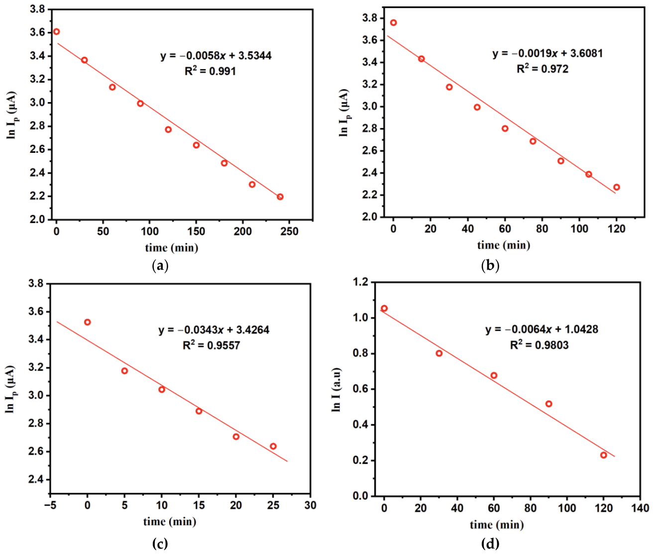
Figure 4.
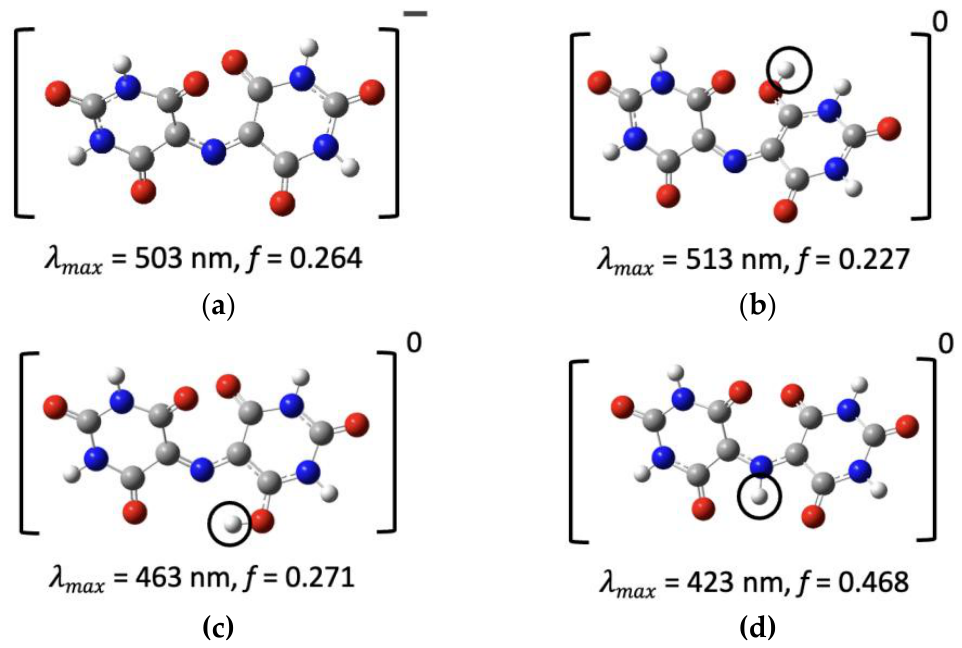
Optimized structures of (a) the purpurate anion and (b–d) the neutral species formed by protonating it at different sites. Circles mark the added proton. Each structure is labeled with its calculated absorption maximum (λmax) and oscillator strength (f). Geometries were optimized at the B3LYP-D3/6-31G (d, p) level, and TDDFT spectra were calculated at the B3LYP/6-311++G (2d, p) level with the SMD solvation model for water. Color code: C, gray; N, blue; O, red; H, white.
Figure 4.
Optimized structures of (a) the purpurate anion and (b–d) the neutral species formed by protonating it at different sites. Circles mark the added proton. Each structure is labeled with its calculated absorption maximum (λmax) and oscillator strength (f). Geometries were optimized at the B3LYP-D3/6-31G (d, p) level, and TDDFT spectra were calculated at the B3LYP/6-311++G (2d, p) level with the SMD solvation model for water. Color code: C, gray; N, blue; O, red; H, white.
UV-vis spectroscopy was used to validate the electrochemical measurements. Spectra of 5 mM murexide in acetate buffer (pH 4.9) containing 0.1 M NaClO4 were recorded every 30 min over 120 min (Figure S3d). The fresh solution showed a strong absorption band at 510 nm (A = 2.87). This band decreased steadily with time without any shift in λmax, so the solution loses its color as murexide degrades rather than forming another species that absorbs at the same wavelength. To compare the spectroscopic and electrochemical data directly, the absorbance at 510 nm was analyzed with the same pseudo-first-order model used for the peak current. A plot of ln A510 against time is linear (R2 = 0.980; Figure 4d) and gave an apparent rate constant of kobs = 0.0064 min−1 and a half-life of about 108 min. This value agrees within about 6% with the kobs obtained from the oxidation peak current over the same 120 min period (0.0068 min−1). After 120 min, 44% of the initial absorbance and 43% of the initial peak current remained. Absorbance measures the bulk concentration of the colored species, while the peak current reflects the electroactive species at the electrode, so the close agreement between the two methods confirms that the CV peak current reliably tracks the loss of murexide in solution. This validates the use of CV to determine the degradation kinetics at pH 3.0 and 2.0, where UV-vis data were not collected.
3.3. Computational Analysis
3.3.1. Origin of Photoactive Behavior of Murexide
Experimental UV-vis spectra, compared with TDDFT-calculated spectra, can help identify the dominant murexide species in acidic medium. TDDFT-calculated spectra are presented in Figure 4a–d. The experimental absorption maximum (λmax) in this study is 510 nm (Figure S3d). To find which species produces this band, we calculated the absorption spectra of the purpurate anion (Figure 4a) and three neutral species formed by protonating it at different sites (Figure 4b–d). The anion absorbs at 503 nm (f = 0.264). Protonation at the carbonyl oxygen shifts λmax to 513 nm (f = 0.227) (Figure 4b). Protonation at the other carbonyl oxygen and at the bridging nitrogen in 4 shifts the band to much shorter wavelengths: 463 nm (f = 0.271) and 423 nm (f = 0.468), respectively. These observations show that neutral purpuric acid is the dominant species.
To understand the nature of the visible absorption, we analyzed the natural transition orbitals (NTOs) of the main excitation for the purpurate anion and the O-protonated form (Figure 5a,b). In both species, the excitation is a π→π* transition centered on the C5–N–C5 bridge. The hole NTO (HOTO) lies mainly on the bridging nitrogen and the two adjacent C5 carbons, with a large contribution from the nitrogen p-orbital. The particle NTO (LUTO) spreads onto the barbiturate rings, including the C5 carbons and the neighboring carbonyl groups. The excitation therefore moves electron density from the bridge toward the rings, giving it partial intramolecular charge-transfer character. In the purpurate anion, both NTOs are symmetric across the two rings. In the O-protonated form, protonation of one carbonyl oxygen breaks this symmetry, and the particle NTO becomes unevenly distributed between the two rings. This reduces the overlap between the hole and the particle, which is consistent with the lower oscillator strength of the O-protonated form (f = 0.227 vs. 0.264) and its small red shift (513 vs. 503 nm).
Protonation of the bridging nitrogen changes this picture. In the N-protonated form (Figure 5c), the nitrogen lone pair forms the new N–H bond and the C=N bridge becomes a C–N single bond, so the nitrogen p-orbital no longer contributes to the π system. As a result, the hole NTO loses its main component on the bridge and becomes fragmented over the carbonyl and ring atoms, while the conjugation between the two barbiturate rings is interrupted. The C5–N–C5 chromophore responsible for the visible band is therefore lost, and the excitation shifts to higher energy, with a large blue shift to 443 nm [and a lower oscillator strength, f = 0.153]. Because N-protonation is also the main step of the degradation pathway, it removes the visible chromophore before the C–N bond cleaves. This is consistent with the decay of the visible absorbance in acidic solution, which follows the same kobs as the electrochemical measurements.
The possible degradation pathways of murexide in an acidic medium were investigated using DFT calculations at the B3LYP/6-31G(d,p) level with the SMD solvation model for water. Gibbs free energies were obtained at 298.15 K, and reaction free energies (ΔG) were calculated for each elementary step. Steps that involve an external proton were calculated using a free energy of −265.9 kcal/mol for the aqueous proton [30], so they depend on the solution pH. Their values at pH 2.0, 3.0, and 4.9 were obtained by adding 2.303RT·pH (1.364 kcal/mol per pH unit) to the value at pH 0. The remaining steps involve only hydration or bond cleavage and do not depend directly on pH.
The most favorable pathway is shown in Figure 6. In the first step (i), the purpurate anion (1) is protonated at the C5 carbon of one barbiturate ring, giving purpuric acid (2) (ΔG = −4.26 kcal/mol, corresponding to a calculated pKa of 3.1). Since an error of 1 kcal/mol in ΔG corresponds to about 0.7 pKa units (1/1.364), the calculated pKa lies in the range of about 2.4–3.8. This is the only pH-dependent step. Its ΔG changes from −1.53 kcal/mol at pH 2.0 to −0.17 and +2.42 kcal/mol at pH 3.0 and 4.9, so protonation is favorable at pH 2.0, close to thermoneutral at pH 3.0, and unfavorable at pH 4.9. This trend is consistent with the faster degradation observed at lower pH, where kobs increases from 0.0058 min−1 at pH 4.9 to 0.0343 min−1 at pH 2.0 (Table 3). Protonation also converts the C5 carbon from sp2 to sp3, which interrupts the C5–N–C5 conjugation responsible for the visible absorption (Figure 5). This is consistent with the loss of the purple color during degradation.
In the second step (ii), water adds across the C=N bond of 2, placing a hydroxyl group on the C5 carbon of the other ring and a hydrogen on the bridging nitrogen, which forms the carbinolamine intermediate (3) (ΔG = +1.74 kcal/mol). In the final step (iii), the C–N bond between the hydroxylated carbon and the bridging nitrogen breaks, releasing uramil (4) and alloxan (5) (ΔG = +1.12 kcal/mol). Both steps are only slightly uphill, with a combined free energy of 2.86 kcal/mol, so once purpuric acid forms, the subsequent hydration and C–N cleavage are thermodynamically accessible at room temperature. The overall reaction free energy is −1.4 kcal/mol at pH 0. Alloxan and uramil are the known hydrolysis products of murexide [21,43], which supports the proposed pathway. In the scheme, blue marks the transferred (acidic) proton and red marks the atoms that come from water.
4. Discussion
This work examined the acid-catalyzed degradation of murexide using cyclic voltammetry, UV-vis spectroscopy, and DFT/TDDFT calculations. The working hypothesis was that the instability of murexide in acidic media begins with protonation of the purpurate anion, and that the resulting species hydrolyzes at the C–N bridge. Lower pH increases the protonation of the purpurate anion and therefore the concentration of purpuric acid (2), which then undergoes degradation. The experimental and computational results support this picture and also show how a simple, inexpensive dye can be used to connect electrode kinetics, solution kinetics, and molecular-level calculations within a single system.
The kinetic measurements show that murexide degrades by pseudo-first-order kinetics at all three pH values, with kobs increasing from 0.0058 min−1 at pH 4.9 to 0.0119 and 0.0343 min−1 at pH 3.0 and 2.0. The corresponding half-lives decrease from 119 to 58 and 20 min. The kobs obtained from UV-vis absorbance at pH 4.9 (0.006 min−1) matches the electrochemical value, which shows that the decrease in peak current and the loss of the visible band track the same process. The instability of murexide in acidic solution has long been recognized from its use as a metallochromic indicator [15,16], but quantitative rate constants at lower pH are less commonly reported. The present data provide detailed kinetics of Murexide degradation.
The DFT results provide a molecular explanation for this pH dependence. Protonation of the purpurate anion at C5 to form purpuric acid is the only pH-dependent step in the most favorable pathway, with a calculated pKa of 3.1 (about 2.4–3.8 when an error of 1 kcal/mol is considered). Protonation is therefore favorable at pH 2.0, close to thermoneutral at pH 3.0, and unfavorable at pH 4.9, which follows the trend in kobs. Once purpuric acid forms, hydration of the C=N bond and C–N cleavage are only slightly uphill (2.86 kcal/mol combined) and give alloxan and uramil, the known hydrolysis products of murexide [21,43].
The TDDFT analysis connects these structural changes to the optical response. The visible band arises from a π→π* excitation centered on the C5–N–C5 bridge, with the hole located mainly on the bridging nitrogen. O-protonation breaks the symmetry of the particle NTO and produces only a small red shift (513 vs. 503 nm) and a lower oscillator strength. In contrast, protonation at C5 or at the bridging nitrogen interrupts the bridge conjugation, and N-protonation shifts the excitation to 423 nm. This explains why the purple color is lost during acid treatment and supports the use of the visible absorbance as a probe of the degradation.
The electrochemical parameters show that electron transfer of murexide at Pt is slow. The peak separation of 730–742 mV lies well outside the range of the Nicholson method, so k0 was evaluated with the Klingler–Kochi method, giving (1.4 ± 0.4) × 10−3 cm s−1. The Gileadi method gave a higher value (7.21 × 10⁻³ cm s−1), but the small shift in Ep over the scan-rate range made the critical scan rate difficult to locate, so this value is treated as an upper estimate. A similar difference between these two methods has been reported previously [35,37,38]. The slope of log Ip versus log υ (0.665) indicates mixed diffusion and adsorption control, and the increase of k0 with scan rate, together with the nearly constant ΔEp, suggests that a following chemical step contributes to the response. These observations agree with the degradation kinetics and DFT results, and they show why the choice of method and an awareness of its assumptions matter when k0 is reported for a non-ideal system.
From an educational perspective, murexide brings together several concepts that are usually taught separately: reaction order and half-life, the Randles–Ševčík relation, transfer coefficients, the comparison of k0 methods, pH-dependent free energies, and the link between frontier orbitals and color. The system shows students that different methods can give different answers, and that interpreting these differences is part of the analysis. The same workflow can be transferred to other redox-active dyes and to research problems in which acid-catalyzed degradation limits the stability of organic electrolytes or sensors.
Several directions could extend this work. UV-vis measurements at pH 2.0 and 3.0 would confirm that the spectroscopic and electrochemical rate constants agree across the full pH range. Experiments at several initial concentrations would establish the true reaction order and allow the apparent rate constants to be converted to intrinsic values. Faster scan rates, iR compensation, and digital simulation of the voltammograms with an EC mechanism would give a more reliable k0 and α. On the computational side, transition-state calculations and explicit water molecules for proton transfer would provide activation barriers rather than reaction free energies alone. Finally, product identification by NMR or mass spectrometry would directly test the predicted formation of alloxan and uramil.
5. Conclusions
Murexide (ammonium purpurate) is a purple dye that has long been used as a metallochromic indicator for Ca2+ and other metal ions [15,16,17,18]. It is also known to be unstable in acidic solution, where it loses its color and hydrolyzes to alloxan and uramil [21,43]. However, quantitative rate constants for this degradation across pH, and a molecular explanation of why protonation leads to hydrolysis, have received little attention. Murexide is inexpensive, redox-active, and strongly colored, so its degradation can be followed both electrochemically and spectroscopically, which makes it a useful model system for connecting solution kinetics, electrode kinetics, and quantum-chemical calculations. In this work, we studied the acid-catalyzed degradation of murexide at pH 4.9, 3.0, and 2.0 using cyclic voltammetry and UV-vis spectroscopy. We evaluated its heterogeneous electron transfer kinetics with the Klingler–Kochi and Gileadi methods and used DFT and TDDFT calculations to identify the protonation site that drives hydrolysis and to explain the loss of the visible absorption. The combined approach is also intended as an accessible framework for teaching how different experimental and computational methods can be used to interpret the same chemical process.
Supplementary Materials
The following supporting information can be downloaded at the website of this paper posted on Preprints.org, Table S1: Basic parameters of 5 mM murexide at pH 4.9; Table S2: Derived parameters of 5 mM murexide at pH 4.9; Figure S1: Cathodic peak current of 5 mM murexide versus (a) the square root of the scan rate and (b) the scan rate; Figure S2: Tafel plot of 5 mM murexide at pH 4.9 recorded at 0.5 V s−1; Table S3: Time-dependent peak currents of 5 mM murexide at pH 4.9, 3.0, and 2.0; Figure S3: Time-dependent degradation of 5 mM murexide at pH 4.9, 3.0, and 2.0, and UV-vis spectra at pH 4.9.
Author Contributions
S.A.R. and H.M. contributed equally. Conceptualization, Z.M., H.M. and I.A.T.; methodology and investigation, S.A.R., Z.S., A.S., H.M. and Z.M.; writing—first draft preparation, S.A.R., H.M., Z.M.; supervision, Z.M. and I.A.T.; writing—review and editing, Z.M., K.Y., I.A.T., Z.S., and H.M. All authors have read and agreed to the published version of the manuscript.
Funding
This research received no external funding.
Institutional Review Board Statement
Not applicable.
Informed Consent Statement
Not applicable.
Data Availability Statement
Not applicable.
Acknowledgments
All the computing for this project was performed at the OU Supercomputing Center for Education & Research (OSCER) at the University of Oklahoma (OU).
Conflicts of Interest
The authors declare no conflicts of interest.
References
- Waterman, K.C.; Adami, R.C. Accelerated aging: Prediction of chemical stability of pharmaceuticals. Int. J. Pharm. 2005, 293, 101–125. [Google Scholar] [CrossRef] [PubMed]
- Blessy, M.; Patel, R.D.; Prajapati, P.N.; Agrawal, Y. Development of forced degradation and stability indicating studies of drugs—A review. J. Pharm. Anal. 2014, 4, 159–165. [Google Scholar] [CrossRef] [PubMed]
- Castañeda-Ovando, A.; Pacheco-Hernández, M.d.L.; Páez-Hernández, M.E.; Rodríguez, J.A.; Galán-Vidal, C.A. Chemical studies of anthocyanins: A review. Food Chem. 2009, 113, 859–871. [Google Scholar] [CrossRef]
- Wijesekara, T.; Xu, B. A critical review on the stability of natural food pigments and stabilization techniques. Food Res. Int. 2024, 179, 114011. [Google Scholar] [CrossRef] [PubMed]
- Winsberg, J.; Hagemann, T.; Janoschka, T.; Hager, M.D.; Schubert, U.S. Redox-Flow Batteries: From Metals to Organic Redox-Active Materials. Angew. Chem. Int. Ed. 2017, 56, 686–711. [Google Scholar] [CrossRef]
- Kwabi, D.G.; Ji, Y.; Aziz, M.J. Electrolyte Lifetime in Aqueous Organic Redox Flow Batteries: A Critical Review. Chem. Rev. 2020, 120, 6467–6489. [Google Scholar] [CrossRef] [PubMed]
- Mabey, W.; Mill, T. Critical review of hydrolysis of organic compounds in water under environmental conditions. J. Phys. Chem. Ref. Data 1978, 7, 383–415. [Google Scholar] [CrossRef]
- Schwarzenbach, R.P.; Gschwend, P.M.; Imboden, D.M. Environmental organic chemistry; John Wiley & Sons, 2016. [Google Scholar]
- Bakshi, M.; Singh, S. Development of validated stability-indicating assay methods—critical review. J. Pharm. Biomed. Anal. 2002, 28, 1011–1040. [Google Scholar] [CrossRef] [PubMed]
- Gomez, M.V.; de la Hoz, A. NMR reaction monitoring in flow synthesis. Beilstein J. Org. Chem. 2017, 13, 285–300. [Google Scholar] [CrossRef] [PubMed]
- Goodson, B.M.; Ge, Q.; Wang, L. Development and Implementation of a Two-Level Inquiry- and Project-Based Modular Approach to Teaching a Second-Semester Physical Chemistry Laboratory Course. J. Chem. Educ. 2023, 100, 1885–1894. [Google Scholar] [CrossRef]
- Elgrishi, N.m.; Rountree, K.J.; McCarthy, B.D.; Rountree, E.S.; Eisenhart, T.T.; Dempsey, J.L. A Practical Beginner’s Guide to Cyclic Voltammetry. J. Chem. Educ. 2018, 95, 197–206. [Google Scholar] [CrossRef]
- Al Fulaiti, H.; Cole, A.; Balabanoff, M.; Moon, A. Toward a Model of Cognition for UV/Vis Spectroscopy. J. Chem. Educ. 2024, 101, 3062–3071. [Google Scholar] [CrossRef]
- Esselman, B.J.; Hill, N.J. Integration of Computational Chemistry into the Undergraduate Organic Chemistry Laboratory Curriculum. J. Chem. Educ. 2016, 93, 932–936. [Google Scholar] [CrossRef]
- Elsherif, K.M.; Alzalouk, Z.Y.; Zubi, A.; Al-Ddarwish, S.A.-S. Facile spectrophotometric determination of Cd (II) and Pb (II) using murexide reagent in mixed solvent system. Chem. Int. 2022, 8, 148–156. [Google Scholar]
- Khan, T.K.; Gupta-Bhaya, P. Accurate values of stability constant of Ca2+-murexide complex. Talanta 1997, 44, 2087–2094. [Google Scholar] [CrossRef]
- Elsherif, K.M.; Hadidan, Q.; Alkariwi, K. Spectrophotometric determination of Zn (II) and Cu (II) in analytical sample using murexide reagent. Prog. Chem. Biochem. Res. 2022, 5, 229–238. [Google Scholar]
- Huang, K.-H.; Tseng, C.-C.; Lee, C.-C.; Yu, C.-X.; Fu, L.-M. Rapid Finger-Pump Microfluidic Paper-Based Assay Platform for Monitoring Calcium Ions in Human Biofluids. Biosensors 2026, 16, 183. [Google Scholar] [CrossRef] [PubMed]
- Knoche, W.; Rees, N.H. The kinetics and mechanism of the decomposition of murexide in acid solution. J. Chem. Educ. 1984, 61, 724–724. [Google Scholar] [CrossRef]
- Mohran, H.S. An electrochemical investigation of the redox properties of murexide in aqueous and non-aqueous media. Am. J. Appl. Sci. 2009, 6, 964. [Google Scholar] [CrossRef]
- Ramaiah, N.; Gupta, S.; Vishnu. Studies on the kinetics of the decomposition of murexide in acid solutions. In Proceedings of the Proceedings of the Indian Academy of Sciences-Section A, 1956; pp. 286–296. [Google Scholar]
- Abidin, Z.U.; Majeed, A.; Iqbal, M.A.; Kashif, M.; Fatima, T.; Yousif, M.; Arbaz, M.; Hussain, S.A.; Sajid, M. Green and cost-effective photocatalytic degradation of murexide dye with acid catalyst. Clean Technol. Environ. Policy 2025, 27, 3333–3347. [Google Scholar] [CrossRef]
- Nicholson, R.S.; Shain, I. Theory of stationary electrode polarography. Single scan and cyclic methods applied to reversible, irreversible, and kinetic systems. Anal. Chem. 1964, 36, 706–723. [Google Scholar] [CrossRef]
- Frisch, M.J.; Trucks, G.W.; Schlegel, H.B.; Scuseria, G.E.; Robb, M.A.; Cheeseman, J.R.; Scalmani, G.; Barone, V.; Petersson, G.A.; Nakatsuji, H.; et al. Gaussian 16 Rev. B.01; Wallingford, CT, 2016. [Google Scholar]
- Stephens, P.J.; Devlin, F.; Chabalowski, C.; Frisch, M.J. Ab initio calculation of vibrational absorption and circular dichroism spectra using density functional force fields. J. Phys. Chem. 1994, 98, 11623–11627. [Google Scholar] [CrossRef]
- Grimme, S.; Antony, J.; Ehrlich, S.; Krieg, H. A consistent and accurate ab initio parametrization of density functional dispersion correction (DFT-D) for the 94 elements H-Pu. J. Chem. Phys. 2010, 132, 154104–154123. [Google Scholar] [CrossRef] [PubMed]
- Masood, Z.; Ge, Q. Electrochemical reduction of CO2 to CO and HCOO− using metal–cyclam complex catalysts: predicting selectivity and limiting potential from DFT. Dalton Trans. 2021, 50, 11446–11457. [Google Scholar] [CrossRef] [PubMed]
- Masood, Z.; Ge, Q. Mechanism and Selectivity of Electrochemical Reduction of CO2 on Metalloporphyrin Catalysts from DFT Studies. Molecules 2023, 28, 375. [Google Scholar] [CrossRef] [PubMed]
- Liu, Q.; Peng, Y.; Masood, Z.; DuBois, D.; Tressel, J.; Nichols, F.; Ashby, P.; Mercado, R.; Assafa, T.; Pan, D.; et al. Stable Cuprous Hydroxide Nanostructures by Organic Ligand Functionalization. Adv. Mater. 2023, 35, 2208665. [Google Scholar] [CrossRef] [PubMed]
- Kelly, C.P.; Cramer, C.J.; Truhlar, D.G. Aqueous solvation free energies of ions and ion− water clusters based on an accurate value for the absolute aqueous solvation free energy of the proton. J. Phys. Chem. B 2006, 110, 16066–16081. [Google Scholar] [CrossRef] [PubMed]
- Bard, A.J.; Faulkner, L.R. Fundamentals and applications: electrochemical methods. Electrochem. Methods 2001, 2, 580–632. [Google Scholar]
- Guidelli, R. Definition of the transfer coefficient in electrochemistry (IUPAC Recommendations 2014). Pure and Applied Chemistry 2000. [Google Scholar]
- Yaghoubian, H.; Karimi-Maleh, H.; Khalilzadeh, M.A.; Karimi, F. Electrocatalytic oxidation of levodopa at a ferrocene modified carbon nanotube paste electrode. Int. J. Electrochem. Sci. 2009, 4, 993–1003. [Google Scholar] [CrossRef]
- Ngamchuea, K.; Eloul, S.; Tschulik, K.; Compton, R.G. Planar diffusion to macro disc electrodes—what electrode size is required for the Cottrell and Randles-Sevcik equations to apply quantitatively? J. Solid State Electrochem. 2014, 18, 3251–3257. [Google Scholar] [CrossRef]
- Bhatti, N.K.; Subhani, M.S.; Khan, A.Y.; Qureshi, R.; Rahman, A. Heterogeneous electron transfer rate constants of viologen monocations at a platinum disk electrode. Turk. J. Chem. 2006, 30, 165–180. [Google Scholar]
- Santos, R.S.; Felipe, L.F.; Meloni, G.N. Theory in Practice: Testing the Limits of the Randles–Ševčík Equation. Acs Electrochem. 2026, 2, 478–485. [Google Scholar] [CrossRef]
- Masood, Z.; Muhammad, H.; Tahiri, I.A. Comparison of Different Electrochemical Methodologies for Electrode Reactions: A Case Study of Paracetamol. Electrochem 2024, 5, 57–69. [Google Scholar] [CrossRef]
- Muhammad, H.; Tahiri, I.A.; Muhammad, M.; Masood, Z.; Versiani, M.A.; Khaliq, O.; Latif, M.; Hanif, M. A comprehensive heterogeneous electron transfer rate constant evaluation of dissolved oxygen in DMSO at glassy carbon electrode measured by different electrochemical methods. J. Electroanal. Chem. 2016, 775, 157–162. [Google Scholar] [CrossRef]
- Nicholson, R.S. Theory and application of cyclic voltammetry for measurement of electrode reaction kinetics. Anal. Chem. 1965, 37, 1351–1355. [Google Scholar] [CrossRef]
- Lavagnini, I.; Antiochia, R.; Magno, F. An extended method for the practical evaluation of the standard rate constant from cyclic voltammetric data. Electroanal. An. Int. J. Devoted To Fundam. Pract. Asp. Electroanal. 2004, 16, 505–506. [Google Scholar] [CrossRef]
- Klingler, R.; Kochi, J. Electron-transfer kinetics from cyclic voltammetry. Quantitative description of electrochemical reversibility. J. Phys. Chem. 1981, 85, 1731–1741. [Google Scholar] [CrossRef]
- Eisner, U.; Gileadi, E. Anodic oxidation of hydrazine and its derivatives: Part I. The oxidation of hydrazine on gold electrodes in acid solutions. J. Electroanal. Chem. Interfacial Electrochem. 1970, 28, 81–92. [Google Scholar] [CrossRef]
- Knoche, W.; Rees, N.H. The kinetics and mechanism of the decomposition of murexide in acid solution. J. Chem. Educ. 1984, 61, 724. [Google Scholar] [CrossRef]
Figure 1.
(a) Cyclic voltammograms of 5 mM murexide in 0.2 M acetate buffer (pH 4.9) containing 0.1 M NaClO4 at scan rates of 0.1–0.5 V s−1. (b) Plot of log anodic peak current versus log scan rate (slope = 0.665, R2 = 0.997). W.E.: Pt; R.E.: SCE; C.E.: Pt wire.
Figure 1.
(a) Cyclic voltammograms of 5 mM murexide in 0.2 M acetate buffer (pH 4.9) containing 0.1 M NaClO4 at scan rates of 0.1–0.5 V s−1. (b) Plot of log anodic peak current versus log scan rate (slope = 0.665, R2 = 0.997). W.E.: Pt; R.E.: SCE; C.E.: Pt wire.
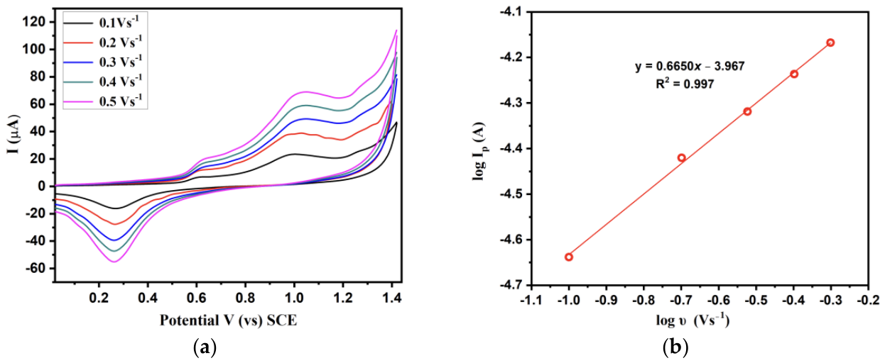
Figure 2.
Plot of the peak potential and log of scan rate of 5 mM murexide in 0.2 M acetate buffer of pH 4.9 in 0.1 M NaClO4 (W.E: Pt, R.E: SCE, C.E: Pt wire).
Figure 2.
Plot of the peak potential and log of scan rate of 5 mM murexide in 0.2 M acetate buffer of pH 4.9 in 0.1 M NaClO4 (W.E: Pt, R.E: SCE, C.E: Pt wire).
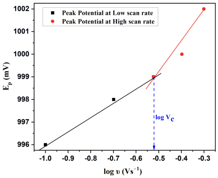
Figure 5.
Natural transition orbitals for the main visible excitation of (a) the purpurate anion, (b) the O-protonated form, and (c) the N-protonated form: particle (LUTO, top) and hole (HOTO, bottom) NTOs. Calculated at the TD-DFT B3LYP/6-311++G(2d,p) level with SMD water. Isovalue: 0.04.
Figure 5.
Natural transition orbitals for the main visible excitation of (a) the purpurate anion, (b) the O-protonated form, and (c) the N-protonated form: particle (LUTO, top) and hole (HOTO, bottom) NTOs. Calculated at the TD-DFT B3LYP/6-311++G(2d,p) level with SMD water. Isovalue: 0.04.
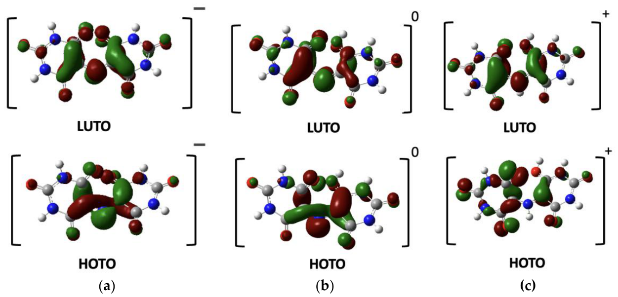
Figure 6.
Proposed pathway for the acid-catalyzed hydrolysis of murexide. Proton transfer from the hydroxyl oxygen to the bridging nitrogen (blue) is followed by addition of water (red) at C5 and cleavage of the C–N bond, giving uramil and alloxan. Blue marks the transferred proton, and red marks atoms that come from water.
Figure 6.
Proposed pathway for the acid-catalyzed hydrolysis of murexide. Proton transfer from the hydroxyl oxygen to the bridging nitrogen (blue) is followed by addition of water (red) at C5 and cleavage of the C–N bond, giving uramil and alloxan. Blue marks the transferred proton, and red marks atoms that come from water.
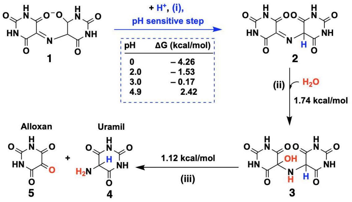

Table 1.
Diffusion coefficients (D0) of 5 mM murexide in 0.2 M acetate buffer (pH 4.9) calculated from Eq. 2 using the anodic peak currents (Ip) at different scan rates.
Table 1.
Diffusion coefficients (D0) of 5 mM murexide in 0.2 M acetate buffer (pH 4.9) calculated from Eq. 2 using the anodic peak currents (Ip) at different scan rates.
| Scan rate (V/s) | Ip(μA) | D0 (cm2/s) | |
| 0.1 | 23 | 3.87 × 10⁻⁶ | |
| 0.2 | 38 | 5.95 × 10⁻⁶ | |
| 0.3 | 48 | 7.26 × 10⁻⁶ | |
| 0.4 | 58 | 8.29 × 10⁻⁶ | |
| 0.5 | 68 | 9.53 × 10⁻⁶ | |
| Average | 6.98 × 10⁻⁶ |
Table 2.
Apparent standard heterogeneous rate constants (k0) for 5 mM murexide at pH 4.9 calculated from Eq. 7 (Klingler–Kochi method) at different scan rates. ΔEp = Epa − Epc; α = 0.32, n = 1, D0 = 5.83 × 10⁻⁵ cm2 s−1, T = 298 K.
Table 2.
Apparent standard heterogeneous rate constants (k0) for 5 mM murexide at pH 4.9 calculated from Eq. 7 (Klingler–Kochi method) at different scan rates. ΔEp = Epa − Epc; α = 0.32, n = 1, D0 = 5.83 × 10⁻⁵ cm2 s−1, T = 298 K.
| Scan rate (V s-1) | ΔEp (V) | k0 (cm s-1) | |
| 0.1 | 0.730 | 3.2 × 10⁻⁴ | |
| 0.2 | 0.731 | 4.5 × 10⁻⁴ | |
| 0.3 | 0.734 | 5.4 × 10⁻⁴ | |
| 0.4 | 0.738 | 6.2 × 10⁻⁴ | |
| 0.5 | 0.742 | 6.8 × 10⁻⁴ | |
| Average | 5.2 × 10⁻⁴ |
Table 3.
Apparent pseudo-first-order rate constants (kobs), half-lives (t1/2), and coefficients of determination (R2) for the degradation of 5 mM murexide at pH 4.9, 3.0, and 2.0. Values were obtained from linear fits of ln (Ip) versus time, with t1/2 = ln 2/kobs.
Table 3.
Apparent pseudo-first-order rate constants (kobs), half-lives (t1/2), and coefficients of determination (R2) for the degradation of 5 mM murexide at pH 4.9, 3.0, and 2.0. Values were obtained from linear fits of ln (Ip) versus time, with t1/2 = ln 2/kobs.
| pH | kobs (min–) | t1/2 (min) | R2 |
| 4.9 | 0.0058 | 119 | 0.991 |
| 3 | 0.0119 | 58 | 0.973 |
| 2 | 0.0343 | 20 | 0.956 |
Disclaimer/Publisher’s Note: The statements, opinions and data contained in all publications are solely those of the individual author(s) and contributor(s) and not of MDPI and/or the editor(s). MDPI and/or the editor(s) disclaim responsibility for any injury to people or property resulting from any ideas, methods, instructions or products referred to in the content. |
© 2026 by the authors. Licensee MDPI, Basel, Switzerland. This article is an open access article distributed under the terms and conditions of the Creative Commons Attribution (CC BY) license (http://creativecommons.org/licenses/by/4.0/).
Copyright: This open access article is published under a Creative Commons CC BY 4.0 license, which permit the free download, distribution, and reuse, provided that the author and preprint are cited in any reuse.