

Submitted:
14 November 2026
Posted:
17 November 2026
You are already at the latest version
Abstract
Phasor measurement units (PMUs) lose GPS time and enter holdover on a local oscillator, whose drift rotates every reported phasor. How long holdover can last before generator dynamic state estimation degrades remains unquantified. We study an extended Kalman filter on the IEEE 39-bus system against an ANDES simulation with stochastic loads and field-level PMU noise, under a pre-specified analysis plan. We derive a closed form for the share of PMU phase drift reaching rotor-angle estimates; it matched all 21 tested cases within 3%. This share depends on the filter’s weighting of active power against voltage angle. With noise variances calibrated to the innovations, a drifting PMU passed up to 3.0 times its phase error into the rotor angles. With compensated quartz, the error reached 0.005 rad (0.29°) after 3.5–11 min, before the PMU’s own angle error (14.7 min). Weighting power more heavily cut the pass-through 13–32-fold at the simulated locations and had the lower no-drift error (2.4 against 3.2 mrad). A clock-aware filter removed drift at some cost in ambient accuracy; with power measurements, an innovation test detected every simulated single-PMU drift without holdover flags. Holdover tolerance depends on the estimator’s weighting as much as on the oscillator.
Keywords:
dynamic state estimation
; phasor measurement unit
; GPS holdover
; clock drift
; oscillator
; extended Kalman filter
; measurement weighting
; time synchronization
1. Introduction
Phasor measurement units (PMUs) time-stamp voltage and current phasors against a common time reference, normally the Global Positioning System (GPS). This common reference is what makes phasors from distant substations comparable, and it is also a weak point. The synchrophasor standard bounds the total vector error (TVE) at 1% [1]; at 60 Hz, a timing error of 26.5 µs alone produces a phase error of 0.01 rad (0.57°) and uses up that whole budget.
Loss of the GPS signal is not rare. In phasor-data-concentrator records from the U.S. Eastern Interconnection, every deployed PMU had GPS-loss episodes, more than 60% of them lost the signal more than once a day on average, and most losses recovered within 30 min [2]. During such an outage the PMU keeps time with its local oscillator, a mode known as holdover, and its reported phase angles drift. How fast they drift depends on the oscillator. Laboratory tests of free-running quartz oscillators in frequency-disturbance recorders show the drift exceeding 1% TVE within minutes, and frequency-hold compensation extends this to about 48 min [2]. Better oscillators go further: a double-oven crystal oscillator (DOCXO) drifted about 1.8 µs in 3 h [3], and a chip-scale atomic clock about 0.89 µs in 24 h [4]. Timing error can also be imposed deliberately. On a commercial wide-area monitoring testbed, a slow GPS-spoofing attack accumulated 500 µs in 12 h without raising an alarm [5]. The receivers kept satellite lock and reported good time quality throughout, so the PMU never entered holdover. Yet the attack’s average rate, , lies within the range of compensated quartz oscillators, so its effect on the measurements resembles that of an ordinary holdover.
These figures describe the PMU itself. What they do not tell an operator is how long a PMU can remain in holdover before an application built on its data degrades. Application-level tolerance has been studied for wide-area monitoring, protection and control functions [6] and for event location, oscillation detection, islanding detection and dynamic line rating [7], but the Oak Ridge National Laboratory (ORNL) study contains no state-estimation case and no rotor-angle accuracy requirement [7]. Generator dynamic state estimation (DSE) tracks the rotor angles, speeds and internal voltages of synchronous machines from PMU data, for monitoring and control [8,9]. Common centralized formulations use an extended Kalman filter (EKF) with PMU voltage angles as direct measurements [10], which makes it a natural place for a timing error to do harm. To our knowledge, its accuracy under holdover has not been quantified.
1.1. Related Work and Research Gap
Timing errors in state estimation (SE) have been studied mainly at the network level. Yang et al. estimated bus voltages with PMUs whose clocks drift linearly between periodic re-synchronizations. They reported the estimation error against the re-synchronization interval, on a scale of seconds, and estimated the phase mismatch jointly with the state [11]. A related analysis used the posterior Cramér–Rao bound for PMU placement under random phase-angle mismatch [12]. Todescato et al. augmented a recursive Kalman filter of a distribution network’s state with each PMU’s clock offset and frequency deviation, with GPS re-synchronization every second [13,14]. Risbud et al. estimated time-varying spoofing offsets in a multi-period network model, and noted that earlier dynamic estimators with imperfect synchronization assume that GPS eventually restores it [15]. Shereen et al. showed that time-synchronization attacks can evade PMU-based state estimation [16].
In generator DSE, timing has been treated mostly as an attack to detect. Pradhan et al. applied two step offsets of 18° and 180° to one PMU of the Western Systems Coordinating Council (WSCC) 9-bus system, tracked the rotor-angle error of a linear Kalman filter (KF) and then detected the offset [17]. Siamak et al. estimated generator states from angle-free measurements, so that the estimate is immune to spoofing, and used it to detect, localize and correct constant, ramp and oscillatory phase offsets [18]. Robust unscented Kalman filters (UKFs) treat timing error as part of an unknown, non-Gaussian measurement noise [19], and decentralized DSE from instrument-transformer signals avoids PMU time stamps altogether [20].
None of these studies reports generator-DSE accuracy against holdover time or oscillator class. Our original literature screen (961 unique records, of which 35 were coded and the closest read in full; retained screening records are included in the reproducibility package, Data Availability Statement) found nothing closer than a network-level error curve against a re-synchronization interval of seconds [11]. Table 1 summarizes the closest studies. The generator case is not a simple extension of the network case, for three reasons:
- A timing error rotates every phasor of one PMU by the same angle. A generator DSE may carry this rotation into that machine’s rotor angle, spread it to other machines through the network, or absorb it into states it cannot observe directly, such as field voltage and mechanical torque.
- An outage that affects many PMUs at once turns part of the error into a common mode. Rotor angles referred to the centre of inertia (COI) do not see that common part, to first order, so only the spread between PMUs matters.
- An estimator that knows which PMUs are in holdover, as the C37.118 status flags allow [21], can carry clock states and estimate the offset. Whether it succeeds depends on what else moves the same way: load fluctuations that the estimator’s network model does not represent shift the predicted bus angles much as a clock offset does.
1.2. Research Questions and Scope
We ask four questions about a standard EKF for generator DSE on the IEEE 39-bus system:
- When one PMU enters holdover, how much of its phase drift appears in the COI-referred rotor-angle estimates? How much spills into machines other than the one at the drifting PMU’s bus, and does this depend on whether the PMUs report active and reactive power in addition to voltage phasors?
- When all PMUs enter holdover together, each with its own oscillator, how large is the rotor-angle error caused by the spread between them?
- How much of the error does a clock-aware estimator remove, given the load information a control centre actually has? How does that compare with a linear-Gaussian bound for an estimator that models the load statistics exactly?
- For oscillator classes with published performance data, how long can holdover last before the rotor-angle error crosses each of several thresholds?
PMU placement is fixed, with one PMU at each generator terminal bus. The timing model is oscillator drift during holdover, and the same angle ramp also describes a slow spoofing attack on a single PMU. Such an attack keeps the PMU’s status at good time quality [5], so a clock-aware estimator keyed to holdover flags would not switch on, and only the results for the plain estimator transfer to it. Coordinated attacks across several PMUs designed to evade detection [16] are outside the scope. Random measurement noise and PMU calibration bias are held fixed. Fault transients are excluded from the drift metrics, because the reduced-order estimator does not track them (Section 2).
1.3. Contributions
The main contributions of this paper are the following.
- A closed-form pass-through formula. We show that the share of a slow PMU timing error that a standard EKF carries into the COI rotor angles is exactly a weighted-least-squares projection onto the model’s steady states. The formula needs only the measurement model and the relative channel weights in the measurement covariance, so it can be evaluated for every PMU before deployment, without simulation; a phasor argument explains why it exceeds one. It predicted all 21 tested Monte Carlo cases within 3%. It also shows that the weighting of active power against voltage angle decides the drift response, which varied 13–32-fold between two pre-specified tunings at the simulated locations.
- Holdover limits for generator DSE. We report the rotor-angle error as a function of holdover age, for single-PMU and wide-area outages and at both tunings. Paired runs with and without drift separate the error caused by the drift from the estimator’s own error. The results are given as the holdover age at which fixed thresholds and a self-referenced limit are crossed, and are mapped to measured and specified oscillator classes.
- Two remedies and their costs. We evaluate a clock-aware EKF that uses the holdover flags, side by side with a linear-Gaussian bound that models the loads exactly, and an innovation test that needs no flag and therefore also applies to slow spoofing.
- A test design that does not favour the estimator. The estimator does not share the model that generates the data. The reference is a full ANDES simulation with sixth-order machines, exciters, governors and stochastic loads; the estimator is a reduced two-axis model whose load information is updated only at state-estimator rates. All criteria and predictions were fixed before the corresponding results were examined, and code and reproducibility materials are deposited in Zenodo (Data Availability Statement).
2. Materials and Methods
Figure 1 shows the study in four steps, each repeated for every combination of outage scenario, clock class and estimator setting.
- Simulate. A full dynamic simulation of the IEEE 39-bus system, with detailed machines, exciters, governors and randomly varying loads, produces the true trajectories that the estimator should recover (Section 2.2).
- Measure. Ten PMUs report these trajectories with field-level noise (Section 2.3). Sixty seconds into the run, the selected PMUs lose GPS and their clocks enter holdover. From then on each clock’s error grows with holdover age and rotates every phasor of that PMU by the same angle (Section 2.4).
- Estimate. An extended Kalman filter, built on a deliberately simpler machine model than the simulation, estimates the generator states from the PMU data. It also receives load values from the energy management system (EMS), which are one to two minutes old, as in a real control centre (Section 2.5).
- Compare. Each run with drift is paired with a run without drift that shares the loads, the noise and the EMS data. The difference between the two rotor-angle errors is therefore the error caused by the drift alone, and the time it takes to cross a threshold is the holdover limit (Section 2.8).
2.1. Pre-Specified Analysis Plan
The criteria, thresholds, random seeds, estimator settings and quantitative predictions used below were recorded in a version-controlled decision log before the results they govern were produced. Later changes were added as dated amendments, each recorded before the affected results were examined. At each stage the repository state was fingerprinted (SHA-256) and time-stamped by two independent RFC 3161 timestamp authorities. Simulation outputs were stored with checksums as each job finished, and each evaluation script was tested on synthetic data with known answers before the outputs it reads existed.
The study ran in two stages. A pilot study (seeds 0–5) served as a pre-specified go/no-go test for the main experiment. Five amendments were made before its results were read. They concern the load model of the reference simulation, the estimator’s tuning check, the distinction between a covariance bound and a practical estimator, the EMS load updates, and a persistent bias in those updates. The main experiment (Section 2.9) was planned after the pilot and uses new seeds; its plan, code and predictions were fixed before any of its results existed. Separate development seeds (100–105) were used only for tuning. The order in which Section 3 presents the results was chosen after the evaluation (Section 2.8); the complete pre-specified evaluation outputs are included in the Zenodo deposit (Data Availability Statement).
2.2. Test System and Reference Simulation
The test system is the IEEE 39-bus case shipped with ANDES 2.0.0 (ieee39full.xlsx), a hybrid symbolic–numeric power-system simulation framework [22]. It has ten sixth-order synchronous machines (GENROU) with IEEEX1 exciters and TGOV1N governors, all with the shipped parameters. The ten IEEEST stabilizers are removed from the case: disabling them in place leaves frozen states with zero time constants that make the algebraic solution singular. The drift metrics compare paired runs with identical stabilizer settings, so their difference isolates the injected timing error under the same damping conditions. The BusFreq and ACEc devices, which feed no other device, are removed as well, which leaves rotor-angle trajectories in a generator-trip test unchanged. The machine at bus 39 represents the external system and carries 66.1% of the total inertia on the 100 MVA base. Figure 2 shows the network, the generator buses that carry the PMUs and the buses used in the outage and disturbance scenarios.
The reference trajectories come from ANDES time-domain simulation with its implicit trapezoidal integrator, a fixed step of 1/120 s and a Newton tolerance of , sampled at the PMU reporting rate of 30 frames/s. In dynamic simulation ANDES represents each load as a constant impedance, with and . Each of the 19 loads has its and scaled by its own factor , so that active and reactive power vary independently, giving 38 random load parameters. Each follows a mean-reverting Ornstein–Uhlenbeck (OU) process,
discretized exactly at the frame interval. The OU form has been validated against distribution-level micro-PMU data, with a fitted correlation time of about 80 s [23]. Each run starts in statistical equilibrium: the initial deviations are drawn first, the power flow is solved at those loads, and the dynamic simulation starts from that operating point. The residual initial transient is below rad in the COI frame and settles within 20 s.
The primary load model uses and s. No transmission-level estimate of was found. Dai and Tate fitted the standard deviation of 5-min load changes against zone size for New York and New Zealand [24]. For an OU process , so a measured fixes only for a given . At the load sizes of this case and s, the New Zealand fit implies – and the New York fit – at the five loads inside its training range. The primary model’s lies between them, and both stay well below the variability at which the estimator fails without drift. Because the data bound the model rather than estimate it, the experiment also covers at s. Two further load models are added to or replace the OU model: a common ramp of 6.6%/h, the 95th percentile of the morning hourly load increases of the Brazilian interconnected system in 2025 [25] (a typical rather than an extreme ramp); and a random walk of 1%/min, a stress case whose variance grows without bound.
2.3. Measurements
One PMU sits at each of the ten generator terminal buses (30–39), and this placement is fixed. Two measurement sets are compared:
- set B (primary) reports the voltage angle , the voltage magnitude and the active and reactive power P and Q (40 channels), as in centralized EKF-based generator DSE with PMU angles as measurements [10];
- set A reports and only (20 channels).
Measurement noise is independent, zero-mean and Gaussian, at field level. The worst-case median signal-to-noise ratios of 13 M-class PMUs with instrument transformers are 73 dB for and 61 dB for current [26]. Propagated through the phasor model with isotropic complex noise, they give standard deviations of rad (angle), () and (P and Q), that is – per unit (pu) on the 100 MVA base across the generators. Calibrator tests of PMUs alone give angle noise of – rad, a lower bound without instrument transformers [27]. These are ambient-noise levels: instrument-transformer ratio and phase errors act as biases and are not included. The noise is generated from the simulation seed, so a drift run, its no-drift partner and both tunings (Section 2.5) see identical noise. The pilot study used earlier, assumed levels ( rad, pu and pu).
2.4. Holdover Timing Error
For elapsed holdover time , the time error of PMU i is
where is the time error in seconds, the fractional frequency offset, its aging rate in inverse seconds, and Hz. A timing error rotates all of a PMU’s phasors by the same angle:
The rotation therefore preserves and the complex power computed at that PMU, so in the simulation it is added to the PMU’s angle channel only. The phase-only TVE, as a ratio, is
so 1% TVE corresponds to rad, or 26.5 µs at 60 Hz.
The PMU is GPS-disciplined until the outage, so . Within the 30-min window of the experiments, : the measured quartz records are described as roughly linear over that window [2]. Drift is applied to the simulated measurements only, never to the estimator’s model. The clock classes are listed in Table 2, which separates measured units from manufacturer specifications and includes GPS-disciplined oscillators (GPSDOs). Two classes span the 30-min experiments:
- free-running quartz, ;
At the compensated class’s upper bound, the PMU’s own angle error reaches 0.005 rad after 14.7 min and 0.0102 rad after 30 min, just above the 1%-TVE phase. Better oscillators do not reach the thresholds within 30 min; for them, the plain EKF’s results are extended through Equation (8) (Section 2.8). Clock-aware results are not extrapolated beyond the simulated window.
Holdover starts at s, after the filter has converged, and lasts 30 min. Three outage scenarios are simulated:
- single PMU: the PMU at bus 30, 35 or 39 enters holdover at the upper bound of its class, and the other nine stay synchronized;
- wide area: all ten PMUs enter holdover together, each with drawn log-uniformly within the class range and with a random sign;
- common mode (control case): all ten PMUs drift at the class upper bound with the same sign.
The two-axis estimator model is invariant under a common rotation of all angles, so a common offset should leave the COI rotor angles unchanged; the closed-form prediction, recorded before the runs, was at most rad per radian of offset. In the wide-area scenario, then, what reaches the rotor-angle estimates is the spread between PMUs.
2.5. Estimator
2.5.1. Machine and Network Model
The estimator deliberately differs from the reference simulation. Each machine is a two-axis model with states , , and , using the GENROU parameters on the system base:
with . In this case , saturation is zero () and the damping coefficient is zero, so the only structural difference from GENROU is the missing subtransient dynamics. Field voltage and mechanical torque are random-walk states (unknown inputs). The exciter and governor dynamics therefore remain as genuine model error, and no field or turbine measurement is needed. Each machine is a Norton source behind its transient reactance, and the network is linear, with constant-admittance loads at their nominal values. The estimator has 60 states and no load states. It integrates with fourth-order Runge–Kutta (two substeps per frame) and linearizes with , using analytic Jacobians.
As a validation, the reduced model was driven with the simulated and through a 5% step at one load. Its COI rotor angles differed from the reference by rad RMS and rad at most, against a swing of rad. Through bolted faults cleared after 0.1 s, the difference reached rad. The EKF returned below 0.01 rad 2–4 s after clearing, so fault transients are excluded from all drift metrics.
2.5.2. Load Information
Real control centres update the network model from the EMS state estimator, which in large systems runs about once a minute. PJM’s estimator, for example, is triggered every minute and delivers results in 30–45 s, with a 10-s supervisory control and data acquisition (SCADA) scan of flows and voltages [34]. Classical estimators generally run one to several minutes apart [35]. The estimator therefore receives the actual per-load scale factors every 60 s, each delivered 55 s after it applied and held until the next update, so the information is 55–115 s old. The delay corresponds to a 10-s scan, 0.5-s transport [35] and a 45-s solution. Each reported value carries a white relative error , independent per load, channel and update. This level is an assumption, of the order of the metering chain behind each value: metering-class instrument transformers alone may deviate by 0.3–1.2% at rated current (accuracy classes 0.3 to 1.2 of IEEE Std C57.13 [36]) before the transducer’s own error is added; the experiment also covers 0.5% and 2%. Because metering errors are largely persistent, a sensitivity case adds a constant relative bias per load and channel for the whole run.
2.5.3. Filter and Its Two Tunings
The EKF uses the Joseph-form covariance update and wraps angle innovations to . The process noise is diagonal. Its base diffusion per state group (, , , , , ) is , in squared state units per second, scaled by 16 on , , and . The measurement covariance R is diagonal. Because R sets how much each channel counts, and therefore how a drifting angle channel is reconciled with the rest (Section 2.8), two values of R, each produced by a pre-specified rule, are run side by side with everything else shared:
- Calibrated R: , with one factor per channel kind adjusted on the development runs until the normalized innovation variance of every kind is one. The result is for angle, , P and Q. The power channels’ innovations are about 30 times the PMU noise variance, because the reduced model and 55–115-s-old load information predict P much less well than the PMUs measure it. The per-kind variances match, but the mean normalized innovation squared (NIS) on the development seeds (100–105) is 64.0 against 40 degrees of freedom, outside the pre-specified band .
- Pilot R: the earlier assumed noise variances inflated by four on angle, and Q, with P uninflated. The pilot study’s tuning rule selected this setting (mean NIS closest to 40 among 18 combinations of R inflation and process-noise scale), and at field-level noise its mean NIS on those same development seeds is 39.6, inside the band.
The ratio of angle to active-power variance, (median over generators), is with the calibrated R and with the pilot R: the pilot tuning gives active power about 800 times more relative weight. Neither tuning is consistent frame by frame, which the deliberate model mismatch prevents. The paired extra-error metric (Section 2.8) removes the error the filter makes without drift, but the gains through which drift propagates still depend on the tuning, so both are reported.
2.6. Plain and Clock-Aware Estimators
Two estimators are compared:
- the plain EKF is the filter above, with no knowledge of holdover;
- the clock-aware EKF knows which PMUs are in holdover, since C37.118 data frames carry time-quality and synchronization flags [21]. At it adds an offset and a rate for each such PMU, with , and , where is the upper bound of the PMU’s clock class. A small rate random walk with variance per 30 min is included, and enters that PMU’s angle channel.
The clock-aware EKF’s offset-and-rate model matches the injected linear drift, which favours it. The experiment therefore adds a drift it does not model: 15 min into the holdover, the clock rate steps from the class’s lower bound to its upper bound, for the PMU at bus 35 and for all ten PMUs. The step is (free-running) or (compensated), while the filter’s rate random walk allows about over 30 min. Both estimators share the model, tuning, measurements and load updates, and neither models load dynamics.
2.7. Covariance Bound
A linearized covariance analysis gives a best case, under its assumptions, for any clock-aware estimator of the same structure. The two-axis model is linearized at equilibrium and augmented with the 38 load parameters, as OU states with their true statistics, and with clock states for the PMUs in holdover. It uses the nominal process noise and the field PMU noise without inflation. The Kalman covariance recursion then runs at 30 frames/s: 60 s with synchronized clocks, as in the simulations, followed by 30 min of holdover. The bound receives the same load information as the practical estimator (updates every 60 s with 1% white error and, for the bias case, bias states with prior standard deviation ) but ignores its age. The gap between the bound and the practical estimator combines explicit load modelling, model mismatch, linearization, data age and tuning, so it bounds what load modelling could add rather than measuring it. A pre-specified trigger would have called for a load-aware estimator if, in set B and for at least half of the outage scenarios, the bound were below 0.01 rad while the practical offset error exceeded both 0.01 rad and ten times the bound.
2.8. Rotor-Angle Metrics, Pass-Through and Thresholds
For inertias on a common base, define
Rotor-angle errors are evaluated in this centre-of-inertia frame over all ten machines. Because the bus-39 equivalent carries 66% of the weight, results are repeated in a frame over the other nine machines. The change of frame is linear, so it is computed exactly from the stored signed errors of each generator. Any error common to all machines cancels in either frame.
Two quantities are reported against holdover age, each as the maximum over generators of the absolute COI rotor-angle error:
- the extra error, the drift run minus its paired no-drift run with the same loads, noise and load updates;
- the no-drift error of the paired run, the estimator’s own accuracy.
2.8.1. Pass-Through and Its Closed Form
For single-PMU outages, the pass-through ratio is reported for every generator j, where is generator j’s extra error in a given COI frame. For a slow drift the plain filter has time to settle on a steady state of its own model, namely the one that best fits the data with weights . With H the measurement Jacobian and N a basis of the null space of the model’s drift Jacobian (the equilibria near the operating point), the response of the state to a constant angle offset is
and the pass-through is the COI-referred rotor-angle rows of G in the drifting PMU’s angle column. The structure is that of a weighted-least-squares gain restricted to the model’s steady states [37,38]; what this study adds is its use as a design check before deployment. Appendix A shows that G is exactly the DC gain of the steady-state linearized filter, because the measurements depend only on the machines’ internal voltages and the random-walk inputs and make every nearby set of internal voltages a steady state. It follows that G does not depend on the process noise; only the relative channel weights in R matter. The appendix also states the conditions (a drift slow compared with the filter’s 1.5-s time constant, small offsets, an operating point near the nominal one) and gives a phasor picture of the result. With set A the fit is exact (as many steady-state unknowns as measurements), so set A’s pass-through does not depend on the tuning at all. The values from Equation (7) for each tuning and for and (angle, and Q) were recorded as predictions before the main experiment, with a match criterion of 5% on the mean of over seeds at 1 min (compensated quartz, plain EKF).
2.8.2. Thresholds
No published rotor-angle accuracy requirement for DSE was found. The ORNL assessment of synchrophasor error impacts covers other applications and gives no state-estimation limit [7]. Two kinds of threshold are therefore used.
- Fixed thresholds: 0.005 rad (0.29°); 0.0100 rad (0.57°), the phase equivalent of 1% TVE, a PMU accuracy figure rather than an application requirement; and 0.0166 rad (0.95°). Yao et al. [2] give 0.0166 rad as the angle error that causes event-location failure, citing the ORNL report [7], but the report does not contain this figure, so it serves only as a further sweep value.
- The self-referenced holdover limit, pre-specified as the meaning of “degrades”: the holdover age at which the extra error first exceeds the estimator’s own no-drift error, both taken as the root mean square (RMS) over seeds at 1, 5, 10, 20 and 30 min. It needs no external requirement and marks the age at which clock drift becomes the larger of the estimator’s two error sources.
The error curves can also be read against the bus-angle errors that the ORNL report gives for other applications: 0.0017–0.0026 rad (±0.1–0.15∘), at which event location can change its first-responding PMU, and 0.021 rad (±1.2∘), at which its triangulation fails [7]. These are bus-angle errors, not rotor-angle requirements.
To give the main threshold a physical scale: 0.005 rad (0.29°) is the phase of a 13.3-µs time error at 60 Hz, half the 1%-TVE budget. In this system it is about twice the COI rotor-angle swing caused by a 5% step at one load (2.4 mrad, Section 2.5) and of the same order as the estimator’s own error without drift (2.4–3.2 mrad, Section 3.2). A rotor-angle error of 0.005 rad is therefore as large as the small dynamic signals that DSE tracks in normal operation, while still small against the angle excursions that matter for transient stability. Section 4.3 discusses what this means for applications of DSE.
2.8.3. Reporting
Crossing ages are reported in minutes with their range over seeds. For a fixed threshold, the age is the first second at which the extra error passes it (for the RMS over seeds and for each seed). For the self-referenced limit, it is interpolated linearly in the ratio of the two RMS values between the bracketing ages, starting from zero at the outage, as the plan specified; each seed’s extra error against its own no-drift error gives the range. A threshold not crossed within 30 min is reported as censored, not as unlimited holdover. The plan also fixed bins for these ages (< 1, 1–5, 5–10, 10–20, 20–30 and > 30 min). A case whose no-drift error more than doubles over the holdover is labelled baseline-unstable and gets no self-referenced limit. The order of presentation in Section 3 (pass-through first, then fixed thresholds, then the self-referenced limit) was decided after the evaluation, because the self-referenced limit moves with the ambient error level by construction while the fixed thresholds do not.
For single-PMU cases of the plain EKF whose self-referenced limit is not reached within 30 min, the plan specified an offset mapping,
with the pooled no-drift error and the largest pass-through over generators; it holds only while the pass-through does not depend on the offset. The extra error turned out to be linear in the offset up to the thresholds studied (Section 3.2). After the runs, the same expression was therefore applied with set to a fixed threshold and taken from the closed form, to extend the fixed-threshold limits to oscillators that do not cross within 30 min. This use is labelled as an extrapolation wherever it appears.
2.8.4. Detecting the Drifting PMU
As a secondary, pre-specified analysis, the filter’s angle innovations are recorded as 1-s means. For single-PMU outages, the test statistic is the 60-s trailing mean of the drifting PMU’s angle innovation. Its null distribution comes from the paired no-drift runs of the same case, over windows ending from 1 to 30 min into the holdover and pooled over seeds; the threshold is four times the RMS of the null statistic. The detection age is the first window end at which the drift run’s statistic exceeds it. Applying the same detector to the no-drift runs gives the empirical false-alarm count.
2.9. Main Experiment
The primary load model (, s) is simulated with 12 seeds (1000–1011); every other condition uses six (1000–1005), with the same seed numbers so that conditions share their random load and noise sequences. Each run lasts 1860 s. Each simulated load realization feeds, for one measurement set and one tuning, 25 filters: the plain no-drift run and, for each outage scenario (bus 30, 35, 39, all ten) and clock class, a plain drift run, a clock-aware drift run and its clock-aware no-drift partner. The primary load model adds the common-mode control (both sets) and the clock-rate step (set B).
The primary configuration, fixed before the pilot results were read, is set B, the ten-machine COI frame, the plain EKF, white-error EMS updates and the primary load model. Clock class, outage scenario and holdover age are reported as axes. Every other factor is varied one at a time, on set B and six seeds, at both tunings unless stated:
- estimator: and on angle, and Q (calibrated tuning only); process noise and ;
- load information: EMS error 0.5% and 2%; EMS interval 300 s; persistent bias ;
- load model: OU at s, at s, the 6.6%/h ramp and the 1%/min random walk;
- disturbances, with the primary load model, 15 min into the holdover: a 5% step in the active and reactive power of the 320-MW load at bus 15, evaluated from 5 to 30 s after the step; and a bolted three-phase fault at bus 16 cleared after 0.1 s, evaluated from 5 to 30 s after clearing. Each is compared with the undisturbed run of the same seed over the same window. The estimator is not told about either event.
Set A is run with the primary load model only: its pass-through does not depend on the tuning, and its clock-aware cases are baseline-unstable (Section 4). The evaluation script was fixed before any output existed and was run once on the archived outputs.
2.10. Implementation and Reproducibility
The simulations use Python 3.12 with ANDES 2.0.0, NumPy 2.4.6 and SciPy 1.17.1. Filters that share a simulated load realization, a measurement set and a tuning are stepped together in one vectorized EKF. Over full-length runs at both tunings, its COI rotor angles and clock-offset spreads match an independent single-run implementation within rad with set B and rad with set A, the poorly conditioned case. Every random quantity (initial loads, OU increments, measurement noise, load-update errors, load bias and wide-area clock rates) has its own random stream derived from the seed, so adding a sensitivity case leaves the primary draws unchanged. The repository versions, checksums and seed lists are included in the Zenodo reproducibility package (Data Availability Statement).
3. Results
The main experiment was evaluated once, by the evaluation script fixed before it started. Unless stated otherwise, results refer to the primary configuration: set B, plain EKF, ten-machine COI frame, the primary load model and 12 seeds. “Calibrated” and “pilot” name the two tunings of R (Section 2.5), which share everything else.
3.1. Pass-Through of a Drifting PMU
Table 3 compares the measured pass-through with the closed form of Equation (7). All 21 tested predictions met the 5% criterion, with errors from to , all of them negative. The other load-model and load-information conditions were compared for information only; 52 of their 54 values matched. The two that did not are both at bus 39 at the pilot tuning with : at s and at s.
The tuning sets the pass-through. With the calibrated R, a PMU drifting at bus 30 or bus 35 moved its own machine’s COI rotor angle by 2.4 and 3.0 times its phase error, and moved other machines by 1.2–1.3 times. A drifting PMU at bus 39, the external-system equivalent, moved its own machine by 0.51 times but the machine at bus 37 by 1.34 times. With the pilot R the same diagonal values were 0.077, 0.22 and 0.040, smaller by factors of 32, 13 and 13, and the spillover to other machines fell to 0.12–0.22. At the pilot tuning a drifting PMU at bus 35 moved another machine almost as much as its own (0.22 against 0.22 in the ten-machine frame, 0.19 in the nine-machine frame). Set A has no power channels, so its pass-through was the same at both tunings, 2.9, 3.0 and 0.54, and close to the calibrated set-B values.
Figure 3 shows the mechanism. In the closed form, the pass-through depends only on the relative weights in R. When the angle, and Q variances are scaled together against P, it follows a single curve in . Where angles dominate (left), the fit follows the angle channels almost exactly and the pass-through approaches the set-A value. Where active power dominates, it falls by one to two orders of magnitude. The calibrated R lies on the left plateau, because the calibrated power variance is 30 times the PMU noise; the pilot R lies about three decades to the right. The simulations at and fall on the calibrated curve, at 2.83 and 2.16 for bus 35.
The common-mode control confirmed that only the spread between PMUs matters. When all ten PMUs drifted at the same rate and sign, the extra error stayed below of the injected offset in all 720 tested values (every seed, holdover age, frame, estimator, measurement set and clock class), against the pre-specified limit of 0.01. No common-mode case reached any threshold.
3.2. Rotor-Angle Error Against Holdover Age
Figure 4 shows the extra error against holdover age for compensated quartz. It grew in proportion to the injected offset. With the calibrated R and a single PMU, the extra error exceeded the PMU’s own angle error throughout the holdover, by 1.3–3.0 times (the largest pass-through over generators, Table 3). Seeds differed little, because the single-PMU drift is deterministic and the seeds change only the loads and the noise. With all ten PMUs in holdover, the extra error at 30 min was 0.043 rad at the calibrated tuning and 0.0072 rad at the pilot tuning; each seed drew its own set of clock rates, which widened the band. With the pilot R, the single-PMU extra errors after 30 min were 1.2, 2.3 and 1.8 mrad at buses 30, 35 and 39, below the filter’s own no-drift error.
The pilot tuning was also the more accurate one without drift. Its no-drift error, pooled over seeds and holdover ages, was 2.4 mrad, against 3.2 mrad with the calibrated R. Neither error grew over the 30 min.
The extra error was linear in the offset up to the thresholds studied, but the calibrated response became sublinear at buses 30 and 35 at the free-running quartz offsets reached after 30 min (an observation made after the runs). In the 25 primary plain-EKF cases that crossed all three fixed thresholds, the crossing ages at 0.005, 0.0100 and 0.0166 rad scaled as ––, against the threshold ratios . The extreme values come from free-running cases that cross in under a minute and are resolved to 1 s. Equation (8), evaluated with the closed-form maximum pass-through, reproduces the simulated crossings, for example 4.9 min at bus 35 and 11.0 min at bus 39 (calibrated R, compensated quartz).
3.3. Fixed Thresholds
Table 4 gives the crossing ages. With the calibrated R and compensated quartz, a single PMU took the rotor-angle extra error past 0.005 rad in 4.9–11.0 min, and all ten PMUs together in 3.5 min (2.8–4.8 min over seeds). For comparison, the PMU’s own angle error at the class’s upper rate reaches 0.005 rad at 14.7 min. The 0.0100 rad threshold, the phase equivalent of 1% TVE, followed at 9.8–21.9 min for a single PMU and at 7.1 min for all ten. With the pilot R, no single-PMU case crossed 0.005 rad within 30 min. All ten PMUs crossed it at 20.7 min, and 4 of the 12 seeds did not cross it at all. Free-running quartz crossed all three thresholds within 2 min at the calibrated tuning and 0.005 rad within 1.6–6.4 min at the pilot tuning.
In the nine-machine frame, crossings for buses 30 and 35 and for all ten PMUs came at most 15% later than in the ten-machine frame. Bus 39 is the exception. With the external-system equivalent taken out of the reference, its calibrated compensated-quartz case no longer crossed 0.005 rad within 30 min (3.6 mrad at 30 min), and its free-running cases crossed 1.7–3.5 times later. With set A, the plain EKF gave the same crossings at both tunings: 5.1, 4.8, 9.7 and 3.3 min at 0.005 rad for buses 30, 35, 39 and all ten, close to the calibrated set-B values. With set B, the clock-aware EKF’s RMS extra error never reached 0.005 rad (Section 3.6).
3.4. Self-Referenced Limit
The pre-specified meaning of “degrades” is the age at which the extra error exceeds the estimator’s own no-drift error (Table 4, last column). With the calibrated R and compensated quartz it was 4.0, 3.3 and 7.2 min for buses 30, 35 and 39 and 2.4 min for all ten, earlier than the 0.005 rad crossings because the no-drift error is below 0.005 rad. With the pilot R, no single-PMU case reached its limit within 30 min, although individual seeds did. The pre-specified offset mapping, Equation (8) with the pooled no-drift error as , places those crossings at about 60, 32 and 39 min. All ten PMUs reached it at 9.3 min (6.0–19.1). With free-running quartz the limit came within 0.4 min at the calibrated tuning and within 0.8–3.2 min at the pilot tuning.
3.5. Sensitivity to Loads, Load Information and Tuning
Figure 5 compares the two readings over the primary configuration and 15 one-factor changes, each on six seeds. The fixed-threshold crossing hardly moved. At the calibrated tuning with the PMU at bus 35, it stayed at 4.9–5.0 min everywhere except (5.2 min) and (6.8 min), which change the weighting itself. With all ten PMUs at the pilot tuning, it stayed at 23.8–24.2 min over these six seeds (20.7 min over all 12). The self-referenced limit moved with the no-drift error: from 2.5 to 13.6 min for bus 35 at the calibrated tuning, and from 8.8 min to beyond 30 min for all ten PMUs at the pilot tuning. Over the same conditions, the measured pass-through at bus 35 (calibrated) stayed within 3.002–3.010 outside the cases.
The pre-specified comparison of time bins against the primary configuration points the same way. Of 1024 comparisons, 77 changed bin, all of them for the plain EKF with set B; of these, 67 moved by one bin, 68 moved later and 9 earlier. Examined after the fact, 73 of the 77 moved in the direction of the no-drift error. In the other four, all at , the extra error fell more than the no-drift error, as the predicted pass-through implies. A persistent EMS bias of 1% raised the no-drift error to 5.4 mrad and moved the calibrated self-referenced limits to later bins (buses 30 and 35 from 1–5 to 5–10 min, bus 39 from 5–10 to 10–20 min). It left the fixed-threshold crossings unchanged.
The filter’s consistency depended on load variability. In the primary configuration the mean NIS was 66.4 at the calibrated tuning and 39.3 at the pilot tuning, against 40 channels. Across conditions it grew with load variability, from 18 at to 993 (calibrated) and 607 (pilot) at , s. The filter is therefore overconfident wherever the load variability exceeds what its process noise covers, and its absolute errors and self-referenced limits at come from a filter that is not consistent there. The pass-through still matched its prediction in those conditions, with the two exceptions at bus 39 noted above.
3.6. Clock-Aware Estimator and the Covariance Bound
With set B, the clock-aware EKF kept the drift out of the rotor angles once its clock states had converged. Its extra error was largest at the start of holdover (at most 0.15 mrad RMS over seeds 10 s in) and stayed below rad from 1 min on, at both tunings. The unmodelled step in clock rate produced a transient. With free-running quartz at the calibrated tuning, the extra error peaked 0.3–0.5 min after the step at 2.5 mrad (bus 35) and 3.9 mrad (all ten), and fell below 0.1 mrad within 1.8–3.2 min. One seed of the all-ten case passed 0.005 rad briefly. With compensated quartz the peak was 0.35–0.55 mrad about 2 min after the step; at the pilot tuning, 0.03–0.66 mrad. By 30 min the extra error was again below rad.
The clock-aware EKF paid instead in its no-drift error. With one PMU in holdover, that error, pooled over seeds and holdover ages, was at most 0.9 mrad above the plain EKF’s (calibrated, bus 39). With all ten PMUs in holdover at the calibrated tuning, it was 12.3–12.7 mrad at 1 min. From 5 min on it stayed at 4.8–6.3 mrad with compensated quartz and 8.2–9.6 mrad with free-running quartz, against 2.9–3.4 mrad for the plain EKF. At the pilot tuning the values were 4.5 mrad at 1 min, then 2.7–3.5 mrad (compensated) and 3.6–5.1 mrad (free-running), against 2.2–2.5 mrad.
The clock-offset estimates stayed well above the covariance bound but below the trigger level. At 30 min and the calibrated tuning with compensated quartz, the RMS offset error was 0.35, 0.35 and 1.37 mrad for single PMUs at buses 30, 35 and 39, and the spread error was 2.6 mrad for all ten. The bound gave 0.037, 0.042, 0.32 and 0.46 mrad. Across the primary cases the practical error was 3.4–23 times the bound, and the largest practical error was 4.6 mrad. The pre-specified trigger for a load-aware estimator required a practical error above 0.01 rad as well as ten times the bound. It fired in no condition, so no load-aware variant was built.
With set A, the clock-aware EKF is not identifiable in steady state (Section 4). Its cases were labelled baseline-unstable in all but one instance and are not interpreted.
3.7. Disturbances During Holdover
The load step and the fault, each applied 15 min into the holdover, did not change the drift’s contribution. For the plain EKF, the RMS extra error over the evaluation window was 0.998–1.002 times its undisturbed value for the load step and 1.000–1.001 times after the fault. The total error in the same window rose by factors of 0.95–1.38 and 1.00–1.52, the events’ own estimation error. For the clock-aware EKF the extra error stayed at or below rad.
3.8. Detecting the Drifting PMU
For the plain EKF with set B, the innovation test detected the drift in all 12 seeds of every single-PMU case, at both tunings. With compensated quartz the median detection age was 4.1, 3.4 and 14.0 min at buses 30, 35 and 39 (calibrated) and 7.8, 8.6 and 14.9 min (pilot). At the pilot tuning this is well before any single-PMU case reached a threshold. With free-running quartz the medians were 1.0–1.6 min at both tunings. No case had more than 1 of its 12 no-drift runs exceeding the threshold.
Detection depended on what the drift leaves in the innovations. For the clock-aware EKF with set B, the clock states absorbed the drift, and 0–1 of 12 seeds were detected. The exception was the clock-rate step at the calibrated tuning with free-running quartz, detected in 12 of 12 seeds at a median of 15.8 min, 0.8 min after the step. At the pilot tuning the step went undetected. For the plain EKF with set A, which absorbs a single PMU’s offset into the state exactly, compensated quartz was detected in 0–1 of 12 seeds and free-running quartz in all 12 (medians 1.0–7.3 min).
4. Discussion
4.1. Why the Weighting Sets the Holdover Tolerance
A clock drifts slowly compared with the filter’s dynamics. The plain filter therefore sees each PMU’s offset as nearly constant and settles on the steady state of its model that best fits all channels, weighted by (Equation (7)). To explain an angle offset at one PMU, the model must turn the rotor angles, and that changes the power at the terminal: rotating the terminal voltage by 0.005 rad (0.29°) with the other terminals unchanged shifts its active power by 14–17 MW (Appendix A). The filter must accept either this power mismatch or the angle mismatch, and R decides which. With the calibrated R, the offset is about 22 standard deviations of the angle channel, while the power change is only 5–8 standard deviations of the inflated power channel. The filter follows the angle, and the network amplifies the offset 2.4–3.0 times at buses 30 and 35: in steady state the rotor angle sits behind the q-axis synchronous reactance, two to seven times the reactance that ties these machines to the rest of the network, so the rotor must turn further than the terminal voltage it is asked to explain. With the pilot R, the same offset is 5 standard deviations of the angle channel and the power change 28–34. The filter keeps the power, the pass-through falls to 0.04–0.22, and most of the offset stays in the angle innovations, where the test of Section 3.8 found it.
The calibrated R falls on the first side for a mundane reason. Calibrating each channel kind to its innovation variance gives the power channels 30 times the PMU noise variance, because the reduced model and 55–115-s-old load information predict active power much less well than the PMU measures it. That is a correct account of the prediction error. It also tells the filter to trust angles over power, which is the weighting most exposed to timing error. The pilot R weighted active power about 800 times more relative to angle. At the three simulated locations it reduced the pass-through 13–32-fold. Across all ten PMU locations, the closed form gives reductions of 3.3–21 times in the largest pass-through over generators, and 8.1 times between the two tunings’ worst locations (4.39 at bus 37 against 0.54 at bus 38). The pilot R also had the lower no-drift error (2.4 against 3.2 mrad) and the mean NIS closer to the channel count (39 against 66). In this system, then, weighting power over angle cost nothing, and the per-kind calibration was the costliest choice for holdover. Whether that holds elsewhere depends on how the pass-through and the no-drift error move with the weighting in another system. Because Equation (7) needs only the measurement Jacobian, the null space of the drift Jacobian and R, a designer can evaluate it for every PMU before deployment, without simulation.
With angle and voltage-magnitude channels only (set A), the weighting no longer matters. The fit is exact, and the plain EKF’s pass-through equals the shift that reproduces the offset. That shift is 2.9 times the offset at bus 30 (observed 2.86–2.87) and 3.1 times at bus 35 (observed 3.04–3.05); at bus 39 the COI frame reduces it to 0.55 (observed 0.54). The same direction makes the clock-aware EKF non-identifiable in steady state. A holdover offset at one PMU produces the same measurements as a redispatch that raises that machine’s mechanical torque and excitation, and the filter diverges along that direction even without drift. The divergence needs PMU measurement noise. With noise-free measurements the estimate does not move; with noise, its sign and rate repeat across independent noise draws. These cases were labelled baseline-unstable and are not interpreted. With power measurements (set B), no such direction exists for a single PMU.
4.2. Clock Requirements and Practical Holdover
The natural comparison is with the PMU’s own error. At the compensated quartz class’s upper rate, the PMU’s angle error reaches 0.005 rad after 14.7 min and the phase equivalent of 1% TVE after 29.5 min. With the calibrated R the rotor-angle error got there first: 0.005 rad after 4.9–11.0 min for one PMU and 3.5 min for all ten. Here the estimator, not the PMU, set the holdover limit. With the pilot R, the three simulated single-PMU locations stayed below 0.005 rad for 30 min, so the PMU’s own accuracy would bind first. All ten PMUs together crossed 0.005 rad after 20.7 min, and 4 of 12 seeds did not cross it. Free-running quartz exhausts either budget within minutes at either weighting.
Because the extra error is linear in the offset up to the thresholds studied, Equation (8) extends the single-PMU limits to better oscillators (Table 5). The extension was made after the runs, at each tuning’s worst PMU location. With the calibrated R, staying below 0.005 rad for 30 min at every location requires an oscillator well beyond compensated quartz (3.4 min at the worst location); the worst measured rubidium unit’s rate gives 50 min. With the pilot R, compensated quartz comes close (27 min at the worst location). The simulated wide-area crossings came at 0.76–1.06 times the worst single-location value (3.5 against 3.4 min calibrated, 20.7 against 27 min pilot), so a wide-area outage can shorten these times by about a quarter. Most recorded GPS losses recovered within 30 min [2]. Times of hours or days in Table 5 rest on a linear drift beyond most clocks’ measured records and on an operating point that does not change. They rank the classes and are not holdover guarantees. Figure 6 places these times on a common scale, next to the time the PMU’s own angle error needs to reach the same 0.005 rad. Because the estimator’s limit is the PMU’s divided by the worst-case pass-through, with the calibrated R the rotor angles reach it 4.4 times sooner than the PMU’s own angle, and with the pilot R they take 1.9 times as long, for every clock class.
4.3. What the Error Means for Applications of DSE
Whether a rotor-angle error of this size matters depends on what the estimates feed. The applications listed for DSE include oscillation monitoring, wide-area and excitation control, protection, and transient-stability monitoring [8], and they use the rotor angle at very different scales.
Model validation and parameter calibration compare estimated and simulated responses after small disturbances, so the relevant scale is the response itself. In this system a 5% step at one load moved the COI rotor angles by 2.4 mrad (0.14°). With compensated quartz and the calibrated R, the drift-induced error reached 5 mrad (0.29°), twice that response, after 3.5–11 min (Table 4), and an analyst would read it as a model error. This is the most exposed use, and here the 0.005 rad threshold is the appropriate one.
Oscillation monitoring and wide-area damping control act on the oscillatory part of the estimated angles and speeds. The drift error is a slow ramp, and the disturbance runs showed that it adds to the estimate without changing the estimated response to a load step or a fault (extra error 0.998–1.002 times its undisturbed value, Section 3.7). Such a function would see a slowly moving offset rather than a distorted oscillation. Whether that offset matters depends on how the function filters slow trends, which was not modelled here.
Transient-stability monitoring and out-of-step protection work with angle differences of tens of degrees, against which the compensated-quartz errors are small: at most 0.043 rad (2.5°) after 30 min, with all ten PMUs at the calibrated R. The error grows for as long as the holdover lasts, however, and with free-running quartz it reached the scale of stability margins within the simulated 30 min: 0.28–0.45 rad (16–26°) for a single PMU and 0.90 rad (51°, RMS over seeds) for all ten PMUs at the calibrated R, against 0.02–0.05 rad (1.3–2.6°) and 0.093 rad (5.4°) at the pilot R. At these large offsets, the calibrated response at buses 30 and 35 is sublinear, so the small-offset pass-through overpredicts their 30-min error (Section 3.2). For these uses, then, the oscillator class and the weighting decide whether holdover is a nuisance or a hazard; the innovation test of Section 3.8, which flagged free-running drift after a median of 1.0–1.6 min, is the obvious safeguard.
The self-referenced limit answers a different question: when clock drift becomes the larger of the estimator’s two error sources. It came earlier than the 0.005 rad crossing wherever the no-drift error was below 0.005 rad. It also moved with that error across the sensitivity cases (2.5–13.6 min at bus 35, calibrated), while the 0.005 rad crossing there stayed within 0.1 min outside the cases. Its pre-specified bins changed in 77 of 1024 comparisons, and 73 of those moved with the no-drift error. The fixed thresholds are therefore the reading that transfers between conditions. The self-referenced limit describes a particular estimator under particular loads.
4.4. What an Operator Can Do
Three remedies emerge, each with a cost. The first is the weighting itself. Equation (7) shows, for each PMU, how much a slow timing error will reach the rotor angles under a candidate R. Here the power-weighted choice was also the more accurate one without drift.
The second is a clock-aware estimator keyed to the C37.118 holdover flags. In set B it kept the drift out of the rotor angles from the first minute on, even through an unmodelled change of clock rate, although that change cost a transient of up to 3.9 mrad lasting about 3 min. Its cost is ambient accuracy when many PMUs are in holdover at once: with all ten flagged, its no-drift error rose to 12.3–12.7 mrad at entry and stayed at 1.5–3 times the plain EKF’s at the calibrated tuning. Its offset estimates were 3.4–23 times the covariance bound. The bound models the load statistics exactly, so part of this gap is what load modelling could recover. The gap also includes the reduced-model mismatch, linearization, data age and tuning. Since the practical errors stayed below 5 mrad, the pre-specified trigger for building a load-aware estimator did not fire.
The third is monitoring. The innovation test needs no flag. In set B it detected the drift at every simulated location, tuning and seed, after a median of 3.4–14.9 min with compensated quartz. It is therefore the remedy that also applies to a slow spoofing attack, which keeps the time-quality flag good [5]. The reported attack rate, , lies inside the simulated compensated-quartz range. The test detected least where the drift was absorbed into the state: in set A with compensated quartz, 0–1 of 12 seeds. Its threshold here came from paired no-drift runs; in operation it would have to come from the estimator’s own history. Power channels matter for all three remedies. Without them, the pass-through is fixed at the set-A level, the clock-aware EKF is not identifiable, and slow drift does not show in the innovations.
4.5. Limitations and Generalization
The study uses one test system, one PMU placement and one estimator family: an EKF with a two-axis machine model. A UKF, a robust filter and a second test system were not run. Its two tunings come from pre-specified rules. The continuum between them comes from the closed form, which was confirmed at three PMU locations, two tunings and two scalings of R but not across the whole curve or at the other seven locations. The worst-case pass-through used in Table 5 comes from those other locations.
The filter is not consistent everywhere. Its mean NIS grew with load variability, to 993 (calibrated) and 607 (pilot) at , s, where it is overconfident. Absolute errors and self-referenced limits at come from such a filter. The two pass-through predictions that missed, both at bus 39 at the pilot tuning with ( and ), fall where the closed form is most sensitive to the operating point. A post hoc check (Appendix A) accounts for the size of these misses but not for their consistent sign. The load statistics are bounded by distribution-level and system-level data rather than measured at transmission level, and the EMS error level is assumed. The reference simulation’s machines, controls and loads differ from the estimator’s on purpose. Fault transients are excluded from the metrics because the reduced model does not track them.
The clock model is linear: oscillator aging and temperature are not included, and single-PMU outages run at each class’s upper rate. The clock-aware EKF’s model matches the injected drift. A step in the clock rate tested it beyond that, but not against aging or temperature cycles. Measurement noise is ambient only; instrument-transformer ratio and phase errors, which act as biases, are excluded. The innovation test’s threshold was set from paired runs, and its false-alarm rate in operation is unknown. The extension of the fixed-threshold limits through Equation (8) and the all-location pass-through were derived after the runs.
The comparison with earlier work is limited by its scope. Pradhan et al. [17] found that a step offset at one PMU biased the rotor-angle estimate of a linear Kalman filter. Equation (7) gives the size of that bias for a slow offset and shows that it depends on the weighting. Network-level studies report estimation error against re-synchronization intervals of seconds [11]. Holdover lasts minutes to hours, and the present results cover that range for generator DSE. For a slow spoofing attack on one PMU, which keeps the PMU’s status good, the plain-EKF results and the innovation test transfer; the clock-aware EKF does not.
5. Conclusions
How long a PMU can stay in GPS holdover before generator DSE degrades depends on how the estimator weights active power against voltage angle. For an EKF on the IEEE 39-bus system with field-level PMU noise, the four research questions have the following answers.
- A single drifting PMU passes a fixed multiple of its phase error into the COI rotor angles. A closed form that depends only on the relative channel weights predicted the multiple within 3% in all 21 tested cases. When the filter trusted angles over power, it was 2.4–3.0 for the drifting PMU’s own machine at buses 30 and 35 (0.51 at bus 39, the external-system equivalent) and up to 1.3 for other machines. When power carried more weight it was 0.04–0.22. Without power channels it was close to the angle-trusting values (2.9, 3.0 and 0.54), whatever the weighting.
- When all PMUs drift together, only their spread reaches the rotor angles; a common drift cancelled to within of the offset. After 30 min with compensated quartz, the spread produced 0.043 rad of rotor-angle error at the angle-trusting weighting and 0.0072 rad at the power-trusting one.
- An estimator that carries clock states for the PMUs flagged in holdover kept the drift out of the rotor angles, apart from a transient of up to 4 mrad after an unmodelled change of clock rate. Its price is a larger ambient error when many PMUs are in holdover at once. Its offset estimates were 3.4–23 times a covariance bound that models the loads exactly, but below 5 mrad, so the pre-specified case for a load-aware estimator did not arise.
- With compensated quartz, the rotor-angle error reached 0.005 rad (0.29°) after 3.5–11 min at the angle-trusting weighting, earlier than the PMU’s own angle error (14.7 min). At the power-trusting weighting no simulated single-PMU outage reached it within 30 min, and all ten PMUs together reached it after 21 min. Free-running quartz reached it within minutes at either weighting.
In practice, the pass-through formula can be evaluated for every PMU from the measurement model and R before deployment. Weighting power over angle cost no accuracy here and reduced the drift response by 13–32 times at the simulated locations. A test on the drifting PMU’s angle innovations detected every simulated single-PMU drift with power channels, needs no holdover flag, and therefore also applies to slow spoofing. These conclusions rest on one test system, one estimator family and ambient measurement noise. At the highest load variability tested, the filter was overconfident.
Author Contributions
Conceptualization, L.G.P.M. and R.C.P.; methodology, L.G.P.M. and R.C.P.; software, L.G.P.M.; validation, L.G.P.M.; formal analysis, L.G.P.M.; investigation, L.G.P.M.; data curation, L.G.P.M.; writing—original draft preparation, L.G.P.M.; writing—review and editing, L.G.P.M. and R.C.P.; visualization, L.G.P.M.; supervision, R.C.P.; project administration, R.C.P. All authors have read and agreed to the published version of the manuscript.
Funding
This study was financed in part by the Coordenação de Aperfeiçoamento de Pessoal de Nível Superior – Brasil (CAPES) – Finance Code 001.
Institutional Review Board Statement
Not applicable.
Informed Consent Statement
Not applicable.
Data Availability Statement
The code, simulation outputs and reproducibility materials supporting the reported results are openly available in Zenodo at https://doi.org/10.5281/zenodo.24118296.
Conflicts of Interest
The authors declare no conflicts of interest. The funders had no role in the design of the study; in the collection, analyses, or interpretation of data; in the writing of the manuscript; or in the decision to publish the results.
Abbreviations
The following abbreviations are used in this manuscript:
| COI | Centre of inertia |
| DOCXO | Double-oven crystal oscillator |
| DSE | Dynamic state estimation |
| EKF | Extended Kalman filter |
| EMS | Energy management system |
| EPFL | École Polytechnique Fédérale de Lausanne |
| GPS | Global Positioning System |
| GPSDO | GPS-disciplined oscillator |
| KF | Kalman filter |
| NIS | Normalized innovation squared |
| ORNL | Oak Ridge National Laboratory |
| OU | Ornstein–Uhlenbeck |
| PMU | Phasor measurement unit |
| pu | Per unit |
| RMS | Root mean square |
| SCADA | Supervisory control and data acquisition |
| SE | State estimation |
| TVE | Total vector error |
| UKF | Unscented Kalman filter |
| WLS | Weighted least squares |
| WSCC | Western Systems Coordinating Council |
Appendix A. Derivation of the Pass-Through Formula
Equation (7) has a familiar structure. It is the gain of a weighted-least-squares (WLS) estimator, the same matrix that gives the sensitivity of a static state estimate to measurement errors [37], restricted to the steady states of the estimator’s dynamic model. The steady-state response of a recursive filter to a constant measurement bias has likewise been studied since the early bias-filtering literature [38]. What is shown here is that, for generator DSE and under the conditions below, it is the exact response of the steady-state filter to a slow PMU timing error. The numerical checks are post hoc.
Appendix A.1. Setting
Linearize the estimator at an equilibrium of its two-axis model, with drift Jacobian A, transition matrix and measurement Jacobian H. A timing error at PMU i adds to that PMU’s angle channel only (Equation (3)), that is, a measurement offset , with the unit vector of that channel. Let K be the steady-state Kalman gain, P the corresponding prior covariance, , and the closed-loop matrix. Because the filter is linear in its inputs, the difference between a drift run and its paired no-drift run, the extra error, obeys to first order
For a constant offset b and a stable filter (spectral radius of below one), converges to , with .
Appendix A.2. Two Structural Properties of the Generator Model
The equilibrium set. The field voltage and the mechanical torque are random-walk states, so their rows of A are zero. A steady state of Equation (5) must satisfy only the 40 conditions and on the 60 states. Near the steady states therefore form a set of dimension 20, whose tangent space is the null space of A, spanned by the columns of N (dimension 20, checked numerically). Physically, any small change of the machines’ internal voltages can be held in equilibrium by a matching change of and ; it is the treatment of these two inputs as unknown states that creates the null space. Since , also .
Measurements depend on the internal voltages only. Each machine is a Norton source behind its transient reactance and the network is linear, so the terminal voltages and currents, and hence every channel (, , P, Q), are functions of the ten complex internal voltages , that is, of 20 real coordinates. The Jacobian therefore factors as , where T maps state deviations to these 20 coordinates and maps the coordinates to the measurements. On the equilibrium set the map is one-to-one: is an invertible matrix (numerically, in both measurement sets).
Appendix A.3. The DC Gain Equals the Weighted-Least-Squares Projection
Look for the fixed point of Equation (A1) on the equilibrium set, . Because , the fixed-point condition reduces to
where r is the steady innovation. With , P positive definite and T of full row rank, holds exactly when . The matrix inversion lemma, with and , gives
and the factor in front of is invertible. Hence is equivalent to and, because is invertible, to
These are the normal equations of , whose solution is with G from Equation (7). The fixed point of a stable filter is unique, so : the filter settles on the steady state of its model that best fits the offset data in the metric .
Why the process noise drops out. The covariance P, and with it the process noise Q and the initial covariance, enters only through M, which cancels from the condition. Any positive-definite P gives the same fixed point. The process noise sets how fast the filter reaches it, not where. Scaling R as a whole also leaves G unchanged; only the relative channel weights matter. Numerically, the DC gain from the discrete algebraic Riccati equation matches G to within the accuracy of the Riccati solution ( or better in every tuning checked).
Appendix A.4. Timescale Separation
A holdover drift is a ramp, not a constant. The derivation applies to it when the drift changes slowly compared with the filter’s closed-loop dynamics, so that the filter is close to its fixed point at each instant. The slowest mode of has magnitude 0.979 per frame at both tunings, a time constant of 1.5 s, far shorter than holdover ages of minutes. Driven by a ramp that starts at the outage, Equation (A1) lags by 0.15–0.93% at 1 min for the three simulated PMUs at both tunings, which explains why all 21 tested prediction errors were negative (Section 3.1) and most of their size.
Appendix A.5. When the Formula Fails
The derivation identifies four conditions; the formula should not be trusted where one of them fails.
- Fast timing errors. Offsets that change within a few filter time constants, such as the step offsets of spoofing studies, excite the transient response of , not its fixed point.
- Large offsets. The derivation is linear. The extra error was linear in the offset up to the thresholds studied, but the calibrated response became sublinear at buses 30 and 35 at the free-running quartz offsets reached after 30 min (Section 3.2).
- Operating point.G is evaluated at the nominal equilibrium. A 5% spread of the load operating points moves the pilot-tuning pass-through at bus 39 by up to about , which covers the size of the two missed predictions there but not their sign.
- Structure. The formula needs of full column rank and an estimator that does not model the offset, so it does not apply to the clock-aware estimator. With set A, is square and invertible: any angle offset can be reproduced exactly by a steady state, so adding an offset state makes the augmented problem rank-deficient. This is the non-identifiability of the set-A clock-aware estimator (Section 4.1).
Appendix A.6. Why the Pass-Through Can Exceed One
With set A the fit is exact, so the filter must reproduce a rotation of terminal voltage while and every other terminal voltage stay as measured. In steady state the rotor angle is the angle of the voltage behind the synchronous q-axis reactance, as in the classical phasor diagram. With the other terminals held, the current changes by , where is the driving-point admittance of the network reduced to the generator terminals, with the loads as admittances. Neglecting losses, , and . The rotor angle therefore moves by
and referring it to the COI removes roughly the fraction . In the two-machine picture of Figure A1, the terminal voltage divides the path between and the rest of the system, so moving it by with the far end fixed swings like a lever. Table A1 gives the values: the approximation is within 13% of the closed form, and the same construction without approximations reproduces the set-A pass-through and spillover of Table 3 to all digits shown. Buses 30 and 35 have a q-axis reactance two to seven times ; the external-system equivalent at bus 39 has a small and two-thirds of the COI weight.
Figure A1.
Why the pass-through can exceed one (schematic, lossless, , angles exaggerated). (a) Machine i in steady state is the voltage behind its q-axis synchronous reactance; its phasor measurement unit (PMU) measures the terminal voltage ; the rest of the system, whose terminal voltages are held by their own PMUs, is represented by behind . (b) lies on the straight line from to , dividing it in the ratio . To explain a drifted terminal angle () with fixed, the model must swing about like a lever, times as far, so the rotor angle moves by more than the terminal angle ().
Figure A1.
Why the pass-through can exceed one (schematic, lossless, , angles exaggerated). (a) Machine i in steady state is the voltage behind its q-axis synchronous reactance; its phasor measurement unit (PMU) measures the terminal voltage ; the rest of the system, whose terminal voltages are held by their own PMUs, is represented by behind . (b) lies on the straight line from to , dividing it in the ratio . To explain a drifted terminal angle () with fixed, the model must swing about like a lever, times as far, so the rotor angle moves by more than the terminal angle ().


Table A1.
Phasor picture of the set-A pass-through (Equation (A5)), nominal operating point, per unit (pu) on the 100 MVA base. Approximation: Equation (A5) times . Closed form: Equation (7), set A.
| Bus | (pu) | (pu) | Approx. | Closed form | ||
|---|---|---|---|---|---|---|
| 30 | 0.066 | 0.030 | 14.3∘ | 0.92 | 2.70 | 2.90 |
| 35 | 0.222 | 0.031 | 42.3∘ | 0.50 | 2.87 | 3.06 |
| 39 | 0.016 | 0.038 | 4.9∘ | 1.00 | 0.48 | 0.55 |
With set B, the same rotation changes the active power at the terminal by 28–34 pu per radian; Section 4.1 shows how R then decides between the angle and the power residual.
References
- IEC/IEEE. Standard IEC/IEEE 60255-118-1:2018; Measuring Relays and Protection Equipment – Part 118-1: Synchrophasor for Power Systems – Measurements. IEC and IEEE, 2018. [CrossRef]
- Yao, W.; Liu, Y.; Zhou, D.; Pan, Z.; Till, M.J.; Zhao, J.; Zhu, L.; Zhan, L.; Tang, Q.; Liu, Y. Impact of GPS Signal Loss and Its Mitigation in Power System Synchronized Measurement Devices. IEEE Trans. Smart Grid 2018, 9, 1141–1149. [Google Scholar] [CrossRef]
- Yao, W.; Zhan, L.; Yin, H.; Liu, Y. PMU Holdover Performance Enhancement Using Double-Oven Controlled Oscillator. IEEE Trans. Power Deliv. 2019, 34, 2260–2262. [Google Scholar] [CrossRef]
- Zhan, L.; Liu, Y.; Yao, W.; Zhao, J.; Liu, Y. Utilization of Chip-Scale Atomic Clock for Synchrophasor Measurements. IEEE Trans. Power Deliv. 2016, 31, 2299–2300. [Google Scholar] [CrossRef]
- Kim, C.; Noh, J.; Ghahremani, E.; Kim, Y. Revisiting GPS Spoofing in Phasor Measurement: Real-World Exploitation and Practical Detection in Power Grids. ACM Trans. Priv. Secur. 2025, 28, 1–27. [Google Scholar] [CrossRef]
- Almas, M.S.; Vanfretti, L.; Singh, R.S.; Jonsdottir, G.M. Vulnerability of Synchrophasor-Based WAMPAC Applications’ to Time Synchronization Spoofing. IEEE Trans. Smart Grid 2018, 9, 4601–4612. [Google Scholar] [CrossRef]
- Zhao, J.; Tan, J.; Wu, L.; Zhan, L.; Liu, Y.; Gracia, J.R.; Ewing, P.D. 2015. Impact of Measurement Error on Synchrophasor Applications. Technical Report ORNL/TM-2015/314. Oak Ridge National Laboratory, Oak Ridge, TN, USA. [Google Scholar] [CrossRef]
- Zhao, J.; Gómez-Expósito, A.; Netto, M.; Mili, L.; Abur, A.; Terzija, V.; Kamwa, I.; Pal, B.; Singh, A.K.; Qi, J.; et al. Power System Dynamic State Estimation: Motivations, Definitions, Methodologies, and Future Work. IEEE Trans. Power Syst. 2019, 34, 3188–3198. [Google Scholar] [CrossRef]
- Zhou, N.; Meng, D.; Huang, Z.; Welch, G. Dynamic State Estimation of a Synchronous Machine Using PMU Data: A Comparative Study. IEEE Trans. Smart Grid 2015, 6, 450–460. [Google Scholar] [CrossRef]
- Netto, M.; Zhao, J.; Mili, L. A Robust Extended Kalman Filter for Power System Dynamic State Estimation Using PMU Measurements. In Proceedings of the 2016 IEEE Power and Energy Society General Meeting (PESGM), Boston, MA, USA, 17–21 July 2016; pp. 1–5. [Google Scholar] [CrossRef]
- Yang, P.; Tan, Z.; Wiesel, A.; Nehorai, A. Power System State Estimation Using PMUs With Imperfect Synchronization. IEEE Trans. Power Syst. 2013, 28, 4162–4172. [Google Scholar] [CrossRef]
- Yang, P.; Tan, Z.; Wiesel, A.; Nehorai, A. Placement of PMUs Considering Measurement Phase-Angle Mismatch. IEEE Trans. Power Deliv. 2015, 30, 914–922. [Google Scholar] [CrossRef]
- Todescato, M.; Carli, R.; Schenato, L.; Barchi, G. PMUs Clock De-Synchronization Compensation for Smart Grid State Estimation. In Proceedings of the 2017 IEEE 56th Annual Conference on Decision and Control (CDC), Melbourne, Australia, 12–15 December 2017; pp. 793–798. [Google Scholar] [CrossRef]
- Todescato, M.; Carli, R.; Schenato, L.; Barchi, G. Smart Grid State Estimation with PMUs Time Synchronization Errors. Energies 2020, 13, 5148. [Google Scholar] [CrossRef]
- Risbud, P.; Gatsis, N.; Taha, A. Multi-Period Power System State Estimation with PMUs Under GPS Spoofing Attacks. J. Mod. Power Syst. Clean Energy 2020, 8, 597–606. [Google Scholar] [CrossRef]
- Shereen, E.; Delcourt, M.; Barreto, S.; Dán, G.; Le Boudec, J.Y.; Paolone, M. Feasibility of Time-Synchronization Attacks Against PMU-Based State Estimation. IEEE Trans. Instrum. Meas. 2020, 69, 3412–3427. [Google Scholar] [CrossRef]
- Pradhan, P.; Nagananda, K.; Venkitasubramaniam, P.; Kishore, S.; Blum, R.S. GPS Spoofing Attack Characterization and Detection in Smart Grids. In Proceedings of the 2016 IEEE Conference on Communications and Network Security (CNS), Philadelphia, PA, USA, 17–19 October 2016; pp. 391–395. [Google Scholar] [CrossRef]
- Siamak, S.; Dehghani, M.; Mohammadi, M. Dynamic GPS Spoofing Attack Detection, Localization, and Measurement Correction Exploiting PMU and SCADA. IEEE Syst. J. 2021, 15, 2531–2540. [Google Scholar] [CrossRef]
- Zhao, J.; Mili, L. Robust Unscented Kalman Filter for Power System Dynamic State Estimation With Unknown Noise Statistics. IEEE Trans. Smart Grid 2019, 10, 1215–1224. [Google Scholar] [CrossRef]
- Singh, A.K.; Pal, B.C. Decentralized Robust Dynamic State Estimation in Power Systems Using Instrument Transformers. IEEE Trans. Signal Process. 2018, 66, 1541–1550. [Google Scholar] [CrossRef]
- IEEE. Standard C37.118.2-2011; IEEE Standard for Synchrophasor Data Transfer for Power Systems. IEEE, 2011. [CrossRef]
- Cui, H.; Li, F.; Tomsovic, K. Hybrid Symbolic-Numeric Framework for Power System Modeling and Analysis. IEEE Trans. Power Syst. 2021, 36, 1373–1384. [Google Scholar] [CrossRef]
- Roberts, C.; Stewart, E.M.; Milano, F. Validation of the Ornstein–Uhlenbeck Process for Load Modeling Based on μPMU Measurements. In Proceedings of the 2016 Power Systems Computation Conference (PSCC), Genoa, Italy, 20–24 June 2016; pp. 1–7. [Google Scholar] [CrossRef]
- Dai, Z.; Tate, J.E. A Data-Driven Load Fluctuation Model for Multi-Region Power Systems. IEEE Trans. Power Syst. 2019, 34, 2152–2159. [Google Scholar] [CrossRef]
- Operador Nacional do Sistema Elétrico (ONS). Curva de Carga Horária, 2025 (CURVA_CARGA_2025.csv). Available online: https://dados.ons.org.br/dataset/curva-carga (accessed on 5 March 2026).
- Constante Segura, J.R.; Colomé, D.G.; Echeverría, D.E. Noise Amplitude in Ambient PMU Data and its Impact on Load Models Identification. IEEE Lat. Am. Trans. 2024, 22, 678–685. [Google Scholar] [CrossRef]
- Salls, D.; Ramírez Torres, J.; Varghese, A.C.; Patterson, J.; Pal, A. Statistical Characterization of Random Errors Present in Synchrophasor Measurements. In Proceedings of the 2021 IEEE Power & Energy Society General Meeting (PESGM), Washington, DC, USA (virtual), 26–29 July 2021; pp. 1–5. [Google Scholar] [CrossRef]
- Taitien Electronics. NI-10M-3600 Series Double-Oven Controlled Crystal Oscillator 2026. Data sheet, Rev. 3. Available online: https://www.taitien.com/wp-content/uploads/2026/07/NI-10M-3600.pdf (accessed on 10 September 2026).
- Anastasiev, S.V.; Volkov, A.A.; Vorokhovsky, Y.L. A New High Stability DOCXO. Statistics of the Results of Frequency Stability Measurements. In Proceedings of the 2002 IEEE International Frequency Control Symposium and PDA Exhibition, New Orleans, LA, USA, 29–31 May 2002; pp. 633–638. [Google Scholar] [CrossRef]
- Microchip Technology. 45s CSAC Options 001 and 003: Chip-Scale Atomic Clock. In 2023. Data sheet DS00002985D; Inc, Ed.; Available online: https://ww1.microchip.com/downloads/aemDocuments/documents/FTD/ProductDocuments/Brochures/SA.45s-CSAC-Options-001-and-003-00002985.pdf (accessed on 10 September 2026).
- Lombardi, M.A. The Use of GPS Disciplined Oscillators as Primary Frequency Standards for Calibration Laboratories. In Proceedings of the NCSL International Workshop and Symposium, Orlando, FL, USA, 3–7 August 2008; Available online: https://tf.nist.gov/general/pdf/2294.pdf (accessed on 10 March 2026).
- Microchip Technology Inc. MAC-SA5X Miniature Atomic Clock 2025. Data sheet DS00003348E . Available online: https://ww1.microchip.com/downloads/aemDocuments/documents/FTD/ProductDocuments/Brochures/MAC-SA5X-00003348.pdf (accessed on 10 September 2026).
- Roslund, J.D.; Cingöz, A.; Lunden, W.D.; Partridge, G.B.; Kowligy, A.S.; Roller, F.; Sheredy, D.B.; Skulason, G.E.; Song, J.P.; Abo-Shaeer, J.R.; et al. Optical Clocks at Sea. Nature 2024, 628, 736–740. [Google Scholar] [CrossRef]
- Interconnection, P.J.M. Metering as a Part of the PJM Integrated Information Systems. Presentation at the RESET workshop, CAREC Program, Bangkok, Thailand, 27 September 2012; Available online: https://www.carecprogram.org/uploads/02-Metering-as-a-Part-of-the-PJM-Integrated-Information-Systems.pdf (accessed on 9 March 2026).
- Glavic, M.; Van Cutsem, T. Tracking Network State from Combined SCADA and Synchronized Phasor Measurements. In Proceedings of the 2013 IREP Symposium Bulk Power System Dynamics and Control – IX Optimization, Security and Control of the Emerging Power Grid, Rethymnon, Greece, 25–30 August 2013; pp. 1–10. [Google Scholar] [CrossRef]
- IEEE. IEEE Standard Requirements for Instrument Transformers. Standard C57.13-2016. IEEE, 2016. [CrossRef]
- Abur, A.; Gómez Expósito, A. Power System State Estimation: Theory and Implementation; CRC Press: Boca Raton, FL, USA, 2004. [Google Scholar] [CrossRef]
- Friedland, B. Treatment of Bias in Recursive Filtering. IEEE Trans. Autom. Control 1969, 14, 359–367. [Google Scholar] [CrossRef]
Figure 1.
Study design in four steps. (1) The reference simulation produces the true states under randomly varying loads. (2) The phasor measurement units (PMUs) measure them with noise; after Global Positioning System (GPS) time is lost at , the clock error rotates each phasor of the affected PMU by (Equation (2)). (3) The extended Kalman filter (EKF), built on a reduced two-axis model, estimates the states from the measurements z and from delayed energy management system (EMS) load updates. (4) Each drift run is compared with a paired no-drift run; their difference is the extra error, and its crossing of a threshold gives the holdover limit. Bottom left: timeline of one run. The small plots inside the blocks are schematic, not results.
Figure 1.
Study design in four steps. (1) The reference simulation produces the true states under randomly varying loads. (2) The phasor measurement units (PMUs) measure them with noise; after Global Positioning System (GPS) time is lost at , the clock error rotates each phasor of the affected PMU by (Equation (2)). (3) The extended Kalman filter (EKF), built on a reduced two-axis model, estimates the states from the measurements z and from delayed energy management system (EMS) load updates. (4) Each drift run is compared with a paired no-drift run; their difference is the extra error, and its crossing of a threshold gives the holdover limit. Bottom left: timeline of one run. The small plots inside the blocks are schematic, not results.
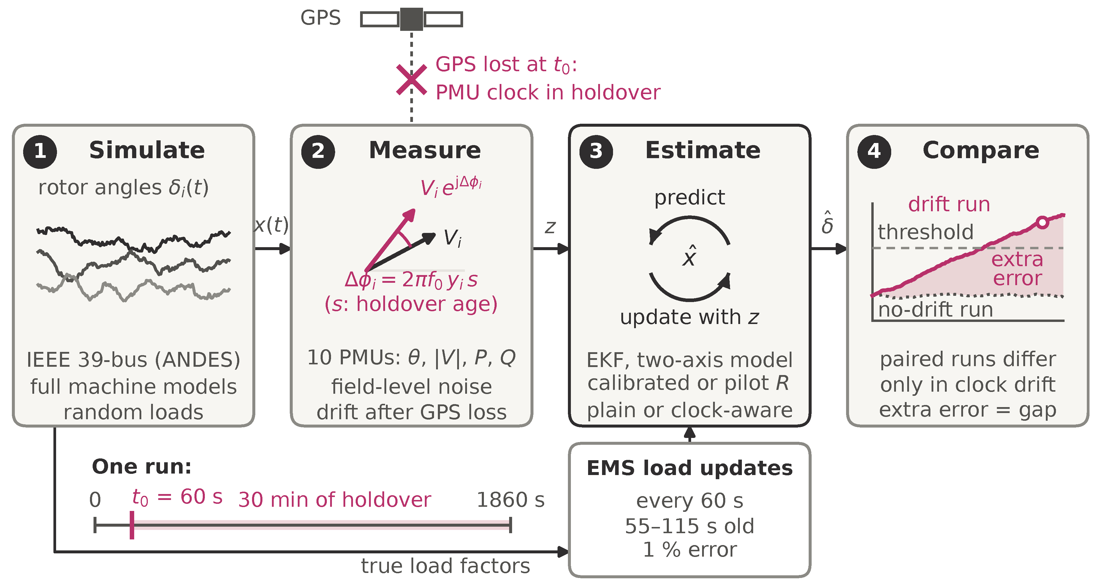
Figure 2.
IEEE 39-bus test system. A phasor measurement unit (PMU) sits at each of the ten generator terminal buses (30–39). Single-PMU outages are simulated at buses 30, 35 and 39 (highlighted); the machine at bus 39 represents the external system and carries 66% of the total inertia. The load step is applied at bus 15 and the three-phase fault at bus 16 (Section 2.9). Bus positions are schematic.
Figure 2.
IEEE 39-bus test system. A phasor measurement unit (PMU) sits at each of the ten generator terminal buses (30–39). Single-PMU outages are simulated at buses 30, 35 and 39 (highlighted); the machine at bus 39 represents the external system and carries 66% of the total inertia. The load step is applied at bus 15 and the three-phase fault at bus 16 (Section 2.9). Bus positions are schematic.
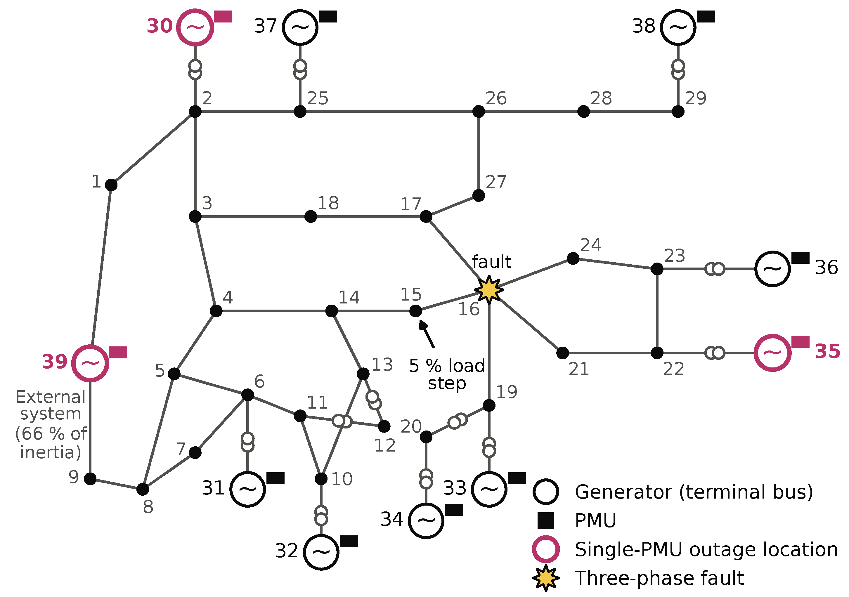
Figure 3.
Diagonal pass-through of a single drifting phasor measurement unit (PMU) against the filter’s ratio of angle to active-power variance, set B, plain extended Kalman filter (EKF), ten-machine centre-of-inertia (COI) frame. Lines: the closed form of Equation (7), with the angle, and Q variances of each tuning scaled together relative to P; the abscissa is the median over generators of . Filled dots: simulations at each tuning’s operating point (mean over 12 seeds, 1 min, compensated quartz). Open dots: simulations at and on angle, and Q (calibrated tuning, six seeds). Grey line: set A, whose pass-through does not depend on the weighting. Arrows: reduction from the calibrated to the pilot operating point.
Figure 3.
Diagonal pass-through of a single drifting phasor measurement unit (PMU) against the filter’s ratio of angle to active-power variance, set B, plain extended Kalman filter (EKF), ten-machine centre-of-inertia (COI) frame. Lines: the closed form of Equation (7), with the angle, and Q variances of each tuning scaled together relative to P; the abscissa is the median over generators of . Filled dots: simulations at each tuning’s operating point (mean over 12 seeds, 1 min, compensated quartz). Open dots: simulations at and on angle, and Q (calibrated tuning, six seeds). Grey line: set A, whose pass-through does not depend on the weighting. Arrows: reduction from the calibrated to the pilot operating point.
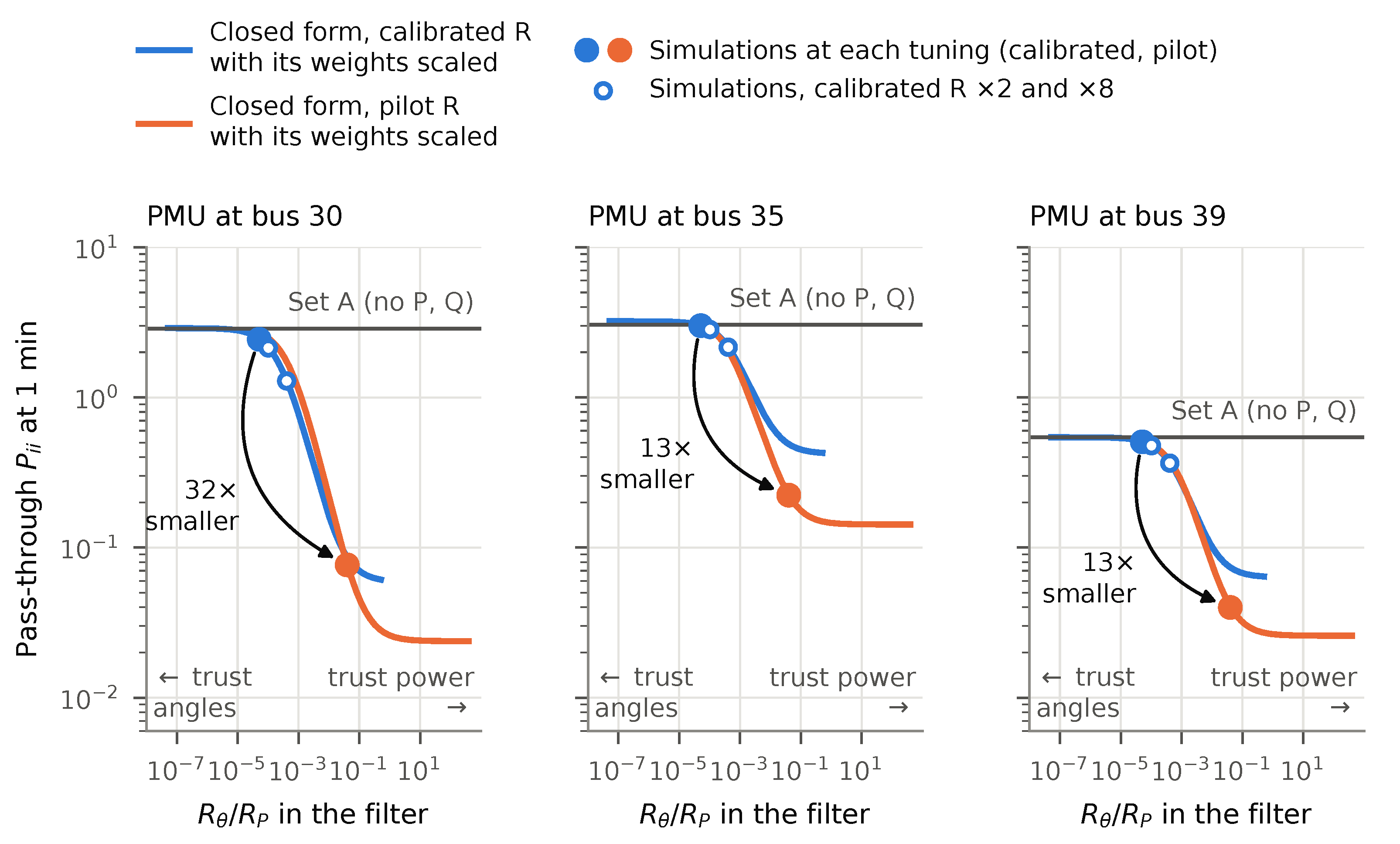
Figure 4.
Rotor-angle extra error (maximum over generators of the absolute centre-of-inertia error, drift run minus its paired no-drift run) against holdover age, set B, plain extended Kalman filter (EKF), compensated quartz, ten-machine frame, 12 seeds. Solid lines: root mean square (RMS) over seeds; bands: range over seeds. Dotted lines: the paired no-drift error (RMS over seeds, 60-s moving average) of the same tuning, which defines the self-referenced limit. Black line: the angle error of the drifting phasor measurement unit (PMU) itself; for all ten PMUs, the largest over PMUs, averaged over seeds. Dashed lines: fixed thresholds. Open circles: first crossing of 0.005 rad by the RMS extra error, labelled with its holdover age (Table 4).
Figure 4.
Rotor-angle extra error (maximum over generators of the absolute centre-of-inertia error, drift run minus its paired no-drift run) against holdover age, set B, plain extended Kalman filter (EKF), compensated quartz, ten-machine frame, 12 seeds. Solid lines: root mean square (RMS) over seeds; bands: range over seeds. Dotted lines: the paired no-drift error (RMS over seeds, 60-s moving average) of the same tuning, which defines the self-referenced limit. Black line: the angle error of the drifting phasor measurement unit (PMU) itself; for all ten PMUs, the largest over PMUs, averaged over seeds. Dashed lines: fixed thresholds. Open circles: first crossing of 0.005 rad by the RMS extra error, labelled with its holdover age (Table 4).
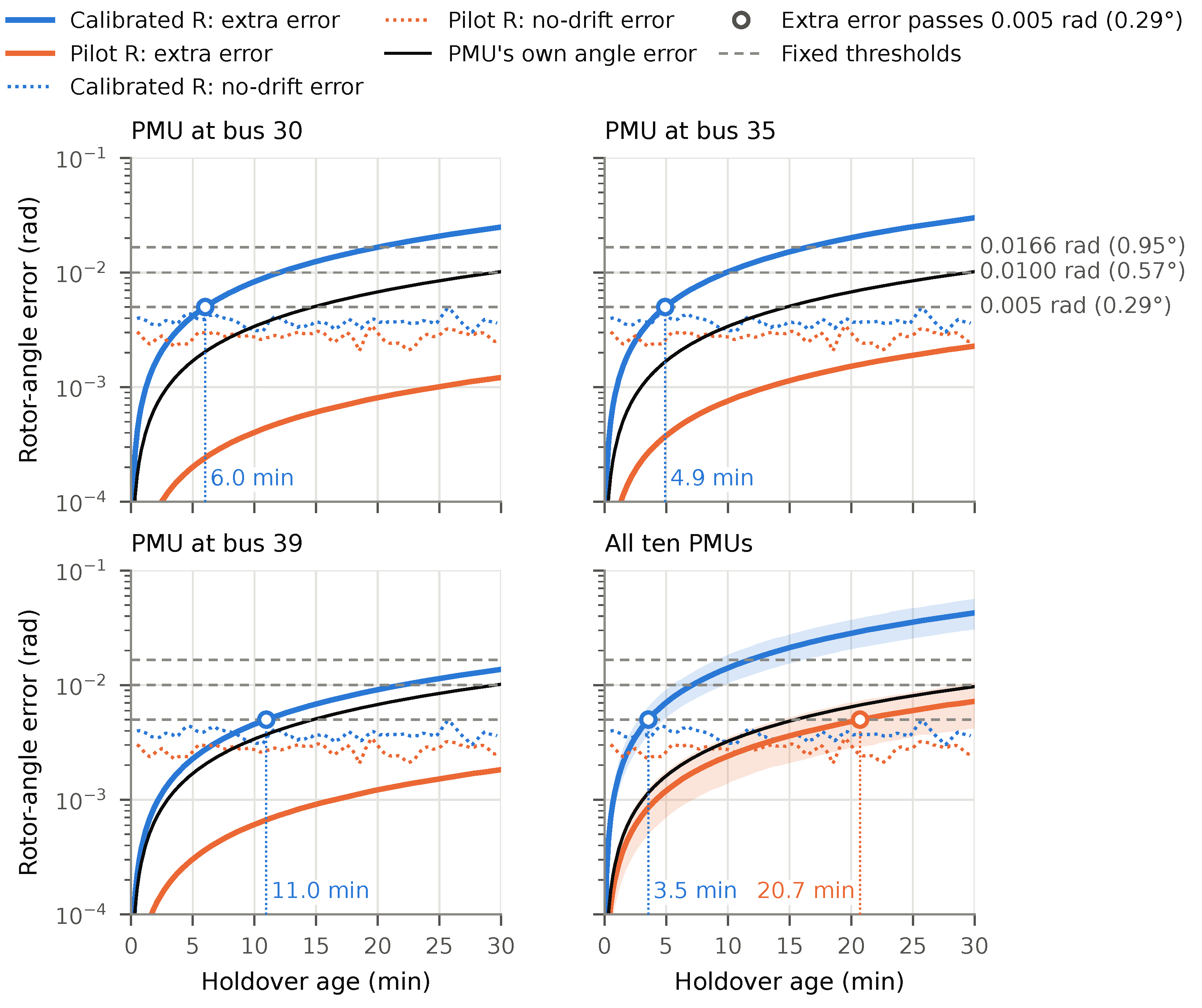
Figure 5.
Holdover age at which the rotor-angle extra error passes 0.005 rad (filled circles) and the self-referenced limit (open diamonds), set B, plain extended Kalman filter (EKF), compensated quartz, ten-machine frame, root mean square (RMS) over six seeds (seeds 1000–1005, also for the primary row). Left: calibrated R, phasor measurement unit (PMU) at bus 35. Right: pilot R, all ten PMUs. Each row changes one factor from the primary configuration. Triangles at the right edge: not crossed within 30 min. The cases were run at the calibrated tuning only.
Figure 5.
Holdover age at which the rotor-angle extra error passes 0.005 rad (filled circles) and the self-referenced limit (open diamonds), set B, plain extended Kalman filter (EKF), compensated quartz, ten-machine frame, root mean square (RMS) over six seeds (seeds 1000–1005, also for the primary row). Left: calibrated R, phasor measurement unit (PMU) at bus 35. Right: pilot R, all ten PMUs. Each row changes one factor from the primary configuration. Triangles at the right edge: not crossed within 30 min. The cases were run at the calibrated tuning only.
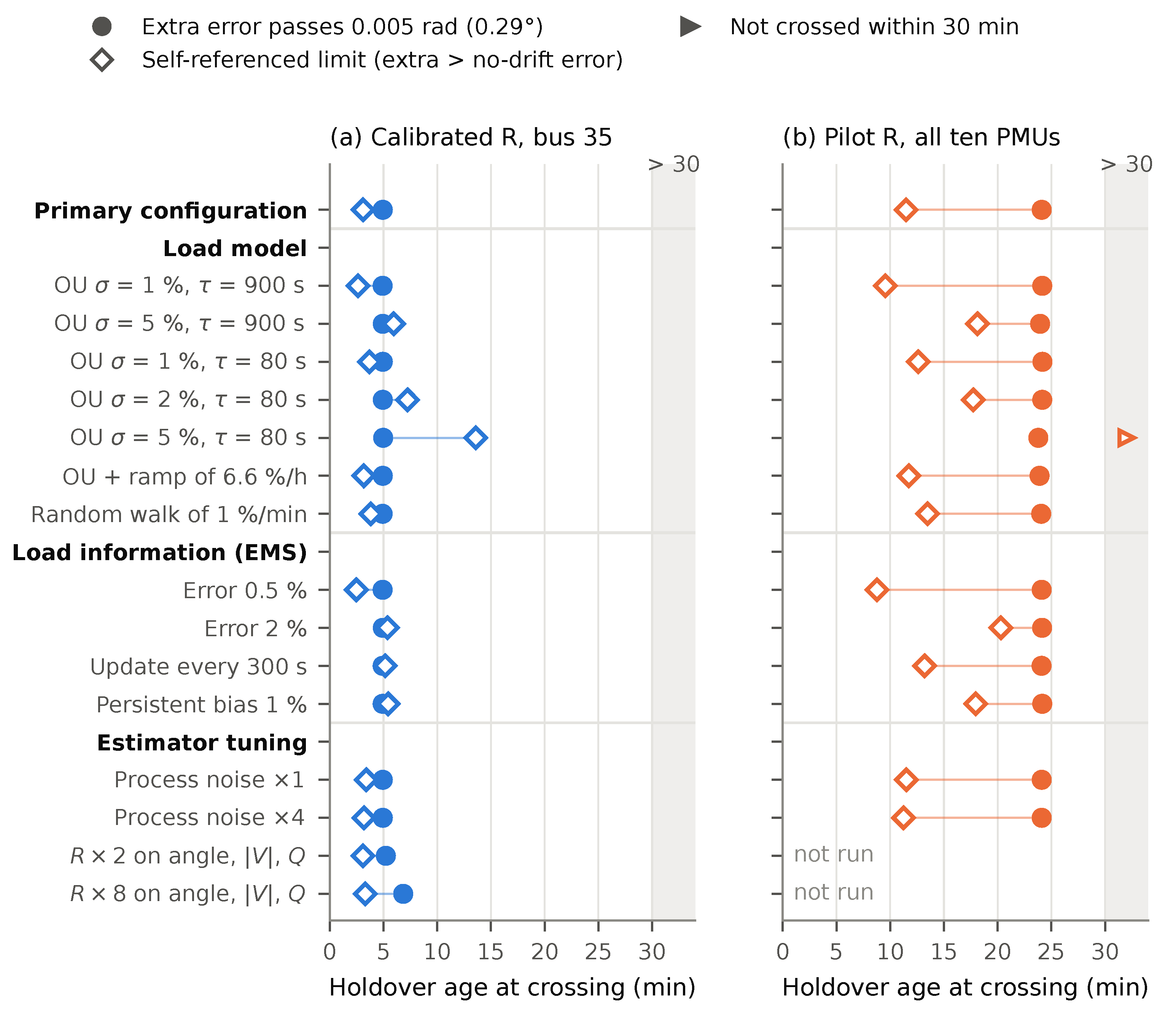
Figure 6.
Holdover time until an angle error of 0.005 rad (0.29°), by clock class, at each class’s upper rate. Squares: the angle error of the phasor measurement unit (PMU) itself. Circles: the rotor-angle extra error of a single drifting PMU at each tuning’s worst location, from Equation (8) with the closed-form maximum pass-through (extrapolated after the runs; values as in Table 5). Open markers lie beyond the clock’s measured record, shown by the grey bar, and assume a linear drift and an unchanged operating point. Shaded: the first 30 min, within which most recorded losses of the Global Positioning System (GPS) signal ended [2].
Figure 6.
Holdover time until an angle error of 0.005 rad (0.29°), by clock class, at each class’s upper rate. Squares: the angle error of the phasor measurement unit (PMU) itself. Circles: the rotor-angle extra error of a single drifting PMU at each tuning’s worst location, from Equation (8) with the closed-form maximum pass-through (extrapolated after the runs; values as in Table 5). Open markers lie beyond the clock’s measured record, shown by the grey bar, and assume a linear drift and an unchanged operating point. Shaded: the first 30 min, within which most recorded losses of the Global Positioning System (GPS) signal ended [2].
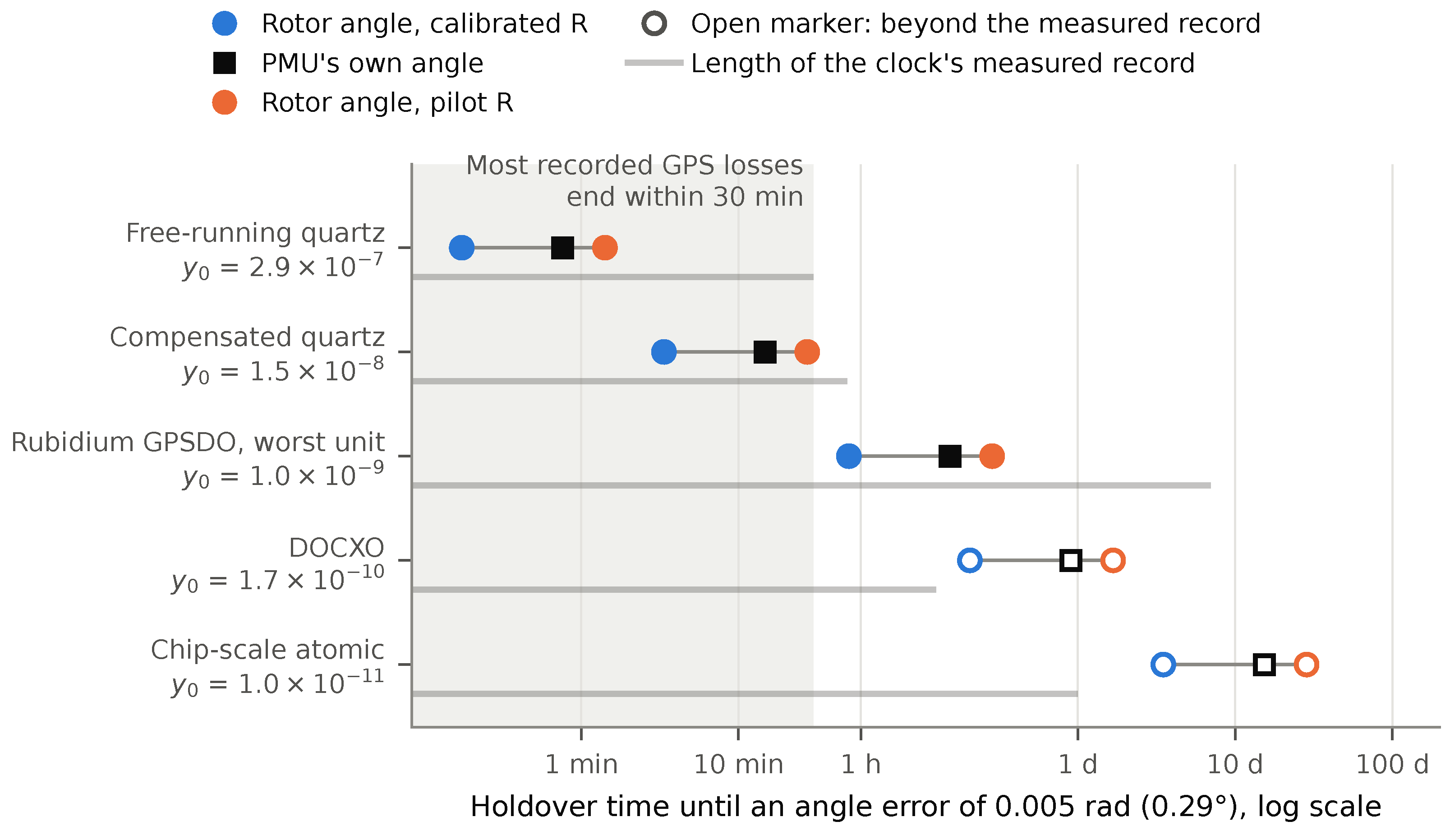
Table 1.
Closest prior studies of timing error in power-system state estimation.
| Study | Estimator and states | Timing treatment | Holdover time or clock class? |
|---|---|---|---|
| Yang et al. [11] | Static and dynamic network SE (bus voltages); IEEE 14–118 | Linear drift between re-synchronizations, estimated jointly | No; error vs. re-sync interval (seconds) |
| black!22blackTodescato et al. [14] | Kalman filter on a distribution network state; IEEE 123-node, EPFL feeder | Clock offset and skew states; re-sync every 1 s | No |
| black!22blackRisbud et al. [15] | Multi-period network SE | Time-varying spoofing offsets, estimated jointly | No |
| black!22blackPradhan et al. [17] | Linear KF, third-order generator model; WSCC 9-bus | Two step offsets (18°, 180°) at one PMU; detection | No |
| black!22blackSiamak et al. [18] | KF on generator model from angle-free measurements; IEEE 14-bus | Constant, ramp and oscillatory offsets; detection and correction | No |
| black!22blackPresent study | EKF, two-axis generator model, full ANDES reference simulation; IEEE 39-bus | Holdover drift of sourced clock classes; single-PMU and wide-area; plain and clock-aware; two measurement weightings | Yes; error vs. holdover age, closed-form pass-through, mapped to clock classes |
SE, state estimation; KF, Kalman filter; EKF, extended Kalman filter; WSCC, Western Systems Coordinating Council; EPFL, École Polytechnique Fédérale de Lausanne.
Table 2.
Clock classes. The phasor measurement unit (PMU) is disciplined by the Global Positioning System (GPS) until the outage (). Measured rows give a linear drift over the stated record. Specification rows (“spec”) are manufacturer bounds, not measurements of the tested units. Times are to 26.5 µs, the phase equivalent of 1% total vector error (TVE) at 60 Hz, from Equation (2).
Table 2.
Clock classes. The phasor measurement unit (PMU) is disciplined by the Global Positioning System (GPS) until the outage (). Measured rows give a linear drift over the stated record. Specification rows (“spec”) are manufacturer bounds, not measurements of the tested units. Times are to 26.5 µs, the phase equivalent of 1% total vector error (TVE) at 60 Hz, from Equation (2).
| Class | and a | Evidence and record | Time to 26.5 µs |
|---|---|---|---|
| Free-running quartz | –; a not reported | Three units, 30-min lab holdover [2] | 1.5–4.4 min |
| black!22blackCompensated quartz | –; a not reported | Derived from reported times to 1% TVE and larger thresholds [2,3] | 29–49 min |
| black!22blackDOCXO | One unit, 3-h lab test [3] | ≈43 h (linear, beyond the record) | |
| black!22blackDOCXO, spec | (measured) with aging 0.05–0.2 ppb/day | Data sheet [28]; production statistics [29] | 26–36 h |
| black!22blackChip-scale atomic | One unit, 24 h, lab temperature [4] | Not usable alone (31× beyond the record) | |
| black!22blackChip-scale atomic, spec | Temperature ( to 70 °C); aging /month, typical | Data sheet [30] | 14.5 h (worst temperature); 4.6 d (aging only) |
| black!22blackRubidium GPSDO | to | Three units, one week of holdover [31] | ≈7 h to ≈100 d |
| black!22blackRubidium, spec | Temperature –; aging –/month | Data sheet [32] | 2.9–5.6 d (worst temperature); 14–19 d (aging only) |
| black!22blackOptical (iodine) | Three clocks, 20 days at sea [33] | Centuries |
DOCXO, double-oven crystal oscillator; GPSDO, GPS-disciplined oscillator; ppb, parts per billion.
Table 3.
Pass-through of a single drifting phasor measurement unit (PMU), plain extended Kalman filter (EKF), compensated quartz, 1 min into holdover. : the drifting PMU’s own machine, measured as the mean over 12 seeds, with the closed-form value of Equation (7), logged before the runs, in parentheses (ten-machine centre-of-inertia frame). Spillover: the largest over the other machines, in the ten- and nine-machine frames. Set A is identical at both tunings to the digits shown; its two tunings’ are given as a range.
Table 3.
Pass-through of a single drifting phasor measurement unit (PMU), plain extended Kalman filter (EKF), compensated quartz, 1 min into holdover. : the drifting PMU’s own machine, measured as the mean over 12 seeds, with the closed-form value of Equation (7), logged before the runs, in parentheses (ten-machine centre-of-inertia frame). Spillover: the largest over the other machines, in the ten- and nine-machine frames. Set A is identical at both tunings to the digits shown; its two tunings’ are given as a range.
| Configuration | Bus 30 | Bus 35 | Bus 39 |
|---|---|---|---|
| Set B, calibrated R: | 2.437 (2.460) | 3.005 (3.012) | 0.506 (0.510) |
| spillover, 10/9 machines | 1.29 / 1.44 | 1.17 / 1.28 | 1.34 / 0.35 |
| black!22blackSet B, pilot R: | 0.0766 (0.0772) | 0.2233 (0.2240) | 0.0399 (0.0405) |
| spillover, 10/9 machines | 0.12 / 0.12 | 0.22 / 0.19 | 0.18 / 0.10 |
| black!22blackSet A, either R: | 2.86–2.87 (2.896) | 3.04–3.05 (3.055) | 0.542–0.543 (0.547) |
| spillover, 10/9 machines | 1.99 / 2.18 | 1.18 / 1.29 | 1.52 / 0.46 |
| black!22blackSet B, calibrated/pilot | 31.8 | 13.5 | 12.7 |
Table 4.
Holdover age (min) at which the rotor-angle extra error first passes each fixed threshold, and the self-referenced limit. Primary configuration: set B, plain extended Kalman filter (EKF), ten-machine centre-of-inertia (COI) frame, Ornstein–Uhlenbeck (OU) load model with and s, 12 seeds. Each value is for the root mean square (RMS) over seeds; the range over individual seeds is given in parentheses where the outage set or the definition makes it vary: for all ten phasor measurement units (PMUs), whose rates are drawn per seed, and for the self-referenced limit, which compares each seed with its own no-drift error. Single-PMU fixed-threshold crossings vary by at most 0.6 min between seeds. : not crossed within the simulated 30 min (censored). For comparison, the PMU’s own angle error at the compensated class’s upper bound reaches 0.005 rad at 14.7 min and 0.0100 rad at 29.5 min.
Table 4.
Holdover age (min) at which the rotor-angle extra error first passes each fixed threshold, and the self-referenced limit. Primary configuration: set B, plain extended Kalman filter (EKF), ten-machine centre-of-inertia (COI) frame, Ornstein–Uhlenbeck (OU) load model with and s, 12 seeds. Each value is for the root mean square (RMS) over seeds; the range over individual seeds is given in parentheses where the outage set or the definition makes it vary: for all ten phasor measurement units (PMUs), whose rates are drawn per seed, and for the self-referenced limit, which compares each seed with its own no-drift error. Single-PMU fixed-threshold crossings vary by at most 0.6 min between seeds. : not crossed within the simulated 30 min (censored). For comparison, the PMU’s own angle error at the compensated class’s upper bound reaches 0.005 rad at 14.7 min and 0.0100 rad at 29.5 min.
| Outage | rad (0.29°) | rad (0.57°) | rad (0.95°) | Self-referenced |
|---|---|---|---|---|
| Calibrated R, compensated quartz | ||||
| Bus 30 | 6.0 | 12.0 | 20.0 | 4.0 (2.1–5.3) |
| Bus 35 | 4.9 | 9.8 | 16.4 | 3.3 (1.7–4.4) |
| Bus 39 | 11.0 | 21.9 | 7.2 (3.7–8.6) | |
| All ten | 3.5 (2.8–4.8) | 7.1 (5.5–9.7) | 11.8 (9.1–16.1) | 2.4 (1.1–3.1) |
| black!22black5@lCalibrated R, free-running quartz | ||||
| Bus 30 | 0.3 | 0.6 | 1.1 | 0.2 (0.1–0.3) |
| Bus 35 | 0.3 | 0.5 | 0.9 | 0.2 (0.1–0.3) |
| Bus 39 | 0.6 | 1.1 | 1.9 | 0.4 (0.2–0.6) |
| All ten | 0.2 (0.1–0.3) | 0.4 (0.3–0.6) | 0.7 (0.5–1.0) | 0.1 (0.1–0.3) |
| black!22black5@lPilot R, compensated quartz | ||||
| Bus 30 | (25.4; 11 ) | |||
| Bus 35 | (14.5–27.3; 1 ) | |||
| Bus 39 | (16.5–29.6; 3 ) | |||
| All ten | 20.7 (14.4–27.3; 4 ) | (28.9; 11 ) | 9.3 (6.0–19.1) | |
| black!22black5@lPilot R, free-running quartz | ||||
| Bus 30 | 6.4 | 12.8 | 21.2 | 3.2 (1.8–5.0) |
| Bus 35 | 3.4 | 6.8 | 11.2 | 1.7 (1.2–2.5) |
| Bus 39 | 4.3 | 8.4 | 14.0 | 2.1 (1.4–3.1) |
| All ten | 1.6 (1.2–3.9) | 3.2 (2.3–8.0) | 5.3 (3.9–13.1) | 0.8 (0.4–1.4) |
Table 5.
Holdover of a single phasor measurement unit (PMU) until the rotor-angle extra error reaches 0.005 and 0.0100 rad, extrapolated after the runs with Equation (8) at each class’s upper rate. is the closed-form maximum over generators and over all ten PMU locations, in either centre-of-inertia frame: 4.39 with the calibrated R (PMU at bus 37) and 0.54 with the pilot R (bus 38). Times longer than the clock’s own measured record (marked †) assume that its drift stays linear; times of hours or more also assume that the operating point does not change, which the linearization does not cover. They rank the classes and are not guarantees.
Table 5.
Holdover of a single phasor measurement unit (PMU) until the rotor-angle extra error reaches 0.005 and 0.0100 rad, extrapolated after the runs with Equation (8) at each class’s upper rate. is the closed-form maximum over generators and over all ten PMU locations, in either centre-of-inertia frame: 4.39 with the calibrated R (PMU at bus 37) and 0.54 with the pilot R (bus 38). Times longer than the clock’s own measured record (marked †) assume that its drift stays linear; times of hours or more also assume that the operating point does not change, which the linearization does not cover. They rank the classes and are not guarantees.
| Calibrated R | Pilot R | |||
|---|---|---|---|---|
| Clock class () | 0.005 rad (0.29°) | 0.0100 rad (0.57°) | 0.005 rad (0.29°) | 0.0100 rad (0.57°) |
| Free-running quartz () | 10 s | 21 s | 85 s | 2.8 min |
| Compensated quartz () | 3.4 min | 6.7 min | 27 min | 55 min† |
| Rubidium GPSDO, worst unit () | 50 min | 101 min | 6.8 h | 14 h |
| DOCXO () | 4.9 h† | 9.9 h† | 40 h† | 3.4 d† |
| Chip-scale atomic () | 3.5 d† | 7.0 d† | 28 d† | 57 d† |
DOCXO, double-oven crystal oscillator; GPSDO, oscillator disciplined by the Global Positioning System.
Disclaimer/Publisher’s Note: The statements, opinions and data contained in all publications are solely those of the individual author(s) and contributor(s) and not of MDPI and/or the editor(s). MDPI and/or the editor(s) disclaim responsibility for any injury to people or property resulting from any ideas, methods, instructions or products referred to in the content. |
© 2026 by the authors. Licensee MDPI, Basel, Switzerland. This article is an open access article distributed under the terms and conditions of the Creative Commons Attribution (CC BY) license (http://creativecommons.org/licenses/by/4.0/).
Copyright: This open access article is published under a Creative Commons CC BY 4.0 license, which permit the free download, distribution, and reuse, provided that the author and preprint are cited in any reuse.