

Submitted:
13 November 2026
Posted:
17 November 2026
You are already at the latest version
Abstract
Single-phase photovoltaic inverters are a leading cause of overvoltage on long low-voltage (LV) feeders. A residential battery operated only for its owner, the prosumer, is usually full before the midday voltage peak and gives the feeder little relief. This paper develops the voltage-service flexumer (VSF), a prosumer battery operated for both self-consumption and voltage support, with a controller built from three components with proven properties: a ridge estimator of phase-resolved voltage sensitivities, with sign restrictions derived from the linearized four-wire power-flow equations, which is the projection of ordinary ridge regression onto a convex cone; a split-conformal safety margin with a joint, distribution-free coverage guarantee; and a state-of-charge-weighted linear program whose dual variables act as voltage shadow prices, complemented by an export-headroom reserve and a voltage-safe discharge rule. On a real unbalanced 20/0.4 kV network with 231 users and 58 prosumers, where the voltage exceeds 253 V in 124 of 672 intervals, the estimator reaches an out-of-sample error of 0.32 V, half that of a neural network, and the 2.0 V margin attains 95.6% coverage. With identical 10 kWh batteries, the prosumer leaves 74 overvoltage intervals, whereas the VSF removes all of them, without curtailment and without reducing the owners' self-consumption.
Keywords:
flexumer
; battery energy storage
; overvoltage
; voltage rise
; low-voltage networks
; physics-constrained learning
; regression
1. Introduction
1.1. From Prosumers to Flexumers
The role of the residential electricity user has changed twice in little more than a decade. The first change produced the prosumer, a household that generates electricity, mostly from rooftop photovoltaics (PV), covers part of its own demand and exports the remainder [1,2]. The second change, now well under way, adds a battery and an energy management system. Sioshansi and co-authors named this user the prosumager [3], a prosumer that also stores and manages energy. Its priority, however, remains its own bill. A further term, flexumer, has been used for prosumers who apply their flexibility to market, network or system services [4]. The two terms are not interchangeable. The presence of a battery tells nothing about whether the battery is operated in the interest of the network, and European legislation, while granting active customers the right to offer flexibility [5], does not prescribe how a residential battery should serve the LV feeder it is connected to.
1.2. The Overvoltage Problem in Unbalanced LV Networks with Prosumers
The network operation most needed in many LV systems today is voltage support. Long overhead feeders with high resistance-to-reactance (R/X) ratios, a high share of single-phase PV inverters and a busbar voltage that is already elevated at midday produce voltage rise well before thermal limits are reached [6,7,8,9]. Single-phase connection aggravates the problem in two ways. First, the return current flows through the neutral conductor, so the voltage rise seen by the injecting phase is governed by the sum of the phase and neutral resistances. Second, the neutral potential is displaced, and the voltages of the other two phases change as well, in a direction that depends on the network [10,11]. The conventional remedies are reactive power control Q(U), active power curtailment P(U), on-load tap changers at the secondary substation and reinforcement [12,13,14,15,16]. Each has a known weakness. Reactive power is ineffective when R/X is high, curtailment discards renewable energy, tap changers act on all phases at once and reinforcement is slow and costly.
1.3. Storage as a Remedy
Batteries absorb the surplus where it is produced and are therefore well suited to overvoltage mitigation [17,18,19,20]. The difficulty lies in the operating rule. A battery that serves self-consumption starts charging with the first surplus of the morning, is often full before the voltage peak around noon and can do nothing when the network needs it most [17]. Turning a prosumager into a useful flexumer requires answers to three questions that a distribution system operator (DSO) rarely can answer for its LV networks:
- Which battery, on which phase, lowers which node voltage, and by how much?
- How much can that estimate be trusted, and what safety margin follows from it?
- How much energy must each battery keep free for the rest of the day, and how much can it still store for its owner?
1.4. Research Questions and Contributions
This paper argues that all three questions can be answered from data that DSOs already collect, using learning methods whose mathematical properties are known and verifiable. The investigation is organised around four research questions:
- RQ1. Can phase-resolved voltage sensitivities be learned from smart-meter data in a way that is both accurate and consistent with the physics of a four-wire network?
- RQ2. Can the error of such a learned model be bounded by a margin with a stated reliability that does not depend on distributional assumptions?
- RQ3. Can a controller built on these two components eliminate overvoltage with residential batteries while preserving the owners’ self-consumption and avoiding curtailment?
- RQ4. Which elements of the controller are necessary, and how sensitive is the result to its parameters and to the battery size?
The contributions are the following:
- The voltage-service flexumer is defined as an operating mode of a prosumer battery with an explicit network objective, and it is compared, on the same hardware, with the prosumager and with P(U) curtailment.
- A physics-constrained ridge (PC-ridge) estimator of phase-resolved sensitivities is derived. The sign restrictions follow from the linearized four-wire power-flow equations (Proposition 1). The estimator is unique and equals the metric projection of ordinary ridge regression onto a convex cone, which implies that it is never farther from a physically consistent truth than ridge regression itself (Propositions 2 and 3).
- A split-conformal safety margin is constructed for the incremental prediction used by the controller. Defining the score as a maximum over node-phases yields a joint coverage guarantee (Theorem 1 and Corollary 1).
- A VSF controller is built from a state-of-charge (SoC)-weighted linear program (LP), an export-headroom reserve and a voltage-safe discharge rule. The LP dual variables are interpreted as voltage shadow prices, which explain how the controller selects batteries (Proposition 4). The reserve and the discharge rule come with an invariance property and a convergence result (Propositions 5 and 6).
- The approach is evaluated on a real unbalanced LV network in north-eastern Romania, with a separation of training, calibration and test days, an ablation study and sensitivity analyses that link every result to an element of the algorithm.
1.5. Paper Structure
Section 2 reviews related work and positions the contribution in a comparison table. Section 3 describes the network and the data. Section 4 presents the mathematical formulation, theoretical methodology and the proposed algorithm. Section 5 defines experimental design. Section 6 reports the results, organized according to the research questions. Section 7 discussion and limitations, and Section 8 the approach conclusions.
2. Related Work and Research Gap
2.1. Voltage Rise Mitigation in LV Networks
The physics of voltage rise in distribution feeders with embedded generation has been understood for two decades [6,7]. Experience from high-PV regions such as Germany showed that voltage, not thermal loading, limits the hosting capacity of rural LV feeders [8,14]. Reactive power control by PV inverters was proposed early as a local, communication-free remedy [12]. Its effectiveness is limited by the high R/X ratio of LV conductors, and the additional reactive current increases the losses. Active power curtailment is always effective but sacrifices energy, and coordinated schemes have been designed to distribute the curtailment fairly among prosumers [13]. On-load tap changers at the secondary substation, controlled with or without remote monitoring, act on the busbar voltage and cannot correct phase-specific deviations [15]. Comparative reviews conclude that no single measure suffices at high penetration and that combinations are necessary [16]. Dynamic operating envelopes limit the export of each prosumer according to the network state [24], which is again a form of curtailment when the limit is binding.
2.2. Batteries for Voltage Support
Von Appen et al. compared local strategies for PV-storage systems and showed that self-consumption-oriented operation does little for voltage, because the batteries are full at midday [17]. Marra et al. proposed a decentralised charging strategy for residential feeders that charges in proportion to the voltage [18]. Coordinated approaches use communication between storage units. Wang et al. applied a consensus algorithm to distribute the voltage regulation effort among distributed storage units [19], and Zeraati et al. added SoC balancing to distributed battery control for feeders with high PV penetration [20]. These approaches assume a model of the network, typically balanced, and do not quantify the uncertainty of the control law. In the authors’ previous work, the location of storage in four-wire LV networks was optimised for loss reduction [22], and battery storage was combined with tap changers and Q(U) control in a four-wire model [23]. Both studies relied on a full network model.
2.3. Data-Driven Voltage Sensitivities and Physics-Informed Learning
Model-based sensitivity coefficients for unbalanced radial networks can be computed efficiently when the network model is known [25], and linear approximations of the power-flow solution are well founded [26]. For LV networks, however, the model is often incomplete or outdated. Measurement-based estimation of sensitivities from synchronised measurements has been demonstrated in laboratory and field conditions [27,28]. Such estimators face a specific statistical difficulty: on a sunny day, all PV systems produce together, the regressors are strongly collinear and individual coefficients are poorly identified. Physics-informed learning addresses such situations by embedding prior knowledge into the model [29], and in power systems it has mostly been used with neural networks [30]. Constraining a linear estimator by the sign structure implied by the power-flow equations is a simpler and more transparent way of injecting physics, and its statistical consequences can be stated exactly. Deep reinforcement learning has also been applied to voltage control [31,32], but its training requires large amounts of data or a simulator, and its safety guarantees are difficult to formulate.
2.4. Uncertainty Quantification for Safe Control
Conformal prediction converts any point predictor into a set predictor with a finite-sample, distribution-free coverage guarantee under exchangeability [33,34,35]. Extensions handle non-exchangeable and time-series data [36,37]. In robotics, conformal regions have been used to certify the safety of planned trajectories [38]. In power systems, conformal prediction has been applied mainly to forecasting. Its use to calibrate the safety margin of a voltage controller, in particular for the error of an incremental sensitivity model and with a joint guarantee over all node-phases, has not been reported to the best of the authors’ knowledge.
2.5. Research Gap and Positioning
Table 1 compares representative approaches according to eight criteria that together characterize a battery-based voltage control suitable for unbalanced LV networks with limited model knowledge. A tick means that the criterion is an explicit part of the approach (◐ means that it is partly addressed, a dash means that it is not addressed.
The criteria indicated in Table 1 are the following: C1, phase-resolved representation of an unbalanced four-wire network; C2, sensitivities or control law learned from operational data; C3, physical consistency of the learned or computed model guaranteed by construction; C4, safety margin with a stated, distribution-free reliability; C5, batteries coordinated explicitly for voltage support; C6, owners’ self-consumption explicitly preserved; C7, PV curtailment avoided; C8, a mechanism that prevents batteries from saturating before the voltage peak.
Two observations follow from Table 1. The storage-based approaches (C5) assume a network model and provide no reliability statement for the control (C2–C4). The data-driven approaches (C2), for their part, either do not control storage or give no guarantees. None combines learning from data, physical consistency and a calibrated margin with storage control that keeps the owners’ benefit and avoids curtailment. The approach proposed in this paper fills this gap, and the following sections show that each criterion in Table 1 corresponds to a concrete, analyzable element of the algorithm.
3. Network and Data
3.1. Test Network
The case study is a suburban LV network in north-eastern Romania, operated by the regional distribution system operator. The network is supplied by a 20/0.4 kV, 250 kVA secondary substation and consists of four overhead feeders with spans of approximately 40 m. It supplies 231 users: 173 consumers and 58 prosumers connected under the national technical rules for prosumers [39]. The main characteristics are summarized in Table 2. The prosumer inverters are rated at 10 kVA (52 units), 16 kVA (3), 6 kVA (2) and 5 kVA (1). Fifty-four prosumers are single-phase (14 on phase A, 22 on phase B, 18 on phase C) and four are three-phase. Forty-four prosumers exported energy during the period analyzed. They are concentrated on feeders 1 and 2, which host 31 and 25 prosumers and exported 771 kWh and 507 kWh, respectively.
3.2. Data
The data set covers seven consecutive summer days with a 15-min resolution, i.e., 672 intervals, numbered here as days 1–7. For each user and each phase, the active power and reactive power come from smart meters. Positive values denote consumption and negative values denote export (load convention). The phase-to-neutral voltage magnitudes at the LV busbar and at the 121 pole nodes were obtained by the DSO from load-flow simulations of the network model in DIgSILENT PowerFactory, driven by the measured profiles. Each user is mapped to the pole node and to the phase it is connected to.
Figure 1 places the users of this network in the sequence of roles discussed in Section 1. The mean daily profile in Figure 2 shows the structure of the problem. The four roles differ in the resources they own and in whose interest the battery is operated. The busbar voltage alone rises from about 240 V at night to about 246 V around noon, owing to the medium-voltage network and the transformer. The prosumers add up to 10.9 V on top of it. During the intervals with overvoltage, the busbar voltage averages 248.6 V, so the remaining margin to 253 V is small and is consumed by local injections. Feeder 1 is responsible for all 124 overvoltage intervals, and feeder 2 also exceeds the limit in 14 of them. The violations occur on six of the seven days.
The overvoltages are distributed unevenly over the phases. Of the 2622 node-phase-intervals above 253 V, 1762 occur on phase A, 671 on phase C and only 189 on phase B, although phase B hosts the most prosumers. Local injections alone cannot explain this pattern. Coupling between the phases, through the neutral conductor and the network, must also play a role, which a model that ignores the phases cannot represent.
4. Mathematical Formulation
The complete workflow is shown in Figure 3. Days 1–4 are used to learn the sensitivities, day 5 to calibrate the conformal margin and days 6–7 are kept for out-of-sample testing. The export-headroom reserve uses days 1–5, so days 6–7 are never seen by any component of the method.
4.1. Notation
The main symbols are listed in Table 3. Vectors are bold, denotes a phase and h the interval length.
4.2. Linearized Four-Wire Model and Sign Structure
Consider a radial four-wire feeder in which each branch has a phase impedance and a neutral impedance . In the idealised model analysed here, mutual coupling is neglected and the neutral is earthed only at the substation. Let be the set of branches on the path from node to the substation, and let be the angle of phase . The phase-to-neutral voltages are linearised around the nominal magnitude . An injection of active power at node on phase , at unity power factor, produces the current , which flows towards the substation in the phase conductor and returns in the neutral.
The linearization follows the reasoning of the DistFlow equations [40], extended here to the four-wire case.
Proposition 1 (sign structure of the sensitivities). In the idealised linearised model, the sensitivity of the voltage magnitude at node on phase to an active power injection at node on phase is
with . The own-phase sensitivity is non-negative and grows with the length of the shared path. The cross-phase sensitivity has no fixed sign.
Proof. On each branch of the shared path, the phase conductor carries the current towards the substation and the neutral carries it back. The phase potential at node therefore rises by relative to the substation, and the neutral potential falls by . The phase-to-neutral voltage of phase changes by , and that of another phase by , since only the neutral potential changes for it. To first order, the change of a magnitude equals the projection of the complex change on the direction of the voltage. Substituting gives for the own phase and for the others. The first expression is a sum of positive terms over a set that grows with the shared path. The second equals , whose sign depends on and on the ratio . □
Proposition 1 has two consequences for learning. With the load convention, an injection is a negative , so the own-phase coefficients of active power must satisfy
This restriction is robust: it holds for any positive resistance and does not require their values. For the cross-phase coefficients, the idealized model gives no fixed sign, and mutual coupling, multiple earthing of the neutral and the operating point add further terms of either sign. These coefficients are therefore left unrestricted and learned from the data. The magnitude implied by Equation (1) also serves as a plausibility check. For a typical 3 × 95 + 50 mm2 aluminum bundled conductor, /km, so one kilometre of shared path gives about V per kW injected.
4.3. Physics-Constrained Ridge Estimator
4.3.1. Model and Estimator
The voltage rise is modelled as
where is the vector of regressors standardised on the training set, the intercept and the residual. Using the rise above the busbar voltage, rather than the absolute voltage, removes the effect of the medium-voltage network, which the LV resources cannot control. The 120 regressors are the active and reactive powers of the 48 prosumer channels that were active in the data and the aggregated active and reactive powers of the consumers of each feeder and phase. Each output column is estimated by a ridge regression [41] subject to the sign restrictions:
where is the centred output is recovered as the training mean of and contains the pairs of an active power regressor on phase and an output on the same phase. Since standardisation divides by a positive scale, the sign restriction on is equivalent to Equation (2).
Proposition 2 (existence, uniqueness and optimality conditions). For , problem (4) has a unique solution. A vector is the solution if and only if there exists , with for , such that
Proof. The objective is a quadratic function with Hessian , hence strictly convex. The feasible set is a non-empty (it contains ), closed and convex polyhedral cone. A strictly convex, coercive function attains a unique minimum on a non-empty closed convex set. The constraints are affine, so Slater’s condition is not needed and the Karush–Kuhn–Tucker conditions (5) are necessary and sufficient [42]. □
The conditions (5) give an interpretation of the constrained coefficients. A coefficient is either free, in which case it satisfies the ridge normal equation, or it is held at zero by a non-negative multiplier . In the latter case, the data alone would have pushed it towards a positive, physically impossible value.
4.3.2. Projection Property
Let and let be the unconstrained ridge solution. Expanding the objective of (4) gives
so, the PC-ridge estimate is the projection of the ridge estimate onto the cone in the metric induced by :
Proposition 3 (the constraint never moves the estimate away from a consistent truth). Let be any coefficient vector that satisfies the physical sign restrictions, for instance the true sensitivity. Then
Proof. The metric projection onto a closed convex set in a Hilbert space is firmly non-expansive [43]. In particular, for any point of the set, , because . Applying this with , the metric induced by and Equation (7) gives (8). □
Proposition 3 is deterministic: it holds for every data set, not only on average. If the physical prior is correct, imposing it can only bring the estimate closer to the truth, in the norm that weighs each direction by its information content . The improvement is largest in the directions that the data identify poorly, which are exactly the directions created by the collinearity of synchronous PV profiles. The regularisation parameter is selected by leave-one-day-out cross-validation on the four training days [44]. Problem (4) is a bounded-variable least-squares problem [45] and is solved independently for each of the 363 outputs.
4.4. Conformal Safety Margin for the Incremental Model
4.4.1. Incremental Prediction
The controller does not predict voltages from scratch. It starts with the current voltages and predicts the effect of a change of the controllable injections:
The intercept and the slowly varying part of the error cancel in the difference, so the incremental prediction is more accurate than a prediction of the absolute voltage. Its remaining error comes from the inexact sensitivities and from the nonlinearity of the power flow.
4.4.2. Joint Score and Margin
For pairs of intervals of the calibration day with , the observed increments of regressors and voltage rises are compared with the prediction. The score is the largest under-prediction over the monitored node-phases:
where is the set of node-phases whose voltage exceeds a monitoring threshold in either interval. Here intervals (2 h), the pairs are taken between 06:00 and 20:00 and the monitoring threshold is 248 V. With the calibration scores sorted in increasing order, the margin at level is
Theorem 1 (joint distribution-free coverage). Let the calibration scores and the score of a new increment be exchangeable. Then
for any joint distribution of the data.
Proof. By exchangeability, the rank of among the scores is uniformly distributed on , with ties broken at random. The event requires that be among the largest scores, which has probability at most [33,34]. Because the score is the maximum over node-phases, the event is the intersection of the events for all node-phases, which proves the joint statement. □
Corollary 1 (probabilistic voltage guarantee). If a control action satisfies for all monitored , and the score of the realised increment is exchangeable with the calibration scores, then all monitored voltages after the action satisfy simultaneously with probability at least .
Proof. The realised voltage is with . On the event of Theorem 1, for every . □
Two remarks qualify for these results. First, successive 15-min increments are not exactly exchanging, so the guarantee is approximate. For this reason, the empirical coverage is verified on scores computed in the same way on the test days [36,37]. Second, the calibration increments are natural changes of the network state, whereas the control acts on a subset of channels. The margin is therefore validated in Section 6 both through the coverage on test days and through the voltages obtained under control.
4.5. Voltage-Service Flexumer Controller
4.5.1. Prosumager Reference Rule
The prosumager charges with all the surplus it can absorb and discharges only to its own demand:
where is the exported power of channel , and the power and upper energy limits and the charging efficiency.
4.5.2. SoC-Weighted Absorption Problem
Let be the operating limit and the set of node-phases within 5 V of it. Whenever at least one measured voltage exceeds , the VSF controller solves
where is the sensitivity of node-phase to the active power of channel , which is non-positive on the own phase by construction (Section 4.3), and are slack variables penalised by a large constant . Unlike the prosumager rule, the bound (16) does not contain the own export: a VSF may absorb power from the network at a node where the voltage is high, which lowers that voltage exactly as absorbing local surplus does. In this sense, the VSF absorbs the surplus of its neighbourhood. The weights are
The weight is the derivative of the barrier function , which tends to infinity as the battery approaches its upper limit. Problem (14)–(16) can thus be read as one step of a linearised minimisation of under the voltage constraints: the controller prefers batteries far from saturation and uses a nearly full battery only when no other can help.
Proposition 4 (feasibility, duality and battery selection). For any , problem (14)–(16) is feasible and has an optimal solution. Let be the optimal dual variables of the voltage constraints (15) and those of the upper bounds (16). Then and, for every channel,
Consequently, a channel charges () only if its weighted voltage-reduction value is at least its cost , with equality if it is not at its upper bound. When a single voltage constraint is binding, the optimal solution charges the channels in increasing order of the ratio until the constraint is met.
Proof. The point , is feasible. The objective is bounded below by zero on the feasible set, so an optimal solution exists [46]. The dual constraint associated with is . The dual constraint associated with and the complementary slackness condition give (18). With a single binding constraint, the problem reduces to a continuous knapsack problem whose optimal solution is greedy in the cost-to-effect ratio. □
Proposition 4 explains the behaviour of the controller and gives the dual variables a physical meaning. The multiplier is the marginal cost of lowering the voltage of node-phase by 1 V, i.e., a voltage shadow price. It increases when the batteries that can help become fuller, since their weights grow, and it reaches only when the constraint cannot be met. The number of LP solutions with is therefore a direct measure of the saturation of the storage resource.
4.5.3. Export-Headroom Reserve and Self-Consumption Charging
A VSF should also store its own surplus for the evening, but not so much that it cannot provide the voltage service later in the day. For each battery and each time of day , the remaining own export until midnight is computed on each of the days available before the test, and its maximum is kept:
After problem (14)–(16) has been solved, the self-consumption charging is obtained from a second LP:
The first term in (21) restricts self-consumption charging to the battery’s own surplus, the second to its power and energy limits and the third to the headroom above the reserve.
Proposition 5 (headroom invariance). Let and consider a day whose remaining own export curve of battery is dominated, at every time of day, by the maximum in (19). Assume that the reserve is satisfied at the start of the day. Then self-consumption charging never reduces the free capacity of battery below its remaining own export for that day. Hence the battery can always absorb its own surplus for the voltage service.
Proof. By (21), after self-consumption charging in interval , the free capacity is at least , which by assumption is at least times the remaining own export. Charging for the voltage service from own surplus reduces the free capacity and the remaining export by the same stored amount, so the inequality is preserved. Charging from the network is not covered by the argument and is handled by the weights (17). Discharging only increases the free capacity. Induction over the intervals of the day completes the proof. The domination assumption of Proposition 5 is not guaranteed for a new day. Its validity is examined empirically through the reserve coefficient in the following sections.
4.5.4. Voltage-Safe Discharge and Night Reset
The battery covers its owner’s demand between 17:00 and 07:00, without export. Discharging reduces the net consumption of the node and, by Proposition 1, raises its voltage. A second effect appeared over consecutive sunny days. Owners with a small evening demand cannot empty their batteries, which then start the next day partly full. Between 01:00 and 06:00, the VSF therefore discharges, exporting if necessary, down to the level . Both kinds of discharge are scaled by a common factor , chosen as the largest value for which the predicted voltages remain below the operating limit:
where and are the charging and the discharging parts of the action.
Proposition 6 (correctness of the bisection). The feasible set in (22) is a closed interval . Bisection on returns, after iterations, a feasible value within of .
Proof. Each term inside the maximum is affine in , so is convex and piecewise affine. The level set of a convex function is convex, i.e., an interval of . It contains by the definition of the threshold. Hence, it has the form . Bisection that keeps the lower end feasible halves the uncertainty interval at each step.
4.6. Complete Algorithm and Complexity
The steps of the method are collected in Algorithm 1.

Table 4.
Algorithm 1: Voltage-service flexumer control with physics-constrained learning and conformal margin.
Table 4.
Algorithm 1: Voltage-service flexumer control with physics-constrained learning and conformal margin.
| Step | Operation |
| Offline | |
| 1 | Standardize the regressors on the training days; select by leave-one-day-out cross-validation. |
| 2 | For each output solve the PC-ridge problem (4); form |
| 3 | On the calibration day, compute scores (10) and margin (11); set |
| 4 | Compute the reserve curves (19) from the days preceding the test. |
| Online, every interval | |
| 5 | Read the exports and energies compute weights (17) and bounds (16). |
| 6 | If solve the absorption LP (14)–(16); otherwise set |
| 7 | Solve the self-consumption LP (20)–(21) for |
| 8 | |
| 9 | Find (22) by bisection and scale the discharge. |
| 10 | Apply the set-points and update with the charging and discharging efficiencies. |
The offline phase solves bounded least-squares problems with variables. The online phase solves at most two LPs with at most 48 variables and 363 constraints, plus about 30 evaluations of , each a matrix–vector product. Both phases are linear in the number of node-phases and channels, so the method scales to larger networks without a change of structure.
5. Experimental Design
5.1. Strategies Compared
The strategies are listed in Table 5. They share the same batteries, installed at the 44 prosumers that exported energy during the period. Three-phase batteries split their power limit equally between the phases. The ablation variants VSF-LP, VSF-SoC and VSF-V switch on the elements of the controller one at a time, so that the contribution of each can be isolated. The P(U) benchmark solves the same problem (14)–(16) with the curtailed power as decision variable and the export of each channel as upper bound. It therefore uses the same learned sensitivities and the same margin and represents an optimally coordinated curtailment.
5.2. Parameters
The parameters are given in Table 6. The battery size of 10 kWh/5 kW corresponds to a common residential product. The sensitivity of the results to the size, to the reserve coefficient and to the confidence level is analysed in Section 6.5 and Section 6.6.
5.3. Metrics
The metrics are the maximum voltage, the number of intervals with at least one node-phase above 253 V, the number of node-phase-intervals above 253 V and the voltage violation integral:
The energy metrics are the curtailed PV energy, the energy charged from own surplus and from the network, the energy delivered to the owners’ demand and the energy exported at night. The controller diagnostics, which link the outcomes to the algorithm, are the number of LP solutions, the number of saturated solutions (positive slack), the number of batteries charging per solution, the share of the voltage-service energy supplied by the five most-used batteries, the voltage shadow prices and the discharge factor . The voltages after control are estimated with the incremental model (9), starting from the DIgSILENT voltages of the base case.
5.4. Implementation
All computations were implemented in Python 3 with NumPy and SciPy: the PC-ridge problem (4) is solved as a bounded-variable least-squares problem, and the linear programs of the controller are solved with the HiGHS dual simplex solver [51]. Generative artificial intelligence was used in this study: Claude Opus 5.5 (Anthropic) assisted with the implementation and debugging of the analysis code, the preparation of the figures, and the drafting and language editing of the text. All generated code, results and text were reviewed, verified and edited by the authors, who take full responsibility for the content of this publication.
6. Results
6.1. Learning the Sensitivities (RQ1)
6.1.1. Choice of the Regularisation Parameter
Figure 4 shows the leave-one-day-out cross-validation error as a function of . The error decreases from 0.355 V at to a minimum of 0.339 V at and then increases quickly, to 0.563 V at . The curve has the expected shape. A small lets the estimator follow the collinear PV regressors too closely, while a large shrinks the real sensitivities. The value is used for both the ridge and the PC-ridge estimators.
6.1.2. Out-of-Sample Accuracy
Table 7 and Figure 5 compare the estimators. On the two test days, PC-ridge reaches a root-mean-square error (RMSE) of 0.321 V over all 363 node-phases. Unconstrained ridge reaches 0.323 V, ordinary least squares (OLS) 0.346 V, the phase-blind model 0.586 V and the multilayer perceptron (MLP) 0.652 V. The ranking is the same for the voltages above 250 V, the region that matters for control, where PC-ridge has an error of 0.503 V and the MLP 1.111 V.
Three findings stand out. First, PC-ridge has a slightly higher training error than ridge (0.162 V against 0.159 V) but a lower calibration and test error, which is the behavior expected from Proposition 3: the constraint gives up some fit to the training data in exchange for estimates closer to the truth. Second, the MLP generalizes poorly. With 384 training samples and 363 correlated outputs, its flexibility is a liability, not an asset. Third, the phase-blind model, which sums the power of each user over its phases, has almost twice the error of the phase-resolved models. This confirms quantitatively the phase coupling observed in Section 3.2.
6.1.3. Physical Consistency
The accuracy difference between ridge and PC-ridge is small, but the difference in physical consistency is large. Figure 6 shows the distribution of the 5808 own-phase coefficients of active power. Unconstrained ridge assigns a positive value, i.e., a voltage drop caused by an injection, to 1476 of them (25.4%). PC-ridge has none by construction. In 1220 cases (21.0%), the multiplier of Proposition 2 is active and holds the coefficient at zero, meaning the data alone would have pushed it to a physically impossible value. The bars at the left end of Figure 6 collect the coefficients below −0.5 V/kW; they are almost identical for the two estimators, since the constraint does not affect strongly negative coefficients.
For control, the consequence is direct. In the LP (14)–(16), a positive own-phase coefficient would make a battery appear to raise the voltage of its own node when charging, so the controller would avoid exactly the battery best placed to help. A quarter of such coefficients are not a detail. It would corrupt the battery selection of Proposition 4 in a large share of the intervals.
6.1.4. Plausibility of the Learned Sensitivities
Figure 7 shows, for each prosumer channel, the learned voltage rise per kilowatt injected at its own node and phase, against the section index of its pole along the feeder. Proposition 1 predicts that this quantity grows with the length of the path shared with the substation. On feeder 1, the Spearman rank correlation is 0.73 (). Over all feeders it is 0.64 (). On feeder 2 it is 0.35 and not significant, which reflects its branched topology and the smaller number of channels. The learned values range from 0.36 to 4.0 V/kW, the same order of magnitude as the 4.4 V/kW per kilometre of shared path estimated in Section 4.2 for a typical bundled conductor.
The cross-phase coefficients, which Proposition 1 leaves unrestricted, show a clear tendency. For 71% of the channels, the mean cross-phase coefficient corresponds to a voltage rise on the other two phases when the channel injects. The idealized model with a single neutral earthing would predict a small drop for typical LV conductors. The difference indicates that multiple earthing, mutual coupling and the residual collinearity of the data dominate this effect in the real network. This is precisely why imposing a sign on these coefficients would have been wrong.
Answer to RQ1. Phase-resolved sensitivities can be learned from smart-meter data with an out-of-sample error of 0.32 V. The sign restrictions derived from the four-wire model remove all physically inconsistent own-phase coefficients without loss of accuracy, and the learned values agree with the physics in magnitude and in their dependence on distance.
6.2. Conformal Margin (RQ2)
The calibration day provides 385 scores. Their distribution (Figure 8) is right-skewed, with a median below 1 V and a long tail caused by the intervals with fast changes of PV output. The 95% quantile, computed with Equation (11), is V, which sets the operating limit of the controller at V.
Figure 9 compares the nominal and the empirical coverage, computed on 428 scores from the two test days. At nominal levels of 80%, 90%, 95% and 99%, the margins are 1.43 V, 1.73 V, 2.00 V and 3.28 V, and the empirical coverages are 80.4%, 89.5%, 95.6% and 100%. The empirical coverage tracks the nominal level closely, which indicates that the exchangeability assumption of Theorem 1 is acceptable for these data despite the temporal dependence.
The margin also has a decisive effect on the control, as shown in Table 8. Without a margin (), the controller lets the maximum voltage reach 253.1 V. Every margin from the 80% level upwards eliminates the violations. A very conservative margin (99%, 3.28 V) sets an operating limit of 249.7 V that the batteries cannot always meet: the limit is exceeded in 29 intervals and the absorption from the network quadruples to 366 kWh. The 95% level is therefore a reasonable trade-off between safety and the use of the storage resource.
It is worth noting that the 2.0 V margin obtained here coincides with the 251 V target that had been chosen heuristically in an earlier data-driven Q(U)/P(U) controller for this network. The conformal calibration provides a statistical justification for that value.
Answer to RQ2. A split-conformal margin computed on one calibration day gives a joint, distribution-free bound whose out-of-sample coverage matches the nominal level within one percentage point at every level tested. The margin is necessary: without it, the controller violates the limit.
6.3. Behavior of the Controller
6.3.1. Selection of Batteries
The absorption problem (14)–(16) was solved in 176 intervals for each variant. Figure 10 shows how many batteries charge in each solution and Table 9 summarizes the controller diagnostics. Without weight (VSF-LP), the LP concentrates the effort on the most sensitive batteries, in agreement with the greedy ratio rule of Proposition 4. These batteries fill up, and in 42 of the 176 solutions the voltage constraint cannot be met (positive slack). The solution then spreads over up to 33 batteries to reduce the violation. With the SoC weights (VSF-SoC), the number of saturated solutions drops to 13, and the effort is spread more evenly: the five most-used batteries supply 35% of the voltage-service energy, against 41% without weights.
VSF-CR behaves differently. It never saturates, and it needs on average only 3.5 batteries per solution. The reason is that the reserve keeps free capacity in the batteries of the prosumers who export the most, which are also those located where the voltage rises. The voltage-service effort is therefore concentrated on fewer batteries (65% from the top five), but these batteries are never full when they are needed. The total voltage-service energy is also the lowest (146 kWh), because part of the surplus that lowers the voltage is already absorbed by the self-consumption charging of LP (20)–(21), which is itself voltage-constrained.
6.3.2. Voltage Shadow Prices
Figure 11 shows the largest dual variable of each VSF-CR solution over the week. The shadow price follows a clear daily pattern. Its median is about 0.8 at 08:00–10:00, rises to 2.8 at 13:00 and to 19 at 17:00. In the morning, many batteries with low SoC can lower the voltage at a low cost. In the afternoon, the batteries that matter are fuller, their weights (17) are higher, and every volt of reduction becomes more expensive. On days 3, 5 and 6, which have the highest busbar voltages, the shadow price reaches 25–50, but it never reaches the penalty , which confirms that no solution is saturated. The shadow price is thus an operational indicator of the scarcity of the voltage-support resource and could be used by the DSO as a price signal in a local flexibility arrangement.
6.3.3. Export-Headroom Reserve
Figure 12 shows the reserve curves (19). At night, the mean reserve is 4.6 kWh per battery, and for 10% of the batteries it equals the whole usable window of 8.5 kWh: these prosumers export more in a day than their battery can hold, and they start the day empty. The reserve begins to decrease after 09:00, as the remaining export of the day diminishes, and vanishes around 20:00. Between these two times, the gap between the free capacity and the reserve is the energy that the battery may store for its owner without endangering the voltage service.
6.3.4. Voltage-Safe Discharge
The discharge scaling factor was active () in 64 of the 672 intervals. Its distribution is shown in Figure 13: the mean is 0.63 and the minimum 0.16. Sixty-three of these intervals fall between 01:00 and 06:00, during the night reset, and one in the late afternoon. At night, the demand is low and many batteries export at the same time to reach their target. Without scaling, their combined export would lift the voltage at the end of feeder 1 above the operating limit. The rule spreads the reset over more intervals instead.
6.4. Network Outcomes (RQ3)
6.4.1. Voltages
Figure 14 shows the maximum pole voltage over the week for four strategies, and Table 10 summarizes all strategies. Without storage, 124 intervals exceed 253 V and the VVI is 925.3 V·h. The prosumager reduces the number of violations only to 74 and the maximum voltage only to 258.8 V. Its batteries charge in the morning, when the voltage is still acceptable, and are often full at the peak. P(U) curtailment eliminates all violations but discards 107.5 kWh of PV energy, i.e., 8.1% of the weekly export. VSF-CR eliminates all violations and keeps the voltage at or below 251.0 V, without curtailment.
Figure 15 shows the number of violation intervals for all strategies. Read from left to right, it forms the ablation of the controller. The LP alone removes 90% of the violations (124 to 12), the SoC weights remove more than half of the rest (12 to 5) and the absorption from the network removes the remainder (5 to 0). The reserve, the night reset and the safe discharge do not change the voltage outcome of VSF-V, but they change what the owner gets from the battery, as shown next.
6.4.2. Energy Flows
Figure 16 compares the energy flows of the four strategies that eliminate or reduce the violations most. P(U) control pays for compliance with 107.5 kWh of curtailed energy. VSF-V achieves compliance without curtailment, but its batteries work almost exclusively for the network: 149.5 kWh are absorbed from the network and only 84.6 kWh reach the owners’ demand. VSF-CR delivers 208.3 kWh to the owners’ demand, as much as the prosumager (205.4 kWh), and needs only 91.2 kWh of absorption from the network, about 2 kWh per battery per week. The proposed controller is therefore the only strategy that achieves compliance, avoids curtailment and preserves the owners’ benefit at the same time.
6.4.3. State of Charge
Figure 17 shows the mean and the 90th percentile of the SoC. The prosumager batteries rise quickly in the morning and stay high over consecutive sunny days, because many owners have a small evening demand. The 90th percentile is close to the upper limit for most of the week, which explains the persistent violations. VSF-V uses only a small part of the capacity. VSF-CR follows a regular daily cycle: the night reset brings the batteries to the level required by the reserve, the batteries absorb surplus during the day and the evening demand partly empties them. Over the week, VSF-CR charges 1054 kWh from own surplus and 91 kWh from the network, delivers 208 kWh to own demand and exports 538 kWh at night. This corresponds to about 3.1 equivalent full cycles per battery per week.
6.4.4. Phase-Resolved Effect
Figure 18 shows the distribution of the pole voltages of feeder 1 between 10:00 and 17:00 on each phase (box: 25th–75th percentile; whiskers: 5th–95th percentile; cross: maximum). Without storage, the 95th percentile is 255.3 V on phase A, 251.8 V on phase B and 253.5 V on phase C. The prosumager lowers these values by only 0.5–0.8 V. VSF-CR brings them to 249.4 V, 249.6 V and 248.9 V, with maxima of 250.7 V, 251.0 V and 250.2 V. The largest correction occurs on phase A, the phase with the fewest prosumers but the most violations. This correction is possible only because the controller uses the learned cross-phase sensitivities of Section 6.1.4: charging batteries connected to the other phases lowers the voltage of phase A as well.
6.4.5. Out-of-Sample Days
The test days 6 and 7 were not used by any component of the method. On these days, the base case has 23 violation intervals and a maximum of 257.7 V, the prosumager 21 intervals and VSF-CR none, with a maximum of 251.0 V.
Answer to RQ3. With the same batteries, the VSF controller eliminates all overvoltages, on the training and on the test days, without curtailment and with the same benefit for the owners as the prosumager.
6.5. Necessity of the Reserve (RQ4)
The reserve coefficient in Equation (19) determines how much free capacity is protected from self-consumption charging. Figure 19 shows its effect. With , the batteries are filled by self-consumption charging and 70 violation intervals remain. The maximum voltage (260.0 V) is even higher than without storage. When the batteries that can help are full, the LP can only redistribute the violation among the node-phases, and charging on one phase can raise another through the cross-phase coupling. With , 34 intervals remain, and with , four. From upwards, no violation remains. The energy delivered to the owners decreases only slightly, from 218 kWh at to 207 kWh at . The reserve is thus a necessary element: it is what turns the battery from a prosumager into a flexumer, at a cost of less than 5% of the owners’ benefit.
6.6. Effect of the Battery Size
Figure 20 repeats the comparison for batteries of 5 kWh/2.5 kW, 10 kWh/5 kW and 15 kWh/5 kW. The prosumager leaves 88, 74 and 67 violation intervals, respectively: tripling the capacity removes only a quarter of the violations, because larger batteries also fill before noon. VSF-V needs at least 10 kWh. VSF-CR removes all violations for every size, including the smallest.
Figure 21 shows the corresponding energy delivered to the owners’ demand. For VSF-CR, it is 196 kWh, 208 kWh and 208 kWh, practically the same as for the prosumager (195, 205 and 205 kWh). For VSF-V, it decreases as the battery grows, because the controller then has no incentive to store own surplus. For voltage support, the operating rule matters more than the size of the battery.
Answer to RQ4. All elements of the controller contribute: the LP removes most violations, the SoC weights prevent saturation, the absorption from the network removes the remainder, the reserve preserves the voltage service when the owner’s benefit is added, and the margin guarantees compliance. The result is robust to the battery size.
6.7. Computational Effort
Fitting the 363 PC-ridge models takes about 10 s on a standard workstation. The VSF-CR controller, including both LPs and the bisection, takes on average 8 ms per 15-min interval for the whole network. It can therefore run in real time, centrally at the DSO or at the secondary substation, with a large margin.
7. Discussion
7.1. What the Mathematical Properties Contribute in Practice
Each theoretical result of Section 4 has a visible counterpart in the results, which is the main argument for building the controller on learning methods with verifiable properties.
Proposition 1 justified restricting only the own-phase coefficients. The data confirmed both halves of this choice. The own-phase sensitivities grow with distance, as predicted (Figure 7). The cross-phase coefficients show a sign pattern that the idealised model does not predict, so a sign prior on them would have been wrong (Section 6.1.4). Proposition 3 explains why PC-ridge fits the training data slightly worse than ridge yet generalises slightly better: the projection moves the estimate towards the physically admissible set, which contains the truth. The practical gain is the removal of one in four own-phase coefficients that would have misled the battery selection.
Theorem 1 and Corollary 1 turned the safety margin from a tuning parameter into a statement of reliability. The out-of-sample coverage confirmed the statement, and the control experiments showed that the margin is not optional (Table 8). Proposition 4 made the controller interpretable. The greedy ratio rule explains the concentration and the saturation of the unweighted LP (Table 9), and the shadow prices give a time-resolved measure of the scarcity of voltage support (Figure 11). Proposition 5 motivated the reserve, and the sweep over
showed that the domination assumption on which it rests holds in practice for
(Figure 19). Proposition 6 guarantees that the discharge rule never creates the overvoltage it is meant to prevent, which mattered mostly at night (Figure 13).
7.2. Why the Prosumager Is Not Enough
A battery operated only for its owner is not useless for the network. In this case, it reduces the VVI by 43%. But it does not reduce the maximum voltage, because it is full when it is needed, and a larger battery hardly changes this (Figure 20). The observation agrees with earlier findings for PV-storage systems in Germany [17]. It is confirmed here on a network where the busbar voltage is already high and the overvoltage is aggravated by single-phase connection. The VSF results show that the problem lies in the operating rule, not in the battery: with the same hardware, practically the same benefit for the owners and even with half the capacity, the VSF eliminates all violations.
7.3. Generality of the Approach
The method uses only data that a DSO with smart meters already has: active and reactive power per user and phase, and node voltages, measured or computed with the existing network model. It needs neither line parameters nor a load-flow model at run time. The sign restrictions require only the phase of each user and the knowledge that resistances are positive. The conformal calibration requires one day of data and no distributional assumption. The controller is a pair of small LPs per interval. These properties make the approach transferable to other LV networks with different topologies, conductor types and PV shares, provided the training data cover operating conditions comparable to those in which the controller is applied.
7.4. Implications for Operators and Regulation
The VSF requires three things that are not standard today. The DSO, or an aggregator acting on its behalf, needs access to the battery set-points. Charging from the network for voltage support must be allowed. And the service must be remunerated, since the absorption from the network and the night export change the owner’s energy bill. In the case study, the absorption from the network amounts to about 2 kWh per battery per week. Physically, this energy is largely the surplus of neighboring prosumers, absorbed close to where it is produced. The European legislation on active customers and flexibility services [5] provides a basis for such arrangements. Peer-to-peer and local flexibility schemes could price the service [47,48], and the voltage shadow prices of Section 6.3.2 are a natural candidate for that price. From the DSO’s perspective, the relevant comparison is with optimal P(U) curtailment: the VSF reaches the same compliance without discarding 8% of the PV energy.
7.5. Limitations
The study has limitations that define the next steps.
First, the voltages after control are estimated with the learned incremental model (9), not recomputed with a full load flow. The conformal margin covers the error of that model on natural increments, but the set-points of the controller act on a subset of channels and can produce increments outside the range seen in the data. The P and Q matrices produced by the controller have been exported in the input format of the network model so that the results can be validated in DIgSILENT PowerFactory.
Second, seven summer days were available. The coverage was verified on two test days, and the reserve was built from five days. A full year would allow seasonal calibration, conformal methods adapted to temporal dependence [36,37] and a reserve based on a larger sample.
Third, the domination assumption of Proposition 5 is not guaranteed for a new day. It was checked empirically through , not proven.
Fourth, the controller assumes reliable communication and knowledge of the current voltages. In practice, the latter could come from state estimation or from the voltages measured by smart meters.
Fifth, battery degradation [49] and the economics of the service are not modelled. The 3.1 equivalent full cycles per week indicate a moderate cycling stress, comparable to that of an actively used home battery.
Finally, the three-phase batteries split their power equally between the phases. A phase-selective three-phase inverter, able to charge on one phase and discharge on another, is a natural extension that the LP formulation can accommodate directly.
8. Conclusions
This paper developed the voltage-service flexumer, a prosumer whose battery is operated both for its owner and for the voltage of the feeder and built its controller from learning components with verifiable mathematical properties. A physics-constrained ridge estimator learns phase-resolved voltage sensitivities from smart-meter data. A split-conformal margin bounds the error of the incremental model with a joint, distribution-free guarantee. A state-of-charge-weighted linear program, an export-headroom reserve and a voltage-safe discharge rule translate the learned model into battery set-points. For each component, the relevant properties were stated and proven: the sign structure of the four-wire sensitivities, the uniqueness and the projection property of the estimator, the joint coverage of the margin, the dual interpretation of the absorption problem, the headroom invariance of the reserve and the convergence of the discharge rule. On a real unbalanced LV network in north-eastern Romania with 58 prosumers and an existing overvoltage problem, the main findings are the following:
- The physics-constrained estimator reached an out-of-sample error of 0.32 V, half that of a neural network and of a phase-blind model and removed the 25.4% of physically inconsistent own-phase coefficients produced by unconstrained regression. The learned sensitivities agree with the physics in magnitude and grow with the distance along the main feeder.
- The 95% conformal margin of 2.0 V reached 95.6% out-of-sample coverage. Removing it led to renewed violations, and a much larger margin overloaded the batteries.
- With the same 10 kWh/5 kW batteries, the prosumager left 74 of the 124 overvoltage intervals, while the proposed controller eliminated all of them and kept the voltage at or below 251.0 V. It also delivered as much energy to the owners’ demand as the prosumager and avoided the 107.5 kWh of curtailment required by optimal P(U) control. The result was held on the test days and with batteries of only 5 kWh.
- The ablation and sensitivity analyses showed that every element of the controller is necessary, and that the reserve is what turns a prosumager into a flexumer, at a cost of less than 5% of the owners’ benefit.
The battery can therefore become an effective remedy for overvoltage in LV networks, provided that it is operated as a flexumer and not merely as a prosumager. Future work will validate the set-points with a full three-phase load flow, extend the analysis to a full year with seasonal and time-series conformal calibration, include phase-selective inverters and electric vehicle batteries, and quantify the economic value of the voltage service.
Author Contributions
Conceptualization, B.-C.N. and M.-A.L.; methodology, B.-C.N., M.-A.L., M.G. and G.G.; software, M.-A.L. and C.-A.N.; validation, C.-A.N., G.G. and I.T.; formal analysis, M.-A.L. and M.G.; investigation, M.-A.L. and I.T.; resources, C.-A.N.; data curation, C.-A.N.; writing—original draft preparation, B.-C.N. and M.-A.L.; writing—review and editing, C.-A.N., M.G., G.G. and I.T.; visualization, M.-A.L.; supervision, M.G., G.G. and B.-C.N.; project administration, B.-C.N. All authors have read and agreed to the published version of the manuscript.
Funding
This research received no external funding.
Data Availability Statement
The data presented in this study were provided by the distribution system operator of North-East Romania and are not publicly available because of confidentiality restrictions. Aggregated data underlying the figures are available from the corresponding author on reasonable request, subject to the permission of the operator.
Acknowledgments
The authors thank the distribution system operator of North-East Romania for providing the network data and smart-meter profiles. During the preparation of this manuscript, the authors used Claude Opus 5.5 (Anthropic) for the implementation of the numerical analyses, the preparation of the figures, and the drafting and language editing of the text. The authors have reviewed and edited the output and take full responsibility for the content of this publication.
Conflicts of Interest
B.-C.N. is a Topic Editor of the Topic “Mathematical Fundamentals of Machine Learning in Power Systems”. He was not involved in the editorial handling of this manuscript. The authors declare no other conflicts of interest.
Abbreviations
DSO, distribution system operator; LP, linear program; LV, low voltage; MLP, multilayer perceptron; OLS, ordinary least squares; PC-ridge, physics-constrained ridge regression; PV, photovoltaic; RMSE, root-mean-square error; SoC, state of charge; VSF, voltage-service flexumer; VSF-CR, voltage-service flexumer with conformal margin and export-headroom reserve; VVI, voltage violation integral.
References
- Parag, Y.; Sovacool, B.K. Electricity market design for the prosumer era. Nat. Energy 2016, 1, 16032. [Google Scholar] [CrossRef]
- Espe, E.; Potdar, V.; Chang, E. Prosumer communities and relationships in smart grids: A literature review, evolution and future directions. Energies 2018, 11, 2528. [Google Scholar] [CrossRef]
- Sioshansi, F. (Ed.) Consumer, Prosumer, Prosumager: How Service Innovations Will Disrupt the Utility Business Model; Academic Press: London, UK, 2019. [Google Scholar]
- Fleschutz, M.; Bohlayer, M.; Braun, M.; Murphy, M.D. From prosumer to flexumer: Case study on the value of flexibility in decarbonizing the multi-energy system of a manufacturing company. Appl. Energy 2023, 347, 121430. [Google Scholar] [CrossRef]
- European Parliament and Council. Directive (EU) 2019/944 on common rules for the internal market for electricity. Off. J. Eur. Union 2019, L158, 125–199. [Google Scholar]
- Masters, C.L. Voltage rise: The big issue when connecting embedded generation to long 11 kV overhead lines. Power Eng. J. 2002, 16, 5–12. [Google Scholar] [CrossRef]
- Walling, R.A.; Saint, R.; Dugan, R.C.; Burke, J.; Kojovic, L.A. Summary of distributed resources impact on power delivery systems. IEEE Trans. Power Deliv. 2008, 23, 1636–1644. [Google Scholar] [CrossRef]
- von Appen, J.; Braun, M.; Stetz, T.; Diwold, K.; Geibel, D. Time in the sun: The challenge of high PV penetration in the German electric grid. IEEE Power Energy Mag. 2013, 11, 55–64. [Google Scholar] [CrossRef]
- Navarro-Espinosa, A.; Ochoa, L.F. Probabilistic impact assessment of low carbon technologies in LV distribution systems. IEEE Trans. Power Syst. 2016, 31, 2192–2203. [Google Scholar] [CrossRef]
- Ciric, R.M.; Feltrin, A.P.; Ochoa, L.F. Power flow in four-wire distribution networks—General approach. IEEE Trans. Power Syst. 2003, 18, 1283–1290. [Google Scholar] [CrossRef]
- Rafi, F.H.M.; Hossain, M.J.; Rahman, M.S.; Taghizadeh, S. An overview of unbalance compensation techniques using power electronic converters for active distribution systems with renewable generation. Renew. Sustain. Energy Rev. 2020, 125, 109812. [Google Scholar] [CrossRef]
- Carvalho, P.M.S.; Correia, P.F.; Ferreira, L.A.F.M. Distributed reactive power generation control for voltage rise mitigation in distribution networks. IEEE Trans. Power Syst. 2008, 23, 766–772. [Google Scholar] [CrossRef]
- Tonkoski, R.; Lopes, L.A.C.; El-Fouly, T.H.M. Coordinated active power curtailment of grid connected PV inverters for overvoltage prevention. IEEE Trans. Sustain. Energy 2011, 2, 139–147. [Google Scholar] [CrossRef]
- Stetz, T.; Marten, F.; Braun, M. Improved low voltage grid-integration of photovoltaic systems in Germany. IEEE Trans. Sustain. Energy 2013, 4, 534–542. [Google Scholar] [CrossRef]
- Procopiou, A.T.; Ochoa, L.F. Voltage control in PV-rich LV networks without remote monitoring. IEEE Trans. Power Syst. 2017, 32, 1224–1236. [Google Scholar] [CrossRef]
- Hashemi, S.; Østergaard, J. Methods and strategies for overvoltage prevention in low voltage distribution systems with PV. IET Renew. Power Gener. 2017, 11, 205–214. [Google Scholar] [CrossRef]
- von Appen, J.; Stetz, T.; Braun, M.; Schmiegel, A. Local voltage control strategies for PV storage systems in distribution grids. IEEE Trans. Smart Grid 2014, 5, 1002–1009. [Google Scholar] [CrossRef]
- Marra, F.; Yang, G.; Træholt, C.; Østergaard, J.; Larsen, E. A decentralized storage strategy for residential feeders with photovoltaics. IEEE Trans. Smart Grid 2014, 5, 974–981. [Google Scholar] [CrossRef]
- Wang, Y.; Tan, K.T.; Peng, X.Y.; So, P.L. Coordinated control of distributed energy-storage systems for voltage regulation in distribution networks. IEEE Trans. Power Deliv. 2016, 31, 1132–1141. [Google Scholar] [CrossRef]
- Zeraati, M.; Hamedani Golshan, M.E.; Guerrero, J.M. Distributed control of battery energy storage systems for voltage regulation in distribution networks with high PV penetration. IEEE Trans. Smart Grid 2018, 9, 3582–3593. [Google Scholar] [CrossRef]
- Ivanov, O.; Neagu, B.-C.; Grigoras, G.; Scarlatache, F.; Gavrilas, M. A metaheuristic algorithm for flexible energy storage management in residential electricity distribution grids. Mathematics 2021, 9, 2375. [Google Scholar] [CrossRef]
- Ivanov, O.; Luca, M.-A.; Neagu, B.-C.; Grigoras, G.; Gavrilas, M. Flexible energy storage for sustainable load leveling in low-voltage electricity distribution grids with prosumers. Sustainability 2024, 16, 3905. [Google Scholar] [CrossRef]
- Luca, M.-A.; Neagu, B.-C.; Gavrilaș, M. Holistic optimization approach for voltage control in active distribution networks. In Proceedings of the International Conference on Electromechanical and Energy Systems (SIELMEN), 2025. [Google Scholar]
- Petrou, K.; Procopiou, A.T.; Gutierrez-Lagos, L.; Liu, M.Z.; Ochoa, L.F.; Langstaff, T.; Theunissen, J. Ensuring distribution network integrity using dynamic operating limits for prosumers. IEEE Trans. Smart Grid 2021, 12, 3877–3888. [Google Scholar] [CrossRef]
- Christakou, K.; LeBoudec, J.-Y.; Paolone, M.; Tomozei, D.-C. Efficient computation of sensitivity coefficients of node voltages and line currents in unbalanced radial electrical distribution networks. IEEE Trans. Smart Grid 2013, 4, 741–750. [Google Scholar] [CrossRef]
- Bolognani, S.; Zampieri, S. On the existence and linear approximation of the power flow solution in power distribution networks. IEEE Trans. Power Syst. 2016, 31, 163–172. [Google Scholar] [CrossRef]
- Weckx, S.; D’hulst, R.; Driesen, J. Voltage sensitivity analysis of a laboratory distribution grid with incomplete data. IEEE Trans. Smart Grid 2015, 6, 1271–1280. [Google Scholar] [CrossRef]
- Mugnier, C.; Christakou, K.; Jaton, J.; De Vivo, M.; Carpita, M.; Paolone, M. Model-less/measurement-based computation of voltage sensitivities in unbalanced electrical distribution networks. In Proceedings of the 2016 Power Systems Computation Conference (PSCC), Genoa, Italy, 20–24 June 2016. [Google Scholar]
- Karniadakis, G.E.; Kevrekidis, I.G.; Lu, L.; Perdikaris, P.; Wang, S.; Yang, L. Physics-informed machine learning. Nat. Rev. Phys. 2021, 3, 422–440. [Google Scholar] [CrossRef]
- Misyris, G.S.; Venzke, A.; Chatzivasileiadis, S. Physics-informed neural networks for power systems. In Proceedings of the 2020 IEEE Power & Energy Society General Meeting, Montreal, QC, Canada, 2–6 August 2020. [Google Scholar]
- Cao, D.; Hu, W.; Zhao, J.; Zhang, G.; Zhang, B.; Liu, Z.; Chen, Z.; Blaabjerg, F. Reinforcement learning and its applications in modern power and energy systems: A review. J. Mod. Power Syst. Clean Energy 2020, 8, 1029–1042. [Google Scholar] [CrossRef]
- Duan, J.; Shi, D.; Diao, R.; Li, H.; Wang, Z.; Zhang, B.; Bian, D.; Yi, Z. Deep-reinforcement-learning-based autonomous voltage control for power grid operations. IEEE Trans. Power Syst. 2020, 35, 814–817. [Google Scholar] [CrossRef]
- Vovk, V.; Gammerman, A.; Shafer, G. Algorithmic Learning in a Random World; Springer: New York, NY, USA, 2005. [Google Scholar]
- Lei, J.; G’Sell, M.; Rinaldo, A.; Tibshirani, R.J.; Wasserman, L. Distribution-free predictive inference for regression. J. Am. Stat. Assoc. 2018, 113, 1094–1111. [Google Scholar] [CrossRef]
- Angelopoulos, A.N.; Bates, S. Conformal prediction: A gentle introduction. Found. Trends Mach. Learn. 2023, 16, 494–591. [Google Scholar] [CrossRef]
- Barber, R.F.; Candès, E.J.; Ramdas, A.; Tibshirani, R.J. Conformal prediction beyond exchangeability. Ann. Stat. 2023, 51, 816–845. [Google Scholar] [CrossRef]
- Xu, C.; Xie, Y. Conformal prediction for time series. IEEE Trans. Pattern Anal. Mach. Intell. 2023, 45, 11575–11587. [Google Scholar] [CrossRef] [PubMed]
- Lindemann, L.; Cleaveland, M.; Shim, G.; Pappas, G.J. Safe planning in dynamic environments using conformal prediction. IEEE Robot. Autom. Lett. 2023, 8, 5116–5123. [Google Scholar] [CrossRef]
- Romanian Energy Regulatory Authority (ANRE). Order No. 228/2018 Approving the Technical Norm on the Conditions for Connecting Prosumers to Public Electricity Networks; ANRE: Bucharest, Romania, 2018. [Google Scholar]
- Baran, M.E.; Wu, F.F. Network reconfiguration in distribution systems for loss reduction and load balancing. IEEE Trans. Power Deliv. 1989, 4, 1401–1407. [Google Scholar] [CrossRef]
- Hoerl, A.E.; Kennard, R.W. Ridge regression: Biased estimation for nonorthogonal problems. Technometrics 1970, 12, 55–67. [Google Scholar] [CrossRef]
- Boyd, S.; Vandenberghe, L. Convex Optimization; Cambridge University Press: Cambridge, UK, 2004. [Google Scholar]
- Bauschke, H.H.; Combettes, P.L. Convex Analysis and Monotone Operator Theory in Hilbert Spaces, 2nd ed.; Springer: Cham, Switzerland, 2017. [Google Scholar]
- Hastie, T.; Tibshirani, R.; Friedman, J. The Elements of Statistical Learning, 2nd ed.; Springer: New York, NY, USA, 2009. [Google Scholar]
- Stark, P.B.; Parker, R.L. Bounded-variable least-squares: An algorithm and applications. Comput. Stat. 1995, 10, 129–141. [Google Scholar]
- Bertsimas, D.; Tsitsiklis, J.N. Introduction to Linear Optimization; Athena Scientific: Belmont, MA, USA, 1997. [Google Scholar]
- Neagu, B.-C.; Ivanov, O.; Grigoras, G.; Gavrilas, M. A new vision on the prosumers energy surplus trading considering smart peer-to-peer contracts. Mathematics 2020, 8, 235. [Google Scholar] [CrossRef]
- Tushar, W.; Saha, T.K.; Yuen, C.; Smith, D.; Poor, H.V. Peer-to-peer trading in electricity networks: An overview. IEEE Trans. Smart Grid 2020, 11, 3185–3200. [Google Scholar] [CrossRef]
- Xu, B.; Oudalov, A.; Ulbig, A.; Andersson, G.; Kirschen, D.S. Modeling of lithium-ion battery degradation for cell life assessment. IEEE Trans. Smart Grid 2018, 9, 1131–1140. [Google Scholar] [CrossRef]
- EN 50160: Voltage Characteristics of Electricity Supplied by Public Electricity Networks; CENELEC: Brussels, Belgium.
- Huangfu, Q.; Hall, J.A.J. Parallelizing the dual revised simplex method. Math. Program. Comput. 2018, 10, 119–142. [Google Scholar] [CrossRef]
Figure 1.
Evolution of the residential user from consumer to voltage-service flexumer.
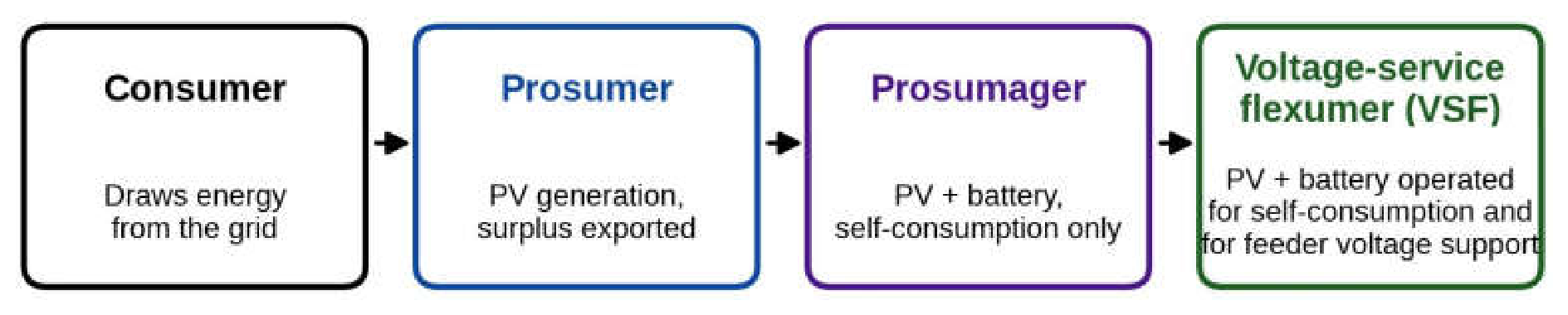
Figure 2.
Mean daily profile over the seven days: maximum pole voltage, LV busbar voltage and total prosumer export.
Figure 2.
Mean daily profile over the seven days: maximum pole voltage, LV busbar voltage and total prosumer export.
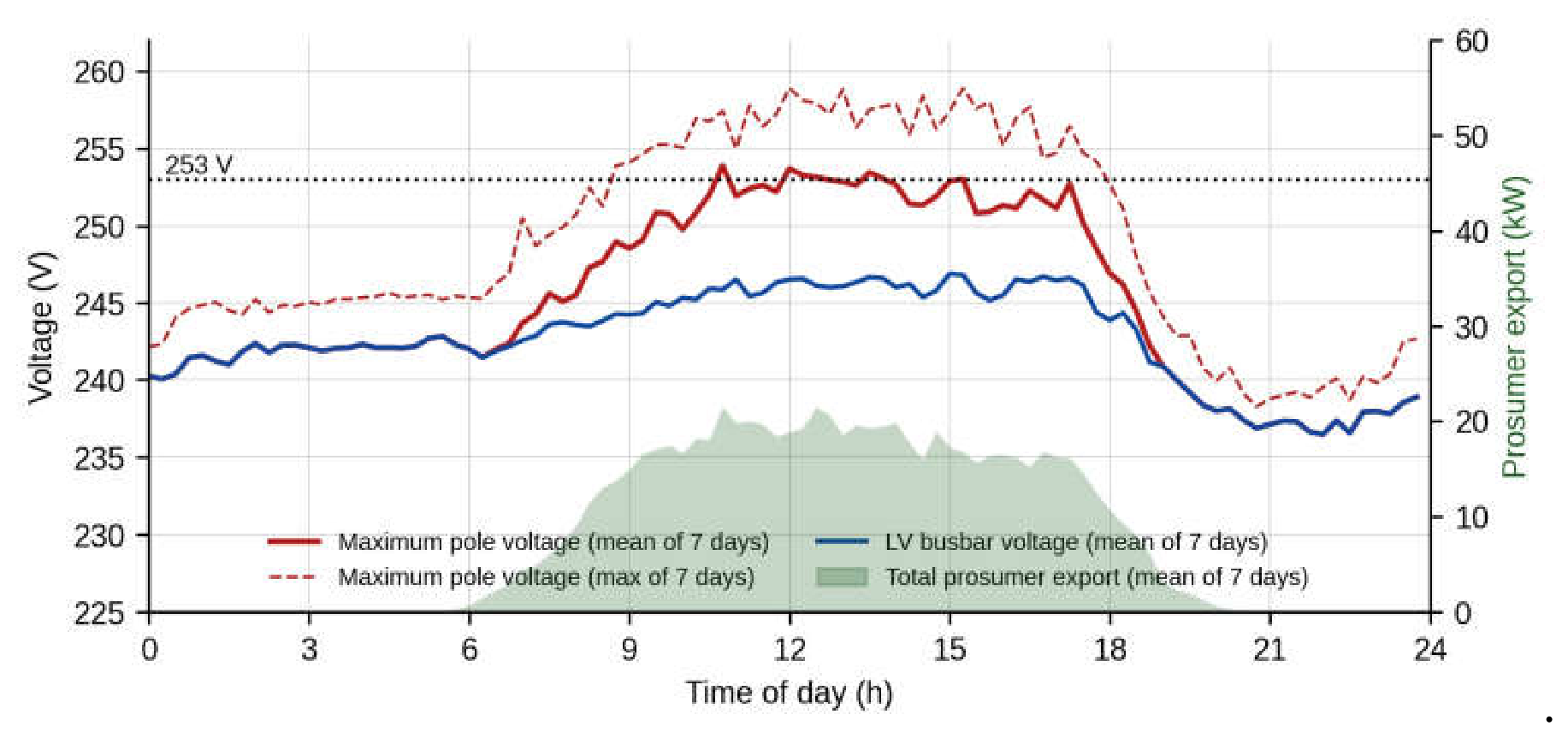
Figure 3.
Workflow of the proposed approach and split of the seven days into training, calibration and test sets.
Figure 3.
Workflow of the proposed approach and split of the seven days into training, calibration and test sets.

Figure 4.
Leave-one-day-out cross-validation error of ridge regression as a function of the regularisation parameter; the selected value is marked.
Figure 4.
Leave-one-day-out cross-validation error of ridge regression as a function of the regularisation parameter; the selected value is marked.
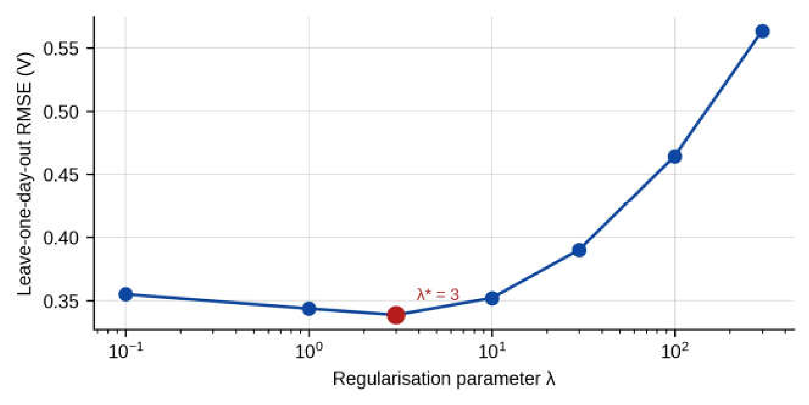
Figure 5.
Root-mean-square error of the predicted voltage rise for five estimators on the calibration day, on the test days and on the test days for voltages above 250 V.
Figure 5.
Root-mean-square error of the predicted voltage rise for five estimators on the calibration day, on the test days and on the test days for voltages above 250 V.
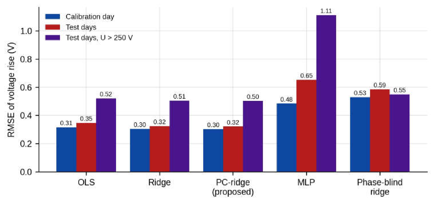
Figure 6.
Distribution of the 5808 own-phase active-power coefficients for unconstrained ridge and for PC-ridge (logarithmic scale; values clipped to the interval from −0.5 to 0.3 V/kW).
Figure 6.
Distribution of the 5808 own-phase active-power coefficients for unconstrained ridge and for PC-ridge (logarithmic scale; values clipped to the interval from −0.5 to 0.3 V/kW).
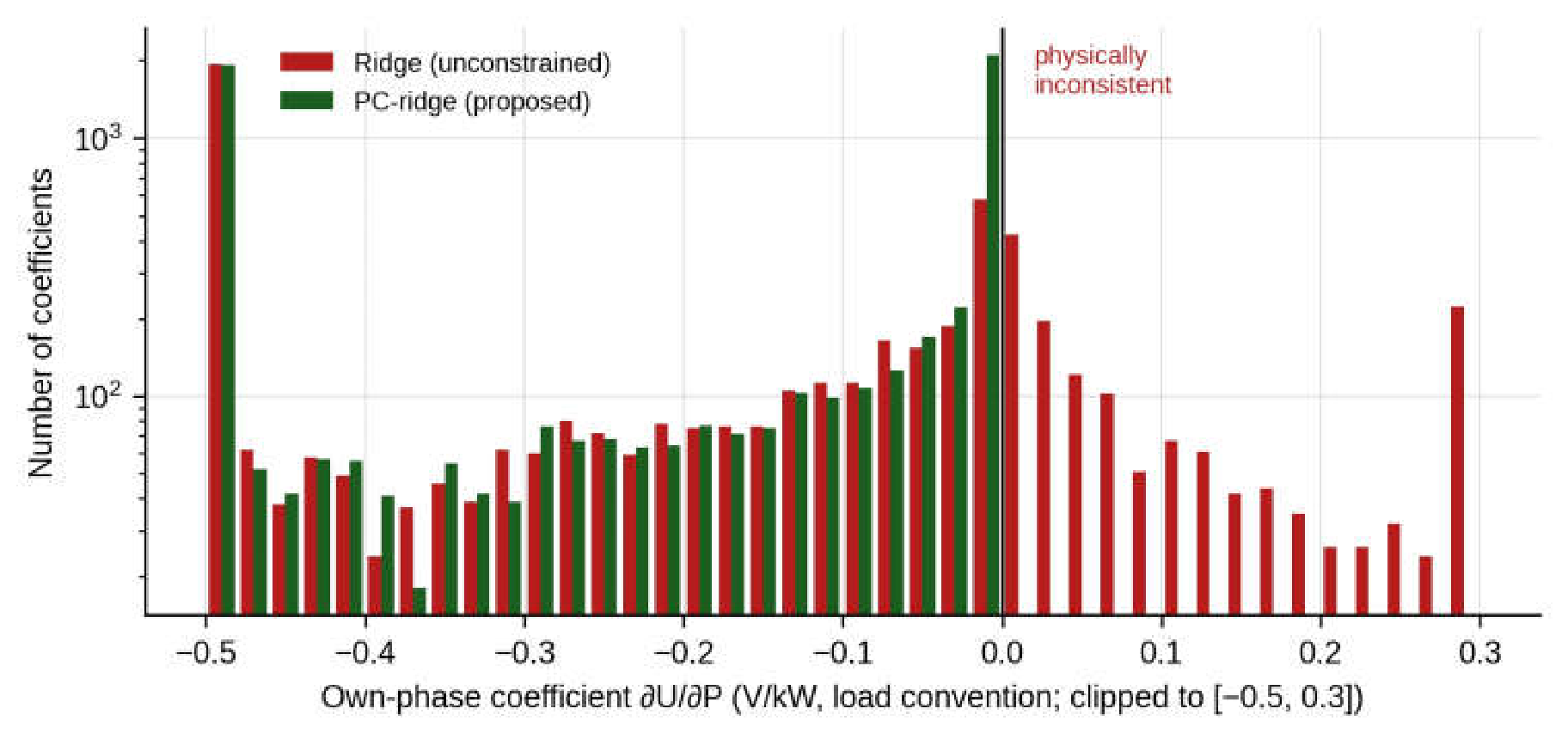
Figure 7.
Learned own-phase voltage rise per kilowatt injected, for each prosumer channel, against the section index of its pole along the feeder.
Figure 7.
Learned own-phase voltage rise per kilowatt injected, for each prosumer channel, against the section index of its pole along the feeder.
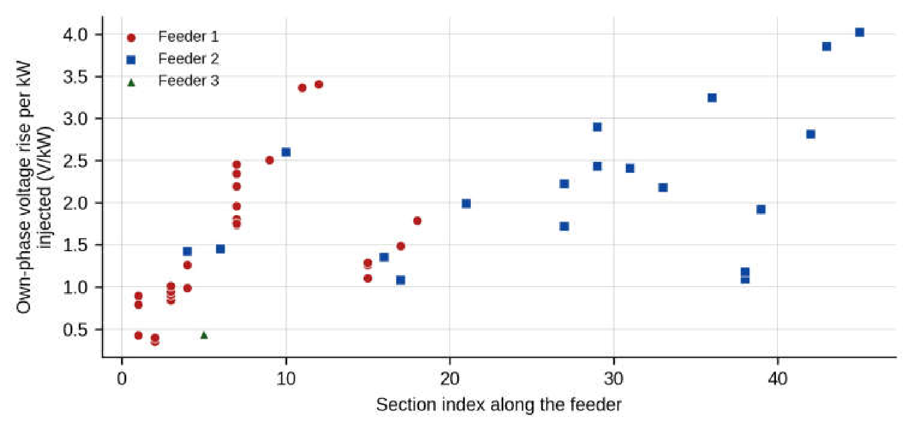
Figure 8.
Distribution of the 385 calibration scores, defined as the maximum under-prediction of the incremental model over the monitored node-phases; the 95% margin is marked.
Figure 8.
Distribution of the 385 calibration scores, defined as the maximum under-prediction of the incremental model over the monitored node-phases; the 95% margin is marked.
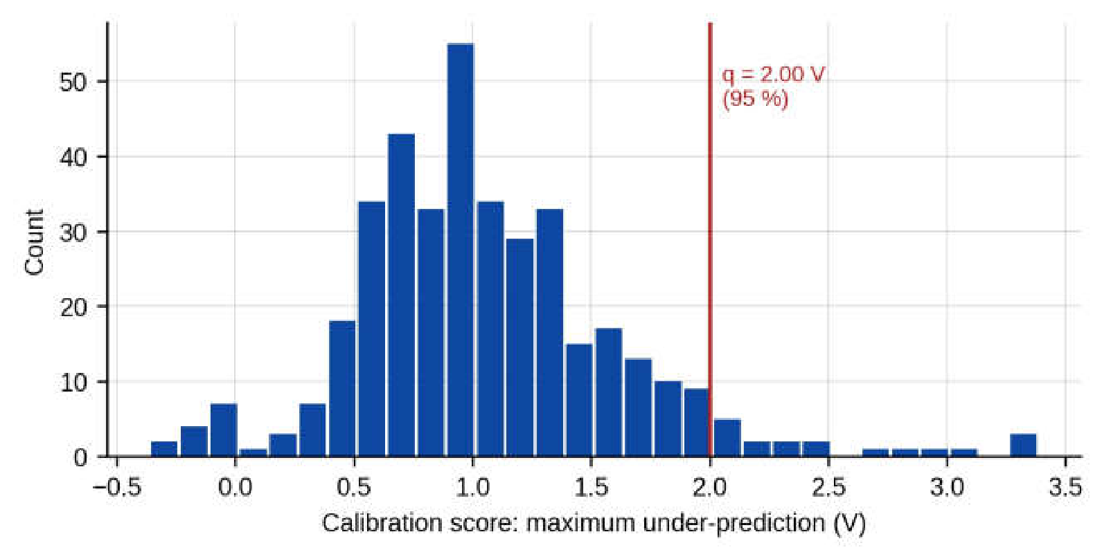
Figure 9.
Nominal versus empirical out-of-sample coverage of the conformal margin; the labels give the margin at each level.
Figure 9.
Nominal versus empirical out-of-sample coverage of the conformal margin; the labels give the margin at each level.
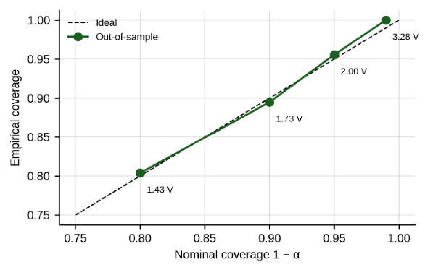
Figure 10.
Number of batteries charging in each solution of the absorption LP, for three variants of the controller.
Figure 10.
Number of batteries charging in each solution of the absorption LP, for three variants of the controller.
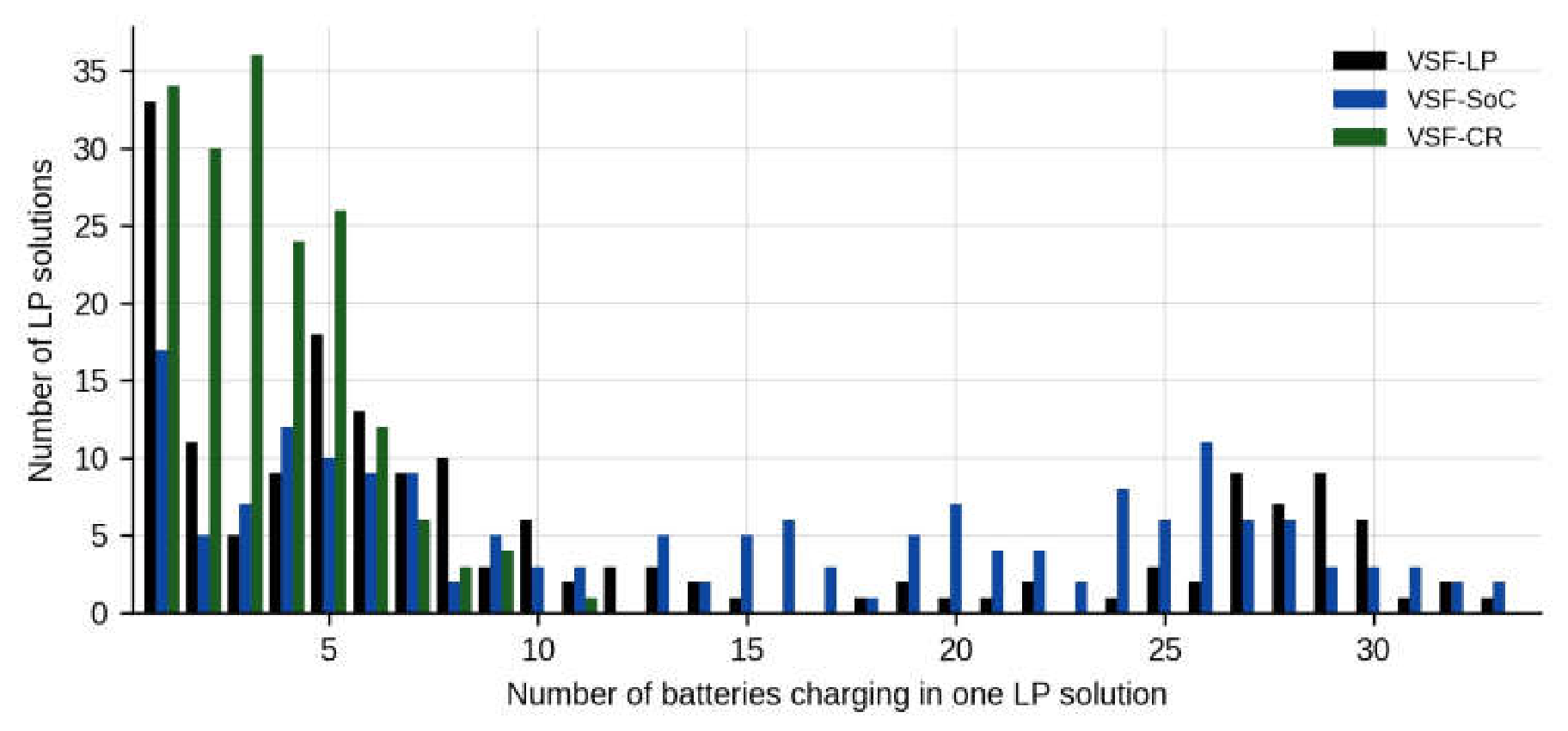
Figure 11.
Largest voltage shadow price of each solution of the absorption LP for VSF-CR over the seven days.
Figure 11.
Largest voltage shadow price of each solution of the absorption LP for VSF-CR over the seven days.
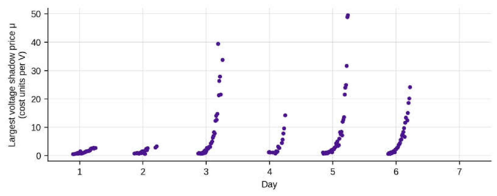
Figure 12.
Export-headroom reserve as a function of the time of day: mean and 90th percentile over the batteries.
Figure 12.
Export-headroom reserve as a function of the time of day: mean and 90th percentile over the batteries.
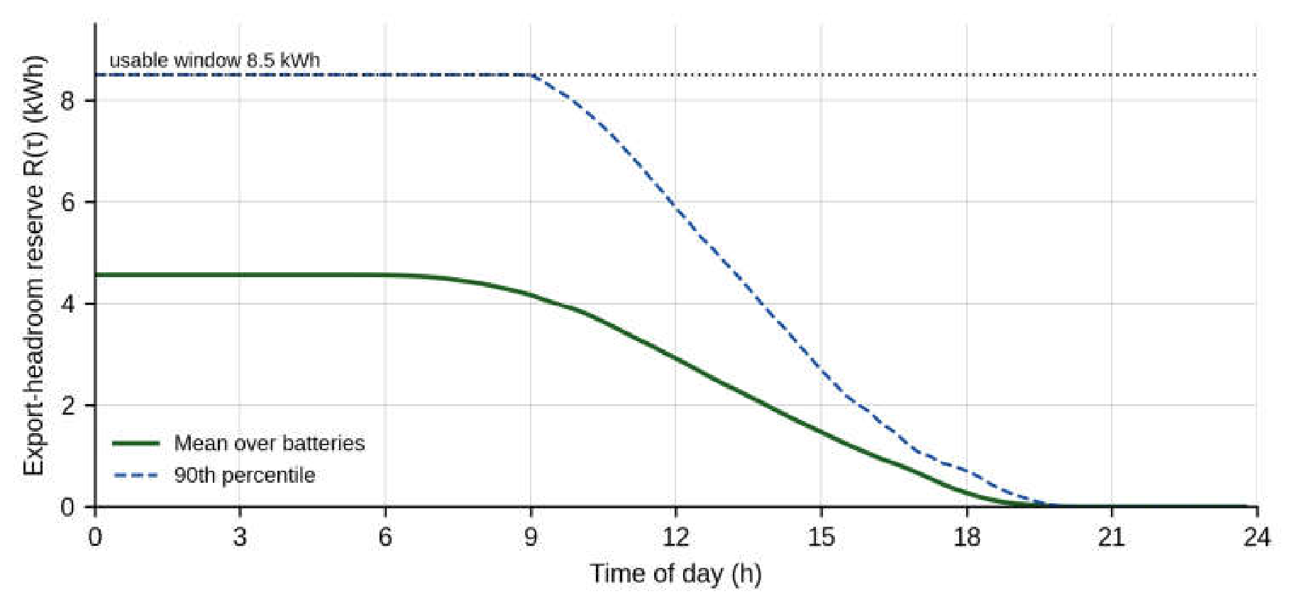
Figure 13.
Distribution of the discharge scaling factor in the 64 intervals in which it was active.
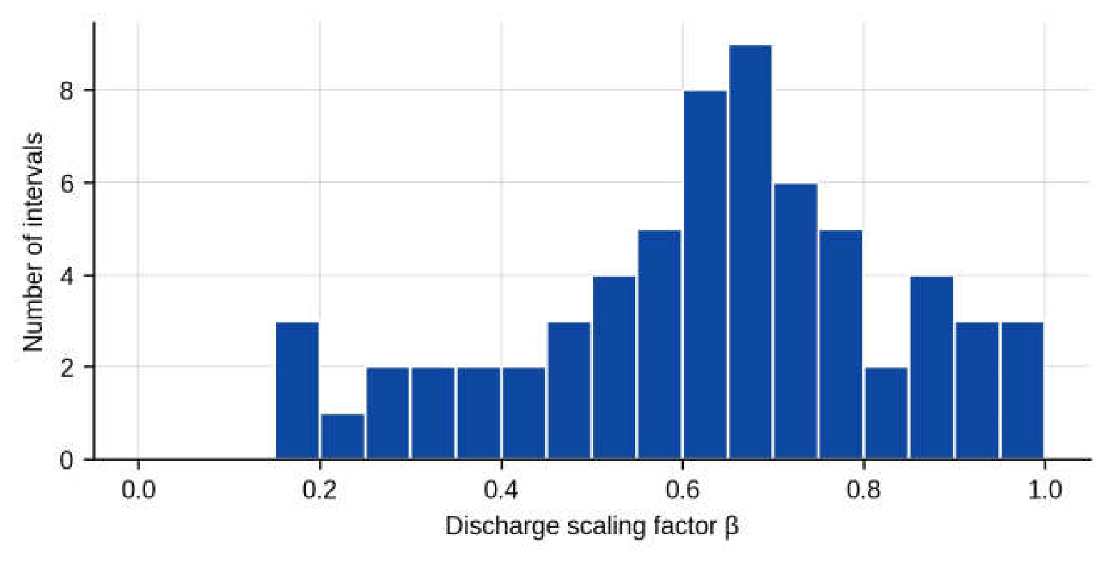
Figure 14.
Maximum pole voltage over the week for four strategies; the shaded area marks the test days.
Figure 14.
Maximum pole voltage over the week for four strategies; the shaded area marks the test days.
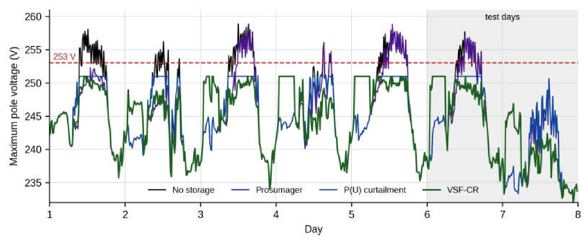
Figure 15.
Number of 15-min intervals with at least one voltage above 253 V for all strategies.
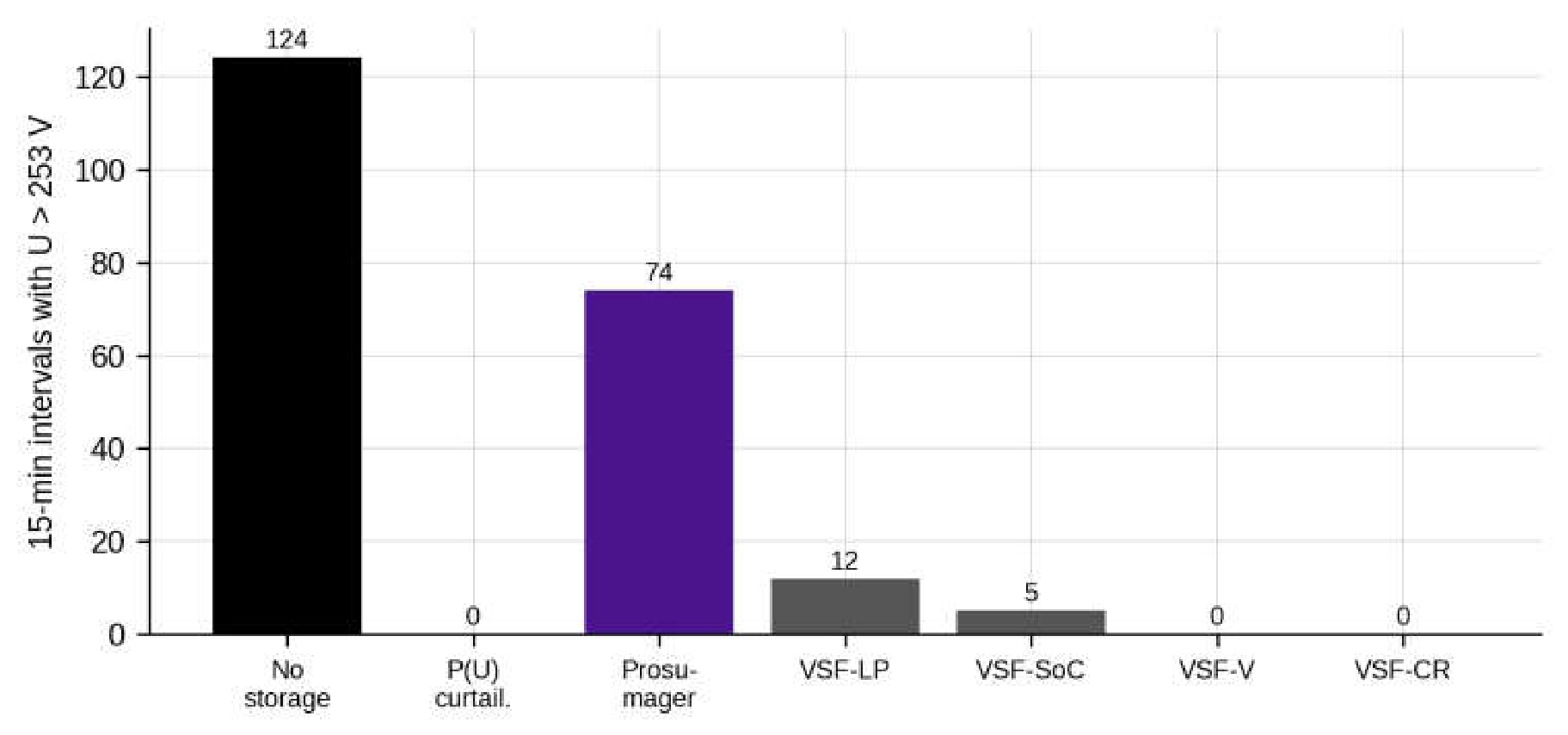
Figure 16.
Energy curtailed, energy delivered by the batteries to the owners’ demand and energy absorbed from the network over the week.
Figure 16.
Energy curtailed, energy delivered by the batteries to the owners’ demand and energy absorbed from the network over the week.
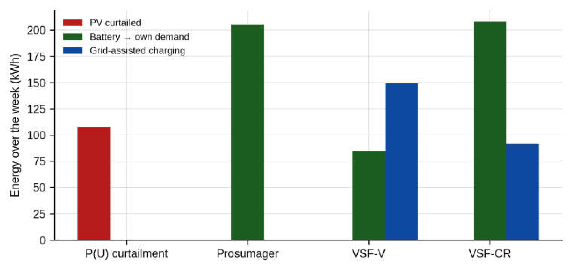
Figure 17.
State of charge of the batteries over the week for the prosumager, VSF-V and VSF-CR.
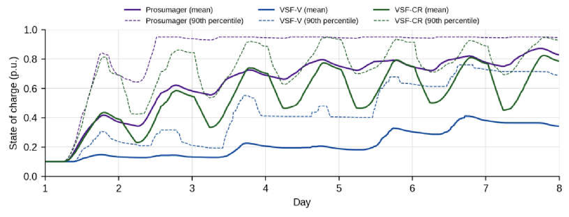
Figure 18.
Distribution of the pole voltages of feeder 1 between 10:00 and 17:00 on each phase.
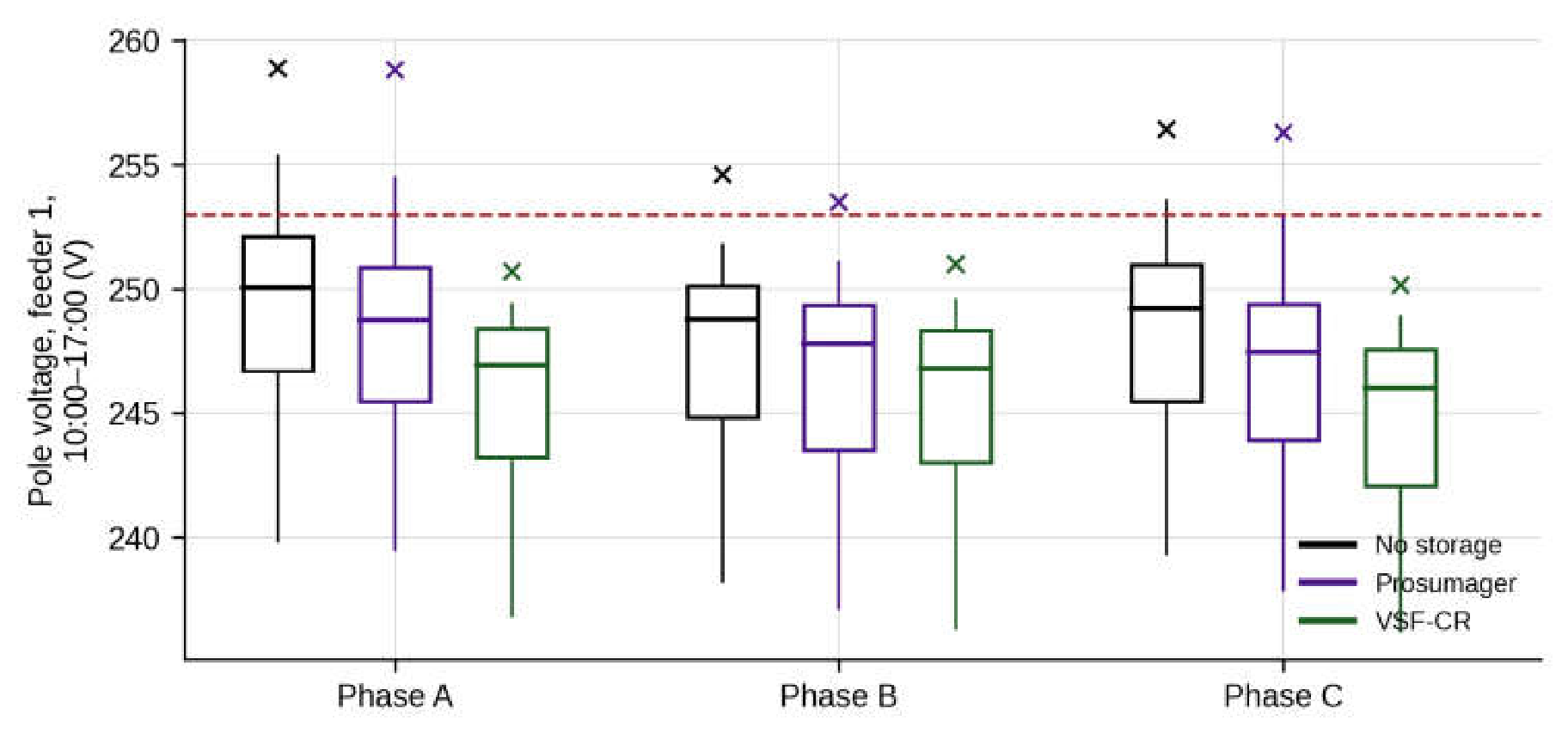
Figure 19.
Effect of the reserve coefficient on the number of intervals with voltage above 253 V (bars) and on the energy delivered to the owners’ demand (line).
Figure 19.
Effect of the reserve coefficient on the number of intervals with voltage above 253 V (bars) and on the energy delivered to the owners’ demand (line).
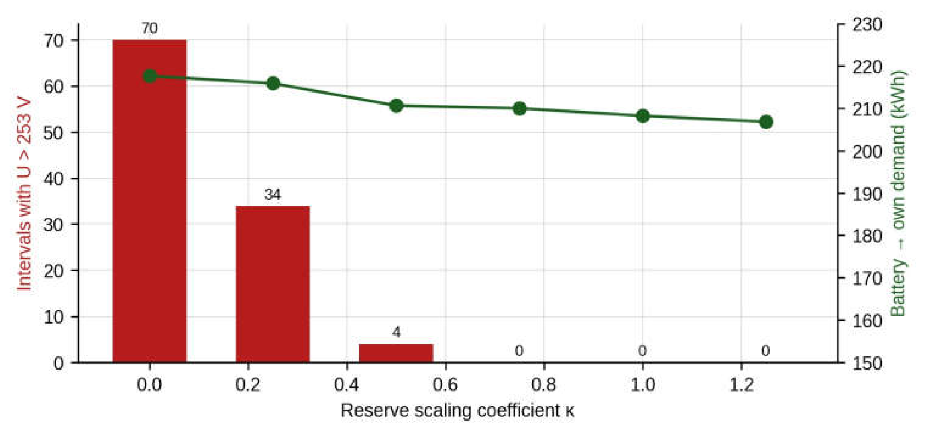
Figure 20.
Number of intervals with voltage above 253 V as a function of the battery capacity per prosumer.
Figure 20.
Number of intervals with voltage above 253 V as a function of the battery capacity per prosumer.
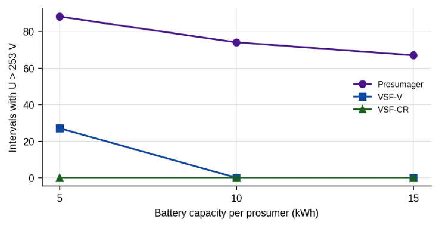
Figure 21.
Energy delivered by the batteries to the owners’ demand as a function of the battery capacity per prosumer.
Figure 21.
Energy delivered by the batteries to the owners’ demand as a function of the battery capacity per prosumer.
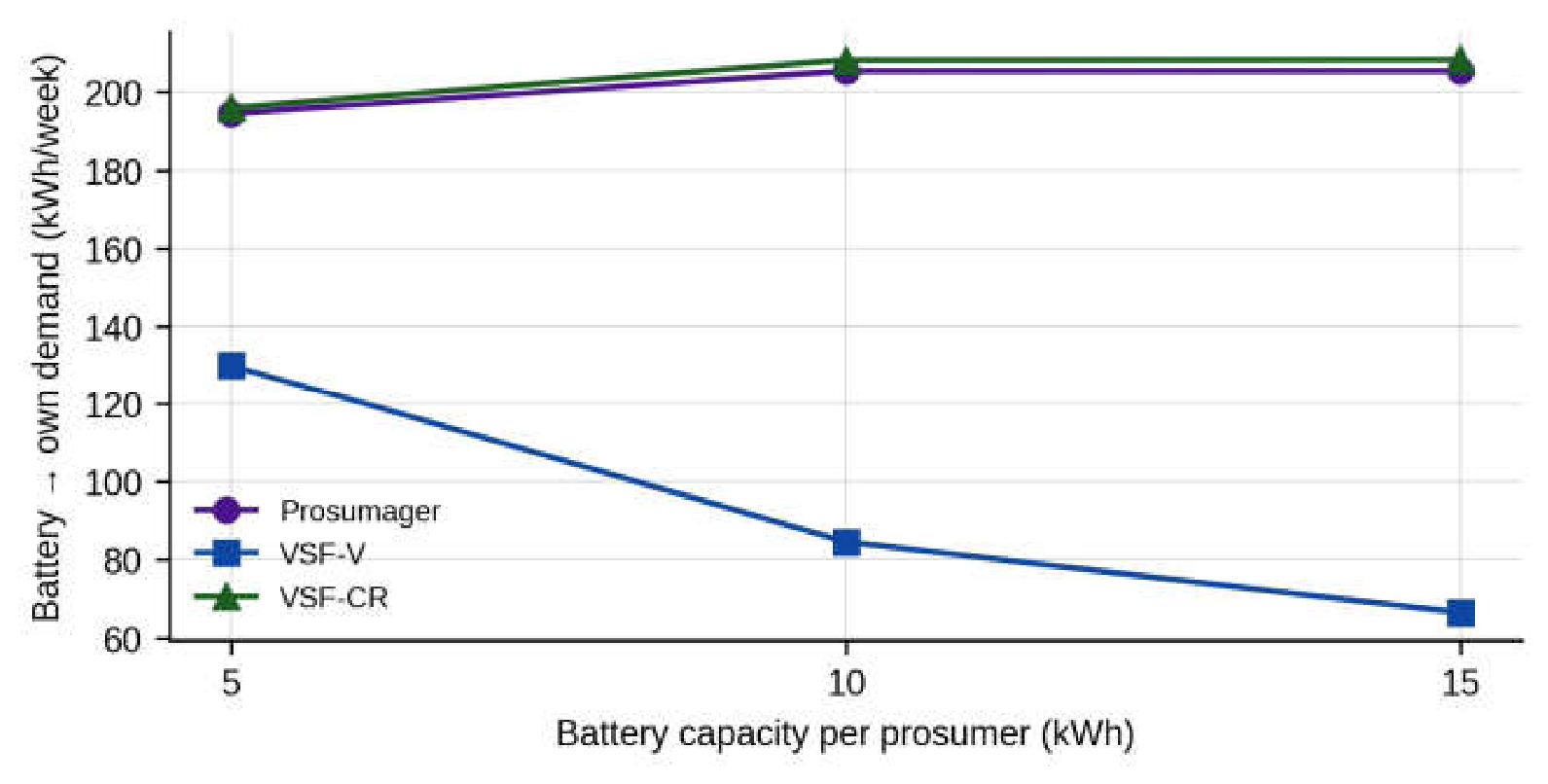
Table 1.
Positioning of the proposed approach with respect to representative related work.
| Reference | Approach | C1 | C2 | C3 | C4 | C5 | C6 | C7 | C8 |
|---|---|---|---|---|---|---|---|---|---|
| [12] | Local reactive power control of PV inverters | – | – | – | – | – | – | ✓ | – |
| [13] | Coordinated active power curtailment | – | – | – | – | – | – | – | – |
| [15] | Tap changer control without remote monitoring | ✓ | – | – | – | – | – | ✓ | – |
| [17] | Local strategies for PV-storage systems | – | – | – | – | ✓ | ◐ | ◐ | – |
| [18] | Decentralized storage charging for residential feeders | – | – | – | – | ✓ | ◐ | ✓ | – |
| [19] | Consensus-based coordination of distributed storage | – | – | – | – | ✓ | – | ✓ | – |
| [20] | Distributed battery control with SoC balancing | – | – | – | – | ✓ | – | ✓ | ◐ |
| [25] | Model-based sensitivities, unbalanced networks | ✓ | – | ✓ | – | – | – | – | – |
| [27] | Sensitivity estimation from measurements | – | ✓ | – | – | – | – | – | – |
| [28] | Measurement-based sensitivities, unbalanced networks | ✓ | ✓ | – | – | – | – | – | – |
| [32] | Deep reinforcement of learning voltage control | – | ✓ | – | – | – | – | ✓ | – |
| [38] | Conformal safety certificates for planning | – | ✓ | – | ✓ | – | – | – | – |
| [22] | Storage placement in four-wire LV networks | ✓ | – | – | – | ◐ | – | ✓ | – |
| [23] | Tap changer, Q(U) and battery control, four-wire model | ✓ | – | – | – | ✓ | – | ✓ | – |
| This paper | ✓ | ✓ | ✓ | ✓ | ✓ | ✓ | ✓ | ✓ |
Table 2.
Main characteristics of the test network and of the data set.
| Item | Value |
|---|---|
| Supply | 20/0.4 kV, 250 kVA secondary substation |
| Feeders | 4 overhead feeders, spans of approx. 40 m |
| Nodes with voltage data | LV busbar + 121 pole nodes, 3 phases each |
| Users | 231 (173 consumers, 58 prosumers) |
| Prosumer connection | 54 single-phase (A: 14, B: 22, C: 18), 4 three-phase |
| Prosumer inverters | 52 × 10 kVA, 3 × 16 kVA, 2 × 6 kVA, 1 × 5 kVA |
| Prosumers exporting in the period | 44 |
| Period | 7 consecutive summer days, 15-min resolution (672 intervals) |
| Energy consumed / exported | 1744 kWh / 1329 kWh |
| Busbar voltage (min / mean / max) | 231.9 / 242.7 / 251.0 V |
| Maximum pole voltage | 258.9 V |
| Intervals with at least one voltage above 253 V | 124 of 672 |
Table 3.
Main notation.
| Symbol | Meaning |
|---|---|
| ) | |
| Voltage rise of the node-phases above the busbar voltage of the same phase | |
| ) | |
| Set of own-phase active-power coefficients subject to sign restriction | |
| Discharge scaling factor |
Table 5.
Strategies compared.
| Strategy | Battery operation | Learned sensitivities | Network absorption | Reserve and safe discharge |
|---|---|---|---|---|
| No storage | – | – | – | – |
| P(U) curtailment | – (PV curtailed instead) | ✓ | – | – |
| Prosumager | Rule (13) | – | – | – |
| VSF-LP | ✓ | – | – | |
| VSF-SoC | LP (14)–(17) | ✓ | – | – |
| VSF-V | LP (14)–(17) | ✓ | ✓ | safe discharge only |
| VSF-CR (proposed) | LP (14)–(17) + LP (20)–(21) | ✓ | ✓ | ✓ |
Table 6.
Parameters of the case study.
| Parameter | Value |
|---|---|
| 253 V (230 V + 10%, [50]) | |
| 0.95 | |
| Battery energy / power | 10 kWh / 5 kW (5 kWh/2.5 kW and 15 kWh/5 kW) |
| Usable SoC window | 0.10–0.95 of nominal energy |
| Charging / discharging efficiency | 0.95 / 0.95 |
| Initial SoC | 0.10 |
| 1.0 | |
| Monitoring band for constraints (15) | |
| Conformal pair horizon / window / threshold | 2 h / 06:00–20:00 / 248 V |
| Evening discharge window / night reset | 17:00–07:00 / 01:00–06:00 |
| 30 | |
| LP solver | HiGHS dual simplex [51] |
Table 7.
Accuracy of the voltage-rise estimators (V).
| Model | RMSE train | RMSE calibration | RMSE test |
Max. abs. error test |
RMSE test, U > 250 V |
|---|---|---|---|---|---|
| OLS | 0.156 | 0.314 | 0.346 | 3.12 | 0.521 |
| Ridge | 0.159 | 0.304 | 0.323 | 2.80 | 0.505 |
| PC-ridge (proposed) | 0.162 | 0.302 | 0.321 | 2.81 | 0.503 |
| MLP (64 hidden units) | 0.271 | 0.483 | 0.652 | 5.39 | 1.111 |
| Phase-blind ridge | 0.318 | 0.529 | 0.586 | 4.53 | 0.549 |
Table 8.
Effect of the conformal margin on the VSF-CR controller (one week).
| Nominal level | (V) | Intervals > 253 V | (V) | Intervals above operating limit | Absorption from network (kWh) | Battery → own demand (kWh) |
|---|---|---|---|---|---|---|
| – | 0.00 | 1 | 253.1 | 1 | 42.1 | 207.1 |
| 0.80 | 1.43 | 0 | 251.6 | 0 | 73.7 | 208.4 |
| 0.90 | 1.73 | 0 | 251.3 | 0 | 82.3 | 208.3 |
| 0.95 | 2.00 | 0 | 251.0 | 0 | 87.1 | 208.2 |
| 0.99 | 3.28 | 0 | 251.3 | 29 | 365.6 | 217.3 |
Table 9.
Controller diagnostics over the week.
| Variant | LP solutions | Saturated solutions | Mean / max batteries charging | Batteries used | Share of top-5 batteries | Voltage-service energy (kWh) |
|---|---|---|---|---|---|---|
| VSF-LP | 176 | 42 | 11.0 / 33 | 39 | 41% | 196.2 |
| VSF-SoC | 176 | 13 | 14.4 / 33 | 38 | 35% | 223.6 |
| VSF-CR | 176 | 0 | 3.5 / 11 | 24 | 65% | 146.3 |
Table 10.
Results over the week with 10 kWh/5 kW batteries (the last column for test days 6–7).
| Strategy | (V) | Intervals > 253 V | Node-phase-interv. > 253 V | VVI (V·h) | Curtailed (kWh) | Battery → own demand (kWh) | Absorption from network (kWh) | Test interv. > 253 V |
|---|---|---|---|---|---|---|---|---|
| No storage | 258.9 | 124 | 2622 | 925.3 | 0 | 0 | 0 | 23 |
| P(U) curtailment | 251.0 | 0 | 0 | 0 | 107.5 | 0 | 0 | 0 |
| Prosumager | 258.8 | 74 | 1506 | 531.3 | 0 | 205.4 | 0 | 21 |
| VSF-LP | 255.7 | 12 | 125 | 31.0 | 0 | 89.5 | 0 | 6 |
| VSF-SoC | 254.5 | 5 | 41 | 8.5 | 0 | 99.9 | 0 | 5 |
| VSF-V | 251.2 | 0 | 0 | 0 | 0 | 84.6 | 149.5 | 0 |
| VSF-CR (proposed) | 251.0 | 0 | 0 | 0 | 0 | 208.3 | 91.2 | 0 |
Disclaimer/Publisher’s Note: The statements, opinions and data contained in all publications are solely those of the individual author(s) and contributor(s) and not of MDPI and/or the editor(s). MDPI and/or the editor(s) disclaim responsibility for any injury to people or property resulting from any ideas, methods, instructions or products referred to in the content. |
© 2026 by the authors. Licensee MDPI, Basel, Switzerland. This article is an open access article distributed under the terms and conditions of the Creative Commons Attribution (CC BY) license (http://creativecommons.org/licenses/by/4.0/).
Copyright: This open access article is published under a Creative Commons CC BY 4.0 license, which permit the free download, distribution, and reuse, provided that the author and preprint are cited in any reuse.