

Submitted:
13 November 2026
Posted:
17 November 2026
You are already at the latest version
Abstract
Environmental thermodynamics provides a common framework for many
of the complex problems arising from growing environmental pressures and the
challenges of sustainable development, allowing to formulate them in terms of energetic
constraints. We discuss this perspective with three
examples spanning scales from soil pores to the planet. First, we illustrate how microbial
cooperation in soils can shift the feasibility boundaries of organic-matter
oxidation, allowing syntrophic reactions that would otherwise be energetically
inaccessible. Second, we map the hydrologic cycle onto a Rankine engine
whose finite-time operation is scheduled by a self-excited land--atmosphere
oscillator, linking thermodynamic work, hydrologic storage, and rainfall
intermittency. Finally, we present the thermodynamic basis of climate change
and how modern large-scale computation couples to climate, adding to
environmental pressure. Together, these examples show how environmental
thermodynamics can provide a productive framework for interdisciplinary
research and education.
Keywords:
environmental thermodynamics
; exergy
; nonequilibrium thermodynamics
; hydrologic cycle
; finite-time thermodynamics
; syntrophy
; climate change
; computation
; maximum entropy production
1. Introduction
The complexity of environmental problems requires crossing disciplinary boundaries and seeking principles underlying different processes. Energy and its transformations often provide such a common currency for describing and predicting how environmental systems function. Water changes phase as it moves through soils, plants, and the atmosphere. Radiation drives climate and photosynthesis and powers photovoltaic technologies. Chemical free energy governs rock weathering, wildfire combustion, microbial metabolism, and the transformations that sustain biogeochemical cycles. At the same time, the built environment increasingly couples flows of heat, mass, energy, and information directly to these natural reservoirs.
This connection has become especially important for sustainable energy and for the mitigation of and adaptation to climate change. Sustainable technologies cannot be understood independently of the environmental processes and reservoirs with which they interact. Conversely, many environmental questions are sharpened by concepts first developed for engineered systems, including efficiency, availability (exergy), irreversibility, and optimization under constraints [1,2,3]. Environmental thermodynamics therefore offers a natural bridge between environmental science and technology, and more broadly among disciplines that often describe closely related energetic processes in different languages.
Beyond extremum principles, whose applicability has been only case specific [4,5,6], thermodynamic reasoning is especially valuable in complex, multiscale environmental systems as it helps identify conserved quantities, admissible transformations, generalized forces and fluxes, and limits on conversion, providing a physical filter for models that would otherwise be underconstrained.
This paper develops this perspective through three examples that span scales from soil pores to the planet and move between natural and engineered systems that increasingly share the same environmental reservoirs. Section 2 introduces the common thermodynamic tools for open environmental systems. We then consider:
- Soil redox thermodynamics and syntrophy (Section 3). Soil moisture reorganizes microbial free-energy landscapes, from water limitation during drying to redox depletion during wetting. Syntrophic butyrate oxidation becomes feasible only when a methanogenic partner lowers hydrogen below its thermodynamic threshold.
- The hydrologic cycle as a steam engine (Section 4). A Rankine-like parcel cycle is embedded in self-excited land–atmosphere dynamics, linking Lagrangian and Eulerian views and giving the finite-time power of the engine.
- Climate change and data centers (Section 5). Computation runs far above Landauer’s bound, and the emissions from its electricity can trap far more energy than data centers reject as heat. This could consume a substantial share of the remaining 1.5 °C carbon budget, while global warming raises the electricity and water demand of cooling.
2. The Common Thermodynamic Currency of Open Environmental Systems
2.1. Available Energy (Exergy)
Environmental systems can be treated as control volumes that exchange heat with reservoirs at temperatures , deliver work , and exchange mass flows with specific enthalpy and entropy [1,7,8,9]. The first and second laws read
When the surroundings act as a reservoir at temperature , pressure and chemical potentials , the maximum work obtainable as the system comes to equilibrium with them is its exergy [1,2],
Combining Equations (1) and (2) with gives the Gouy–Stodola relation for the work lost to irreversibility,
On the land surface, most of the exergy of sunlight is destroyed on absorption. Part of the remainder is lost as vapour mixes into unsaturated air, the irreversibility that limits the hydrologic engine of Section 4, and part is dissipated by microbial metabolism in the soil (Section 3). The same accounting applies to engineered systems, from a cooling tower to a data centre (Section 5).
2.2. Environmental Currencies
Three potentials carry much of the exergy in the examples below:
- Electrons. For a redox reaction with reaction quotient , the Gibbs energy iswhere n electrons are transferred across a redox potential difference and F is Faraday’s constant. A reaction is favourable when , but microbial growth requires a margin: must exceed a minimum energy quantum of order 20 kJ , needed to make ATP [10,11]. The term is the handle through which transport and biological partners alter feasibility, the theme of Section 3.
- Water. Per unit mass, the chemical potential of water relative to free liquid water at the same temperature iswith J and including matric, osmotic, and gravitational contributions [12]. The two branches meet at equilibrium through the Kelvin relation [13]. In drying soil, declining makes water increasingly costly to retain (Section 3). Above the soil, measures the work lost when vapour mixes into unsaturated air (Section 4) and the resource exploited by evaporative cooling (Section 5).
- Radiation and heat. Blackbody radiation at temperature T carries an energy flux and an entropy flux . Sunlight ( K) received near K is a high-exergy source, whose convertible fraction is given by the Petela–Landsberg expression [14,15]. Earth re-emits approximately the same energy at about 255 K with much greater entropy, and the difference corresponds to the entropy production that sustains the Earth system [16,17]. Heat itself has an exergy fraction , which sets both the cost of rejecting it and the value of recovering it, in planetary and engineered systems alike (Section 5).
2.3. Forces, Fluxes, and the Selection of Constitutive Branches
Entropy production is a sum of products of fluxes and conjugate forces [8,18],
such as heat flux and , diffusive flux and , or reaction rate and affinity . Close to equilibrium the fluxes are linear in the forces, with symmetric Onsager coefficients [19]. Environmental systems are usually far from this regime: their constitutive laws are strongly nonlinear and often admit several branches for the same forcing, among which the second law, fixing only the sign of Equation (7), cannot choose. Extremum principles such as maximum entropy production (MEP) or minimum dissipation have been widely tried [20,21], but they are not generally valid [5,6,22]. For dissipative systems without cross-coupling, a more general route builds the variational structure from the constitutive laws themselves. For a force–flux relation , the transport potential and its Legendre-dual co-content , with , make the operating state stationary at given force or given flux [23].
A common case is the exchange of stability between two constitutive branches (Figure 1), which describes the transitions from laminar to turbulent flow, from conduction to convection, and from abiotic to biotic degradation. At low throughput the realized relation is linear; at a threshold this branch loses stability and a nonlinear one takes over (Figure 1a). The exchange also changes how the dissipation is shared between the two potentials: on the linear branch, whereas on a power-law branch, , tends to . Because the potentials are proportional to the dissipation only within a power-law branch, an extremum principle fitted to one branch may fail on the other. The new branch is carried by a stock fed by the throughput, such as the kinetic energy of eddies or rolls or a microbial biomass, which acts as the order parameter A of a dynamic, nonequilibrium phase transition (Figure 1b).
Many environmental transitions are instances or variants of this picture. The channelization of landscapes resembles the onset of turbulence [24]. Rayleigh–Bénard convection, the archetypal dissipative structure [18], has the same truncated dynamics as a resource–consumer chemostat, with conduction, the kinetic energy of the rolls and the onset of convection playing the roles of abiotic degradation, consumer biomass and consumer invasion. Beyond onset, the interior temperature difference, a force, is pinned at an -like level, just as the resource is [25,26]. Methanogens invade the syntrophic consortium of Section 3 in the same transcritical way, and microbial decomposition pins soil carbon at its own [27,28]. Variants differ in the shape of the potential V, or become self-excited oscillations, as in the hydrologic engine of Section 4. In its bistable variants, the same picture underlies the tipping elements of the climate system [29,30] and the catastrophic shifts of ecosystems [31,32]: vegetation–rainfall feedbacks in drylands and monsoon regions, forest dieback, ice sheets, permafrost and the overturning circulation of the ocean. There, too, a stock (biomass, ice volume, soil carbon, ocean heat) acts as order parameter, and the structured and unstructured states are distinct dissipative branches that coexist over a range of forcing.
3. Complex Thermodynamics of Soil Reaction Networks
3.1. Ecohydrology and Thermodynamics of Organic-Matter Decomposition
Our first example concerns how soil water availability affects microbial activity, through the chemical potential of soil water (Equation (6)) and the redox potential of the complex reaction network responsible for organic-matter decomposition [12]. These reactions remain largely unexplored from a thermodynamic point of view. On the dry side, falling water potential forces cells to spend energy on osmolytes, while substrate diffusion through thinning water films slows [33,34]. On the wet side, gas-filled pores close, oxygen resupply fails, and respiration climbs a ladder of electron acceptors [35],
each step yielding less free energy per electron, from about kJ per mol with oxygen to about kJ per mol with sulfate and CO2 (Figure 2). Aerobic respiration dominates below a water-filled pore space (relative soil moisture s) of about , and methanogenesis takes over near saturation [36]. Microbes are thus squeezed between a water-energy barrier when dry and a shrinking, eventually inverted, redox yield when wet. By controlling gas exchange, moisture reorganizes the free-energy landscape available to metabolism.
3.2. Microbial Cooperation Alters Thermodynamic Feasibility in Soil Syntrophy
At the wet end of the ladder, some reactions run only in partnership [10,37,38], as in the classic coupling of butyrate oxidation and hydrogenotrophic methanogenesis,
With the other activities fixed, Equation (5) expresses both reaction energies through the dissolved hydrogen concentration H,
Here kJ is the minimum energy increment of Section 2 [10]. , set by the butyrate and acetate concentrations, is the level at which the oxidizer conserves exactly this increment. , set by the CH4 and CO2 partial pressures, is the level at which methanogenesis yields no energy. Requiring both partners to conserve at least gives the window
which is 16–240 nM for M butyrate, M acetate, and atm (Figure 3a). Since hydrogen is an intermediate, it cancels from the overall reaction. Per mole of butyrate (two H2, half a CH4),
independent of H. Hydrogen thus does not change the free energy available to the partnership, only how it is divided between the partners.
Population dynamics then determine whether, and where, the partnership operates within this window. In a minimalist model [39], fermentation supplies hydrogen at a rate that grows with anoxia. Diffusion through gas-filled pores removes it at a rate that falls as the pores fill, and methanogens of biomass Y consume it:
Without methanogens, hydrogen relaxes to , which rises steeply with moisture (Figure 3b). Methanogens invade when exceeds their break-even level [26]. This is a transcritical bifurcation at a critical moisture . Beyond it, methanogens hold hydrogen at regardless of supply and leakage, as observed in anoxic soils and sediments [40,41,42]. Syntrophy thus requires : microbial physiology selects the hydrogen level within bounds fixed by thermodynamics. With nM, the oxidizer obtains 32 kJ per mole of butyrate and the methanogens 23 kJ per mole of CH4, just above their floor.
The chemical entropy production, with affinities , follows directly. At coexistence the methanogens take up hydrogen at the rate , with affinity per mole, so
Entropy production vanishes on the methanogen-free branch and grows linearly from (Figure 3c), as an order parameter of the bifurcation, in the spirit of the dynamic phase transitions of Section 2.3. If the hydrogen comes from butyrate oxidation, the pair dissipates , about 10 mW of pore water in wet soil. Under intermittent rainfall, dissipation comes in pulses that lag wetting [39]. Rainfall intermittency, which climate change is increasing (Section 5), thus controls when, and how fast, soil reaction networks run.
4. The Hydrologic Cycle as a Self-Excited Engine
Driven by sunlight, the hydrologic cycle of evaporation, ascent, condensation and rain (Figure 4) works as a steam engine with water as its working fluid. Konings et al. [43] idealized it as an abbreviated Rankine cycle, extending the heat-engine theories of moist convection and tropical cyclones [44,45]. Liquid water evaporates at the surface temperature , rises and cools, condenses at colder temperatures, and returns as rain. Unlike an idealized engine, this one cannot run at any chosen rate. Its throughput, the rain that sustains ecosystems and societies worldwide, is set by the slow filling and emptying of soil and atmospheric water, making the cycle a natural example of finite-time thermodynamics.
4.1. Reservoirs and Self-Excitation
Let be the relative soil moisture of a root zone of capacity M, and the column water vapour over a land region. Their water balances are [46]
with large-scale exchange , evapotranspiration E, leakage K and infiltrating fraction f. Considering average conditions, rainfall can be assumed to follow a convective pick-up law [47,48] whose efficiency depends on soil moisture [46],
The sigmoid rises with s, because moister surfaces raise the convective available potential energy. The sigmoid falls with s, because drier surfaces help the boundary layer reach the lifting condensation level [49]. Rainfall efficiency therefore tends to peak at intermediate soil moisture. Evapotranspiration and infiltration only move water between the two reservoirs, so the system has the activator–recovery structure of the FitzHugh–Nagumo model. Soil moisture is the activator: on the CAPE side, wetting raises rainfall efficiency, which wets the soil further. Total water is the slow recovery variable, resupplied by large-scale import [46]. Self-excitation requires that wetting raise rainfall into the root zone faster than it depletes the column and accelerates evapotranspiration and drainage. This favours shallow root zones, a steep CAPE response and slow resupply.
We use the reference parameters of Ref. [46]. These include a root zone of mm, a resupply time d, a pick-up threshold mm, and evapotranspiration saturating at 5 mm above . With these values the single equilibrium is unstable and is surrounded by a limit cycle of period 72 d (Figure 5a,b). Each period has three phases:
- a convective burst of about 3 d, in which rainfall peaks at 20 mm , the column collapses to 40 mm and soil moisture jumps to ;
- a dry-down of about 50 d, in which soil moisture falls to , the column recharges to 70 mm and rainfall stays below evapotranspiration;
- a trigger, when light rain on a nearly full column returns the soil to the steep side of .
Oscillations exist for large-scale supply mm , between two Hopf bifurcations.
4.2. Parcel Thermodynamics
The limit cycle is a cycle of the reservoirs, not of the working fluid, and its area is not work. Work is done by the water itself, through a thermodynamic cycle that each kilogram completes within hours, fast compared with the evolution of s and Q. The cycle starts from the surface state at evaporation: the temperature , which falls by 1 K per rise in soil moisture around 300 K, and the relative humidity h, taken equal to the column saturation fraction ( mm) of the pick-up law [47]. The water evaporates at , mixes into the surface air, rises dry-adiabatically to the lifting condensation level and then along the pseudo-adiabat until its vapour has condensed, and returns as rain (Figure 5c). Water is the working fluid, and the dry air is part of the environment with which it exchanges heat. Condensation spreads over a range of temperatures, which can be represented by a single temperature at height . Along the orbit, ranges from about 266 K for water evaporated into the dry air after a burst (B, C in Figure 5a,b) to 275 K late in the dry-down (F, G).
The reversible work is the net heat exchanged over the cycle, [43]. The mixing step 2→3, however, is irreversible diffusion of vapour into subsaturated air [50], the water term of Equation (6): it generates entropy and delivers no work, so the attainable work is
Even w is an upper bound: re-evaporation of rain and cloud mixing add further irreversibilities, and the work is further dissipated by friction in winds and turbulence [50].
Humidity changes the shape of the cycle but hardly its work. At K, falls from 314 to 194 kJ as h rises from to , while w stays at 187 kJ to within . Drier air costs more mixing work, per unit , but also forces the water to rise higher before saturating. By Clausius–Clapeyron, condensation shifts like the dew point, , and the colder condensation adds about of Carnot work, offsetting the loss to leading order. Humidity thus decides how the cycle divides between mixing and colder condensation, not how much work a unit of water delivers, which is set by the surface temperature and the depth of condensation. About a quarter of w, kJ , lifts the condensate and is dissipated by drag as rain falls [50]; only about kJ is lost on impact.
In an endoreversible engine, a faster heat flow requires a larger temperature drop, which lowers efficiency, so power peaks at an intermediate rate [3,51,52]. In the hydrologic engine the corresponding drop is the subsaturation that drives evaporation, and since w hardly depends on h, drier air speeds up evaporation at almost no cost in work per kilogram. The usual trade-off of finite-time engines thus disappears, and power is limited instead by the surface energy supply and by how fast the reservoirs deliver water to the cycle.
The rain falling at a given time evaporated over the previous weeks or was imported. In a well-mixed column, all water leaves at the same rate whatever its age [53]. For the reference parameters, about of the column water is recycled [54], and column and root-zone water are on average 11 and 9 d old, so a local loop takes about three weeks and spans several phases of the oscillation. Because w hardly depends on h, however, following this water changes the work it carries by less than , and the engine power is simply the rain rate times the work per kilogram,
Power is strongly pulsed (Figure 5d), peaking at 44 W during the burst and decaying to about 4 W in the dry-down. Its cycle mean, W , compares with W for the reversible cycle and a latent heat throughput of 95 W . Self-excitation costs power: at the unstable steady state the engine would deliver W , about more, because the orbit spends most of its time drying down (mean soil moisture instead of ), and the concavity of adds a further penalty by Jensen’s inequality. As with the chemostat of Section 2.3 and the syntrophic pair of Section 3, the realized state is selected by a stability threshold and carried by stocks, here soil and column water.
5. From the Warming Planet to Large-Scale Computation
5.1. A Thermodynamic Primer on Climate Change
The Earth absorbs about W of sunlight [55] and rejects nearly as much in the infrared. Most of its heat capacity is in the ocean, whose upper layer exchanges heat with the atmosphere within years and whose deep layer does so over centuries. Per unit area, a minimalist model for the first law for these two reservoirs reads
where T and are the global-mean surface and deep-ocean temperatures, and their heat capacities, the coefficient of heat exchange between them [56,57], and the Stefan–Boltzmann constant. The effective emissivity , which depends on the atmospheric composition c, measures how much less the planet emits than a blackbody at its surface temperature. Equivalently, it defines the emission temperature K, that of a blackbody emitting the same flux. Since infrared radiation escapes to space mostly from the cold mid-troposphere, is roughly the temperature there. Greenhouse gases lower by raising the altitude from which infrared radiation escapes to space, where the air is colder, so the planet emits less energy [58,59]. The radiative forcing is the imbalance a change in composition would create if the temperature stayed at its pre-industrial value ,
Today’s W corresponds to a change in of only about one percent (Figure 6a). Until about 1960, warming gases and cooling aerosols grew together and nearly cancelled. The net forcing then accelerated, to about W per decade today, as emissions surged, halocarbons appeared and clean-air policies weakened aerosol cooling.
With and W yr , W , and emission rising by W per kelvin of warming, the model reproduces the observed warming since 1850 to within K (rms), with relaxation times of about three and 170 years (Figure 6b). The deep ocean, still absorbing heat, keeps the planet out of balance by W , double the value of two decades ago [60]. A single reservoir fits the record almost as well [61], but it mistakes ocean heat uptake for radiative damping, roughly halving the climate sensitivity and missing the long-term memory that sets the future. In the two-box model, holding today’s concentrations fixed adds another K by 2100; holding today’s emission rate brings CO2 near 560 ppm and warming to about K; stopping emissions nearly stops warming, because falling CO2 forcing offsets the slow warming of the deep ocean [62]. Warming also reshapes the water cycle. Atmospheric moisture, and with it heavy rainfall, rises by about per kelvin, following the Clausius–Clapeyron relation, whereas mean rainfall, limited by the atmosphere’s ability to radiate away latent heat, rises by only 1– per kelvin. Rain therefore falls in fewer but heavier events [63,64,65].
The entropy budget tells a complementary story. With the blackbody fluxes of Section 2, sunlight from the photosphere ( K) brings in entropy at the rate W ,1 while the infrared, emitted at , carries away W , twenty times more. Including the entropy stored in the reservoirs, the internal production is
This budget sees only boundary fluxes: it gives the total, not how it is shared among internal processes. Almost all of it comes from the thermalization of sunlight. The rest is material production by irreversible flows of air, water and life, each estimated from its internal flux; a heat flux from to , for instance, contributes . The hydrological cycle contributes about 30–50 mW , the dissipation of winds about 8, the biosphere about 1, and ocean currents a few hundredths [16,50,68,69,70]. This few percent drives the weather, the water cycle (Section 4) and life.
In steady state the planet emits what it absorbs, so and depends on absorbed sunlight alone. Greenhouse gases, surface temperature and circulation only move production between its radiative and material parts; the rise in evaporation of about per kelvin, for example, adds about mW to the hydrological cycle and takes the same from radiation. Warming changes the total in only two ways. While the planet is out of balance (Figure 6c), the heat N is stored at T instead of being radiated at , lowering production by mW , an effect that vanishes at equilibrium. And although is fixed in the model, retreating ice and snow raise it by about W per kelvin [71], adding a lasting mW today. All these changes are about a thousandth of the total.
Entropy production is therefore a poor indicator of climate change: doubling CO2 leaves it nearly unchanged, while temperature, rainfall and ice change substantially. For the same reason, maximizing the total production [4,68] cannot select anything, since fixes it. Possible entropy production principles can only be applied to the material part, with the radiation field as a constraint, as Paltridge did with MEP for meridional heat transport [20]; a maximum then exists because transport erodes the gradient that drives it, as in maximum power. Which subsystem to isolate, and under which constraints, remains a modelling choice that does not follow from the second law [22]. The thermodynamic signature of global warming is a redistribution of temperatures and of entropy production inside the control volume, as in the selection arguments of Section 2.3.
5.2. Impact of Data Centers in a Warming World
Data centres, increasingly driven by demand for artificial intelligence, are a fast-growing, highly concentrated use of energy that shows the difference between the heat a technology releases and the greenhouse gas it emits. In 2024 they used about 415 TWh of electricity, about of global consumption. They are projected to use about 945 TWh by 2030, just under of global consumption, and 700–1700 TWh by 2035, the upper case reaching about [72].
Thermodynamics sets only one irreducible cost on computing, that of logical irreversibility. Erasing one bit dissipates at least
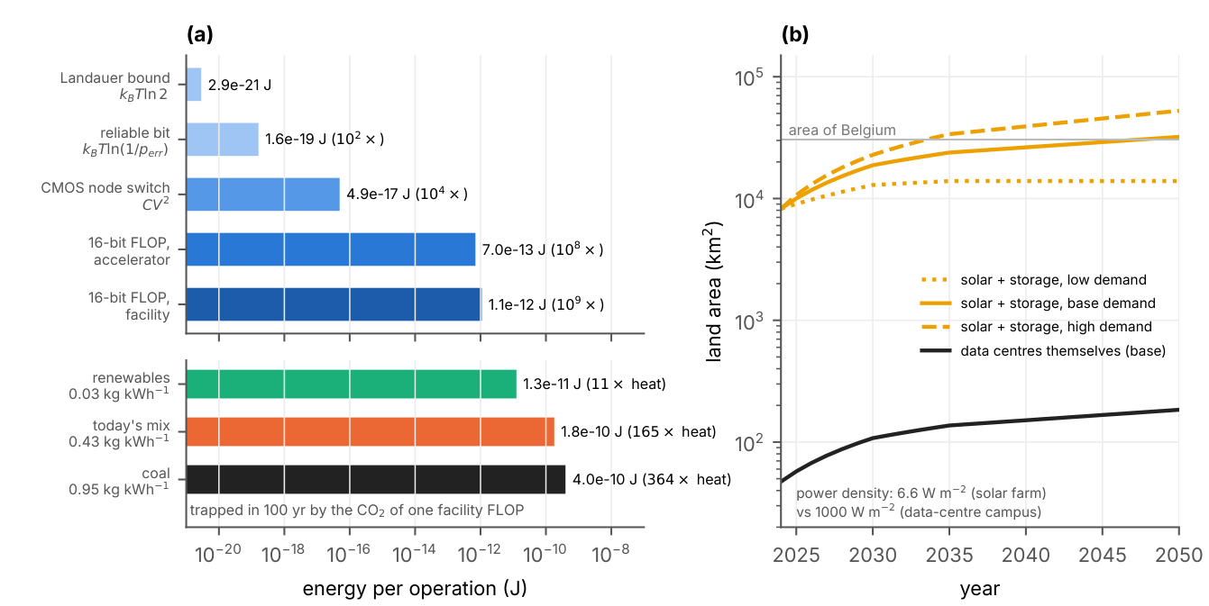
a bound proposed by Landauer [73], verified experimentally [74], and in principle avoidable by reversible computing [75,76]. Real hardware sits far above it (Figure 7a): a reliable bit needs an energy barrier 56 times larger, a CMOS switching event costs times more, and a 16-bit floating-point operation costs J on a current accelerator, or J including cooling and power delivery (power usage effectiveness [77]), about times the bound. Essentially all the electricity ends up as heat at 30–C, only slightly warmer than the environment. This heat is low-grade: less than a tenth of it could be converted back into work.
The heat must then be rejected to the environment. When the outdoor air is too warm, it must be pumped uphill against the temperature gradient, at the cost of electricity. The alternative is evaporating water, which uses the dryness of the air, the same disequilibrium that drives the hydrological cycle (Section 4) [78,79]. Warming makes both options costlier, because it raises the air temperature and the wet-bulb temperature that limits evaporative cooling. While locally the heat is intense (a 100 MW centre on 10 ha releases about 1000 W , several times the net radiation the land receives), spread over the globe, however, the heat of all data centres is only about W , more than four orders of magnitude below today’s forcing.
The climate footprint of computing therefore comes primarily from how its electricity is produced, not from its heat. In 2024 that production emitted about 180 Mt of CO2 [72]. On today’s grid, a kilowatt-hour emits about kg of CO2, which within about four months traps as much energy as the kilowatt-hour releases as heat, and within a century 160 times as much [67,80]. The factor is about 360 for coal and about 11 for renewables with storage, so the climate cost of computing exceeds its own heat by one to more than two orders of magnitude, depending on the electricity supply (Figure 7a). Extending the IEA demand cases to 2050, a sector supplied by gas or coal would emit 13–30 Gt of CO2, or 10– of the remaining 1.5 °C budget of about 130 Gt [66], against about with renewables. Renewables, however, face their own thermodynamic limit, power density. Solar farms deliver 5–10 W averaged over their land [81], two orders of magnitude less than a data centre releases. Supplying the 2050 base-case load around the clock would take some km2, the area of Belgium, against less than 200 km2 for the data centres themselves (Figure 7b).
Thermodynamics thus gives a concrete meaning to a sustainable footprint: the heat, carbon, water and land a technology demands must fit within what its surroundings can absorb, at physically attainable efficiencies. Decarbonized electricity removes the radiative cost, within the limits of renewable power density, and higher rejection temperatures reduce cooling costs and turn waste heat into a product. Every substitute brings its own boundary conditions; for ammonia, for example, N2O leaks decide whether its greenhouse footprint resembles that of renewables or exceeds that of coal [82].
6. Environmental Thermodynamics: An Exciting Agenda for Research and Education
The technosphere and the environment are increasingly coupled, often through loops in which a technology alters the conditions it depends on. Thermodynamics offers a natural frame for such problems: it bounds what natural and engineered systems can do, locates where exergy is destroyed, and provides a common language of forces, fluxes, potentials and stocks. Drawn across the boundary between a technology and its surroundings, this accounting exposes such loops and shows when an apparent efficiency gain only moves dissipation elsewhere. In open, forced systems that store energy and matter, environmental thermodynamics joins these bounds and balances with the dynamics that choose the realized state.
Environmental thermodynamics invites bold new explorations. Unlike the closed machines of classical cycle analysis, environmental engines store, pulse and exchange at multiple rates, and the reaction networks they drive join nonequilibrium chemistry, population ecology and stochastic processes, with direct bearing on greenhouse-gas emissions. Thermodynamic constraints could make reduced and machine-learning models more physical and help identify the stocks and stability criteria that select the realized states. The energy transition, too, needs accounts that cross the boundary between technology and environment, as the comparison of photosynthetic and photovoltaic conversion of the same sunlight illustrates [83].
These questions also suggest a new way of teaching thermodynamics. A conventional engineering course moves from ideal gases to pistons, Carnot cycles, steam tables and refrigeration. These remain essential, but the universality of the concepts becomes clearer when each is taught through natural and engineered systems side by side: the chemical potential of water through a reverse-osmosis membrane, a salinized soil, a transpiring leaf and a cooling tower; phase change through a heat pump and a cloud; radiation through a solar panel, a leaf and the greenhouse effect. Thermodynamics as a shared quantitative language for engineers, physicists, Earth scientists and ecologists provides a disciplined way to discuss sustainability in terms of the exergy, materials and externalities needed to maintain desirable states far from equilibrium.
This approach spans scales, from a microbial reaction to the planet, and combines equilibrium thinking (states, potentials, bounds) with nonequilibrium thinking (rates, thresholds, emergent cycles). Each example discussed here starts from simple balances and constitutive laws that sharpen deeper questions. Environmental systems are rich in organization sustained by coupled flows of energy and matter, from convection cells to river networks and microbial consortia. Building on the long search for unifying principles, from Lotka’s maximum power to maximum entropy production [4,84], this organization calls for a multidisciplinary thermodynamics that pairs, for each class of open system, the appropriate potentials with the dynamical mechanisms that select its state.
7. Conclusions
Extending thermodynamics into the environmental realm is essential for understanding and anticipating a changing world, and the environment, in turn, is a demanding and fertile frontier for thermodynamic theory. From soil pores to the planet, energy transformations and their irreversibilities let structure emerge and set the rhythms of change. Climate change itself is, in thermodynamic terms, a perturbation of the planet’s ability to reject heat, with consequences that propagate through the water cycle, the biosphere and the technosphere. Thermodynamics constrains the feasibility, direction and minimum cost of such changes; coupled with transport and kinetics, it identifies the paths accessible at finite rates and the conditions for stability and transition. Living systems add a further layer: organisms regulate their fluxes and modify their surroundings, creating feedbacks that fixed rate laws cannot capture.
Explicit accounting of energy, entropy and exergy can strengthen Earth-system and ecological models, and inform the management of soils, watersheds and cities, where optimal control offers a framework for pursuing sustainability while maintaining ecosystem services [12]. Recognizing what natural and engineered environments share also opens new opportunities for education and outreach. Environmental thermodynamics thus helps bring order to environmental complexity and guide responses to the pressing needs of nature and society.
Funding
This research received no external funding.
Data Availability Statement
No new empirical data were created. All model results and figures can be reproduced from the equations, parameters and assumptions given in the text.
Acknowledgments
This paper builds on material developed for the course Environmental Thermodynamics at Princeton University and for the presentation “Environmental Thermodynamics: Bridging Science and Technology in a Changing Environment” at the Entropy 2026 Conference in Barcelona. We thank the editors of Entropy and the conference organizers for this opportunity
Conflicts of Interest
The author declares no conflicts of interest.
Abbreviations
The following abbreviations are used in this manuscript:
| ATP | Adenosine triphosphate |
| CAPE | Convective available potential energy |
| CMOS | Complementary metal–oxide–semiconductor |
| IEA | International Energy Agency |
| LCL | Lifting condensation level |
| MEP | Maximum entropy production |
References
- Bejan, A. Advanced Engineering Thermodynamics, 4th ed.; Wiley: Hoboken, NJ, 2016. [Google Scholar]
- Szargut, J.; Morris, D.R.; Steward, F.R. Exergy Analysis of Thermal, Chemical, and Metallurgical Processes; Hemisphere: New York, 1988. [Google Scholar]
- Andresen, B.; Salamon, P.; Berry, R.S. Thermodynamics in finite time. Phys. Today 1984, 37, 62–70. [Google Scholar] [CrossRef]
- Ozawa, H.; Ohmura, A.; Lorenz, R.D.; Pujol, T. The second law of thermodynamics and the global climate system: A review of the maximum entropy production principle. Rev. Geophys. 2003, 41, 1018. [Google Scholar] [CrossRef]
- Martyushev, L.M.; Seleznev, V.D. Maximum entropy production principle in physics, chemistry and biology. Phys. Rep. 2006, 426, 1–45. [Google Scholar] [CrossRef]
- Kleidon, A.; Schymanski, S. Thermodynamics and optimality of the water budget on land: A review. Geophys. Res. Lett. 2008, 35, L20404. [Google Scholar] [CrossRef]
- Callen, H.B. Thermodynamics and an Introduction to Thermostatistics, 2nd ed.; Wiley: New York, 1985. [Google Scholar]
- de Groot, S.R.; Mazur, P. Non-Equilibrium Thermodynamics; North-Holland: Amsterdam, 1962. [Google Scholar]
- Kondepudi, D.; Prigogine, I. Modern Thermodynamics: From Heat Engines to Dissipative Structures, 2nd ed.; Wiley: Chichester, 2014. [Google Scholar]
- Schink, B. Energetics of syntrophic cooperation in methanogenic degradation. Microbiol. Mol. Biol. Rev. 1997, 61, 262–280. [Google Scholar] [CrossRef] [PubMed]
- Jin, Q.; Bethke, C.M. A new rate law describing microbial respiration. Appl. Environ. Microbiol. 2003, 69, 2340–2348. [Google Scholar] [CrossRef] [PubMed]
- Porporato, A.; Yin, J. Ecohydrology: Dynamics of Life and Water in the Critical Zone; Cambridge University Press, 2022. [Google Scholar]
- Nobel, P.S. Physicochemical and Environmental Plant Physiology, 4th ed.; Academic Press: Oxford, 2009. [Google Scholar]
- Petela, R. Exergy of heat radiation. J. Heat Transf. 1964, 86, 187–192. [Google Scholar] [CrossRef]
- Landsberg, P.T.; Tonge, G. Thermodynamic energy conversion efficiencies. J. Appl. Phys. 1980, 51, R1–R20. [Google Scholar] [CrossRef]
- Goody, R. Sources and sinks of climate entropy. Q. J. R. Meteorol. Soc. 2000, 126, 1953–1970. [Google Scholar] [CrossRef]
- Kleidon, A. Thermodynamic Foundations of the Earth System; Cambridge University Press: Cambridge, 2016. [Google Scholar]
- Prigogine, I. Introduction to Thermodynamics of Irreversible Processes, 3rd ed.; Interscience: New York, 1967. [Google Scholar]
- Onsager, L. Reciprocal relations in irreversible processes. I. Phys. Rev. 1931, 37, 405–426. [Google Scholar] [CrossRef]
- Paltridge, G.W. Global dynamics and climate—a system of minimum entropy exchange. Q. J. R. Meteorol. Soc. 1975, 101, 475–484. [Google Scholar] [CrossRef]
- Dewar, R. Information theory explanation of the fluctuation theorem, maximum entropy production and self-organized criticality in non-equilibrium stationary states. J. Phys. A 2003, 36, 631–641. [Google Scholar] [CrossRef]
- Goody, R. Maximum entropy production in climate theory. J. Atmos. Sci. 2007, 64, 2735–2739. [Google Scholar] [CrossRef]
- Porporato, A.; Anand, S.K.; Calabrese, S.; Ridolfi, L.; Rondoni, L. Extended thermodynamics of optimal networks. Phys. Rev. E 2026, 114, 014135. [Google Scholar] [CrossRef] [PubMed]
- Bonetti, S.; Hooshyar, M.; Camporeale, C.; Porporato, A. Channelization cascade in landscape evolution. Proc. Natl. Acad. Sci. 2020, 117, 1375–1382. [Google Scholar] [CrossRef] [PubMed]
- Bruers, S.; Meysman, F.J.R. A useful correspondence between fluid convection and ecosystem operation. arXiv 2007, arXiv:0708.0091. [Google Scholar]
- Tilman, D. Resource Competition and Community Structure; Princeton University Press, 1982. [Google Scholar]
- Schimel, J.P.; Weintraub, M.N. The implications of exoenzyme activity on microbial carbon and nitrogen limitation in soil: a theoretical model. Soil Biol. Biochem. 2003, 35, 549–563. [Google Scholar] [CrossRef]
- Manzoni, S.; Porporato, A. Soil carbon and nitrogen mineralization: Theory and models across scales. Soil Biol. Biochem. 2009, 41, 1355–1379. [Google Scholar] [CrossRef]
- Lenton, T.M.; Held, H.; Kriegler, E.; Hall, J.W.; Lucht, W.; Rahmstorf, S.; Schellnhuber, H.J. Tipping elements in the Earth’s climate system. Proc. Natl. Acad. Sci. 2008, 105, 1786–1793. [Google Scholar] [CrossRef] [PubMed]
- Armstrong McKay, D.I.; Staal, A.; Abrams, J.F.; Winkelmann, R.; Sakschewski, B.; Loriani, S.; Fetzer, I.; Cornell, S.E.; Rockström, J.; Lenton, T.M. Exceeding 1.5°C global warming could trigger multiple climate tipping points. Science 2022, 377, eabn7950. [Google Scholar] [CrossRef] [PubMed]
- Scheffer, M.; Carpenter, S.; Foley, J.A.; Folke, C.; Walker, B. Catastrophic shifts in ecosystems. Nature 2001, 413, 591–596. [Google Scholar] [CrossRef] [PubMed]
- Porporato, A.; Feng, X.; Manzoni, S.; Mau, Y.; Parolari, A.J.; Vico, G. Ecohydrological modeling in agroecosystems: Examples and challenges. Water Resour. Res. 2015, 51, 5081–5099. [Google Scholar] [CrossRef]
- Schimel, J.; Balser, T.C.; Wallenstein, M. Microbial stress-response physiology and its implications for ecosystem function. Ecology 2007, 88, 1386–1394. [Google Scholar] [CrossRef] [PubMed]
- Manzoni, S.; Schimel, J.P.; Porporato, A. Responses of soil microbial communities to water stress: results from a meta-analysis. Ecology 2012, 93, 930–938. [Google Scholar] [CrossRef] [PubMed]
- LaRowe, D.E.; Van Cappellen, P. Degradation of natural organic matter: A thermodynamic analysis. Geochim. Et. Cosmochim. Acta 2011, 75, 2030–2042. [Google Scholar] [CrossRef]
- Linn, D.M.; Doran, J.W. Effect of water-filled pore space on carbon dioxide and nitrous oxide production in tilled and nontilled soils. Soil Sci. Soc. Am. J. 1984, 48, 1267–1272. [Google Scholar] [CrossRef]
- Thauer, R.K.; Jungermann, K.; Decker, K. Energy conservation in chemotrophic anaerobic bacteria. Bacteriol. Rev. 1977, 41, 100–180. [Google Scholar] [CrossRef]
- Stams, A.J.M.; Plugge, C.M. Electron transfer in syntrophic communities of anaerobic bacteria and archaea. Nat. Rev. Microbiol. 2009, 7, 568–577. [Google Scholar] [CrossRef] [PubMed]
- Porporato, A.; Calabrese, S.; Olaitan, D. Ecohydrology, thermodynamics and microbial ecology at the onset of soil syntrophy. Biogeochemistry 2026. [Google Scholar] [CrossRef]
- Lovley, D.R.; Goodwin, S. Hydrogen concentrations as an indicator of the predominant terminal electron-accepting reactions in aquatic sediments. Geochim. Et. Cosmochim. Acta 1988, 52, 2993–3003. [Google Scholar] [CrossRef]
- Hoehler, T.M.; Alperin, M.J.; Albert, D.B.; Martens, C.S. Thermodynamic control on hydrogen concentrations in anoxic sediments. Geochim. Et. Cosmochim. Acta 1998, 62, 1745–1756. [Google Scholar] [CrossRef]
- Conrad, R. Contribution of hydrogen to methane production and control of hydrogen concentrations in methanogenic soils and sediments. FEMS Microbiol. Ecol. 1999, 28, 193–202. [Google Scholar] [CrossRef]
- Konings, A.G.; Feng, X.; Molini, A.; Manzoni, S.; Vico, G.; Porporato, A. Thermodynamics of an idealized hydrologic cycle. Water Resour. Res. 2012, 48, W05527. [Google Scholar] [CrossRef]
- Emanuel, K.A. An air–sea interaction theory for tropical cyclones. Part I: Steady-state maintenance. J. Atmos. Sci. 1986, 43, 585–605. [Google Scholar] [CrossRef]
- Rennó, N.O.; Ingersoll, A.P. Natural convection as a heat engine: A theory for CAPE. J. Atmos. Sci. 1996, 53, 572–585. [Google Scholar] [CrossRef]
- Porporato, A.; Cultra, E. Excitable land–atmosphere moisture dynamics. In preparation.
- Bretherton, C.S.; Peters, M.E.; Back, L.E. Relationships between water vapor path and precipitation over the tropical oceans. J. Clim. 2004, 17, 1517–1528. [Google Scholar] [CrossRef]
- Neelin, J.D.; Peters, O.; Hales, K. The transition to strong convection. J. Atmos. Sci. 2009, 66, 2367–2384. [Google Scholar] [CrossRef]
- Yin, J.; Albertson, J.D.; Rigby, J.R.; Porporato, A. Land and atmospheric controls on initiation and intensity of moist convection: CAPE dynamics and LCL crossings. Water Resour. Res. 2015, 51, 8476–8493. [Google Scholar]
- Pauluis, O.; Held, I.M. Entropy budget of an atmosphere in radiative–convective equilibrium. Part I: Maximum work and frictional dissipation. J. Atmos. Sci. 2002, 59, 125–139. [Google Scholar] [CrossRef]
- Curzon, F.L.; Ahlborn, B. Efficiency of a Carnot engine at maximum power output. Am. J. Phys. 1975, 43, 22–24. [Google Scholar] [CrossRef]
- Van den Broeck, C. Thermodynamic efficiency at maximum power. Phys. Rev. Lett. 2005, 95, 190602. [Google Scholar] [CrossRef] [PubMed]
- Calabrese, S.; Porporato, A. Linking age, survival, and transit time distributions. Water Resour. Res. 2015, 51, 8316–8330. [Google Scholar] [CrossRef]
- Eltahir, E.A.B.; Bras, R.L. Precipitation recycling. Rev. Geophys. 1996, 34, 367–378. [Google Scholar] [CrossRef]
- Wild, M.; Folini, D.; Schär, C.; Loeb, N.; Dutton, E.G.; König-Langlo, G. The global energy balance from a surface perspective. Clim. Dyn. 2013, 40, 3107–3134. [Google Scholar] [CrossRef]
- Held, I.M.; Winton, M.; Takahashi, K.; Delworth, T.; Zeng, F.; Vallis, G.K. Probing the fast and slow components of global warming by returning abruptly to preindustrial forcing. J. Clim. 2010, 23, 2418–2427. [Google Scholar] [CrossRef]
- Geoffroy, O.; Saint-Martin, D.; Olivié, D.J.L.; Voldoire, A.; Bellon, G.; Tytéca, S. Transient climate response in a two-layer energy-balance model. Part I: Analytical solution and parameter calibration using CMIP5 AOGCM experiments. J. Clim. 2013, 26, 1841–1857. [Google Scholar] [CrossRef]
- Arrhenius, S. On the influence of carbonic acid in the air upon the temperature of the ground. Philos. Mag. J. Sci. 1896, 41, 237–276. [Google Scholar] [CrossRef]
- Manabe, S.; Wetherald, R.T. Thermal equilibrium of the atmosphere with a given distribution of relative humidity. J. Atmos. Sci. 1967, 24, 241–259. [Google Scholar] [CrossRef]
- Allan, R.P.; Merchant, C.J. Reconciling Earth’s growing energy imbalance with ocean warming. Environ. Res. Lett. 2025, 20, 044002. [Google Scholar] [CrossRef]
- Schwartz, S.E. Heat capacity, time constant, and sensitivity of Earth’s climate system. J. Geophys. Res. Atmos. 2007, 112, D24S05. [Google Scholar] [CrossRef]
- MacDougall, A.H.; et al. Is there warming in the pipeline? A multi-model analysis of the Zero Emissions Commitment from CO2. Biogeosciences 2020, 17, 2987–3016. [Google Scholar] [CrossRef]
- Allen, M.R.; Ingram, W.J. Constraints on future changes in climate and the hydrologic cycle. Nature 2002, 419, 224–232. [Google Scholar] [CrossRef] [PubMed]
- Held, I.M.; Soden, B.J. Robust responses of the hydrological cycle to global warming. J. Clim. 2006, 19, 5686–5699. [Google Scholar] [CrossRef]
- O’Gorman, P.A. Precipitation extremes under climate change. Curr. Clim. Change Rep. 2015, 1, 49–59. [Google Scholar] [CrossRef] [PubMed]
- Forster, P.M.; Smith, C.; Walsh, T.; Lamb, W.F.; Lamboll, R.; et al. Indicators of Global Climate Change 2024: annual update of key indicators of the state of the climate system and human influence. Earth Syst. Sci. Data 2025, 17, 2641–2680. [Google Scholar] [CrossRef]
- Joos, F.; Roth, R.; Fuglestvedt, J.S.; Peters, G.P.; Enting, I.G.; von Bloh, W.; Brovkin, V.; Burke, E.J.; Eby, M.; Edwards, N.R.; et al. Carbon dioxide and climate impulse response functions for the computation of greenhouse gas metrics: a multi-model analysis. Atmos. Chem. Phys. 2013, 13, 2793–2825. [Google Scholar] [CrossRef]
- Kleidon, A. Nonequilibrium thermodynamics and maximum entropy production in the Earth system. Naturwissenschaften 2009, 96, 653–677. [Google Scholar] [CrossRef] [PubMed]
- Peixoto, J.P.; Oort, A.H. Physics of Climate; American Institute of Physics: New York, 1992. [Google Scholar]
- Wunsch, C.; Ferrari, R. Vertical mixing, energy, and the general circulation of the oceans. Annu. Rev. Fluid Mech. 2004, 36, 281–314. [Google Scholar] [CrossRef]
- Forster, P.; et al. The Earth’s energy budget, climate feedbacks, and climate sensitivity. In Climate Change 2021: The Physical Science Basis. Contribution of Working Group I to the Sixth Assessment Report of the IPCC; Cambridge University Press, 2021; pp. 923–1054. [Google Scholar]
- International Energy Agency. Energy and AI; Technical report; Paris, 2025, IEA: Paris, 2025. [Google Scholar]
- Landauer, R. Irreversibility and heat generation in the computing process. IBM J. Res. Dev. 1961, 5, 183–191. [Google Scholar] [CrossRef]
- Bérut, A.; Arakelyan, A.; Petrosyan, A.; Ciliberto, S.; Dillenschneider, R.; Lutz, E. Experimental verification of Landauer’s principle linking information and thermodynamics. Nature 2012, 483, 187–189. [Google Scholar] [CrossRef] [PubMed]
- Bennett, C.H. The thermodynamics of computation—a review. Int. J. Theor. Phys. 1982, 21, 905–940. [Google Scholar] [CrossRef]
- Wolpert, D.H. The stochastic thermodynamics of computation. J. Phys. A Math. Theor. 2019, 52, 193001. [Google Scholar] [CrossRef]
- Uptime Institute. Global Data Center Survey 2024; Technical report; Uptime Institute, 2024. [Google Scholar]
- Shehabi, A.; Smith, S.J.; Sartor, D.A.; Brown, R.E.; Herrlin, M.; Koomey, J.G.; Masanet, E.R.; Horner, N.; Azevedo, I.L.; Lintner, W. United States Data Center Energy Usage Report; Technical Report LBNL-1005775; Lawrence Berkeley National Laboratory, 2016. [Google Scholar]
- Mytton, D. Data centre water consumption. npj Clean Water 2021, 4, 11. [Google Scholar] [CrossRef]
- Myhre, G.; Highwood, E.J.; Shine, K.P.; Stordal, F. New estimates of radiative forcing due to well mixed greenhouse gases. Geophys. Res. Lett. 1998, 25, 2715–2718. [Google Scholar] [CrossRef]
- van Zalk, J.; Behrens, P. The spatial extent of renewable and non-renewable power generation: A review and meta-analysis of power densities and their application in the U.S. Energy Policy 2018, 123, 83–91. [Google Scholar] [CrossRef]
- Bertagni, M.B.; Socolow, R.H.; Martirez, J.M.P.; Carter, E.A.; Greig, C.; Ju, Y.; Lieuwen, T.; Mueller, M.E.; Sundaresan, S.; Wang, R.; et al. Minimizing the impacts of the ammonia economy on the nitrogen cycle and climate. Proc. Natl. Acad. Sci. 2023, 120, e2311728120. [Google Scholar] [CrossRef] [PubMed]
- Blankenship, R.E.; Tiede, D.M.; Barber, J.; Brudvig, G.W.; Fleming, G.; Ghirardi, M.; Gunner, M.R.; Junge, W.; Kramer, D.M.; Melis, A.; et al. Comparing photosynthetic and photovoltaic efficiencies and recognizing the potential for improvement. Science 2011, 332, 805–809. [Google Scholar] [CrossRef] [PubMed]
- Lotka, A.J. Contribution to the energetics of evolution. Proc. Natl. Acad. Sci. 1922, 8, 147–151. [Google Scholar] [CrossRef] [PubMed]
| 1 | Dilution in solid angle slightly raises the entropy of sunlight per unit energy; the correction is negligible here. |
Figure 1.
Exchange of stability between constitutive branches. (a) Force versus flux, both scaled by their values at threshold. Below threshold the linear branch (; laminar flow, conduction, abiotic degradation) is realized; above it the nonlinear branch (; turbulent, structured or biotic) takes over (solid: realized law; dashed: unstable continuation). At the operating point the dissipation splits into the transport potential (blue) and its dual (orange) [23]. (b) Dynamical potential of the order parameter A, the stock carried by the structured branch, for the transcritical normal form , with and , below, at and above threshold. Filled circles are stable and open circles unstable states. V is a dynamical (Lyapunov) potential, not the entropy production.
Figure 1.
Exchange of stability between constitutive branches. (a) Force versus flux, both scaled by their values at threshold. Below threshold the linear branch (; laminar flow, conduction, abiotic degradation) is realized; above it the nonlinear branch (; turbulent, structured or biotic) takes over (solid: realized law; dashed: unstable continuation). At the operating point the dissipation splits into the transport potential (blue) and its dual (orange) [23]. (b) Dynamical potential of the order parameter A, the stock carried by the structured branch, for the transcritical normal form , with and , below, at and above threshold. Filled circles are stable and open circles unstable states. V is a dynamical (Lyapunov) potential, not the entropy production.
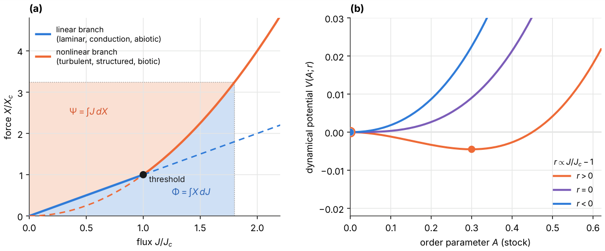
Figure 2.
The redox ladder versus soil moisture. Free energy per electron for the oxidation of organic matter ( V) with successive electron acceptors, from standard reduction potentials at pH 7, each drawn over the indicative soil-moisture range where it dominates; anoxic conditions are shaded. Pink: butyrate oxidation (per mol butyrate) is endergonic at standard conditions ( kJ ) and becomes exergonic only with an H2 consumer (open circle; 21 nM H2, M butyrate, M acetate).
Figure 2.
The redox ladder versus soil moisture. Free energy per electron for the oxidation of organic matter ( V) with successive electron acceptors, from standard reduction potentials at pH 7, each drawn over the indicative soil-moisture range where it dominates; anoxic conditions are shaded. Pink: butyrate oxidation (per mol butyrate) is endergonic at standard conditions ( kJ ) and becomes exergonic only with an H2 consumer (open circle; 21 nM H2, M butyrate, M acetate).
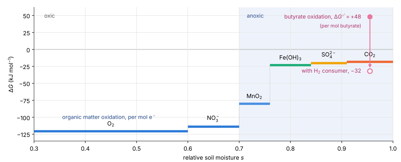
Figure 3.
Soil syntrophy. (a) Energy obtained per mole of butyrate by the oxidizer and by the methanogens; their sum (dashed) is independent of H2 (Equation (13)), and the shaded band is the window of Equation (12) (M butyrate, M acetate, atm, atm, pH 7, C). (b) Equilibrium H2 of Equation (14) without methanogens (, orange; dashed where unstable) and with them (, blue); green shading marks where the partner is indispensable, . (c) Equilibrium entropy production of the methanogens, Equation (15), and of the pair if all hydrogen derives from butyrate oxidation (dashed). Parameters: , , , M , , .
Figure 3.
Soil syntrophy. (a) Energy obtained per mole of butyrate by the oxidizer and by the methanogens; their sum (dashed) is independent of H2 (Equation (13)), and the shaded band is the window of Equation (12) (M butyrate, M acetate, atm, atm, pH 7, C). (b) Equilibrium H2 of Equation (14) without methanogens (, orange; dashed where unstable) and with them (, blue); green shading marks where the partner is indispensable, . (c) Equilibrium entropy production of the methanogens, Equation (15), and of the pair if all hydrogen derives from butyrate oxidation (dashed). Parameters: , , , M , , .
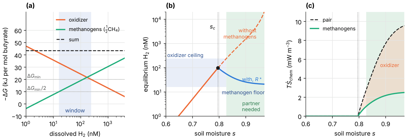
Figure 4.
The hydrologic cycle as an engine, after Konings et al. [43]. A water parcel evaporates at (1→2), mixes irreversibly into air of relative humidity h (2→3, dashed), rises dry-adiabatically to the lifting condensation level (3→LCL), condenses during moist ascent at a mean temperature (LCL→4→5), and returns as rain, warming to (5→1). The loop runs inside two reservoirs, column vapour Q and root-zone water , which exchange water with their surroundings through import , export , runoff and leakage K.
Figure 4.
The hydrologic cycle as an engine, after Konings et al. [43]. A water parcel evaporates at (1→2), mixes irreversibly into air of relative humidity h (2→3, dashed), rises dry-adiabatically to the lifting condensation level (3→LCL), condenses during moist ascent at a mean temperature (LCL→4→5), and returns as rain, warming to (5→1). The loop runs inside two reservoirs, column vapour Q and root-zone water , which exchange water with their surroundings through import , export , runoff and leakage K.
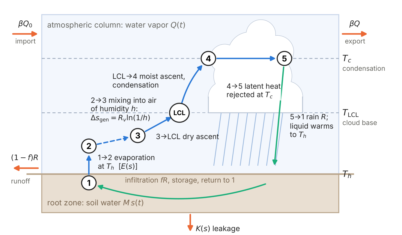
Figure 5.
The self-excited hydrologic engine. (a) Phase plane of Equations (16)–(): nullclines (dashed), unstable equilibrium (open circle) and limit cycle. Markers A–G are evaporation times along one period, coloured by the relative humidity h met at evaporation. (b) Soil moisture, column vapour and rainfall over two periods. (c) Temperature–entropy cycle of water evaporated at the time-mean surface state ( K, ), on the saturated-liquid and saturated-vapour curves of water (the entropy axis omits the two-phase region). Legs as in Figure 4. Shaded bands show the range of and along the orbit, from B, C (lowest) to F, G (highest). (d) Engine power, Equation (20): attainable , reversible , and the part spent lifting condensate, .
Figure 5.
The self-excited hydrologic engine. (a) Phase plane of Equations (16)–(): nullclines (dashed), unstable equilibrium (open circle) and limit cycle. Markers A–G are evaporation times along one period, coloured by the relative humidity h met at evaporation. (b) Soil moisture, column vapour and rainfall over two periods. (c) Temperature–entropy cycle of water evaporated at the time-mean surface state ( K, ), on the saturated-liquid and saturated-vapour curves of water (the entropy axis omits the two-phase region). Legs as in Figure 4. Shaded bands show the range of and along the orbit, from B, C (lowest) to F, G (highest). (d) Engine power, Equation (20): attainable , reversible , and the part spent lifting condensate, .
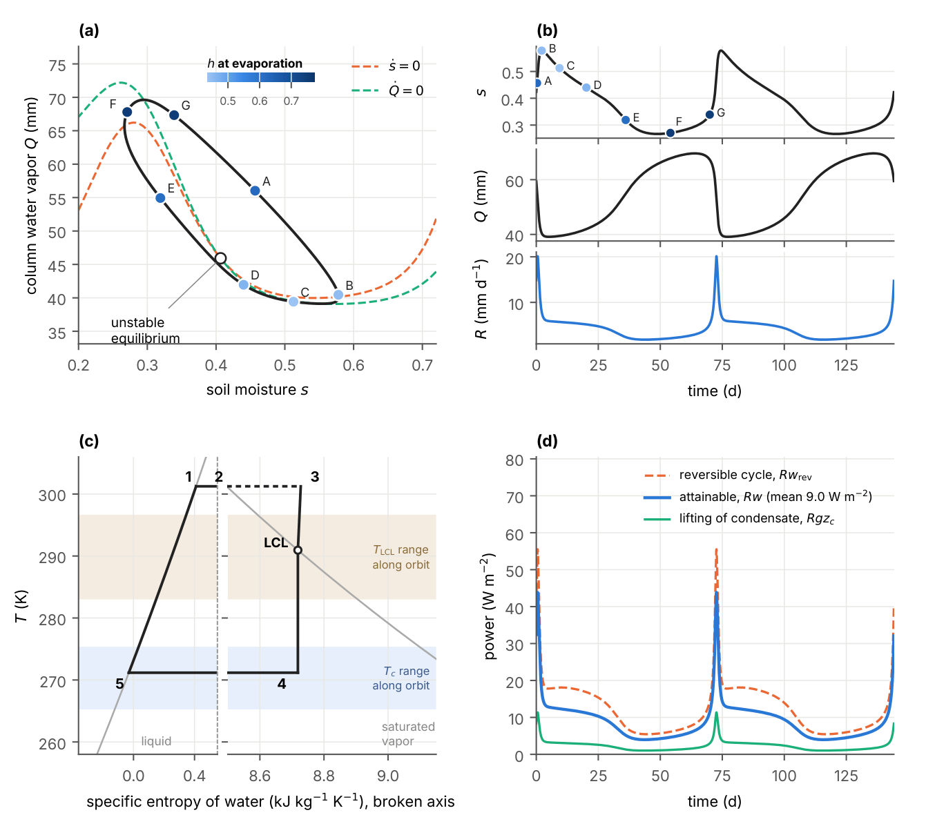
Figure 6.
The planet as a heat exchanger, 1850–2100. (a) Effective radiative forcing by component [66] and total anthropogenic forcing in three idealized futures from 2025 (dashed): CO2 emissions held at the 2024 level (purple), emissions that keep the CO2 concentration constant (red) and zero CO2 emissions (green). The futures are computed with the impulse response of [67], rescaled to the observed 2024 concentration, with non-CO2 forcing held at its 2024 value. (b) Observed warming [66] and the response of the two-reservoir model, Equation (21), driven by the total forcing, with reduced in proportion to F and decreasing with T so that emission rises by W ; dashed lines show the three futures. (c) Transient entropy budget, Equation (23), for the constant-concentration path (11-year running means): entropy stored in the reservoirs, change in the infrared export, and the resulting change in entropy production.
Figure 6.
The planet as a heat exchanger, 1850–2100. (a) Effective radiative forcing by component [66] and total anthropogenic forcing in three idealized futures from 2025 (dashed): CO2 emissions held at the 2024 level (purple), emissions that keep the CO2 concentration constant (red) and zero CO2 emissions (green). The futures are computed with the impulse response of [67], rescaled to the observed 2024 concentration, with non-CO2 forcing held at its 2024 value. (b) Observed warming [66] and the response of the two-reservoir model, Equation (21), driven by the total forcing, with reduced in proportion to F and decreasing with T so that emission rises by W ; dashed lines show the three futures. (c) Transient entropy budget, Equation (23), for the constant-concentration path (11-year running means): entropy stored in the reservoirs, change in the infrared export, and the resulting change in entropy production.
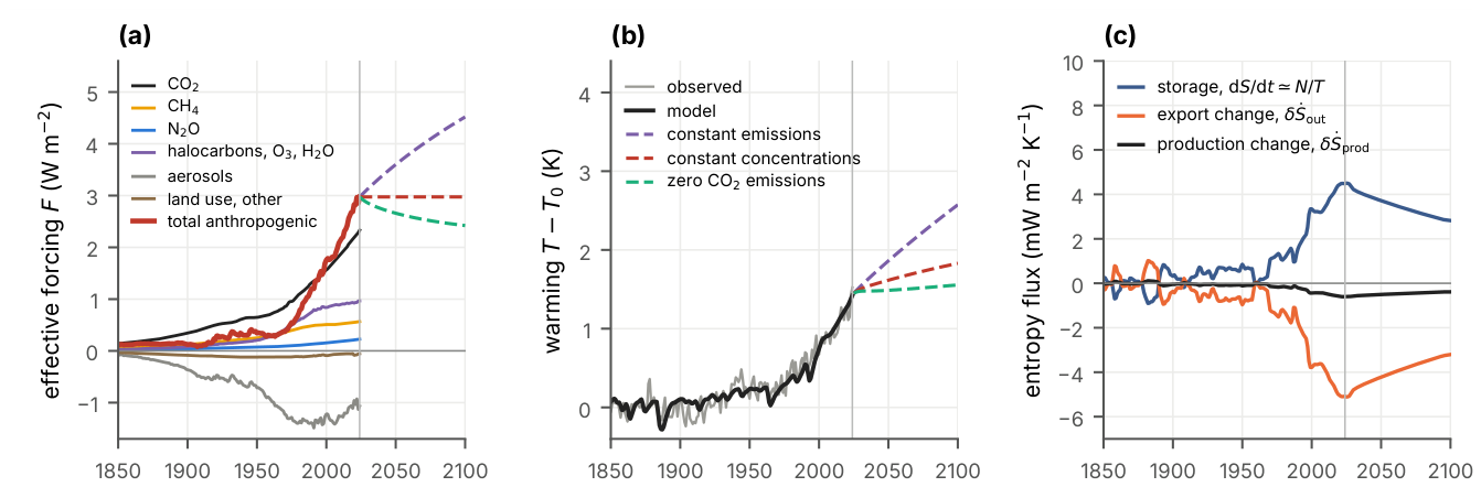
Figure 7.
From computation to the planet. (a) Energy per operation, from Landauer’s bound to a 16-bit floating-point operation at the facility level (top), and the energy trapped within a century by the CO2 emitted to supply that operation, for three electricity supplies (, and kg CO2 ; bottom), using the marginal forcing of CO2 at 420 ppm [80] and the carbon impulse response of [67]. (b) Land needed to supply data-centre demand from solar power with storage ( W , storage losses) for low, base and high demand paths (IEA cases [72], extended to 2050 at 0, 2 and per year), compared with the footprint of the data centres themselves ( W ).
Figure 7.
From computation to the planet. (a) Energy per operation, from Landauer’s bound to a 16-bit floating-point operation at the facility level (top), and the energy trapped within a century by the CO2 emitted to supply that operation, for three electricity supplies (, and kg CO2 ; bottom), using the marginal forcing of CO2 at 420 ppm [80] and the carbon impulse response of [67]. (b) Land needed to supply data-centre demand from solar power with storage ( W , storage losses) for low, base and high demand paths (IEA cases [72], extended to 2050 at 0, 2 and per year), compared with the footprint of the data centres themselves ( W ).
Disclaimer/Publisher’s Note: The statements, opinions and data contained in all publications are solely those of the individual author(s) and contributor(s) and not of MDPI and/or the editor(s). MDPI and/or the editor(s) disclaim responsibility for any injury to people or property resulting from any ideas, methods, instructions or products referred to in the content. |
© 2026 by the authors. Licensee MDPI, Basel, Switzerland. This article is an open access article distributed under the terms and conditions of the Creative Commons Attribution (CC BY) license (http://creativecommons.org/licenses/by/4.0/).
Copyright: This open access article is published under a Creative Commons CC BY 4.0 license, which permit the free download, distribution, and reuse, provided that the author and preprint are cited in any reuse.