

Submitted:
13 November 2026
Posted:
17 November 2026
You are already at the latest version
Abstract
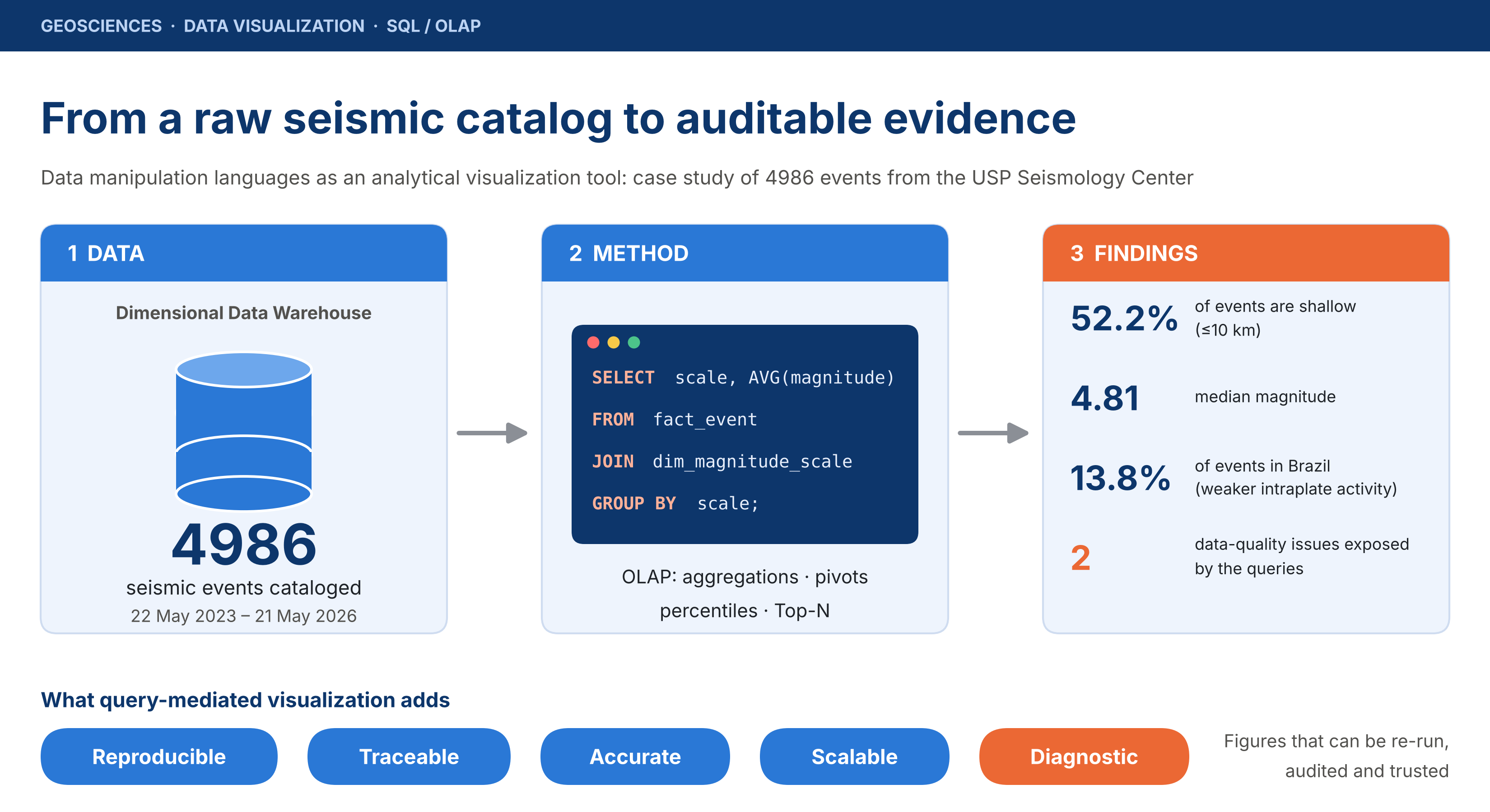
Background: Scientific figures are often treated as illustrations, although their evidential value depends on whether they can be traced to, and regenerated from, the underlying data. Methods: We evaluated a catalog of 4986 seismic events recorded by the Seismology Center of the University of São Paulo (USP) between 22 May 2023 and 21 May 2026, stored in a dimensional Data Warehouse and analyzed with SQL-based OLAP queries (aggregations by year, magnitude scale, region, weekday, semester and author; contingency tables; continuous percentiles; Top-N rankings). Results: The queries reproduced well-established seismological patterns: shallow events (≤10 km; 52.2%) of moderate to strong magnitude predominated (median 4.81), epicenters traced plate boundaries, and Brazilian intraplate events were weaker than international ones. The same queries exposed two data-quality problems: duplicated spellings of an author name and eight magnitude scales instead of the six defined in the model. Conclusions: Mediating visualization through data manipulation languages gives figures reproducibility, traceability, computational accuracy and, in principle, scalability, and adds a diagnostic capacity that purely illustrative charts lack. These languages are therefore a central methodological tool for environmental and geological data analysis, with reliability that remains conditional on the quality of data loading and modeling.
Keywords:
data warehouse
; SQL
; data visualization
; seismology
; OLAP
; data quality
; reproducibility
1. Introduction
The growing instrumentation of the planet and the resulting proliferation of geophysical sensors have turned geology and the environmental sciences into data-intensive domains. Seismic networks, weather stations, remote-sensing satellites and oceanographic buoys continuously produce volumes of records whose interpretation depends less and less on manual inspection and more and more on computational infrastructures able to store, integrate and summarize raw information. In this scenario, the frontier between observed data and scientific knowledge is occupied by a technological layer that is often invisible to the reader of a report: data manipulation languages.
This article departs from a concrete artifact, namely an analytical report produced from a Data Warehouse named TerremotosUSP, fed with 4986 seismic events cataloged by the Seismology Center of the University of São Paulo (USP) between 22 May 2023 and 21 May 2026, in order to examine two complementary research questions:
- RQ1 (descriptive). What do the data reveal about the physical behavior of the recorded earthquakes?
- RQ2 (methodological and epistemological; the central thesis of this work). To what extent can data manipulation languages, particularly SQL applied to the dimensional structure of a Data Warehouse, be sustained as a legitimate instrument and, it is argued here, one superior to merely illustrative alternatives for the visualization of scientific data in the geosciences?
The distinction is not trivial. A feature explicitly stated by the source report is that all of its charts were computed directly from the source data rather than built as approximate illustrations. This seemingly technical statement carries deep methodological implications: when a figure is the deterministic result of a declarative query over a versioned dataset, it ceases to be a rhetorical device and becomes a reproducible, auditable and falsifiable object, and these are the properties that scientific methodology demands of any empirical evidence [1,2].
The investigation is justified on three grounds. First, its applied relevance: understanding seismic risk and, by extension, related environmental phenomena depends on the ability to turn raw catalogs into interpretable syntheses. Second, its pedagogical relevance: technology and information-systems courses often teach SQL and dimensional modeling detached from real scientific applications, missing the opportunity to demonstrate their value as a method. Third, its epistemological relevance: discussing the chain that runs from raw data to the published figure is discussing the very reliability of scientific evidence in the era of large data volumes.
The general objective of this article is to evaluate the USP seismic catalog and, on that basis, to support the use of data manipulation languages as an analytical visualization tool in the geosciences. The specific objectives are to: (i) describe the physical behavior of the events in terms of magnitude, depth, and temporal and spatial distribution; (ii) systematize the results of the analytical (OLAP) queries documented in the project; (iii) identify data-quality problems evidenced by the analysis; and (iv) critically discuss the methodological properties (reproducibility, traceability, accuracy and scalability) that mediation by query languages confers on scientific visualization.
The remainder of the article is organized as follows. Section 2 establishes the theoretical background on databases, analytical processing, visualization and seismology. Section 3 details the materials and methods. Section 4 presents the results, Section 5 discusses them in light of the central thesis and its limitations, and Section 6 draws the conclusions.
2. Theoretical Background
This section gathers the conceptual foundations that support the analysis. It discusses, in sequence, the relational model and the SQL language, the Data Warehouse architecture and OLAP processing, the principles of quantitative data visualization and reproducibility, and, finally, the elementary notions of seismology required to interpret the catalog.
2.1. The Relational Model and the SQL Language
The conceptual basis of structured data manipulation was established by Codd [3], who proposed the relational model as a way of organizing information in relations (tables) free from the physical-access dependencies that characterized earlier systems. The main contribution of the model was to separate the specification of what is wanted from the way the system obtains it, inaugurating the declarative paradigm that the SQL language would later consolidate. Date [4] and Elmasri and Navathe [5] systematize this heritage, stressing that the underlying relational algebra gives queries a precise semantics: given the same database state, a query always produces the same result.
This determinism is decisive for the argument defended here. Unlike a manual counting procedure or a visual estimate, an SQL aggregation query (a GROUP BY clause combined with functions such as COUNT, AVG or PERCENTILE_CONT) is a formal specification whose result can be re-executed by any researcher and independently verified. The language thus works not only as an operational tool but also as a methodological record of the analytical reasoning itself.
2.2. Data Warehouse, Dimensional Modeling and OLAP
Operational databases are optimized for transactions; the analysis of large historical records requires a distinct architecture. Inmon [6] defined the Data Warehouse as a subject-oriented, integrated, non-volatile and time-variant collection of data intended to support decisions. Kimball and Ross [7] complement this view with dimensional modeling, in which data are organized in a fact table, which stores the quantitative measures of the events, surrounded by dimension tables that provide the descriptive contexts (time, location, measurement scale, authorship) by which facts can be filtered and aggregated.
On this structure operates online analytical processing (OLAP), whose reference characterization was given by Chaudhuri and Dayal [8]. Typical operations (drill-down, roll-up, slice, dice and pivoting) are ways of navigating the dimensions and summarizing the measures at different granularities. Gray et al. [9] showed how such operations can be expressed within SQL by generalizing GROUP BY into the data-cube operator, which unifies histograms, cross-tabulations and sub-totals. In the case examined here, each documented query (referred to in the project as Q1 to Q4, besides pivots, percentile analyses and Top-N operators) is an instance of these operations, and each figure of the report is the visual projection of a data cube obtained by aggregation.
It is worth stressing that dimensional modeling is itself a quality instrument. Data quality is a multidimensional concept that includes, among others, accuracy and consistency of representation [10]; by making dimensions such as magnitude-scale type and authorship explicit, the model renders visible inconsistencies that would remain hidden in unstructured storage. As Section 4 shows, it was precisely the scale dimension that exposed the existence of unforeseen measurement types.
2.3. Visualization of Quantitative Data and Reproducibility
Scientific visualization is not ornament but argument. Tufte [11] formulated principles that are now classic: maximize the data-ink ratio, avoid graphical distortion and privilege the integrity of the representation over decorative effect. Few [12] extends these principles to the contemporary analytical context, emphasizing that the choice of chart type must derive from the nature of the question and the structure of the data, not from arbitrary aesthetic preferences.
A central point of these authors, frequently underestimated, is provenance: a graph is scientifically defensible only if it can be traced back to the data that originated it. This echoes the broader reproducible-research agenda, which treats the availability of code and data as a minimum standard for assessing computational claims [1], and the practical recommendations to keep track of how every result was produced, to avoid manual data-manipulation steps and to always store the raw data behind plots [2]. The FAIR principles (findable, accessible, interoperable and reusable data) complete this picture from the data-stewardship side [13]. Code-based visualization tools, such as the Matplotlib library [14], the Python data-analysis ecosystem structured around the pandas library [15] and the grammar of graphics implemented by Wickham [16], realize this principle by inseparably coupling the transformation of the data to its representation. When the same routine that queries the database generates the figure, the distance between evidence and representation is reduced to zero.
2.4. Fundamentals of Seismology
Earthquakes result from the abrupt release of energy accumulated in geological faults, mostly concentrated at the boundaries of tectonic plates. Magnitude quantifies the released energy on a logarithmic scale; the depth of the focus (hypocenter) distinguishes shallow, intermediate and deep events, the latter typical of subduction zones, where one plate plunges beneath another. Different magnitude scales, such as the local magnitude of Richter [17] and the moment magnitude of Hanks and Kanamori [18], are calibrated to distinct ranges and wave types and are therefore not directly interchangeable. The statistical relation by which large events are exponentially rarer than small ones was established by Gutenberg and Richter [19] and remains a reference for assessing the plausibility of a catalog.
The Brazilian territory lies in the stable interior of the South American plate, a setting classified as intraplate and characterized by low-magnitude seismicity and lower energy release than plate-boundary regions such as the Andes and the Pacific Ring of Fire; in this mid-plate setting, the stress field varies in nature and orientation [20]. This distinction is central to interpreting the comparison between Brazilian and international events presented in the catalog.
3. Materials and Methods
This research is a case study of a quantitative, descriptive nature with an applied purpose. The empirical object is the graphical-analysis report of the TerremotosUSP Data Warehouse, and the strategy consists in interpreting its results as simultaneous evidence of two orders: about the seismic phenomenon and about the computational method that produced the evidence.
3.1. Data Source and Scope
The data come from the Seismology Center of USP and comprise 4986 seismic events recorded between 22 May 2023 and 21 May 2026. The catalog is global, not restricted to Brazilian territory, and each record carries, at a minimum, the attributes of date and time, epicenter latitude and longitude, depth, magnitude, type of measurement scale, named geographic region and cataloging author. Table 1 summarizes the key figures of the dataset.
3.2. Analytical Architecture
The data were organized in a dimensionally modeled Data Warehouse (Figure 1), with a fact table storing the event measures (magnitude and depth) and descriptive dimensions of time, location, magnitude scale and authorship (Figure 2). On this structure, a set of analytical queries was specified in SQL, ranging from simple aggregations to continuous statistical operations. The queries were then parameterized in routines that, besides returning the result tables, directly generated the corresponding figures, ensuring that each chart displayed values effectively computed over the full dataset rather than samples or estimates.
3.3. Analytical Queries and Visualizations
The source report reproduces and comments on fourteen figures grouped in three blocks. The first describes the physical behavior of the events (magnitude, depth, temporal evolution, geographic distribution and the magnitude–depth relation). The second materializes the formal OLAP queries: mean magnitude by year and scale (Q1), regions with the greatest mean depth (Q2), frequency by weekday and semester (Q3), production by author and year (Q4), a year-by-quarter contingency table (pivoting), magnitude percentiles by year, and a ranking of the largest events (Top-N). The third block gathers additional comparisons between Brazilian and international events and the dispersion of the measurement scales. Table 2 catalogs the queries and indicates where their results are reported. In the present article, the numerical outputs of these queries are reported in the text and in Table 1, Table 3 and Table 4, and the graphical outputs are presented in Figure 3, Figure 4, Figure 5, Figure 6, Figure 7, Figure 8, Figure 9, Figure 10, Figure 11, Figure 12, Figure 13, Figure 14 and Figure 15. These are the figures of the source report, generated directly from the full dataset, with titles and axis labels translated into English; the Top-N chart is not repeated because Table 4 reports the same information. Figure 1 and Figure 2 are conceptual diagrams prepared for this article.
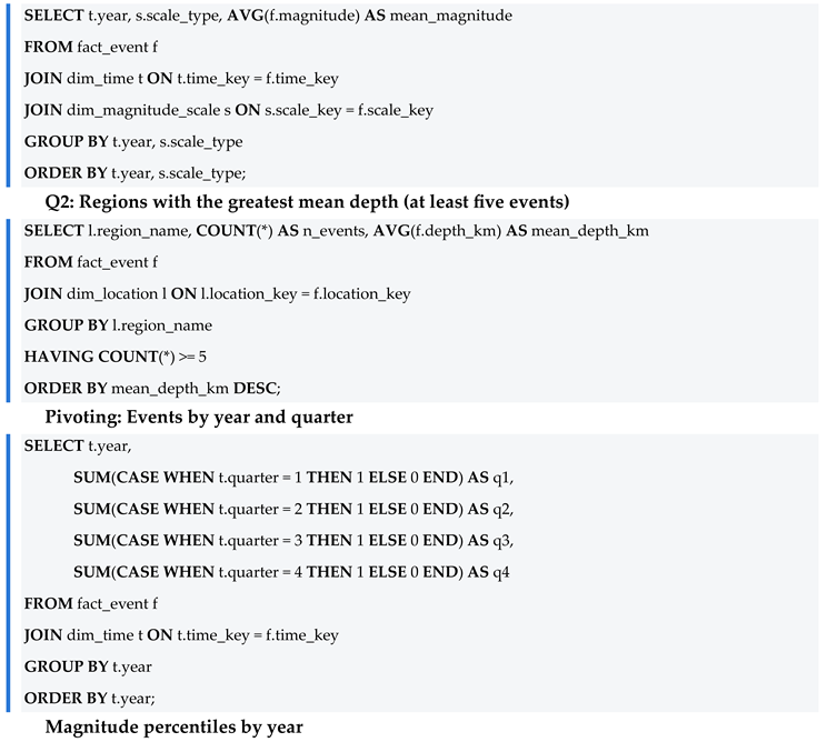
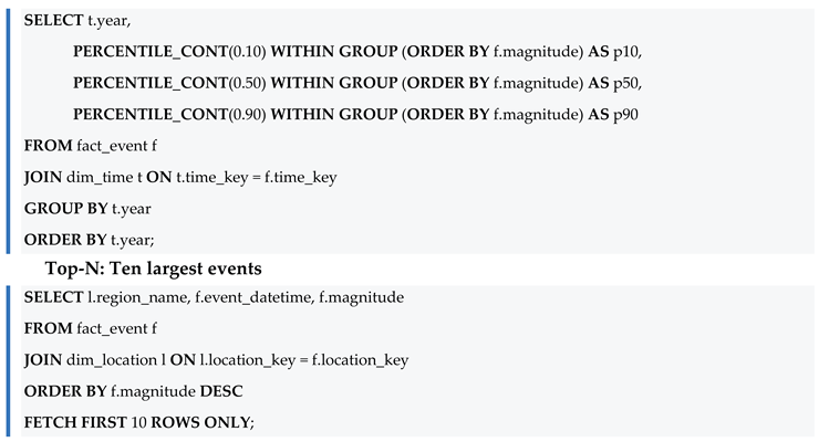
Illustrative SQL sketches of the main query patterns are given in Appendix A.
3.4. Analytical Framework
The interpretation crosses the observed results with the theoretical expectations of seismology (Section 2.4) and, in parallel, evaluates the methodological properties of the figure-production chain along four criteria: (i) reproducibility, the ability of any researcher with the same dataset and query to obtain the same figure; (ii) traceability, the ability to follow each figure back to the query and the data that originated it; (iii) computational accuracy, the guarantee that the displayed values are computed over the full dataset with the declared statistical construct; and (iv) scalability, the invariance of the analytical logic with respect to data volume. A fifth attribute, diagnostic capacity, is considered: the ability of the queries to expose inconsistencies in the data themselves.
3.5. Use of Generative AI Tools
Generative AI was used in the preparation of this manuscript for support in translation from Portuguese into English, language editing, restructuring to the preprint format, drafting of explanatory text (Table 2, Table 5 and Table 6 and Appendix A), preparation of the conceptual Figure 1 and Figure 2 and of the graphical abstract, translation of the titles and axis labels of Figure 3, Figure 4, Figure 5, Figure 6, Figure 7, Figure 8, Figure 9, Figure 10, Figure 11, Figure 12, Figure 13, Figure 14 and Figure 15 from Portuguese into English, and drafting of the text that accompanies Figure 3, Figure 4, Figure 5, Figure 6, Figure 7, Figure 8, Figure 9, Figure 10, Figure 11, Figure 12, Figure 13, Figure 14 and Figure 15, including approximate values read from the charts, which are indicated as such. The data content of Figure 3, Figure 4, Figure 5, Figure 6, Figure 7, Figure 8, Figure 9, Figure 10, Figure 11, Figure 12, Figure 13, Figure 14 and Figure 15 was not altered. The author reviewed and edited the outputs and is fully responsible for the content (see the Use of Generative AI Statement).
4. Results
The results are presented in the logical order of the analysis: first the physical overview of the events, then the formal analytical queries and the complementary comparisons and, finally, the data-quality findings that connect the observations to the methodological discussion in Section 5.
4.1. Physical Overview of the Events
4.1.1. Magnitude
The magnitude distribution is markedly concentrated in the moderate (4 to 5) and strong (5 to 6) ranges, with a median of 4.81 (Figure 3, left). The histogram is bimodal: the main mode peaks at about magnitude 5, whereas a smaller secondary mode appears around magnitude 2 to 2.5. The classification by classes (Figure 3, right) reveals 2291 moderate and 1690 strong events, against only 192 events classified as great (magnitude ≥ 6), 158 minor events (3 to 4) and 655 microearthquakes (magnitude below 3). The secondary mode deserves attention: the number of microearthquakes (655) is close to the number of events located in Brazil (689; Section 4.3.1), and the median magnitude of the Brazilian events (about 2.2) falls precisely in this range. This suggests, although the aggregated results shown here do not prove it, that the low-magnitude mode is largely formed by Brazilian events. The rarity of great events is consistent with the Gutenberg–Richter relation [19]: frequency decays exponentially with increasing magnitude, so that consistent catalogs should exhibit few large events relative to moderate ones. The decline in counts below magnitude 5 reflects the incomplete detection of smaller events in a global catalog, so the relation applies only above the completeness magnitude; from the strong (5 to 6) to the great (≥ 6) class, the ratio of about 9 to 1 is close to the decay of one order of magnitude per unit of magnitude that is typical of the relation. The upper part of the distribution therefore also works as a plausibility test of the catalog itself, which it passed in this case.
4.1.2. Depth
About 52% of the events are shallow (depth ≤ 10 km), with 2603 records in this range against 715 in the 10–70 km range, 1544 in the intermediate 70–300 km range and 124 deep events (beyond 300 km) (Figure 4, right). The histogram (Figure 4, left, limited to 350 km for readability) shows that the shallow class is dominated by the first two 10-km bins, with roughly 790 and 1880 events, respectively, followed by a long tail of much smaller counts that decays between about 100 and 250 km. The very high count in the second bin may reflect events whose depth is not resolved and is assigned a conventional value, a possibility that deserves verification in the source data. Many shallow records have a depth equal to zero, flagged by the Center itself as an indication of a shallow event without a precise depth. This is a relevant methodological detail, since a null value should not be interpreted as an exact measurement but as a marker of indeterminacy. The tail of deep events, although a minority, is physically significant: it corresponds to subduction zones, where the plunging plate generates deep-focus earthquakes.
4.1.3. Temporal Evolution
The monthly series (Figure 5, left) is relatively stable around a mean of approximately 135 events per month (4986 events over 37 calendar months, counting the two partial months), with a maximum of roughly 187 events in a single month, and the cumulative curve (Figure 5, right) grows almost linearly until it reaches the 4986 records. The lowest values, at the two ends of the series (about 50 events in the first month and about 84 in the last), correspond to the partial months of May 2023 and May 2026. The years 2024 and 2025 appear complete, whereas 2023 and 2026 are partial, since collection begins in May 2023 and ends in May 2026. This detail is crucial for the correct reading of the annual aggregations: lower totals in 2023 and 2026 reflect incomplete observation windows, not a real variation in seismic activity. The distinction between variation of the phenomenon and sampling artifact is precisely the kind of discernment that the temporal structuring of the Data Warehouse makes possible (see also Section 4.2.5).
4.1.4. Geographic Distribution
The global map of epicenters (Figure 6) sharply outlines the boundaries of the tectonic plates: the Andes, the South Sandwich Islands, the Mid-Atlantic Ridge and the Pacific Ring of Fire (Japan, the Philippines, Kamchatka). Over Brazilian territory, a cluster of pale, low-magnitude events forms, visibly less energetic than those at plate boundaries, where the darker and larger symbols concentrate. The correspondence between the observed distribution and plate tectonics is strong and serves, once more, as cross-validation: a catalog whose epicenters did not reproduce the known plate boundaries would be immediately suspect.
4.1.5. Magnitude–Depth Relation
The joint density of magnitude and depth, represented on a logarithmic scale (Figure 7), concentrates in shallow events of magnitude 4 to 6. The plot also shows a distinct column of events at near-zero depth with magnitudes between about 1 and 3, which is consistent with the Brazilian events discussed in Section 4.3.1, and indicates that, below magnitude 4, events at greater depths are very rare, as expected for a global catalog whose detection capability decreases for small distant earthquakes. No strong correlation between depth and magnitude is observed, although very deep events tend to present intermediate-to-high magnitudes. The absence of a simple linear correlation reinforces the importance of multivariate analyses and discourages naive inferences. This is a methodological warning that only becomes evident when the data are examined jointly rather than in isolated cuts.
4.2. Analytical (OLAP) Queries
4.2.1. Q1: Mean Magnitude by Year and Scale
Segmenting mean magnitude by year and by measurement scale (Figure 8) shows that the scales differ strongly in the level of magnitude they report. The mB scale records the highest means (approximately 5.7 to 6.3, with no mB events in 2026), followed by mb (approximately 4.8 to 4.9 in every year), whereas the mR (approximately 2.3 to 2.5) and MLv (approximately 1.6 to 2.1, decreasing over the years) scales report much lower values. The values quoted here are read from the chart and are therefore approximate. This pattern is expected from an instrumental standpoint, since each scale is calibrated for distinct ranges and wave types, and it is consistent with the use of regional and local scales for small nearby events and of body-wave scales for larger distant ones. The finding illustrates why the magnitude-type dimension is indispensable: comparing magnitudes without controlling for the measurement scale would produce spurious conclusions. By crossing the measure with the appropriate dimension, the query converts a risk of interpretive error into an explicit control.
4.2.2. Q2: Regions with the Greatest Mean Depth
Considering only regions with at least five events (Figure 9), the province of Santiago del Estero, in Argentina, leads with a mean depth of approximately 487 km (15 events), followed by the Fiji Islands region (449 km; 22 events), the Bonin Islands region of Japan (365 km; 12 events) and the south of the Fiji Islands (351 km; 8 events). Western Brazil also appears in the ranking (305 km; 5 events), as do several regions along the Andean margin and the Mariana Islands. Most of these regions correspond to subduction zones, in which the plate plunges and generates deep-focus earthquakes; in the case of western Brazil, the depth is more plausibly related to the slab beneath western South America than to shallow intraplate seismicity, an interpretation that would require confirmation with the event-level data. The filter on the minimum number of events is here a relevant statistical safeguard: without it, regions with a single deep record could head the ranking in a misleading way. The filtering clause, trivial in SQL and laborious manually, protects the analysis against the noise of small samples.
4.2.3. Q3: Frequency by Weekday and Semester
The distribution of events across the days of the week is practically uniform (Figure 10, left), oscillating around a mean of 712 events per weekday; the chart suggests a maximum of about 750 events on Tuesdays and a minimum of about 665 on Wednesdays, and the two semesters present close counts, 2460 and 2526 (Figure 10, right). Uniformity is exactly what is expected of a natural phenomenon with no link to the human calendar; small variations reflect only sampling chance. This seemingly banal result fulfills an important epistemological function: it constitutes a successful negative test, that is, the absence of a spurious pattern that, if present, would indicate a collection error or recording bias.
4.2.4. Q4: Production by Author and Year
Cataloging is concentrated in a few analysts: the identifications cleusa and jroberto account for most of the records (2540 and 1651, respectively), followed by JAlexandre (629) and a tail of four minor contributors with 104, 53, 8 and 1 events (Figure 11). The stacked bars add the temporal dimension requested by the query: cleusa is present in all four years, with its largest share in 2024, jroberto concentrates most of its records in 2025, and JAlexandre appears only from 2024 onwards (approximate readings of the chart). In this query a data-quality problem emerged: the spellings J.Alexandre and JAlexandre represent the same author and had to be unified in the analysis. This is an inconsistency of origin that should be standardized when the authorship dimension is loaded. The episode is exemplary: it was the dimensional structuring itself, by grouping by author, that made the defect visible and measurable.
4.2.5. Pivoting: Events by Year and Quarter
The contingency table crossing year (rows) and quarter (columns) confirms, in the form of a heat map (Figure 12), the temporal pattern already identified: 2023 shows events only from the second quarter onward and 2026 only up to the second quarter, whereas 2024 and 2025 are evenly distributed over the four quarters (Table 3). The darkest cell is the second quarter of 2024 (484 events) and the lightest is the partial second quarter of 2023 (179 events), whereas the third and fourth quarters of 2025 are equal (435 events each). Pivoting is a canonical OLAP operation, and its visual reading shows how a single contingency query replaces, with greater clarity, dozens of manual counts.
4.2.6. Magnitude Percentiles by Year
The analysis of continuous percentiles (the PERCENTILE_CONT function; Figure 13) reveals that the median magnitude remains stable between approximately 4.75 and 4.9 across the years, while the 90th percentile (P90) stays around 5.5 to 5.8 and the 10th percentile (P10) lies between approximately 2.3 and 3.2, rising in 2026. The values are read from the chart and are therefore approximate. The range between P10 and P90 thus covers most events, from magnitudes of roughly 2.5 to 5.6. A higher P10 in the partial 2026 window may indicate a smaller share of low-magnitude events in that period, a hypothesis that could be tested in a follow-up analysis. This is a view that is robust to extreme values, which the mean alone would not offer. The choice of percentiles in place of means is a deliberate statistical decision, and the fact that it is expressed in a single window function highlights the expressiveness of the language: sophisticated statistical concepts become readable, re-executable clauses.
4.2.7. Top-N: Largest Earthquakes of the Period
The ranking operator applied to the catalog identifies the ten largest events of the period, headed by a magnitude 7.58 earthquake north of Honduras (8 February 2025), followed by events near the east coast of Kamchatka (7.51) and in Mindanao, Philippines (7.50). All of the largest events occurred at plate boundaries (mostly along the Pacific Ring of Fire, but also in the Caribbean, north of Honduras, and in continental Southeast Asia, Myanmar) and none in Brazilian territory, in full agreement with the low intraplate seismic energy of Brazil. Table 4 presents the complete ranking.
4.3. Additional Comparisons
4.3.1. Brazil and the International Scenario
Brazil accounts for 689 events, equivalent to 13.8% of the catalog, against 4297 international events (86.2%) (Figure 14, left). The box plots (Figure 14, right) show that the Brazilian median magnitude (about 2.2, with the central half of the events between about 1.9 and 2.5) is far lower than the international one (about 4.9, with the central half between about 4.5 and 5.3), and that the two ranges practically do not overlap: the upper whisker for Brazil (about 3.4) coincides with the lower whisker for the international events. These values are read from the chart and are therefore approximate. The result confirms that the country, located in the stable interior of the South American plate, records weaker earthquakes than plate-boundary regions, and it quantitatively materializes the theoretical distinction between intraplate and plate-boundary seismicity discussed in Section 2.4. Part of the difference may also reflect the fact that small events are only detected when they occur close to the stations of the Brazilian network, a factor that should be considered when comparing the two groups.
4.3.2. Magnitude Scales and Annual Stability
The count by measurement scale identified eight distinct scales (Figure 15, left), with an absolute predominance of the mb scale (3898 events), followed by mR (598), mB (286), MLv (134), Mw(mB) (42), M (23), Mw(Mwp) (3) and Mwp (2). The finding is methodologically relevant because two more scales, Mw(Mwp) and Mwp, were found than the six foreseen in the original dimensional model, suggesting the need to revise the loading of the magnitude-type dimension. The annual box plots (Figure 15, right) show very similar distributions between 2023 and 2026, with medians between approximately 4.75 and 4.9 and whiskers spanning roughly 2.9 to 6.7, indicating the stability of the catalog over time. Once again, it is the structured aggregation that turns a silent defect into actionable information.
4.4. Data-Quality Findings
Besides describing the phenomenon, the queries exposed four situations that require attention in the interpretation or in the data pipeline. Table 5 consolidates them together with the stage at which each was detected and a suggested remediation.
5. Discussion
5.1. Data Manipulation Languages as an Instrument of Visualization
The results of the previous sections allow the central thesis of this article to be sustained in a grounded way. It is argued that mediation by data manipulation languages confers on scientific visualization in the geosciences four properties that illustrative graphics do not possess, and that these properties are precisely those demanded by the scientific method (Table 6).
The first property is reproducibility. Each analyzed figure is the deterministic output of a query over a versioned dataset: any researcher in possession of the same database and the same query will obtain the same figure. This characteristic aligns the production of graphics with the reproducibility criterion that is now considered central to research integrity [1,2]. A graph drawn by hand or estimated visually offers no such guarantee.
The second property is traceability, or provenance. As Tufte [11] and Few [12] stress, a graph is scientifically defensible only if it can be traced back to the data that originated it. When the same routine that queries the Data Warehouse generates the figure, as happens in the libraries discussed by Hunter [14] and McKinney [15], the distance between evidence and representation is reduced to a minimum, and the causal chain from data to figure becomes auditable at every step.
The third property is computational accuracy. The source report is emphatic that the graphics were computed directly on the data rather than built as illustrations. This accuracy manifests in details that would be impractical manually: continuous percentiles computed by window function, filters on the minimum number of events that protect against small samples, and cross aggregations in contingency tables [9]. The language not only speeds up the calculation; it guarantees that the calculation is the correct and the declared one.
The fourth property is scalability. The same query that summarizes 4986 events would be expected to summarize, without any change of logic, a catalog ten or a hundred times larger. In a domain such as the geosciences, where data volumes grow continuously with the densification of sensor networks, this invariance of logic with respect to volume is a decisive methodological advantage: what changes is the data; the instrument remains. This property is argued from the structure of the approach and was not benchmarked in the present study.
There is, furthermore, a benefit that transcends the four properties and that the results showed in a particularly eloquent way: diagnostic capacity. It was the aggregation queries themselves that exposed the data-quality problems of the catalog, namely the duplicated spelling of authors and the magnitude scales beyond those foreseen (Table 5). The dimensional structuring and the query language thus functioned not only as a means of describing the phenomenon but as a mechanism of critique of the data themselves. An illustrative chart would never have revealed such inconsistencies, because it would be born already filtered by the aesthetic intention of whoever draws it.
5.2. Limitations
The limits of the argument must be acknowledged. The reliability of visualizations produced by data manipulation languages is conditional on the quality of loading and modeling: a correct query over poorly integrated data produces a precise figure of wrong information. The case of depth equal to zero, which signals indeterminacy rather than an exact measurement, illustrates that human interpretation remains indispensable. The language guarantees the fidelity between data and figure; it does not replace judgment about the meaning of the data. It is therefore a powerful instrument that expands, without dispensing with, the interpretive competence of the scientist.
Other limitations concern the design of the study. It is a single case study based on one institutional catalog and a three-year observation window, which is short for statistical analyses such as the Gutenberg–Richter relation. The superiority of query-mediated visualization over illustrative alternatives is argued from the properties of the method and from the evidence of the case; no controlled comparison between workflows was performed. Scalability was not benchmarked. Finally, the raw catalog is institutionally owned, so full replication requires access to the original data (see the Data Availability Statement).
5.3. Implications and Future Work
For practice, the findings recommend standardizing the authorship and magnitude-scale dimensions when the Data Warehouse is loaded, treating zero depth as an indeterminacy marker, and reporting annual aggregates together with their observation windows. For research, they suggest publishing the queries and result tables alongside the figures, in line with the FAIR principles [13]. For teaching, the case shows that SQL and dimensional modeling can be taught as scientific methods and not only as software skills. Future work should incorporate multivariate analyses and more sophisticated time-series techniques and extend the framework to other environmental domains (climatological, hydrological and oceanographic) in order to test the generality of the approach for the geosciences as a whole.
6. Conclusions
This article evaluated a catalog of 4986 seismic events recorded by the USP Seismology Center between May 2023 and May 2026 and, on that basis, sustained the thesis that data manipulation languages constitute a legitimate and advantageous scientific instrument for analytical visualization in the geosciences.
On the descriptive plane, the analysis confirmed patterns consolidated in the literature: the predominance of shallow events of moderate to strong magnitude, with a median of 4.81 and rare great events in conformity with the Gutenberg–Richter relation; the alignment of epicenters with tectonic plate boundaries; the concentration of the deepest events in subduction zones; and the lower energy release in the Brazilian intraplate setting, which accounts for only 13.8% of the records and for median magnitudes below the international ones. It also confirmed the temporal stability of the catalog and the need for careful reading of the partial windows of 2023 and 2026.
On the methodological plane, it was shown that mediation by SQL over a dimensional Data Warehouse, together with code-based visualization libraries, gives the figures reproducibility, traceability, computational accuracy and, in principle, scalability, besides a remarkable diagnostic capacity, evidenced by the detection of two data-quality flaws: duplicated authorship and unforeseen magnitude scales. These properties qualify data manipulation languages not as mere operational utilities but as components of the scientific method applied to the analysis of geological and environmental data.
Author Contributions
Conceptualization, M.A.A.; methodology, M.A.A.; software, M.A.A.; validation, M.A.A.; formal analysis, M.A.A.; investigation, M.A.A.; data curation, M.A.A.; writing (original draft preparation), M.A.A.; writing (review and editing), M.A.A.; visualization, M.A.A. The author has read and agreed to the submitted version of the manuscript.
Funding
This research received no external funding.
Institutional Review Board Statement
Not applicable. The study involved no humans or animals.
Informed Consent Statement
Not applicable.
Data Availability Statement
The seismic data analyzed in this article come from the TerremotosUSP Data Warehouse, structured from the catalog maintained by the Seismology Center of the University of São Paulo (USP). The raw dataset is institutionally owned by the USP Seismology Center, and full access must be requested directly from that institution. The aggregated tables, the documented analytical (SQL) queries and the summarized results that underpin the figures and tables of this article can be made available by the author upon reasonable request sent by e-mail, for purposes of verification and reproduction of the results.
Acknowledgments
I would like to express my gratitude to Prof. Me. Pedro Antônio Galvão Júnior, professor of Database Systems (Modules I and II) at Fatec Dr. Bernardino de Campos, who guided me throughout the coursework to complete the code and refine the documentation that evolved into this paper. My acknowledgments go to Prof. Dr. Tung Chiun Wen for his scientific advice on how to conduct the research according to rigorous scientific standards; to the Director of Fatec Dr. Bernardino de Campos, Prof. Dr. João Roberto Maiellaro, for encouraging me and reiterating the importance of pursuing publication; and to my esteemed colleague Mr. Valdecir Dias Vieira, who accompanied me in discussions regarding the maturation of the scientific submission theme over many hours of tea.
Conflicts of Interest
The author declares no conflicts of interest of any nature (financial, commercial, professional, academic or personal) that could have influenced the conduct of this research or the interpretation of its results. The study received no funding from funding agencies or public or private institutions, and there is no link between the author and the Seismology Center of the University of São Paulo other than the use of the data it makes publicly available for academic purposes.
Use of Generative AI Statement
During the preparation of this manuscript, the author used Claude Sonnet 5.5 (Anthropic) for support in translation from Portuguese into English, language editing, restructuring to the preprint format, drafting of explanatory text (Table 2, Table 5 and Table 6, Appendix A and the text that accompanies Figure 3, Figure 4, Figure 5, Figure 6, Figure 7, Figure 8, Figure 9, Figure 10, Figure 11, Figure 12, Figure 13, Figure 14 and Figure 15), edition of Figure 1 and Figure 2 and the graphical abstract, and translation of the titles and axis labels of Figure 3, Figure 4, Figure 5, Figure 6, Figure 7, Figure 8, Figure 9, Figure 10, Figure 11, Figure 12, Figure 13, Figure 14 and Figure 15 from Portuguese into English. The author reviewed and edited substantially the outputs and takes full responsibility for the content of this publication.
Appendix A. Illustrative SQL Patterns
The sketches below illustrate the query patterns behind the analyses of Section 4. They are written in ANSI-style SQL with generic table and column names and may differ from the production schema; the syntax of ordered-set aggregates (PERCENTILE_CONT) and of row limiting varies among database engines.
Q1: Mean magnitude by year and magnitude scale
References
- Peng, R.D. Reproducible research in computational science. Science 2011, 334, 1226–1227. [Google Scholar] [CrossRef]
- Sandve, G.K.; Nekrutenko, A.; Taylor, J.; Hovig, E. Ten simple rules for reproducible computational research. PLoS Comput. Biol. 2013, 9, e1003285. [Google Scholar] [CrossRef]
- Codd, E.F. A relational model of data for large shared data banks. Commun. ACM 1970, 13, 377–387. [Google Scholar] [CrossRef]
- Date, C.J. An Introduction to Database Systems, 8th ed.; Addison-Wesley: Boston, MA, USA, 2003. [Google Scholar]
- Elmasri, R.; Navathe, S.B. Fundamentals of Database Systems, 7th ed.; Pearson: Hoboken, NJ, USA, 2016. [Google Scholar]
- Inmon, W.H. Building the Data Warehouse, 4th ed.; Wiley: Indianapolis, IN, USA, 2005. [Google Scholar]
- Kimball, R.; Ross, M. The Data Warehouse Toolkit: The Definitive Guide to Dimensional Modeling, 3rd ed.; Wiley: Indianapolis, IN, USA, 2013. [Google Scholar]
- Chaudhuri, S.; Dayal, U. An overview of data warehousing and OLAP technology. ACM SIGMOD Rec. 1997, 26, 65–74. [Google Scholar] [CrossRef]
- Gray, J.; Chaudhuri, S.; Bosworth, A.; Layman, A.; Reichart, D.; Venkatrao, M.; Pellow, F.; Pirahesh, H. Data cube: A relational aggregation operator generalizing group-by, cross-tab, and sub-totals. Data Min. Knowl. Discov. 1997, 1, 29–53. [Google Scholar] [CrossRef]
- Wang, R.Y.; Strong, D.M. Beyond accuracy: What data quality means to data consumers. J. Manag. Inf. Syst. 1996, 12, 5–33. [Google Scholar] [CrossRef]
- Tufte, E.R. The Visual Display of Quantitative Information, 2nd ed.; Graphics Press: Cheshire, CT, USA, 2001. [Google Scholar]
- Few, S. Show Me the Numbers: Designing Tables and Graphs to Enlighten, 2nd ed.; Analytics Press: Burlingame, CA, USA, 2012. [Google Scholar]
- Wilkinson, M.D.; Dumontier, M.; Aalbersberg, I.J.J.; et al. The FAIR guiding principles for scientific data management and stewardship. Sci. Data 2016, 3, 160018. [Google Scholar] [CrossRef]
- Hunter, J.D. Matplotlib: A 2D graphics environment. Comput. Sci. Eng. 2007, 9, 90–95. [Google Scholar] [CrossRef]
- McKinney, W. Data structures for statistical computing in Python. In Proceedings of the 9th Python in Science Conference, Austin, TX, USA, 2010; pp. 56–61. [Google Scholar]
- Wickham, H. ggplot2: Elegant Graphics for Data Analysis, 2nd ed.; Springer: New York, NY, USA, 2016. [Google Scholar]
- Richter, C.F. An instrumental earthquake magnitude scale. Bull. Seismol. Soc. Am. 1935, 25, 1–32. [Google Scholar] [CrossRef]
- Hanks, T.C.; Kanamori, H. A moment magnitude scale. J. Geophys. Res. 1979, 84, 2348–2350. [Google Scholar] [CrossRef]
- Gutenberg, B.; Richter, C.F. Frequency of earthquakes in California. Bull. Seismol. Soc. Am. 1944, 34, 185–188. [Google Scholar] [CrossRef]
- Assumpção, M.; Dias, F.L.; Zevallos, I.; Naliboff, J.B. Intraplate stress field in South America from earthquake focal mechanisms. J. South Am. Earth Sci. 2016, 71, 278–295. [Google Scholar] [CrossRef]
Figure 1.
Analytical workflow of the case study. The catalog of the USP Seismology Center is loaded into a dimensional Data Warehouse, queried in SQL (OLAP operations) and rendered as figures and tables computed on the full dataset. The orange feedback loop indicates that the queries themselves reveal data-quality problems that feed back into the loading and modeling stages.
Figure 1.
Analytical workflow of the case study. The catalog of the USP Seismology Center is loaded into a dimensional Data Warehouse, queried in SQL (OLAP operations) and rendered as figures and tables computed on the full dataset. The orange feedback loop indicates that the queries themselves reveal data-quality problems that feed back into the loading and modeling stages.
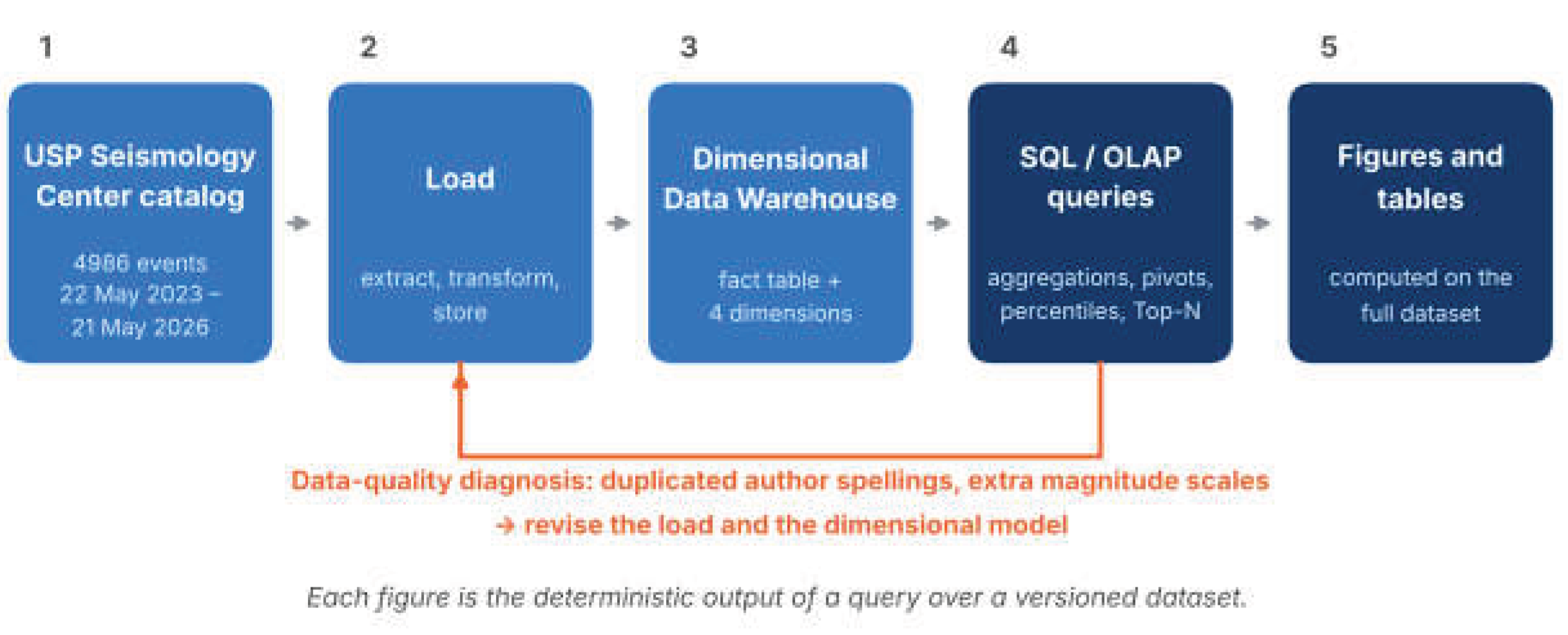
Figure 2.
Dimensional (star) model of the TerremotosUSP Data Warehouse. A fact table stores the event-level measures (magnitude and depth) and is surrounded by four descriptive dimensions: time, location, magnitude scale and author. The attribute lists summarize the dimensions used in the analyses.
Figure 2.
Dimensional (star) model of the TerremotosUSP Data Warehouse. A fact table stores the event-level measures (magnitude and depth) and is surrounded by four descriptive dimensions: time, location, magnitude scale and author. The attribute lists summarize the dimensions used in the analyses.
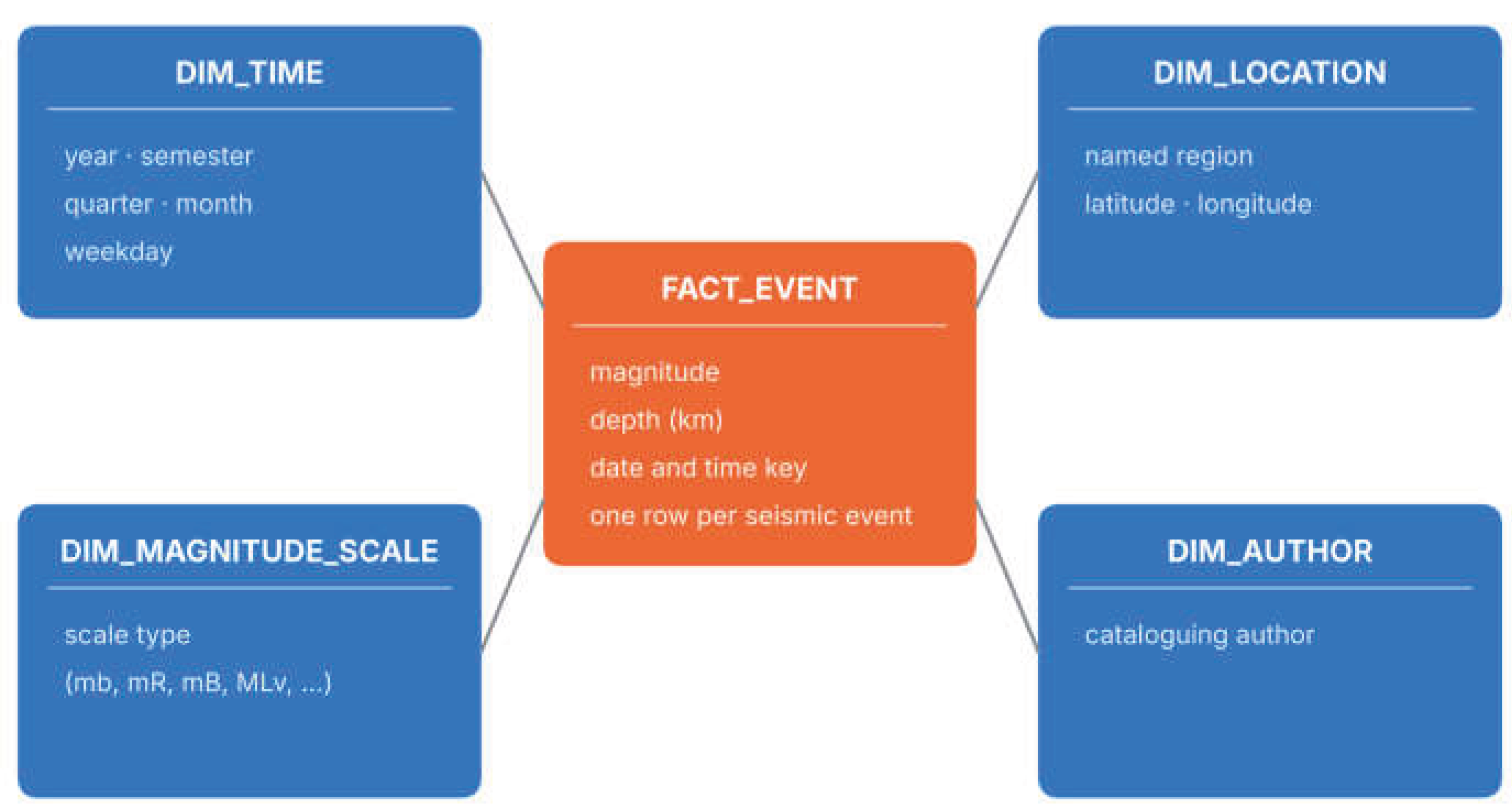
Figure 3.
Magnitude distribution of the 4986 events. (Left) Histogram of magnitudes; the dashed line marks the median (4.81). (Right) Number of events by magnitude class. Source: prepared by the author from the TerremotosUSP Data Warehouse (USP Seismology Center catalog).
Figure 3.
Magnitude distribution of the 4986 events. (Left) Histogram of magnitudes; the dashed line marks the median (4.81). (Right) Number of events by magnitude class. Source: prepared by the author from the TerremotosUSP Data Warehouse (USP Seismology Center catalog).
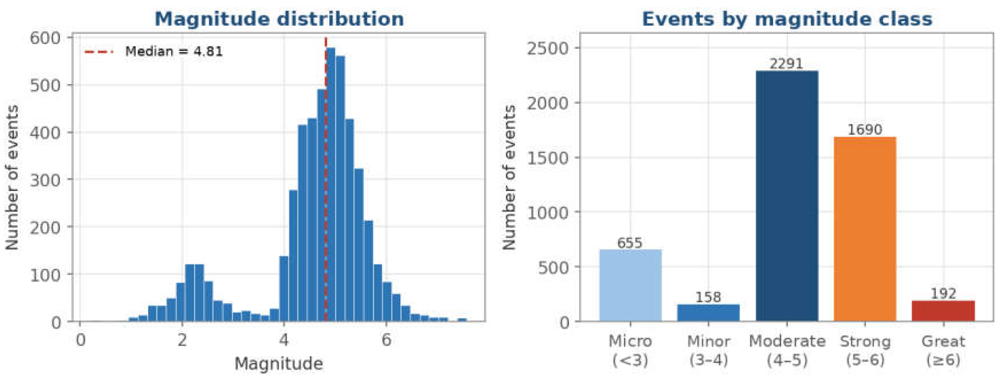
Figure 4.
Focal depth of the events. (Left) Histogram of depth, limited to 350 km for readability. (Right) Number of events by depth range. Source: prepared by the author from the TerremotosUSP Data Warehouse (USP Seismology Center catalog).
Figure 4.
Focal depth of the events. (Left) Histogram of depth, limited to 350 km for readability. (Right) Number of events by depth range. Source: prepared by the author from the TerremotosUSP Data Warehouse (USP Seismology Center catalog).
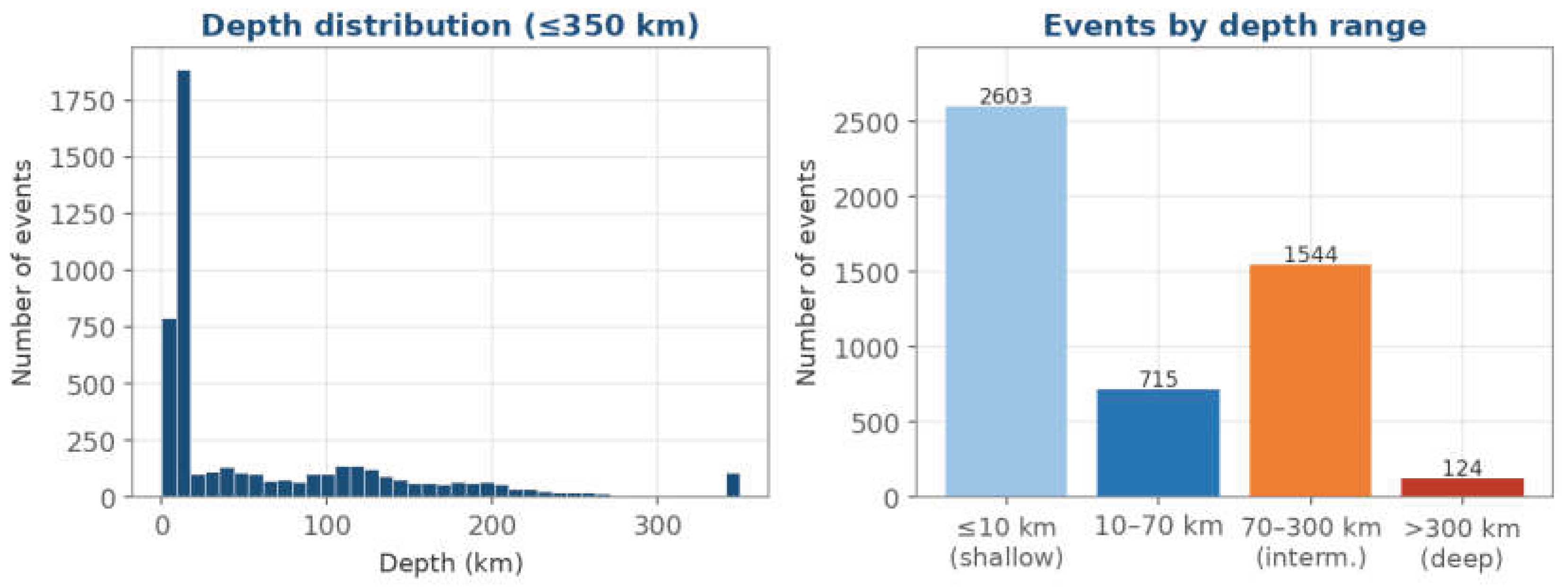
Figure 5.
Temporal evolution of the number of events. (Left) Events per month; the dashed line marks the monthly mean (135). (Right) Cumulative number of events. The first and last months are partial (collection from 22 May 2023 to 21 May 2026). Source: prepared by the author from the TerremotosUSP Data Warehouse (USP Seismology Center catalog).
Figure 5.
Temporal evolution of the number of events. (Left) Events per month; the dashed line marks the monthly mean (135). (Right) Cumulative number of events. The first and last months are partial (collection from 22 May 2023 to 21 May 2026). Source: prepared by the author from the TerremotosUSP Data Warehouse (USP Seismology Center catalog).
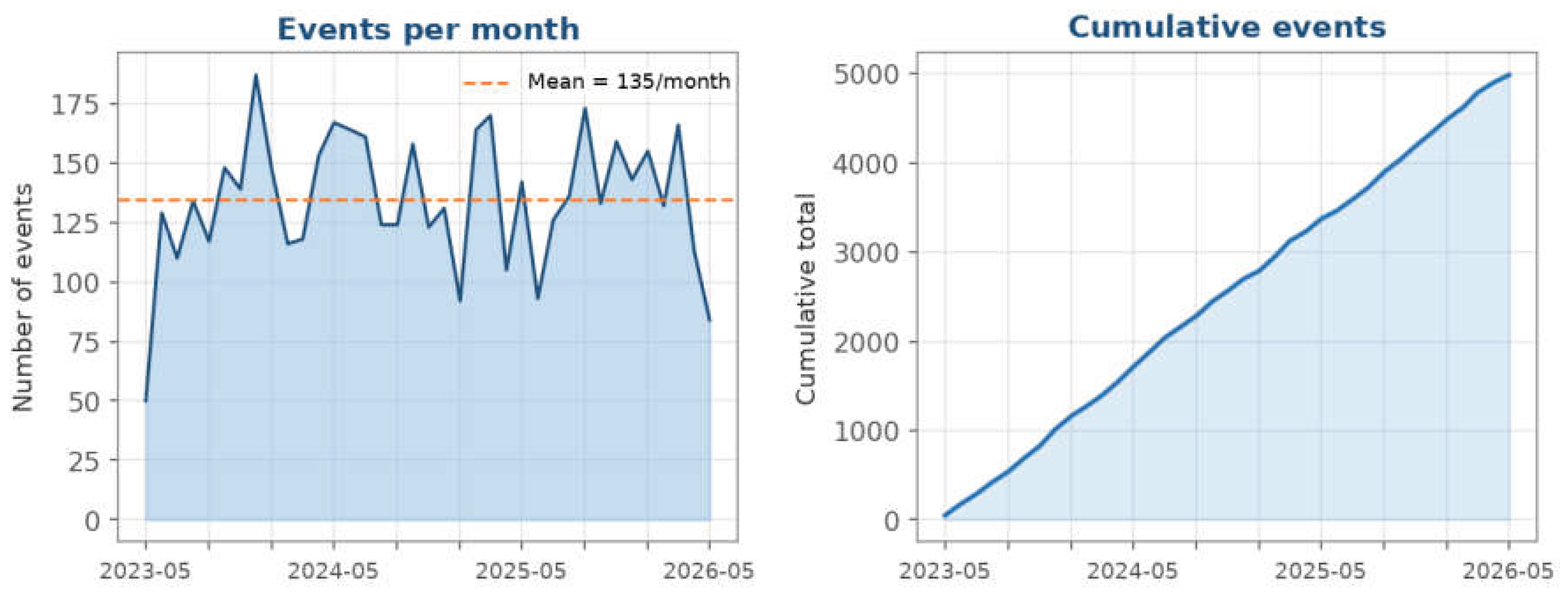
Figure 6.
Global map of epicenters. Color indicates magnitude and symbol size increases with it. Source: prepared by the author from the TerremotosUSP Data Warehouse (USP Seismology Center catalog).
Figure 6.
Global map of epicenters. Color indicates magnitude and symbol size increases with it. Source: prepared by the author from the TerremotosUSP Data Warehouse (USP Seismology Center catalog).
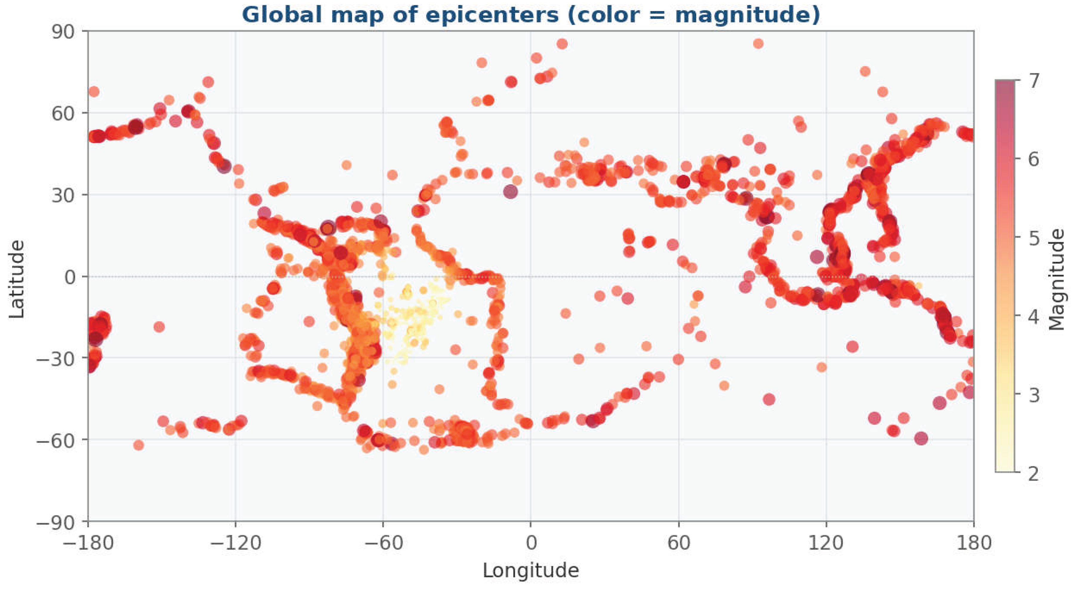
Figure 7.
Joint density of magnitude and depth. Hexagonal binning with a logarithmic color scale. Source: prepared by the author from the TerremotosUSP Data Warehouse (USP Seismology Center catalog).
Figure 7.
Joint density of magnitude and depth. Hexagonal binning with a logarithmic color scale. Source: prepared by the author from the TerremotosUSP Data Warehouse (USP Seismology Center catalog).
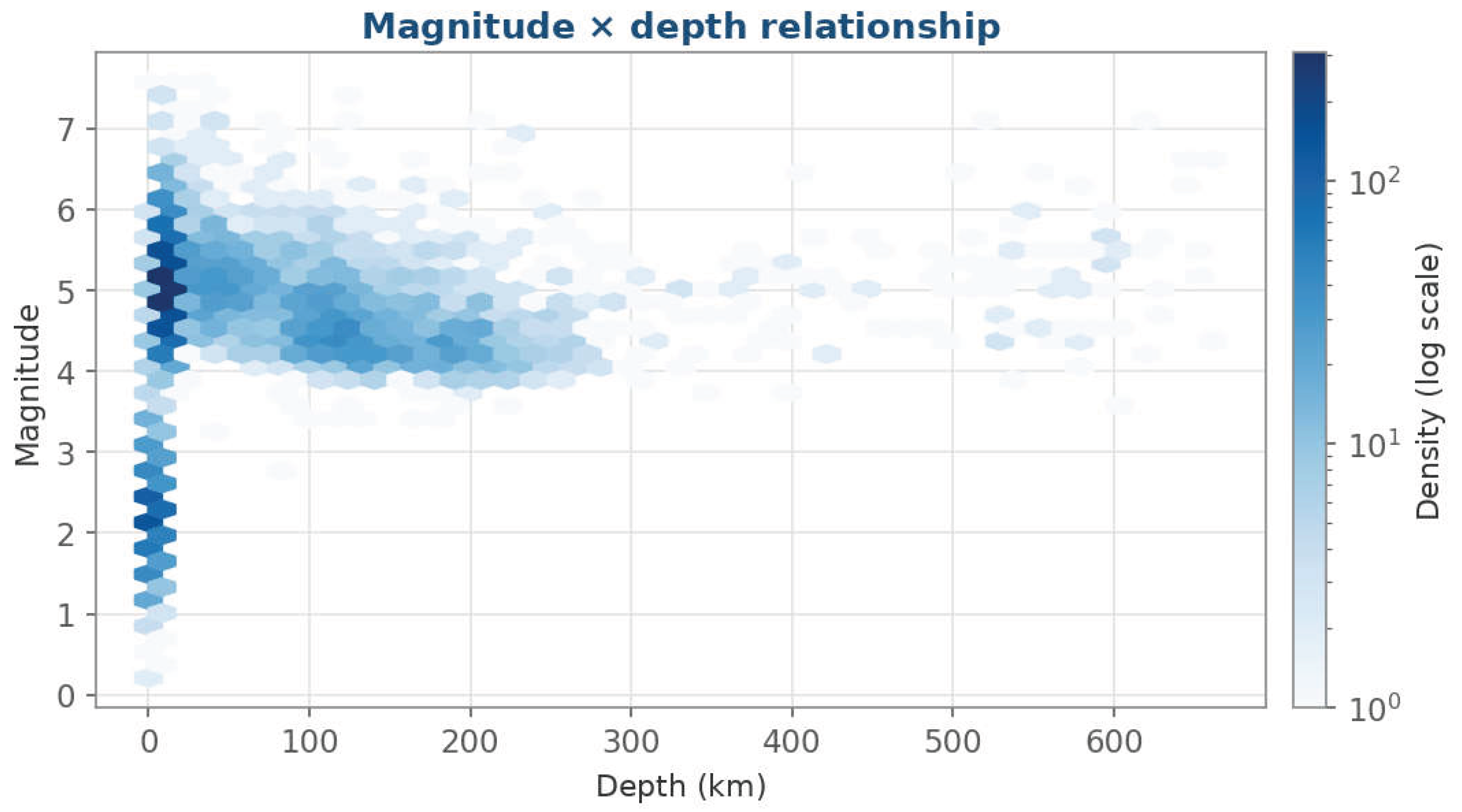
Figure 8.
Q1: Mean magnitude by year and measurement scale. Only the four main scales are shown (mb, mR, mB and MLv); there is no mB bar for 2026. Source: prepared by the author from the TerremotosUSP Data Warehouse (USP Seismology Center catalog).
Figure 8.
Q1: Mean magnitude by year and measurement scale. Only the four main scales are shown (mb, mR, mB and MLv); there is no mB bar for 2026. Source: prepared by the author from the TerremotosUSP Data Warehouse (USP Seismology Center catalog).
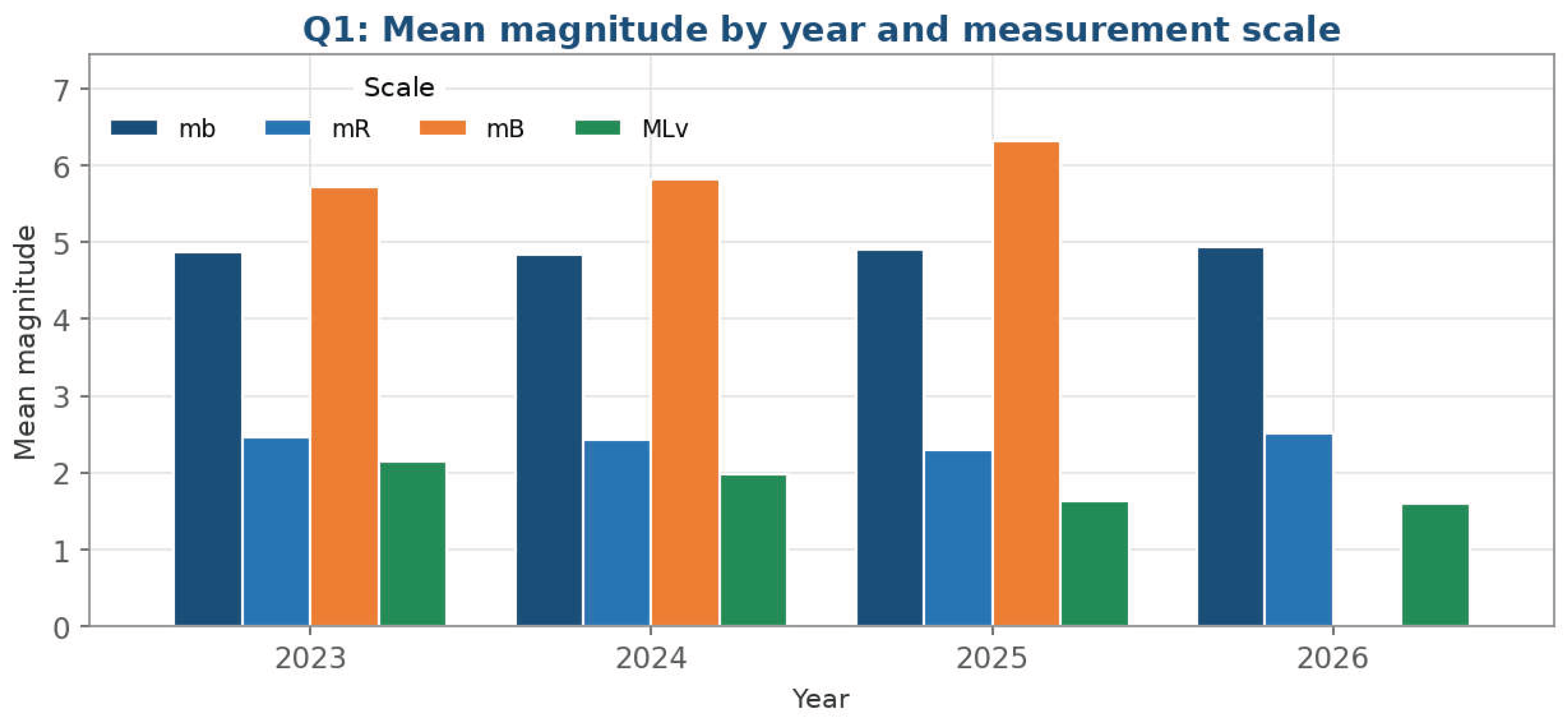
Figure 9.
Q2: Regions with the greatest mean depth. The 12 highest mean depths among regions with at least five events; labels give the mean depth and the number of events (n). Source: prepared by the author from the TerremotosUSP Data Warehouse (USP Seismology Center catalog).
Figure 9.
Q2: Regions with the greatest mean depth. The 12 highest mean depths among regions with at least five events; labels give the mean depth and the number of events (n). Source: prepared by the author from the TerremotosUSP Data Warehouse (USP Seismology Center catalog).
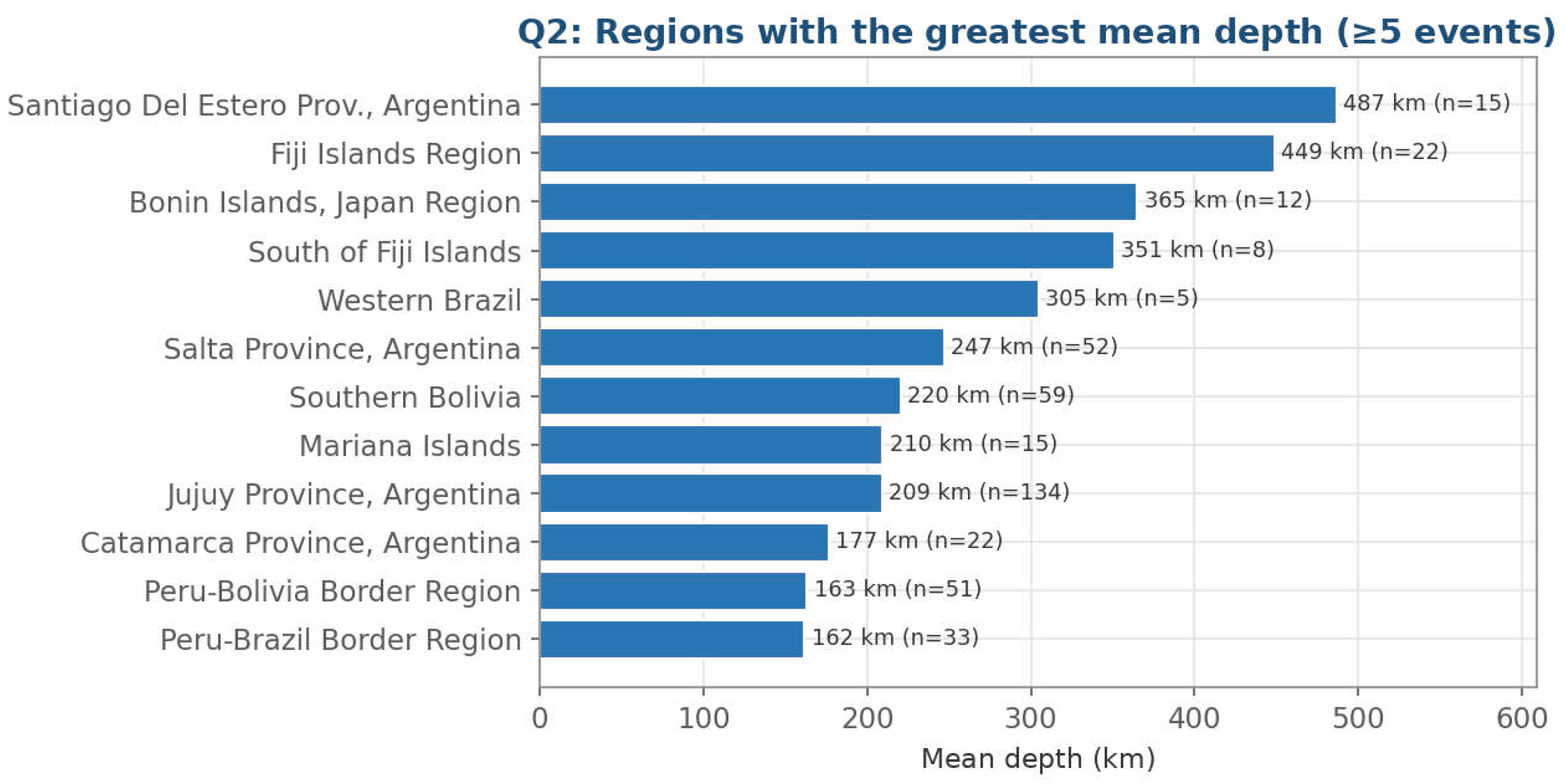
Figure 10.
Q3: Events by weekday and by semester. (Left) Events per weekday; the dashed line marks the mean (712) and weekend days are highlighted. (Right) Events per semester. Source: prepared by the author from the TerremotosUSP Data Warehouse (USP Seismology Center catalog).
Figure 10.
Q3: Events by weekday and by semester. (Left) Events per weekday; the dashed line marks the mean (712) and weekend days are highlighted. (Right) Events per semester. Source: prepared by the author from the TerremotosUSP Data Warehouse (USP Seismology Center catalog).
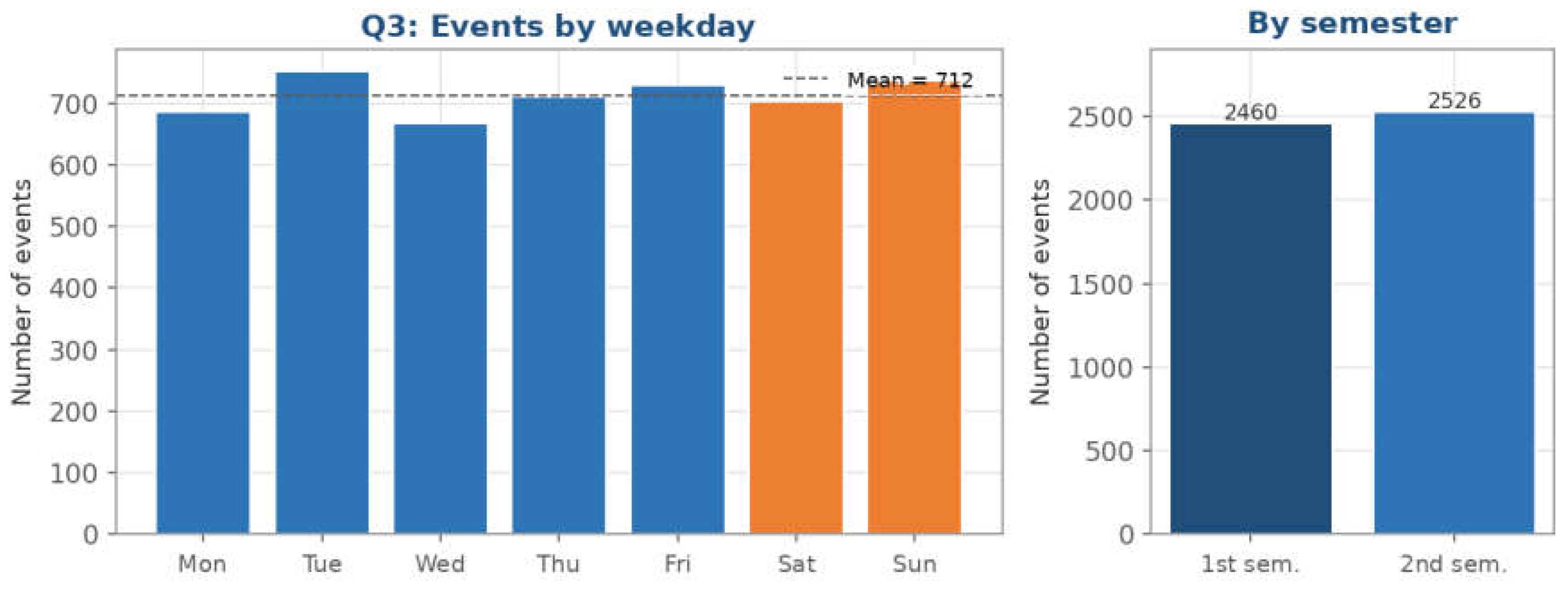
Figure 11.
Q4: Events cataloged by author and year. The spellings J.Alexandre and JAlexandre, which refer to the same author, were merged. Bar labels give the total per author. Source: prepared by the author from the TerremotosUSP Data Warehouse (USP Seismology Center catalog).
Figure 11.
Q4: Events cataloged by author and year. The spellings J.Alexandre and JAlexandre, which refer to the same author, were merged. Bar labels give the total per author. Source: prepared by the author from the TerremotosUSP Data Warehouse (USP Seismology Center catalog).
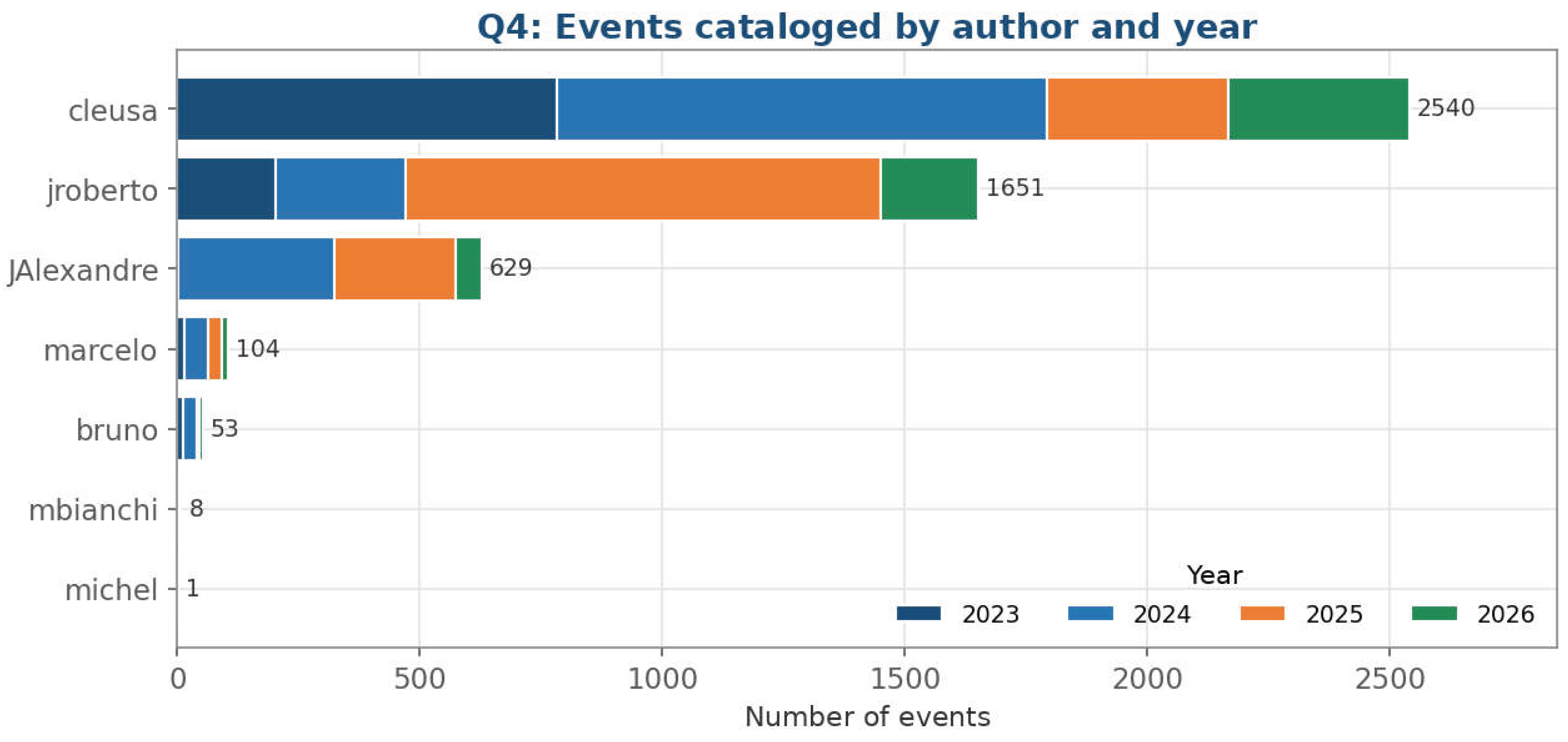
Figure 12.
Pivot: Number of events by year and quarter. Values correspond to Table 3; blank cells are quarters outside the observation window. Source: prepared by the author from the TerremotosUSP Data Warehouse (USP Seismology Center catalog).
Figure 12.
Pivot: Number of events by year and quarter. Values correspond to Table 3; blank cells are quarters outside the observation window. Source: prepared by the author from the TerremotosUSP Data Warehouse (USP Seismology Center catalog).
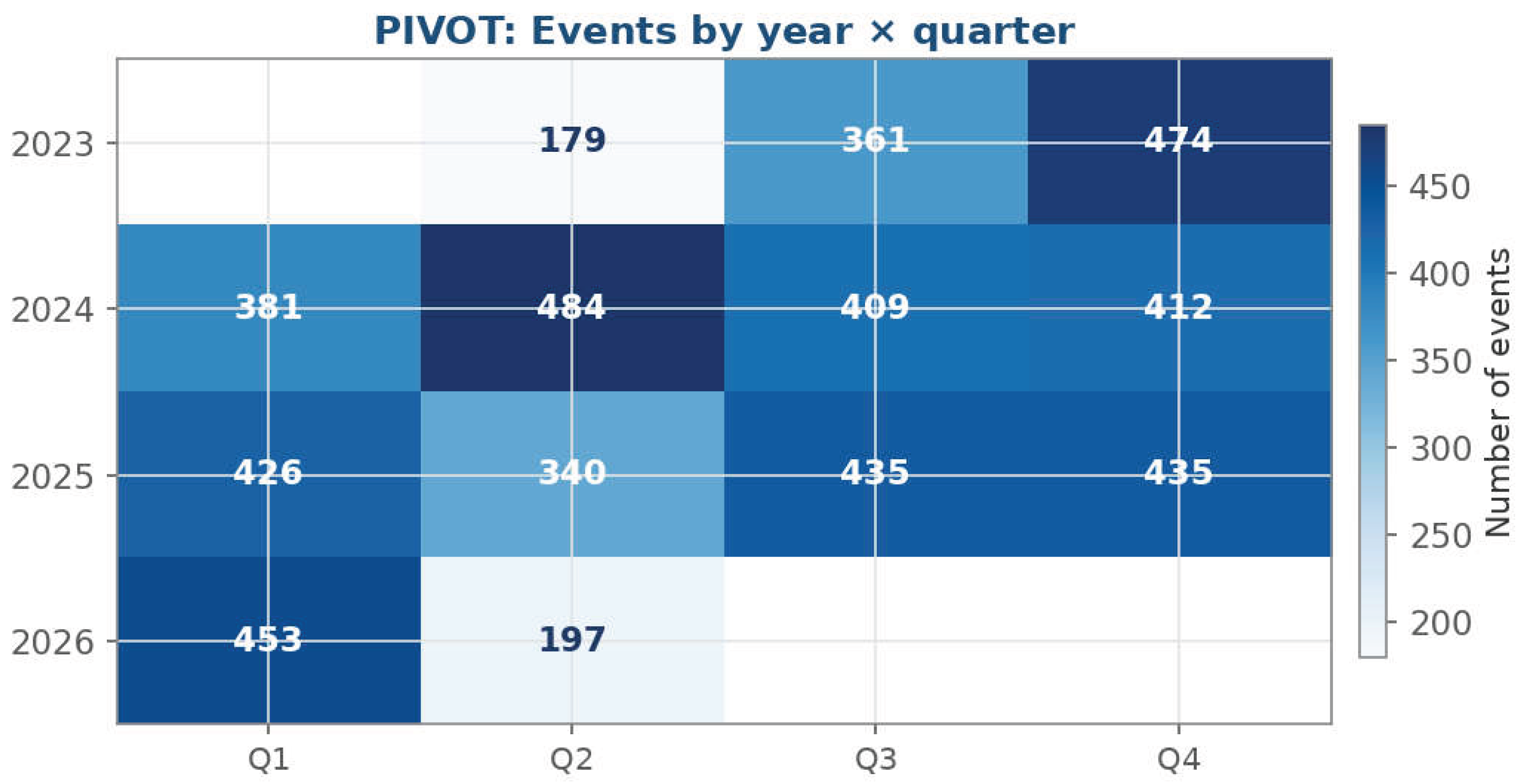
Figure 13.
Magnitude percentiles by year. P10, median (P50) and P90 of the magnitude computed with PERCENTILE_CONT. Source: prepared by the author from the TerremotosUSP Data Warehouse (USP Seismology Center catalog).
Figure 13.
Magnitude percentiles by year. P10, median (P50) and P90 of the magnitude computed with PERCENTILE_CONT. Source: prepared by the author from the TerremotosUSP Data Warehouse (USP Seismology Center catalog).
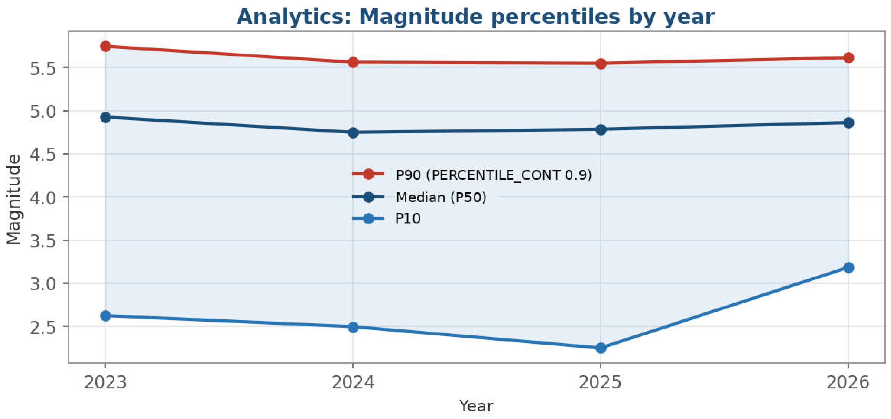
Figure 14.
Brazil and international events. (Left) Share of events located in Brazil and abroad. (Right) Magnitude distribution by origin (box plots). Source: prepared by the author from the TerremotosUSP Data Warehouse (USP Seismology Center catalog).
Figure 14.
Brazil and international events. (Left) Share of events located in Brazil and abroad. (Right) Magnitude distribution by origin (box plots). Source: prepared by the author from the TerremotosUSP Data Warehouse (USP Seismology Center catalog).
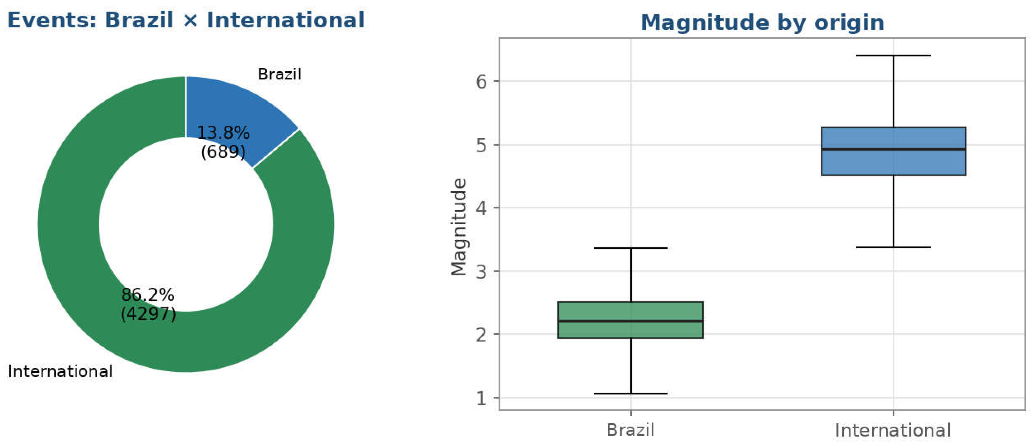
Figure 15.
Magnitude scales and annual magnitude distribution. (Left) Number of events by magnitude scale: eight scales were observed against six defined in the dimensional model. (Right) Magnitude by year (box plots; red lines mark the medians). Source: prepared by the author from the TerremotosUSP Data Warehouse (USP Seismology Center catalog).
Figure 15.
Magnitude scales and annual magnitude distribution. (Left) Number of events by magnitude scale: eight scales were observed against six defined in the dimensional model. (Right) Magnitude by year (box plots; red lines mark the medians). Source: prepared by the author from the TerremotosUSP Data Warehouse (USP Seismology Center catalog).
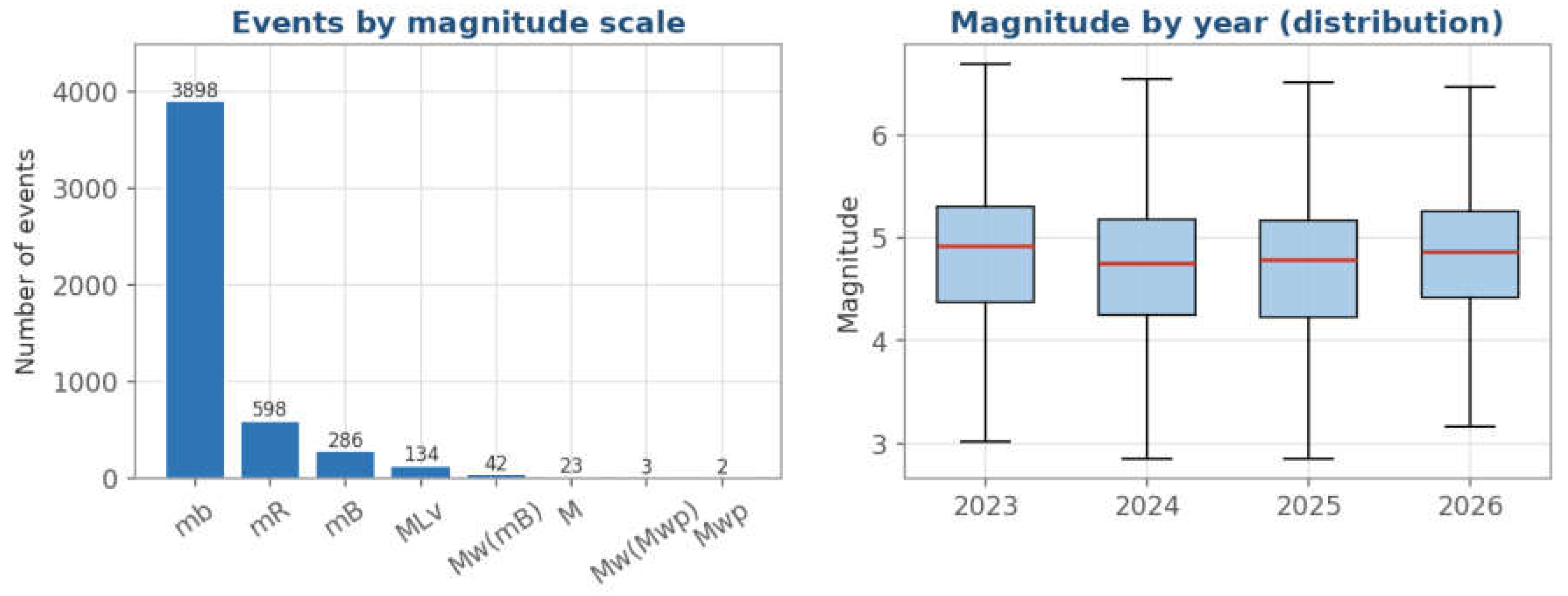

Table 1.
Key figures of the dataset analyzed.
| Indicator | Value |
|---|---|
| Total events | 4986 |
| Period covered | 22 May 2023 to 21 May 2026 |
| Median / maximum magnitude | 4.81 / 7.58 |
| Shallow events (≤10 km) | 52.2% |
| Events in Brazil / international | 689 / 4297 |
| Most active region | Chile–Bolivia border region (263 events) |
| Distinct magnitude scales | 8 |
Source: prepared by the author from the TerremotosUSP Data Warehouse (USP Seismology Center).
Table 2.
Catalog of the analytical (OLAP) queries and where their results are reported.
| Query | Analytical question | OLAP operation / SQL construct | Reported in |
|---|---|---|---|
| Q1 | Mean magnitude by year and magnitude scale | Aggregation (AVG) with GROUP BY; control by the scale dimension | Section 4.2.1 |
| Q2 | Regions with the greatest mean depth (at least five events) | Aggregation (AVG); HAVING COUNT(*) ≥ 5; ranking | Section 4.2.2 |
| Q3 | Event frequency by weekday and semester | Aggregation (COUNT) with GROUP BY over time attributes | Section 4.2.3 |
| Q4 | Production by author and year | Aggregation (COUNT); grouping by the author dimension | Section 4.2.4 |
| Pivot | Events by year and quarter | Contingency table (pivoting) | Section 4.2.5 |
| Percentiles | Magnitude distribution by year (P10, P50, P90) | PERCENTILE_CONT as an ordered-set / window function | Section 4.2.6 |
| Top-N | Ten largest events of the period | Ranking (ORDER BY … DESC) with row limiting | Section 4.2.7 |
Source: prepared by the author from the documentation of the TerremotosUSP project.
Table 3.
Number of events by year and quarter (– = no data in the observation window).
| Year | Q1 | Q2 | Q3 | Q4 | Total |
|---|---|---|---|---|---|
| 2023 | – | 179 | 361 | 474 | 1014 |
| 2024 | 381 | 484 | 409 | 412 | 1686 |
| 2025 | 426 | 340 | 435 | 435 | 1636 |
| 2026 | 453 | 197 | – | – | 650 |
| Total | 1260 | 1200 | 1205 | 1321 | 4986 |
Source: prepared by the author from the TerremotosUSP Data Warehouse. Row and column totals were computed from the table values.
Table 4.
The ten largest earthquakes in the catalog (22 May 2023–21 May 2026).
| Rank | Region | Date | Magnitude |
|---|---|---|---|
| 1 | North of Honduras | 8 February 2025 | 7.58 |
| 2 | Near East Coast of Kamchatka | 18 September 2025 | 7.51 |
| 3 | Mindanao, Philippines | 2 December 2023 | 7.50 |
| 4 | Myanmar | 28 March 2025 | 7.49 |
| 5 | Near West Coast of Honshu, Japan | 1 January 2024 | 7.46 |
| 6 | Taiwan | 2 April 2024 | 7.44 |
| 7 | Chile–Bolivia Border Region | 19 July 2024 | 7.40 |
| 8 | Vanuatu Islands | 17 December 2024 | 7.39 |
| 9 | Off East Coast of Honshu, Japan | 20 April 2026 | 7.26 |
| 10 | Near Coast of Peru | 28 June 2024 | 7.22 |
Source: prepared by the author from the TerremotosUSP Data Warehouse.
Table 5.
Data-quality issues revealed by the analysis and suggested remediation.
| Issue | Detected in | Evidence | Suggested remediation |
|---|---|---|---|
| Duplicated author spelling | Q4 (Section 4.2.4) | J.Alexandre and JAlexandre refer to the same author | Standardize names when the authorship dimension is loaded |
| Magnitude scales beyond the model | Scale count (Section 4.3.2) | Eight scales observed against six defined; Mw(Mwp) and Mwp were not foreseen | Revise the loading of the magnitude-type dimension |
| Zero depth as indeterminacy | Depth analysis (Section 4.1.2) | Many shallow events have depth equal to zero, flagged by the Center | Interpret zero as a marker of indeterminacy, not as a measurement |
| Partial observation windows | Temporal series (Section 4.1.3 and Section 4.2.5) | 2023 and 2026 are incomplete (22 May 2023 to 21 May 2026) | Read annual aggregates against their observation windows |
Source: prepared by the author from the results ofSection 4.
Table 6.
Methodological properties conferred by query-mediated visualization and evidence from the case study.
Table 6.
Methodological properties conferred by query-mediated visualization and evidence from the case study.
| Property | Operational meaning | Evidence from the case | Related literature |
|---|---|---|---|
| Reproducibility | Same dataset and same query yield the same figure | Each figure is the deterministic output of a query over a versioned dataset | [1,2] |
| Traceability | Each figure can be followed back to its query and data | The routine that queries the Data Warehouse also generates the figure | [11,12,14,15] |
| Computational accuracy | Values are computed over the full dataset with the declared construct | PERCENTILE_CONT for P10–P90; minimum-events filter in Q2; contingency table | [9] |
| Scalability | Analytical logic is invariant to data volume | Same queries expected to hold for larger catalogs (not benchmarked here) | [6,7] |
| Diagnostic capacity | Aggregation exposes inconsistencies in the data | Duplicated author spelling; eight scales against six; partial windows | [10] |
Source: prepared by the author.
Disclaimer/Publisher’s Note: The statements, opinions and data contained in all publications are solely those of the individual author(s) and contributor(s) and not of MDPI and/or the editor(s). MDPI and/or the editor(s) disclaim responsibility for any injury to people or property resulting from any ideas, methods, instructions or products referred to in the content. |
© 2026 by the authors. Licensee MDPI, Basel, Switzerland. This article is an open access article distributed under the terms and conditions of the Creative Commons Attribution (CC BY) license (http://creativecommons.org/licenses/by/4.0/).
Copyright: This open access article is published under a Creative Commons CC BY 4.0 license, which permit the free download, distribution, and reuse, provided that the author and preprint are cited in any reuse.