

Submitted:
14 November 2026
Posted:
16 November 2026
You are already at the latest version
Abstract
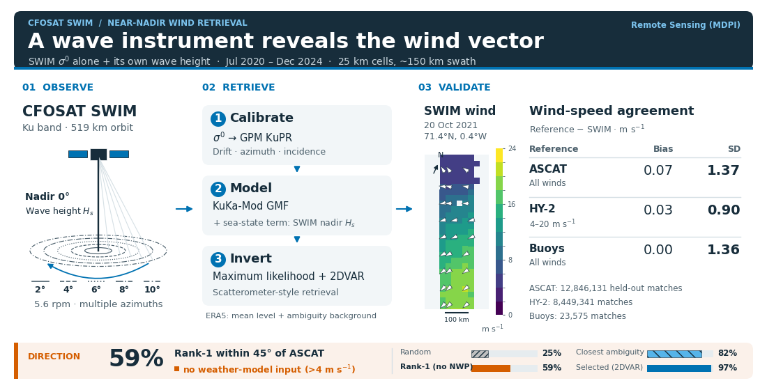
The Surface Waves Investigation and Monitoring instrument (SWIM) on the China–France Oceanography Satellite (CFOSAT) is a Ku-band rotating radar with nadir and five off-nadir beams (2–10°). This study retrieves the wind vector from SWIM's normalized radar cross section (σ⁰) alone and assesses its own direction information. Recalibrated to the Global Precipitation Measurement Ku-band radar, σ⁰ is inverted with a model of stress-equivalent wind and wave height, ERA5 setting the mean level and ambiguity-removal background. Against the Advanced Scatterometer (ASCAT), over 12 million held-out matches of the July 2020–December 2024 record (25 km grid) give, at all winds, a speed bias of 0.07 m s⁻¹ (ASCAT − SWIM) and a standard deviation of 1.37 m s⁻¹; triple collocation of matches within 30 min gives SWIM about twice the ASCAT error. Bias and standard deviation are 0.03 and 0.90 m s⁻¹ against the Haiyang-2 (HY-2) scatterometers at 4–20 m s⁻¹, and 0.00 and 1.36 m s⁻¹ against buoys at all winds. In 2 m s⁻¹ bins of mean wind from 4 to 22 m s⁻¹, the ASCAT bias stays within 0.26 m s⁻¹. With the wave-height term, the buoy wave-height slope is similar to those of ERA5 and HY-2; a residual slope remains against ASCAT. Above 4 m s⁻¹, without weather-model input, the rank-1 direction lies within 45° of ASCAT in 59% of cells.
Keywords:
CFOSAT
; SWIM
; near-nadir radar
; Ku-band
; wind retrieval
; calibration
; scat- 18 terometer
; stress-equivalent wind
; sea state
; triple collocation
1. Introduction
Satellite radars measure the ocean surface wind through the roughness of the short waves, which sets the normalized radar cross section of the sea surface, . Scatterometers observe at moderate incidence angles, roughly 20–, where the backscatter is resonant (Bragg) scattering by centimetre waves and increases with wind speed. Their rotating or multiple fixed antennas view each wind cell from several azimuths and retrieve the wind vector [1]. Radar altimeters observe at nadir, where the return is dominated by specular reflection from surface facets and decreases with wind as the surface slopes broaden. They provide wind speed along the ground track only [2,3,4]. Between the two, at near-nadir incidence, the return is still dominated by specular reflection up to about 10–, beyond which resonant scattering gradually takes over [5]. Spaceborne observations there came mainly from the precipitation radars of the Tropical Rainfall Measuring Mission and of the Global Precipitation Measurement (GPM) mission [6,7,8], which view each cell from a single azimuth.
The Surface Waves Investigation and Monitoring instrument (SWIM) on the China–France Oceanography Satellite (CFOSAT) is the first spaceborne wave scatterometer [9,10]. Designed to measure the directional spectrum of ocean waves, it illuminates the sea at nadir () and at 2, 4, 6, 8 and while its antenna turns, so that most wind cells of its swath are seen by the off-nadir beams at several incidences and many azimuths, and the nadir beam measures the significant wave height along the track. This is the sampling that a wind-vector retrieval needs: the incidence dependence constrains the wind speed and the weak azimuthal modulation the wind direction. CFOSAT also carries a rotating fan-beam wind scatterometer, SCAT [11], so wind from SWIM is both a test of near-nadir wind retrieval and a second wind measurement on the same platform, independent of the SCAT .
Wind information from SWIM has so far been used in four ways. The nadir beam provides an altimeter-type wind speed along the ground track [10,12]. The off-nadir has been inverted for wind speed alone, after an ocean recalibration against numerical weather prediction (NWP) winds and with a Ku-band low-incidence model function from precipitation-radar data, with errors growing above incidence [13]. Wind speed in tropical cyclones has also been estimated from the SWIM wave spectra [14]. Finally, SWIM measurements have been used to constrain the wind retrieval of the CFOSAT scatterometer [15] or in a joint SWIM–SCAT inversion [16]. At near-nadir incidence, the dependence of Ku- and Ka-band on wind direction has been characterized from GPM [8,17], and the wind speed, including gale winds, has been retrieved from the GPM Ku-band swath [18,19], but the azimuthal modulation has not been inverted for the wind direction.
SWIM was designed as a wave instrument, not as a scatterometer. Its wave spectra rest on the relative modulation of along the look direction, so the absolute level of , its stability in time and the consistency between beams were not monitored systematically, as they are for scatterometers. A SWIM-only retrieval of the wind vector therefore has four requirements. The of each beam must be calibrated in time and in absolute level, because drifts and beam-to-beam differences matter more for wind than for wave retrieval. A geophysical model function (GMF) for the near-nadir range, valid in azimuth and referenced to the same wind definition as scatterometers, was lacking. Near nadir, also depends on the sea state, through the slopes of the longer waves that tilt the scattering facets [20,21], and a model of wind alone turns this dependence into wind errors. And the wind direction signal at near-nadir incidence is weak, so the retrieval must quantify how much direction information SWIM carries by itself. The companion papers derive and fit the GMF from the dual-frequency GPM radar [5,22]. The present paper addresses the other three requirements, to assess whether SWIM alone can provide useful wind vectors and how much direction information it contributes. It calibrates the five SWIM beams to the GPM Ku-band radar, adds to the GMF a sea-state term driven by the wave height that SWIM measures itself, and inverts the beams for the wind vector with scatterometer methods. The record from July 2020 to December 2024 is then validated against the Advanced Scatterometer (ASCAT), the Haiyang-2 (HY-2) scatterometers and moored buoys; the validation separates the direction information of SWIM from that of the NWP background and leads to limits for use of the product.
2. SWIM Instrument and Data
2.1. The SWIM Instrument
CFOSAT, launched on 29 October 2018 into a 519 km polar orbit with a 13-day repeat cycle, carries the rotating fan-beam scatterometer SCAT and the wave scatterometer SWIM [9,10]. SWIM is a Ku-band ( GHz) real-aperture radar that illuminates the sea successively at 0, 2, 4, 6, 8 and incidence while its antenna rotates at rpm. Each beam has a footprint of about 18 km, and the beam reaches about 90 km on either side of the track, so that every off-nadir beam views the sea over the full of azimuth within a 180 km swath (Figure 1). The off-nadir beams are named by their incidence, beam 2 to beam 10.
In the 0– range the return is dominated by specular reflection: is set by the slope statistics of the short waves and decreases with wind speed. The sensitivity to wind is largest at the inner beams and nearly vanishes at [22]; the azimuthal modulation, which carries the wind direction, is weak and grows with incidence.
2.2. Data
SWIM. We use the SWIM Level-2S (L2S) product of the IFREMER Wind and Wave Operational Center (IWWOC) [23], which gives the of each off-nadir beam along the range of every antenna look, with position, incidence and azimuth. Each averages over the 18 km footprint across the look direction [10]. The product also gives the significant wave height measured by the nadir beam along the track. We use versions v2.0 and v2.1 from 2020-07-01 to 2024-12-08, in the conventional mode only (nadir and all five off-nadir beams): half-orbits. Excluded are the commissioning period (2019-04 to 2020-06, when the instrument level was unstable) and the reduced-beam modes (Table 1), including the two-beam mode used since 2024-12-08.
Reference winds. All winds in this study are stress-equivalent 10 m winds [24], that is, neutral 10 m winds that would produce the observed surface stress at a standard air density; this is the definition used by scatterometer products. The reference is the ASCAT wind product of the Royal Netherlands Meteorological Institute (KNMI), distributed by the Ocean and Sea Ice Satellite Application Facility (OSI SAF), on Metop-B and Metop-C (12.5 km coastal product) [25,26], available over the whole record from two instruments with well-characterized errors. The KNMI winds of the scatterometers on HY-2B, -2C and -2D (25 km product) [27,28], available from July 2020, November 2020 and November 2023, provide a second reference from instruments on separate platforms. The background wind is the fifth-generation reanalysis (ERA5) of the European Centre for Medium-Range Weather Forecasts (ECMWF) [29], converted to the same definition; ERA5 also provides sea-surface temperature, water vapour, cloud liquid water, sea ice and the significant wave height.
Buoys. Moored buoys of the Copernicus Marine Service in situ network [30] provide an in situ reference over the whole record. Only buoys at least 25 km offshore are used. Their wind, averaged over min, is converted to the stress-equivalent 10 m wind with a neutral logarithmic profile and the ERA5 air density, without a stability correction. Where the buoy measures waves, its significant wave height is used. To place the SWIM errors among classical scatterometers, the same buoys, with the same processing, are also matched with ASCAT, HY-2 and the CFOSAT scatterometer [31] at the pass time of each instrument.
3. Methods
3.1. Calibration of SWIM
The level of the L2S is neither stable in time nor consistent between beams to the accuracy a wind retrieval needs: on beam 2 a level error of dB corresponds to about m of wind. The calibration brings every beam to the GPM KuPR scale in three steps (Figure 2).
Drift. The daily level of each beam is tracked on a narrow, stable subset of the data (moderate winds, fixed geometry) and referenced to the period 2021-01 to 2022-06. It reveals the rising level of the commissioning period, a flat level in 2021–2022, and an instantaneous, beam-dependent gain step of up to dB at the end of an instrument outage on 2022-08-17 (Figure 2a).
Azimuth. A small modulation with the look azimuth in the satellite frame, different for each beam and largest on beam 2 ( dB), is consistent with a slight mispointing. This instrumental modulation is removed before the wind-relative modulation is used (Figure 2c).
Incidence. Each beam carries its own effective gain profile, so that the beams disagree where their incidences overlap. Collocations with GPM KuPR (10 km, 30 min, 2021–2023) give a per-beam, incidence-dependent offset, from dB at beam 2 to dB at beam 10 (Figure 2b); after correction, the residual SWIMKuPR offset has a root-mean-square value of to dB in each year. These are direct comparisons, involving no model; because the GMF is fitted on KuPR , this step also puts SWIM on the scale of the GMF.
3.2. Geophysical Model Function
The forward model is KuKa-Mod, a near-nadir Ku/Ka model function derived and fitted on GPM in the companion papers [5,22]; its parameters, look-up tables and reference evaluator are archived on Zenodo [34]. It describes as a function of incidence , wind speed U and the angle between the antenna look direction and the direction towards which the wind blows ( looking downwind),
where the isotropic part follows from the Kirchhoff scattering of a sea surface whose short-wave slope statistics depend on wind, and the harmonics and give the up/downwind and up/crosswind modulation; their form is set by SWIM and their amplitudes by GPM KuPR [22]. For this work the model is referenced to stress-equivalent wind, using GPM KuPR collocated with scatterometer winds. Above 4 m its level is adjusted to SWIM by an empirical correction, a smooth function of wind speed and incidence, fitted to the SWIM of the odd months of 2021–2024 [22]. In each incidence bin the distribution of the SWIM is matched to the distribution that the model predicts from the ASCAT winds, with an allowance for the random errors of both. Averaging in bins of the reference wind would instead select, at high wind, the matches where the reference reads high, and make the model too bright there. HY-2, whose matches at reference winds above 15 m are taken from all its passes, sets the shape of the correction beyond the wind range covered by ASCAT; beyond the data it is held constant, and the model extends to 50 m . This correction is a calibration of the model level for SWIM, not part of the physical model, and is released with KuKa-Mod as its SWIM high-wind table [34].
Sea state. The longer waves tilt the short-wave facets and add to the slope variance that the radar sees, so that at a given wind near nadir depends on the sea state [20,21,22]. In KuKa-Mod the slope statistics enter through the lag-dependent slope variance of the surface, a logarithmic function of the lag whose additive coefficient sets its level [5]. The response is carried by the long-wave slope variance; KuKa-Mod predicts its incidence dependence but leaves its size unfitted, because the measured size depends on the reference wind [22]. Here , which SWIM measures, serves as its proxy: the sea-state term adds to a an increment proportional to the departure of the significant wave height from its mean at that wind,
with U in m , and a small level term of c dB per metre of the same departure. The incidence dependence of the term follows from the model: it darkens the inner beams in a high sea, weakens with incidence and changes sign near , as observed on SWIM and GPM [22]. The three constants, , and dB , are fitted against the HY-2 winds of the odd months in classes of ERA5 wind rather than of HY-2 wind, which limits the effect of the reference-wind error on the fit. At the term vanishes and the mean level of the model is unchanged. The model is used as a four-dimensional table in incidence, wind speed, relative azimuth and .
3.3. Wind Retrieval
The winds are retrieved with the General Utility Scatterometry Tool (GUST), whose inversion and ambiguity removal follow the KNMI scatterometer processors [35,36,37]. Each half-orbit goes through the steps of Figure 3.
Grid and views. Wind vector cells (WVCs) are defined on a 25 km grid along the nadir track, eight cells across the swath, numbered 0 to 7; cells 1 to 6 form the inner swath, and the edge cells 0 and 7 are reached only by beams 8 and 10. The calibrated L2S segments that fall near a WVC are grouped by beam and antenna look into views. A usable WVC of the inner swath has a median of 52 views from all five beams and many azimuths. The views are collected within about 18 km of the WVC centre and each footprint is 18 km wide, so the wind is supported by an area about 50 km across, which sets the effective resolution.
Sea-state input. The of each WVC is that of the SWIM nadir beam, from the same half-orbit; ERA5 is used where it is missing.
Corrections. Before inversion, is corrected for the two-way attenuation by water vapour and cloud liquid water, computed from ERA5 with the models of the International Telecommunication Union Radiocommunication Sector (ITU-R) [38,39]. It reaches about dB in moist tropical air and is not applied in the L2S product. A second correction accounts for the dependence of the sea-surface reflectivity on temperature [40]. A final ocean calibration against the GMF at the ERA5 wind, per beam and cross-track position, as in scatterometry [41], corrects the remaining level difference of a few tenths of a decibel and ties the mean SWIM level to ERA5.
Inversion and ambiguity removal. For each WVC, a maximum-likelihood search over wind speed and direction compares the views with the GMF. Its noise model, estimated against ASCAT winds, accounts for the speckle noise of each view and for the errors shared by the views of a beam. The inversion gives the likelihood of every wind direction; its up to four local maxima are the ambiguities, and the most likely one, the rank-1 solution, uses no NWP information. A two-dimensional variational analysis (2DVAR) combines the full direction likelihood of each WVC (multiple-solution scheme) with the ERA5 background wind, and the selected wind is the solution closest to the analysis [35,36]. It need not be one of the four ambiguities.
Quality control. WVCs over land or ice, with too few or inconsistent views, or rejected by the 2DVAR quality control are flagged. Winds below 3 m and above 18 m carry a warning flag; the recommended range nevertheless begins at 4 m (Table 4).
Reprocessing. The record 2020-07-01 to 2024-12-08 was reprocessed on the IFREMER Datarmor computing centre into a level-2 product in the format of the KNMI scatterometer winds (working name SWI_WND, version 2.3). Of the eligible half-orbits, were processed; the others, mostly in late 2023 and early 2024, are missing from the input or failed in processing and will be added in the next reprocessing. The output covers all 54 months.
3.4. Validation
Reference. Each usable SWIM WVC is matched with the ASCAT cells within km and 2 h, whose wind vectors are averaged; the median time separation is min. The wind scale of the GMF comes from GPM observations matched with scatterometer winds, ASCAT among them, so SWIM and ASCAT share that scale. SWIM matches with the scatterometers enter the empirical level correction and the sea-state term of the GMF (odd months of 2021–2024, ASCAT and HY-2) and the SWIM noise model (January and July 2021). Except in the monthly time series, the scatterometer statistics exclude these 24 fit months and use the held-out months: July to December 2020 and the even months of 2021–2024. ERA5 is not independent of SWIM: it is the 2DVAR background and sets the mean level through the ocean calibration, and it is shown for context.
CFOSAT scatterometer. SCAT, on the same platform, gives simultaneous winds, but it is not used as the validation reference. Its antenna stopped rotating on 1 December 2022, after which no wind vectors can be retrieved [31,42], so it covers only the first 29 of the 54 months and none of the later part of the record, where the stability of SWIM has to be shown. The SWIM swath also lies in the nadir part of the SCAT swath, where the azimuth diversity is limited and the directions are less accurate than in the outer part of the SCAT swath [41]. ASCAT spans the whole record with two instruments independent of CFOSAT and is the primary reference.
Second reference. The HY-2 scatterometers are matched to SWIM in the same way, within km, and pass closer in time to CFOSAT (median 44 min); they test whether the results depend on the choice of reference. A random 20 % of their matches is used. Each buoy is matched with the nearest usable SWIM WVC within 25 km; the buoys enter no fit, so all months are used.
Statistics. SWIM is plotted on the horizontal axis and the reference on the vertical axis, and differences are reference minus SWIM: a negative bias means that SWIM reads high. Speed is assessed by bias, standard deviation (SD), root-mean-square difference (RMSD) and correlation, and the wind vector by the SDs of the zonal and meridional components. Residual statistics are binned by the mean of the two winds, because binning by either wind alone selects the errors of that wind and creates an artificial dependence on speed [43]. Speed errors are estimated by triple collocation of SWIM, ASCAT and ERA5 [43,44] on the matches within 30 min, on the ASCAT scale. The method assumes uncorrelated errors and a common linear relation to the true wind; the shared processing of SWIM and ERA5 and their coarser resolution than ASCAT may violate it, so the estimates are indicative. It is not applied to the components, because the 2DVAR draws the selected SWIM direction towards the ERA5 background and correlates their component errors. Direction is assessed for mean winds above 4 m (directions towards which the wind blows, differences wrapped to ) by the fraction of cells within of ASCAT, for the rank-1 solution, for the closest of the ambiguities, and for the selected solution. The rank-1 solution uses no NWP direction information, but its sample, like all others, is the set of WVCs that pass quality control.
Sea state. The dependence on sea state is measured by the slope of the speed difference on for mean winds of 4–20 m , fitted with a separate offset in each 2 m class of mean wind, which absorbs the mean difference between wind classes. is the buoy wave height for the buoys and the ERA5 wave height for the scatterometers, rather than the SWIM nadir used in the retrieval. An effect of the waves on the buoy measurement (sheltering in the troughs, anemometer motion) would appear in every system compared with the same buoys, so the slopes of ERA5 and HY-2 against those buoys serve as a control.
Use of generative AI. Generative AI tools were used for code development and for drafting and formatting the text (see Acknowledgments). All processing choices, results and interpretations were checked by the author against the data and the code.
4. Results
4.1. Coverage
The record contains usable WVCs, about two million per month; fewer half-orbits were processed in late 2023 and early 2024, and the record ends on 8 December 2024 (Figure 4). Of the WVCs with views, 91–94 % pass quality control in the six inner cells, and fewer than 10 % in the two edge cells, which are seen only by the and beams and are mostly rejected for inconsistent views. The useful swath is therefore about 150 km wide.
4.2. Examples
Figure 5 compares three SWIM segments with the nearest ASCAT pass and ERA5, and maps the differences on the SWIM cells. CFOSAT and Metop pass over the same area within half an hour only at high latitude, where their orbits cross, and the three cases lie in the Norwegian Sea, with ASCAT 6 to 25 min after SWIM. SWIM places the wind maxima and the fronts where ASCAT and ERA5 see them, with a smoother field than ASCAT, as expected from its coarser effective resolution. Its directions follow those of ASCAT, including the turning of the wind across the fronts; they are the selected solutions, informed by the ERA5 background. The differences are mostly within m , also in the wind maximum of case (c) near 20 m . Larger differences occur where the field changes quickly, as at the edge of the calm area in case (b).
4.3. Wind Speed
Against ASCAT, over all winds, the SWIM speed has a bias of m (ASCAT minus SWIM), an SD of m and a correlation of (; Table 2, Figure 6a). For mean winds of 4–20 m the bias is m and the SD m , with the same SD against Metop-B and Metop-C. In that range the zonal and meridional SDs are and m (Table 2) and the component biases and m . The component differences combine speed and direction errors; their all-wind distributions are shown in Figure 6c,d.
The spread is smaller on near-simultaneous matches, which also differ in geographic and wind sampling. On the matches within 30 min (mean wind 4–20 m ), mostly at high latitude, the SD is m and the correlation , against m and for the matches more than 90 min apart, which are most of the sample. The biases are and m ; regional sampling and time separation are not separated here. On all matches within 30 min, triple collocation gives error SDs of m for SWIM, m for ASCAT and m for ERA5 (), and m for the rank-1 SWIM speed. Within the assumptions of the method, the SWIM error is about twice that of ASCAT and slightly smaller than that of ERA5 on the ASCAT scale. For mean winds of 4–20 m , the ERA5SWIM SD is m , smaller than the ASCATSWIM SD of m , but this is not an independent check (Section 3.4); both fields also have a coarser support than ASCAT.
The held-out HY-2 comparisons show a smaller bias and spread. For mean winds of 4–20 m ( in the sample), the bias is m , the SD m and the correlation (Table 2). The biases against the five scatterometers range from to m . The smaller SD is consistent with the shorter time separation and the 25 km HY-2 product, closer to the SWIM support. Triple collocation with HY-2 and ERA5 on the matches within 30 min gives m for SWIM, m for HY-2 and m for ERA5: the SWIM error lies between those of HY-2 and ERA5.
Moored buoys measure the wind independently of ERA5 and of the scatterometers. Over matches at 230 buoys, the bias of buoy − SWIM is m , the SD m and the correlation , against and m for ERA5. The bias depends on the region. Outside the tropics () it is m for SWIM and m for HY-2. At the tropical buoys () both satellites read low, with biases of m for SWIM and m for HY-2, so most of that deficit is shared by the two. On the matches with HY-2 () the SDs are m for SWIM and m for HY-2, and for the buoys of known anemometer height () the SWIM SD is m . These SDs include the representativeness difference between a point measurement and the area-averaged satellite and model winds.
Table 3 compares these errors with those of the classical scatterometers on the same buoys and months. For mean winds of 4–20 m the SWIM SD is m ( m within km of the buoy, the search radius of the 25 km scatterometer products), against – m for ASCAT and HY-2 and m for the CFOSAT scatterometer. Triple collocation with the buoys and the NWP background gives a SWIM error of m , about twice the – m of ASCAT and HY-2 and close to the m of the CFOSAT scatterometer. The NWP member is ERA5 for SWIM, which is also its background, and the ECMWF background of each product for the scatterometers, so the comparison is indicative. The SWIM estimate is nevertheless consistent across references: m on the buoys within km, and and m in the triplets with ASCAT and with HY-2 above, that is, a SWIM random speed error of – m . All biases lie within m .
The difference depends on wind speed (Figure 7a,b, drawn in 1 m bins). From 4 to 22 m the bias in 2 m bins of mean wind stays within m , the largest value being reached at 12–14 m ; it is m at 6–8 m , m at 16–18 m () and m at 20–22 m (), while the SD grows to about 2 m . Below 4 m , where the retrieval is least reliable, SWIM reads high (bias m ); on the high-latitude matches within 30 min it reads low, by about m , at 4–8 m . At 16–18 and 20–22 m , ASCAT − SWIM is and m when the same matches are binned by the ERA5 wind, and HY-2 − SWIM, binned by the mean of SWIM and HY-2, is and m . On the ASCAT matches within 30 min, mostly at high latitude, the mean-wind-bin biases are negative, SWIM reading high ( and m ). Simulated matches with constant errors equal to the triple-collocation estimates give and m in mean-wind bins, opposite in sign to the biases observed on all ASCAT matches, which this error model therefore does not explain.
These high-wind results use the distribution-matched correction of the GMF (Section 3.2); an earlier correction, fitted by averaging in bins of the ASCAT wind, left SWIM high by to 1 m at 16–22 m .
For mean winds of 4–20 m , the cross-track bias is within m in cells 2 to 6. SWIM reads low by m in cell 1 and by to m in the edge cells. The SD is to m in cells 2 to 6, at most m in the inner cells, and rises to m in the edge cells (Figure 7d). HY-2 shows the same pattern, with a bias within m in cells 2 to 6, SWIM reading low by m in cell 1 and by to m in the edge cells. The pattern is thus common to two references, which points to SWIM rather than to either reference.
4.4. Wind Direction
For mean winds above 4 m (), the rank-1 direction of SWIM lies within of ASCAT in 59 % of the cells, against 25 % for a random direction, rising from 40 % at 4–6 m to 80 % at 13–17 m (Figure 8). The closest of the ambiguities is within in 82 % of the cells, so the ambiguities often contain a direction close to that of ASCAT when it is not ranked first. The rank-1 errors spread over all angles rather than concentrating at (Figure 8a,d), consistent with the weak azimuthal modulation of the near-nadir GMF, which leaves several directions almost equally likely. Rank-1 directions therefore measure the direction information of SWIM itself, which is weak in light winds; they are not a stand-alone direction product.
After 2DVAR the selected direction is within of ASCAT in 97 % of the cells, with an SD of for differences below (all but % of the cells), while ERA5 alone reaches 98 %. Since the selected wind is the solution of the full direction likelihood closest to the 2DVAR analysis, this agreement mainly reflects the background and does not measure the ambiguity removal by SWIM.
4.5. Dependence on Sea State
All winds compared with the buoys read higher, relative to the buoy, as the waves grow (Figure 9a). On the buoy matches with a wave measurement and mean winds of 4–20 m , the slope of buoy − SWIM on is m per metre, similar to those of ERA5 () and HY-2 () on their buoy matches. This shared slope suggests an effect of the buoy measurement or one common to all the systems; these comparisons do not identify its source. The buoy matches are not the same set for the two models and the three systems. With the wind-only model the SWIM slope was m per metre, and SWIM read low relative to the other systems, by up to m , in low seas. Against the scatterometers, on the held-out months (Figure 9b), the slope of ASCAT − SWIM changes from to m per metre, and that of HY-2 − SWIM from to : against HY-2, the reference of the fit, the term over-corrects and the slope changes sign. With the term, the dependence is thus weaker against both scatterometers, but a negative slope remains against ASCAT. In the wind classes, the largest change is at 4–8 m (Figure 9c), where the wind-only slopes against the buoys and ASCAT were two to three times the ERA5 slope. With the term, the ASCAT slope is about m per metre in every wind class; the buoy slope is somewhat steeper than the ERA5 slope at 4–8 m and less steep at 10–14 m .
4.6. Dependence on Geophysical Conditions
Figure 10 shows marginal associations on the held-out months from 2021: each class mixes the environmental effect with the wind speeds and cross-track cells sampled in it, and the figure does not isolate an effect of atmospheric stability. Over all held-out months and for mean winds of 4–20 m , ASCAT reads m above ERA5 on the same matches and ERA5 − SWIM is m , so the SWIM level lies between the two, closer to ERA5, to which it is tied by the ocean calibration (Section 3.3). Outside the tropics, HY-2 − SWIM is close to zero and ASCAT − SWIM is mostly near m , comparable to the level difference between the two scatterometers. Towards the moist end of Figure 10c, ASCAT reads to m above ERA5, and SWIM lies between the two: the scatterometers read to m above SWIM and ERA5 up to m below it. Similar regional differences between scatterometer and NWP winds are documented by Belmonte Rivas and Stoffelen [45]. At the tropical buoys both SWIM and HY-2 read low (Section 4.3). In the driest air SWIM reads high against all three references, by to m ; this air is often cold and unstable, where an effect of atmospheric stability is expected.
4.7. Stability in Time
Except in the partial December 2024, the monthly bias against ASCAT over all winds lies between and m in the held-out months (Figure 11); in December 2024 it is m (). The yearly bias for mean winds of 4–20 m is m in 2020 and lies between (2024) and m (2021) from 2021 to 2024. The monthly bias against HY-2 follows that against ASCAT, about m lower, except in the last months of 2024, when the ASCAT matches are few. No persistent discontinuity appears at the 2022-08-17 gain step, which is corrected in the calibration. The 2020 months, at the end of the commissioning ramp, are processed like the later ones and differ from them by about m . Against HY-2, whose number of matches varies less than that of ASCAT, the yearly bias from 2021 to 2024 lies between and m .
The SD against ASCAT rises from about m in 2021 to – m in 2022–2024; it varies more from month to month in 2024 and falls to about m in its last months. Over the same period the number of ASCAT matches per month decreases by about a factor of seven (Figure 11b), because the CFOSAT–Metop time separation, close to the two-hour window, drifts out of it. The yearly median time difference of the retained matches stays between 103 and 108 min, but the geographic and wind sampling of the matches also changes, and the cause of the larger spread is not established.
5. Discussion
5.1. Assumptions and Limitations
The retrieval assumes that near-nadir responds to the stress-equivalent wind, as scatterometer does; this holds to first order [22], with a residual effect of atmospheric stability that this version does not correct (Section 4.6). It assumes that the GMF fitted on GPM applies to SWIM after calibration to the same reference, and that the calibration is stable in time, which the yearly KuPR residuals (Section 3.1) and the monthly ASCAT biases support. The main limitations are:
- Low and high winds. Below about 4 m the sensitivity to wind is small and SWIM reads high (Section 4.3). Above about 18 m the empirical correction of the GMF rests on few matches (Section 3.2).
- Swath edges. The edge cells see only the and beams, which are nearly insensitive to wind; most are rejected, and SWIM reads low there and, to a lesser extent, in cell 1 (Section 4.1 and Section 4.3).
- Reference level. The ocean calibration ties the mean SWIM level to ERA5; SWIM reads about m below ASCAT and close to HY-2, and low in the moist tropics (Section 4.3 and Section 4.6).
- Sea state. The sea-state term reduces but does not remove the dependence on wave height, and it over-corrects relative to HY-2, the reference of its fit (Section 4.5).
- Direction. The rank-1 direction information is weak in light winds, and the selected direction depends on the NWP background (Section 4.4).
- Noise and resolution. Speckle is the largest error of a single view, and the effective resolution of about 50 km (Section 3.3) enters every comparison with finer-resolution winds.
- Rain, ice and coast. No rain flag is applied, whereas the ASCAT reference is rain-screened by its quality control; land and ice are masked.
5.2. Limits for Use
Table 4 summarizes the recommended use of the product.
5.3. Perspectives
A rain flag from the SWIM nadir beam or GPM, finer grids, and a retrieval for the two-beam mode used since December 2024 would extend the product. Because the GMF is anchored on the dual-frequency GPM radar, the chain could be adapted to future near-nadir Ku- and Ka-band missions, and the calibrated SWIM-only inversion provides a basis for a joint inversion of SWIM and the CFOSAT scatterometer.
6. Conclusions
The five off-nadir SWIM beams can be inverted for the wind vector without the CFOSAT scatterometer. Once their is brought to the GPM KuPR scale and corrected for the atmosphere, a near-nadir model function of stress-equivalent wind and wave height, with the inversion and ambiguity removal of scatterometer processing, turns each processed half-orbit into a level-2 wind product.
Against ASCAT, on held-out months and over all winds, the speed bias and SD are and m , and the bias stays within m in 2 m bins of mean wind from 4 to 22 m . On the matches within 30 min, triple collocation indicates a SWIM error about twice that of ASCAT; against the same buoys it is about twice that of ASCAT and HY-2 and close to that of the CFOSAT scatterometer. No persistent step appears at the in-flight gain change of August 2022, and the HY-2 comparisons are consistent with the ASCAT level and its stability. Against moored buoys the bias is m , with SWIM, like HY-2, reading low at the tropical buoys. The sea-state term, driven by the wave height that SWIM measures at nadir, brings the buoy wave-height slope into line with those of ERA5 and HY-2; a residual slope remains against ASCAT (Section 4.5). SWIM carries direction information of its own: for mean winds above 4 m and without NWP information, its rank-1 direction is within of ASCAT in 59 % of the cells, against 25 % for a random direction. The selected direction is mainly that of the NWP background.
Table 4 recommends the product for winds of 4 to 22 m , with a warning flag above 18 m , in the six inner cells; its effective resolution is about 50 km, no rain flag is applied, and a residual dependence on atmospheric conditions remains. Within these limits, SWIM is a second wind sensor on CFOSAT. Its is independent of the scatterometer, but its model level is tied to scatterometer winds, and its mean level and selected direction to ERA5.
Author Contributions
The author carried out the conceptualization, methodology, software, validation, formal analysis, data curation, writing and visualization of this study.
Funding
This work was performed as a part of the CFOSAT IFREMER Wind and Wave Operational Center (IWWOC) development. The IWWOC is co-funded by CNES and IFREMER. The APC was funded by IFREMER (IWWOC).
Data Availability Statement
SWIM L2S data are produced and distributed by the IFREMER Wind and Wave Operational Center (IWWOC) [23]; ERA5 by the Copernicus Climate Data Store; KNMI scatterometer winds by EUMETSAT OSI SAF; GPM DPR data by NASA/JAXA. The KuKa-Mod look-up tables and reference evaluator are available on Zenodo [34]. The SWIM wind product described here (working name SWI_WND) and the GUST-SWIM processor, with its latest updates, are available from the IFREMER Wind and Wave Operational Center (IWWOC) through its official distribution channel.
Acknowledgments
The author thanks CNES and CNSA for the CFOSAT mission, the IFREMER Wind and Wave Operational Center (IWWOC) for the SWIM L2S products, IFREMER for the Datarmor computing facilities and CERSAT for data access, KNMI and EUMETSAT OSI SAF for the scatterometer winds, ECMWF and the Copernicus Climate Change Service for ERA5, and NASA and JAXA for the GPM data. During the preparation of this study, the author used generative AI tools (Claude Opus 5.5, Anthropic; GPT-6 Astra, OpenAI; Grok 4.6, xAI) for code development and for drafting and formatting the manuscript text. The author has reviewed and edited the output and takes full responsibility for the content of this publication.
Conflicts of Interest
Author Alexey Mironov is employed by eOdyn. The author declares that the research was conducted in the absence of any commercial or financial relationships that could be construed as a potential conflict of interest. The funders had no role in the design of the study; in the collection, analyses or interpretation of data; in the writing of the manuscript; or in the decision to publish the results.
Abbreviations
The following abbreviations are used in this manuscript:
| 2DVAR | Two-dimensional variational analysis | IWWOC | IFREMER Wind and Wave Operational Center |
| ASCAT | Advanced Scatterometer | KNMI | Royal Netherlands Meteorological Institute |
| CFOSAT | China–France Oceanography Satellite | KuPR | Ku-band Precipitation Radar |
| DPR | Dual-frequency Precipitation Radar | L2S | Level-2S SWIM product |
| ECMWF | European Centre for Medium-Range Weather Forecasts | NWP | Numerical weather prediction |
| EUMETSAT | European Organisation for the Exploitation of Meteorological Satellites | OSI SAF | Ocean and Sea Ice Satellite Application Facility |
| ERA5 | Fifth-generation ECMWF reanalysis | RMSD | Root-mean-square difference |
| GMF | Geophysical model function | SCAT | CFOSAT scatterometer |
| GPM | Global Precipitation Measurement | SD | Standard deviation |
| GUST | General Utility Scatterometry Tool | SST | Sea-surface temperature |
| HY-2 | Haiyang-2 | SWIM | Surface Waves Investigation and Monitoring |
| IFREMER | French Research Institute for Exploitation of the Sea | UTC | Coordinated Universal Time |
| ITU-R | International Telecommunication Union Radiocommunication Sector | WVC | Wind vector cell |
References
- Hauser, D.; Abdalla, S.; Ardhuin, F.; Bidlot, J.R.; Bourassa, M.; Cotton, D.; Gommenginger, C.; Evers-King, H.; Johnsen, H.; Knaff, J.; et al. Satellite Remote Sensing of Surface Winds, Waves, and Currents: Where are we Now? Surv. Geophys. 2023, 44, 1357–1446. [Google Scholar] [CrossRef]
- Brown, G.S. Backscattering from a Gaussian-distributed perfectly conducting rough surface. IEEE Trans. Antennas Propag. 1978, 26, 472–482. [Google Scholar] [CrossRef]
- Chelton, D.B.; McCabe, P.J. A review of satellite altimeter measurement of sea surface wind speed: With a proposed new algorithm. J. Geophys. Res. Ocean. 1985, 90, 4707–4720. [Google Scholar] [CrossRef]
- Gourrion, J.; Vandemark, D.; Bailey, S.; Chapron, B.; Gommenginger, C.P.; Challenor, P.G.; Srokosz, M.A. A two-parameter wind speed algorithm for Ku-band altimeters. J. Atmos. Ocean. Technol. 2002, 19, 2030–2048. [Google Scholar] [CrossRef]
- Mironov, A.S.; Nouguier, F.; Chapron, B. A Dual-Frequency-Constrained Structure-Function Kirchhoff Model for Near-Nadir Ocean Backscatter—Part I: Theoretical Framework, [2611.12614]. Submitt. To IEEE Trans. Geosci. Remote Sens. arXiv:2611.12614. [CrossRef]
- Freilich, M.H.; Vanhoff, B.A. The relationship between winds, surface roughness, and radar backscatter at low incidence angles from TRMM precipitation radar measurements. J. Atmos. Ocean. Technol. 2003, 20, 549–562. [Google Scholar] [CrossRef]
- Li, X.; Zhang, B.; Mouche, A.; He, Y.; Perrie, W. Ku-band sea surface radar backscatter at low incidence angles under extreme wind conditions. Remote Sens. 2017, 9, 474. [Google Scholar] [CrossRef]
- Hossan, A.; Jones, W.L. Ku- and Ka-band ocean surface radar backscatter model functions at low-incidence angles using full-swath GPM DPR data. Remote Sens. 2021, 13, 1569. [Google Scholar] [CrossRef]
- Hauser, D.; Tison, C.; Amiot, T.; Delaye, L.; Corcoral, N.; Castillan, P. SWIM: the first spaceborne wave scatterometer. IEEE Trans. Geosci. Remote Sens. 2017, 55, 3000–3014. [Google Scholar] [CrossRef]
- Hauser, D.; et al. New observations from the SWIM radar on-board CFOSAT: instrument validation and ocean wave measurement assessment. IEEE Trans. Geosci. Remote Sens. 2021, 59, 5–26. [Google Scholar] [CrossRef]
- Liu, J.; Lin, W.; Dong, X.; Lang, S.; Yun, R.; Zhu, D.; Zhang, K.; Sun, C.; Mu, B.; Ma, J.; et al. First Results From the Rotating Fan Beam Scatterometer Onboard CFOSAT. IEEE Trans. Geosci. Remote Sens. 2020, 58, 8793–8806. [Google Scholar] [CrossRef]
- Hu, W.; Jiang, B.; Li, X.; Xu, Y.; Lang, S.; He, Y.; Zhao, X. Toward the Improvement of SWIM Nadir Wind Speed Retrieval. IEEE Trans. Geosci. Remote Sens. 2026, 64, 1–17. [Google Scholar] [CrossRef]
- Ren, L.; Yang, J.; Xu, Y.; Zhang, Y.; Zheng, G.; Wang, J.; Dai, J.; Jiang, C. Ocean surface wind speed dependence and retrieval from off-nadir CFOSAT SWIM data. Earth Space Sci. 2021, 8, e2020EA001505. [Google Scholar] [CrossRef]
- Shao, W.; Wei, M.; Xu, Y.; Jiang, X. Cyclonic Wind Speed Retrieval From SWIM Wave Spectrum Based on Machine Learning. IEEE Geosci. Remote Sens. Lett. 2024, 21, 1–5. [Google Scholar] [CrossRef]
- Mironov, A.; Quilfen, Y.; Chapron, B. CFOSAT Mission: Using of SWIM Measurements for Improving SCAT Wind Vector Retrieval. In Proceedings of the IGARSS 2018 – 2018 IEEE International Geoscience and Remote Sensing Symposium, 2018; pp. 3258–3262. [Google Scholar] [CrossRef]
- Wu, A.; Wan, Y.; Li, L.; Miao, X.; Zhu, Y. A novel joint inversion method for ocean wave and wind fields using CFOSAT SWIM and SCAT data. Acta Oceanol. Sin. 2026, 45, 198–212. [Google Scholar] [CrossRef]
- Hossan, A.; Jones, W.L. Wind Vector and SST Dependence of Ku- and Ka-Band Ocean Surface NRCS at Low Incidence Angles. In Proceedings of the 2021 IEEE International Geoscience and Remote Sensing Symposium IGARSS, 2021; pp. 8003–8006. [Google Scholar] [CrossRef]
- Panfilova, M.; Karaev, V. Wind Speed Retrieval Algorithm Using Ku-Band Radar Onboard GPM Satellite. Remote Sens. 2021, 13, 4565. [Google Scholar] [CrossRef]
- Panfilova, M.; Karaev, V. Gale Wind Speed Retrieval Algorithm Using Ku-Band Radar Data Onboard GPM Satellite. Remote Sens. 2022, 14, 6268. [Google Scholar] [CrossRef]
- Tran, N.; Chapron, B. Combined Wind Vector and Sea State Impact on Ocean Nadir-Viewing Ku- and C-Band Radar Cross-Sections. Sensors 2006, 6, 193–207. [Google Scholar] [CrossRef]
- Tran, N.; Chapron, B.; Vandemark, D. Effect of long waves on Ku-band ocean radar backscatter at low incidence angles using TRMM and altimeter data. IEEE Geosci. Remote Sens. Lett. 2007, 4, 542–546. [Google Scholar] [CrossRef]
- Mironov, A.S.; Nouguier, F.; Chapron, B. A Dual-Frequency-Constrained Structure-Function Kirchhoff Model for Near-Nadir Ocean Backscatter—Part II: The Practical GMF, KuKa-Mod, [2611.12649]. Submitt. To IEEE Trans. Geosci. Remote Sens. arXiv:2611.12649. [CrossRef]
- Guitton, G. IWWOC Global Ocean Directional Wave Parameters Level 2S from SWIM onboard CFOSAT version 2, 2026. Ifremer; accessed. Plouzané, France. (accessed on 1 November 2026). [CrossRef]
- de Kloe, J.; Stoffelen, A.; Verhoef, A. Improved use of scatterometer measurements by using stress-equivalent reference winds. IEEE J. Sel. Top. Appl. Earth Obs. Remote Sens. 2017, 10, 2340–2347. [Google Scholar] [CrossRef]
- Verhoef, A.; Portabella, M.; Stoffelen, A. High-Resolution ASCAT Scatterometer Winds Near the Coast. IEEE Trans. Geosci. Remote Sens. 2012, 50, 2481–2487. [Google Scholar] [CrossRef]
- OSI SAF/EARS Winds Team. ASCAT Wind Product User Manual; EUMETSAT OSI SAF / KNMI; SAF/OSI/CDOP/KNMI/TEC/MA/126, Version 1.17, 2021. [Google Scholar]
- Wang, Z.; Stoffelen, A.; Zou, J.; Lin, W.; Verhoef, A.; Zhang, Y.; He, Y.; Lin, M. Validation of New Sea Surface Wind Products From Scatterometers Onboard the HY-2B and MetOp-C Satellites. IEEE Trans. Geosci. Remote Sens. 2020, 58, 4387–4394. [Google Scholar] [CrossRef]
- OSI SAF Winds Team. Product User Manual (PUM) for the HSCAT/OSCAT winds; EUMETSAT OSI SAF / KNMI; SAF/OSI/CDOP4/KNMI/TEC/MA/436, Version 1.0, 2024. [Google Scholar]
- Hersbach, H.; Bell, B.; Berrisford, P.; et al. The ERA5 global reanalysis. Q. J. R. Meteorol. Soc. 2020, 146, 1999–2049. [Google Scholar] [CrossRef]
- E.U. Copernicus Marine Service Information (CMEMS). Global Ocean – In-Situ Near-Real-Time Observations (INSITU_GLO_PHYBGCWAV_DISCRETE_MYNRT_013_030). Accessed. 2026. (accessed on November 2026). [CrossRef]
- EUMETSAT OSI SAF. CFOSAT 25 km Wind Vectors (OSI-106-a), Product Page Produced by KNMI; discontinued after the CFOSAT scatterometer antenna stopped rotating. 2026. Available online: https://osi-saf.eumetsat.int/products/osi-106-a (accessed on 1 November 2026).
- Hou, A.Y.; Kakar, R.K.; Neeck, S.; Azarbarzin, A.A.; Kummerow, C.D.; Kojima, M.; Oki, R.; Nakamura, K.; Iguchi, T. The Global Precipitation Measurement Mission. Bull. Am. Meteorol. Soc. 2014, 95, 701–722. [Google Scholar] [CrossRef]
- Seto, S.; Iguchi, T.; Meneghini, R.; Awaka, J.; Kubota, T.; Masaki, T.; Takahashi, N. The precipitation rate retrieval algorithms for the GPM Dual-frequency Precipitation Radar. J. Meteorol. Soc. Jpn. 2021, 99, 205–237. [Google Scholar] [CrossRef]
- Mironov, A.; Nouguier, F.; Chapron, B. KuKa-Mod v1: Dual-Frequency-Constrained Structure-Function Kirchhoff GMF for Near-Nadir Ocean Backscatter (Parameter File, Reference Evaluator, Ku/Ka Look-Up Tables), 2026. Dataset. [CrossRef]
- Portabella, M.; Stoffelen, A. A probabilistic approach for SeaWinds data assimilation. Q. J. R. Meteorol. Soc. 2004, 130, 127–152. [Google Scholar] [CrossRef]
- Vogelzang, J.; Stoffelen, A.; Verhoef, A.; de Vries, J.; Bonekamp, H. Validation of Two-Dimensional Variational Ambiguity Removal on SeaWinds Scatterometer Data. J. Atmos. Ocean. Technol. 2009, 26, 1229–1245. [Google Scholar] [CrossRef]
- Verhoef, A.; Vogelzang, J.; Verspeek, J.; Stoffelen, A. NWPSAF-KN-UD-005, Version 3.3; AWDP User Manual and Reference Guide. EUMETSAT NWP SAF / KNMI, 2020.
- ITU-R. Recommendation ITU-R P.676-11: Attenuation by atmospheric gases; International Telecommunication Union. Technical report; Geneva, 2016.
- ITU-R. Recommendation ITU-R P.840-8: Attenuation due to clouds and fog. International Telecommunication Union, Technical report. Geneva, 2019. [Google Scholar]
- Meissner, T.; Wentz, F.J. The Complex Dielectric Constant of Pure and Sea Water from Microwave Satellite Observations. IEEE Trans. Geosci. Remote Sens. 2004, 42, 1836–1849. [Google Scholar] [CrossRef]
- Li, Z.; Stoffelen, A.; Verhoef, A.; Verspeek, J. Numerical Weather Prediction Ocean Calibration for the Chinese-French Oceanography Satellite Wind Scatterometer and Wind Retrieval Evaluation. Earth Space Sci. 2021, 8, e2020EA001606. [Google Scholar] [CrossRef]
- Lachiver, J.M.; Tourain, C.; Aouf, L.; Hauser, D. CFOSAT: China–France Oceanography SATellite Mission Status. Ocean Surface Topography Science Team Meeting (OSTST), 2023; Available online: https://ostst.aviso.altimetry.fr/fileadmin/user_upload/OSTST2023/Presentations/OPE2023-CFOSAT_Mission_Status.pdf.
- Stoffelen, A. Toward the true near-surface wind speed: Error modeling and calibration using triple collocation. J. Geophys. Res. Ocean. 1998, 103, 7755–7766. [Google Scholar] [CrossRef]
- Vogelzang, J.; Stoffelen, A. Quadruple Collocation Analysis of In-Situ, Scatterometer, and NWP Winds. J. Geophys. Res. Ocean. 2021, 126, e2021JC017189. [Google Scholar] [CrossRef]
- Belmonte Rivas, M.; Stoffelen, A. Characterizing ERA-Interim and ERA5 surface wind biases using ASCAT. Ocean Sci. 2019, 15, 831–852. [Google Scholar] [CrossRef]
Figure 1.
SWIM viewing geometry. (a) Ground traces of the five off-nadir beams (lines) and their 18 km footprints during three successive beam sequences, at the relative azimuths of the feed horns and shaded by the antenna gain; the 25 km wind-cell grid and the radius within which segments are collected for one cell (dashed). The edge cells are reached only by the and beams. (b) Positions of the segments of the L2S product (Section 2.2) of the five beams during 24 s (2021-07-01): each radial stroke is one antenna look, and successive looks trace the spiral sampling of the rotating antenna; the beams are ordered by distance from the track, the beam innermost.
Figure 1.
SWIM viewing geometry. (a) Ground traces of the five off-nadir beams (lines) and their 18 km footprints during three successive beam sequences, at the relative azimuths of the feed horns and shaded by the antenna gain; the 25 km wind-cell grid and the radius within which segments are collected for one cell (dashed). The edge cells are reached only by the and beams. (b) Positions of the segments of the L2S product (Section 2.2) of the five beams during 24 s (2021-07-01): each radial stroke is one antenna look, and successive looks trace the spiral sampling of the rotating antenna; the beams are ordered by distance from the track, the beam innermost.
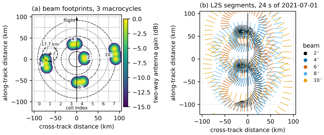
Figure 2.
Calibration of SWIM . (a) Daily drift correction per beam (shaded: commissioning, excluded; dotted: the 2022-08-17 gain step). (b) Incidence-dependent offset SWIM − GPM KuPR per beam, from direct collocations (no model involved). (c) Amplitude of the satellite-frame azimuth correction.
Figure 2.
Calibration of SWIM . (a) Daily drift correction per beam (shaded: commissioning, excluded; dotted: the 2022-08-17 gain step). (b) Incidence-dependent offset SWIM − GPM KuPR per beam, from direct collocations (no model involved). (c) Amplitude of the satellite-frame azimuth correction.
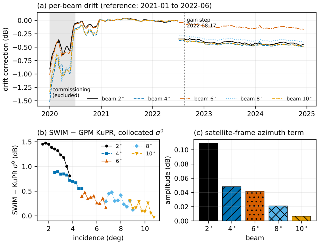
Figure 3.
Processing chain of the SWIM-only wind retrieval, from the L2S half-orbit to the level-2 wind product. The inversion uses the significant wave height of the SWIM nadir beam and passes the full direction likelihood to the ERA5-assisted variational analysis.
Figure 3.
Processing chain of the SWIM-only wind retrieval, from the L2S half-orbit to the level-2 wind product. The inversion uses the significant wave height of the SWIM nadir beam and passes the full direction likelihood to the ERA5-assisted variational analysis.
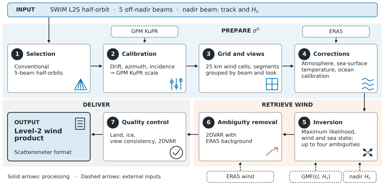
Figure 4.
(a) Fractions of the WVCs with views that are usable and rejected, per cross-track cell (bars), and frequency of each rejection cause (markers; a WVC may have several causes). (b) Usable WVCs per month.
Figure 4.
(a) Fractions of the WVCs with views that are usable and rejected, per cross-track cell (bars), and frequency of each rejection cause (markers; a WVC may have several causes). (b) Usable WVCs per month.
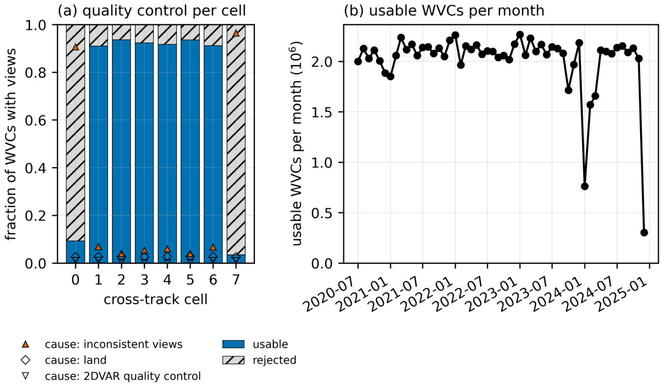
Figure 5.
Three SWIM segments of about 1250 km in an along-track frame (flight direction up); rows (a) 16 November 2020, (b) 20 December 2020, (c) 20 October 2021. Columns: (1) SWIM (WVCs that pass quality control), (2) the nearest ASCAT pass (KNMI, 12.5 km; time after SWIM in brackets), (3) ERA5 at the nearest hour, and the differences (4) ASCAT − SWIM and (5) ERA5 − SWIM on the SWIM cells (ASCAT averaged within km; ERA5 as the 2DVAR background). Colour: wind speed or difference; arrows: wind direction (unit length, pointing where the wind blows); dashed: the SWIM swath; grey: land.
Figure 5.
Three SWIM segments of about 1250 km in an along-track frame (flight direction up); rows (a) 16 November 2020, (b) 20 December 2020, (c) 20 October 2021. Columns: (1) SWIM (WVCs that pass quality control), (2) the nearest ASCAT pass (KNMI, 12.5 km; time after SWIM in brackets), (3) ERA5 at the nearest hour, and the differences (4) ASCAT − SWIM and (5) ERA5 − SWIM on the SWIM cells (ASCAT averaged within km; ERA5 as the 2DVAR background). Colour: wind speed or difference; arrows: wind direction (unit length, pointing where the wind blows); dashed: the SWIM swath; grey: land.
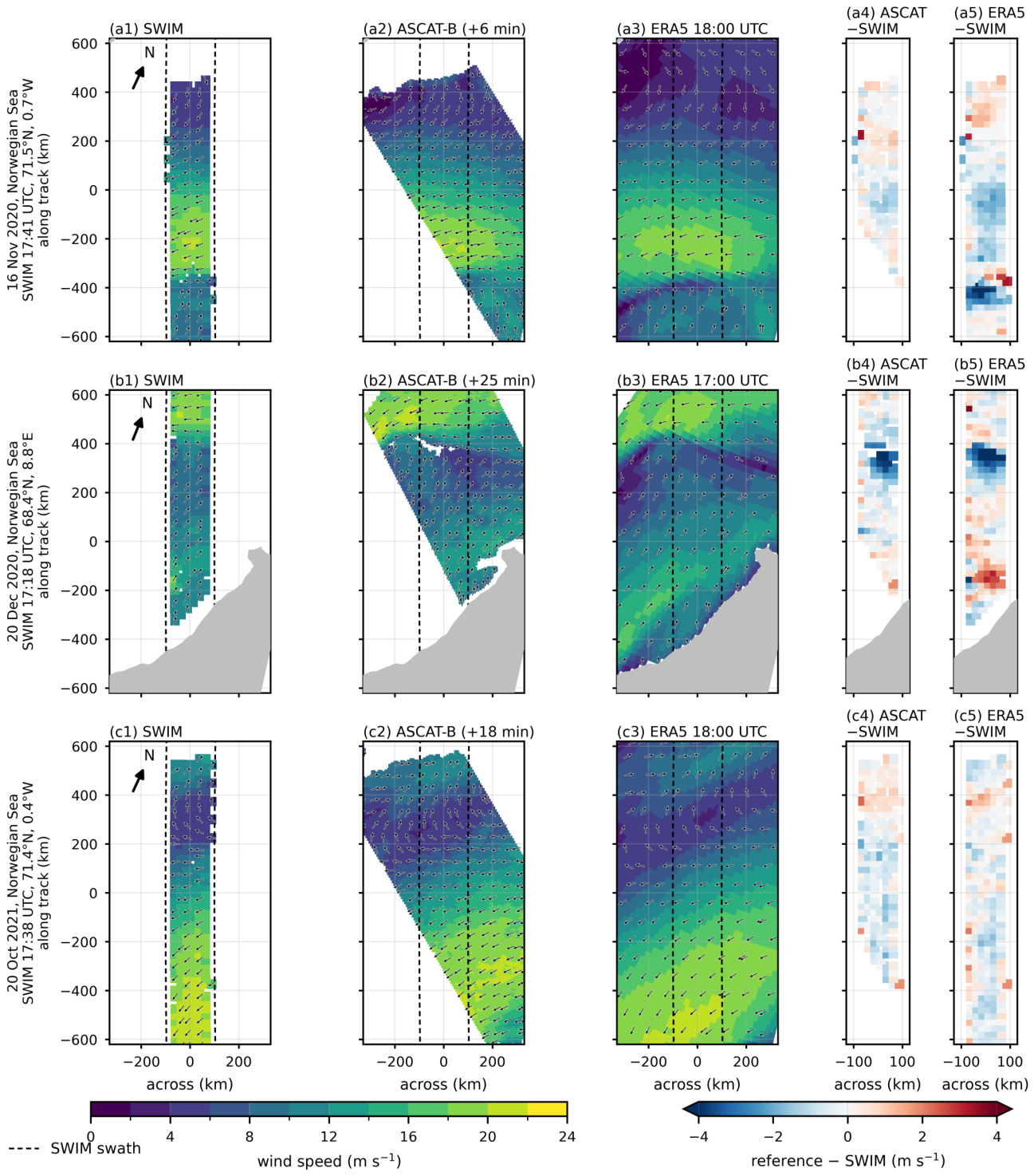
Figure 6.
Matches of SWIM (horizontal) with the references (vertical), all winds, logarithmic counts. Speed against (a) ASCAT and (b) the ERA5 background; (c) zonal and (d) meridional components against ASCAT. Insets: all-wind statistics, bias = reference − SWIM; dashed: one-to-one line.
Figure 6.
Matches of SWIM (horizontal) with the references (vertical), all winds, logarithmic counts. Speed against (a) ASCAT and (b) the ERA5 background; (c) zonal and (d) meridional components against ASCAT. Insets: all-wind statistics, bias = reference − SWIM; dashed: one-to-one line.
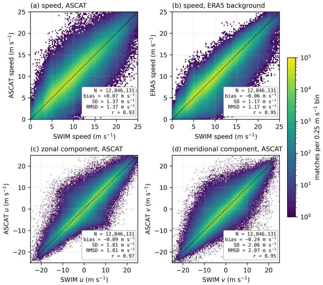
Figure 7.
Speed difference reference − SWIM in 1 m bins. (a) Bias against ASCAT, HY-2 and ERA5, each binned by the mean of SWIM and that reference, and against ASCAT binned by the ERA5 wind alone; (b) SD; (c) distribution of the ASCAT matches over the mean wind. (d) Bias and SD against ASCAT and HY-2 per cross-track cell (mean wind 4–20 m ).
Figure 7.
Speed difference reference − SWIM in 1 m bins. (a) Bias against ASCAT, HY-2 and ERA5, each binned by the mean of SWIM and that reference, and against ASCAT binned by the ERA5 wind alone; (b) SD; (c) distribution of the ASCAT matches over the mean wind. (d) Bias and SD against ASCAT and HY-2 per cross-track cell (mean wind 4–20 m ).
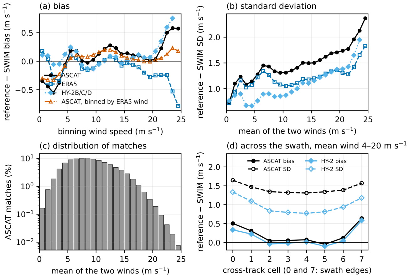
Figure 8.
Wind direction against ASCAT, mean wind above 4 m . (a) SWIM rank-1 and (b) selected direction (horizontal) against ASCAT (vertical), logarithmic counts. (c) Fraction of cells within of ASCAT for the rank-1 solution, the closest ambiguity, the selected solution and ERA5, in 1 m bins of mean wind; dotted: random direction (25 %). (d) Distribution of the direction difference ASCAT − SWIM.
Figure 8.
Wind direction against ASCAT, mean wind above 4 m . (a) SWIM rank-1 and (b) selected direction (horizontal) against ASCAT (vertical), logarithmic counts. (c) Fraction of cells within of ASCAT for the rank-1 solution, the closest ambiguity, the selected solution and ERA5, in 1 m bins of mean wind; dotted: random direction (25 %). (d) Distribution of the direction difference ASCAT − SWIM.
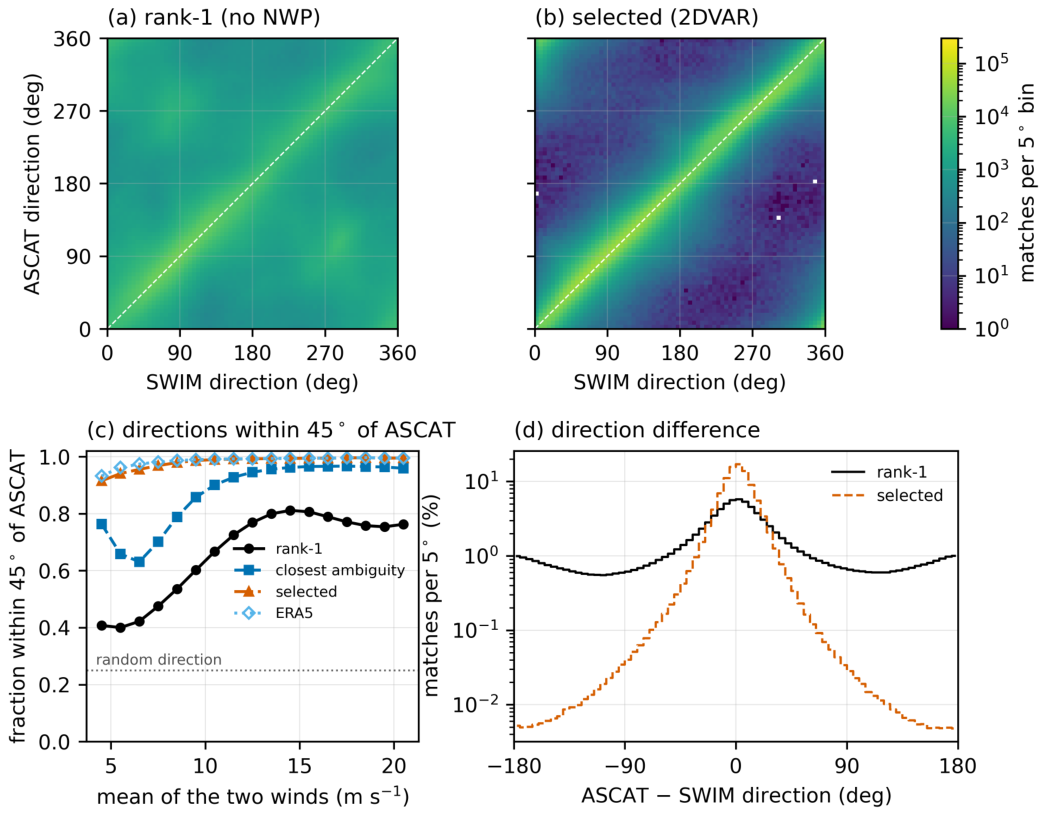
Figure 9.
Mean speed difference in bins (mean wind 4–20 m ), with the sea-state term (solid, filled) and with the wind-only model (dashed, open). (a) Buoys, all months, buoy ; ERA5 and HY-2 against the same buoys as controls. (b) ASCAT and HY-2 (20 % sample), held-out months, ERA. The last bin holds all above 6 m. Legend: slope on fitted with a separate offset for each 2 m class of mean wind (m per m). (c) The same slope within each 2 m class of mean wind, for buoy − SWIM, buoy − ERA5 and ASCAT − SWIM.
Figure 9.
Mean speed difference in bins (mean wind 4–20 m ), with the sea-state term (solid, filled) and with the wind-only model (dashed, open). (a) Buoys, all months, buoy ; ERA5 and HY-2 against the same buoys as controls. (b) ASCAT and HY-2 (20 % sample), held-out months, ERA. The last bin holds all above 6 m. Legend: slope on fitted with a separate offset for each 2 m class of mean wind (m per m). (c) The same slope within each 2 m class of mean wind, for buoy − SWIM, buoy − ERA5 and ASCAT − SWIM.
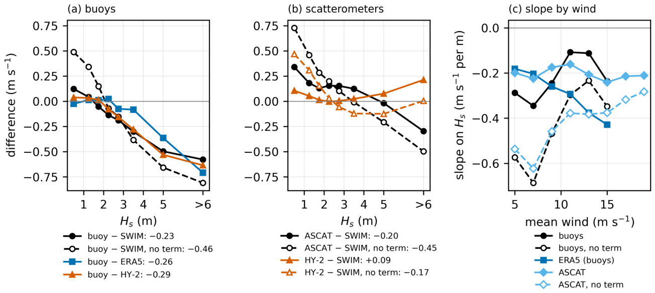
Figure 10.
Speed differences ASCAT − SWIM, ASCAT − ERA5 and ERA5 − SWIM on the ASCAT matches, and HY-2 − SWIM on the HY-2 matches (20 % sample), in the held-out months from 2021 with mean wind 4–20 m , against (a) latitude, (b) sea-surface temperature (SST) and (c) water vapour. Bars: nominal standard errors assuming independent matches, mostly smaller than the markers.
Figure 10.
Speed differences ASCAT − SWIM, ASCAT − ERA5 and ERA5 − SWIM on the ASCAT matches, and HY-2 − SWIM on the HY-2 matches (20 % sample), in the held-out months from 2021 with mean wind 4–20 m , against (a) latitude, (b) sea-surface temperature (SST) and (c) water vapour. Bars: nominal standard errors assuming independent matches, mostly smaller than the markers.
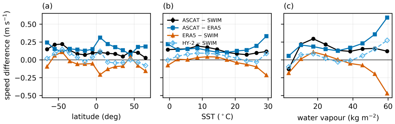
Figure 11.
(a) Monthly bias and SD of ASCAT − SWIM (markers) and HY-2 − SWIM (lines; 20 % sample), all winds, and (b) number of matches, over all months. Open markers: fit months, excluded from the other scatterometer statistics; dotted vertical line: the 2022-08-17 gain step.
Figure 11.
(a) Monthly bias and SD of ASCAT − SWIM (markers) and HY-2 − SWIM (lines; 20 % sample), all winds, and (b) number of matches, over all months. Open markers: fit months, excluded from the other scatterometer statistics; dotted vertical line: the 2022-08-17 gain step.
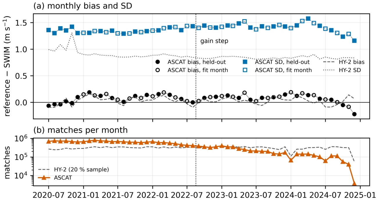

Table 1.
SWIM acquisition modes in the L2S v2.0/v2.1 record (half-orbits per beam combination, over the record and within 2020-07-01 to 2024-12-08).
Table 1.
SWIM acquisition modes in the L2S v2.0/v2.1 record (half-orbits per beam combination, over the record and within 2020-07-01 to 2024-12-08).
| Beams (deg) | L2S | Period | Half-orbits | In window | Use |
|---|---|---|---|---|---|
| 2, 4, 6, 8, 10 | v2.0/v2.1 | 2019-04 – 2024-12 | 35,843 | 28,644 | used |
| 2, 10 | v2.0/v2.1 | 2019-06 – 2026-06 | 10,448 | 687 | excluded |
| 2, 8 | v2.0 | 2019-06 – 2020-12 | 112 | 39 | excluded |
| 2, 8, 10 | v2.0 | 2019-07 – 2019-07 | 16 | 0 | excluded |
| 2, 4, 6 | v2.0 | 2019-07 – 2019-07 | 14 | 0 | excluded |
| 8 | v2.0 | 2020-11 – 2020-12 | 4 | 4 | excluded |
| 2, 4 | v2.0 | 2023-11 – 2023-11 | 1 | 1 | excluded |
Table 2.
Retrieved wind speed and components against ASCAT, HY-2 and ERA5 (54 months less the 24 fit months). Mean wind: mean of the SWIM and reference speeds (ASCAT for the ERA5 rows). Bias, SD and RMSD in m , reference − SWIM; , : SDs of the zonal and meridional components (selected direction), in m . HY-2 rows: random 20 % of the matches.
Table 2.
Retrieved wind speed and components against ASCAT, HY-2 and ERA5 (54 months less the 24 fit months). Mean wind: mean of the SWIM and reference speeds (ASCAT for the ERA5 rows). Bias, SD and RMSD in m , reference − SWIM; , : SDs of the zonal and meridional components (selected direction), in m . HY-2 rows: random 20 % of the matches.
| Reference | Subset | N | Bias | SD | RMSD | r | ||
|---|---|---|---|---|---|---|---|---|
| ASCAT | all winds | 12,846,131 | 1.37 | 1.37 | 0.93 | 1.81 | 2.06 | |
| ASCAT | mean wind 4– | 11,906,743 | 1.38 | 1.38 | 0.92 | 1.82 | 2.08 | |
| ASCAT Metop-B | mean wind 4– | 5,837,743 | 1.38 | 1.38 | 0.92 | 1.82 | 2.09 | |
| ASCAT Metop-C | mean wind 4– | 6,069,000 | 1.38 | 1.38 | 0.92 | 1.83 | 2.08 | |
| ASCAT | mean wind 4–, from 2021 | 8,054,026 | 1.38 | 1.39 | 0.92 | 1.85 | 2.10 | |
| HY-2B | mean wind 4– | 6,845,584 | 0.89 | 0.90 | 0.96 | 1.51 | 1.61 | |
| HY-2C | mean wind 4– | 1,380,771 | 0.92 | 0.92 | 0.96 | 1.53 | 1.67 | |
| HY-2D | mean wind 4– | 222,986 | 0.93 | 0.93 | 0.96 | 1.50 | 1.65 | |
| ERA5 (background) | all winds | 12,846,131 | 1.17 | 1.17 | 0.95 | 1.25 | 1.30 | |
| ERA5 (background) | mean wind 4– | 11,906,743 | 1.18 | 1.18 | 0.94 | 1.26 | 1.32 |
Table 3.
Wind speed against moored buoys for SWIM and the classical scatterometers, on the buoys and months that have a SWIM match (mean wind 4–20 m , each sensor at its own pass time). Bias and SD in m , buoy − sensor. TC error: triple-collocation error SD of the sensor (buoy, sensor, NWP), in m on the buoy scale. The CFOSAT scatterometer covers October 2020 to November 2022 only.
Table 3.
Wind speed against moored buoys for SWIM and the classical scatterometers, on the buoys and months that have a SWIM match (mean wind 4–20 m , each sensor at its own pass time). Bias and SD in m , buoy − sensor. TC error: triple-collocation error SD of the sensor (buoy, sensor, NWP), in m on the buoy scale. The CFOSAT scatterometer covers October 2020 to November 2022 only.
| Sensor | Band, antenna | N | Bias | SD | r | TC error |
|---|---|---|---|---|---|---|
| SWIM (this work) | Ku, near-nadir rotating beams | 19,277 | 1.36 | 0.89 | 0.83 | |
| ASCAT Metop-B | C, fan beams | 131,025 | 1.17 | 0.92 | 0.39 | |
| ASCAT Metop-C | C, fan beams | 129,683 | 1.16 | 0.92 | 0.40 | |
| HY-2B | Ku, rotating pencil beams | 191,693 | 1.18 | 0.92 | 0.43 | |
| HY-2C | Ku, rotating pencil beams | 207,392 | 1.23 | 0.92 | 0.48 | |
| HY-2D | Ku, rotating pencil beams | 48,405 | 1.27 | 0.91 | 0.46 | |
| CFOSAT SCAT | Ku, rotating fan beam | 44,720 | 1.42 | 0.89 | 0.80 |
Table 4.
Limits for use of the SWIM-only wind product (version 2.3).
| Condition | Recommendation |
|---|---|
| Period and mode | July 2020 to December 2024, conventional (5-beam) mode only. |
| Quality flags | Use only WVCs that pass quality control. |
| Swath | Inner six cells (about 150 km), cell 1 biased low; edge cells not recommended. |
| Wind speed | 4–22 m s−1 (ASCAT bias within 0. in mean-wind bins; SWIM about 0. below ASCAT, close to HY-2); below unreliable and high; above flagged, few matches. |
| Region | In the moist tropics SWIM reads low, by 0.1 to 0. against the scatterometers and 0. against buoys. |
| Sea state | Term driven by the SWIM nadir (ERA5 where missing); against buoys, residual dependence on similar to ERA5 and HY-2; over-correction relative to HY-2 (slope changes sign). |
| Direction | Selected direction depends on ERA5; the rank-1 solution measures SWIM’s own direction information, weak in light winds, and is not a stand-alone direction product. |
| Resolution | About 50 km, not the 25 km grid spacing. |
| Rain | No rain flag in this version. |
Disclaimer/Publisher’s Note: The statements, opinions and data contained in all publications are solely those of the individual author(s) and contributor(s) and not of MDPI and/or the editor(s). MDPI and/or the editor(s) disclaim responsibility for any injury to people or property resulting from any ideas, methods, instructions or products referred to in the content. |
© 2026 by the authors. Licensee MDPI, Basel, Switzerland. This article is an open access article distributed under the terms and conditions of the Creative Commons Attribution (CC BY) license (http://creativecommons.org/licenses/by/4.0/).
Copyright: This open access article is published under a Creative Commons CC BY 4.0 license, which permit the free download, distribution, and reuse, provided that the author and preprint are cited in any reuse.