

Submitted:
15 November 2026
Posted:
16 November 2026
You are already at the latest version
Abstract
Interference suppression depth alone does not determine the attitude accuracy of a global navigation satellite system (GNSS) antenna array. Starting from the physical--observation dual-axis (PODA) framework, we distinguish body attitude from the conditions under which observations are formed: channel calibration, filter coefficients, retained data dimensions, and temporal support. For proper complex Gaussian noise with fixed covariance and locally constant rank, we eliminate the unknown satellite amplitudes jointly and derive the full variable-projection Jacobian. The loss of attitude information separates into two terms: effective attitude tangents discarded by processing, and their overlap with nuisance-amplitude directions after compression. This decomposition gives a necessary and sufficient condition for preserving local attitude information. We then derive how direction errors, gain and phase mismatch, group-delay residuals, and finite-sample estimates of weights and covariance affect attitude estimation. The numerical study comprises 13,000 fits with known interference statistics, 6,400 fits with finite training and combined errors, and 4,500 channel-tolerance fits. Complete space--time and space--frequency representations of the same operator retain identical information; differences introduced by independent per-frequency constraints depend on the subspaces they remove. In a controlled calibration experiment, six dispersed satellites yield an attitude root-mean-square error (RMSE) of \(0.383^\circ\), compared with \(1.238^\circ\) for six clustered satellites. Finite-training experiments also show that accounting for residual interference correlation can substantially change attitude accuracy at the same null depth. These results establish information and sensitivity relationships under stated assumptions, supporting a joint assessment of effective attitude directions, model consistency, and residual statistics. A separate 62 MHz receiver-chain experiment examines carrier-reference consistency in RTK. In a representative coordinated turn, interference-free reception without correction and 95 dB interference with gyro-assisted phase transport each publish 100 fixes in 100 post-initialization epochs, compared with 41 for the uncorrected array branch. Published fixes and conditional integer verification are reported separately. These receiver results complement the attitude analysis; they do not establish virtual-gyroscope accuracy or measured product performance.
Keywords:
PODA
; GNSS attitude determination
; virtual gyroscope
; space–time adaptive processing (STAP)
; space–frequency adaptive processing (SFAP)
; array calibration
1. Introduction
As an unmanned aircraft rotates, the projections of its antenna baselines onto the satellite lines of sight change. The resulting relative carrier responses contain information about the aircraft’s attitude. Interference mitigation acts on those same responses by changing the combination of channels, their frequency weights, and the time interval represented by each observation. Once interference has been suppressed, the receiver therefore sees transformed data. If attitude estimation still uses the original response model, changes in gain and phase caused by filtering may be interpreted as body rotation. Even with a correct model, information removed by projection cannot be recovered through subsequent normalization.
Attitude estimation from interference-mitigated array data has an established research basis. Daneshmand et al. combined interference-subspace projection, array attitude recovery, and distortionless space–time filtering [1]. Marathe et al. examined the distortions that space–time processing introduces into GNSS measurements [2]. Distortionless space–frequency constraints and polyphase decomposition address related problems through response constraints and implementation structure, respectively [3,4]. For precise carrier measurements, phase compensation for blind spatial filtering and specific space–time constraints have also been reported [5,6]. Array calibration studies show, in turn, that direction-dependent gain and phase, mutual coupling, and differences between radio-frequency channels affect both the array response and the estimated attitude [7,8].
These studies explain how particular processing structures can reduce distortion. A further question concerns the information that survives processing: when the common complex amplitude of each satellite is unknown, which components of three-axis attitude remain observable, and how do direction, channel, and training errors propagate through the same observation chain? Output signal-to-noise ratio, the deepest pattern null, and satellite count alone do not answer this question. They do not account for the elimination of nuisance parameters or for weak directions in the attitude geometry.
We take the physical–observation dual-axis (PODA) structure as the starting point for the model [9,10]. On the physical axis, R describes the rotation of the array relative to the navigation frame. On the observation axis, specifies the channel responses, interference-mitigation weights, time window, and readout, giving . In this setting, the distinction requires every change in processing to enter the predicted response, noise statistics, and attitude derivatives consistently. Complex Gaussian estimation, variable projection, and differential calculus on the rotation group provide the mathematical tools used below; their sources are cited separately from the array-processing literature.
Earlier work on PODA phase transport in GNSS receiver chains focused on carrier references, dynamic tracking, and real-time kinematic (RTK) positioning [11]. Here the focus is the identifiability of attitude from multichannel observations: after the phase reference has been handled, which attitude directions remain in the data?
To answer this question, we derive a local information-loss decomposition and a preservation criterion in the presence of unknown complex amplitudes. The derivation distinguishes equivalent complete time- and frequency-domain representations from processing restricted to particular structures. Direction errors, gain and phase mismatch, group delay, and errors in forming the weights then enter as changes in the processed response and its statistics. Paired trials with shared inputs test these relationships while retaining large-error outcomes under finite training and weak geometry. The contribution lies in this consistent treatment of array attitude estimation, the information-preservation criterion, and the paired analysis of distinct error sources.
The term “virtual gyroscope” denotes the observation branch that obtains attitude from GNSS array responses. The main experiments measure attitude error on , using finite complex observation blocks under the assumptions in Section 7. Section 10 adds a separate RF-to-RTK experiment to examine the navigation branch in Figure 1. Its phase-transport branch is aided by a physical gyroscope. Position error and integer fixing are therefore reported as downstream carrier-observation outcomes, not as measurements of virtual-gyroscope attitude or angular-velocity accuracy.
1.1. Attitude Records and Performance Measures
A navigation output and a multichannel attitude record may be drawn from the same array, but they serve different purposes. Let be the combined navigation response. As approaches zero, its carrier phase becomes unstable; a separate branch retaining multichannel data may nevertheless retain attitude information. Conversely, a high signal-to-noise ratio in one combined output does not establish that sufficient relative information between elements survives. The assessment must follow the record actually supplied to the attitude estimator.
The overall error between the true attitude R and its estimate is the shortest rotation angle,
Here Log takes the principal rotation value and ∨ maps a skew-symmetric matrix to its three-dimensional vector. Overall error and the roll, pitch, and yaw components describe different aspects of performance; neither replaces the other. Component errors also require a stated Euler-angle convention. The experiments report the overall error distribution and the three components, retaining every failed or large-error trial.
Figure 2.
The four-element square with half-wavelength spacing and the twelve satellite lines of sight. The array is shown in body coordinates, with element 0 as the reference. Satellite azimuth is measured eastward from north, and radial position gives zenith distance. The figure is generated from the experimental geometry; the six-satellite configurations are specified in the numerical section.
Figure 2.
The four-element square with half-wavelength spacing and the twelve satellite lines of sight. The array is shown in body coordinates, with element 0 as the reference. Satellite azimuth is measured eastward from north, and radial position gives zenith distance. The figure is generated from the experimental geometry; the six-satellite configurations are specified in the numerical section.
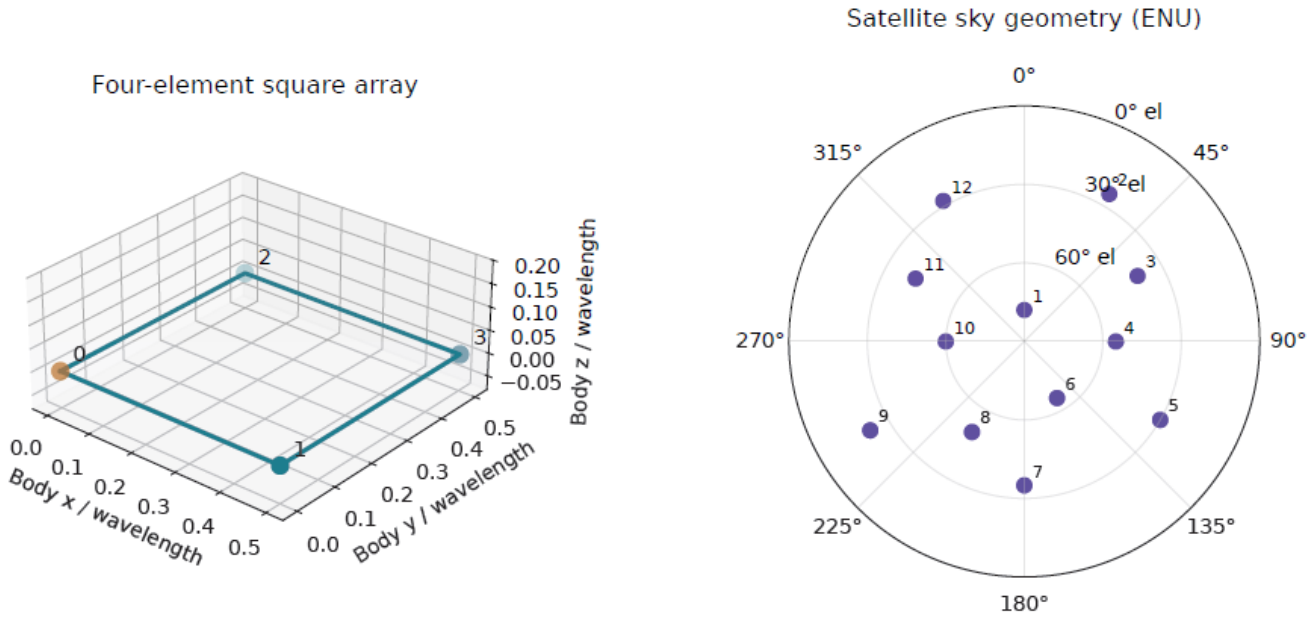
This array layout, the L1 carrier frequency, and the controlled satellite geometry define a reproducible joint complex observation block. The same realization of noise and interference can then be supplied to each processor. Block-energy ratios, training protocols, and observation normalization are stated for each experiment. They are not interchangeable with an interference-to-signal ratio at the radio-frequency input, and these attitude experiments do not replace full-chain receiver results. Measured direction-error distributions, null depth across the band, temperature-dependent calibration matrices, and saturation records remain separate inputs needed to apply the model to a product.
The distinction between the two observation branches also motivates the receiver-chain experiment in Section 10: a loss of integer-fixing availability need not imply a corresponding loss of multichannel attitude information, and a high fixing rate cannot certify attitude accuracy.
2. A Joint Model of Physical Attitude and Observation Conditions
2.1. Complex Array Response and Its Attitude Derivative
Consider an array of M elements observing S satellites at L frequency points. Let denote the baseline from the reference element to element m in the body frame, with . The rotation maps body-frame vectors into the navigation frame, and is the unit line-of-sight vector to satellite s in the navigation frame. At frequency , the geometric response is
Equation (2) fixes the propagation-phase sign convention used throughout; is the propagation speed. The actual channel is described by , which includes the radio-frequency chains, mutual coupling, element directional responses, and temperature . For known waveform coefficients , define the joint response
Stacking the element responses frequency by frequency gives and . The channel matrix may be factored to suit the calibration method, for example as ; the statistical analysis requires only the resulting response and its derivatives. The importance of direction-dependent calibration in precision array processing is discussed in [7,8].
Each satellite has one unknown complex amplitude within an observation block, accounting for both its amplitude and its common carrier phase over that block. The raw observation is
Satellites may share the same record, so the response columns need not remain orthogonal after processing. Statistics computed separately for each satellite must retain any cross-satellite correlations that are present. Assigning an arbitrary independent phase to each element would also eliminate the geometric phase to be identified. Assigning an independent complex amplitude to each satellite at each frequency would change the information available across frequencies. These choices define different observation models and cannot be interchanged without explanation in an algorithm comparison.
If a known kernel has already formed satellite-specific statistics, the finite record is the single-satellite case of Equation (4):
The vector may still contain several elements and frequency points; separation by satellite does not make it a single complex scalar. Nor does the separation kernel guarantee independent errors across satellites. When they share raw samples, their cross-covariance must follow from the actual kernels. Residual interference with a nonzero mean belongs in the mean-mismatch model and cannot be represented merely by increasing .
We use a right-multiplicative attitude perturbation, , where . Since
the first-order changes in geometric phase and response are
If depends on the body-frame direction , the channel response must also be differentiated using :
Here denotes the directional derivative of the matrix-valued function. The second term vanishes for a fixed, direction-independent calibration. Local coordinates and Jacobian conventions on the rotation group follow [12]. When the implementation parameterizes attitude by a rotation vector, the corresponding right Jacobian is also required: the coordinate derivative with respect to a finite rotation vector is not itself the derivative with respect to a right-multiplicative perturbation.
The derivatives also expose a basic geometric limitation. For a single satellite and direction-independent channels, rotating the array about the satellite’s line of sight in the navigation frame leaves the geometric response unchanged:
The corresponding right-perturbation direction is ; substituting it into Equation (7) gives zero phase change. A stronger signal cannot resolve this unobservable direction. Whether several satellites jointly constrain all three rotation axes depends on the rank of the processed joint Jacobian, not on satellite count alone.
A single-baseline model makes the same dependence explicit. Let be a horizontal baseline length, the line-of-sight azimuth, and the horizontal angle to be estimated. Then
The second expression requires a nonzero denominator and a sufficiently small perturbation. The same phase residual can therefore produce different angular errors under different geometries. Near a direction of zero sensitivity, this local inversion itself fails. Neither phase quality nor null depth alone determines three-axis attitude accuracy.
2.2. Processing Operators, Temporal Support, and Noise Support
For the processing matrix A actually implemented, the coherent output satisfies
This observation equation underlies the analysis that follows. The conditional information analysis treats interference statistics as given in the body frame, so does not depend on the candidate attitude. If an interference direction known in the navigation frame is used instead, the covariance may vary with attitude; its derivatives then contribute additional information to the likelihood and require a separate model. The output record, candidate response, and covariance must all use the same A. For example, reference-channel regression retaining residual channels has . Even with white input noise, the shared reference channel induces correlations in the output noise.
For four channels, write the instantaneous array response as . Reference regression then gives
The last identity assumes unit white input noise and shows the shared reference-noise contribution to the three residual outputs. Temporal regression additionally requires the regression kernel and its time moments; the instantaneous spatial equation cannot replace the full finite-window model.
When , . Choose an orthonormal basis E for this range and set and to whiten the observations on their effective support. We henceforth work directly in these effective output coordinates, in which K is positive definite. Deterministic noise constraints or an attitude-dependent support require their own likelihood; the fixed-support formulas do not apply unchanged.
Spatial processing (SP) uses the same spatial map at every frequency, whereas frequency-wise space–frequency (SF) processing selects a separate spatial map at each frequency:
If the orthonormal columns of span the spatial interference subspace, an orthonormal complement gives
The independent residual coordinates produced by B contain the same effective record as in the original coordinates; the latter usually has a singular output covariance. A common spatial map removes the same direction at every frequency. It cannot exploit spectral differences to preserve information in other bands, and may fail to maintain a null across the band if the interference response varies appreciably with frequency. Its attitude cost is set by the sensitive directions removed, not by a fixed equivalence to losing one element.
Frequency-wise processing can treat bands differently without making them statistically independent. If denotes a frequency block of the input covariance, then
Discarding these off-diagonal blocks is a covariance approximation, not a property of the Fourier transform. Allowing a separate unknown amplitude for every satellite at every frequency also removes cross-frequency constraints. The nuisance-parameter definitions must therefore be held fixed when processing methods are compared.
For a space–time record, the stacking order is
The operator can couple both elements and epochs. Choosing the orthogonal complement of the joint interference subspace gives several coherent outputs. Conventional single-output beamforming, , instead forms a main navigation channel. Whether that output also supports attitude estimation depends on other retained observations or cross-block constraints, not on its interference-suppression capability alone.
Space–time (ST) processing applies to a joint record over elements and time. A finite impulse-response kernel has frequency response
If body rotation over the window is appreciable, the correct mean depends on past attitudes:
Code correlation, the numerically controlled oscillator (NCO), and the integration window can be incorporated into the temporal kernel. The frequency response and measurement distortions induced by space–time filtering have been studied in [2]; Equation (18) also makes explicit the physical epochs represented by an attitude observation.
Let , where is the unitary discrete Fourier transform (DFT) matrix. For the same finite record, if
then the two representations give exactly the same , and therefore the same likelihood and attitude estimate. A frequency-wise independent structure cannot, in general, represent an arbitrary . Neglecting cross-frequency covariance, truncating filter taps, or changing boundary treatment also changes the estimation problem. Equivalence of complete representations does not imply equivalence of all STAP and SFAP implementations; linear convolution must likewise be distinguished from circular convolution without zero-padding [3,4].
The equivalence can also be checked term by term:
A further unitary output transformation leaves the likelihood unchanged when , , and are used together. Practical comparisons must specify tap or FFT length, training records, loading, windows, boundary treatment, and output count. The meaning of a comparison between processing domains depends on these choices.
If angular velocity or other motion parameters are introduced to model a dynamic finite window, they must be eliminated as nuisance parameters or estimated jointly unless independently known; attitude is then evaluated at the specified epoch. Equation (18) does not assume an available gyroscope input. The main numerical comparisons freeze attitude within each block and do not evaluate additional errors from rapid motion across the window.
2.3. Phase Transport and Attitude Information
For a scalar combined output, let be its nonzero complex response. On a smooth local region containing no response zero, the phase-transport one-form is [10]
The two terms express, at the level of response phase, the PODA distinction between a change in attitude and a change in the conditions under which the observation is formed. Integrating a continuous phase along a path requires a nonzero response and a continuous phase lift; a closed-path integral may contain an integer multiple of associated with winding. When weights switch from old to new values at the same physical state, the relative phase between nonzero responses is . Compensation must use the same signal epoch and phase reference.
Equation (21) describes how a known complex response changes. By itself, it neither identifies unknown channel errors nor restores spatial dimensions discarded by the processor. To determine how much attitude information remains after compensation, we first eliminate the common complex amplitudes of the satellites, which do not encode relative spatial structure, and then examine the attitude derivatives of the remaining response.
3. Eliminating Complex Amplitudes and Preserving Attitude Information
3.1. Variable Projection and Its Full Derivative
Condition first on fixed A and K. Assume that is proper complex Gaussian noise and that K does not vary with the parameters in the attitude neighbourhood under consideration. Choose and define
Equation (22) is the negative log-likelihood up to an additive constant. For fixed R, the normal equation gives
Here is the Moore–Penrose inverse. This elimination is the variable-projection method for separable nonlinear least squares [13]. The derivatives below assume that C has full column rank locally and that W is fixed; points at which the rank changes require separate treatment.
Write . Differentiating and the normal equation gives, respectively,
Substitution into the first equation yields the full derivative of the projected residual:
The second term is generally nonzero when the residual is nonzero. Retaining only the first term is an approximation and should not be identified with the full variable-projection derivative. Stacking the real and imaginary parts of r and permits the use of real nonlinear least squares, with local Gauss–Newton equation
An iteration using right-multiplicative local increments updates attitude as
Local convergence does not guarantee global uniqueness. Initialization, phase periodicity, and geometric symmetries can still determine the solution branch. Large-error and nonconverged records must therefore be retained rather than scoring only successful fits.
Equation (27) defines the local step; it does not require an implementation to form the normal matrix explicitly. The numerical implementation uses trust-region least squares in a rotation vector p, converting Equation (7) to a coordinate derivative with respect to p through the right Jacobian. This differs from an implementation that applies a right-multiplicative update at each iteration. Amplitudes are currently obtained from a small Gram system, which requires the response matrix to retain adequate column rank. Near rank loss, a rank-revealing QR factorization or singular value decomposition (SVD) is preferable, together with rejection of records that provide no effective attitude constraint.
Holding the weights fixed during differentiation is distinct from ignoring their randomness. If A, the projection, or the whitening matrix W is recomputed for every candidate attitude, its derivatives must also enter the objective. Using Equation (26) while treating those quantities as constant would solve a different problem. Conversely, differentiating the candidate response with saved weights does not remove their training uncertainty from the final error assessment; its propagation is considered in Section 5.
3.2. The Effective Attitude Tangent Space and Local Information
At the true parameters, define the whitened attitude derivatives
The linearized mean is . Arbitrary infinitesimal amplitude changes lie in , so only constrains attitude independently of amplitude. Eliminating the real and imaginary parts of the complex amplitudes as nuisance parameters gives
The factor of two accounts for the two real components of proper complex Gaussian noise. The same expression follows by fixing a real attitude direction d and minimizing the squared norm of the mean change over .
Positive definiteness of establishes regular local identifiability of all three attitude components on the chosen branch. For an estimator satisfying local unbiasedness and the usual regularity conditions, the Cramér–Rao bound (CRB) gives
The second bound concerns unbiased error in fixed local coordinates. Comparing it with the RMSE of the total rotation angle also requires a small-angle approximation; it does not predict the incidence or magnitude of large-angle errors. Phase periodicity, reflection ambiguities in planar arrays, and multiple nonlinear modes may still produce solutions far from the selected branch. The smallest eigenvalue measures the weakest local rotation direction, whereas the condition number measures only the imbalance between directions. They should therefore be reported separately.
If each satellite contributes only one complex scalar per block, with a free complex amplitude assigned to that scalar, any nonzero response has . Its attitude information is zero. Adding scalar blocks with their own free complex amplitudes does not remove this degeneracy unless reliable constraints are imposed across blocks or spatial dimensions are retained elsewhere. A high signal-to-noise ratio in a single combined navigation signal is therefore insufficient evidence of attitude-estimation capability.
3.3. Explicit Single-Satellite Elimination and Conditions for Combining Satellites
Consider one satellite-specific block from Equation (5). After processing, . Choose on the effective noise support and write
For fixed R, setting the derivative of with respect to to zero gives . Hence
These expressions require . A zero-response block cannot be recovered by normalizing a common amplitude. Its ineffective constraint must be removed, or a full model must explicitly handle zero responses and rank changes.
The first-order change in the single-satellite mean is
The unknown amplitude absorbs complex changes along . Only the projected change constrains attitude independently. It follows that
This is the single-column case of Equation (30). The sum is valid only when satellite records are independent and the covariance has the corresponding block-diagonal structure. For a shared joint record, response columns can overlap: amplitude elimination must project against all of , rather than project each satellite separately and add the results.
The information condition number must also be distinguished from absolute accuracy. Scaling down all sensitivities can leave the condition number unchanged while increasing the error bound. If information is rank deficient, adding diagonal terms to its matrix does not supply the missing attitude direction to the observations. Damping can stabilize an iteration, but is not additional observational information.
3.4. A Two-Term Decomposition of Information Loss
Whether a processor preserves attitude information can be determined directly in the raw whitened coordinates. Define
The three columns of V are the effective attitude tangents after amplitude elimination. The projector P selects the whitened row space retained by the processor, and Q selects the processed amplitude directions. Since , we have .
16
Proposition 1
(Conditional preservation of local information). Suppose that the raw noise is proper complex Gaussian, with independent of attitude in a parameter neighbourhood. Let the processing matrix A be fixed and independent of the noise in the current measurement. At a regular operating point where the relevant ranks are locally constant, the information after eliminating the unknown complex amplitudes satisfies
The full three-dimensional local information is preserved if and only if
Proof.
Whitening after processing is equivalent to projecting the raw whitened record onto and then choosing orthonormal coordinates on that space. For any real direction d, amplitude elimination further removes . Since ,
Because is an orthogonal projector, the squared norm of the effective mean change in direction d gives the quadratic form in Equation (37). Subtracting this from the raw information yields Equation (38).
If information is fully preserved, then for every real d. Taking the three coordinate directions gives . Conversely, if , then , so and both loss terms vanish. □
The first term in Equation (38) measures effective attitude directions discarded directly; the second measures their overlap with amplitude directions after compression. The decomposition applies projection algebra and nuisance-parameter elimination to array attitude estimation. It imposes a stronger requirement than preserving useful-signal power: preserving the nominal response does not ensure that its effective attitude derivatives are preserved. A direct counterexample retains only in the raw whitened space and discards a nonzero V orthogonal to it. The nominal signal is preserved exactly, yet all attitude information is lost.
The same monotonicity also follows directly from a minimization. For every real attitude direction d,
Here already includes the true complex amplitudes. Orthogonal projection cannot increase the norm for any candidate nuisance change, and the inequality survives minimization over those changes. Equation (38) identifies the two sources of the reduction and the condition for equality.
An invertible operation has and preserves information. A noninvertible operation is lossless only when Equation (39) holds. The benchmark here is an ideal estimator using the raw observations and the full covariance . In a practical receiver with approximate statistics, limited dynamic range, or computational constraints, interference mitigation can still reduce the actual estimation error. This is consistent with .
A nominal response constraint fixes only the response value. Protecting attitude information also requires examination of and of the directions remaining after amplitude elimination. Protecting both responses and derivatives consumes additional degrees of freedom and depends on the accuracy of the nominal attitude and calibration. We use this observation as a design criterion; the corresponding constrained optimization has not been solved or validated here as an algorithm.
3.5. Waveform Projection, Normalization, and Noise Amplification
A conditional waveform model shows why normalization cannot undo the removal of useful signal. Let , where is a nonzero temporal waveform. Given a full-row-rank reference matrix Z, define
The matrix projects onto the orthogonal complement of the reference temporal subspace. Projection followed by the matched kernel gives
Suppose that, conditional on Z, the temporal columns of remain independent with common spatial covariance . Using then gives
Dividing by restores the mean scale, but increases the standard deviation by relative to . At , the waveform has been removed completely and the division is undefined. If Z is learned from the same noisy record, the conditional noise assumption must first be checked; this covariance formula cannot be carried over automatically. The scalar example explains the loss from waveform projection. A moving observation window also changes sensitivities differently along the rotation axes, so one retention factor cannot replace the full attitude information matrix.
4. Constrained Minimum-Power Design and Protection of Attitude Information
Subspace projection makes the retained directions explicit, whereas practical interference-mitigation weights are also often obtained by minimizing output power. Regardless of how the weights are formed, attitude assessment must use the same processed observation equation: transform the output, candidate mean, and covariance together, then eliminate the unknown complex amplitudes.
Let the spatial, space–time, or space–frequency input be , with design covariance . A weight matrix forms r outputs, . The subscript distinguishes the design weights from the whitening matrix W. The columns of specify the response directions to be constrained, and specifies their targets. The linearly constrained minimum-variance (LCMV) problem is
With a complex matrix multiplier , the Lagrangian is
Differentiation with respect to gives the stationarity condition . Positive definiteness of implies ; substitution into the constraint yields
If has full column rank, the middle matrix is positive definite and the unique minimizer is
The positive-definite objective is strictly convex along feasible directions, so this stationary point is the minimum. Dependent constraint columns require a compatibility check and removal of redundancy; a singular matrix inverse is not a valid design.
For , , and , Equation (48) reduces to the minimum-variance distortionless-response (MVDR) weights:
The nominal response must be known or supplied by a prior. If it depends on the attitude being estimated, the prior attitude or the actual iterative construction must be specified. Forming the constraint with the true attitude and then claiming to recover that unknown attitude from the output would leak truth into the comparison. The main subspace experiments here do not use the true satellite attitude to construct such constraints.
Spatial design solves the problem in M dimensions; joint space–time design uses dimensions; common frequency-wise designs solve L separate M-dimensional problems. For a complete joint record, let and transform the design consistently:
Equation (48) then gives , so . Retaining only diagonal frequency blocks of the covariance, or restricting constraints to independent frequency-wise forms, changes the design problem. It agrees with the complete joint solution only under the corresponding structural conditions.
A distortionless constraint fixes the nominal response value. Attitude also depends on the neighbouring derivatives and on the directions that survive amplitude elimination. To protect both response and local sensitivity, independent columns from these quantities can be assembled into , with compatible output targets in ; for example, a column in has target row . Feasibility depends on constraint rank, output dimension, and the remaining interference-mitigation degrees of freedom. Additional constraints consume space available for null formation, while inaccurate nominal attitude or calibration can misalign the protected directions. Preserving response and derivative values does not remove the need to examine the actual noise covariance and Equation (39).
For fixed noise statistics, the weakest attitude direction can also be made the design objective directly:
The class specifies r output dimensions and realizable operator structures. Orthonormal rows fix the output gain and prevent a trivial reduction of the weights from appearing to satisfy the power constraint. The matrix must use the transformed mean and full covariance, with all complex amplitudes allowed by the model eliminated. This formulation places residual interference, information retention, and implementation constraints in one problem. It has not been solved here and is not included in the numerical algorithm ranking. It is a testable objective for subsequent design; the present experiments evaluate explicitly specified processing subspaces.
5. Propagation of Direction, Channel, and Training Errors into Attitude
5.1. Null Leakage and Desired-Signal Loss
Nulls designed from an estimated direction of arrival (DOA) and nulls learned directly from a sample covariance are affected by different errors. The former depend explicitly on an angle estimate. The latter need not produce an angle estimate at all, but remain sensitive to subspace estimation, nonstationary training data, and changes in the channels.
Consider a single frequency. Suppose the design satisfies , while the true interference response is and the implemented operator is . A first-order expansion gives
Direction, channel, and implementation errors add as complex amplitudes and can reinforce or cancel one another. Their powers cannot simply be added without further assumptions, such as independent zero-mean errors.
Let a denote azimuth measured eastward from north in the east–north–up (ENU) frame, and let e denote elevation. The corresponding unit vector v and its first-order perturbation are
Hence . A given angular error produces different leakage for different baselines and arrival directions. Near zenith, the angle between unit direction vectors is a more appropriate measure than azimuth error alone.
Null depth must be defined at a fixed reference plane. For an operator with orthonormal rows, , define the retained energy fractions by
With the same integration interval and bandwidth at the input and output reference planes, the interference-to-signal ratio obeys
For general weights, the noise gain or gain in a reference direction must also be specified. Suppression of total energy across several outputs is not the same as the deepest null in a single beam pattern. Nor can suppression at the center frequency stand in for the worst case over frequency, angular offset, and elapsed time since a weight update.
A two-element array with half-wavelength spacing gives a simple check. With angle measured from broadside, let the response be . Unit-norm weights that place an exact null at yield
For and an error of , the normalized null depth is 51.24 dB. This value applies only to the stated two-element example. Even when two processors have the same , they can differ in , the effective tangent space V, and output noise correlation. Attitude accuracy therefore cannot be determined by alone.
5.2. Gain and Phase Mismatch and Attitude Bias at a Specified Epoch
For the diagonal channel residuals used in the numerical study, take the phase at the carrier frequency to have been calibrated and write
Here is in decibels, is in radians, and is a differential group delay. The group delay multiplies only the frequency offset , so that the calibrated carrier phase is not counted twice. Gain changes can also alter the phase of a complex channel combination. Residual group delay, directional response, and mutual coupling across the band cannot be represented fully by a single carrier-phase error.
Carrier phase, differential delay, and the remaining in-band phase variation can also be separated explicitly by writing , with . Under the chosen delay-calibration convention,
Here records the frequency-dependent phase shape not explained by the selected linear-delay term. Correcting one phase value at the carrier does not determine that shape across the band. Mutual coupling, directional response, and temperature changes may also invalidate a previously measured calibration matrix. Calibration may measure the combined channel matrix directly, without identifying every physical contribution separately, but the model must retain the relative changes that affect attitude inversion.
Let b be the difference between the true mean and the mean predicted by the estimation model. With a fixed weighting matrix, eliminating the amplitudes gives
This follows from the local normal equations for and requires small mismatch, full rank, and the correct local solution branch. A common complex gain lying in is absorbed by amplitude elimination; relative channel residuals generally are not. A weak information direction amplifies only the error projected onto that direction. The condition number cannot be used as a universal multiplier for an arbitrary phase error.
If the implemented operator differs from the one used in estimation, or the true channels differ from the calibration model, the first-order mean mismatch is
The last term accounts for an unmodeled coherent interference mean. If the actual quantized weights are fully included in the candidate response, there is no arising from a discrepancy between the implemented and recorded weights. Quantization can still change the null and the information retained, but does not by itself imply a response-model bias.
In the single-satellite model of (18), is a common scalar amplitude. Let and . Over a short window, take , where is the body-frame angular velocity at the target epoch. If the common amplitude is approximately constant, expansion with gives
The first temporal moment converts motion within the window into a response mismatch at the target epoch, which then propagates through (59). A common pure delay can be handled by assigning the correct measurement epoch; differential delays generally cannot be removed by a single time shift. Attitude is frozen within each block in the attitude-block experiments, so (61) is not presented as a validated model of dynamic performance.
5.3. Finite Training and a Misspecified Weighting Matrix
Suppose the covariance is estimated from independent, stationary snapshots. Before loading, the sample matrix is
The training statistics represent the measurement epoch only when the process is sufficiently stable and the sampling conditions are appropriate. For an isolated dominant eigenvalue with unit eigenvector , first-order subspace perturbation gives
Leakage thus depends on the eigengap, sampling error, and any subspace change by the measurement epoch. Adding a scalar multiple of the identity does not change the eigenvectors. Its benefit to the numerical conditioning of covariance inversion must therefore be distinguished from subspace correction. Satellite components in the training data may also contaminate the residual statistics; a training window free of desired signals cannot be assumed without justification.
Equation (63) gives a first-order contribution to interference-leakage amplitude; the corresponding leakage power is second order in the perturbation amplitude. A small eigengap, too few samples, a narrowband source whose frequency changes between windows, or body rotation during training may all increase the discrepancy between the true and estimated subspaces. Trials that reuse ideal weights and resample only the test noise do not include this adaptation error.
Denote the training and independent validation records by . When the processor and weighting matrix are obtained from , they can be held fixed while differentiating the candidate response. If the test record is independent, its estimation error can first be analyzed conditional on . This conditional likelihood does not include any additional attitude information that the training records themselves may contain. If the same record is used both to learn A and to estimate attitude, the differential must instead include
and the dependence between the weights and the data must be retained.
When estimation uses while the true covariance is K, the matrix in (30) constructed from describes only nominal local sensitivity. Its inverse does not, in general, give the error covariance of a misspecified estimator [14,15]. Let be the real-valued profile residual, , , and the estimating function. At the conditional pseudo-true parameter satisfying , define
For a consistent M-estimator based on n independent, identically distributed blocks and satisfying local regularity conditions, the asymptotic covariance is . If the residual at the pseudo-true parameter is nonzero, the second term in the Hessian cannot generally be neglected. Only under a local linearization with small residuals does this reduce to the single-block propagation approximation
where is the true covariance of the same real-valued residual. When the projected residual is retained in its original ambient dimension, contains the projection structure and cannot automatically be set to the identity. Equation (67) does not characterize error statistics reliably under severe mismatch, multiple solution modes, or large attitude errors.
In a common local coordinate system, training randomness contributes to the total error through the law of total covariance:
Inverting or averaging nominal information matrices alone misses the second term. The experiments in Section 7 retrain the processor in every trial and evaluate rotation errors directly on , rather than extending a local covariance approximation into a regime of large errors.
5.4. Satellite Geometry and Directional Error Propagation
The matrix D in (30) includes the satellite lines of sight, array baselines, frequencies, powers, and actual channel responses. Weak satellites, satellites close to a null, and directions with uncertain calibration cannot simply be assigned the same weight as strong, stable observations. Satellite count is also no substitute for examining three-axis information. The smallest eigenvalue, all three eigenvectors, the local error ellipsoid, and the observed attitude RMSE together characterize the geometry.
For a nearly horizontal planar array, lines of sight clustered near zenith can make the baseline projections relatively insensitive to rotation about the array normal, so yaw may be the first weak direction. When the lines of sight are concentrated on one side, the weakest direction may instead combine several rotation axes. That direction must be computed from the processed information matrix. Neither a large satellite count nor a small position dilution of precision guarantees stable three-axis attitude estimation.
Direction errors, channel bias, and satellite geometry interact through the same effective attitude directions. Equal residual interference powers can produce very different attitude errors when they affect different directions. A deterministic mean mismatch is projected, whitened, and propagated from (60) through (59); random errors require their actual covariance and correlated cross terms. The two contributions should be evaluated separately under the same attitude-error definition before being combined into mean-square error. Several nominal error magnitudes cannot simply be added as independent contributions.
6. Null-depth Budgets for Direction, Gain, and Phase Errors
Equation (56) provides an independently checkable error scale. Consider a two-element array with half-wavelength spacing, a null designed at broadside, and an actual direction offset . With unit-norm weights and normalization by the true total input interference energy, the retained fraction is . Table 1 evaluates this expression to show how a deep null deteriorates with direction error. The example contains neither the directional patterns and mutual coupling of an actual four-element array nor its broadband calibration, so the suppression values are not product specifications.
The input value of 95 dB is simply a substitution into (55). The output interference-to-signal ratio equals the input ratio minus interference suppression plus desired-signal loss. No despreading or correlation-integration gain for a particular interference signal has been included. Two nominal 50 dB nulls with satellite losses of 0 and 6 dB therefore produce different output statistics. As another direct example, an input ratio of 95 dB, actual suppression of 70 dB, and retained satellite energy of leave an output ratio of approximately 28 dB at the same reference plane. This remains a power balance, not an attitude RMSE: code correlation, frequency readout, covariance estimation, and geometric inversion still determine how the residual propagates into attitude.
An accurate direction does not by itself guarantee a deep realized null. If the second channel has a relative gain and phase , while the ideal difference weights remain in use, then
The numerator is the power in the complex response left by differencing; the denominator accounts for unit-norm weights and the true input energy. When gain and phase errors coexist, leakage must be computed from this complex residual. The suppression values from two separate error sweeps cannot simply be added. Direction and weight errors must likewise be combined at the complex-amplitude level before taking power. Addition of error variances in expectation requires explicit assumptions, such as independence and zero mean.
Figure 3.
Left: null degradation caused by direction error. Right: the joint effect of gain and phase residuals. The color scale is capped at 90 dB; the ideal infinite null at zero error is a property of the algebraic model, not a hardware capability.
Figure 3.
Left: null degradation caused by direction error. Right: the joint effect of gain and phase residuals. The color scale is capped at 90 dB; the ideal infinite null at zero error is a property of the algebraic model, not a hardware capability.
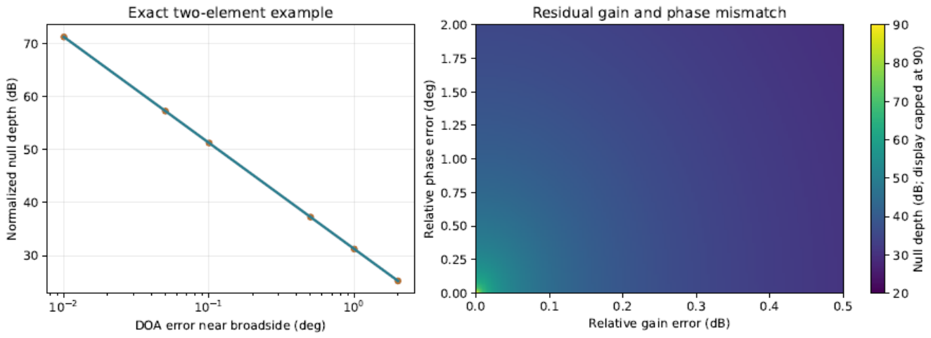
For an actual broadband array, the deepest null, the shallowest suppression over the allowed angular range, and the worst in-band frequency should be recorded separately. If a null approaches a satellite direction, the reduction in may also weaken a critical attitude direction; deepening the null need not improve attitude estimation. With multiple interference sources, the relevant quantity is the rank of the true interference subspace, not merely the number of physical transmitters. For blind covariance methods, accuracy requirements should be stated in terms of subspace estimation and tracking errors. The explicit angular tolerance of this example cannot be transferred directly to those algorithms.
7. Numerical Experiments
The experiments address three distinct sources of error. The first set uses known interference statistics to examine how the retained subspace and its coordinate representation affect attitude information. The second learns the processor from finite records and examines direction errors, residual covariance, and satellite geometry. The third isolates calibration bias using idealized observations in which the satellites have already been separated. These sets serve different diagnostic purposes; their results do not form a single performance curve for one receiver.
7.1. Array Geometry, Observation Statistics, and Evaluation
The four elements occupy the vertices of a square with side length , at , , , and . The carrier frequency is . The navigation frame uses east, north, and up coordinates, with satellite azimuth measured eastward from north. The line-of-sight vector is
For the twelve-satellite configuration, azimuths begin at zero and increase in steps. The corresponding elevations, in degrees, are 78, 25, 40, 55, 30, 65, 35, 50, 22, 60, 42, and 28. The dispersed six-satellite configuration selects satellites 1, 3, 5, 7, 9, and 11. In the clustered six-satellite configuration, the azimuths are 35, 42, 49, 56, 63, and , and the elevations are 55, 58, 61, 64, 67, and . Both six-satellite configurations use the same waveforms, per-satellite energy, and noise, isolating the effect of angular distribution. Comparisons between twelve and six satellites also involve a change in total useful signal energy.
The first two sets use 32 or 16 uniformly spaced frequency samples over . The test waveforms are obtained by QR orthogonalization of quadrature phase-shift keying (QPSK) sequences generated with fixed random seeds. They are known to the estimator; code delays and carrier frequency offsets are not estimated jointly. Stacking the observations by frequency gives
Here is the test-waveform response before channel effects are applied. Under nominal channels, each column has unit energy. The generated signals have , with phases uniformly spaced between 0.17 and 2.9 radians, while each satellite’s complex amplitude remains unknown to the estimator. The thermal-noise standard deviation is . Total interference energy per block is 45 dB above the block energy of one satellite. The true attitude has rotation vector , and every optimization starts at the identity rotation. This initialization supplies a fixed coarse alignment; the experiments do not assess a global attitude search or integer-ambiguity initialization.
The third set uses idealized, separately available satellite observations at eight frequencies. Each satellite has one unknown complex amplitude across frequency, the frequency weights are , and the generated phase is radians. The true attitude is specified by mathematical ZYX Euler angles , and the noise standard deviation is 0.02. Unlike the first two sets, the per-satellite spatial response does not include the energy normalization. Since the satellites have also been separated, absolute RMSE values from this set should be compared only within the set.
Attitude, array properties, and interference statistics remain constant within each observation block in all three sets. The first set contains 1000 trials per condition, giving 13 000 fits. The second contains 200 trials for each of 29 individual conditions and three combined conditions, giving 6400 fits. The third contains 500 trials for each of three geometries and three tolerance conditions, giving 4500 fits. Every fit is retained, including those that have not converged at termination. The attitude error and its root mean square are
Angles are reported in degrees, together with the 95th error percentile (P95) and the number of errors exceeding . This threshold diagnoses the error tail; it is not a product acceptance criterion. Percentile bootstrap intervals resample independent trials. Differences between methods are evaluated by paired resampling with the same trial indices. The intervals describe Monte Carlo uncertainty under the stated generating model. They have not been adjusted for multiple comparisons and do not cover variation in unmodeled hardware conditions.
7.2. Subspace Comparisons with Known Interference Statistics
The first set takes and uses the true interference subspace and full interference-plus-noise covariance. Raw generalized least squares (Raw GLS) retains all 128 complex observations. SP applies a common spatial null at every frequency. SF removes the interference spatial mode separately at each frequency. ST transforms the full joint block to the time domain and retains its projection onto the orthogonal complement of the complete interference subspace. The complete frequency-domain representation of ST is checked separately for numerical equivalence and is not counted as another algorithm. The mean response and covariance are transformed consistently for every processor.

Table 2.
Processor definitions. Each operation is applied consistently to the mean and covariance.
| Processor | Definition |
|---|---|
| Raw GLS | Joint generalized least squares on the complete raw block, using the full interference-plus-noise covariance. This is the reference with no discarded observations. |
| SP | A common spatial null at all frequencies, removing the spatial subspace for one or two interference directions at the carrier frequency. Residual frequency-dependent interference remains in the covariance model. |
| SF | Removal of the interference spatial subspace present at each frequency, independently and without mixing frequencies. |
| ST | Transformation of the complete block into the time domain, retaining observations in the orthogonal complement of the full space–time interference subspace. |
| SF-full | The same complete joint subspace as ST, expressed in frequency coordinates. This checks representation equivalence and is not counted as another Monte Carlo method. |
The narrowband interferer occupies one frequency sample. The coherent broadband interferer consists of one coherent mode across all frequencies. Both arrive from body-frame azimuth and elevation . In the independent split-band case, the upper and lower half-bands arrive from and , respectively, with independent coefficients at each frequency. The joint interference ranks in these three cases are 1, 1, and 32. For narrowband interference, both SF and ST retain 127 dimensions. For coherent broadband interference, SF retains 96 dimensions and ST retains 127. For independent split-band interference, both retain 96. SP retains 96, 96, and 64 dimensions, respectively. The comparison therefore concerns specific retained subspaces; the results cannot be attributed to the labels “time domain” and “frequency domain” alone.
All methods share the raw observation within a trial, and thermal-noise draws are also paired across the ideal-reference scenarios. The random seed is 20261114. Table 3 reports the clean baseline and all four processors in each interference scenario. Bootstrap intervals may differ slightly even when point estimates coincide, because the resamples differ.
Figure 4.
Attitude estimation with known interference statistics. Error bars show RMSE intervals from 2000 bootstrap resamples; black dots denote the local CRB expressed as an angular scale, and dashed lines mark the interference-free baseline.
Figure 4.
Attitude estimation with known interference statistics. Error bars show RMSE intervals from 2000 bootstrap resamples; black dots denote the local CRB expressed as an angular scale, and dashed lines mark the interference-free baseline.
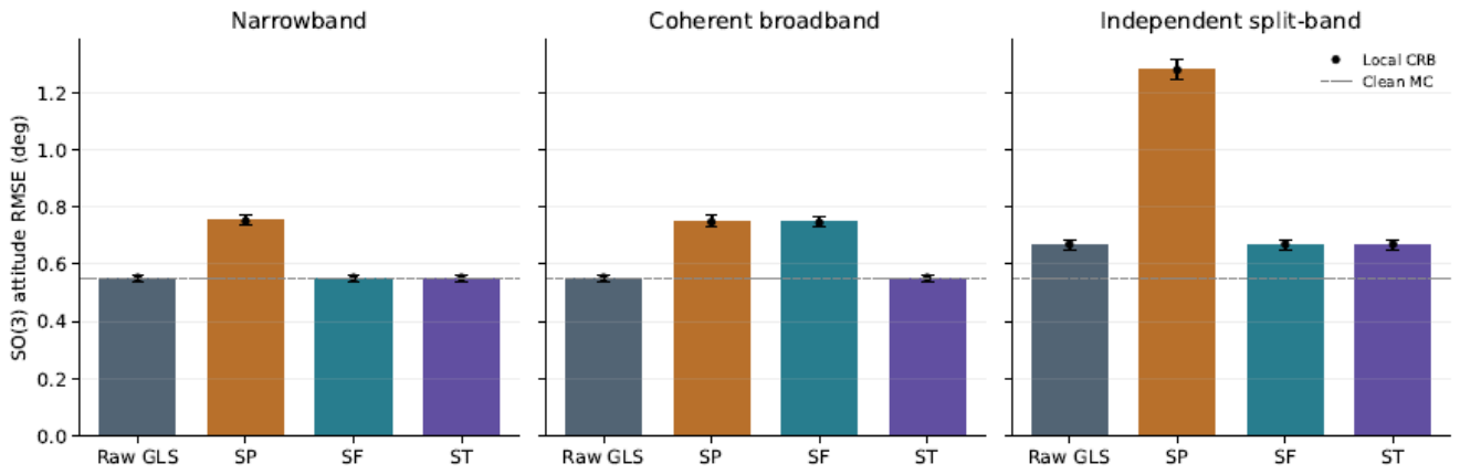
The interference-free baseline has an RMSE of 0.5482°, compared with a local CRB scale of 0.5510°. Under narrowband interference, both SF and ST give 0.5509°. Under coherent broadband interference, frequency-by-frequency SF gives 0.7496°, whereas complete ST gives 0.5493°. Under independent split-band interference, both give 0.6672°. These results agree with the subspace analysis: separate removal at each frequency can discard attitude information that a processor exploiting cross-frequency coherence would retain, whereas an invertible change of coordinates leaves statistical information unchanged. The Raw GLS RMSEs are 0.5509°, 0.5493°, and 0.6672° in the three cases, close here to those of complete-subspace processing.
The relative difference between the analytical response derivative and a centered finite difference is . Information matrices computed from complete time- and frequency-domain representations differ by no more than in relative terms. All 13 000 fits converge, and none has an error exceeding . An empirical Monte Carlo RMSE slightly below the local CRB scale does not violate the information bound: the former fluctuates with the finite trial sample, while the latter is a covariance benchmark under a local unbiased approximation.
Figure 5.
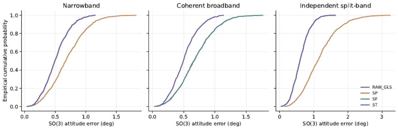
Empirical cumulative distributions of total attitude error. ST and SF coincide in the narrowband and independent split-band cases because they retain the same subspace.
Figure 5.
Empirical cumulative distributions of total attitude error. ST and SF coincide in the narrowband and independent split-band cases because they retain the same subspace.
The total rotation error does not show how roll, pitch, and yaw are affected separately. Table 4 uses extrinsic xyz Euler angles with
Yaw here is a mathematical rotation about the positive ENU z axis, not a compass heading measured eastward from north. The component errors are distinct from the total rotation angle on . Body-frame small-angle errors, component biases, and trial-level records are also retained by the program; these measures cannot be interchanged without a coordinate convention.
Figure 6.
Axis-wise RMSE in roll, pitch, and yaw, using the convention of Table 4.
Figure 6.
Axis-wise RMSE in roll, pitch, and yaw, using the convention of Table 4.
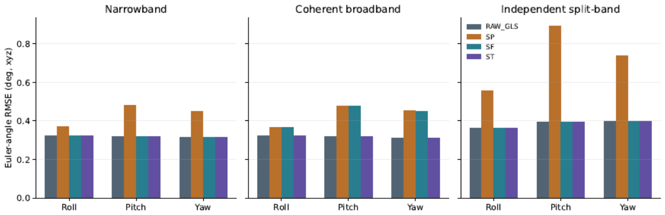
Noiseless consistency checks recover the generating attitude from the same coarse initialization. None of the projection information matrices exceeds the Raw GLS reference retaining the full observation. Biases, maximum errors, and paired-difference intervals for each method are included in the saved results. Additional losses from a common spatial null can reflect both discarded attitude directions and residual interference due to frequency-dependent responses; the name of the processing domain does not explain them.
7.3. Finite Training, Direction Errors, and Residual Statistics
The second set uses 64-dimensional observations and one coherent broadband interference mode, whose order is specified in advance as one. Each trial generates independent training data, a 256-snapshot validation set, and a test observation. Training sizes are 32, 128, and 512; shorter sets are prefixes of the same 512-snapshot record. By default, training and validation include satellite signals , with . Removing the sample mean therefore does not remove their power. The estimator receives these records, but neither the true attitude nor the true residual covariance. The random-amplitude model tests contamination of the training data; a snapshot is not assigned a millisecond duration in a physical receiver.
SP extracts the dominant eigenvector from the spatial sample covariance aggregated over frequency. SF extracts it separately at each frequency, and ST extracts it from the complete joint block in the time domain. None of these three processors requires an explicit direction estimate. SP and SF retain 48 complex outputs, whereas ST retains 63. ST is a joint-block projection in this experiment, not a causal finite impulse response (FIR) implementation with a specified tap count and an equal computational budget. An independent validation window provides the output sample covariance , and the estimator uses
Because includes the power of varying satellite signals, it differs from the true interference-plus-noise covariance of the test observation. The 5% shrinkage coefficient is not tuned to the results. Diagonal shrinkage also depends on the output basis and generally does not satisfy . The equivalence of complete time–frequency representations therefore does not extend unconditionally to this empirical procedure. The following results compare fixed implementations and reflect the combined effects of output dimension, subspace estimation, and covariance approximation.
Table 5.
Finite-sample results with 128 training snapshots. Intervals use 1000 bootstrap resamples. Suppression is the median reduction in total interference energy across trials.
Table 5.
Finite-sample results with 128 training snapshots. Intervals use 1000 bootstrap resamples. Suppression is the median reduction in total interference energy across trials.
| Method | Complex outputs | RMSE (°) | 95% interval (°) | Suppression (dB) |
|---|---|---|---|---|
| SP | 48 | 0.8165 | [0.7669,0.8667] | 63.49 |
| SF | 48 | 0.7930 | [0.7482,0.8421] | 56.82 |
| ST | 63 | 0.6117 | [0.5776,0.6487] | 55.58 |
Table 6 gives the complete results at all training sizes. P95, residual interference-to-signal ratio, null depth, and RMSE refer to the same trials. A deeper null need not make every error statistic decrease. The training and measurement trials use random seed 2026111402.
Increasing the SF training size from 32 to 512 raises median interference suppression from 50.61 to 62.84 dB, but the corresponding attitude RMSEs are 0.7881° and 0.7908°. Under these conditions, residual statistics and the retained geometry already limit attitude estimation; a deeper null does not imply a further improvement in accuracy. Removing the varying satellite component from training and validation gives an RMSE of 0.7708° for SF with 128 snapshots. This idealized case is kept separate from the default training assumption.
An explicit direction estimate is also obtained from the dominant eigenvector of the spatial covariance. A search on a grid over the upper hemisphere supplies the initial direction, which is refined by nonlinear fitting of the array response with the common complex amplitude eliminated. The upper-hemisphere prior resolves the above–below mirror ambiguity of a planar array; initialization does not use the true direction. The angular direction RMSEs for 32, 128, and 512 snapshots are 0.0325°, 0.0155°, and 0.0077°, respectively. Their attitude RMSEs are 0.8106°, 0.8122°, and 0.7981°. These values depend on the single interference mode, ideal calibration, and specified signal, interference, and noise levels. They are not general direction-estimation accuracies.
The coarse direction search covers azimuths from to and elevations from to , both in steps over the upper hemisphere. Table 7 reports azimuth, elevation, and unit-direction angular errors separately so that these distinct measures are not conflated.
To isolate the effect of direction bias, the true interference is held fixed while the design azimuth is offset by 0, 0.1, 0.5, 1, or ; the design elevation remains correct. This prescribed-bias sweep is distinct from the direction-estimation errors just reported. Both attitude estimators use the same actual processing matrix: one uses (73), and the other whitens with thermal noise alone.
Table 8.
Prescribed direction bias and treatment of residual covariance. RMSEs are in degrees. The zero-bias row represents an ideal numerical limit; the residual is zero to numerical precision.
Table 8.
Prescribed direction bias and treatment of residual covariance. RMSEs are in degrees. The zero-bias row represents an ideal numerical limit; the residual is zero to numerical precision.
| Azimuth bias (°) |
Suppression (dB) |
Residual J/S (dB) |
Estimated covariance |
Thermal only |
|---|---|---|---|---|
| 0 | zero residual | zero residual | 0.7921 | 0.7213 |
| 0.1 | 52.03 | -5.73 | 0.8178 | 1.9549 |
| 0.5 | 38.05 | 8.25 | 0.7881 | 10.2274 |
| 1 | 32.03 | 14.28 | 0.7895 | 20.7715 |
| 2 | 26.01 | 20.31 | 0.8051 | 54.9982 |
At a azimuth bias, total interference-energy suppression is 38.05 dB, and the residual interference-to-signal ratio is 8.25 dB. Using thermal noise alone gives an RMSE of 10.2274°, compared with 0.7881° when residual covariance is estimated. The latter result exploits the low-rank correlation of the residual interference. It does not make direction bias immaterial and cannot be extrapolated to multiple sources, nonstationary records, or saturation.
7.4. Joint Effects of Satellite Geometry and Channel Residuals
For SF with 128 training snapshots, the RMSEs for twelve dispersed, six dispersed, and six clustered satellites are 0.7930°, 1.7178°, and 15.8855°, respectively. The corresponding interference-free, uncompressed observations give 0.5560°, 0.8062°, and 2.7710°. In the clustered case, 139 of 200 errors exceed , and one fit reaches the iteration limit. With weak geometry, a local information bound or an average restricted to successful fits would therefore conceal much of the error tail.
Figure 7.
Attitude sensitivity with finite records. The left panel compares treatments of residual covariance, the middle panel varies the number of training snapshots, and the right panel compares satellite counts and angular distributions. Each comparison uses the fixed statistical conditions of this experiment set.
Figure 7.
Attitude sensitivity with finite records. The left panel compares treatments of residual covariance, the middle panel varies the number of training snapshots, and the right panel compares satellite counts and angular distributions. Each comparison uses the fixed statistical conditions of this experiment set.
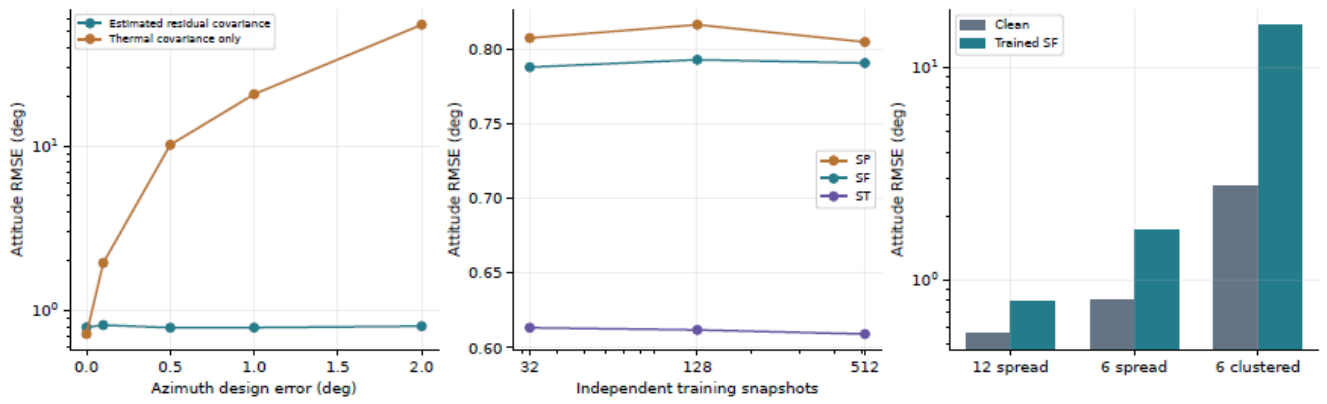
Table 9 places the clean full-observation results beside those from finite-training SF and the nominal smallest information eigenvalue. This eigenvalue is computed with the estimator’s and cannot be reinterpreted as a strict CRB for the independent test errors.
Figure 8.
Total interference-energy suppression by the implemented operators. The ideal zero-direction-error point lies outside the plotting range; its numerically zero residual is not a hardware specification.
Figure 8.
Total interference-energy suppression by the implemented operators. The ideal zero-direction-error point lies outside the plotting range; its numerically zero residual is not a hardware specification.
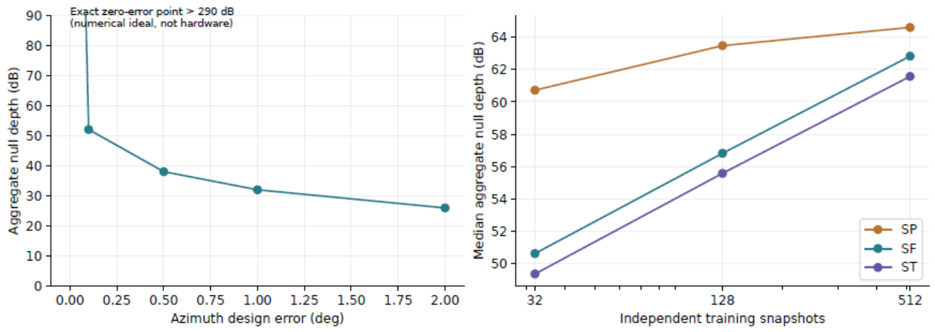
Across the 5800 fits in the separate finite-training conditions, 23 terminate without convergence and 675 exceed ; all are retained. These totals cover 29 conditions, including thermal-noise-only whitening, and should not be attributed solely to the default SF configuration in the table. Trial records are in results/producttrials.csv; biases, maxima, and RMSE intervals are in results/productsummary.json.
The combined-error trials introduce channel residuals with maximum magnitudes of 0.3 dB in gain, in phase, and 3 ns in differential group delay. These errors are fixed within each block and act on satellite and interference signals in the training, validation, and test records. Noise is added after the channel response. Signal generation uses the true , whereas fitting assumes the nominal while retaining the processing matrix actually learned from the data. The 45 dB ratio is defined using nominal energies before channel effects. Actual input energies, interference suppression, and retained satellite fractions are recalculated after the channel effects, and the corresponding power balance is satisfied in every trial.
Table 10.
Joint effects of finite training, geometry, and assumed channel tolerances. These are simulated results, not measured product specifications.
Table 10.
Joint effects of finite training, geometry, and assumed channel tolerances. These are simulated results, not measured product specifications.
| Geometry | Baseline RMSE |
Combined RMSE |
P95 (deg) | Suppression (dB) |
Count |
|---|---|---|---|---|---|
| 12 dispersed | 0.7930 | 0.9389 | 1.5440 | 56.82 | 0 |
| 6 dispersed | 1.7178 | 1.9928 | 3.6694 | 59.84 | 4 |
| 6 clustered | 15.8855 | 16.8716 | 36.7028 | 62.48 | 132 |
Each geometry uses 200 trials; the nonconvergence counts are 0, 0, and 4, respectively. Large-error outcomes motivate a separate attitude-validity criterion. Until such a criterion is defined, removing these outcomes and reporting only the remainder would conceal the failure tail. Nor can distinct error sources be added using a universal angular scale factor.
The combined-error trials and ideal-channel baseline are paired using the same random seed and sampling order. Table 11 reports the combined-condition RMSE minus the baseline RMSE, with an interval for this difference.
For both dispersed configurations, the difference intervals lie above zero. In the clustered configuration, the point estimates differ but the paired interval crosses zero, so these trials do not establish further degradation caused by the combined residuals. The stronger finding is the severe error tail under both conditions. With combined residuals, P95 is 36.7028°, 132 of 200 errors exceed , and four fits do not converge; all are included in the RMSE. Median interference suppression nevertheless reaches 62.48 dB. A deep null is thus compatible with unreliable attitude estimation.
7.4.1. Isolating Calibration Errors and Scanning Their Components
The calibration experiment uses a single interferer at body-frame azimuth and elevation . At each frequency, the exact reference-regression ratios and operator are
In this experiment, denotes the single-frequency test-waveform response before channel errors. The true satellite mean is and the fitted mean is , both using the same actual . Thermal noise has covariance after the channels and before regression, and after regression; the latter is used for whitening. Exact regression ratios isolate channel-model mismatch. Their use here does not imply that finite training recovers those ratios exactly.
The single-error scans use gains of , phase amplitudes of , and differential group delays of . The fixed gain, phase, and delay profiles are specified in Appendix A; each is normalized to its maximum absolute residual. The noise standard deviation is 0.02, and the information matrix eliminates the unknown complex amplitude of each satellite.
Table 12.
Geometric information and local error bounds under ideal calibration. The final column is not a measured product accuracy.
Table 12.
Geometric information and local error bounds under ideal calibration. The final column is not a measured product accuracy.
| Geometry | Smallest eigenvalue |
Condition number |
Local CRB (deg) |
|---|---|---|---|
| 12 dispersed | 109133.36 | 2.27 | 0.2477 |
| 6 dispersed | 36559.52 | 3.30 | 0.3947 |
| 6 clustered | 2061.46 | 139.10 | 1.2877 |
The third set separates calibration bias from finite training by assuming that reference-channel regression recovers the true interference channel ratios exactly, with whitening by the corresponding thermal-noise covariance. Interference is removed under this assumption, while attitude fitting still uses the nominal channel response. Fixed tolerances follow the channel-error profiles specified in advance. For random bounded tolerances, each non-reference channel is sampled uniformly over , , and for gain, phase, and differential group delay, respectively; the reference-channel errors are zero. Errors remain fixed during a trial. Repeated trials therefore represent different calibration states, not sample-to-sample jitter. Group delay multiplies only the frequency offset , since the phase at the carrier has already been calibrated separately.
Table 13.
Sensitivity to calibration tolerances with idealized separated-satellite observations. Angles are in degrees. Intervals for random-tolerance RMSE use 10 000 resamples of the 500 retained trial records.
Table 13.
Sensitivity to calibration tolerances with idealized separated-satellite observations. Angles are in degrees. Intervals for random-tolerance RMSE use 10 000 resamples of the 500 retained trial records.
| Geometry | Ideal RMSE |
Fixed RMSE |
Random RMSE |
Random RMSE 95% interval |
|---|---|---|---|---|
| 12 dispersed | 0.2453 | 0.3732 | 0.4459 | [0.4314,0.4601] |
| 6 dispersed | 0.3825 | 0.4836 | 0.5368 | [0.5154,0.5584] |
| 6 clustered | 1.2382 | 1.3844 | 1.7188 | [1.6251,1.8135] |
Table 14 retains P95 for every condition. The random-tolerance intervals in the preceding table quantify Monte Carlo uncertainty in RMSE, which is a different quantity. Conditions share the four-channel thermal-noise draw before regression; the seed is 2026111407.
Under ideal calibration, the smallest local information eigenvalues for the dispersed and clustered six-satellite configurations are 36559.52 and 2061.46 rad−2, with condition numbers of 3.30 and 139.10. Their RMSEs are 0.3825° and 1.2382°. An equal satellite count therefore does not provide equal attitude constraints. A fixed 0.3 dB gain-error profile produces a deterministic attitude bias of 0.15245° with twelve dispersed satellites and 0.84935° with six clustered satellites. Fixed phase errors need not be amplified by the same factor: their effect depends on their projection onto the least informative attitude direction.
Table 15.
Deterministic attitude bias from one calibration error at a time, in degrees.
| Geometry | 0.3 dB gain | phase | 3 ns delay |
|---|---|---|---|
| 12 dispersed | 0.15245 | 0.26897 | 0.00075 |
| 6 dispersed | 0.08900 | 0.31457 | 0.00069 |
| 6 clustered | 0.84935 | 0.19691 | 0.01672 |
Figure 9.
Deterministic attitude bias in separate sweeps of gain, phase, and differential group-delay errors. Only one error source varies in each panel; the others are zero.
Figure 9.
Deterministic attitude bias in separate sweeps of gain, phase, and differential group-delay errors. Only one error source varies in each panel; the others are zero.
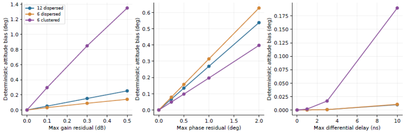
Over a symmetric band, group-delay residuals can cancel to first order once the carrier phase has been calibrated. Spectral asymmetry or the removal of frequency samples can break this cancellation. A separate test applies stale weights to changed true channels. Sweeps of 0.3 dB gain error, phase error, and 3 ns delay error give interference suppression of 34.55, 43.99, and 42.80 dB, respectively. These are stale-weight results and must not be added to the attitude-error table, which assumes accurately updated regression ratios.
Here and are the old nominal regression and whitening operators. Power is summed across frequency before suppression is calculated. Orthonormal rows exclude an apparent improvement obtained merely by scaling down the weights.
Table 16.
Interference suppression with stale weights, for fixed single-error profiles.
| Assumed residual | Normalized suppression (dB) |
|---|---|
| 0.3 dB gain residual | 34.55 |
| phase residual | 43.99 |
| 3 ns differential group delay | 42.80 |
These values apply to the stated residual profiles and arrival direction, not to a universal lower bound for errors of the same magnitude. The attitude tables use updated exact reference ratios, whereas this table uses stale weights; the two effects must not be added. All 4500 noisy calibration fits converge, including two attitude errors exceeding ; both are retained. The true is supplied only in a separate noiseless consistency check defining ideal calibration, not to the estimators in the tolerance trials.
The experiments identify mechanisms within controlled statistical models. The attitude-block chain in this section does not include measured antenna patterns, mutual coupling and polarization, clock and thermal drift, fixed-point quantization, analog-to-digital converter (ADC) saturation, automatic gain control (AGC) transients, dynamic causal filtering, or actual code correlation. Section 10 separately evaluates sampled RF and actual code correlation, without treating those navigation outputs as attitude-error measurements. In particular, the 45 dB block-energy ratio is not an equivalent validation of a 95 dB RF-input condition. Product accuracy requires measured responses and training timing to be inserted into the same observation model and the resulting estimates to be compared with an independent attitude reference.
The 128-snapshot SF case with twelve dispersed satellites appears in both the training and geometry scans. The records are identical; paired reanalysis uses one copy, so duplicate presentation supplies no additional independent evidence.
8. An Independent Experiment on Frequency-Dependent Channel-Phase Mismatch
The preceding information analysis describes how observation noise propagates into attitude when the model is correct. Another error persists under repeated measurement: processing changes the relative phases of the channels, while the estimator continues to use an ideal channel response. This section isolates that mechanism by comparing a matched model, a mismatched model, and a first-order bias prediction on the same observations. Deterministic calibration bias is kept separate from the statistical comparison of spatial, space–time, and space–frequency algorithms.
The experiment uses the four-element half-wavelength square and the dispersed twelve-satellite geometry, with eight equally spaced frequencies spanning about the carrier. This band differs from the band used in the preceding combined-calibration experiment. Each experiment uses its stated frequencies; their numerical results should not be interchanged without checking the conditions. Satellite lines of sight retain the east–north–up (ENU) convention, with azimuth a measured eastward from north:
The true attitude is defined by , with yaw , pitch , and roll . Yaw here is the mathematical Euler rotation about the positive ENU z axis, not a compass heading measured eastward from north. Each satellite has one unknown common complex amplitude across the eight frequencies, whose weights are all . Ideal code separation is assumed and no random noise is added, so that calibration bias can be examined alone. The reported errors are therefore deterministic attitude biases, not Monte Carlo RMSEs or measurements of a complete radio-frequency receiver chain.
Let be equally spaced. The fixed channel-phase profile is
These coefficient vectors specify only the phase profile and are unrelated to the element baselines . The normalization gives . If denotes the largest phase residual over all channels and frequencies, expressed in radians in the calculation, then
The profile contains both frequency-independent channel offsets and frequency-dependent terms. It is therefore not a test of group delay alone.
Reference-channel regression retains three outputs:
where and is the geometric response to a single interference source at body-frame azimuth and elevation . The coefficients are ratios of interference responses between each channel and the reference. In this conditional experiment, these ratios are assumed to be known exactly and are held fixed throughout the candidate-attitude search. They cancel the interference response, but the true satellite mean remains
Here is the geometric response in Equation (2). Both estimators receive exactly the same implemented . The matched model uses Equation (80); the mismatched model replaces only by . Regression cancels the interference without automatically correcting the relative channel errors that remain in the satellite response.
Use unit input noise covariance to define the fitting metric. The covariance after regression is
Although no random noise is injected in this experiment, this covariance still determines the residual weighting. It is positive definite and generally nondiagonal. A Cholesky factorization provides such that , preserving the correlation induced by the reference-channel noise. The phase-error matrix is diagonal and unitary, so it does not change the white-noise covariance before regression.
Let stack the whitened, unit-amplitude responses of a candidate model over frequency, and let stack the whitened observations. These symbols distinguish the whitened quantities from the raw joint responses. Eliminating the common complex amplitude at every candidate attitude gives
Every fit starts from the identity attitude; the true attitude is not used for initialization. The total error is , while componentwise Euler-angle differences follow the stated ZYX convention.
Table 17.
Deterministic attitude bias caused by unmodeled channel phase. All values are in degrees; the last three columns are differences in ZYX yaw, pitch, and roll.
Table 17.
Deterministic attitude bias caused by unmodeled channel phase. All values are in degrees; the last three columns are differences in ZYX yaw, pitch, and roll.
| Maximum channel phase residual |
Total attitude bias |
Yaw bias | Pitch bias | Roll bias |
|---|---|---|---|---|
| 0.25 | 0.06939 | -0.00418 | 0.06914 | -0.00492 |
| 0.50 | 0.13876 | -0.00839 | 0.13826 | -0.00986 |
| 1.00 | 0.27743 | -0.01689 | 0.27642 | -0.01981 |
| 2.00 | 0.55447 | -0.03421 | 0.55241 | -0.03998 |
Figure 10.
Attitude bias caused by ignoring frequency-dependent channel phase in the same reference-regression output. The left panel compares the full nonlinear fit, the first-order prediction, and the matched channel model; the right panel shows the Euler-angle biases. This fixed error profile projects mainly onto pitch, which does not imply that pitch is always the most vulnerable component in other arrays.
Figure 10.
Attitude bias caused by ignoring frequency-dependent channel phase in the same reference-regression output. The left panel compares the full nonlinear fit, the first-order prediction, and the matched channel model; the right panel shows the Euler-angle biases. This fixed error profile projects mainly onto pitch, which does not imply that pitch is always the most vulnerable component in other arrays.
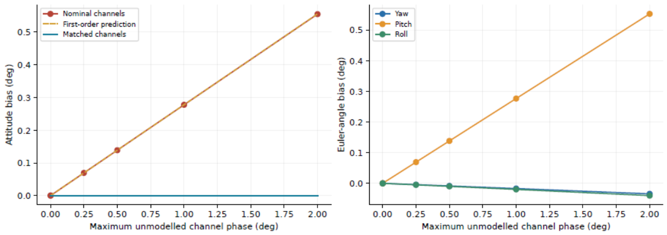
In this example, a maximum channel-phase residual of produces a total attitude bias of approximately . Increasing the residual to gives a bias of approximately . With the matched model, the noiseless attitude error is below degrees at every test point. That result checks consistency between generation and inversion of the same model; it is not an attainable engineering accuracy claim.
The trend can also be predicted from the local bias formula. Evaluate the mismatched whitened response at the true attitude and use the right-multiplicative perturbation . If the whitened true mean is , define
Stack the real and imaginary parts of and , multiplied by , over satellites to form B and . The first-order prediction is then
This is Equation (59) specialized to ideally separated satellite observations. It retains the requirements of small mismatch, local full rank, and a common solution branch. At the small-error test point of , the relative difference between the first-order prediction and the right-multiplicative rotation-error vector from the full nonlinear fit is . The analytic attitude Jacobian agrees with a central finite difference to a relative error of . Together, these checks connect the tabulated biases to the specified response mismatch, attitude sensitivity, and numerical solution.
Regression-coefficient estimation error, stochastic thermal drift, and radio-frequency nonlinearities under strong interference are not simulated in this experiment. The result shows why correcting one common phase per satellite is insufficient to ensure a consistent attitude model. What must be retained and calibrated is the relative phase structure across channels and frequencies after processing. Compensation should update the candidate mean and noise statistics together, with an explicit association between the processing coefficients and the frequency-calibration version.
9. Implementation and Product Validation of the Attitude Branch
9.1. Recorded Data and Processing Parameters
Connecting the observation model to a receiver first requires an unambiguous definition of the data supplied to the attitude branch. A virtual gyroscope needs complex responses that remain comparable across elements, together with the conditions under which those responses were formed. Its input cannot consist solely of a scalar with a free common complex amplitude. Sufficient independent spatial or joint space–time dimensions must be retained, and the processing coefficients, frequency coordinates, and measurement epoch must be available with the data.
For reference-channel regression, the action of the regression at each frequency or within each temporal kernel can be included directly in the candidate response, while retaining correlations introduced by reference-channel noise. A regression containing second-order temporal moments requires its full finite-window action; an instantaneous matrix is not an adequate substitute. Frequency-wise processing requires the effective outputs and relative phase references at every frequency. Multitap space–time processing requires the taps, readout window, and actual temporal support. A change in processing structure calls for a new check of the response model rather than continued use of the previous instantaneous model.
9.2. Quantization and Front-End Linearity
Let denote the actual weight-quantization error. For one interference response, the spectral norm gives
Word length, scaling, and saturation rules therefore constrain the realized null. There is no universal null depth determined by bit count alone, independently of the weight scale and input response. The real and imaginary quantization steps, accumulator width, rounding rule, weight normalization, and overflow behavior must be recorded. Phase-measurement resolution and weight resolution are also different specifications. When the estimation model uses the actual quantized operator, quantization still affects the null and retained information, but the difference between ideal and implemented weights must not also be counted as an unknown operator bias.
A linear error budget presupposes a linear analog front end. If strong interference drives the low-noise amplifier, mixer, or analog-to-digital converter (ADC) into a nonlinear regime, clipping, intermodulation, and unequal channel distortion change the entire observation model. Subsequent digital filtering cannot guarantee recovery of the original spatial phase. Front-end gains, the automatic gain control (AGC) state of each channel, ADC full-scale ranges, and saturation fractions should therefore be logged synchronously. Antenna phase-center, installation-baseline, mutual-coupling, pattern, and polarization residuals belong in the combined response and its attitude derivatives alongside the RF-channel calibration.
9.3. Filter Support, Update Timing, and Attitude Epoch
The timing check takes a sampling rate of , a weight-update interval of approximately , and a correlation or main tracking-loop interval of as receiver configuration inputs. Synchronized hardware logs have not yet established their actual alignment in the target product. The statistical window, completion of computation, publication of weights, and consumption of data refer to different times. Statistics that support a deep null may already be stale when the weights are used. Changes in interference direction, channel phase, and body attitude can all move the null; computation time, measurement timestamps, and filter group delay cannot be reduced to a single delay number.
Temporal support does not imply a millisecond-scale group delay. If an implementation actually uses a symmetric, linear-phase, 128-tap finite impulse response filter at , its common group delay is
At a constant rotation rate of , leaving this common pure delay uncorrected gives an attitude-epoch difference of approximately . A true timing offset of at the same rate instead gives . These are scale calculations under a pure-delay model. A division into 128 frequency bins does not, by itself, define a symmetric 128-tap linear-phase filter.
Filter duration, the correlation-integration window, the model-update interval, and transport latency must be distinguished. A common pure delay can be handled by correcting the measurement epoch; channel- or frequency-dependent complex temporal kernels generally must remain in the mean in (18). When waveform or attitude changes appreciably within the window, (61) is only a local expansion and cannot replace the full temporal integration. Motion parameters introduced to evaluate a finite-window mean should be estimated jointly or eliminated as nuisance parameters before attitude error is evaluated at the specified epoch. Angular-velocity accuracy and attitude accuracy remain separate quantities.
9.4. Model Parameters and Validation Evidence
Table 18 lists the actual quantities needed to move from the model to product evaluation. The stated sweep ranges are inputs to sensitivity experiments, not achieved product specifications. Missing entries require corresponding measurements rather than ideal values substituted in their place.
Receiver integration should follow a traceable error chain: establish the actual array response and observation conditions; compute interference leakage and retained satellite response; estimate attitude with the processed geometry and statistics; and compare synchronously against independent truth. Algorithm comparisons should use the same RF input and retain multichannel records, the actual operator, noise model, attitude epoch, and reference. Only when these conditions agree can an accuracy difference be attributed to the stated processing change.
The ideal subspace comparison, finite-training trials, and channel-error sweeps each isolate part of this chain. A receiver may also face nonstationary motion, data shared between training and measurement, time-varying coupling, and front-end dynamic-range limits. End-to-end attitude error arises from these effects together. The controlled attitude experiments do not replace measurements of the complete receiver. The following section extends the study to sampled RF, tracking, and RTK under prescribed motion, while retaining the distinction between simulated receiver behavior, independently measured attitude accuracy, and hardware performance.
10. Carrier-Reference Consistency and RTK Ambiguity Fixing
The preceding experiments evaluate attitude from coherent array records. A navigation receiver uses a different observable: the carrier phase delivered by a scalar tracking channel. To examine how the same observation conditions affect this downstream quantity, we conducted a separate set of complete synthetic receiver-chain experiments. They connect array-response consistency to carrier continuity and integer-ambiguity decisions. They do not convert the attitude RMSE of Section 7 into an RTK fixing probability. In particular, the newly executed compensated receiver uses a physical gyroscope; these runs are not a new validation of virtual-gyroscope accuracy.
10.1. From the Combined Response to a Double-Difference Residual
For the navigation output introduced in the Introduction, let denote the effective response to satellite s, relative to the reference element, and let . Here is specialized to the scalar navigation readout, including the actual channel and temporal action. With carrier phase expressed in cycles, write
Here is the L1 carrier wavelength, is the integer ambiguity on a continuous tracking arc, and is the carrier measurement error. The terms b and collect the common receiver contribution and satellite-specific clock, propagation, and modeled hardware terms, respectively. This decomposition identifies the additional response phase; it does not remove the geometric range . In the ideal interference-free reference-element bypass, the element is at the body-frame origin and . A conventional phase-locked loop (PLL) can then track physical range evolution without array-response compensation.
If the base station has no corresponding array phase, differencing rover and base observations and then satellites s and r leaves the extra contribution
A common-clock cancellation therefore does not remove a satellite-dependent array phase. On a continuous interval where ,
Both changing weights and a changing array response enter this expression. A weight switch additionally requires its finite phase change to be handled at the correct measurement time. Near a response zero, the differential expression itself becomes ill-conditioned; phase correction cannot restore the removed signal energy.
After compensation with , the additional double-difference residual is
This also explains where attitude accuracy enters. If the true attitude is locally , while all other modeled conditions are held fixed, define the row vector
For nonzero responses and sufficiently small perturbations, , with additional terms for channel, timing, and weight-model errors. Thus a shared attitude error is filtered through satellite-dependent phase sensitivities. There is no universal conversion from an attitude RMSE to an ambiguity-fixing rate: the processed geometry, nuisance biases, temporal correlation, float ambiguity covariance, and validation rules all intervene. Even a constant uncalibrated can be a fractional-cycle bias and cannot automatically be absorbed into an integer ambiguity.
10.2. Paired Receiver Experiments and Fixed Evaluation Windows
Two motion profiles were evaluated. The inherited stress profile lasts 10 s and reaches approximately and (approximately ); prescribed rotation begins at . It is a numerical stress test, not a typical civil-aircraft trajectory. The additional 6 s profile is a coordinated, constant-altitude turn at with radius . Its yaw rate is , and its centripetal acceleration is . The bank magnitude is
The body forward axis follows the velocity tangent, and the thrust direction with gravity reproduces the centripetal acceleration. These identities were checked numerically. A declared nominal initial alignment retains the inherited rotation error; time-varying true attitude is not supplied to the receiver. This profile is a stated engineering scenario, not a reconstruction of measured flight data.
Both profiles use the same four-element half-wavelength square, twelve synthetic GPS L1 C/A satellites, and nominal per-element rover and base values of 45 and 47 dB-Hz. Samples are generated individually at , with weight holds, correlation and tracking intervals, 2-bit quantization per in-phase/quadrature component after array processing, and 20 Hz positioning. A single fixed-ENU interference source has azimuth and elevation . Its 95 dB interference-to-signal ratio is measured against one unit-power satellite before array processing; it is not a residual output ratio.
For each motion profile, three receivers were compared. The clean receiver uses element 0 directly, with neither response transport nor attitude compensation. Receiver C uses the newly computed weights, denoted NEW, and no phase compensation. Receiver A uses the previously active weights, denoted OLD, together with physical-gyroscope-assisted response compensation. The physical gyroscope supplies 500 Hz packets with the inherited errors and timing model. All rover PLLs use the same gains selected before processing, , , and ; the base-station loop is unchanged.
The no-interference and interference streams share their satellite phases, motion, and counter-keyed thermal-noise realization. The two interference receivers consume identical raw array samples, with independent tracking states. Base-station sample hashes agree within each profile; the saved OLD sequences also agree between A and C, as do the saved NEW sequences. Nevertheless, A and C select different sequences. The comparison is therefore between the implemented receiver architectures, not a single-factor experiment switching compensation on the same OLD waveform. C also lacks an initial fractional array-phase calibration. Those two differences must remain part of the interpretation.
All groups use the same final ambiguity backend. The initial interval is 1 s and the ratio threshold is 3. The basic backend requires eight satellites; the inherited final estimator can use a mature seven-satellite subset only with an additional bootstrap criterion of 0.999, and includes continuity-based integer propagation, sequential integrity checks, and endpoint recovery. These rules were not relaxed for an interference condition. Receiver outputs were completed before independent truth-based scoring.
Let indicate a published FIX at a scheduled positioning epoch. We report both
Every scheduled epoch in the specified window remains in its denominator, including loss of lock and absence of a position. The 10 s profile has 200 total and 180 post-initialization epochs; the 6 s profile has 120 and 100. With no fixes during initialization, even perfect subsequent fixing gives only 90% and 83.33%, respectively, over the complete runs. The same distinction resolves an earlier 20 s record: over the whole record is after the prescribed initialization. Those earlier no-interference records used compensated A/B chains and cannot establish an uncompensated baseline; the new element-zero bypass explicitly provides that baseline.
10.3. Fixing Decisions, Integer Verification, and Position Errors
Table 19 retains both denominators and separates the receiver’s FIX flag from its conditional integer-verification label. A published FIX can be conditionally correct, detected wrong, or unverifiable under the independent phase-reference ledger. An unverifiable integer is neither credited as correct nor classified as wrong. Figure 11 displays these categories over the fixed post-initialization windows.
In the coordinated turn, the clean receiver and compensated A both publish 100/100 fixes, with three-dimensional position RMSEs of 0.970 and 1.011 cm. The new test therefore does not show an inevitable large loss in post-initialization fixing after interference is introduced. The 94 conditionally verified fixes and six unverifiable fixes in A must, however, remain distinct; the record does not certify 100 correct integer solutions.
The position errors require a further distinction. Table 20 reports all finite position outputs and the FIX subset separately. Missing positions are not assigned zero error. C in the coordinated turn provides 41 FIX outputs, 49 ratio-rejected float positions, and ten time-differenced-carrier-phase (TDCP) positions. Its all-output RMSE is 79.518 cm, whereas its FIX-subset RMSE is 3.249 cm. The latter subset has a 95th-percentile error of 4.309 cm and maximum error of 4.598 cm, but all 41 integers remain unverifiable. A small position error does not resolve an undefined integer reference.
10.4. Tracing the Rejected Epochs
Table 21 shows why a median or an average satellite count cannot explain the fixing outcomes by itself. In the coordinated turn, C and A have median reported values of 44.51 and 44.57 dB-Hz and mean locked-satellite counts of 10.965 and 10.896. Yet all 59 non-FIX epochs in C fail the ratio test. Offline evaluation of the applied weights finds satellite-dependent response-phase excursions up to approximately and a worst satellite 95th-percentile noise-normalized gain loss of approximately 15.7 dB. The response phase and weak individual channels matter even when the median tracking metric remains high. This supports response-phase inconsistency as an important mechanism, without assigning a single-factor causal fraction to compensation.
The stress profile exposes both the initial reference problem and the subsequent dynamic burden. C already fails the ratio test at four epochs from 1.0495 to 1.1995 s, before the prescribed rotation onset at 1.20017 s. Its missing initial fractional-phase calibration therefore contributes to the comparison; zero fixes cannot be attributed solely to rapid rotation or attitude-estimation error. This result is not an artifact of an offline “unknown phase” label blocking the estimator. The backend consumes numerical observations and receiver quality/continuity inputs rather than the scoring metadata. It completes integer searches at 32 post-initialization epochs, whose ratios range from 1.0039 to 1.7588, below the threshold of 3. The remaining final states comprise 147 epochs with an insufficient admissible subset and one initial-accumulation epoch. Sequential integrity isolation contributes to subset availability; these counts do not represent a physical disappearance of the twelve generated satellites.
A has only one non-FIX epoch in the stress profile, at 7.2995 s. Twelve satellites are still generated, but only seven mature satellites enter that ambiguity decision. The ratio is 11.24 and passes its threshold, whereas the bootstrap success lower bound is 0.98195375, below the inherited seven-satellite criterion of 0.999. An attempted continuation with known integers also fails its phase-residual check. The receiver retains a TDCP position rather than publishing a FIX. This rejection is a recorded integrity decision, not evidence that the full position stream has failed.
Backend identity is as important as the denominator. With the same saved observations, the basic estimator gives 174 clean and 127 compensated stress-profile fixes after initialization, whereas the final estimator gives 180 and 179. The corresponding coordinated-turn counts are 95 and 90 for the basic estimator and 100 and 100 for the final estimator. These differences arise from the inherited mature-subset and continuity/recovery logic, not from new RF observations. Comparing a basic-estimator no-interference result with a final-estimator interference result would confound the inference.
10.5. What the Receiver Experiments Establish
The experiments demonstrate that an uncompensated reference-element receiver can maintain a high fixing fraction without interference, and that the implemented compensated architecture can retain a similar fraction under the specified interference. They also identify actual rejected epochs and distinguish phase-reference bias, temporal continuity, weak channels, and backend rules. The connection to attitude theory is Equation (91): attitude uncertainty affects navigation through the phase sensitivity of the processed response. Neither fixing fraction nor position RMSE is a substitute for the three-axis attitude errors studied earlier.
The simulation still has material limits. Satellite geometry is prescribed rather than obtained from broadcast ephemerides; both records use a single random seed. The interference waveform is broadband Gaussian noise, but its spatial manifold uses the L1 center-frequency phase without a frequency-dependent propagation delay. RF clipping, ADC overload, measured multipath, temperature-dependent channel drift, and measured wideband calibration residuals are absent. The independent receiver calibration contains stated small position and channel-phase discrepancies rather than laboratory measurements. The inherited A main stream does not implement NEW-amplitude replacement. These runs consequently do not validate a 128-bin space–frequency product or a multitap space–time hardware implementation.
For the same reason, the calculated window-center null depths are not product specifications. In the stress profile their medians are 80.72 dB for the NEW branch and 106.42 dB for OLD; in the coordinated turn they are 83.17 and 108.46 dB. These numbers belong to the idealized center-frequency response and its predictive weight timing. They are not measured in-band null-depth distributions. Field validation requires synchronized per-satellite observables and lock states, actual weights and compensation values, RF operating conditions, and measured channel and attitude references. A short synthetic record with 100% published FIX does not establish a long-term 99% correct-fixing probability.
11. Discussion and Conclusions
Separating physical attitude from the conditions under which an observation is formed leads to a precise object of study: the effective tangent space of the processed complex response. Null depth measures how much interference energy is removed; attitude information measures how strongly the observations still respond to rotations about three axes. Both depend on the processing operator, but they quantify different properties. Channel gain and phase drift affect both: they can degrade an existing null and cause the predicted attitude response to depart from the true response. Increasing a noise variance does not account for this second effect, which is a mismatch in the mean.
For the conditional model with fixed statistics, Proposition 1 separates information loss into two terms. Full local information about all three attitude components is retained if and only if every effective attitude tangent lies in the retained row space. Complete space–time and space–frequency implementations satisfying (19) produce the same data and likelihood. Independent frequency constraints, covariance approximations, and training procedures can break that equivalence. Comparisons between practical algorithms should specify these structures rather than rank algorithms solely by their processing domain. Preserving the nominal gain and phase can benefit carrier measurements; attitude estimation also requires the derivatives that remain after amplitude elimination.
The finite-training experiments show that residual interference statistics matter to attitude inversion. With a design azimuth error of , two estimators using the same null and the same record produce markedly different errors when they treat residual correlation differently. This result depends on the low-rank, stationary structure of the residual interference and does not imply that front-end suppression can be omitted. Conversely, weak geometry can produce many large attitude errors even when total-energy suppression reaches approximately 62 dB. Local information then serves as a diagnostic. Performance assessment must retain all trials and report both the error tails and the solver status.
An implemented attitude branch should retain the actual processing coefficients, frequency points, and temporal support, and use the corresponding predicted response and covariance. Channel calibration should span frequency, direction, and operating state. When fixed-point weights are included in the prediction model, their principal effects are changes in the realized null and retained information, rather than an inevitable weight-model bias. Front-end saturation, intermodulation, or automatic gain control (AGC) jumps can invalidate the linear observation model; a deeper digital null alone cannot remedy them. For dynamic windows, (18) must retain the attitude history and changes in the common waveform, unless the frozen-attitude approximation can be shown to meet the required accuracy.
The receiver-chain experiment provides a complementary test of observation consistency. In the representative circular trajectory, gyro-assisted transport retains 100 published fixes in 100 post-initialization epochs, with a three-dimensional position RMSE of 1.011 cm, close to the interference-free, uncorrected reference at 0.970 cm. Of those 100 transported fixes, 94 have conditionally verified integers and six remain unverifiable. The uncorrected branch publishes 41 fixes, all with unverifiable integer labels. Its initial fractional phase and subsequent response changes are both left uncorrected, and its coefficient timing differs from the transported branch. The comparison therefore supports the role of carrier-reference consistency without assigning the entire difference to attitude error or to one compensation operation. The more severe trajectory retains 179 of 180 post-initialization fixes with transport; the remaining rejection follows the unchanged integer-reliability rule. These are controlled receiver results, not an independent measurement of virtual-gyroscope attitude accuracy.
The sensitivity results for finite complex observation blocks are not extrapolated here to product specifications. Known test waveforms, single-source training, fixed observation blocks, and assumed tolerances allow the error sources to be examined separately, but also delimit the findings. A product-level accuracy claim requires measured channel responses and residuals, actual weights and update times, interference and satellite geometry, and a synchronized comparison against an independent attitude reference. The main derivation does not depend on the particular parameter sweeps and remains applicable when these measurements become available.
GNSS attitude performance under interference must therefore be assessed through the actual observation operator, the attitude information remaining after amplitude elimination, the residual covariance, and channel-model bias. The PODA distinction between the physical and observation axes assigns each factor a place in the same model. The information-preservation criterion identifies the structural limit, while the paired numerical experiments show how it appears as direction errors, training data, geometry, and calibration change.
Data and code availability.
The accompanying material contains the generative models, fixed random seeds, all trial-level error records, figure and table scripts, and mathematical verification scripts. The paired statistical analysis and information-decomposition checks can be reproduced from the saved records and fixed seeds. All nonconverged trials and large-error records are retained.
The receiver-chain source, scenario definitions, per-epoch summaries, and mechanical consistency checks accompany the attitude code in rtkextension/. Full tracking and observation traces are supplied as a separate archive. The RF experiments use one noise seed per paired scenario; their epochs are temporally dependent, and short-run fixing fractions are not long-term reliability estimates.
Appendix A. Reproducibility and Numerical Consistency
The core proofs are given in the main text. This appendix links the equations to their implementations, specifies the residual-error profiles, and describes how to reproduce the results. After extracting the complete source package, run
python -m pip install -r requirements.txt
python run.py
By default, the ideal-reference, finite-training, combined-residual, calibration-tolerance, independent phase-bias, and null-budget experiments are rerun in a separate reproduced/ directory. Their numerical outputs are checked against the supplied published records. Debugging runs do not overwrite results/ or the manuscript. The full repetition counts are 1000, 200, and 500. Add –pdf to compile both language editions after the comparison passes. To check the supplied records, recompute paired intervals, and compile, use python run.py –reuse-results –pdf. The command python run.py –quick checks the entry point with five trials per condition in a temporary copy and does not update the published statistics or paper. The underlying simulation scripts still accept separate trial counts; any change in experimental design requires corresponding changes to the numerical claims and sample counts. Debugging runs are not substitutes for the reported study. Installation and font requirements are listed in README.txt.
| File or function | Mathematical role and outputs |
|---|---|
| run.py | Runs the attitude-block simulations, paired statistics, and mathematical checks; compares published records before optional compilation of both papers. |
| simulations/simulator.py: signal | Forms the joint response and analytical derivatives from the array, lines of sight, frequencies, and rotation vector. The right Jacobian connects rotation-vector coordinates to local perturbations; see (7). |
| make_processors | Constructs common-spatial, frequency-wise spatial, full joint space–time, and equivalent full space–frequency processors. |
| processor | Whitens stably in semi-unitary output coordinates using the SVD of a low-rank interference factor, retaining the full residual covariance. |
| projected_residual_jac | Eliminates the unknown complex amplitudes jointly and evaluates the full derivative, including its nonzero-residual term; see (26). |
| simulations/productsim.py | Retrains the interference subspace, estimates directions and downstream covariance, and evaluates satellite geometry and combined channel errors with independent training, validation, and testing. |
| simulations/calibrationproduct.py | Sweeps gain, phase, group delay, and satellite distributions; distinguishes updated reference ratios from stale weights. |
| simulations/phasebias.py | Compares correct and mismatched channel models with the same reference-regression outputs; computes deterministic attitude bias and its first-order prediction. |
| simulations/budget.py | Computes normalized two-element nulls and power budgets; these are conditional examples rather than measured product specifications. |
| simulations/geometryplot.py | Generates the geometry figure from element positions and satellite directions. |
| verifyinformation.py | Independently checks (38) and (39), a response-preserving counterexample that loses attitude information, and the complete residual derivative. |
| qa/reanalyzesaved.py | Resamples matched trial indices to preserve dependence between conditions; checks CSV/JSON consistency and the coordinate dependence of diagonal shrinkage. |
| qa/checkpublished.py | Compares independently recomputed outputs against the published records value by value, checking that reruns reproduce the data used in the paper. |
| results/summary.json | Joint-block parameters, method errors, local information bounds, paired comparisons, and numerical checks. |
| results/trialerrors.csv | Trial-level attitude errors, Euler-component errors, and solver status for each scenario and processor. |
| results/productsummary.json, results/productcombined.json | Finite training, estimated directions, prescribed direction errors, geometry, and combined-residual results; corresponding CSV files retain individual trials. |
| results/calibrationproduct.json | Geometry information, gain/phase/delay sweeps, combined tolerances, and stale-weight leakage; the corresponding CSV contains 4500 noisy fits. |
| results/phasebias.json, results/budget.json | Independent phase-error profiles, biases at each sweep point and derivative checks; two-element direction and joint gain/phase budgets. |
| figures/ | Vector PDF and PNG figures generated from the equations and data. |
| cn/paper.tex, en/paper.tex | Main files for the Chinese and English papers, each including the complete section files in its own directory. |
Numerical checks cover the attitude Jacobian, the complete variable-projection derivative, whitening, equivalence of full time- and frequency-domain representations, and the information relationship between complete raw statistics and fixed reduced observations. In the interference-free case, nonlinear RMSE is compared with the local information scale to check noise normalization and angular units. The independent phase-bias experiment also compares a small-perturbation prediction with nonlinear fitting. Successful solver termination does not establish that all engineering conditions have been validated.
Internal provenance for the array layout and observation conventions is recorded with the code, without treating those materials as published references. The attitude-block records remain separate from the new receiver-chain records in Section 10 and from earlier archived receiver results. Provenance, execution records, content correspondence, and file checksums are retained in qa/.
The fixed profiles for the combined tolerances use . The unnormalized gain, phase, and differential-delay profiles are
The first two profiles are normalized by their maximum absolute values over the channels and frequencies used, then multiplied by 0.3 dB and , respectively; t is multiplied by 3 ns. All three residuals are zero in the reference channel. These profiles are fixed in advance, not inferred from a desired attitude error. Both frequency resolutions use the same band and analytical profiles. The phase caused by group delay varies linearly with frequency offset.
Random seeds for the ideal-reference, finite-training, and tolerance experiments are stored in their result JSON files. Methods share the relevant random inputs within each trial. The number of fits is therefore not the number of independent observations, and duplicate labels for the same condition provide no additional statistical evidence. In the formal data, the finite-training SF condition with 128 snapshots and twelve dispersed satellites appears in both the training sweep and the geometry sweep. The two records are identical; paired analysis uses only one copy.
The information decomposition is checked independently with 100 random positive-definite covariances and linear processors. Direct evaluation and the two-term decomposition agree to a relative error below . In a constructed example that retains the nominal response while removing the effective attitude tangent vectors, the original information eigenvalues are 0.5, 2, and 4.5, whereas the processed information norm falls to floating-point roundoff. In a separate example with a nonzero residual, the full variable-projection derivative agrees with a centered finite difference to a relative error of approximately . Omitting the second term of (26) raises the error to approximately 15.05%. These checks test the algebra and its implementation; they do not replace the information-preservation proof or constitute a hardware experiment.
Appendix A.1. Reproducing the Receiver-Chain Extension
The receiver experiments use a separate entry point and do not replace the attitude-block trials above. The directory rtkextension/ contains the RF generator, array processor, tracking loops, navigation solver, scenario definitions, and per-epoch summaries. From the source-package root, run
python rtk_extension/run.py
python rtk_extension/run.py --scene stress
The first command runs the six-second coordinated-turn experiment; the second runs the ten-second pressure trajectory. Each launches the interference-free reference-element control and the paired interfering C and gyro-assisted A branches. New timestamped output directories preserve the supplied records. These are full-rate RF runs and require a C++17/OpenMP compiler; they are not a replay of the compact attitude data.
The summary files are rtkextension/freshcontrolsummary.json for the pressure trajectory and rtkextension/representative6s/freshcontrolsummary.json for the coordinated turn. Each retains full-run and fixed post-initialization denominators, published FIX, conditional integer labels, position errors, tracking diagnostics, and rejection counts. Companion per-epoch CSV files preserve individual outcomes. rtkextension/diagnosticexplanation.json traces the pressure-trajectory rejection to the saved receiver fields, and rtkextension/representativemechanics.json checks the circular motion and bank geometry.
Full correlation, tracking, weight, observation, and scoring records are distributed separately as SNASMORTKPairedFullResultsR120261115.zip. To replay those saved records, merge the contents of its top-level directory into rtkextension/ and follow rtkextension/READMEFIRST.txt. The source alone is sufficient for a fresh run. The continuous raw IQ stream is regenerated rather than stored. The figure and manuscript tables use the final summaries, including the coordinated-bank-specific offline response analysis; an earlier generic diagnostic log is not the source of the published values.
References
- Daneshmand, S.; Jafarnia Jahromi, A.; Broumandan, A.; Lachapelle, G. GNSS Space-Time Interference Mitigation and Attitude Determination in the Presence of Interference Signals. Sensors 2015, 15(6), 12180–12204. [Google Scholar] [CrossRef] [PubMed]
- Marathe, T.; Daneshmand, S.; Lachapelle, G. Assessment of Measurement Distortions in GNSS Antenna Array Space-Time Processing. Int. J. Antennas Propag. 2016, 2154763. [Google Scholar] [CrossRef]
- Xu, H.; Cui, X.; Li, J.; Lu, M. Distortionless Spatial Frequency Adaptive Processing in Antenna Array GNSS Receivers. Proc. 2018 Int. Tech. Meet. Inst. Navig. 2018, 260–266. [Google Scholar] [CrossRef]
- Chang, X.; Cui, X.; Lu, M.; Wen, J. Polyphase Decomposition Based Space Frequency Adaptive Processing in Antenna Array GNSS Receivers. Proc. 2020 Int. Tech. Meet. Inst. Navig. 2020, 1021–1029. [Google Scholar] [CrossRef]
- Bamberg, T.; Konovaltsev, A.; Meurer, M. Enabling RTK Positioning Under Jamming: Mitigation of Carrier-Phase Distortions Induced by Blind Spatial Filtering. NAVIGATION 2023, 70(1), navi.556. [Google Scholar] [CrossRef]
- Wang, Y. Distortion-less carrier phase tracking space-time adaptive processor based on power inversion criterion for GNSS anti-jamming receiver. IET Radar Sonar Navig. 2024, 18(5), 754–764. [Google Scholar] [CrossRef]
- Daneshmand, S.; Sokhandan, N.; Zaeri-Amirani, M.; Lachapelle, G. Precise Calibration of a GNSS Antenna Array for Adaptive Beamforming Applications. Sensors 2014, 14(6), 9669–9691. [Google Scholar] [CrossRef] [PubMed]
- Willi, D.; Meindl, M.; Xu, H.; Rothacher, M. GNSS antenna phase center variation calibration for attitude determination on short baselines. NAVIGATION 2018, 65(4), 643–654. [Google Scholar] [CrossRef]
- Meng, X. A Set-Theoretic Derivation of Physobser Axiom Irreducibility, Minimality, and Essential Uniqueness of the Physical–Observation Dual-Axis Structure. Preprints.org, 2026, manuscript 202608.1046, version 2. Preprint. Available online: https://www.preprints.org/manuscript/202608.1046/v2.
- Meng, X. The Phase Transport Fundamental Equation on the Physical–Observation Dual-Axis Structure. Preprints.org, 2026, manuscript 202608.1128, version 2. Preprint. Available online: https://www.preprints.org/manuscript/202608.1128/v2.
- Meng, X. Reconciling Strong Interference Suppression, High-Dynamic Tracking and Precise RTK Positioning Through PODA Phase Transport manuscript 202611.0204, version 1. Preprint. Preprints.org. 2026. Available online: https://www.preprints.org/manuscript/202611.0204/v1.
- Solà, J.; Deray, J.; Atchuthan, D. A micro Lie theory for state estimation in robotics. arXiv revised 2021 (v9). 2018, arXiv:1812.01537. [Google Scholar] [CrossRef]
- Golub, G. H.; Pereyra, V. The Differentiation of Pseudo-Inverses and Nonlinear Least Squares Problems Whose Variables Separate. SIAM J. Numer. Anal. 1973, 10(2), 413–432. [Google Scholar] [CrossRef]
- White, H. Maximum Likelihood Estimation of Misspecified Models. Econometrica 1982, 50(1), 1–25. [Google Scholar] [CrossRef]
- Fortunati, S.; Gini, F.; Greco, M. S.; Richmond, C. D. Performance Bounds for Parameter Estimation under Misspecified Models: Fundamental Findings and Applications. IEEE Signal Process. Mag. 2017, 34(6), 142–157. [Google Scholar] [CrossRef]
Figure 1.
Navigation and attitude observation branches. Solid and dashed paths indicate alternative access points. An implementation must specify the attitude branch and retain its operator, phase reference, and measurement epoch.
Figure 1.
Navigation and attitude observation branches. Solid and dashed paths indicate alternative access points. An implementation must specify the attitude branch and retain its operator, phase reference, and measurement epoch.
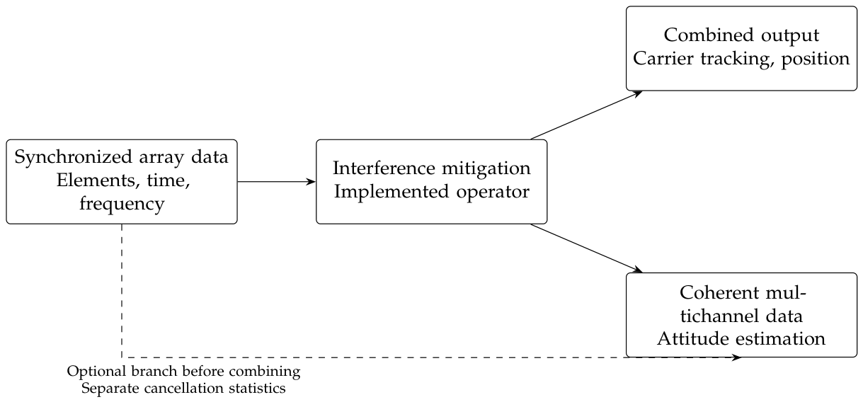
Figure 11.
Fixing and conditional verification over all scheduled epochs after 1 s. “UAV circle” denotes the coordinated-turn scenario. The gray category includes every epoch without a published FIX; no failed or missing-position epoch is removed from the denominator.
Figure 11.
Fixing and conditional verification over all scheduled epochs after 1 s. “UAV circle” denotes the coordinated-turn scenario. The gray category includes every epoch without a published FIX; no failed or missing-position epoch is removed from the denominator.
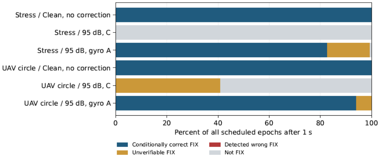
Table 1.
Null depth and power budget for the two-element example at a common processing reference plane. The last three columns are in dB; the last two give the output interference-to-signal ratio.
Table 1.
Null depth and power budget for the two-element example at a common processing reference plane. The last three columns are in dB; the last two give the output interference-to-signal ratio.
| Direction offset |
Null depth |
Input 95 No satellite loss |
Input 95 6 dB satellite loss |
|---|---|---|---|
| 0.01 | 71.24 | 23.76 | 29.76 |
| 0.05 | 57.26 | 37.74 | 43.74 |
| 0.10 | 51.24 | 43.76 | 49.76 |
| 0.50 | 37.26 | 57.74 | 63.74 |
| 1.00 | 31.24 | 63.76 | 69.76 |
| 2.00 | 25.23 | 69.77 | 75.77 |
Table 3.
Total attitude error and local information bound. All angles are in degrees; each row uses 1000 trials.
Table 3.
Total attitude error and local information bound. All angles are in degrees; each row uses 1000 trials.
| Scenario | Method | RMSE | 95% interval | P95 | CRB |
|---|---|---|---|---|---|
| No interference | Raw | 0.5482 | [0.5342,0.5616] | 0.8858 | 0.5510 |
| Narrowband | RAW GLS | 0.5509 | [0.5377,0.5637] | 0.8852 | 0.5528 |
| Narrowband | SP | 0.7544 | [0.7355,0.7743] | 1.2196 | 0.7504 |
| Narrowband | SF | 0.5509 | [0.5368,0.5642] | 0.8852 | 0.5528 |
| Narrowband | ST | 0.5509 | [0.5368,0.5642] | 0.8852 | 0.5528 |
| Coherent broadband | RAW GLS | 0.5493 | [0.5361,0.5628] | 0.8870 | 0.5529 |
| Coherent broadband | SP | 0.7509 | [0.7314,0.7700] | 1.2124 | 0.7477 |
| Coherent broadband | SF | 0.7496 | [0.7298,0.7689] | 1.2104 | 0.7454 |
| Coherent broadband | ST | 0.5493 | [0.5362,0.5623] | 0.8870 | 0.5529 |
| Independent split-band | RAW GLS | 0.6672 | [0.6511,0.6840] | 1.0631 | 0.6696 |
| Independent split-band | SP | 1.2836 | [1.2483,1.3182] | 2.1363 | 1.2792 |
| Independent split-band | SF | 0.6672 | [0.6516,0.6835] | 1.0630 | 0.6696 |
| Independent split-band | ST | 0.6672 | [0.6516,0.6835] | 1.0630 | 0.6696 |
Table 4.
Axis-wise RMSE in extrinsic xyz Euler angles, in degrees, under the stated rotation convention.
Table 4.
Axis-wise RMSE in extrinsic xyz Euler angles, in degrees, under the stated rotation convention.
| Scenario | Method | Roll | Pitch | Yaw |
|---|---|---|---|---|
| No interference | Raw | 0.3206 | 0.3173 | 0.3115 |
| Narrowband | RAW GLS | 0.3217 | 0.3173 | 0.3153 |
| Narrowband | SP | 0.3712 | 0.4805 | 0.4508 |
| Narrowband | SF | 0.3217 | 0.3173 | 0.3153 |
| Narrowband | ST | 0.3217 | 0.3173 | 0.3153 |
| Coherent broadband | RAW GLS | 0.3210 | 0.3182 | 0.3122 |
| Coherent broadband | SP | 0.3648 | 0.4786 | 0.4521 |
| Coherent broadband | SF | 0.3642 | 0.4786 | 0.4506 |
| Coherent broadband | ST | 0.3210 | 0.3182 | 0.3122 |
| Independent split-band | RAW GLS | 0.3619 | 0.3933 | 0.3990 |
| Independent split-band | SP | 0.5551 | 0.8910 | 0.7379 |
| Independent split-band | SF | 0.3619 | 0.3933 | 0.3990 |
| Independent split-band | ST | 0.3619 | 0.3933 | 0.3990 |
Table 6.
Results with the subspace learned afresh in each trial and covariance estimated from independent validation records.
Table 6.
Results with the subspace learned afresh in each trial and covariance estimated from independent validation records.
| Method | Training snapshots |
RMSE (deg) | P95 (deg) | Median suppression (dB) |
Residual J/S (dB) |
|---|---|---|---|---|---|
| SP | 32 | 0.8076 | 1.2704 | 60.73 | -14.44 |
| SP | 128 | 0.8165 | 1.3709 | 63.49 | -17.20 |
| SP | 512 | 0.8049 | 1.3385 | 64.62 | -18.33 |
| SF | 32 | 0.7881 | 1.3536 | 50.61 | -4.31 |
| SF | 128 | 0.7930 | 1.3076 | 56.82 | -10.52 |
| SF | 512 | 0.7908 | 1.3595 | 62.84 | -16.54 |
| ST | 32 | 0.6132 | 1.0189 | 49.34 | -4.27 |
| ST | 128 | 0.6117 | 0.9707 | 55.58 | -10.51 |
| ST | 512 | 0.6090 | 0.9833 | 61.58 | -16.51 |
Table 7.
Direction estimates learned from training data and the resulting attitude estimates. All angular errors are RMSEs in degrees.
Table 7.
Direction estimates learned from training data and the resulting attitude estimates. All angular errors are RMSEs in degrees.
| Training snapshots |
Azimuth RMSE |
Elevation RMSE |
Direction angle RMSE |
Suppression (dB) |
Attitude RMSE |
|---|---|---|---|---|---|
| 32 | 0.0133 | 0.0301 | 0.0325 | 68.17 | 0.8106 |
| 128 | 0.0070 | 0.0141 | 0.0155 | 73.80 | 0.8122 |
| 512 | 0.0033 | 0.0071 | 0.0077 | 80.49 | 0.7981 |
Table 9.
Effect of satellite geometry with SF and 128 training snapshots. Errors are in degrees. The smallest information eigenvalue is a nominal diagnostic in .
Table 9.
Effect of satellite geometry with SF and 128 training snapshots. Errors are in degrees. The smallest information eigenvalue is a nominal diagnostic in .
| Geometry | Clean RMSE |
SF RMSE |
P95 | Not converged |
||
|---|---|---|---|---|---|---|
| 12 dispersed | 0.5560 | 0.7930 | 1.3076 | 1104.9 | 0 | 0 |
| 6 dispersed | 0.8062 | 1.7178 | 3.1145 | 389.4 | 0 | 0 |
| 6 clustered | 2.7710 | 15.8855 | 33.0157 | 22.1 | 139 | 1 |
Table 11.
Paired effects of channel residuals. Angles are in degrees; difference intervals use 10 000 paired bootstrap resamples.
Table 11.
Paired effects of channel residuals. Angles are in degrees; difference intervals use 10 000 paired bootstrap resamples.
| Geometry | Baseline RMSE |
Combined RMSE |
Difference | 95% interval for difference |
|---|---|---|---|---|
| 12 dispersed | 0.7930 | 0.9389 | 0.1459 | [0.1058,0.1838] |
| 6 dispersed | 1.7178 | 1.9928 | 0.2750 | [0.2007,0.3461] |
| 6 clustered | 15.8855 | 16.8716 | 0.9861 | [-0.8638,2.9088] |
Table 14.
Attitude RMSE and 95th error percentile under combined tolerances, in degrees.
| Geometry | Condition | RMSE | P95 |
|---|---|---|---|
| 12 dispersed | Ideal calibration | 0.2453 | 0.4039 |
| 12 dispersed | Fixed combined tolerances | 0.3732 | 0.5888 |
| 12 dispersed | Random bounded tolerances | 0.4459 | 0.7024 |
| 6 dispersed | Ideal calibration | 0.3825 | 0.6474 |
| 6 dispersed | Fixed combined tolerances | 0.4836 | 0.8190 |
| 6 dispersed | Random bounded tolerances | 0.5368 | 0.8995 |
| 6 clustered | Ideal calibration | 1.2382 | 2.3620 |
| 6 clustered | Fixed combined tolerances | 1.3844 | 2.6442 |
| 6 clustered | Random bounded tolerances | 1.7188 | 3.1517 |
Table 18.
Parameters required for product-level attitude evaluation and the evidence available in this study.
Table 18.
Parameters required for product-level attitude evaluation and the evidence available in this study.
| Item | Actual quantities to retain | Evidence in this study |
|---|---|---|
| Interference formation | Source count, spectra, and time-varying directions; angle-error distributions for explicit DOA methods, or subspace error for blind methods | Parameter-sweep model; no corresponding product truth records |
| Null performance | Worst in-band depth at a common gain reference plane, angular tolerance, residual interference power, and satellite attenuation | Computed in every simulated trial; no measured full-band beam patterns |
| Channel gain and phase | Complex gains, group delays, mutual coupling, and calibration residuals over frequency, temperature, direction, and polarization | Stated residual sweeps; no complete product calibration matrix |
| Satellite geometry | Time-aligned lines of sight, effective per-satellite signal-to-noise ratios, blockage, and processed responses | Controlled geometry comparisons; no field ephemeris and observation records from the target product |
| Training statistics | Window length, effective independent sample count, loading and rank rules, validation window, and age of updates | Re-estimated in each trial under the stated protocol; window timing not verified by product logs |
| Digital implementation | Actual quantized weights, scaling, accumulators, overflow, and numerical precision | Weight and accumulator word lengths unspecified; the separate receiver experiment uses 2-bit I/Q samples, not a complete fixed-point hardware implementation |
| Front-end linearity | Per-channel gains, ADC ranges, AGC switching, saturation, and intermodulation records | No synchronized hardware records |
| Attitude reference | Independent reference attitude, installation transformation, timing error, and reference uncertainty | Generative truth used in simulation; no measured product-accuracy validation |
Table 19.
Fresh receiver-chain results. Clean denotes the uncompensated element-zero bypass; C and A are the receivers defined above. C/W/U gives conditionally correct, detected wrong, and unverifiable published fixes.
Table 19.
Fresh receiver-chain results. Clean denotes the uncompensated element-zero bypass; C and A are the receivers defined above. C/W/U gives conditionally correct, detected wrong, and unverifiable published fixes.
| Motion | Receiver | All epochs | Post-init. | Post-init. (%) | C/W/U |
|---|---|---|---|---|---|
| Stress | Clean | 180/200 | 180/180 | 100.00 | 180/0/0 |
| Stress | C | 0/200 | 0/180 | 0.00 | 0/0/0 |
| Stress | A | 179/200 | 179/180 | 99.44 | 149/0/30 |
| Coordinated turn | Clean | 100/120 | 100/100 | 100.00 | 100/0/0 |
| Coordinated turn | C | 41/120 | 41/100 | 41.00 | 0/0/41 |
| Coordinated turn | A | 100/120 | 100/100 | 100.00 | 94/0/6 |
Table 20.
Post-initialization three-dimensional position errors. The all-output columns include finite FIX, float, and TDCP positions. A dash denotes an empty FIX subset. Error values are in centimetres.
Table 20.
Post-initialization three-dimensional position errors. The all-output columns include finite FIX, float, and TDCP positions. A dash denotes an empty FIX subset. Error values are in centimetres.
| Motion | Receiver | Finite outputs | All RMSE | All P95 | FIX RMSE |
|---|---|---|---|---|---|
| Stress | Clean | 180/180 | 1.076 | 1.959 | 1.076 |
| Stress | C | 32/180 | 221.301 | 261.993 | — |
| Stress | A | 180/180 | 1.311 | 2.569 | 1.288 |
| Coordinated turn | Clean | 100/100 | 0.970 | 1.647 | 0.970 |
| Coordinated turn | C | 100/100 | 79.518 | 157.716 | 3.249 |
| Coordinated turn | A | 100/100 | 1.011 | 1.835 | 1.011 |
Table 21.
Post-initialization tracking diagnostics. Lock losses count per-satellite transitions from locked to unlocked in the 1 ms telemetry. Arc changes count increments in the 20 Hz ambiguity-arc labels. Medians of finite estimates do not include invalid estimates.
Table 21.
Post-initialization tracking diagnostics. Lock losses count per-satellite transitions from locked to unlocked in the 1 ms telemetry. Arc changes count increments in the 20 Hz ambiguity-arc labels. Medians of finite estimates do not include invalid estimates.
| Motion | Receiver | (dB-Hz) | Mean locked | Lock losses | Arc changes |
|---|---|---|---|---|---|
| Stress | Clean | 43.80 | 12.000 | 0 | 0 |
| Stress | C | 44.23 | 10.336 | 118 | 71 |
| Stress | A | 44.22 | 9.437 | 25 | 23 |
| Coordinated turn | Clean | 43.77 | 12.000 | 0 | 0 |
| Coordinated turn | C | 44.51 | 10.965 | 21 | 12 |
| Coordinated turn | A | 44.57 | 10.896 | 5 | 3 |
Disclaimer/Publisher’s Note: The statements, opinions and data contained in all publications are solely those of the individual author(s) and contributor(s) and not of MDPI and/or the editor(s). MDPI and/or the editor(s) disclaim responsibility for any injury to people or property resulting from any ideas, methods, instructions or products referred to in the content. |
© 2026 by the authors. Licensee MDPI, Basel, Switzerland. This article is an open access article distributed under the terms and conditions of the Creative Commons Attribution (CC BY) license (http://creativecommons.org/licenses/by/4.0/).
Copyright: This open access article is published under a Creative Commons CC BY 4.0 license, which permit the free download, distribution, and reuse, provided that the author and preprint are cited in any reuse.