

Submitted:
13 November 2026
Posted:
16 November 2026
You are already at the latest version
Abstract
Acoustic emission (AE) signals from ball screws vary with operating conditions, specimen identity, and worn state; overall intensity alone incompletely characterizes wear-related changes. Two nominally identical ball screws were tested under 36 combinations of pre-tension force, load, and speed, covering healthy states and four local wear regions. Controlled comparisons quantified healthy spectral differences and changes in overall power, band power, and spectral shape relative to healthy signals from the same specimen and condition. Matched healthy references provided standardized-difference representations for a condition-paired reference-normalized mean network, evaluated for cross-specimen transfer with matched conditions, one unseen factor, and three jointly unseen factors. Healthy spectral differences associated with speed exceeded those associated with pre-tension force or load. Overall power changed in different directions across wear regions; two regions exhibited decreased 20–400 kHz power alongside increased 115–210 kHz power under 22 and 19 conditions, respectively. Bidirectionally averaged balanced accuracies were 97.15%, 94.99%, and 92.78%. The standardized difference outperformed no-reference, mismatched-reference, and logarithmic-difference controls in the most challenging task. Joint overall- and band-power analysis characterized local wear more completely, while matched-reference standardized differences supported cross-specimen healthy/worn-state recognition in this experiment.
Keywords:
ball screw
; acoustic emission
; shaft pre-tension force
; local wear
; varying operating conditions
; healthy reference
; cross-specimen state recognition
1. Introduction
Ball screws are key transmission components in the feed systems of computer numerical control machine tools. Wear on their raceways affects motion accuracy and operational reliability. Identifying healthy and worn states from operating signals is an important part of ball screw condition monitoring. However, measured signals contain both wear-related changes and variations associated with operating conditions and individual specimens. Characterizing these variations and the differences between worn and healthy states provides a basis for state recognition.
Ball screw condition monitoring has used vibration, torque, and AE signals [1]. Lee et al. developed a ball screw fault diagnosis system using vibration signals [2]. Pandhare et al. monitored ball screw health with inertial sensors and estimated backlash-related degradation [3]. Han et al. investigated diagnostic features for preload loss in ball screw–nut assemblies and their adaptability to changing operating conditions [4]. For fault recognition in other rotating machinery, Yu et al. represented vibration signals as higher-order networks and used community clustering to identify bearing faults under different operating conditions and fluctuating speeds [5]. These studies established relationships between operating signals and mechanical states from different perspectives, providing a basis for signal feature analysis and state recognition.
To address signal distribution differences between training and testing conditions, Azamfar et al. applied deep domain adaptation to ball screw fault diagnosis [6], while Xie et al. investigated diagnostic transfer across operating conditions and measurement positions [7]. Wang et al. combined feature enhancement, multi-kernel maximum mean discrepancy, and adversarial domain adaptation for vibration-based fault recognition across rotational speeds and ball screw specimens [8]. In general domain adaptation research, Zhang et al. used attention weighting and conditional adversarial learning to reduce the influence of non-transferable features on recognition [9]. These methods learn features that can be used across different conditions. For a specific experiment, signal analysis is also needed to identify the spectral characteristics associated with operating-condition changes and wear-state changes.
AE signals reflect friction, contact, and local material deformation and have been used to monitor rotating machinery [10]. D’Emilia et al. collected vibration and AE signals from damaged ball screws under different operating parameters for defect detection and localization [11]. Angelopoulos and Kappatos compared the responses of different AE sensors to artificially induced surface wear events in steel plate degradation experiments, assessing the effectiveness of AE for surface damage detection [12]. These experiments showed that AE can provide information on changes in the condition of contacting surfaces.
AE signals are affected by both operating and measurement conditions. In rolling bearing experiments, Cockerill et al. found that the root mean square (RMS) of healthy AE signals varied markedly with speed, whereas the effect of load was weaker; different frequency bands also showed different responses [13]. Cornel et al. examined the effects of speed, lubrication, and sensor position on AE signals, showing that operating conditions and signal transmission paths affect measured responses [14]. For ball screws, Zhang et al. investigated the effect of shaft pre-stretching on the natural frequencies of a feed system through theoretical analysis and experiments [15]. Including shaft pre-tension force as a controlled factor alongside load and speed therefore helps characterize healthy signal variations under combined operating conditions and supports comparisons between healthy and worn states under matched conditions.
The way wear signals are evaluated also affects the interpretation of experimental observations. Hase et al. observed a decrease in AE level during the transition from severe to mild wear [16]. In steel contact experiments, Geng et al. found that different frequency components had different relationships with friction and wear, while overall RMS or energy combined information from these components [17]. Renhart et al. analyzed AE band responses at different speeds and operating stages [18]. Strablegg et al. combined RMS, power spectral density (PSD), and normalized PSD to describe tribological changes in lubricated contacts [19]. These results show that wear-related changes appear in overall signal intensity as well as individual frequency bands and spectral shape, and that these characteristics should be considered together.
Existing studies provide a basis for ball screw state recognition, diagnosis under varying operating conditions, and spectral analysis of friction and wear. Diagnostic studies emphasize feature extraction and recognition across conditions, whereas tribological experiments examine the relationships between frequency components and contact processes. Incorporating operating conditions, specimen differences, and local wear regions into a common experimental framework allows healthy signal differences and wear-related changes to be associated with specific conditions. It also enables comparison of how overall power and band power describe wear characteristics.
This study investigated AE signals from healthy states and local wear regions on two nominally identical ball screws under combinations of shaft pre-tension force, load, and speed. The main contributions are as follows:
(1) Controlled comparisons were performed by varying one operating factor within each specimen and comparing specimens under identical conditions. Differences in healthy AE spectral intensity and shape were quantified to characterize the signal variations associated with operating factors and individual ball screws within the tested range.
(2) Using healthy signals from the same specimen and operating condition as references, overall and band-power changes were compared across four wear regions. The magnitudes and numbers of conditions exhibiting simultaneous overall power reduction and local band-power increase were quantified. The effects of frequency-band boundaries and healthy signal segment positions on these comparisons were also analyzed.
(3) Matched healthy references were used to construct a standardized-difference representation. Healthy/worn-state recognition was evaluated in three bidirectional transfer tasks. No-reference, mismatched-reference, and logarithmic-difference controls were used to assess the roles of healthy references and standardized-difference processing.
Section 2 describes the experimental platform, wear specimens, and dataset. Section 3 analyzes healthy signal differences and wear-related spectral changes. Section 4 presents the recognition method based on healthy references and the transfer tasks. Section 5 reports recognition results, control experiments, and discussion. Section 6 presents the conclusions.
2. Test Specimens and Data Acquisition
2.1. Experimental Platform and Operating Conditions
Two SFU1605 ball screws, designated S1 and S2, were used as test specimens. Each had a nominal diameter of 16 mm, a lead of 5 mm, a total length of 480 mm, and an effective travel of 250 mm. Figure 1 shows the experimental platform and its main components. A stepper motor drove the test ball screw through a coupling. The screw was supported by bearing housings, and the worktable moved along linear guides, with limit switches at both ends of the travel. Shaft pre-tension force was measured using a JHHM-4 load cell; the measurement arrangement is shown in Figure 2a.
The AE acquisition system consisted of a sensor, a signal conditioner, and data acquisition hardware. The AE sensor was an MAE-150P with a built-in amplification module. Its output was processed by an MSS-C01 signal conditioner and transmitted to a computer through an NI data acquisition system comprising an NI-9775 input module and a cDAQ-9181 chassis. The sensor was attached to the worktable using a couplant and moved with it; its position is shown in Figure 2b. The sampling frequency was 1 MHz, and the acquired signals were expressed as voltages in V. Sensor position, coupling method, and acquisition settings were kept unchanged across operating conditions.
The operating factors were shaft pre-tension force, load, and rotational speed. Pre-tension force was set to 0, 25, 50, and 75 kgf; load to 10, 15, and 20 kg; and speed to 300, 400, and 500 r/min. A full factorial design yielded 36 operating conditions. Both ball screws were tested under all conditions. Table 1 lists the factor levels.
2.2. Healthy States and Local Wear Regions
Each ball screw had a healthy state and two local wear regions. The wear regions on S1 were designated W1 and W2, and those on S2 were designated W3 and W4. Local wear was produced by manually abrading the raceway surface with sandpaper. Figure 3 shows the surface morphology of each region.
Surface images were used to show the morphology of the wear regions, and calibrated projected dimensions were used to describe their visible extent. Because wear depth and material loss were not measured, these dimensions were not used to classify wear severity. The diagnostic task was defined as recognition of healthy and worn states. Image annotations indicated visible wear boundaries only; they were not used as damage labels or model inputs.
Under each of the 36 operating conditions, AE signals were acquired once for the healthy state and each of the two wear regions on each ball screw. Worktable motion away from the motor along the screw axis was defined as the positive direction. All signals were acquired during constant-speed worktable motion in this direction. The two ball screws provided 216 signal acquisitions: 72 healthy and 144 worn. Each complete acquisition was treated as one sample for recognition. Spectral windows selected subsequently were used only to construct model inputs and were not counted as independent specimens. Healthy signals covered a longer travel range, whereas worn signals were extracted around the corresponding local regions; their lengths and spatial coverage therefore differed.

Table 2.
Dataset composition.
| Specimen | Healthy acquisitions | Wear region | Acquisitions per wear region | Total acquisitions |
|---|---|---|---|---|
| S1 | 36 | W1、W2 | 36、36 | 108 |
| S2 | 36 | W3、W4 | 36、36 | 108 |
| Total | 72 | 4 local regions | 144 worn signals | 216 |
Each state or wear region covered 36 operating conditions, with one acquisition per condition.
3. Analysis of Healthy and Worn AE Signals across Operating Conditions and Specimens
3.1. Raw Waveforms and Spectral Analysis
Figure 4 shows the raw AE voltages at a load of 15 kg, a pre-tension force of 25 kgf, and a speed of 400 r/min. A central 100 ms segment was extracted from each healthy and worn signal of S1 and S2. All panels use the same voltage range and show the measured waveforms without filtering or amplitude normalization.
To ensure that signal segments extracted at different speeds represented the same axial length, each window spanned one quarter of a screw revolution, corresponding to an axial displacement of 1.25 mm. For a sampling frequency fs and a rotational speed n, the number of samples per window was calculated using Equation (1). Speeds of 300, 400, and 500 r/min corresponded to window durations of 50, 37.5, and 30 ms, respectively. Each window was demeaned and multiplied by a Hann window. Any remaining signal at the end of an acquisition that was shorter than one complete window was excluded from spectral calculations.
The one-sided PSD described the distribution of signal power over frequency, with units of V2/Hz. PSD was normalized by the Hann window energy [20,21]. Let u denote the demeaned voltage, w the Hann window, and U = Σw2. The one-sided spectrum coefficient αk was 1 at the direct-current and Nyquist components and 2 at all other frequency components:
To compare spectra across speeds, the 20–400 kHz range was divided into 400 equal frequency bands, each 950 Hz wide. The average PSD in each band was calculated using the integrated power in that band and the weights of the selected signal windows:
Here, Bᵦ is the bth frequency band, M is the number of signal windows included, Si(fi,j) is the PSD of window i at frequency fi,j, Δfi is the frequency spacing, and ωi is the normalized weight of that window. Repeated selection of the same window contributed according to its selection count. When a spectral instance was interpolated from adjacent signal windows, their weights incorporated the interpolation coefficients. The weights were normalized as follows:
Here, ci is the accumulated weight determined by selection counts and interpolation coefficients.
Power calculations were checked by comparing the PSD integral over the full frequency range with the mean square of the windowed signal normalized by the Hann window energy. Subsequent analyses used integrated power within specified bands to describe signal intensity and normalized PSD to compare spectral shape. The same calculations were used to analyze differences associated with operating conditions, specimens, and healthy versus worn states.
3.2. Effects of Operating Conditions and Specimen Differences on Healthy AE Signals
This section separately compares healthy signal differences associated with operating conditions and specimen identity. For operating-condition comparisons, two factors were held fixed within the same specimen while pre-tension force, load, or speed was varied. For specimen comparisons, healthy AE signals from S1 and S2 were compared under identical conditions. Two measures were used: the symmetric relative distance between amplitude spectral densities,DASD, and the total variation distance between normalized PSDs, DTV. The former reflects differences in both spectral intensity and shape, whereas the latter describes spectral shape differences. Amplitude spectral density (ASD) is the square root of PSD. Normalized PSD was defined as:
Here, S(f) is the PSD and q(f) is its normalized form. Let Sₐ and Sᵦ denote the PSDs of two signals being compared and qₐ and qᵦ their corresponding normalized PSDs. The two distances were calculated using Equation (6):
Both distances are dimensionless, with larger values indicating greater spectral differences. Distances were calculated for the operating-condition and specimen comparisons described above. Their means and sample standard deviations are summarized in Table 3. Each distance calculation between two signals counted as one comparison.
Among the operating-condition comparisons, DASD associated with speed was 0.54513 for S1 and 0.53145 for S2, exceeding the mean distances for pre-tension force and load in each specimen. The corresponding DTV was also higher than those for the other two factors, indicating that speed-related spectral differences involved both intensity and shape. Cockerill et al. likewise observed a greater effect of speed than load on healthy AE RMS in rolling bearing experiments [13]. This study extends the comparison to matched spectra from two ball screws under combinations of pre-tension force, load, and speed. For the specimen comparison, DASD and DTV between S1 and S2 under identical conditions were 0.31086 and 0.18908, respectively, exceeding the pre-tension-force and load comparison results for both specimens. Thus, even under identical operating conditions, the healthy AE signals of two nominally identical ball screws differed in spectral intensity and shape.
Figure 5 shows how healthy AE spectra varied with operating conditions. The upper and lower rows correspond to S1 and S2, respectively; the three columns compare pre-tension force, load, and speed. Each curve was averaged over combinations of the other two factors. Mean PSD curves at different pre-tension forces and loads overlapped substantially, whereas those at different speeds were more distinct, consistent with the larger speed-related spectral distances in Table 3.
Figure 6 compares the 20–400 kHz band power at different speeds. Thin gray lines connect the three speed results for each fixed combination of pre-tension force and load. The thick red line shows the mean power over the 12 combinations. Mean power increased with speed for S1. For S2, mean power was similar at 300 and 400 r/min and increased markedly at 500 r/min. The individual curves also show differences in the magnitude and direction of power changes among pre-tension-force and load combinations.
Power ratios between speeds were first calculated for each fixed pre-tension-force and load combination and then averaged over the 12 combinations. The 400/300 r/min ratios were 1.34832 and 1.28934 for S1 and S2, respectively; the 500/300 r/min ratios were 2.56299 and 2.57279; and the 500/400 r/min ratios were 1.85544 and 1.77246. These are means of individual ratios, which differ from ratios between points on the mean power curves in Figure 6.
Healthy AE differences were associated with both operating conditions and specimen identity. Within the tested factor ranges, speed comparisons produced larger spectral differences. Healthy spectra from the two nominally identical ball screws also differed in intensity and shape under identical conditions.
3.3. Spectral Changes in Worn Signals Relative to Healthy Signals
This section analyzes band-power and spectral-shape changes in AE signals from four wear regions, using healthy signals from the same ball screw under the same operating condition as the reference. W1 and W2 on S1 and W3 and W4 on S2 were each compared with their corresponding healthy signals under all 36 conditions. The log2 ratio of worn to healthy band power described power changes, while the total variation distance DTV defined in Section 3.2 described spectral shape differences. The band-power log2 ratio was defined as:
Here, PW,B and PH,B are the integrated powers of worn and healthy signals, respectively, within band B. A log2 ratio of 0 indicates equal power; positive and negative values indicate increased and decreased power in the worn signal, respectively. Values of 1 and −1 indicate that worn-signal power is twice and half the healthy-signal power, respectively.
Table 4 shows that, relative to healthy signals from the same ball screw under the same conditions, 20–400 kHz power increased under 25 conditions for W1 and 32 conditions for W3, with median power log2 ratios of 0.3738 and 0.3369, respectively. Power decreased under 35 conditions for W2 and 33 conditions for W4, with medians of −0.7997 and −0.6053. The interquartile range was entirely positive for W3 and entirely negative for W2 and W4, whereas it crossed zero for W1, indicating variation in the direction of its power change across conditions. The DTV values for the four wear regions ranged from 0.2447 to 0.2591. All regions therefore showed spectral shape differences relative to the healthy state, although the direction of band-power change was not uniform.
To examine frequency-dependent power changes, the 20–400 kHz range was divided into four equal bands, and worn-to-healthy power log2 ratios were calculated under matched conditions (Table 5). In the 20–115 kHz band, the median ratios were 0.3727 and 0.3372 for W1 and W3 and −0.8063 and −0.6133 for W2 and W4, respectively. Their directions agreed with the overall band-power changes in Table 4. In the 115–210 kHz band, all four regions had positive median ratios; power increased under 34, 23, 31, and 22 conditions, respectively. Thus, although W2 and W4 showed reduced overall power under most conditions, power increased in this band under more than half of the conditions. By comparison, median power log2 ratios in the 210–400 kHz range were closer to zero for all regions.
Figure 7 presents the comparisons through mean spectra and individual operating conditions. The left column shows the spectral distributions of healthy and worn signals, and the right column shows the distribution of overall band-power changes across conditions. Together with Table 5, the results show that wear regions differed both in the direction of power change and in its magnitude across frequency bands.
These results show that overall power reduction can coexist with a local band-power increase in some wear regions. The next section compares overall and local band-power changes within each operating condition and counts the conditions in which both changes occurred.
3.4. Relationship between Overall and Local Band-Power Changes
To examine whether overall and local band power changed in the same direction, 20–400 kHz overall power and 115–210 kHz local band power were compared under each of the 36 conditions, using healthy signals from the same specimen and condition as the reference.
Table 6 shows that simultaneous overall power reduction and local band-power increase occurred under 9, 22, 2, and 19 conditions for W1, W2, W3, and W4, respectively. Of these, reductions in overall power of at least 10% accompanied by increases in local band power of at least 10% occurred under 4, 11, 0, and 13 conditions, respectively. This combination was more frequent in W2 and W4, indicating that reduced overall power in these regions did not imply reduced power in every frequency band.
In Figure 8, each point corresponds to one operating condition, with color indicating speed. The horizontal and vertical axes show the log2 ratios of overall and local band power, respectively. Points in the upper-left quadrant represent overall power reduction with local band-power increase, and their distribution shows the magnitudes of both changes. The magnitudes varied across conditions within the same wear region. Under some conditions, both powers increased or decreased together.
When the local band was shifted to equal-width ranges of 95–190 kHz and 135–230 kHz, simultaneous overall reduction and local increase occurred under 27 and 19 conditions for W2 and under 21 and 19 conditions for W4, respectively. The phenomenon persisted after the band boundaries were changed, although its frequency varied. Overall and band power therefore describe different aspects of worn-signal changes, and overall power increases or decreases alone do not fully describe the spectral response.
3.5. Effect of Healthy Signal Segment Position on Power Comparisons
To examine whether the position of the healthy signal segment affected the comparisons in Section 3.4, the window selection for worn signals was kept unchanged. Segments containing the same number of signal windows were extracted from the corresponding healthy signal so that both covered the same axial length. Each healthy segment was shifted by one signal window to traverse all available positions. Overall and local band-power log2 ratios were calculated between the worn signal and each healthy segment.
For each operating condition, the median power log2 ratio over different healthy segments was plotted against the original comparison result (Figure 9). The dashed line indicates equality between the two results. Points above and below the line indicate that using equal-length healthy segments increased or decreased the ratio, respectively.
When summarized over the 36 conditions, median overall power log2 ratios for W1, W2, W3, and W4 changed from 0.3738, −0.7997, 0.3369, and −0.6053 to 0.4459, −0.7005, 0.4398, and −0.4610, respectively. W1 and W3 continued to show predominantly increased overall power, while W2 and W4 showed predominantly decreased power. The general directions remained consistent with the original comparisons for all four regions.
The consistency of change directions across healthy segments was also counted for each condition. For W2 and W4, 27 and 24 conditions, respectively, showed overall power reduction in at least 90% of healthy-segment comparisons. However, when the same 90% criterion was applied to simultaneous overall reduction and local increase, only 3 conditions qualified for each region; none qualified for W1 or W3. No condition in any region exhibited both changes in every healthy-segment comparison.
Changing the position of the healthy signal segment preserved the general direction of overall power changes across the four wear regions, whereas the occurrence of simultaneous overall reduction and local increase varied with segment position. The counts in Section 3.4 describe the original window selection; the present analysis shows how different positions within the healthy signal affected those comparisons.
4. State Recognition Using Healthy References and Transfer Task Definitions
4.1. Signal Preprocessing and Spectral Matrix Construction
The model used amplitude spectra of AE signals as input features. Each signal was windowed, transformed into spectra, and sampled at selected positions to construct matrices containing eight spectra, each with 384 frequency points. The input construction procedure was as follows.
Windowing followed Section 3.1: each signal window spanned one quarter of a screw revolution, corresponding to 1.25 mm of axial displacement. Each window was demeaned, multiplied by a Hann window, and transformed using the fast Fourier transform (FFT). The one-sided amplitude spectrum was scaled by 2/Nw, where Nw is the number of samples in the window. The 20–400 kHz range was retained and linearly interpolated along frequency to 384 equally spaced points. Amplitude spectra used by the model were calculated separately from the PSDs used for signal analysis in Section 3.
Let Ai denote the amplitude spectrum of signal window i. Logarithmic compression gave the spectral feature xi = ln(1 + Ai). Eight spectra were then selected according to the number of signal windows M in the acquisition. For M > 12, up to 24 starting positions were spaced uniformly along the signal. Twelve consecutive windows were taken from each starting position, and spectra at zero-based indices 0, 2, 3, 5, 6, 8, 9, and 11 were selected. These indices were determined by round(linspace(0,11,8)), which selected eight approximately uniformly spaced positions within the twelve windows. Each starting position produced an 8 × 384 spectral matrix. For 8 ≤ M ≤ 12, only one matrix was constructed. Eight positions were set across all available windows using linspace(0,M−1,8). Non-integer positions were represented by linear interpolation between the spectral features xi of adjacent windows.
Signals of different lengths were thus represented by one or more 8 × 384 spectral matrices X. Rows represented relative spatial positions, and columns represented frequency points. Healthy-reference processing, described in Section 4.2, converted these matrices into the standardized-difference inputs used by the network.
4.2. Healthy References and the Standardized Difference
To reduce healthy signal differences across operating conditions and specimens, each signal being evaluated was compared with healthy signals from the same specimen under the same operating condition. Healthy signals were converted into spectral matrices as described in Section 4.1 and used to construct a healthy template.
For a worn signal, reference matrices were taken from the corresponding healthy signal. For a healthy signal, reference matrices using signal windows that overlapped those of the evaluated input were excluded, preventing the same signal segment from being used in both the input and its reference template. If no reference matrix was available, that input–reference combination was not constructed.
Let R denote the set of available healthy reference matrices. Averaging corresponding elements across these matrices yielded the healthy template r. The same transformation was then applied to the evaluated matrix X and template r:
r = mean(R), g(u) = ln[1 + 1000 max(u, 0)]
The dimensions of X, each reference matrix in R, and r were all 8 × 384. Here, u denotes a logarithmically compressed spectral feature from Section 4.1 or the corresponding template mean. The operation max(u,0) provided numerical protection. The healthy template was averaged before applying g.
At each frequency, the standard deviation of the transformed healthy template g(r) across its eight positions was calculated as σᵣ, using a denominator of 8. These standard deviations determined the stabilizing term εᵣ:
εr = 0.10 median{σᵣ(f): σᵣ(f) > 10⁻⁸} + 0.05
If no standard deviation exceeded 10−8, the median term was set to 1. The standardized difference between the evaluated matrix and healthy template was then calculated as:
The numerator expresses the spectral change relative to the healthy template. The denominator scales the difference according to the variation of the healthy template at the corresponding frequency. The stabilizing term prevents excessively small denominators, and clipping limits values to [−8,8]. The resulting single-channel 8 × 384 standardized-difference matrix Z was used as the network input.
4.3. Network Architecture and Training
The Condition-Paired Reference-Normalized Mean Network (CP-RNM) consisted of a shared spectral encoder, mean aggregation, and a classifier. The eight standardized-difference spectra in each input matrix passed separately through the same encoder, mapping each 384-dimensional spectrum to a 48-dimensional feature vector. The eight vectors were averaged to identify the healthy or worn state associated with that matrix.
The encoder used fully connected layers with dimensions 384 → 128 → 64 → 48, with layer normalization and GELU activation at each layer. Dropout with a rate of 0.15 followed the first activation. The classifier used a 48 → 64 → 1 fully connected structure, with GELU and dropout at a rate of 0.15 in the hidden layer. A sigmoid function converted its output into a wear probability. If an acquisition contained multiple input matrices, their predicted probabilities were averaged to obtain the recognition score for the complete signal:
eᵢ = Eθ(zᵢ), eᵦ = ⅛ Σᵢ₌₁⁸ eᵢ, pᵦ = sigmoid(Cθ(eᵦ)), p = meanᵦ(pᵦ)
Here, zi is spectrum i of the input matrix; Eθ and Cθ denote the encoder and classifier, respectively; ei is the encoded feature; eᵦ is the mean of the eight feature vectors; pᵦ is the probability predicted for the matrix; and p is the recognition score for the complete signal. Figure 10 shows the architecture, with solid blue and dashed green lines indicating source- and target-domain processing, respectively.
The network was trained using binary cross-entropy loss. Healthy and worn states were labeled 0 and 1, respectively, and each input matrix inherited the state label of its acquisition:
Here, B is the number of input matrices in a training batch. Because healthy signals and different wear regions yielded different numbers of matrices, inverse-frequency sampling weights were assigned according to the matrix counts of the healthy group and each wear-region group. This prevented groups with more matrices from dominating training. Validation and testing metrics were calculated for complete acquisitions; multiple matrices from one signal were not counted as separate test samples. Table 7 lists the network and optimization settings.
For each task, available data from the training ball screw were divided into training and validation sets by operating condition, with approximately 25% of conditions used for validation. All signals from the same condition were assigned to the same set. Model parameters were selected using validation AUC during training.
The model predicted a wear probability for each complete signal. Signals with probabilities at or above the classification threshold were classified as worn; the others were classified as healthy. The threshold was determined using the validation set. Candidate thresholds were the 2nd through 98th percentiles of the validation probabilities, at one-percentile-point intervals, after duplicate values were removed. The candidate yielding the highest BACC was selected, with ties resolved by choosing the threshold closest to 0.5. Model parameters and the classification threshold were fixed during testing. Healthy signals from the target ball screw were used only to construct references as described in Section 4.2, and wear labels were used only to calculate evaluation metrics.
4.4. Transfer Task Definitions
Bidirectional transfer between S1 and S2 was used to assess recognition of healthy and worn states on another ball screw. Data used for training and validation constituted the source domain, and data from the other ball screw used for testing constituted the target domain. For S1 → S2, the model was trained and validated using S1 data. Once its parameters and classification threshold had been determined, it was tested on the healthy state and wear regions W3 and W4 of S2. For S2 → S1, the specimen roles were reversed to recognize the healthy state and wear regions W1 and W2 of S1. During testing, healthy signals from the target specimen under the same operating condition were used to construct references; wear labels were used only for evaluation. The three tasks differed in the operating conditions assigned to the source and target domains, as shown in Figure 11.
Task A involved cross-specimen transfer. All 36 conditions of S1 were available for source-domain training and validation, with the split defined in Section 4.3. The model was tested on S2 under the corresponding 36 conditions. Training and testing covered the same operating conditions, with only the specimen changing. The reverse direction used the same procedure.
Task B involved cross-specimen transfer with one unseen factor level. In addition to changing the specimen, one level of a single factor was excluded from source-domain training and validation, and testing was performed at that level on the other ball screw. For example, S1 data at 300 and 400 r/min were used for training and validation, while S2 was tested at 500 r/min, with all combinations of the other factors retained. The same rule was applied to pre-tension force, load, and speed, holding out 4, 3, and 3 levels, respectively, for a total of 10 tasks in each direction.
Task C involved cross-specimen transfer with three jointly unseen factor levels. For each test condition on the other ball screw, its pre-tension-force, load, and speed levels were all excluded from source-domain training and validation. For example, when testing healthy and worn states of S2 at 50 kgf, 20 kg, and 500 r/min, S1 training and validation used only conditions with pre-tension force other than 50 kgf, load other than 20 kg, and speed other than 500 r/min, leaving 3 × 2 × 2 = 12 combinations. Thus, none of the three test factor levels appeared in source-domain training or validation; the exclusion was not limited to the complete test combination. All 36 test conditions were evaluated in turn, and the reverse direction followed the same rule.
In Tasks B and C, target test factor levels were excluded from source-domain training and validation, while matched healthy signals from the target ball screw remained available for reference construction. All three tasks used the same reference rules to assess state recognition under specimen change, one unseen factor level, and three jointly unseen factor levels.
4.5. Evaluation Metrics
Four metrics were used: area under the receiver operating characteristic curve (AUC), balanced accuracy (BACC), wear recall R, and healthy specificity H. Wear was treated as the positive class. TP, FN, TN, and FP denote the counts of detected wear, missed wear, correctly classified healthy signals, and healthy false alarms, respectively:
AUC evaluates the ranking of continuous scores; BACC combines classification performance for the two classes; and R and H describe missed wear and healthy false alarms, respectively. BACC is distinguished from ordinary accuracy. In Task A, AUC was calculated from acquisition-level predicted probabilities. In Task B, probability-based AUC was calculated within each held-out task and then averaged equally over the 10 tasks in each direction. In Task C, to pool scores from models for different operating conditions, the logit of the corresponding source-domain classification threshold was subtracted from the logit of each predicted probability before AUC was calculated for each transfer direction:
Before taking the logit, probabilities and thresholds were clipped to [10−6,1−10−6]. Zero was the decision threshold for the adjusted scores, giving the same classifications as p ≥ τ for the original probabilities. Tasks A and B report probability-based AUC, whereas Task C reports pooled AUC calculated after score adjustment using source-domain classification thresholds.
For each transfer direction and random seed, Task A used predictions for all test signals to calculate the four metrics. Task B calculated the four metrics separately for each of the 10 held-out tasks and then averaged each metric equally. Pre-tension force, load, and speed contributed 4, 3, and 3 held-out tasks, respectively, each with a weight of 1/10. Task C pooled predictions across the 36 test conditions. AUC was calculated from the scores adjusted using Equation (14), while BACC, wear recall, and healthy specificity were calculated using the fixed threshold of each condition-specific model. Once metrics had been obtained for each direction and seed, their means and sample standard deviations across five seeds were calculated. Bidirectional averages were first calculated by equally averaging the corresponding metrics from the two directions within each seed, followed by the mean and sample standard deviation across the five seeds.
5. Experimental Validation
5.1. Results for the Three Tasks
The three transfer experiments followed the task definitions in Section 4. Their bidirectionally averaged results are reported in Table 8.
BACC was 97.15%, 94.99%, and 92.78% for the three tasks, respectively, indicating greater recognition difficulty when specimen changes were combined with unseen operating conditions. In the task with three jointly unseen factor levels, AUC was 95.28%, wear recall was 93.61%, and healthy specificity was 91.94%. The model retained good recognition performance for healthy and worn states in this task.
5.2. Performance in the Two Transfer Directions
Figure 12 shows the four metrics for Tasks A, B, and C in the S1 → S2 and S2 → S1 directions.
In Task A, BACC was 95.28% for S1 → S2 and 99.03% for S2 → S1; wear recall was 90.56% and 98.06%, respectively, and healthy specificity was 100% in both directions. Healthy signals were correctly recognized in both directions, while the performance difference mainly reflected wear detection, with more missed wear in S1 → S2. In Task B, wear recall was 86.89% for S1 → S2, compared with 96.06% for S2 → S1, while healthy specificity was 98.83% and 98.17%, respectively. Recall decreased in both directions relative to Task A, whereas specificity remained high, indicating that errors in this task mainly involved missed wear. In Task C, BACC was 92.08% and 93.47% in the two directions, and wear recall was 94.17% and 93.06%. The directional gap was smaller than in Tasks A and B. However, healthy specificity decreased to 90.00% and 93.89%, indicating more healthy false alarms. Task C therefore did not produce a uniform decrease in all metrics; wear detection and healthy-state classification changed differently.
Across seeds, the standard deviation of healthy specificity in Task C was 11.88 percentage points for S1 → S2, exceeding the 6.63 percentage points for S2 → S1. Together with the directional recall differences in Tasks A and B, this shows that bidirectional averages do not fully describe performance in each direction. Missed wear, healthy false alarms, and their variability should also be examined separately by direction.
5.3. Recognition Performance with Different Healthy-Reference Processing Methods
To assess the effects of healthy references, reference-condition matching, and standardized-difference processing, three controls were compared with the main method in Task C: no reference, mismatched reference, and logarithmic difference. Input dimensions, spectral matrix construction, network architecture, data splits, random seeds, and training settings were identical across methods. Model selection and threshold selection also followed the same rules. Only reference processing differed.
The no-reference control did not use a healthy template. The transformed spectrum of the evaluated signal was supplied directly to the network to assess the effect of including a healthy reference:
ZNR = clip[g(X), −8, 8]
The mismatched-reference control retained the standardized-difference calculation but replaced the healthy template from the matched operating condition with a template from another condition of the same ball screw. This assessed the role of reference-condition matching. During training and validation, other reference conditions were assigned cyclically in a fixed order within each respective condition set. During testing, healthy signals from the target ball screw at the first condition in the ordered source training-condition set were used. All three factor levels of that condition differed from those of the current test condition. Matched and mismatched processing used the same number of healthy reference matrices, selected at fixed, equally spaced indices.
The logarithmic-difference control retained the healthy template from the same specimen and condition and subtracted its transformed spectrum from that of the evaluated signal. The difference was not divided by the healthy-template standard deviation plus the stabilizing term:
ZLD = clip[g(X) − g(r), −8, 8]
The logarithmic-difference control and the main method therefore used the same healthy references. Their comparison assessed the effect of standardizing the difference after subtraction. All methods were trained anew and evaluated using the same procedures. Bidirectionally averaged Task C results are reported in Table 9.
The standardized difference exceeded the no-reference and mismatched-reference controls in bidirectionally averaged BACC by 34.44 and 31.04 percentage points, respectively. Removing the reference eliminated comparison with the healthy background, whereas mismatching the reference changed both the template and its scale. Both controls reduced recognition performance, showing the role of a healthy reference from the same specimen and operating condition in this task.
The logarithmic difference and standardized difference both used references from the same specimen and condition, allowing comparison of healthy-template scaling. Relative to the logarithmic difference, the standardized difference increased mean AUC, BACC, recall, and specificity by 6.06, 12.99, 8.47, and 17.50 percentage points, respectively. The sample standard deviation of the paired BACC difference across seeds was 4.52 percentage points. Retaining scale normalization therefore improved recognition under the main model settings.
Across the three controls, the main model achieved the highest bidirectionally averaged BACC in Task C. All four mean metrics were higher for the standardized difference than for the logarithmic difference, supporting the use of a standardized-difference representation for state recognition in this experiment.
5.4. Discussion
Overall power did not change in the same direction across the wear regions in this experiment. In W2 and W4, overall power reduction also coexisted with increased power in a local frequency band. Previous tribological studies have linked different frequency components to different friction and wear processes and noted that overall signal intensity combines information from these components [17,18,19]. Comparisons between healthy and worn signals from the same specimen under matched conditions provided further detail on how these changes occurred across wear regions and operating conditions. Overall power describes the net change within a specified frequency range, whereas band analysis reveals components that change in different directions. Combining the two provides a more complete description of wear-related spectral characteristics.
Comparisons across healthy signal segment positions also distinguished overall from local band-power behavior. Changing the healthy segment position preserved the general direction of overall power changes in all four wear regions, but altered the number of conditions showing local band-power increase and its coexistence with overall power reduction. Healthy/worn comparisons therefore require both matched operating conditions and a clear definition of the signal range being compared. Presenting the original window-selection results alongside comparisons using equal axial lengths shows how different positions within the healthy signal affected the power comparisons.
For state recognition, matched healthy references provided a comparison baseline from the same specimen and operating condition. The standardized difference further scaled the spectral difference according to variation in the healthy template. The three Task C controls showed that matched references and standardized differences yielded better bidirectionally averaged recognition results, supporting their use for healthy/worn-state recognition in this experiment. The method requires healthy signals from the corresponding specimen and condition. Its application therefore depends on the availability of such references, for example by acquiring reference signals under different operating conditions while equipment is healthy and using them for subsequent comparisons under the corresponding conditions.
The study used two nominally identical ball screws and four artificially prepared local wear regions, and analyzed their AE changes within the specified operating conditions. Artificial wear provided defined healthy/worn contrasts for state recognition; wear severity was not classified. Signals were acquired once under each condition. The reported standard deviations across five seeds describe variability due to data splitting and model training, which differs from measurement variability obtained through repeated signal acquisition. Interpretation of the results should remain consistent with these specimens, wear preparation, and acquisition conditions.
6. Conclusions
This study analyzed healthy AE signals and spectral changes in four wear regions on two nominally identical ball screws under 36 combinations of pre-tension force, load, and speed. Tasks A, B, and C evaluated state recognition using healthy references. The main conclusions are as follows.
(1) Healthy AE signals differed with both operating conditions and specimen identity. Within the tested factor ranges, speed-related spectral distances exceeded those associated with pre-tension force and load for both ball screws, involving differences in intensity and spectral shape. Healthy spectra also differed between the two nominally identical ball screws under identical conditions.
(2) Power changes in worn signals depended on wear region and frequency band. The 20–400 kHz power increased under 25 conditions for W1 and 32 for W3, whereas it decreased under 35 conditions for W2 and 33 for W4. W2 and W4 exhibited reduced overall power alongside increased 115–210 kHz band power under 22 and 19 conditions, respectively, showing that overall power changes did not fully describe changes within individual bands. Comparisons using healthy segments of the same axial length preserved the general direction of overall power changes across all four regions, while local band-power results varied with healthy segment position.
(3) Using standardized differences constructed from healthy references of the same specimen and condition, CP-RNM achieved bidirectionally averaged BACC values of 97.15% ± 1.50%, 94.99% ± 1.14%, and 92.78% ± 1.67% in Tasks A, B, and C, respectively. In Task C, the standardized difference outperformed the no-reference, mismatched-reference, and logarithmic-difference controls in bidirectionally averaged recognition performance, supporting matched healthy references and standardized-difference representations for healthy/worn-state recognition in this experiment.
Author Contributions
J.W.: writing—review and editing, visualization, supervision, methodology; G.H.: writing—original draft, visualization, validation, software. All authors have read and agreed to the published version of the manuscript.
Funding
This research received no external funding.
Data Availability Statement
The original contributions presented in this study are included in the article. Further inquiries can be directed to the corresponding author.
Conflicts of Interest
The authors declare no conflicts of interest.
References
- Gupta, H.; Mian, T.; Kundu, P. Review of condition monitoring approaches for ball screws. Adv. Eng. Inform. 2026, 71, 104206. [Google Scholar] [CrossRef]
- Lee, W.G.; Lee, J.W.; Hong, M.S.; Nam, S.-H.; Jeon, Y.H.; Lee, M.G. Failure Diagnosis System for a Ball-Screw by Using Vibration Signals. Shock Vib. 2015, 2015, 435870. [Google Scholar] [CrossRef]
- Pandhare, V.; Miller, M.; Vogl, G.W.; Lee, J. Ball Screw Health Monitoring With Inertial Sensors. IEEE Trans. Ind. Inform. 2023, 19, 7323–7334. [Google Scholar] [CrossRef]
- Han, X.; Miller, M.; Vogl, G.W.; Chen, G.; Jia, X. Robust feature design for early detection of ball screw preload loss. Manuf. Lett. 2024, 41, 1225–1230. Available online: https://tsapps.nist.gov/publication/get_pdf.cfm?pub_id=957008. [CrossRef]
- Yu, S.; Wu, Z.; Zhu, Y.; Zeng, K.; Zeng, Q.; Wang, F. A novel community clustering method for fault diagnosis based on higher-order networks. Inf. Sci. 2026, 736, 123115. [Google Scholar] [CrossRef]
- Azamfar, M.; Li, X.; Lee, J. Intelligent ball screw fault diagnosis using a deep domain adaptation methodology. Mech. Mach. Theory 2020, 151, 103932. [Google Scholar] [CrossRef]
- Xie, Y.; Liu, C.; Huang, L.; Duan, H. Ball Screw Fault Diagnosis Based on Wavelet Convolution Transfer Learning. Sensors 2022, 22, 6270. [Google Scholar] [CrossRef] [PubMed]
- Wang, X.-Y.; Xie, J.-L.; Zhou, C.-G.; Zhou, H.-X.; Yin, C. A Feature-Enhanced Multi-Kernel Adaptation Framework for Cross-Domain Fault Diagnosis of Ball Screw Feed Systems. Sensors 2026, 26, 6291. [Google Scholar] [CrossRef] [PubMed]
- Zhang, C.; Zhao, Q.; Wang, Y. Transferable attention networks for adversarial domain adaptation. Inf. Sci. 2020, 539, 422–433. [Google Scholar] [CrossRef]
- Mba, D.; Rao, R.B.K.N. Development of acoustic emission technology for condition monitoring and diagnosis of rotating machines: Bearings, pumps, gearboxes, engines, and rotating structures. Shock Vib. Dig. 2006, 38, 3–16. [Google Scholar] [CrossRef]
- D’Emilia, G.; Gaspari, A.; Hohwieler, E.; Laghmouchi, A.; Uhlmann, E. Improvement of Defect Detectability in Machine Tools Using Sensor-based Condition Monitoring Applications. Procedia CIRP 2018, 67, 325–331. [Google Scholar] [CrossRef]
- Angelopoulos, N.; Kappatos, V. An Experimental Assessment Using Acoustic Emission Sensors to Effectively Detect Surface Deterioration on Steel Plates. Sensors 2024, 24, 6462. [Google Scholar] [CrossRef] [PubMed]
- Cockerill, A.; Clarke, A.; Pullin, R.; Bradshaw, T.; Cole, P.; Holford, K.M. Determination of rolling element bearing condition via acoustic emission. Proc. Inst. Mech. Eng. Part J. J. Eng. Tribol. 2016, 230, 1377–1388. [Google Scholar] [CrossRef]
- Cornel, D.; Gutiérrez Guzmán, F.; Jacobs, G.; Neumann, S. Condition monitoring of roller bearings using acoustic emission. Wind Energy Sci. 2021, 6, 367–376. [Google Scholar] [CrossRef]
- Zhang, W.; Zhang, X.; Zhang, J.; Zhao, W. Analysis of lead screw pre-stretching influences on the natural frequency of ball screw feed system. Precis. Eng. 2019, 57, 30–44. [Google Scholar] [CrossRef]
- Hase, A.; Wada, M.; Mishina, H. Acoustic Emission Signals and Wear Phenomena on Severe-Mild Wear Transition. Tribol. Online 2008, 3, 298–303. [Google Scholar] [CrossRef]
- Geng, Z.; Puhan, D.; Reddyhoff, T. Using acoustic emission to characterize friction and wear in dry sliding steel contacts. Tribol. Int. 2019, 134, 394–407. [Google Scholar] [CrossRef]
- Renhart, P.; Maier, M.; Strablegg, C.; Summer, F.; Grün, F.; Eder, A. Monitoring Tribological Events by Acoustic Emission Measurements for Bearing Contacts. Lubricants 2021, 9, 109. [Google Scholar] [CrossRef]
- Strablegg, C.; Summer, F.; Renhart, P.; Pusterhofer, M.; Grün, F. In-depth study of direct and derived acoustic emission parameters and their information content for classifying lubricated tribological sliding contacts. Tribol. Int. 2023, 190, 109028. [Google Scholar] [CrossRef]
- Welch, P.D. The use of fast Fourier transform for the estimation of power spectra: A method based on time averaging over short, modified periodograms. IEEE Trans. Audio Electroacoust. 1967, 15, 70–73. [Google Scholar] [CrossRef]
- Harris, F.J. On the use of windows for harmonic analysis with the discrete Fourier transform. Proc. IEEE 1978, 66, 51–83. [Google Scholar] [CrossRef]
Figure 1.
Ball screw experimental platform: 1, load; 2, fixed pulley; 3, steel wire rope; 4, stepper motor; 5, coupling; 6, bearing housing; 7, limit switch; 8, guard plate; 9, test ball screw; 10, worktable; 11, load cell.
Figure 1.
Ball screw experimental platform: 1, load; 2, fixed pulley; 3, steel wire rope; 4, stepper motor; 5, coupling; 6, bearing housing; 7, limit switch; 8, guard plate; 9, test ball screw; 10, worktable; 11, load cell.
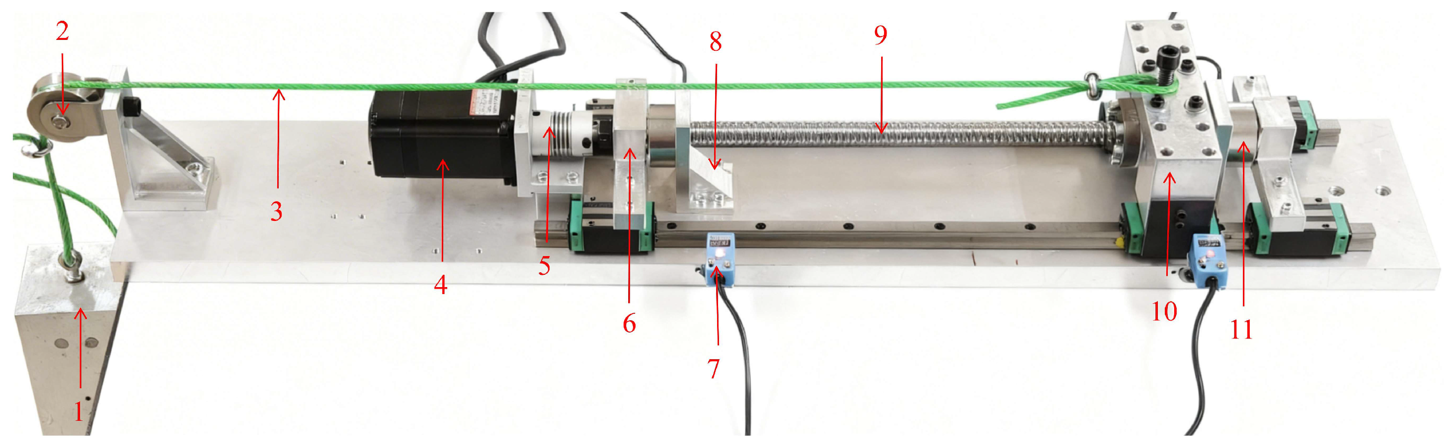
Figure 2.
AE sensor arrangement and shaft pre-tensioning structure.
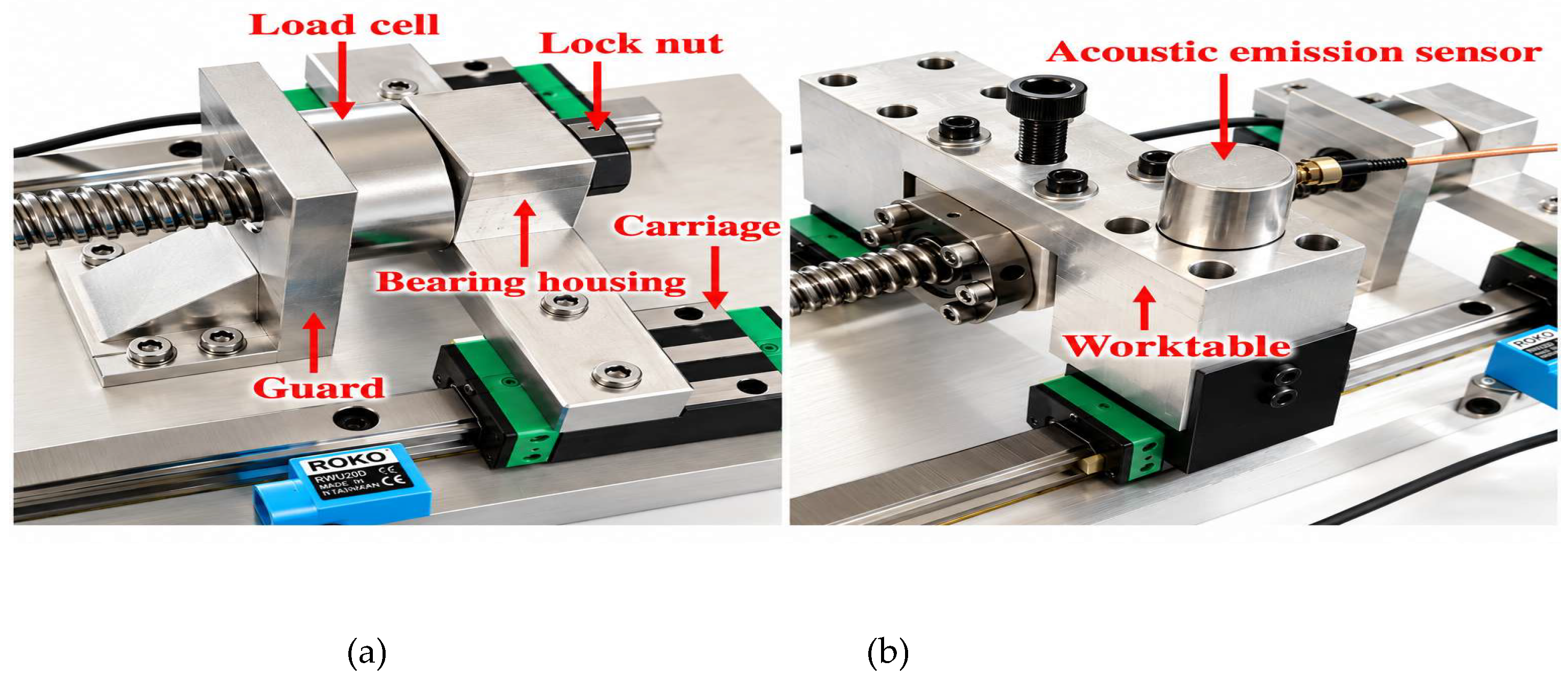
Figure 3.
Surface morphology of the four local wear regions. (a) S1-W1; (b) S1-W2; (c) S2-W3; (d) S2-W4. The scale bars and visible boundaries indicate the projected extent of the wear regions.
Figure 3.
Surface morphology of the four local wear regions. (a) S1-W1; (b) S1-W2; (c) S2-W3; (d) S2-W4. The scale bars and visible boundaries indicate the projected extent of the wear regions.
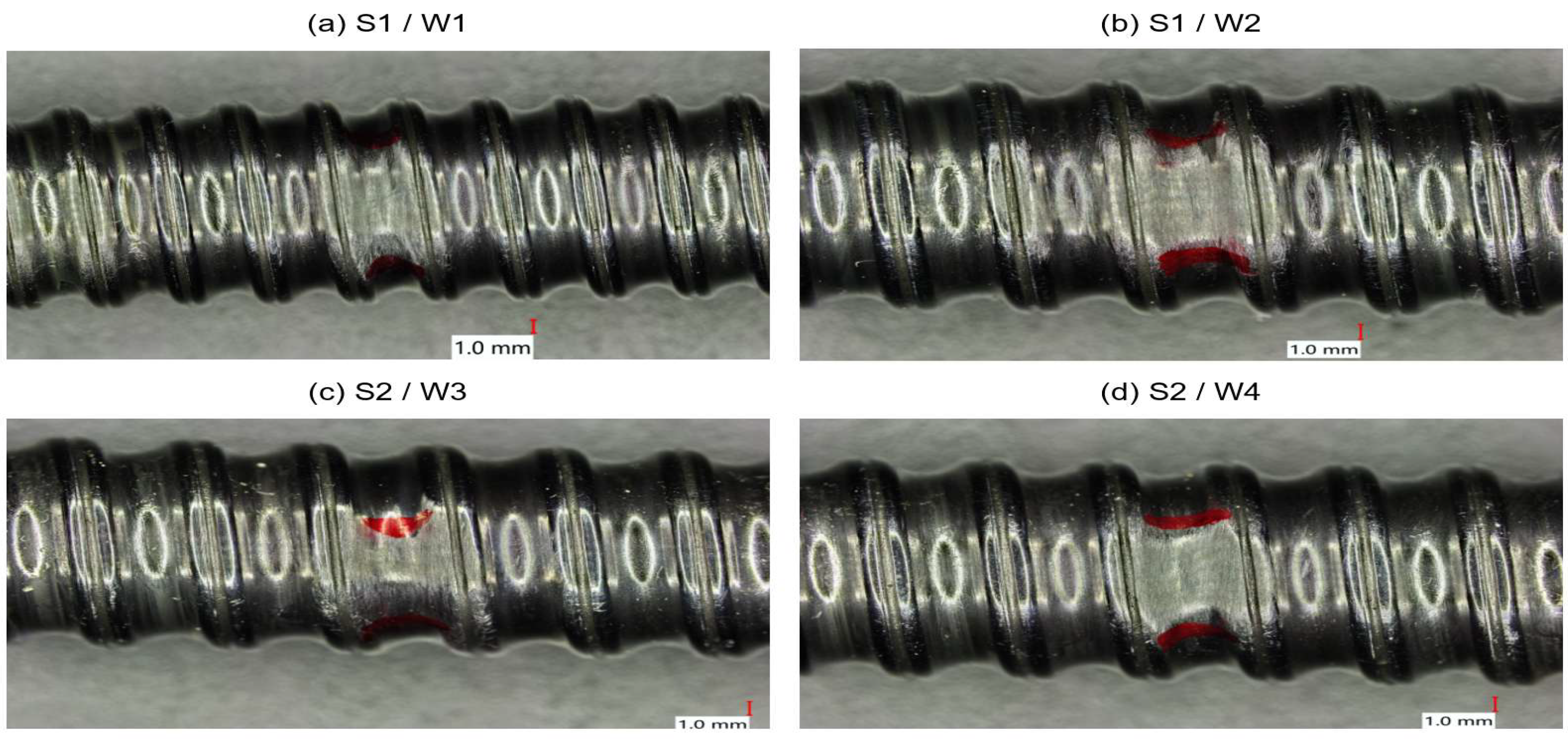
Figure 4.
Raw AE waveforms from healthy and worn states under the same operating condition. The upper and lower rows correspond to S1 and S2, respectively. The three columns show the healthy state and the two wear regions of each specimen. The operating condition was a pre-tension force of 25 kgf, a load of 15 kg, and a speed of 400 r/min. The central 100 ms of each signal is shown on the same voltage scale.
Figure 4.
Raw AE waveforms from healthy and worn states under the same operating condition. The upper and lower rows correspond to S1 and S2, respectively. The three columns show the healthy state and the two wear regions of each specimen. The operating condition was a pre-tension force of 25 kgf, a load of 15 kg, and a speed of 400 r/min. The central 100 ms of each signal is shown on the same voltage scale.
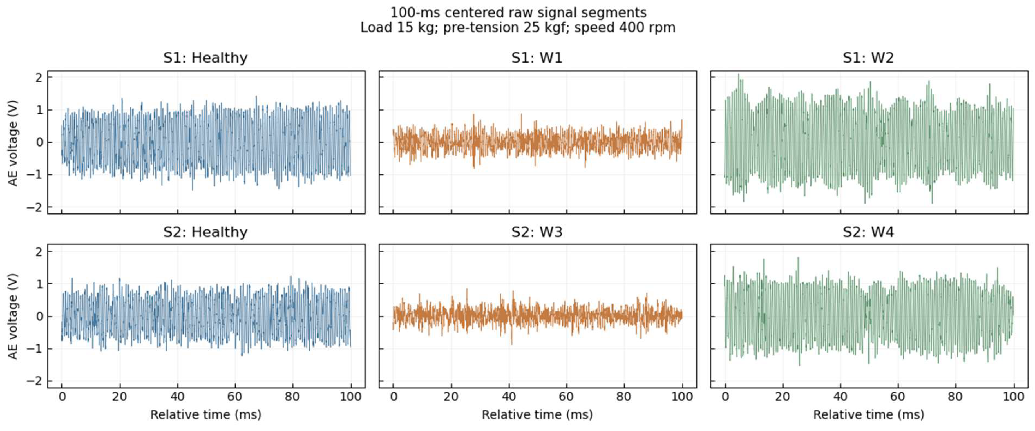
Figure 5.
Healthy AE PSDs of S1 and S2 under different operating conditions.
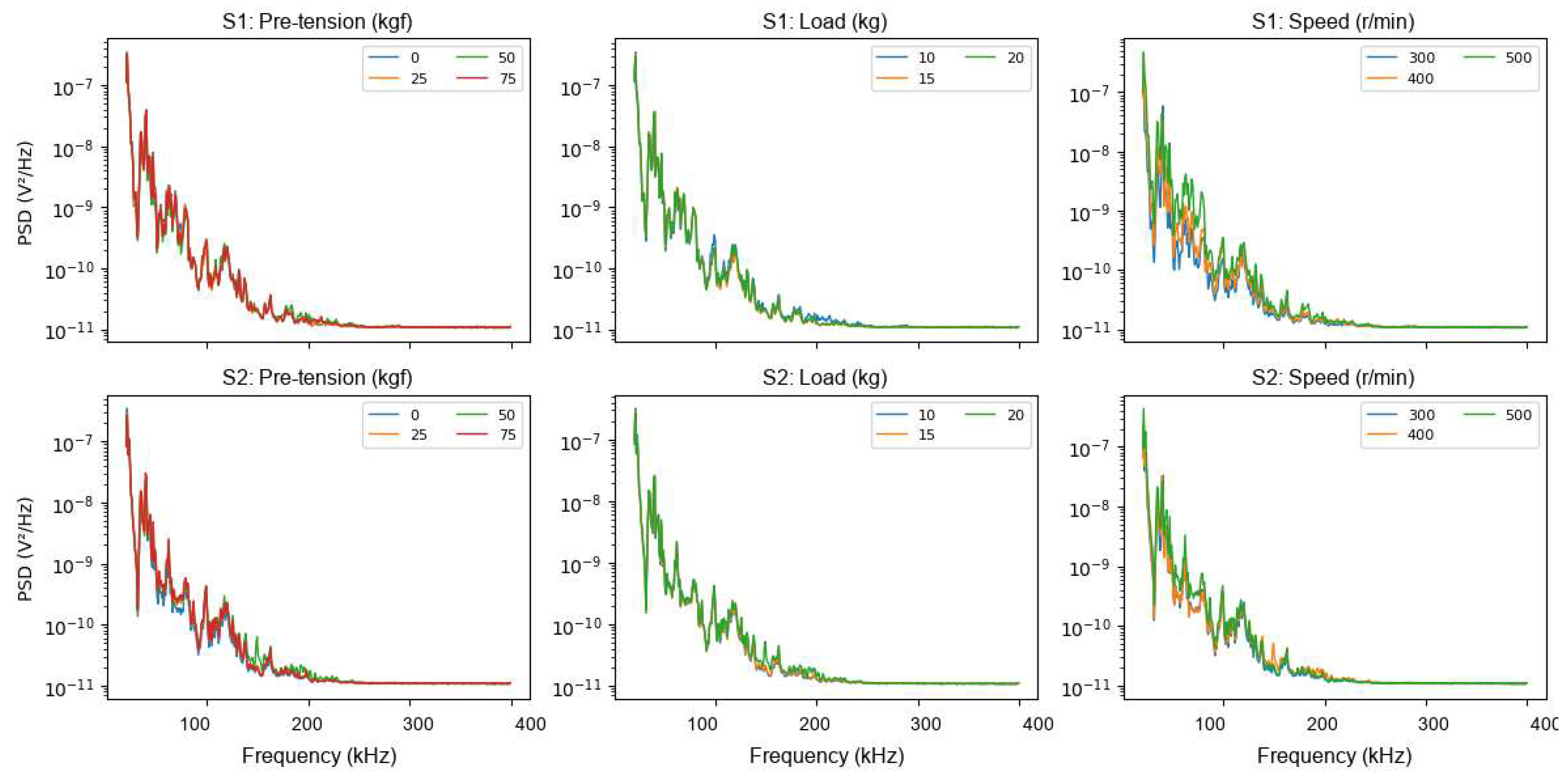
Figure 6.
Healthy AE power in the 20–400 kHz band for S1 and S2 at different speeds.
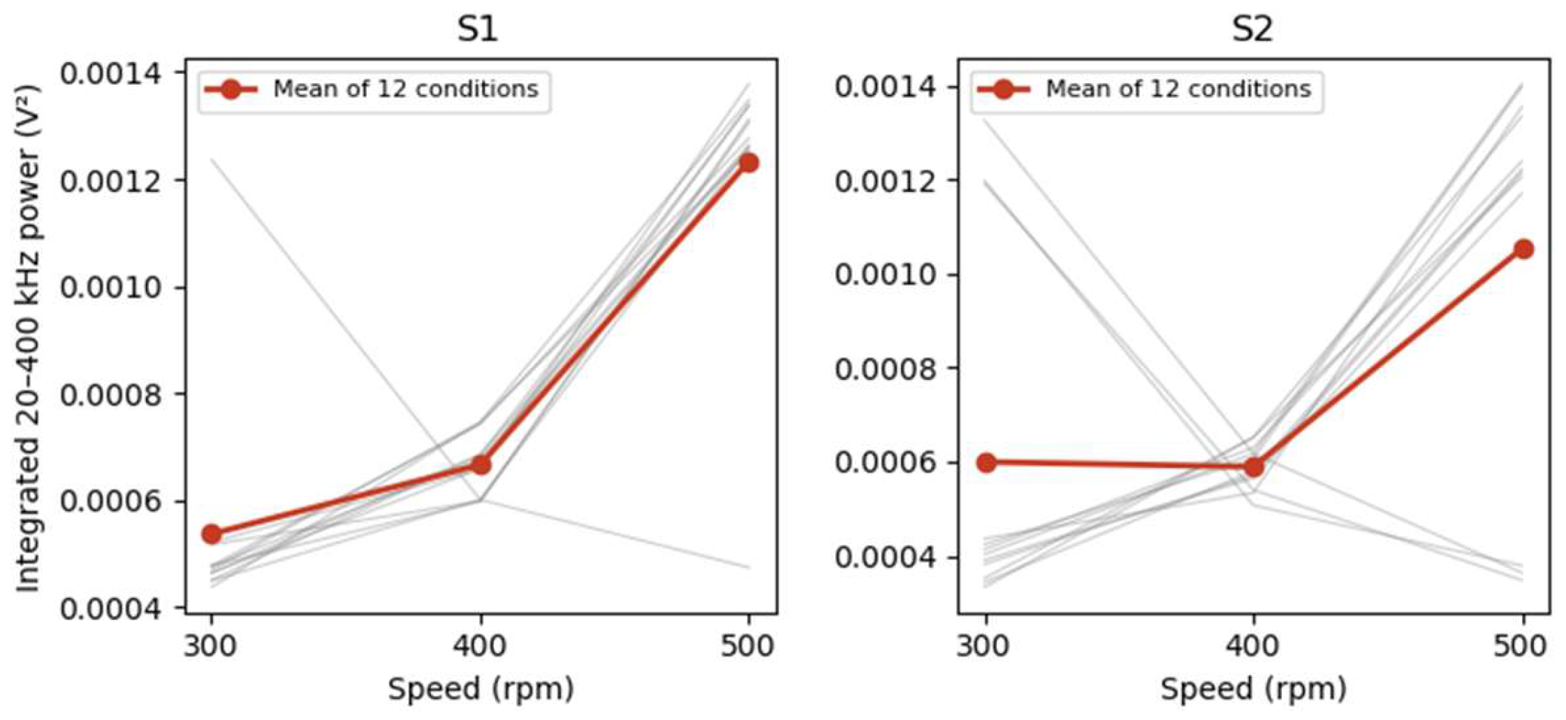
Figure 7.
Mean PSDs and band-power comparisons between the four wear regions and the healthy state. The rows show S1-W1, S1-W2, S2-W3, and S2-W4 from top to bottom. The left column shows healthy and worn PSDs averaged over 36 conditions. The right column shows the 20–400 kHz power log2 ratio for each condition, with rows representing pre-tension force and columns representing load–speed combinations.
Figure 7.
Mean PSDs and band-power comparisons between the four wear regions and the healthy state. The rows show S1-W1, S1-W2, S2-W3, and S2-W4 from top to bottom. The left column shows healthy and worn PSDs averaged over 36 conditions. The right column shows the 20–400 kHz power log2 ratio for each condition, with rows representing pre-tension force and columns representing load–speed combinations.
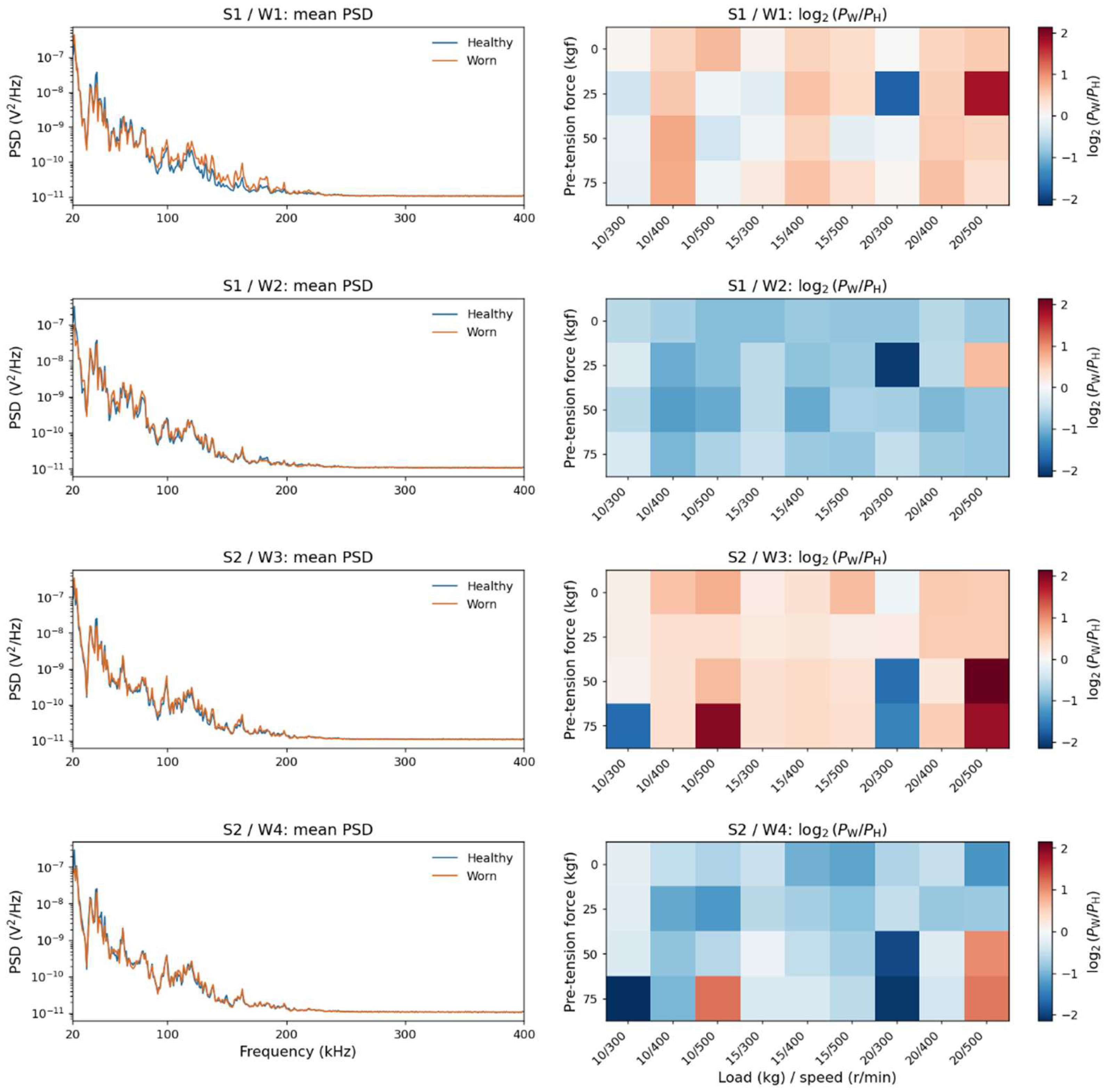
Figure 8.
Relationship between overall and local band-power changes under individual operating conditions.
Figure 8.
Relationship between overall and local band-power changes under individual operating conditions.
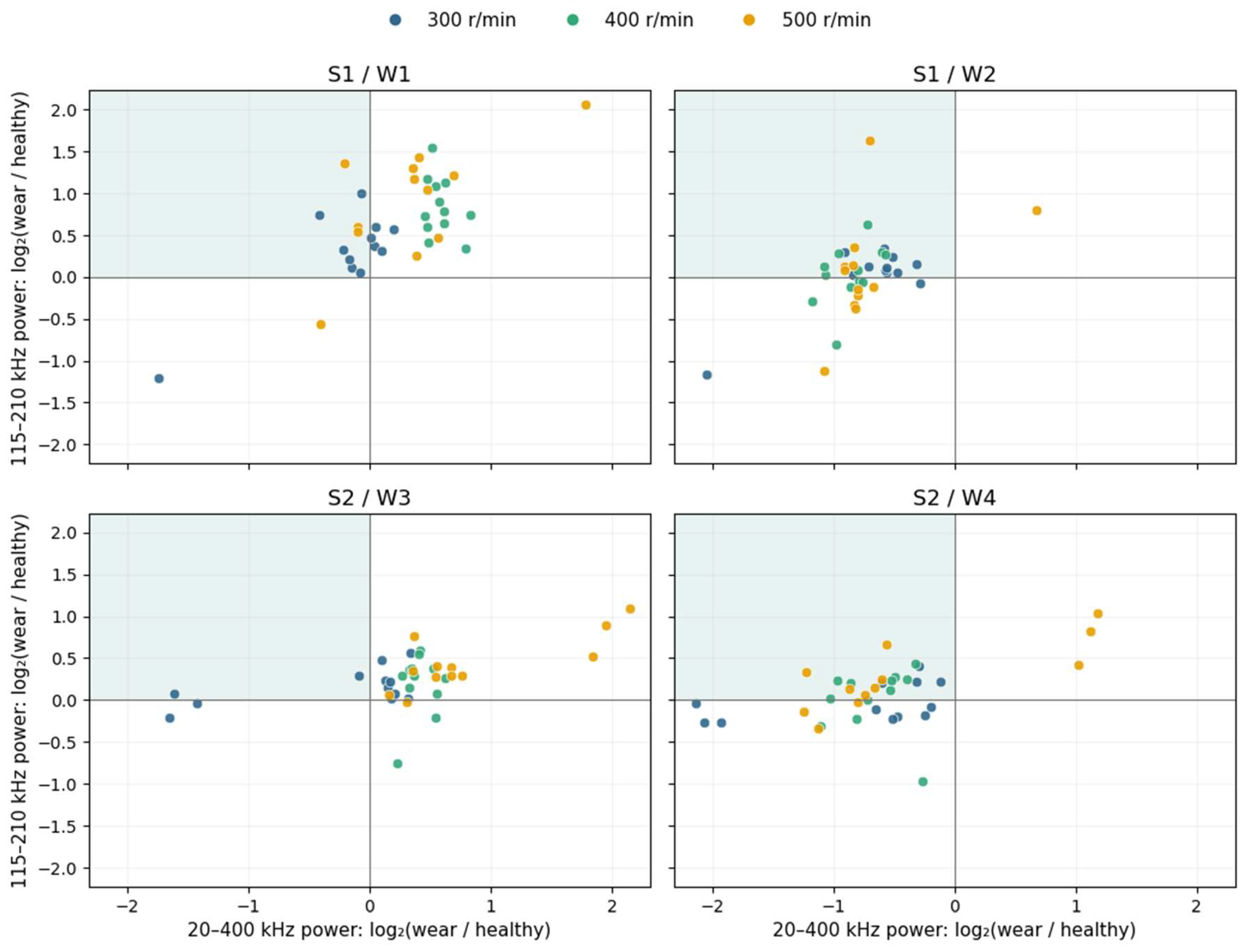
Figure 9.
Effect of healthy signal segment position on power comparisons. The upper and lower rows correspond to 20–400 kHz overall power and 115–210 kHz local band power, respectively. The four columns show S1-W1, S1-W2, S2-W3, and S2-W4. Each point represents one operating condition, and color indicates speed. The vertical coordinate is the median power log2 ratio over different healthy segments for that condition; error bars span the 25th to 75th percentiles.
Figure 9.
Effect of healthy signal segment position on power comparisons. The upper and lower rows correspond to 20–400 kHz overall power and 115–210 kHz local band power, respectively. The four columns show S1-W1, S1-W2, S2-W3, and S2-W4. Each point represents one operating condition, and color indicates speed. The vertical coordinate is the median power log2 ratio over different healthy segments for that condition; error bars span the 25th to 75th percentiles.
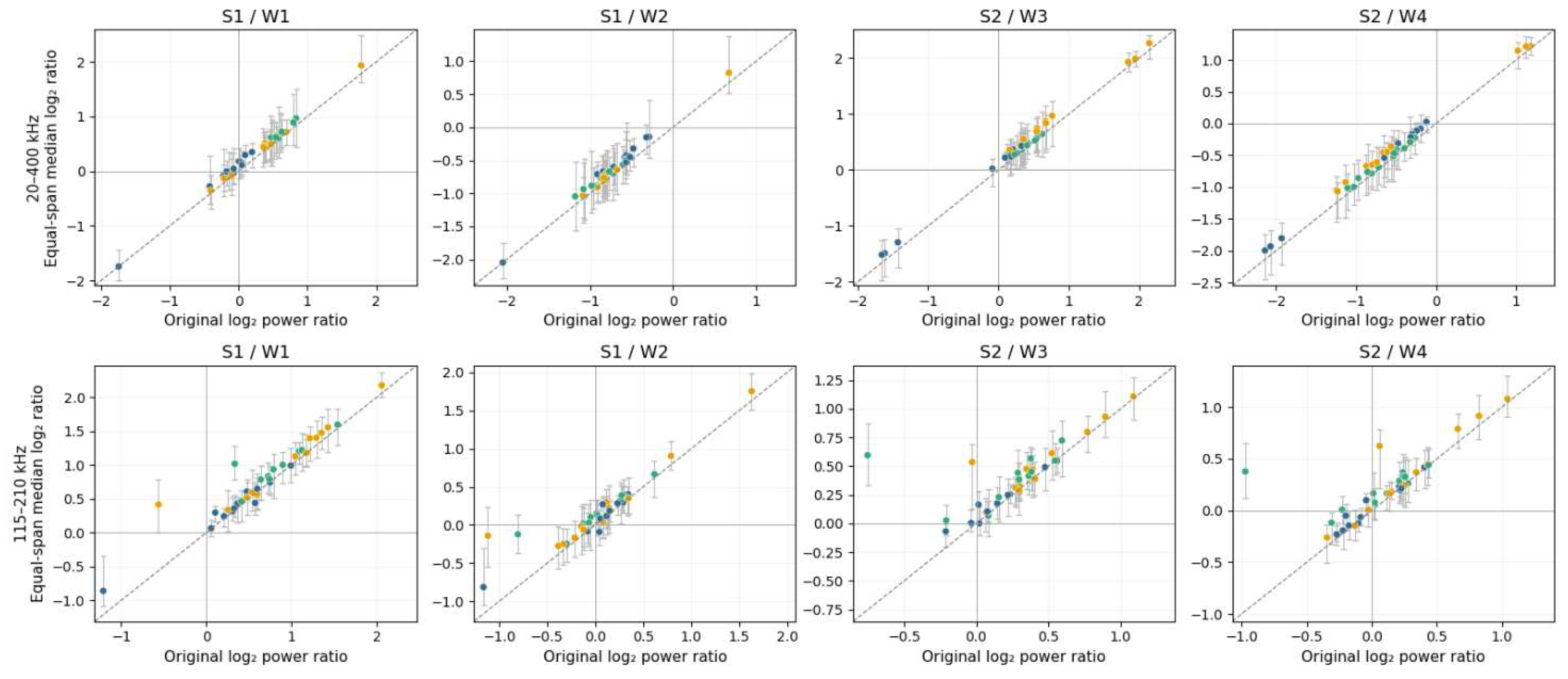
Figure 10.
Input processing and architecture of CP-RNM.
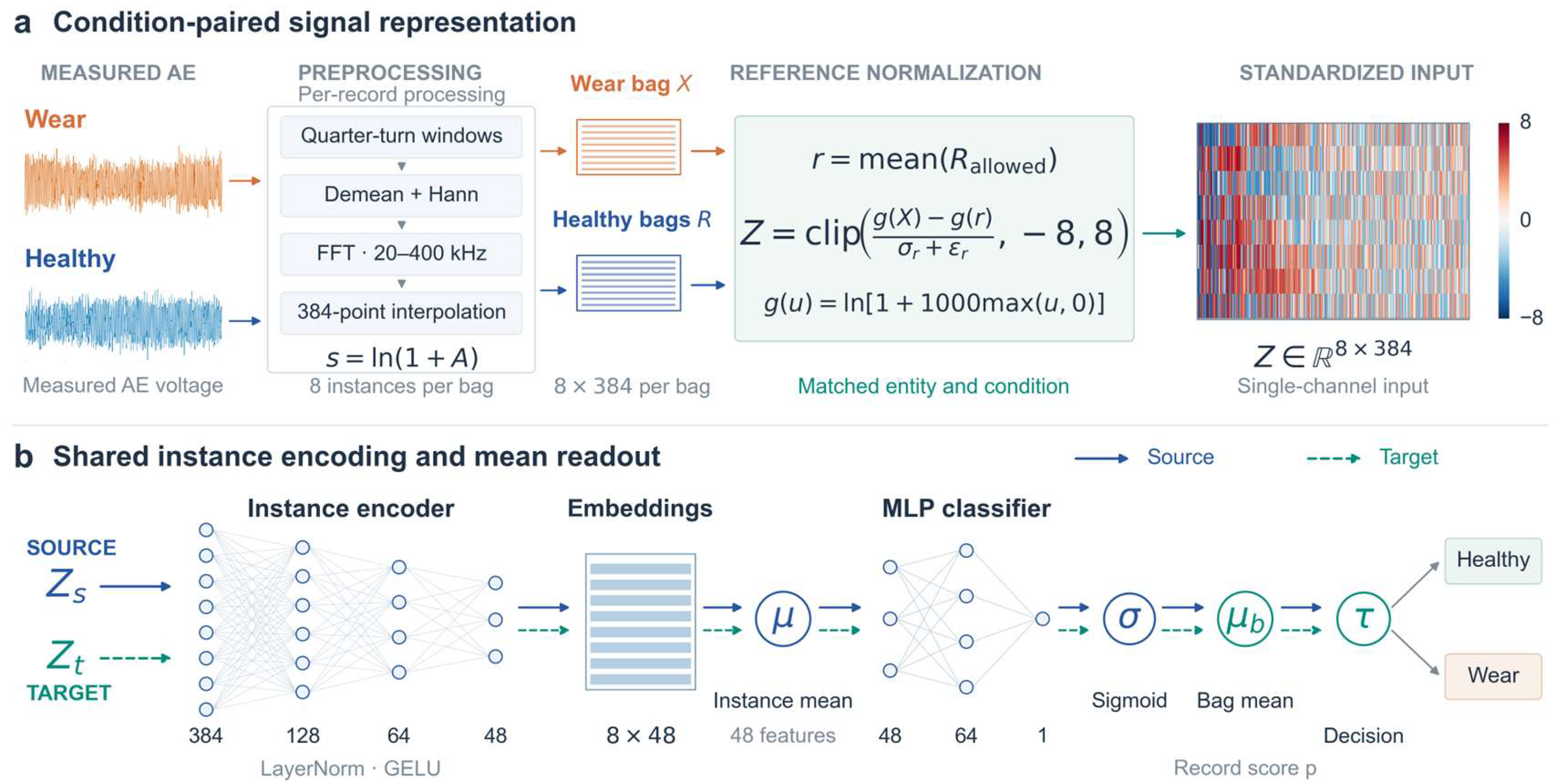
Figure 11.
Operating-condition splits for the three cross-specimen transfer tasks. S1 → S2 is shown as an example; the reverse direction used the same rules. Blue indicates factor levels available for source-domain training and validation, orange indicates target test levels, and gray strikethrough indicates excluded levels. One held-out example is shown for each of Tasks B and C; the complete experiments traversed all held-out levels or target conditions.
Figure 11.
Operating-condition splits for the three cross-specimen transfer tasks. S1 → S2 is shown as an example; the reverse direction used the same rules. Blue indicates factor levels available for source-domain training and validation, orange indicates target test levels, and gray strikethrough indicates excluded levels. One held-out example is shown for each of Tasks B and C; the complete experiments traversed all held-out levels or target conditions.
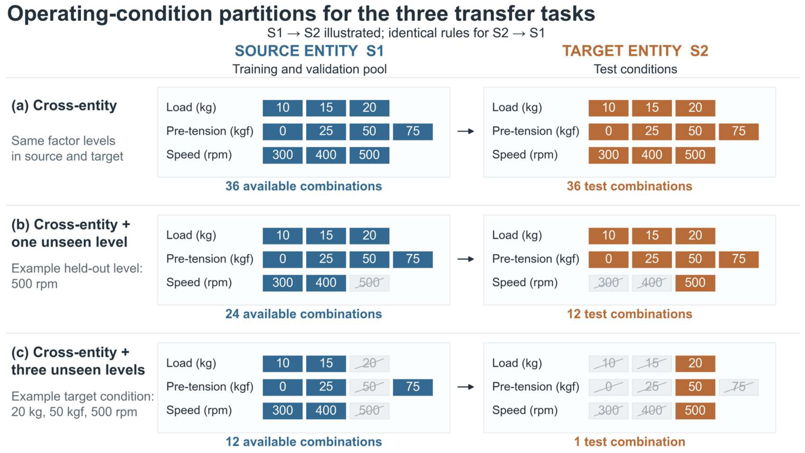
Figure 12.
Bidirectional transfer recognition performance for the three tasks. Note: The four panels show AUC, BACC, wear recall, and healthy specificity. Bar heights are means across five seeds, and error bars are sample standard deviations.
Figure 12.
Bidirectional transfer recognition performance for the three tasks. Note: The four panels show AUC, BACC, wear recall, and healthy specificity. Bar heights are means across five seeds, and error bars are sample standard deviations.
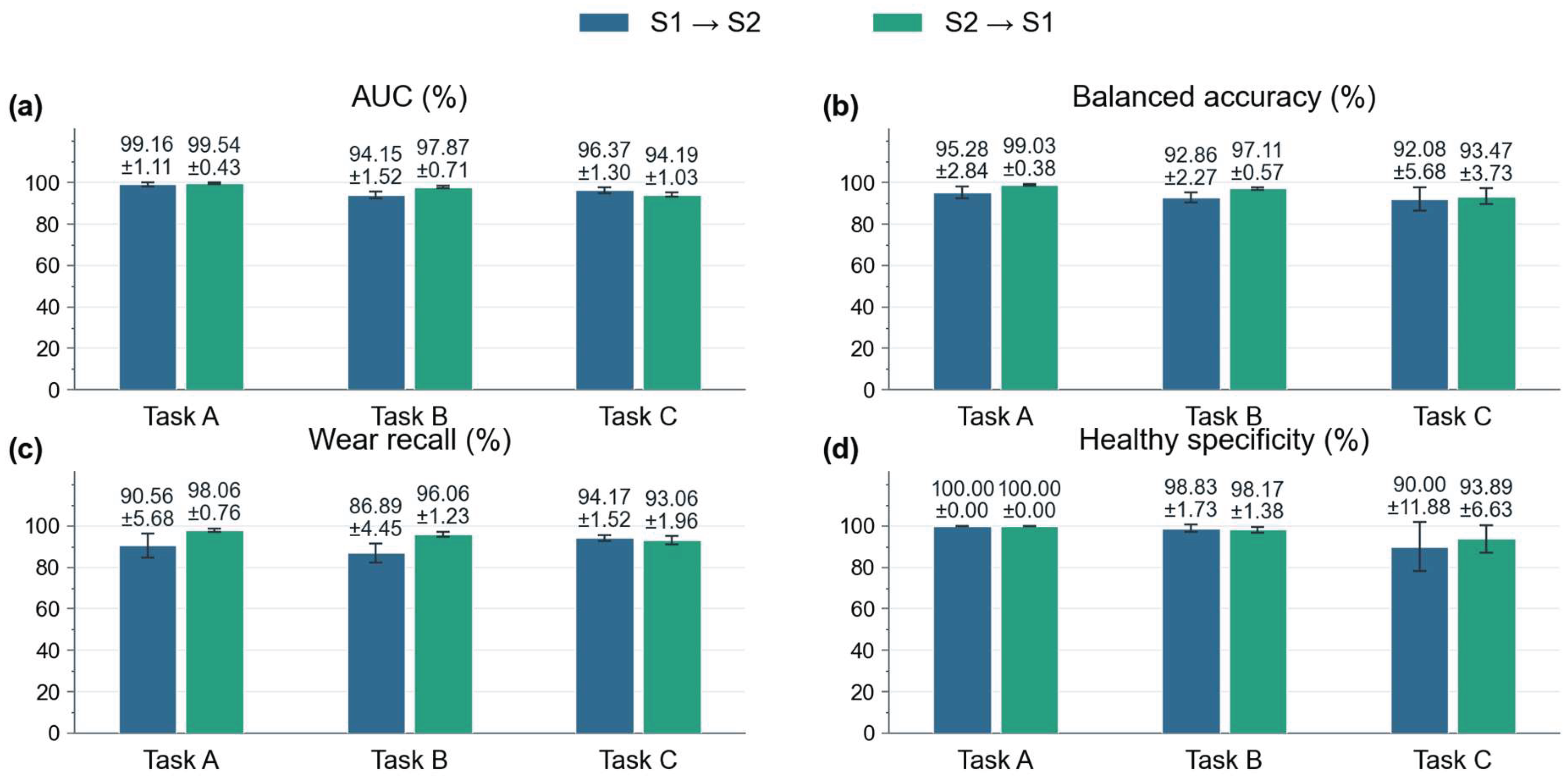
Table 1.
Full factorial operating conditions.
| Operating factor | Levels |
|---|---|
| Shaft pre-tension force (kgf) | 0、25、50、75 |
| Load (kg) | 10、15、20 |
| Speed (r/min) | 300、400、500 |
Note: The three factors were combined in a full factorial design, yielding 36 operating conditions. Both S1 and S2 covered all conditions.
Table 3.
Healthy AE spectral distances associated with operating-condition and specimen differences.
Table 3.
Healthy AE spectral distances associated with operating-condition and specimen differences.
| Comparison factor | Specimen | DASD | DTV |
| Specimen | S1、S2 | 0.31086 ± 0.23958 | 0.18908 ± 0.12446 |
| Pre-tension force | S1 | 0.15863 ± 0.21028 | 0.10761 ± 0.12320 |
| Pre-tension force | S2 | 0.25907 ± 0.29088 | 0.14061 ± 0.14124 |
| Load | S1 | 0.15508 ± 0.21853 | 0.09970 ± 0.12662 |
| Load | S2 | 0.23245 ± 0.27756 | 0.12990 ± 0.13307 |
| Speed | S1 | 0.54513 ± 0.15627 | 0.33317 ± 0.11339 |
| Speed | S2 | 0.53145 ± 0.15331 | 0.27140 ± 0.10695 |
Values are the mean ± sample standard deviation of the paired distances. Both measures are dimensionless.
Table 4.
Band-power and spectral-shape changes in each wear region relative to the healthy state (20–400 kHz).
Table 4.
Band-power and spectral-shape changes in each wear region relative to the healthy state (20–400 kHz).
| Wear region | Wear/healthy power log2 ratio | Median power log2 ratio [Q25, Q75] | Conditions with increased/decreased power | DTV |
| S1-W1 | 0.2425 ± 0.5480 | 0.3738 [−0.0805, 0.5488] | 25/11 | 0.2456 ± 0.1057 |
| S1-W2 | −0.7585 ± 0.3838 | −0.7997 [−0.9076, −0.5813] | 1/35 | 0.2591 ± 0.1168 |
| S2-W3 | 0.3343 ± 0.7596 | 0.3369 [0.1726, 0.5468] | 32/4 | 0.2447 ± 0.1277 |
| S2-W4 | −0.6149 ± 0.7160 | −0.6053 [−0.8976, −0.3238] | 3/33 | 0.2580 ± 0.0803 |
Note: Q25 and Q75 are the 25th and 75th percentiles, respectively, enclosing the middle 50% of the results.
Table 5.
Frequency-band power changes in each wear region relative to the healthy state.
| Wear region | Frequency band (kHz) | Median power log2 ratio [Q25, Q75] | Conditions with increased/decreased power |
|---|---|---|---|
| S1-W1 | 20–115 | 0.3727 [−0.0853, 0.5477] | 25/11 |
| S1-W1 | 115–210 | 0.6169 [0.3572, 1.0943] | 34/2 |
| S1-W1 | 210–305 | 0.0426 [0.0093, 0.0768] | 31/5 |
| S1-W1 | 305–400 | −0.0017 [−0.0116, 0.0046] | 15/21 |
| S1-W2 | 20–115 | −0.8063 [−0.9136, −0.5917] | 1/35 |
| S1-W2 | 115–210 | 0.0790 [−0.1216, 0.2412] | 23/13 |
| S1-W2 | 210–305 | −0.0082 [−0.0248, 0.0010] | 10/26 |
| S1-W2 | 305–400 | −0.0002 [−0.0069, 0.0108] | 17/19 |
| S2-W3 | 20–115 | 0.3372 [0.1742, 0.5483] | 32/4 |
| S2-W3 | 115–210 | 0.2925 [0.0806, 0.3932] | 31/5 |
| S2-W3 | 210–305 | 0.0012 [−0.0070, 0.0156] | 19/17 |
| S2-W3 | 305–400 | −0.0026 [−0.0092, 0.0058] | 14/22 |
| S2-W4 | 20–115 | −0.6133 [−0.9063, −0.3308] | 3/33 |
| S2-W4 | 115–210 | 0.1246 [−0.1423, 0.2534] | 22/14 |
| S2-W4 | 210–305 | 0.0074 [−0.0100, 0.0196] | 22/14 |
| S2-W4 | 305–400 | 0.0006 [−0.0071, 0.0080] | 18/18 |
Table 6.
Numbers of conditions exhibiting simultaneous overall power reduction and local band-power increase.
Table 6.
Numbers of conditions exhibiting simultaneous overall power reduction and local band-power increase.
| Wear region | Overall decrease and local increase | Overall decrease ≥10% and local increase ≥10% |
|---|---|---|
| S1-W1 | 9 | 4 |
| S1-W2 | 22 | 11 |
| S2-W3 | 2 | 0 |
| S2-W4 | 19 | 13 |
Note: Each wear region covered 36 operating conditions. Overall power refers to 20–400 kHz, and local band power refers to 115–210 kHz.
Table 7.
Model and optimization settings.
| Item | Setting |
|---|---|
| Signal windows and input | Quarter revolution; 8 spectra; 384 frequency points; 20–400 kHz |
| Input matrices | Up to 24 bags for >12 signal windows; 1 bag for 8–12 windows |
| Spectral encoder | 384→128→64→48;LayerNorm;GELU |
| Classification head | 48 → 64 → 1; mean of 8 encoded vectors; mean predicted probability within each acquisition |
| Dropout | 0.15 after the first encoder activation and in the classification-head hidden layer |
| Optimizer | AdamW; learning rate 10−3; weight decay 10−4 |
| Batch size and gradient clipping | Batch size = 32; gradient norm limited to 5 |
| Training epochs | Maximum 100 epochs; stop after 15 consecutive epochs without improvement in source validation AUC |
| Model selection | Acquisition-level validation AUC; improvement tolerance 10−5 |
| Classification threshold | 2nd–98th percentiles of validation probabilities at one-percentile-point intervals; remove duplicates; maximize BACC; resolve ties by proximity to 0.5 |
| Reporting seeds | 31、42、73、101、123 |
Table 8.
Bidirectionally averaged performance for the three tasks.
| Task | AUC % | BACC % | Wear recall (%) | Healthy specificity (%) |
|---|---|---|---|---|
| Cross-specimen (Task A) | 99.35 ± 0.49 | 97.15 ± 1.50 | 94.31 ± 3.00 | 100.00 ± 0.00 |
| Cross-specimen + one unseen factor (Task B) | 96.01 ± 0.90 | 94.99 ± 1.14 | 91.47 ± 2.14 | 98.50 ± 0.45 |
| Cross-specimen + three jointly unseen factors (Task C) | 95.28 ± 0.58 | 92.78 ± 1.67 | 93.61 ± 1.24 | 91.94 ± 4.33 |
Note: Values are the mean ± sample standard deviation across five seeds, expressed as percentages.
Table 9.
Bidirectionally averaged Task C results for different reference processing methods.
| Setting | AUC % | BACC % | Wear recall (%) | Healthy specificity (%) |
|---|---|---|---|---|
| Main model | 95.28 ± 0.58 | 92.78 ± 1.67 | 93.61 ± 1.24 | 91.94 ± 4.33 |
| No reference | 62.68 ± 3.89 | 58.33 ± 2.97 | 53.06 ± 5.63 | 63.61 ± 6.76 |
| Mismatched reference | 68.57 ± 2.89 | 61.74 ± 4.01 | 57.08 ± 7.11 | 66.39 ± 13.90 |
| Logarithmic difference | 89.22 ± 3.67 | 79.79 ± 5.17 | 85.14 ± 6.45 | 74.44 ± 8.13 |
Disclaimer/Publisher’s Note: The statements, opinions and data contained in all publications are solely those of the individual author(s) and contributor(s) and not of MDPI and/or the editor(s). MDPI and/or the editor(s) disclaim responsibility for any injury to people or property resulting from any ideas, methods, instructions or products referred to in the content. |
© 2026 by the authors. Licensee MDPI, Basel, Switzerland. This article is an open access article distributed under the terms and conditions of the Creative Commons Attribution (CC BY) license (http://creativecommons.org/licenses/by/4.0/).
Copyright: This open access article is published under a Creative Commons CC BY 4.0 license, which permit the free download, distribution, and reuse, provided that the author and preprint are cited in any reuse.