

Submitted:
13 November 2026
Posted:
16 November 2026
You are already at the latest version
Abstract
Developing automated systems for biomedical image analysis requires datasets that reflect the diversity of the objects under study. When access to clinical data is limited, synthetic structures generated by mathematical models can supplement these datasets. This study presents a modified hybrid angiogenesis model for generating two-dimensional retinal vascular structures. All simulations used the same spatial arrangement of the optic disc, macular region, and foveal avascular zone. The model first generates major vascular trajectories and then grows small branches from the resulting network. In the second stage, local sources are deactivated when they are covered by growing vessel trajectories. Bayesian optimization based on Gaussian process regression was used to select four parameters governing the second stage. The objective function quantifies discrepancies in morphometric and fractal characteristics between simulated vascular masks and reference masks from the publicly available DRIVE dataset. Bayesian optimization and random search started from the same initial sample and used the same number of additional objective function evaluations. Across five new stochastic realizations, the mean loss for the parameter set selected by Bayesian optimization was 12.40% lower than for the baseline parameter set and 8.51% lower than for the set selected by random search. The reduction in overall loss was driven primarily by closer agreement in fractal characteristics, while discrepancies increased for some morphometric characteristics.
Keywords:
retinal vasculature
; hybrid angiogenesis model
; synthetic vascular structures
; Bayesian optimization
; Gaussian process regression
; morphometric analysis
; fractal analysis
1. Introduction
In biomedical practice, many researchers have proposed the use of automated systems for segmenting anatomical structures and quantitatively assessing their characteristics [1]. The development and testing of such systems require datasets that reflect the diversity of the objects under study. Corresponding annotations are also needed when training supervised machine learning models, including neural networks. However, compiling the required datasets may be hindered by limited access to clinical data, the labor-intensive nature of expert assessment, and insufficient available data [2]. Generating synthetic data is one way to expand the available datasets. Such data are generated using mathematical models of the mechanisms underlying biomedical structure formation, generative machine learning models, and approaches that combine simulation with learning from data [3]. Continuum, discrete, or hybrid models are used to describe structure formation mechanisms. Varying their parameters makes it possible to generate structures with different characteristics and investigate the relationship between prescribed conditions and generation outcomes. The applicability of synthetic data depends on how closely their properties match those of real objects and is evaluated in the context of the task considered.
Quantitative characterization of the retinal vascular network is of interest for medical image analysis and the development of mathematical models of branching structures. The geometry of the vascular network is characterized by the distribution of vessels in the image plane, branching patterns, and spatial heterogeneity. Studies of structures of this type have used morphometric methods and fractal analysis to obtain quantitative estimates from visual representations [4,5]. Mathematical modeling, in turn, allows vascular structure formation to be investigated under prescribed conditions and the results to be compared with images of real vascular networks.
The studies reported in [6,7,8] provide an example of using mathematical modeling to investigate structural characteristics. In this series of studies, the authors proposed a discrete–continuum angiogenesis model. In [6], a model of tumor angiogenesis was proposed that accounts for random endothelial cell motility, chemotaxis, and haptotaxis. The discrete formulation made it possible to track the movement of individual vessel tips and the formation of the capillary network. The authors subsequently extended the model to include blood flow calculations in the generated networks [7]. Later, drug delivery through two- and three-dimensional vascular networks was investigated in [8]. Numerical experiments showed that selective removal of vessels with low blood flow can accelerate drug delivery, whereas removing vessels with high blood flow can cause perfusion of the modeled capillary bed to cease.
A hybrid approach to retinal vascular network development was considered in [9]. The authors proposed a two-dimensional model of superficial vascular plexus formation in the mouse retina, combining a continuum description of biochemical fields with a discrete representation of astrocyte and endothelial tip movement. Blood flow, vascular adaptation, and structural remodeling were taken into account during network development. The resulting vascular configurations were compared with experimental retinal specimens at different developmental stages. The authors demonstrated agreement between the morphology of the modeled and observed structures, enabling the model to be used to investigate the mechanisms of vascular plexus formation.
A model of human retinal vascular network formation that accounts for endothelial cell movement and astrocyte dynamics was proposed in [10]. Astrocytes were treated as a structure that guides vascular growth and restricts vessel penetration into the foveal region. Within this framework, the authors reproduced the superior and inferior temporal arcades, the foveal avascular zone, and the radial orientation of vessels toward its boundary. The simulation results made it possible to investigate the role of the spatiotemporal dynamics of astrocytes in the formation of the characteristic vascular pattern.
Retinal hemodynamics were modeled in [11]. Blood flow is described using an electrical circuit analogy, in which changes in vascular resistance are linked to intraocular pressure and autoregulation of vessel diameter. The calculations showed that the response of retinal blood flow to changes in intraocular pressure depends on arterial pressure and the state of autoregulation. In [12], blood flow modeling was coupled with oxygen transport in multilayered retinal tissue. Arterial and venous vessels are represented as fractal trees, whereas capillary vessels are described using a lumped-parameter model. The analysis allowed the effects of arterial pressure, plasma viscosity, tissue oxygen consumption, and arteriolar wall permeability to oxygen on oxygenation measures to be assessed.
Studies have also explored the generation of synthetic structures to expand the datasets available for analysis. In [3], the authors proposed a model of the retinal vascular network comprising arterial and venous trees connected by capillary vessels. The trees were constructed using constrained constructive optimization, and the network geometry accounted for the location of the optic disc and the macular region. The resulting structures were used to generate additional data and develop algorithms for their analysis.
Various quantitative measures are used to analyze clinical images and compare modeled structures. Morphometric measures are used, for example, to compare clinical images with modeled structures. These include the fraction of image area occupied by vessels, the total length of the vascular network, branch point density, and vessel tortuosity.
Fractal analysis complements these morphometric measures. A foundational review of fractal analysis of the retinal vascular system was presented in [4], showing that fractal dimension can serve as a quantitative measure of vascular architecture. In our previous studies [13], fractal analysis and neural networks were used to classify computed tomography images of the lungs. A hybrid machine learning system based on multifractal features was subsequently developed for glaucoma diagnosis from retinal images [14]. Fractal dimension characterizes the scaling properties of the vascular network, but its value alone is insufficient to fully describe spatial heterogeneity. Structures that differ in vessel arrangement and branching patterns can have similar values of this measure. Multifractal analysis provides a more detailed description by considering a spectrum of generalized dimensions [5,15]. This approach has been applied to the analysis of retinal images [5,16] and computed tomography images of the lungs [17].
Generating synthetic vascular structures with prescribed characteristics requires the selection of appropriate model parameters. In a stochastic formulation, a single parameter set can produce different network realizations, which must be taken into account when comparing the results with reference vessel masks. Therefore, alongside model development, the problem of parameter selection based on the quantitative characteristics of the generated structures is considered.
The aim of this study is to further develop a hybrid model for the formation of two-dimensional retinal vascular structures and to devise a procedure for selecting its control parameters using machine learning methods. Model calibration is based on comparing the morphometric and fractal characteristics of the generated structures with those of reference vessel masks. The main focus is on the effects of the parameters on network geometry and the variability of its quantitative characteristics across stochastic realizations.
2. Mathematical Formulation of the Continuum Model of Retinal Angiogenesis
The baseline model used in this study is the continuum–discrete angiogenesis model of Anderson and Chaplain [6]. Its continuum formulation is recalled below, followed by the modifications introduced for retinal vasculature. The hybrid model describes the spatiotemporal dynamics of endothelial cell density , the concentration of tumor angiogenic factors (TAF) , and the fibronectin concentration . Cell migration is described in terms of random motility, chemotaxis along the angiogenic factor gradient, and haptotaxis along the fibronectin gradient. The rules governing the movement of cells at sprout tips are derived from a finite-difference approximation of the continuum model. Additional rules for branching, anastomosis, and cell proliferation are specified in the discrete model.
To obtain a dimensionless formulation, the spatial coordinates are scaled by the distance L between the parent vessel and the tumor, and time is scaled by the characteristic time scale . Endothelial cell density and the concentrations are scaled by the corresponding characteristic values , , and . Dimensionless variables are used hereafter.
is the dimensional TAF diffusion coefficient. Asterisks denote characteristic values to distinguish them from the initial distribution functions.
The relationships between the coefficients are given below:
Here, is the coefficient of random endothelial cell motility, is the maximum dimensional chemotactic sensitivity, and is the dimensional haptotactic sensitivity. The coefficient governs fibronectin production, while and govern endothelial uptake of fibronectin and TAF, respectively. The concentration is the TAF concentration at which the chemotactic sensitivity falls to half its maximum value. The chemotactic sensitivity is defined as , where specifies its maximum value and describes the decrease in sensitivity as the factor concentration increases.
The dimensionless continuum equations of the original model are
The first equation in this system describes changes in endothelial cell density:
Here:
- , the first term, describes the random motility of endothelial cells with control parameter D;
- is the chemotactic term, which specifies directed cell movement along the angiogenic factor concentration gradient;
- is the haptotactic term; for , the haptotactic flux is directed toward increasing fibronectin concentration f.
The continuum system describes the dynamics of endothelial cell density and the associated concentration fields. To reproduce the capillary network, a discrete model based on a finite-difference approximation of the continuum system is used. The model tracks the movement of individual capillary sprouts, and their trajectories determine the geometry of the developing network. Proliferation and anastomosis are also incorporated through discrete rules.
The second equation in system (1) describes fibronectin dynamics:
Fibronectin dynamics are described in terms of its production by endothelial cells, , and its uptake by these cells during migration, .
Before endothelial cell migration begins, the initial TAF distribution is motivated by diffusion and natural decay. In dimensional variables,
where and are the dimensional TAF concentration and time, acts on the dimensional spatial coordinates, and is the natural decay coefficient. The initial TAF profile is specified below.
Once migration begins, the model accounts only for endothelial uptake of TAF. In dimensionless variables, this gives
where is the dimensionless uptake coefficient. This equation is included in the dimensionless system (1).
3. Discretization of the Continuum System
3.1. Original Discrete Model
To reproduce the structure of the capillary network, a discrete model based on a finite-difference approximation of the continuum system (1) is used. The model tracks the movement of endothelial cells at capillary sprout tips, and their trajectories determine the geometry of the developing network. As noted above, branching, anastomosis, and proliferation are incorporated through additional rules in the discrete formulation.
The continuum system (1) is discretized using an explicit Euler scheme in time and central-difference approximations of the spatial derivatives. The computations are performed on a uniform grid with spatial and temporal step sizes h and k, respectively. After discretization, the equation for endothelial cell density takes the form:
The quantity denotes the grid value of endothelial cell density. In this notation, the indices correspond to the planar coordinates , respectively. The coefficients depend on the TAF and fibronectin concentrations at the current and neighboring grid nodes at time step q, as well as on the model parameters and the spatial and temporal step sizes. In the discrete model, these coefficients are used to assign relative weights to possible cell movements.
The coefficients are obtained by substituting central-difference approximations of the spatial derivatives into the continuum equation and collecting terms of second order in h. Each of the coefficients includes contributions from random motility, chemotaxis, and haptotaxis:
where is the chemotactic sensitivity function; D is the diffusion coefficient; is the haptotaxis coefficient; and k and h are the temporal and spatial step sizes, respectively.
The weights and correspond to leftward movement, , and rightward movement, , respectively. The weights and correspond to upward movement, , and downward movement, , respectively.
The coefficient specifies the relative weight of remaining at the current position. It also includes contributions from random motility, chemotaxis, and haptotaxis:
At each time step, the coefficients are calculated at the current node and used as relative weights of the possible actions. Provided that the coefficients are nonnegative and their sum is positive, the action probabilities are obtained by normalization:
The cumulative sums and the corresponding intervals are defined as:
For a random number U uniformly distributed on , the selected action j satisfies . The values correspond to remaining at the current position and moving left, right, up, and down, respectively. The parameters and discretization step sizes must ensure the admissibility of the weights.
If the angiogenic factor and fibronectin gradients are absent, the coefficients are equal, and tip movement follows a random walk. An angiogenic factor gradient biases the probabilities toward higher TAF concentrations (chemotaxis), whereas a fibronectin gradient biases them toward higher fibronectin concentrations (haptotaxis). When both gradients are present, the bias is determined by their combined effect.
The full discrete system also includes the equations for fibronectin and TAF:
A discrete counterpart of the no-flux boundary condition for endothelial cells is imposed at the boundary of the computational domain. The transition rules confine cell movement to the simulation domain.
3.2. Branching and Anastomosis Rules
Branching occurs at the tip of an existing sprout. In the original study, three conditions were specified that must be satisfied for sprout branching:
- 1.
- the sprout age must exceed the prescribed threshold ; a newly formed sprout must reach the prescribed age before it can branch;
- 2.
- sufficient free space must be available around the sprout tip; branching into an area occupied by another sprout is not allowed;
- 3.
- the endothelial cell density must exceed the threshold , where .
When all three branching conditions are satisfied, each sprout tip generates a new branch with probability . This probability is considered an increasing function of the TAF concentration: higher TAF concentrations correspond to a higher branching probability.
3.3. Anastomosis and Proliferation Rules
Vascular anastomosis is modeled as the joining of two capillary vessels upon contact. The model assumes that, after two tips merge, only one of the two sprouts, selected at random, continues to grow.
Endothelial cell proliferation is considered separately from migration. In the experimental system considered by the authors, cell division is observed approximately 36–48 hours after the onset of angiogenesis and is localized behind the sprout tip. In the original simulations of Anderson and Chaplain, proliferation is introduced after 48 hours, corresponding to the dimensionless time .
3.4. Discrete Simulation Algorithm
At each time step of the original simulation, the finite-difference scheme coefficients are calculated from the values of the fields and f, and the field values at the next time step are determined. For each active tip, the coefficients corresponding to its position are used to determine the movement direction. A random number is then used to select the movement direction or the action of remaining at the current position. Additional rules are applied for branching, anastomosis, and proliferation.
The discrete model described above provides the mathematical basis for the subsequent modification. The implementation considered here retains the discrete representation of vessel tips and accounts for random motility, chemotaxis, and haptotaxis. The revised movement, branching, and anastomosis rules are described below. The continuum equation for endothelial cell density is not used separately; network growth is determined by the stored tip trajectories. No separate rule for endothelial cell proliferation is used in this implementation.
4. A Two-Stage Model for Retinal Vascular Growth
We extend the Anderson–Chaplain model by introducing a two-stage procedure for generating two-dimensional retinal vascular networks. The geometry of the computational domain is modified by specifying initial vessel tip positions near the optic disc and introducing an exclusion region corresponding to the foveal avascular zone. The initial distributions of the angiogenic signal and fibronectin are also modified, and their reaction terms are coupled to the generated vascular trajectories. The first stage includes signal diffusion and an additional repulsive field near the optic disc. The diameters of new segments are stored when branching occurs. Once the major vascular network has formed, its geometry is fixed, and a second stage of small branch growth driven by local sources is initiated. A binary image of the network is constructed from the stored trajectories and diameters.
4.1. Geometry of the Computational Domain
As described above, the hybrid angiogenesis model is adapted to generate retinal vascular structures. The vascular network is represented by a set of sprout tip trajectories. Initial tip positions and an exclusion region corresponding to the foveal avascular zone are specified to reflect the geometry of the retina.
The unit square
is used as the computational domain, with a uniform grid of nodes. The node coordinates are defined as follows:
where and . All spatial parameters are expressed in dimensionless coordinates.
The initial tips are positioned near the right boundary of the computational domain, close to a point representing the optic disc. In the selected configuration, this point has the coordinates
The seven initial points lie on the vertical segment . Their subsequent movement determines the formation of vascular trajectories within the computational domain.
To account for the foveal avascular zone (FAZ), a circular region is introduced with the following center coordinates and radius:
Here, are the center coordinates, and is the radius.
Thus, the foveal avascular zone is defined as
These dimensions are parameters of the model geometry.
Vessel tips cannot be placed at nodes belonging to , and new branches cannot be formed there. If a transition into this region is selected, the tip remains at its previous position. This restriction applies to the discrete tips, whereas the chemical signal and fibronectin fields are defined throughout .
Once a tip reaches the outer boundary of the computational domain, its movement stops. Its trajectory is retained and included in the final image of the vascular network. A schematic of the computational domain, showing the initial tip positions and the FAZ boundary, is presented in Figure 1.
4.2. Initial Distributions of the Angiogenic Factor and Fibronectin
The initial distributions of the chemical signal and fibronectin specify the spatial conditions for vascular network formation. In the proposed model, c represents the concentration of a generalized angiogenic signal. The initial profiles are defined throughout the computational domain .
The chemical signal distribution is constructed using two profiles. The first profile is defined as
The additional profile has elliptical level curves and is defined as
The profile of the macular region has the same center as the foveal avascular zone and is given by
The resulting initial distribution of the chemical signal is defined by the pointwise maximum:
The pointwise maximum combines the two spatial signal profiles. The common factor reduces their values near the center of the foveal avascular zone. This suppression is imposed in the initial distribution; during subsequent field updates, the concentration in this region may change due to diffusion.
The initial fibronectin distribution is specified by a radial profile centered at , which corresponds to the optic disc region. Let the distance to this point be
The initial fibronectin concentration is defined as
The initial concentration reaches its maximum value of 0.5 at the center of the profile. It decreases linearly with distance from the center to the background value of 0.3, which is reached at . At greater distances, the initial field remains at this value. The background is specified during initialization, whereas subsequent dynamics are governed by the reaction equation.
These distributions define the spatial conditions of the computational experiment. Their shapes and parameters are treated as elements of the model configuration. The initial distributions of the angiogenic signal and fibronectin are shown in Figure 2.
4.3. Field Dynamics and Coupling to the Generated Trajectories
The fields are coupled to the vascular network through a binary indicator of visited nodes. For a node with coordinates , we define
where q is the time step index corresponding to . After a tip moves or stops, the indicator remains equal to one at the nodes it has previously visited. Revisiting a node does not increase this value. Active tip positions are tracked separately when checking contacts and branching conditions.
In the proposed approach, angiogenic signal diffusion is included throughout the first simulation stage. The diffusion rate of the angiogenic factor is specified by an additional dimensionless coefficient , which is treated as a parameter of the computational experiment. The value of is specified empirically and is not derived from physiological measurements of the diffusion coefficient.
The fields are updated using an explicit Euler scheme in time. At interior nodes of the computational domain, the first-stage scheme takes the form
where the discrete Laplacian is defined as
The following coefficient values are used in the computational experiments:
During the first simulation stage, the angiogenic signal concentration at the outer boundary is maintained at its initial value:
The following conditions are checked for the explicit update:
After each update, negative concentration values are set to zero. At each time step, the concentration fields are updated first, with the indicator held fixed. The updated values are then used to process the tips. During a sequential pass through the tips, the chemical fields remain unchanged, while the maps of active tips and trajectories are updated after the corresponding events.
During the second stage, diffusion updates of the field c cease. Small sprout movement is governed by a separate field defined by local sources. The fibronectin field continues to be updated using the same reaction scheme, with all generated trajectories taken into account.
4.4. Tip Movement Probabilities
Five possible actions are considered for each active tip: remaining at its current position or moving to one of the four neighboring nodes. The probabilities are determined by the updated field values at the current node and its neighbors.
A stationary auxiliary field is introduced during the first stage:
The field I introduces an additional bias that directs tips away from the region of growth initiation. It is included as a directional term and is not intended to represent a specific biochemical inhibitor or signaling pathway. The coefficient increases the weights of transitions toward lower values of I. Its value was chosen empirically for the baseline numerical configuration and was not calibrated against physiological measurements. Growth within the foveal avascular zone is restricted separately by a geometric mask. The distribution of the auxiliary field I and the directions of the vector are shown in Figure 3.
To combine the directional effects, we introduce the auxiliary quantities
Here, is the dimensionless chemotactic sensitivity constant. The function satisfies
Thus, differences in account for the concentration dependence of chemotactic sensitivity. No separate equation is solved for ; its values are calculated from the known fields.
For a tip at node , four differences are defined:
For example, for a movement to the right,
The quantity determines the random transition rate in the absence of directional effects. A positive difference increases this rate, whereas a negative difference reduces it. For , we obtain .
The action probabilities over a time step k are
The probability of remaining at the current position is nonnegative provided that
In the implementation, this condition is checked whenever the probabilities are calculated. Random perturbations are not added to the weights, and the probabilities are not subsequently renormalized.
The actions are ordered as remaining in place, moving down, moving up, moving right, and moving left. Denoting the corresponding probabilities by , we define the cumulative sums
A random number is generated, and the action satisfying is selected. Thus, the movement remains stochastic.
The following values are used in the simulations:
If the selected neighboring node belongs to the foveal avascular zone, the transition is rejected, the tip remains at its previous position, and the branching check is skipped for that step. The probabilities are not renormalized over the allowed directions. After an allowed movement, contacts are checked and, if no contact occurs, the tip is checked for arrival at the outer boundary. Upon reaching the boundary, the tip becomes inactive, and its trajectory is retained.
4.5. Branching and Anastomosis Rules
Branching is represented by the formation of a new active tip near an existing tip. Whether branching is permitted depends on tip age, the local angiogenic factor concentration, and the positions of other active tips.
The age of each tip is tracked and set to zero when the tip is created. At each time step, the age of the active tip being processed is increased by k, regardless of whether it moves. Branching is permitted when
An additional requirement is that no other active tips are present in a square neighborhood of nodes centered on the node under consideration. This neighborhood is defined relative to the current tip position after the selected action has been processed, and only nodes within the computational domain are considered. The local angiogenic factor concentration in the updated field must satisfy
If these conditions are met and an available neighboring node exists, a new tip is formed with probability
Here, is the probability of a successful branching trial over the reference time step . For , we obtain . This probability is applied after the age and local conditions have been satisfied; it does not represent the probability of branching at the start of the simulation.
The eight neighboring nodes, including diagonal neighbors, are considered for placement of the new tip. An eligible node lies strictly inside the computational domain, outside the foveal avascular zone, is not occupied by an active tip, and does not belong to a previously generated vascular trajectory. One of the eligible nodes is selected with equal probability. If no such node exists, no branch is created. The age of the new tip is zero, whereas the age of the parent tip is not reset. This branching rule is applied only during the first simulation stage. Occupancy checks use the tip and trajectory maps, including changes made by tips processed earlier in the current time step.
Anastomosis occurs when two active tips come into contact. If the node selected for movement is occupied by another active tip, either tip is selected with equal probability to continue growing. The other tip becomes inactive. The contact node is retained in the network geometry and is represented by one active tip in the occupancy map. After the contact has been processed, the branching check for the moving tip is skipped for the current time step.
Contact between a tip and a previously formed vessel is also considered. If the selected node belongs to a vascular trajectory, is not part of the current sprout’s own history, and is not occupied by another active tip, the arriving tip becomes inactive. Its stored trajectory joins the existing vascular segment. A tip returning to a node on its own trajectory does not stop for this reason alone. Contacts are identified by coincident trajectory nodes; after anastomosis has been processed, the branching check for the moving tip is skipped. Contact between thickened vessel regions in the image is not treated as a separate anastomosis event.
4.6. Assignment of Diameters and Construction of the Binary Mask
A sprout trajectory is represented by a sequence of grid nodes. Two consecutive distinct positions define a line segment, which is assigned the current sprout diameter when it is added. The initial diameter of the original sprouts is grid spacings.
During first-stage branching, diameters are assigned using a geometric rule in the form of a generalized Murray’s law [19]:
which gives
Here, is the diameter before branching, is the diameter of the continuing parent sprout, and is the diameter of the side branch. The values and are used. The diameters of previously stored segments are not modified when a new branch forms. During the first stage, the assigned diameter does not affect tip movement or chemical field updates. During the second stage, the local diameter of the major vessel is taken into account when selecting the initiation site and size of a small sprout. Blood flow and flow-dependent diameter adaptation are not computed in this formulation.
After growth is complete, a binary network mask is constructed. For a segment with endpoints and diameter , we define the region
The vascular mask includes pixels whose centers belong to the union of these regions. Disks centered at the initial sprout positions, with radii equal to half their initial diameters, are also included. This allows sprouts that have not moved to be represented. Pixels within the foveal avascular zone are excluded. In the above formula, coordinates and diameters are expressed in grid spacings; they are multiplied by h when converted to coordinates of the unit square.
4.7. Capillary Branch Growth Stage
After the simulation stage for major vessels is complete, all major vessel tips are deactivated, and their trajectories and diameters are fixed. Small sprouts follow the same probabilistic movement rule, retaining random motility and haptotaxis. The angiogenic signal from the first stage is replaced by an auxiliary field of local sources, . The contribution of the repulsive field near the optic disc and the standard age-dependent branching rule are disabled, while the contact rules are retained. The fibronectin field continues to be updated using all generated trajectories.
The potential governing directed movement during the second stage is
The transition rates and probabilities are calculated using the same formulas, with .
4.8. Placement and Updating of Local Sources
The sources are specified after the major vascular network has formed. Their initial positions are selected on a regular lattice with nominal spacing . Each coordinate is then perturbed by a random integer from the range . Sources within the foveal avascular zone or at a distance of no more than from nodes of the generated major vascular network are excluded. Throughout this subsection, distances are expressed in grid spacings.
Each source at a point contributes a Gaussian spatial profile. A truncated kernel is used in the implementation:
Let denote the set of active source indices at a time step of the second stage. The field is then defined by the sum
The coefficient A is calculated once, before the small sprouts are initiated:
If no sources are present, , and the field is zero. The field is not renormalized when sources are subsequently deactivated.
A source is considered covered if its distance to at least one node of a generated vascular trajectory does not exceed . Denoting the set of these nodes by , we obtain the update rule
The field is updated by subtracting the contributions of the deactivated sources:
This check is performed after all tips have been processed for the current time step. The initial segments of small sprouts may also cover sources; the corresponding update is performed before the first regular time step of the second stage. No new sources are added during growth.
The field provides geometric attraction toward uncovered regions. No separate diffusion equation is solved for this field.
4.9. Initiation of Small Sprouts
Initiation sites may be nodes of the major vascular network located in the interior of the computational domain, outside the foveal avascular zone, with a local diameter of at least two grid spacings. The local diameter is defined as the maximum of the diameters of adjacent stored segments and the initial diameters associated with the node under consideration. Each node is considered once, and the nodes are processed in random order. A minimum distance of 14 grid spacings is required between accepted parent initiation sites.
For a parent node p, the four orthogonal neighbors are considered. An eligible initial position for a new tip is an interior node outside the foveal avascular zone that does not belong to an existing trajectory and satisfies
One of the eligible neighbors is selected with equal probability. If no such neighbor exists, the candidate initiation site is skipped. The first segment connects the parent node to the selected neighbor. Subsequent movements are governed by the Scharfetter–Gummel probabilities.
The diameter of the new sprout is defined as
where is the local diameter of the major vessel at the initiation site. The diameter of the major parent vessel remains unchanged. Since the number of suitable sites may be insufficient, the actual number of initiated sprouts satisfies
All small sprouts are initiated at the transition to the second stage, and standard repeated branching is disabled during this stage.
The operation of the local source mechanism for one realization is illustrated in Figure 4.
4.10. Computational Procedure and Reproducibility
The simulation uses a time step of . The first stage comprises 10000 time steps, and the second stage comprises 1000 time steps, corresponding to dimensionless durations of 1 and , respectively.
The vascular network generation algorithm consists of the following steps:
- 1.
- The computational domain geometry, initial fields, seven original sprouts, and their diameters are specified. The pseudorandom number generator is initialized.
- 2.
- At each time step of the first stage, the indicator s is determined from the generated trajectories. The fields c and f are updated, and the boundary values of c are restored.
- 3.
- Active tips are processed sequentially. For each tip, its age is increased, the probabilities are calculated, and an action is selected. Geometric constraints, contacts, and arrival at the boundary are checked. After an allowed movement or a selected stay action, the branching conditions are checked; when a new branch forms, diameters are assigned to subsequent segments.
- 4.
- After the first stage, the major vascular network is fixed, its tips are deactivated, local sources are placed, and small sprouts are initiated. Sources covered by the initial segments of these sprouts are deactivated.
- 5.
- At each time step of the second stage, the field f is updated, and small sprouts are processed sequentially using the potential . Covered sources are then deactivated, and the field is updated for the next time step.
- 6.
- After the second stage, a binary network mask is constructed from the stored trajectories and diameters. The characteristics used to compare the structures are calculated from this mask.
5. Results
5.1. Features and Loss Function for Comparison with Reference Masks
The computational experiment aimed to select parameters for the second stage of vascular network formation. The final binary masks and the skeletons extracted from them were used for quantitative comparison. The reference masks were resized to pixels while preserving the aspect ratio and using nearest-neighbor interpolation. When calculating the vessel pixel fraction, the rectangle occupied by the resized original image was included, whereas added padding was excluded. For the simulated masks, the entire domain was used, including the foveal avascular zone. No physical pixel size was specified, and anatomical image registration and delineation of a separate field-of-view mask were not performed. The publicly available DRIVE dataset was selected as the source of reference masks [20].
Let denote the number of vessel pixels, the number of pixels in the region considered, the skeleton length in pixel units, and the number of pixels along one side of the resized image. A vector of six features was calculated for each structure:
Here, and are the box-counting estimates of fractal dimension for the mask and skeleton, respectively, and is the number of junction clusters in the pixel skeleton. The latter measure includes both branch points and connections and is not equal to the number of branching events in the simulator.
Skeletonization was performed using the Zhang method implemented in scikit-image. When calculating length, orthogonal edges of the pixel graph were assigned a weight of 1, and diagonal edges were assigned a weight of . A diagonal edge was excluded if its endpoints were also connected through an intermediate orthogonally adjacent pixel, to avoid counting an additional diagonal across a corner. Pixels with a degree of at least three were grouped into clusters using eight-connectivity. The ratio was used as a dimensionless geometric measure and was not interpreted as a physical capillary diameter.
Square boxes with side lengths of pixels were used for box-counting analysis. The resulting estimates characterize scaling properties over the selected finite range of box sizes.
The target values were determined from 14 calibration reference masks. Six additional masks had previously been set aside and were not used to calculate the target medians or normalization scales; this reserve was not treated as a new independent test set. For feature j, the median and the scale
were fixed, where and are the quartiles of the corresponding feature calculated using linear interpolation. For parameters and random realization identifier r, the normalized absolute error was
The features were grouped into three blocks: density, fractal estimates, and geometry. The loss function was defined as
Equal weights were assigned to the three blocks, rather than to all six features individually. A lower value of J indicates a smaller discrepancy from the fixed reference characteristics. For a set of random realizations , the mean was calculated as
The error was first calculated for each realization and then averaged. This differs from calculating the error of the mean feature vector.
5.2. Parameter Selection and Evaluation
The parameter vector included the nominal spacing of local sources, the width of their Gaussian contributions, the geometric coverage radius, and the requested number of small sprouts:
The ranges and baseline values are listed in Table 1. Spatial parameters are expressed in grid spacings. The parameters , , and took integer values, whereas was real-valued. The source spacing should be distinguished from the minimum distance between sprout initiation sites, which remained fixed at 14 grid spacings.
To account for stochastic variability, each configuration was simulated using three fixed pseudorandom number generator seeds: 1, 2, and 3. After parameter selection, the selected parameters were evaluated using seeds 101–105, which had not been used to train the surrogate model or select configurations.
The remaining generator parameters were held fixed. For the same seed, the major vascular structure formed during the first stage was identical across the configurations being compared, and the changes were confined to the second stage. During parameter selection, each configuration was evaluated using three random realizations with seeds 1, 2, and 3.
The common initial sample comprised 33 configurations: the baseline, 24 configurations obtained by Latin hypercube sampling (LHS), and eight one-factor perturbations of the baseline parameters. Evaluating these configurations required 99 simulations. Bayesian optimization (BO) based on Gaussian process regression was used to select new parameter configurations sequentially [21,22]. The surrogate model approximated the dependence ; predicting fractal dimension separately was not the objective of the experiment.
The parameters were first mapped to the unit hypercube, and the responses were centered and normalized. A Matérn kernel with smoothness parameter and a separate correlation length scale for each of the four coordinates was used. The variance of the observed mean was estimated as the sample variance of the losses from three realizations divided by three. After response normalization, a lower bound of was imposed on the diagonal variance. The kernel hyperparameters were determined by maximizing the log marginal likelihood.
A new configuration was selected using the expected improvement criterion. Let and denote the predicted mean and standard deviation of the latent function, and let be the minimum predicted mean among the configurations already evaluated in the Bayesian optimization branch. Then, for ,
where and are the cumulative distribution function and probability density function of the standard normal distribution, respectively. At zero uncertainty, the limiting value is used.
The criterion was maximized over a fixed candidate set generated from 65,536 random proposals and a grid. The grid included all admissible integer values of the three discrete parameters and the values . Duplicate configurations and those already evaluated in the current branch were excluded. After a configuration was selected, three MATLAB simulations were performed, and the surrogate model was updated using the actual results.
The use of and the latent standard deviation in this criterion is a practical heuristic for a noisy response; full integration of the criterion over observation uncertainty was not performed. The diagonal noise model also did not account for correlations arising from the use of common seed values across the configurations being compared.
Random search using the same initial sample was included for comparison. Both methods were assigned the same additional budget: 12 configurations with three realizations using seeds 1, 2, and 3, corresponding to 36 simulations. In the random search branch, discrete parameters were sampled uniformly from their admissible integer values, and source width was sampled uniformly from its interval. The results of the additional random proposals were not used to train the Gaussian process.
After the budget was exhausted, the configuration selected by each method was determined from the actual mean loss on seeds 1, 2, and 3 used during parameter selection and was fixed before the final evaluation. The baseline configuration and the two selected configurations were then evaluated on five new seeds: 101, 102, 103, 104, and 105. The final evaluation comprised 15 simulations. The complete experiment therefore required runs.
5.3. Parameter Selection Results and Evaluation on New Realizations
The best configuration in the common initial sample had parameters and a mean loss of on seeds 1, 2, and 3 used during parameter selection. The twelve additional random search proposals did not yield a lower mean loss, so this configuration was selected as the result of random search. At the fifth iteration, Bayesian optimization selected the configuration , with a mean loss of . On seeds 1, 2, and 3 used during parameter selection, the mean loss decreased by relative to the baseline configuration and by relative to the best configuration in the common initial sample.
The mean loss of new configurations and the best value attained during the search are shown in Figure 5.
The mean losses during parameter selection and final evaluation are summarized in Table 2.
In all final tables, the value following ± is the sample standard deviation across realizations, not a confidence interval for the mean.
The individual losses for the five evaluation realizations and the paired differences relative to the configuration selected by Bayesian optimization are shown in Figure 6.
On the five new seeds, the configuration selected by Bayesian optimization reduced the mean loss by relative to the baseline parameters and by relative to the random search result. A lower loss than that of the baseline configuration was observed in all five realizations, whereas a lower loss than that of the random search branch was observed in four of the five. For the individual realization with seed 101, the loss was 5.024 for the configuration selected by Bayesian optimization and 4.893 for the random search result, showing that the advantage depends on the individual realization.
The fractal estimates block made the largest contribution to the reduction in mean loss, and the mean error of the geometry block also decreased (Table 3). However, the density error increased. The selected configuration therefore represents a trade-off under the adopted loss function.
The mean box-counting estimate for the mask increased from 1.4184 to 1.4832, compared with a reference median of 1.5904. For the skeleton, the corresponding values were 1.3116 and 1.3834, compared with a median of 1.5673. The mean number of junction clusters increased from 38.6 to 58.6, compared with a reference median of 90.5. At the same time, the vessel pixel fraction increased from 0.1076 to 0.1152, whereas the reference median was 0.0849.
Improvement in the geometry block does not imply improvement in every feature within it. The mean normalized absolute error of skeleton length changed from 1.278 to 1.379. In this case, the mean length becoming closer to the reference median was accompanied by an increase in the mean absolute error across individual realizations. The reduction in the geometry block error was due to the area-to-length ratio measure and the number of junction clusters.
The mean normalized absolute errors of the individual features for the three configurations are shown in Figure 7.
5.4. Local Sensitivity and Initiation Constraints
The eight one-factor configurations in the initial sample were used to assess local changes in loss around the baseline configuration. When one parameter was varied, the others were held at their baseline values. The resulting means across realizations with seeds 1, 2, and 3 are listed in Table 4; the loss of the baseline configuration was 4.642.
Increasing the coverage radius from 6 to 7 was accompanied by an increase in mean loss, whereas increasing the requested number of sprouts from 30 to 36 was accompanied by a decrease. Varying source width in either direction from the baseline value of 10 increased the loss. This does not contradict the selection of during joint optimization: the local one-factor variations were evaluated with a different combination of the remaining parameters. Such an analysis does not establish the global importance of the parameters and does not replace an investigation of their interactions.
Saturation of the initiation mechanism was observed during the sequential search. For configurations with , the tested values produced bitwise identical final masks across these parameter values for each of seeds 1, 2, and 3 considered separately. The actual numbers of initiated sprouts were 29, 32, and 27 for seeds 1, 2, and 3, respectively. This limitation arose from the finite number of sites satisfying the geometric initiation conditions. Therefore, the requested count of 40 is not a uniquely identified optimal value.
For the configuration (10,6,4,40) selected by Bayesian optimization, the actual numbers of small sprouts initiated with seeds 101–105 were 33, 11, 23, 33, and 30, respectively. The actual number of initiated sprouts also depends on the network formed during the first stage. The three spatial parameters of the selected configuration lie at the lower bounds of the investigated ranges; optimality outside these ranges has not been established.
The final binary masks for all fifteen evaluation realizations are shown in Figure 8.
5.5. Interpretation of the Results
The experiment demonstrates the feasibility of using a Gaussian process to select parameters for vascular structure generation sequentially within a fixed computational budget. The selected configuration maintained a lower mean morphological discrepancy on new random realizations of the simulator. However, differences from the reference masks remain, and the reduction in the overall criterion is accompanied by deterioration in individual characteristics.
The comparison was performed using one common initial sample and one sequence of random search proposals. The five evaluation realizations characterize the transfer of the selected parameters to new simulator realizations, but they are not five independent repetitions of the entire optimization experiment. The result therefore applies to the experimental series performed, the specified parameter ranges, and the selected loss function. It does not establish universal superiority of Bayesian optimization, global optimality of the identified configuration, or statistical significance of the differences between the methods.
Since no physical scale or anatomical registration of the reference images was specified, the conclusions concern the quantitative characteristics of the resized binary images. The percentage reduction in loss should not be interpreted as a percentage increase in anatomical fidelity. Evaluation on new seeds also does not replace independent evaluation on new real images or an investigation of the physiological properties of the generated capillary network. Further work will focus on refining the model, incorporating additional characteristics, and comparing the results with physiological reference data.
6. Conclusions
This study proposed a modification of a hybrid model for generating two-dimensional retinal vascular structures. Two sequential stages were implemented. The first stage generated major vascular trajectories, and the second stage produced small branches from the formed network. The model incorporates the geometric constraints of the foveal avascular zone and refines the rules for branching, anastomosis, and diameter assignment. Tip movement probabilities are determined using the Scharfetter–Gummel approximation. The second stage uses a field of local sources that are deactivated when geometrically covered by the generated trajectories.
A Bayesian optimization procedure based on Gaussian process regression was developed to select the second-stage parameters. The parameters were the spacing of local sources, the width of their spatial contributions, the coverage radius, and the requested number of small sprouts. The surrogate model was used to select configurations sequentially according to an objective function combining discrepancies in the morphometric and fractal characteristics of simulated structures and reference masks from the publicly available DRIVE dataset.
Using a common initial sample and the same additional computational budget, Bayesian optimization selected the configuration , corresponding to a source spacing of 10, a Gaussian contribution width of 6, a coverage radius of 4 grid spacings, and a requested count of 40 small sprouts. On five new random realizations not used during parameter selection, the mean objective function decreased from 5.027 for the baseline parameters to 4.404, corresponding to a reduction of 12.40%. Relative to the configuration selected by random search, the reduction was 8.51%. Thus, the advantage of the identified parameters in terms of the mean value of the adopted criterion was maintained when the initial states of the pseudorandom number generator were changed.
The main contribution to the reduction in the objective function came from lower errors in the fractal estimates; the mean error of the geometry block also decreased. At the same time, the mean normalized absolute errors of the vessel pixel fraction and skeleton length increased. The selected configuration represents a trade-off among network characteristics according to the specified weights of the objective function.
Saturation of the small sprout initiation mechanism was also observed: the actual number of sprouts was limited by the available sites on the first-stage network. With the remaining parameters fixed, several tested values of the requested sprout count produced identical final masks for the realizations used during parameter selection. Therefore, is not a uniquely identified optimal value. The three spatial parameters of the selected configuration were at the lower bounds of the investigated ranges, which limits the interpretation of the identified solution.
The results characterize the experimental series performed and provide an initial assessment of similarity between the quantitative features of resized binary images. They show that a surrogate model can be used to tune the parameters of a stochastic generator under a limited computational budget. Further development of the approach will involve refining the mechanisms of small branch formation and evaluation using independent, anatomically matched reference data with a defined spatial scale.
Author Contributions
Conceptualization, A.M.; methodology, A.M. and V.S.; software, V.S.; validation, A.M.; investigation, A.M. and V.S.; data curation, V.S.; writing—original draft preparation, V.S.; writing—review and editing, A.M.; visualization, V.S.; supervision, A.M.; funding acquisition, A.M. All authors have read and agreed to the published version of the manuscript.
Funding
This research was funded by the Ministry of Economic Development of the Russian Federation, grant agreement No. 139-10-2025-034 dd. 19.06.2025 (IGK 000000C313925P4D0002).
Institutional Review Board Statement
Not applicable.
Informed Consent Statement
Not applicable.
Data Availability Statement
All publicly available retinal image datasets used in this study are cited in the main text and listed in the references. No new datasets were generated during this work. The custom implementation code, including generation of structures, fractal analysis, and machine learning pipelines is available from the corresponding author upon reasonable request.
OpenAI ChatGPT/Codex assisted with English-language drafting, literature organization, numerical cross-checks and preparation of LaTeX and plotting code. Responsibility for the scientific content and conclusions rests with the authors.
Acknowledgments
The authors acknowledge the Ministry of Economic Development of the Russian Federation for financial support (agreement No. 139-10-2025-034 dd. 19.06.2025, IGK 000000C313925P4D0002).
Conflicts of Interest
The authors declare no conflicts of interest.
References
- Zhou, Y.; Wagner, S.K.; Chia, M.A.; Zhao, A.; Woodward-Court, P.; Xu, M.; Struyven, R.; Alexander, D.C.; Keane, P.A. AutoMorph: Automated retinal vascular morphology quantification via a deep learning pipeline. Transl. Vis. Sci. Technol. 2022, 11, 12. [Google Scholar] [CrossRef] [PubMed]
- Coyner, A.S.; Chen, J.S.; Chang, K.; Singh, P.; Ostmo, S.; Chan, R.V.P.; Chiang, M.F.; Kalpathy-Cramer, J.; Campbell, J.P. Synthetic medical images for robust, privacy-preserving training of artificial intelligence: Application to retinopathy of prematurity diagnosis. Ophthalmol. Sci. 2022, 2, 100126. [Google Scholar] [CrossRef] [PubMed]
- Brown, E.E.; Guy, A.A.; Holroyd, N.A.; Sweeney, P.W.; Gourmet, L.; Coleman, H.; Walsh, C.; Markaki, A.E.; Shipley, R.; Rajendram, R.; Walker-Samuel, S. Physics-informed deep generative learning for quantitative assessment of the retina. Nat. Commun. 2024, 15, 6859. [Google Scholar] [CrossRef] [PubMed]
- Masters, B.R. Fractal analysis of the vascular tree in the human retina. Annu. Rev. Biomed. Eng. 2004, 6, 427–452. [Google Scholar] [CrossRef] [PubMed]
- Stosić, T.; Stosić, B.D. Multifractal analysis of human retinal vessels. IEEE Trans. Med. Imaging 2006, 25, 1101–1107. [Google Scholar] [CrossRef] [PubMed]
- Anderson, A.R.A.; Chaplain, M.A.J. Continuous and discrete mathematical models of tumor-induced angiogenesis. Bull. Math. Biol. 1998, 60, 857–899. [Google Scholar] [CrossRef] [PubMed]
- McDougall, S.R.; Anderson, A.R.A.; Chaplain, M.A.J.; Sherratt, J.A. Mathematical modelling of flow through vascular networks: Implications for tumour-induced angiogenesis and chemotherapy strategies. Bull. Math. Biol. 2002, 64, 673–702. [Google Scholar] [CrossRef] [PubMed]
- Stephanou, A.; McDougall, S.R.; Anderson, A.R.A.; Chaplain, M.A.J. Mathematical modelling of flow in 2D and 3D vascular networks: Applications to anti-angiogenic and chemotherapeutic drug strategies. Math. Comput. Model. 2005, 41, 1137–1156. [Google Scholar] [CrossRef]
- Watson, M.G.; McDougall, S.R.; Chaplain, M.A.J.; Devlin, A.H.; Mitchell, C.A. Dynamics of angiogenesis during murine retinal development: A coupled in vivo and in silico study. J. R. Soc. Interface 2012, 9, 2351–2364. [Google Scholar] [CrossRef] [PubMed]
- Yoshimura, K.; Sugihara, K.; Maruko, I.; Iida, T.; Miura, T. Mathematical modeling of human retinal vascular pattern around the foveal avascular zone. Transl. Vis. Sci. Technol. 2026, 15, 1. [Google Scholar] [CrossRef] [PubMed]
- Guidoboni, G.; Harris, A.; Cassani, S.; Arciero, J.; Siesky, B.; Amireskandari, A.; Tobe, L.; Egan, P.; Januleviciene, I.; Park, J. Intraocular pressure, blood pressure, and retinal blood flow autoregulation: A mathematical model to clarify their relationship and clinical relevance. Invest. Ophthalmol. Vis. Sci. 2014, 55, 4105–4118. [Google Scholar] [CrossRef] [PubMed]
- Causin, P.; Guidoboni, G.; Malgaroli, F.; Sacco, R.; Harris, A. Blood flow mechanics and oxygen transport and delivery in the retinal microcirculation: Multiscale mathematical modeling and numerical simulation. Biomech. Model. Mechanobiol. 2016, 15, 525–542. [Google Scholar] [CrossRef] [PubMed]
- Salmiyanov, V.; Maslovskaya, A. Information-analytical system for fractal and neural network diagnostics of computed tomography images of the lungs. In Computing Technologies and Applied Mathematics;Springer Proceedings in Mathematics & Statistics; Gibadullin, A., Gordin, S., Eds.; Springer: Cham, Switzerland, 2025; Volume 500, pp. 73–85. [Google Scholar] [CrossRef]
- Salmiyanov, V.; Maslovskaya, A. Hybrid multifractal-based machine learning framework for glaucoma diagnostics from retinal images. Informatics 2026, 13, 102. [Google Scholar] [CrossRef]
- Yu, S.; Lakshminarayanan, V. Fractal dimension and retinal pathology: A meta-analysis. Appl. Sci. 2021, 11, 2376. [Google Scholar] [CrossRef]
- Yang, L.; Zhang, M.; Cheng, J.; Zhang, T.; Lu, F. Retina images classification based on 2D empirical mode decomposition and multifractal analysis. Heliyon 2024, 10, e27391. [Google Scholar] [CrossRef] [PubMed]
- Astinchap, B.; Ghanbaripour, H.; Amuzgar, R. Multifractal analysis of chest CT images of patients with the 2019 novel coronavirus disease (COVID-19). Chaos Solitons Fractals 2022, 156, 111820. [Google Scholar] [CrossRef] [PubMed]
- Scharfetter, D.L.; Gummel, H.K. Large-signal analysis of a silicon Read diode oscillator. IEEE Trans. Electron Devices 1969, 16, 64–77. [Google Scholar] [CrossRef]
- Hernandez, R.J.; Madhusudhan, S.; Zheng, Y.; El-Bouri, W.K. Linking vascular structure and function: Image-based virtual populations of the retina. Invest. Ophthalmol. Vis. Sci. 2024, 65, 40. [Google Scholar] [CrossRef] [PubMed]
- Staal, J.; Abràmoff, M.D.; Niemeijer, M.; Viergever, M.A.; van Ginneken, B. Ridge-based vessel segmentation in color images of the retina. IEEE Trans. Med. Imaging 2004, 23, 501–509. [Google Scholar] [CrossRef] [PubMed]
- Rasmussen, C.E.; Williams, C.K.I. Gaussian Processes for Machine Learning; MIT Press: Cambridge, MA, USA, 2006. [Google Scholar] [CrossRef]
- Snoek, J.; Larochelle, H.; Adams, R.P. Practical Bayesian optimization of machine learning algorithms. In Proceedings of the 26th Annual Conference on Neural Information Processing Systems (NIPS 2012), Lake Tahoe, NV, USA, 3–6 December 2012; pp. 2951–2959. [Google Scholar]
Figure 1.
Computational domain and initial vascular tip positions. The circle outlines the foveal avascular zone, and the filled markers indicate the initial vascular tips. Coordinates are dimensionless.
Figure 1.
Computational domain and initial vascular tip positions. The circle outlines the foveal avascular zone, and the filled markers indicate the initial vascular tips. Coordinates are dimensionless.
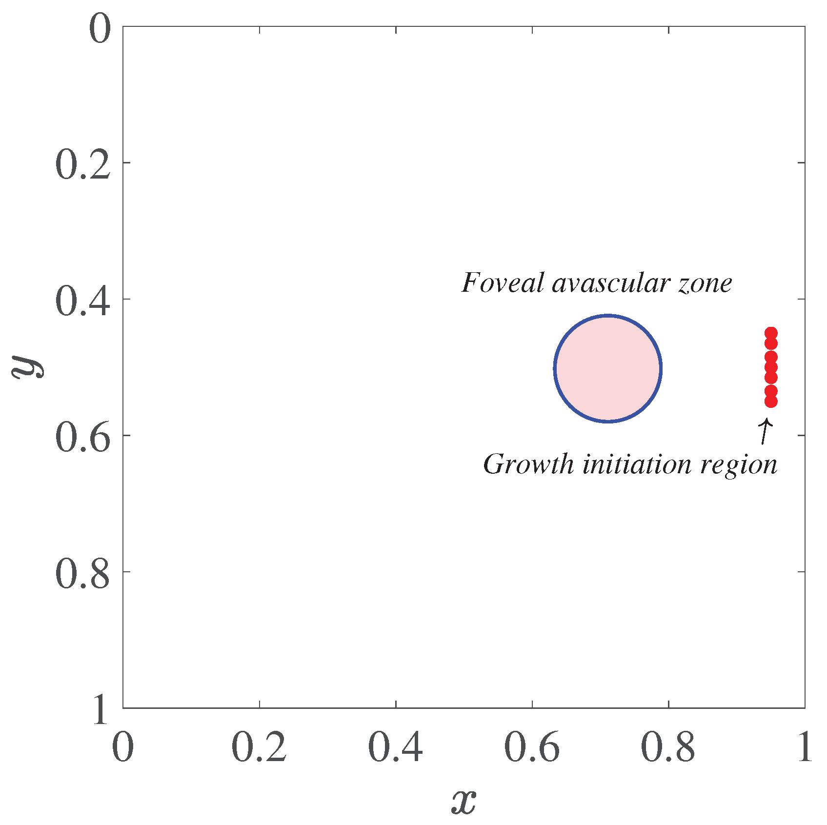
Figure 2.
Initial distributions of the angiogenic factor and fibronectin in the computational domain
Figure 2.
Initial distributions of the angiogenic factor and fibronectin in the computational domain
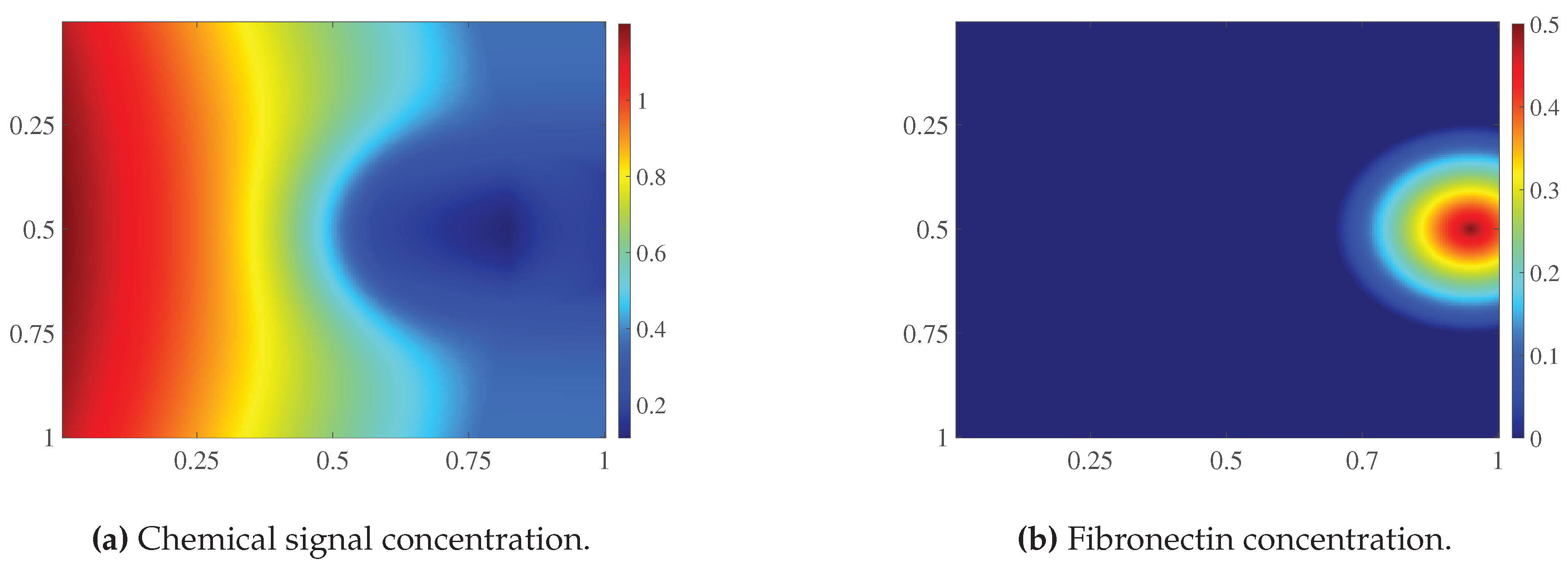
Figure 3.
Auxiliary repulsive field in the computational domain. Arrows indicate the direction of the vector . Markers denote the initial vascular tips, and the circle represents the boundary of the foveal avascular zone. Grayscale shading indicates the values of the field
Figure 3.
Auxiliary repulsive field in the computational domain. Arrows indicate the direction of the vector . Markers denote the initial vascular tips, and the circle represents the boundary of the foveal avascular zone. Grayscale shading indicates the values of the field
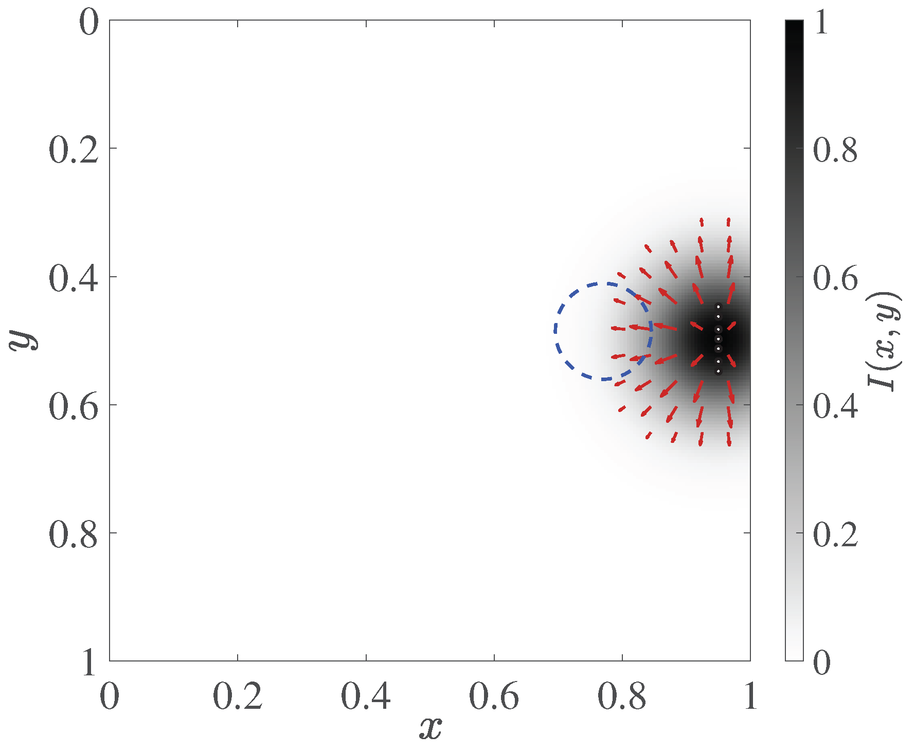
Figure 4.
Operation of the local source mechanism for and . (a) First-stage trajectories. (b) Field after small sprout initiation, before the first regular time step of the second stage. (c) Final trajectories and source states. (d) Final field after 1000 time steps of the second stage. Panels (b) and (d) use the same color scale range of . The dashed line indicates the FAZ boundary. In panel (c), black denotes first-stage trajectories, and blue denotes new trajectory nodes formed during the second stage; green circles indicate active sources, and gray crosses indicate deactivated sources. The trajectory panels show network nodes; line thickness does not encode the assigned diameters.
Figure 4.
Operation of the local source mechanism for and . (a) First-stage trajectories. (b) Field after small sprout initiation, before the first regular time step of the second stage. (c) Final trajectories and source states. (d) Final field after 1000 time steps of the second stage. Panels (b) and (d) use the same color scale range of . The dashed line indicates the FAZ boundary. In panel (c), black denotes first-stage trajectories, and blue denotes new trajectory nodes formed during the second stage; green circles indicate active sources, and gray crosses indicate deactivated sources. The trajectory panels show network nodes; line thickness does not encode the assigned diameters.
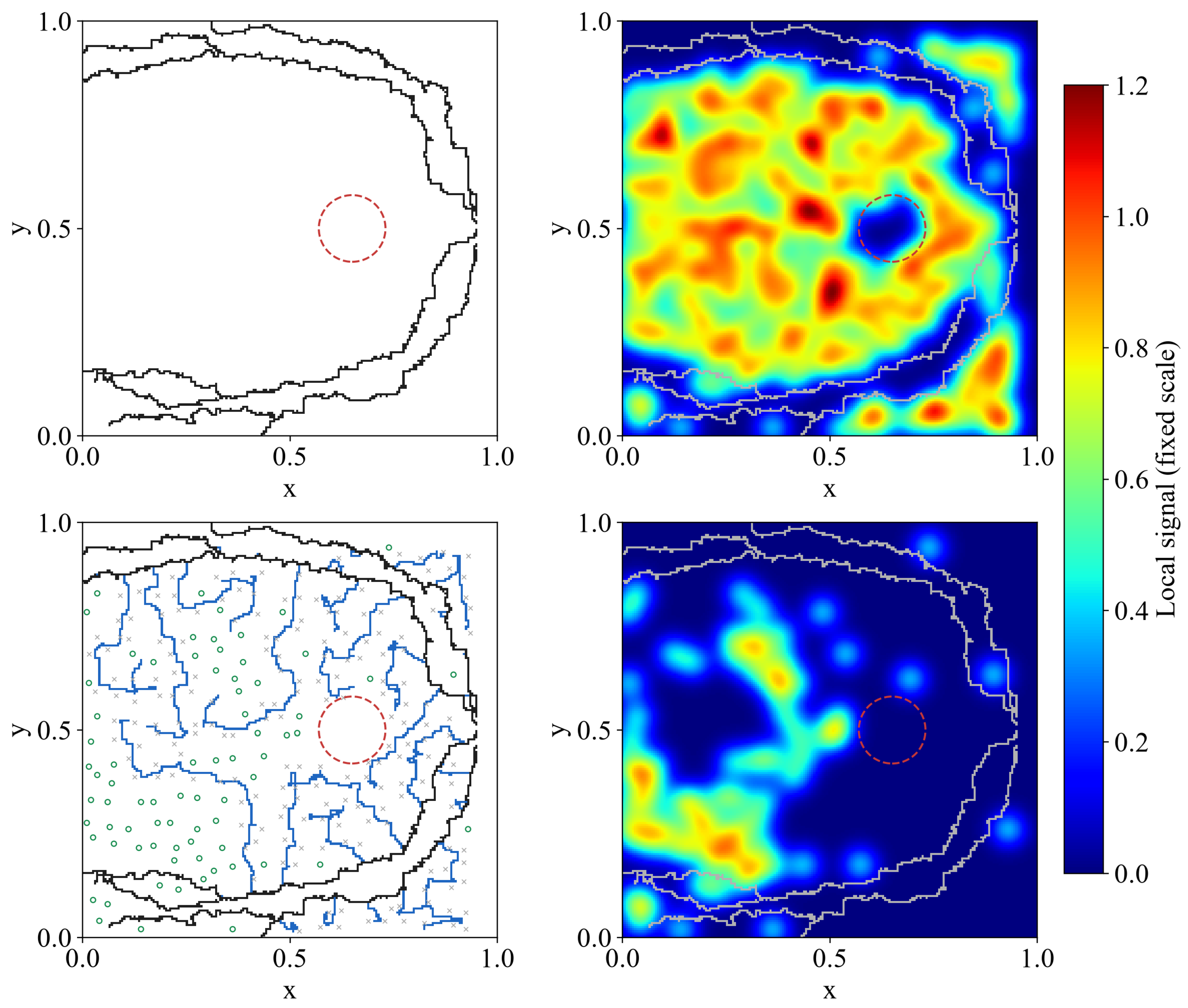
Figure 5.
Comparison of Bayesian optimization and random search using a common initial sample of 33 configurations. (a) Mean loss of each new configuration on . (b) Best mean loss attained, including the common initial sample, as a function of the number of additional simulations per method. The 99 shared initial simulations are not included on the horizontal axis of panel (b). Lower values indicate a smaller discrepancy from the reference characteristics.
Figure 5.
Comparison of Bayesian optimization and random search using a common initial sample of 33 configurations. (a) Mean loss of each new configuration on . (b) Best mean loss attained, including the common initial sample, as a function of the number of additional simulations per method. The 99 shared initial simulations are not included on the horizontal axis of panel (b). Lower values indicate a smaller discrepancy from the reference characteristics.
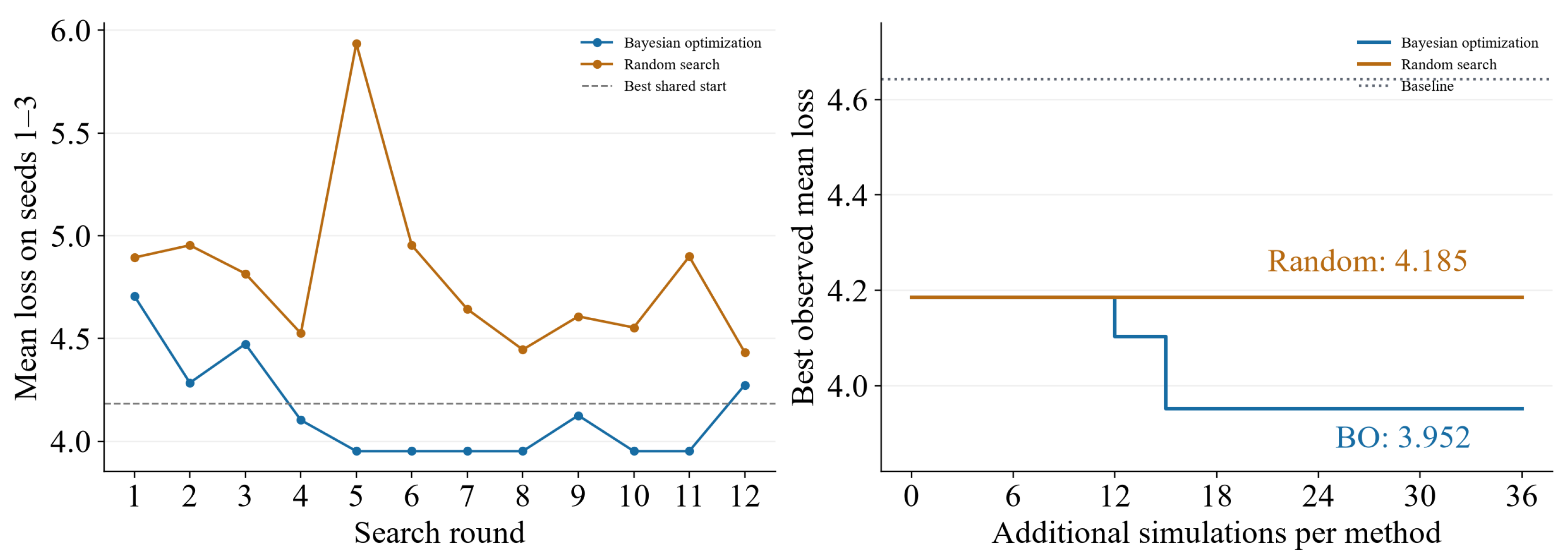
Figure 6.
Losses of three fixed configurations on new . (a) Individual values, means, and sample standard deviations; lines connect results obtained using the same seed. (b) Paired loss differences relative to the BO configuration. A positive difference indicates a lower loss for BO.
Figure 6.
Losses of three fixed configurations on new . (a) Individual values, means, and sample standard deviations; lines connect results obtained using the same seed. (b) Paired loss differences relative to the BO configuration. A positive difference indicates a lower loss for BO.
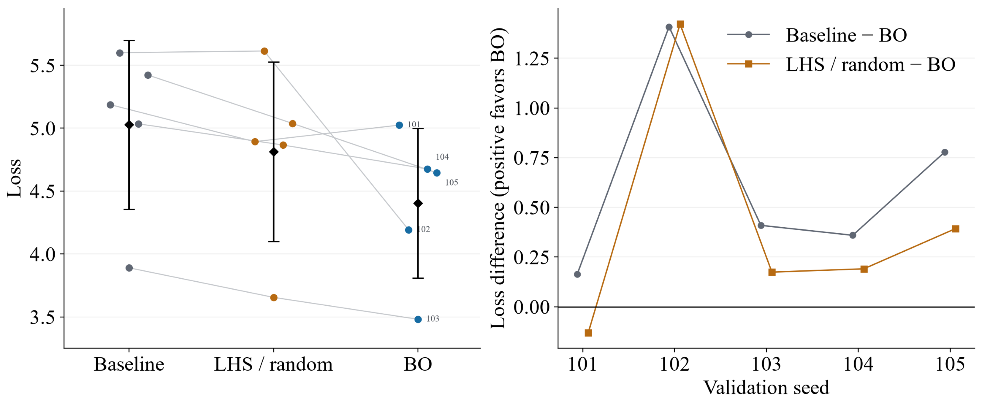
Figure 7.
Mean normalized absolute errors of six morphological features on . The target medians and normalization scales were fixed using the calibration reference masks. Lower values indicate closer agreement with the target characteristics.
Figure 7.
Mean normalized absolute errors of six morphological features on . The target medians and normalization scales were fixed using the calibration reference masks. Lower values indicate closer agreement with the target characteristics.
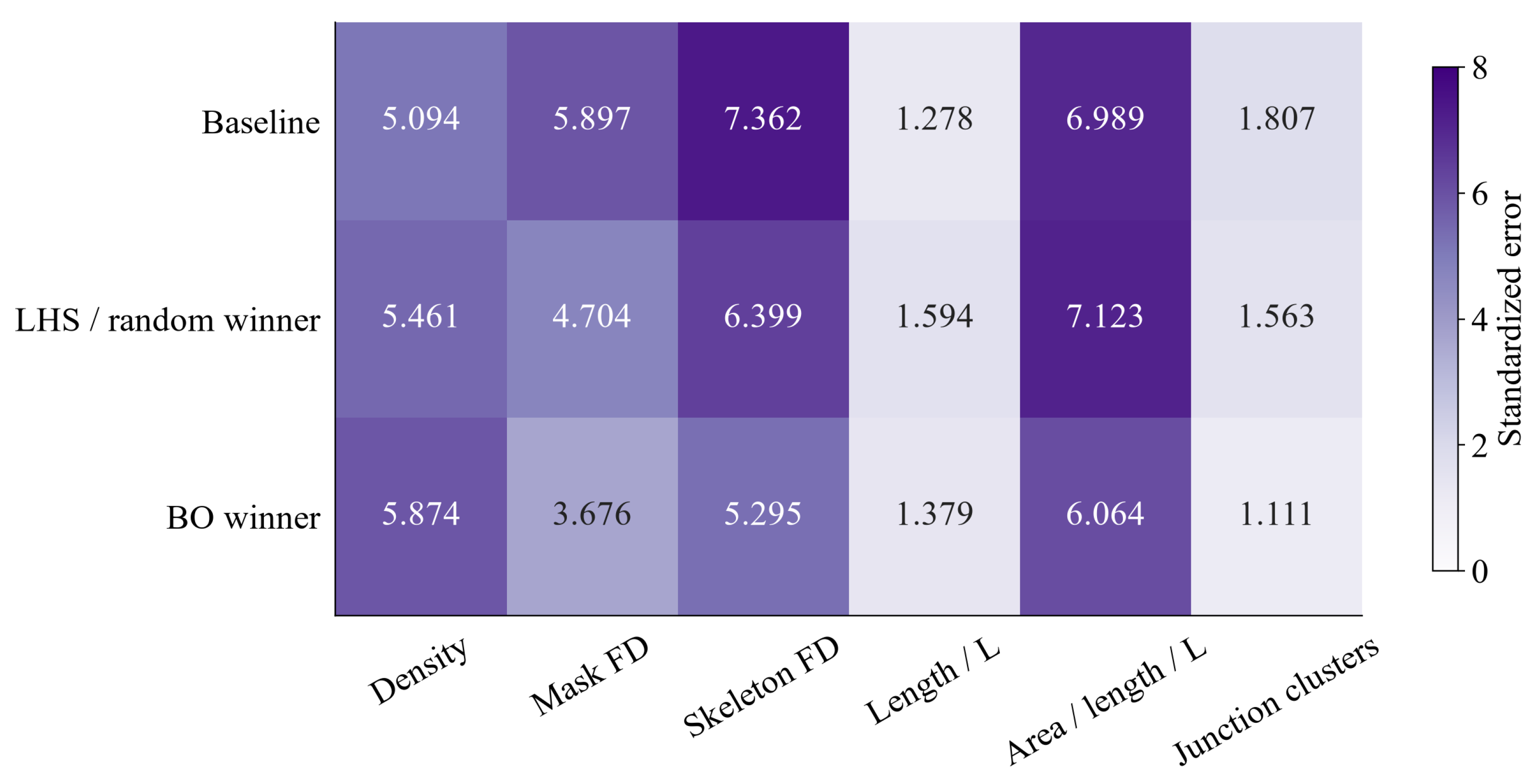
Figure 8.
Binary vascular masks for the baseline parameters, the random search result, and the BO configuration. Rows correspond to configurations, and columns correspond to the common . The individual loss J is given below each mask. All fifteen evaluation realizations are shown.
Figure 8.
Binary vascular masks for the baseline parameters, the random search result, and the BO configuration. Rows correspond to configurations, and columns correspond to the common . The individual loss J is given below each mask. All fifteen evaluation realizations are shown.
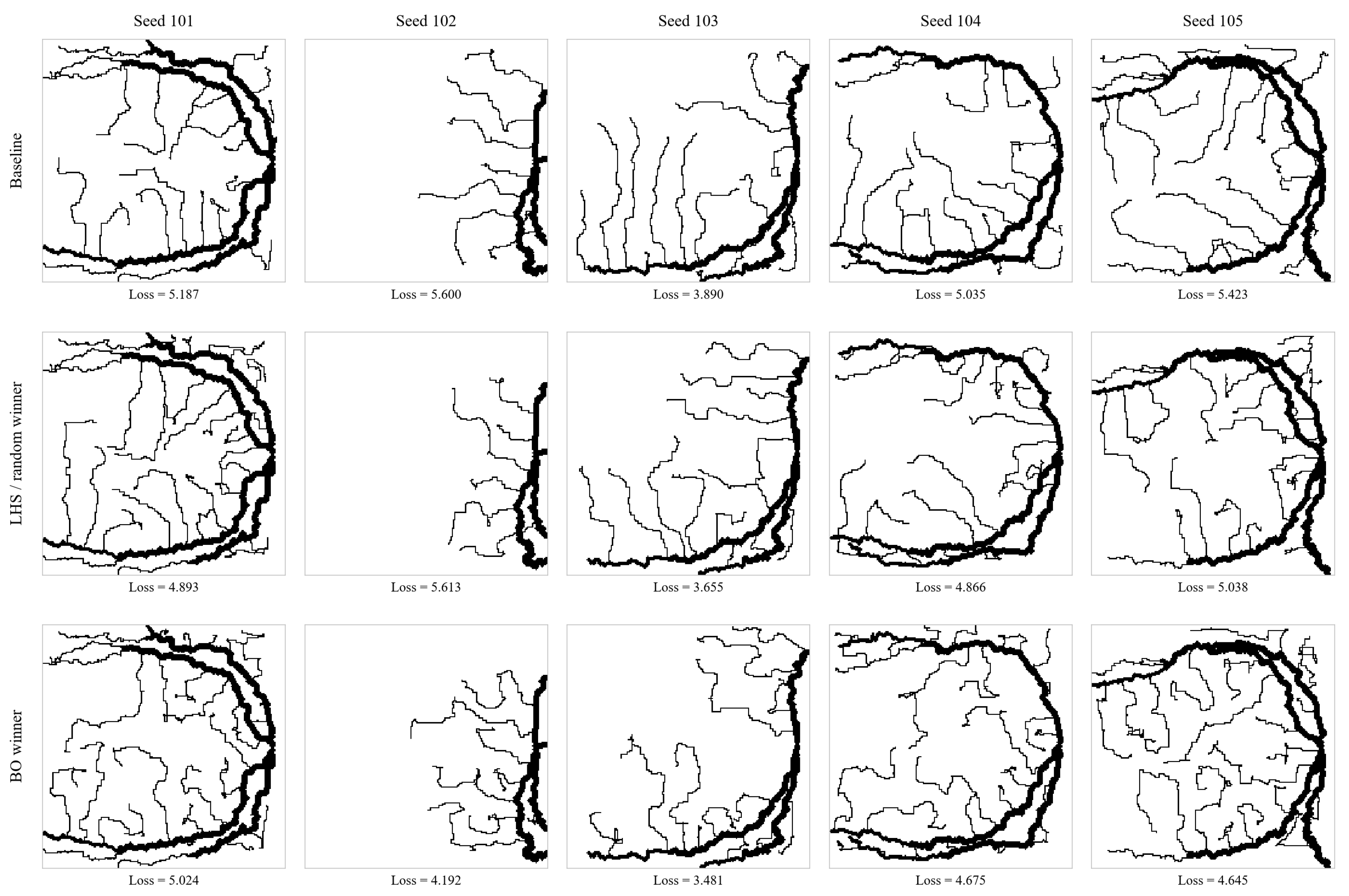

Table 1.
Second-stage parameters, search ranges, and values selected by Bayesian optimization (BO). Spatial parameters are expressed in grid spacings.
Table 1.
Second-stage parameters, search ranges, and values selected by Bayesian optimization (BO). Spatial parameters are expressed in grid spacings.
| Parameter | Range | Baseline | Selected by BO |
|---|---|---|---|
| Source spacing | 10–20 | 14 | 10 |
| Source width | 6–14 | 10 | 6 |
| Coverage radius | 4–8 | 6 | 4 |
| Requested number of sprouts | 20–40 | 30 | 40 |
Table 2.
Mean loss during parameter selection and final evaluation. Values are reported as mean ± sample standard deviation across realizations. Lower values indicate a smaller discrepancy from the reference characteristics.
Table 2.
Mean loss during parameter selection and final evaluation. Values are reported as mean ± sample standard deviation across realizations. Lower values indicate a smaller discrepancy from the reference characteristics.
| Configuration | Seeds 1–3 | Seeds 101–105 |
|---|---|---|
| Baseline parameters | ||
| Random search result | ||
| Bayesian optimization |
Table 3.
Mean normalized block errors on seeds 101–105.
| Block | Baseline | Random search | Bayesian optimization |
|---|---|---|---|
| Density | |||
| Fractal estimates | |||
| Geometry | |||
| Overall mean |
Table 4.
One-factor parameter variations relative to the baseline configuration. The modified parameter value is given in parentheses.
Table 4.
One-factor parameter variations relative to the baseline configuration. The modified parameter value is given in parentheses.
| Parameter | Decreased value: loss | Increased value: loss |
|---|---|---|
Disclaimer/Publisher’s Note: The statements, opinions and data contained in all publications are solely those of the individual author(s) and contributor(s) and not of MDPI and/or the editor(s). MDPI and/or the editor(s) disclaim responsibility for any injury to people or property resulting from any ideas, methods, instructions or products referred to in the content. |
© 2026 by the authors. Licensee MDPI, Basel, Switzerland. This article is an open access article distributed under the terms and conditions of the Creative Commons Attribution (CC BY) license (http://creativecommons.org/licenses/by/4.0/).
Copyright: This open access article is published under a Creative Commons CC BY 4.0 license, which permit the free download, distribution, and reuse, provided that the author and preprint are cited in any reuse.