

Submitted:
09 November 2026
Posted:
12 November 2026
You are already at the latest version
Abstract
Transferring a decoder trained on overt (pronounced) speech to inner speech has been proposed to offset scarce inner-speech EEG. This was re-examined on the “Thinking out loud” dataset (ds003626, 10 participants, four words), with no test trial in training or selection. EEGNet, ShallowConvNet, CSP+LDA and a Riemannian tangent-space pipeline were compared on bidirectional transfer, combined training, overt pre-training with fine-tuning on 25–100% inner-speech subsets, maximum-mean-discrepancy alignment and four trial windows. Shuffled-label controls and an exploratory, post hoc test family were used. Cross-participant, held-out-session, channel, band, external-electrode and second-dataset (ds006104) arms were reference checks. Within participant, overt speech was decodable in the action interval (0.34–0.43, chance 0.250). It survived a held-out session, peaked in 30–100 Hz and did not cross participants. Two lip electrodes alone decoded the pronounced word at 0.67–0.83. Regressing the external electrodes out of the scalp reduced three decoders’ overt accuracy to 0.28–0.40, leaving a residual of undetermined origin. Inner-speech accuracy was not distinguishable from chance. No transfer method, fine-tuned or not, improved reliably on its controls. Effects below about 2–6 percentage points were likely missed. These findings suggest that articulation-related features learned from overt speech may not provide sufficiently transferable information for inner-speech decoding under the present conditions.
Keywords:
inner speech
; imagined speech
; EEG
; transfer learning
; brain–computer interface
; data leakage
; evaluation protocol
; EEGNet
; Riemannian geometry
1. Introduction
Inner speech is the silent production of words without articulation. It is the signal that a speech brain–computer interface (BCI) [1,2] for people who cannot speak would have to read. Intracortical and electrocorticographic speech neuroprostheses now synthesise or decode attempted speech at conversational rates [3,4,5,6,7,8]. Even a completely locked-in patient has communicated through an implanted interface [9]. Several sensing routes have been proposed for silent speech interfaces [10,11]. Among them, scalp EEG is the non-invasive route most likely to make such a device widely available. Labelled inner-speech EEG is scarce, because the task is tiring and the label cannot be checked from outside. Reviews of the field agree that single-trial accuracies remain low and heterogeneous [12,13,14,15,16,17]. One idea is borrowed from transfer learning in motor-imagery BCIs [18,19,20]. A decoder is trained on overt (pronounced) speech, which is easier to collect and to verify. It is then transferred to inner speech, with or without a small calibration set. Articulated-speech EEG has been used in this way for imagined-speech decoding [21]. Intracranial work shows that overt and imagined speech share some spectrotemporal features [22,23]. Early EEG studies decoded imagined vowels and words within participant at modest rates [24,25]. On the open “Thinking out loud” dataset of Nieto et al. [26], a deep-learning baseline reached only 29.7% on four words [27]. An earlier internal analysis produced substantially higher cross-condition accuracies, but subsequent examination revealed data leakage in the evaluation protocol. The present study replaces that analysis with a leakage-controlled evaluation.
Two recent audits motivate the present study. Leakage between training and evaluation is now recognised as a general cause of over-optimistic machine-learning results across sciences [28]. Small neuroimaging samples also make the resulting error bars wide [29,30]. Brookshire et al. [31] found that most deep-learning studies of translational EEG they examined contained a form of data leakage. In those studies, accuracies fell from near-perfect to near-chance when the leak was closed. Adeika and Osuagwu [32,33] re-evaluated imagined-speech decoding on ds003626 and two other corpora under leakage-controlled splits. Cross-subject inner-speech accuracy stayed within 0.006 of chance. Adding pronounced trials to inner-speech training gave nothing. The pronounced condition itself was decoded mainly from lip and facial muscle activity, and nothing was left in the 8–30 Hz band. The same authors document three ways in which ds003626 is misread [33]. The condition codes run against the intuitive order. The class encoding changed between public releases. Condition is a deterministic function of time within a session. Our pipeline was verified against each of these (Section 2.1). The transfer question itself was not tested in those studies. It asks whether a decoder trained on overt speech under the same controls carries anything into inner speech. It also asks in which direction, in which part of the trial and with how much target calibration, and whether explicit distribution alignment helps.
This question is addressed here on ds003626 as a controlled evaluation. Two results on this dataset have already been reported by Adeika and Osuagwu [32,33]. Inner-speech decoding was at chance under leakage-controlled evaluation, and articulation-related muscle activity made a substantial contribution to overt-speech decoding. Both results are replicated here, but they are not presented as findings of this study. The contribution of this study is a systematic and controlled evaluation of cross-condition transfer learning on one harness. In this harness, every arm that reports inner-speech accuracy scores the same held-out inner-speech trials. Model selection uses a validation split that is never the test split. The pronounced and inner trial sets are checked to be disjoint. The evaluation has five parts:
- Bidirectional transfer. Overt→inner and inner→overt transfer were each compared with within-condition training and with combined training.
- Target-domain calibration and fine-tuning. Inner-speech training sets of 25, 50 and 100% were used alone and after pre-training on overt speech.
- MMD alignment re-evaluated. The maximum-mean-discrepancy penalty that accompanied the earlier, leaked transfer claim was re-run under the same controls.
- Networks against conventional pipelines. Two convolutional networks (EEGNet, ShallowConvNet) were compared with CSP+LDA and a Riemannian tangent-space pipeline in every arm.
- Temporal segmentation. Every arm was run on four windows: the full trial, the action interval in which the word is produced, the concentration-plus-cue interval and the concentration interval alone. In this way, pre-stimulus, cue-locked and speech-locked components can be told apart.
Every cell carries a shuffled-label counterpart and a 95% confidence interval over participants. Paired effect sizes are given with an approximate minimum detectable effect. An exploratory Wilcoxon test against chance and per-participant binomial thresholds [34] are also reported. Leave-one-subject-out (LOSO), held-out-session, channel-subset, band-limited (8–30 and 30–100 Hz), external-electrode and second-dataset arms are reference checks. Each was run once, so that the overt reference and the inner-speech result can be read against the two preprints rather than re-derived.
The results follow one line. Overt speech is decodable within participant in the action interval by three of the four decoders, also when the test session is held out. Inner-speech accuracy is not distinguishable from chance in any arm. None of the evaluated transfer methods improves reliably on its controls, although improvements of a few percentage points cannot be excluded. Articulation-related signals contribute substantially to overt-speech decoding. The overt signal is concentrated above 30 Hz, is not localised and is participant-specific. It is read better from two lip electrodes than from the 128 scalp channels. For the three decoders that read it above chance, it is reduced, but not removed, when the external electrodes are regressed out of the scalp. These observations offer one explanation of why overt-to-inner transfer gave no reliable gain here. All of this is stated as what these decoders found under this protocol, not as a statement about what the recordings contain. In the Discussion, it is used to say when cross-condition transfer could be expected to work.
2. Materials and Methods
2.1. Dataset
The OpenNeuro dataset ds003626, version 2.1.2, was used [26]. It contains ten healthy Spanish-speaking participants with three sessions each. EEG was recorded from 128 BioSemi channels and eight external (EXG) electrodes. Four directional words (arriba, abajo, derecha, izquierda) were produced in three conditions: pronounced (overt), inner speech and visualised. Each trial consists of a concentration interval (0.5 s), a visual cue (0.5 s), an action interval (2.5 s, 1.0–3.5 s from trial onset) and a relaxation interval. The cue is a white arrow pointing in the direction of the word.
The authors’ derivative scalp epochs were used ( to s around cue onset). They were processed separately for each participant and session. The data were re-referenced to the ear-lobe electrodes and band-pass filtered at 0.5–100 Hz with a 50 Hz notch on the continuous recording. They were then epoched, decimated to 256 Hz and cleaned by infomax independent component analysis. Components were removed by their correlation with the eye and lip electrodes [26]. The paper does not state the scope of the decomposition. Section 4.6 reports how it was established and what it implies for data independence. The condition and class of each trial were taken from the companion events table. The epoch event names were not used for this, because they do not carry the condition. The visualised condition was not used.
The eight EXG electrodes sit on the ear lobes (EXG1–2), the temples (EXG3–4), above and below the right eye (EXG5–6) and above and below the lips on the right orbicularis oris (EXG7–8) [26]. The dataset provides them as derivative epochs with the same events table as the scalp epochs. They are used only in the external-electrode arms of Section 3.5. After the authors’ artefact rejection, every participant has class-balanced trial counts in each condition (Table 1). Chance is therefore exactly 0.250 for every test set.
Label integrity. Three checks are built into the loader, following the dataset pitfalls reported by Adeika and Osuagwu [33]. First, the condition codes are read as 0 = pronounced, 1 = inner speech and 2 = visualised. This is the mapping of the dataset authors’ acquisition code and events decoder. The resulting totals, 1128 pronounced and 2236 inner-speech trials, match the corrected mapping. Second, the class codes of release 2.1.2 (0–3) are compared with the word in the epoch event name for every epoch file. Loading stops on any disagreement. This also guards against the 1–4 encoding of release 1.0.0. Third, condition is a deterministic function of position within a session, so no analysis in this paper classifies condition. Every classifier separates the four words within one condition. The order of the words within a block was randomised by the dataset authors.
2.2. Trial Windows
Four windows were cut from each epoch, relative to cue onset:
- full: to s
- action: to s, the interval in which the word is produced
- cue: to s, the concentration interval and the visual cue, before any word is produced
- concentration: to 0 s, before the cue, when the participant does not yet know the word.
The cue window is not label-free. The cue is an arrow whose direction is the class. The window therefore contains a class-specific visual stimulus and possibly a directional eye movement. It is read as a stimulus-locked sensitivity check, not as a negative control. A decoder that scores above chance there is reading the arrow, its oculomotor consequence or a preparatory component, not the word. A decoder that scores at chance there does not read the arrow with the trials available. The full window includes the cue. The concentration window is the label-free control. Nothing in it can carry the class. A decoder above chance there would be reading a confound in the harness or in the trial order, not a neural signal.
2.3. Evaluation Protocol
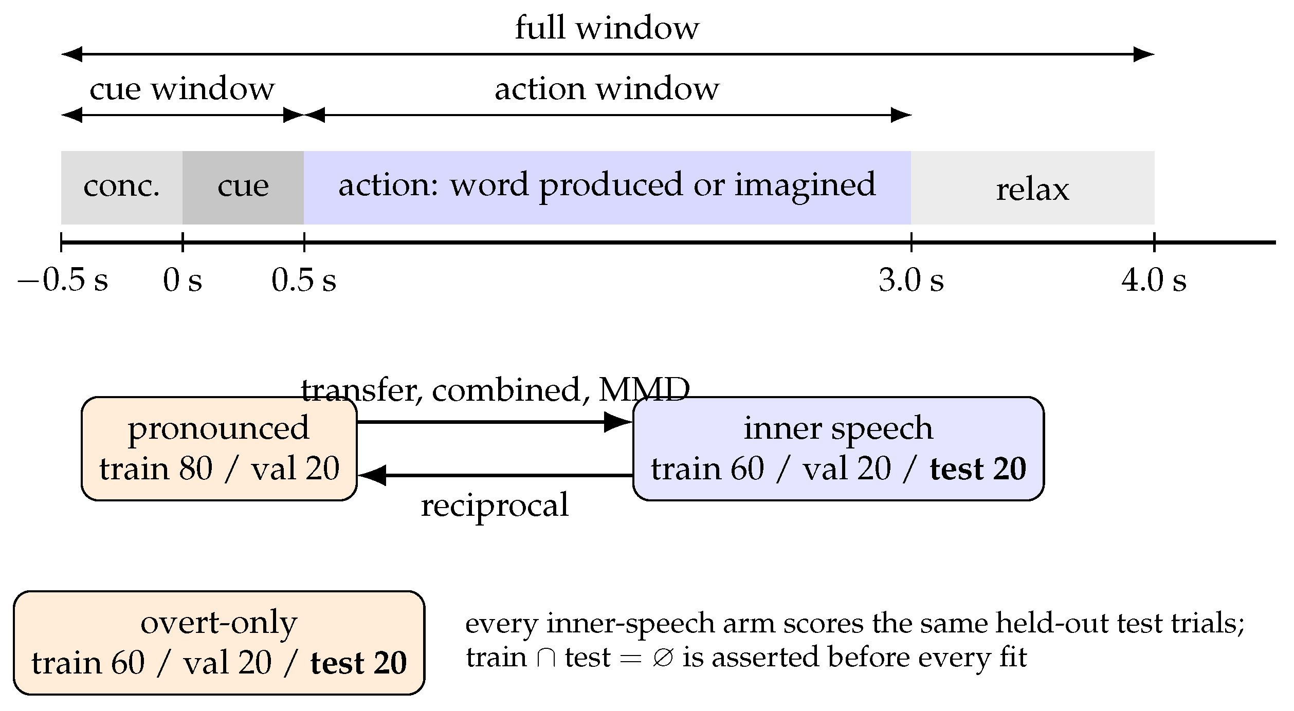
The protocol is shown in Figure 1. All splits are stratified by class and drawn once per random seed. Before any model is fitted, the sets are checked in code to share no trial.
Subject-dependent arms. For each participant and seed, the inner-speech trials were split 60/20/20 into training, validation and test sets. The pronounced trials were split 80/20 into training and validation sets. Every arm that reports an inner-speech accuracy scores the same held-out inner-speech test set. The arms are as follows.
- Target-only: training and selection on inner speech, with 25, 50 or 100% of the inner training set.
- Transfer: training and selection on pronounced speech only.
- Combined: training on the pronounced and inner training sets, selection on the inner validation set.
- MMD: as transfer, plus the alignment penalty described below.
In the reciprocal arm, the model is trained on inner speech and every pronounced trial is scored. The overt-only arm uses its own 60/20/20 split of the pronounced trials and scores held-out pronounced trials. This split is drawn from a separate random stream, so the splits of the other arms do not change. Target-only, transfer and overt-only each have a shuffled-label counterpart. In it, the training and validation labels are permuted and the test labels are left intact.
Fine-tuning arms. In the usual transfer recipe, a model is pre-trained on the source condition and then trained further on the labelled target subset. In the fine-tune arm, the network is first trained on the pronounced training set, with early stopping on the pronounced validation set. The same weights are then trained on the inner-speech training subset (25, 50 or 100%), with early stopping on the inner validation set. These are the same subsets as in the target-only arm of that seed. The held-out inner test set is then scored. The shuffled fine-tune arm permutes the pronounced training and validation labels before pre-training and changes nothing else. It shows what the same network reaches after the same fine-tuning when its pre-training carried no overt class information. Architecture, schedule and amount of pre-training are unchanged. Both arms were run only for the two networks, because the covariance pipelines have no weights to train further. Both use the optimiser, learning rate and epoch budget of every other network arm.
Held-out-session arms. The subject-dependent split pools the three recording sessions. Trials recorded minutes apart can therefore fall into training and test. A stricter within-participant reference was obtained by repeating the overt-only, inner-only, transfer, reciprocal and shuffled arms with one session held out as the test set in turn. The other two sessions were split 80/20 into training and validation, stratified by class. Each held-out session, participant and seed gives one row. The test sets then contain 20–40 pronounced and 40–80 inner-speech trials.
Arms on data rebuilt without independent component analysis. The derivative epochs were cleaned by a decomposition fitted on all trials of a session (Section 4.6). Training and test trials of a session therefore share its unmixing. To remove this dependency, every session was rebuilt from the raw recording with the fixed steps of the dataset authors only. These steps are the ear-lobe reference, a 50 Hz notch and a 0.5–100 Hz zero-phase finite-impulse-response band-pass on the continuous recording. Epochs from to s around cue onset were then cut, decimated by four and mean-removed. None of these steps estimates a parameter from the data.
The band-pass is, however, a zero-phase filter on the continuous recording. Its impulse response (6759 taps at 1024 Hz, s) is longer than the 1.7–2.1 s gap between consecutive epochs. An epoch is therefore not strictly independent of its neighbours. The size of this dependency was measured on two sessions (sub-01 ses-01 and sub-05 ses-02). Eight channels spread over the cap and 20 random trials per session were used. The in-band activity of a single trial’s window was filtered alone. It contributes a median of 0.1–0.2% (at most 0.6%) of the norm of the mean-removed epoch before or after it. This agrees with the 0.18% of the kernel’s norm that lies beyond the shortest gap. The contribution is label-free. The observed contribution was small, and the adjacent-trial word agreement was close to chance (0.234 over the 5550 adjacent pairs of all 30 sessions, against 0.250), suggesting a limited risk of class-related contamination. The derivative epochs were filtered in the same way. In the held-out-session arms, the test session is a separate recording, so the dependency cannot reach them. The measurement is reproduced by filter_spread.py in the code repository.
Trials, word codes and condition labels were taken from the derivatives and checked to match trial by trial. For one session, the rebuilt and derivative epochs differ only in a subspace of exactly the dimension that the decomposition had removed. The overt-only, inner-only, transfer, reciprocal and shuffled arms were repeated on the rebuilt data in the action window. The four decoders and seeds 0–2 were used. These seeds give the same splits as the first three seeds of Table 3.
Leave-one-subject-out arms. For each held-out participant s, the next participant in the list served as the validation participant. The remaining eight formed the training pool. Nothing from s enters training or model selection. In inner-LOSO, the model is trained on the inner speech of the pool and every inner-speech trial of s is scored. Overt-LOSO does the same with pronounced speech. In transfer-LOSO, the model is trained on the pronounced speech of the pool and the inner speech of s is scored. In shuffled inner-LOSO, the labels of the pool are permuted. The data of the held-out participant were not aligned. This is discussed in the Limitations.
Second-dataset reference arms. It was checked whether the within-participant overt result depends on the dataset. The overt-only arm, the overt-LOSO arm and their shuffled controls were run on the overt-speech dataset ds006104, version 1.0.1 [35]. It contains 16 participants recorded with 64-channel EEG. Each participant spoke 80 trials of 20 consonant–vowel syllables aloud. The syllables are /b, p, d, t/ followed by one of five vowels. Epochs ran from 0.5 s before to 0.2 s after speech onset, at 500 Hz, on the 61 scalp channels common to all participants. The 20-class syllable task (chance 0.050) was decoded across participants only, because each participant has four trials per syllable. The binary place-of-articulation and voicing tasks (chance 0.500, balanced) were decoded within participant and across participants. The within-participant split was 60/20/20, with 16 test trials. Both the broadband preprocessing of the dataset (1–40 Hz) and an 8–30 Hz band-pass were used. Unlike the ds003626 action window, this epoch ends shortly after articulation begins. An overt signal that depends on articulation is therefore expected to be weak or absent.
External-electrode arms. These arms measure directly how much of the overt reference the artefact electrodes carry. The overt-only, inner-only, transfer and shuffled arms were repeated in the action window on three signals:
- the eight EXG electrodes alone
- the lip pair (EXG7–8) alone
- the 128 scalp channels with the EXG regressed out.
The regression is fitted within each trial. Let hold the eight EXG time series of trial i and a column of ones. Scalp channel c of that trial is replaced by its least-squares residual,
Every fit uses only the samples of its own trial. No information crosses trials, so no split can leak through the regression. The regression removes the part of each scalp channel that is linearly and instantaneously mixed with what the external electrodes record. Before any split, the EXG epochs of each participant were checked to carry the same labels, conditions and sessions as the scalp epochs. The splits, decoders and normalisation are those of the subject-dependent arms with seeds 0–2. These arms therefore score the same test trials as the first three seeds of Table 3.
Normalisation. Let be the amplitude of trial i, channel c and sample t. Each channel was z-scored with the mean and standard deviation of that channel over all trials and samples of the training set of the arm. In LOSO, these were pooled over the training participants. The same transform was applied to validation and test trials:
where is the set of training trials and T the number of samples in the window. Test statistics therefore never enter the normalisation.
Band-limited variants. For the 8–30 Hz and 30–100 Hz arms, a fourth-order Butterworth band-pass was applied forward and backward (zero phase) to every trial before normalisation. Sensorimotor rhythms lie in the 8–30 Hz band [36]. Adeika and Osuagwu report that none of the overt signal lies there [33]. Scalp electromyography has most of its power in the 30–100 Hz band [37,38].
Figure 1.
Trial structure of ds003626, the four windows and the subject-dependent splits. The concentration window is the first half of the cue window. Pronounced and inner-speech trial sets are disjoint by construction. The held-out inner-speech fifth is never seen by training or model selection in any arm. The leave-one-subject-out arms hold out one participant entirely and select models on a second participant.
Figure 1.
Trial structure of ds003626, the four windows and the subject-dependent splits. The concentration window is the first half of the cue window. Pronounced and inner-speech trial sets are disjoint by construction. The held-out inner-speech fifth is never seen by training or model selection in any arm. The leave-one-subject-out arms hold out one participant entirely and select models on a second participant.
2.4. Decoders
Networks. Two compact convolutional networks were used. Both are widely used in EEG decoding [39,40], and both were compared with other network families for EEG speech classification in our earlier work [41]. The first is EEGNet [42] (, , temporal kernel 64, dropout 0.5). The second is ShallowConvNet [43] (40 temporal and spatial filters, filter length 25, square–mean-pool–log, dropout 0.5). Both were trained with Adam (learning rate , weight decay ) and batch size 32. Training ran for up to 100 epochs with early stopping on validation accuracy (patience 15). The parameters of the best validation epoch were restored before testing. Five seeds (0–4) were run for the subject-dependent broadband arms. Three seeds (0–2) were run for the LOSO, held-out-session, channel-subset and band-limited arms. Every table states its seed count.
Hyperparameters were set to the published defaults of each architecture and were not tuned on this dataset. Tuning on the data that is later reported is the practice this study argues against. As a result, the networks may be under-tuned. The seed-to-seed variance reported with each result is the measure of this. Early stopping used the 20% validation split of the arm, which holds only 20–48 trials per participant. The shuffled-label counterparts show what selection on such a split alone can produce. The layers and parameter counts are listed in Table 2. Both networks are small relative to the 100–240 training trials per participant. The number of parameters changes with the window only through the input size of the classifier.
Classical pipelines. For each normalised trial ( channels), a shrunk sample covariance was computed with the oracle-approximating shrinkage estimator [44],
with the closed-form OAS shrinkage intensity.
In the CSP+LDA pipeline, common spatial patterns [45] are computed in the multiclass form of Grosse-Wentrup and Buss [46], as implemented in pyRiemann. They yield spatial filters from the training covariances. Each trial is represented by its log-variance features
These features are classified by linear discriminant analysis with Ledoit–Wolf shrinkage of its covariance [47]. CSP+LDA has been the reference pipeline of BCI classification reviews for a decade [48,49].
In the Riemannian pipeline, is the affine-invariant Riemannian mean of the training covariances. Each trial is mapped to the tangent space at [50,51,52],
where vectorises the upper triangle with off-diagonal entries weighted by . The vector is classified by -regularised multinomial logistic regression with .
The grid value ( or C) was chosen on the validation split of each arm. The mean and the filters are estimated from training trials only. Both pipelines (scikit-learn [53] and pyRiemann) ran on the same normalised trials and splits as the networks, with three seeds.
MMD alignment. Let denote the penultimate-layer (flattened) features of the network. In the MMD arm, two random batches were drawn at every optimisation step. One holds m pronounced training trials , and the other holds n unlabelled inner-speech training trials . The loss was
where is the cross-entropy on the pronounced batch. The kernel is Gaussian, . Its bandwidth h is the median pairwise squared distance within the joint batch. The batch sizes were , and [54]. The target trials contribute no labels. The model was selected on the pronounced validation set, so the inner-speech test set remains unseen. The weight reproduces the setting of our earlier analysis.
2.5. Channel Subsets
The overt-only and inner-only arms (EEGNet, action window, three seeds) were repeated on 12 channel conditions:
- all 128 electrodes
- a three-electrode left primary motor strip (nearest BioSemi positions to C5, C3, C1) and its right-hemisphere mirror
- a nine-electrode left sensorimotor set (FC5, FC3, FC1, C5, C3, C1, CP5, CP3, CP1) and its right-hemisphere mirror
- a 16-electrode peripheral ring on the frontal, temporal and occipital rim, where articulation EMG enters scalp EEG
- three random draws each of three and nine electrodes.
Ten-ten labels were mapped to the nearest BioSemi 128 electrode by three-dimensional distance, using the standard montages of MNE-Python [55]. The electrodes of every subset are listed in Appendix C.
2.6. Statistics
For each cell (window, model, arm, calibration fraction), the accuracy of participant p is the mean over seeds. The mean over the participants is reported with its 95% t-interval,
where is the standard deviation of the . Three further quantities are reported. The first is a one-sided Wilcoxon signed-rank test [56] of the against 0.250. It is Holm-corrected [57] over a family of M cells. The ordered p-values are replaced by
The second is the number of participants with . The third is the number of participants whose exceeds their own binomial threshold for their test-set size [34],
A participant is counted as above threshold when . The thresholds are as follows:
- 0.400–0.417 for the subject-dependent overt test sets (20–24 trials)
- 0.354–0.375 for the subject-dependent inner test sets (36–48 trials)
- 0.375–0.400 for the held-out-session pronounced sets (20–40 trials) and 0.325–0.375 for the inner sets (40–80 trials)
- 0.317–0.324 for the LOSO pronounced sets (100–120 trials) and 0.296–0.306 for the LOSO inner sets (180–240 trials).
The tables report the largest threshold in each cell. On the second dataset, the thresholds are 0.688 for the 16-trial within-participant sets. They are 0.588 (binary) or 0.087 (20-class) for the 80-trial LOSO sets. The thresholds are calibrated for a single split, whereas is a mean over seeds, so the count is conservative. A cell is read as positive only if its shuffled counterpart is at chance.
Test family. With , the smallest one-sided exact Wilcoxon p is . A Holm family of 126 cells, as in Appendix A, therefore has a floor of and can never reach . The corrected values of such a family are descriptive. The primary family was therefore designated after the full table was available, on the basis of the study question. It consists of the 12 cells of the action window that answer the question of the paper: overt-only, inner-only (100%) and transfer for each of the four decoders. Its floor is . It includes the arms that failed, but it was not pre-registered. The statistical analysis of this paper is therefore exploratory, not confirmatory. Corrected p values quoted in the text refer to this family unless a table states its own, and they are descriptive. The reading rests on effect sizes with their intervals, on the shuffled controls and on the per-participant counts.
The held-out-session and band-limited tables are corrected within their own 24 cells. The concentration-window table is corrected within its 42 cells. The external-electrode table is corrected within its 72 cells. Its floor of lies above , so its corrected values are descriptive. Its reading rests on the shuffled controls and the per-participant counts. Arms that score the same held-out trials are compared by their paired per-participant differences, with effect sizes and detectable effects (below), and by their shuffled counterparts. The paper asks two between-arm questions. The first is whether fine-tuning improves on training from scratch at the same calibration fraction. The second is whether regressing the external electrodes out lowers the overt accuracy of each decoder. Both are answered by one-sided Wilcoxon tests of the paired per-participant difference. These are Holm-corrected over six cells (two networks, three fractions) and four cells (four decoders), respectively.
Effect sizes and detectable effects. For the comparisons that answer the transfer question, each arm is paired with its control participant by participant on the same test trials. The mean difference in percentage points is reported with its 95% t-interval. Next to it, the smallest difference the design could detect is reported. It is computed for a one-sided test at with 80% power, from the observed spread of the paired differences:
This formula uses the t approximation. The MDE is therefore an approximate reference for the size of effect the design could resolve. It is not an exact threshold for statistical significance under the tests actually used. The exact Wilcoxon test has slightly less power than the t test. The Holm correction raises the threshold further within each family. The effect needed to reach a corrected with the same power is therefore larger than the MDE. Throughout the paper, detectable effects are meant in this approximate sense.
Reading a null. A cell is called “not distinguishable from chance” when its 95% interval covers 0.250. A comparison is called “no reliable improvement” when its paired interval covers zero or its effect does not survive correction. Neither phrase means that the effect is absent. The upper bound of the interval is the largest effect the cell leaves open. It is quoted with the null so that the resolution of each statement is explicit.
2.7. Code and Compute
All code is in the project repository. The software versions were Python 3.11.15, PyTorch 2.11.0 with CUDA 12.8 and NVIDIA driver 581.57, MNE-Python 1.12.1, scikit-learn 1.9.0, pyRiemann 0.12, NumPy 2.4.6 and SciPy 1.17.1. Every arm asserts that its training and test trials are disjoint before fitting. Every result row records the split sizes and the seed. Runs resume from per-participant result files. Network arms ran on one NVIDIA RTX 5070 Ti, and classical arms ran on CPU. Two runs of the same configuration in this paper differ by 2.5 percentage points. These are the all-channel EEGNet overt-only cell with three and five seeds. This is the run-to-run variance that should be attached to any single network number here.
3. Results
The results are presented in five steps. First, overt speech is decodable within participant (Section 3.1). Second, inner speech is not distinguishable from chance, and no transfer method improves reliably on its controls (Section 3.2). Third, the overt signal does not cross participants, is not localised and is concentrated above 30 Hz (Section 3.3 and Section 3.4). Fourth, a large part of it is accounted for by articulation-related signals recorded by the external electrodes (Section 3.5). Fifth, no overt signal is found in a second overt dataset epoched up to speech onset (Section 3.6).
3.1. Overt Speech Is Decodable Within Participant in the Action Interval
The subject-dependent results in the action window are given in Table 3. Every cell of the full, action and cue windows is listed in Appendix A (Table A1). Held-out pronounced trials were decoded above chance by three of the four decoders: Riemannian 0.432 (95% CI 0.367–0.497), EEGNet 0.367 (0.304–0.430) and ShallowConvNet 0.340 (0.289–0.391). CSP+LDA reached 0.273 (0.228–0.318), which is above chance numerically only. For CSP+LDA, six of ten participants were above chance, none was above threshold, and the uncorrected p was 0.21. For Riemannian and EEGNet, ten of ten participants were above chance. Four and two of them, respectively, were above their individual binomial threshold. The shuffled-label overt controls were at chance (0.229–0.259).
In the 12-cell primary family, the Holm-corrected p of the overt cells was for Riemannian and EEGNet, for ShallowConvNet and for CSP+LDA. Over the 126 cells of Appendix A, the same cells are at the family floor of . For this reason, that correction is reported as descriptive. In the cue window, which contains the arrow, overt accuracy was not distinguishable from chance for any model (0.197–0.273). In the full window it was intermediate (0.279–0.338). The strongest overt decoder was the covariance-based Riemannian pipeline, not a network.

Table 3.
Subject-dependent accuracy in the action window, mean over ten participants [95% t-CI], with the number of participants above chance (0.250) and above their own binomial threshold. Target calibration fraction 1.0 unless stated. Shuffled-label counterparts in italics. Holm-corrected p values for every cell are in Table A1.
Table 3.
Subject-dependent accuracy in the action window, mean over ten participants [95% t-CI], with the number of participants above chance (0.250) and above their own binomial threshold. Target calibration fraction 1.0 unless stated. Shuffled-label counterparts in italics. Holm-corrected p values for every cell are in Table A1.
| Arm | EEGNet | ShallowConvNet | CSP+LDA | Riemannian |
|---|---|---|---|---|
| Overt-only (pron.→pron.) | 0.367 [0.304, 0.430]; 10, 2 | 0.340 [0.289, 0.391]; 9, 2 | 0.273 [0.228, 0.318]; 6, 0 | 0.432 [0.367, 0.497]; 10, 4 |
| shuffled overt | 0.242 | 0.259 | 0.229 | 0.246 |
| Inner-only (inner→inner) | 0.241 [0.225, 0.256]; 2, 0 | 0.254 [0.233, 0.276]; 5, 0 | 0.226 [0.184, 0.268]; 4, 0 | 0.211 [0.184, 0.239]; 2, 0 |
| shuffled inner | 0.260 | 0.258 | 0.259 | 0.271 |
| 50% calibration | 0.248 | 0.254 | 0.239 | 0.208 |
| 25% calibration | 0.252 | 0.249 | 0.238 | 0.221 |
| Transfer (pron.→inner) | 0.248 [0.234, 0.263]; 3, 0 | 0.253 [0.239, 0.268]; 5, 0 | 0.284 [0.253, 0.315]; 9, 0 | 0.259 [0.237, 0.281]; 5, 0 |
| shuffled transfer | 0.253 | 0.256 | 0.233 | 0.236 |
| Transfer + MMD | 0.248 [0.233, 0.264]; 4, 0 | 0.252 [0.235, 0.269]; 5, 0 | – | – |
| Combined (pron.+inner→inner) | 0.266 [0.245, 0.287]; 7, 0 | 0.250 [0.226, 0.274]; 4, 0 | 0.234 [0.208, 0.260]; 3, 0 | 0.221 [0.199, 0.243]; 2, 0 |
| Reciprocal (inner→pron.) | 0.252 [0.233, 0.270]; 4, 0 | 0.254 [0.239, 0.269]; 6, 0 | 0.255 [0.236, 0.274]; 5, 0 | 0.267 [0.245, 0.289]; 7, 0 |
Concentration window. Every arm on the 0.5 s before the cue, when the participant does not yet know the word, is given in Table A2 (Appendix B). Nothing was read by any decoder. Overt-only accuracy was 0.194–0.269, inner-only 0.199–0.254, transfer 0.258–0.269, reciprocal 0.241–0.258 and combined 0.210–0.273. The shuffled controls were at 0.222–0.268. No participant was above threshold in any of the 42 cells of the window (Holm-corrected ). Two cells are below 0.05 before correction. The first is EEGNet combined training (0.273, 0.258–0.288), with nine of ten participants above 0.250 and an uncorrected p of 0.003. The second is ShallowConvNet with MMD (0.266, ). Both are of the size of the cue-window group effects, and neither is an overt-only or inner-only cell. The harness therefore finds nothing in a label-free interval. This indicates that the cue-window effects are locked to the stimulus and are not carried by the trial order. In the overt-only and inner-only cells, the Riemannian pipeline scored below chance (0.194, 0.165–0.223, and 0.199, 0.183–0.215), with no participant above 0.250. Its shuffled controls were at chance. This is discussed in the Limitations.
Without independent component analysis. The key arms were repeated on the epochs rebuilt from the raw recordings, in which no step is fitted across trials (Table 4). The inner-speech and transfer cells stayed at chance. Inner-only accuracy was 0.218–0.260, transfer 0.252–0.275 and reciprocal 0.245–0.268. The shuffled controls were at 0.237–0.266. No participant was above threshold except one Riemannian reciprocal participant. Against the same seeds on the derivatives, the paired differences were to points. They were not consistent across participants: three to eight of ten were higher, with two-sided . The CSP+LDA transfer cell had shown a positive paired trend on the derivatives. Here it was 0.275, against a shuffled control of 0.259.
Overt accuracy rose for every decoder, by 11 to 22 points. Riemannian reached 0.600 (0.507–0.692), with ten of ten participants above chance and nine above threshold. ShallowConvNet reached 0.560 (0.460–0.659; ten and nine), EEGNet 0.492 (0.396–0.587; ten and five) and CSP+LDA 0.386 (0.295–0.478; eight and four). Accuracy was higher than on the derivatives in eight to ten of ten participants. The shuffled overt controls were at 0.237–0.253. The decomposition had removed components correlated with the eye and lip electrodes. This rise is therefore what the articulation account predicts. The inner-speech and transfer results do not depend on it.
Held-out session. The within-participant arms were repeated with one recording session held out (Table 5). The overt reference remained above chance but was smaller. Riemannian reached 0.384 (0.327–0.442), with ten of ten participants above chance and five above threshold (Holm over the 24 cells of the table). EEGNet reached 0.319 (0.286–0.353; ten and one; ). CSP+LDA reached 0.280 (0.253–0.307; eight and none; ) and ShallowConvNet 0.277 (0.236–0.317; six and none; ). The shuffled overt controls were at 0.247–0.257. None of the null arms changed. Inner-only accuracy was 0.247–0.256, transfer 0.250–0.255 and reciprocal 0.242–0.267. Each was inside the interval of its shuffled counterpart. In this paper, the held-out-session numbers are taken as the within-participant overt reference. The pooled-session numbers of Table 3 are taken as their upper bound.
3.2. Inner Speech Is Not Distinguishable from Chance, and No Transfer Method Improves Reliably
The inner-only arm was not distinguishable from chance for any model or training fraction (0.208–0.254, upper 95% bounds 0.239–0.276; Table 3). It was inside the interval of its shuffled-label counterpart (0.258–0.271). Under the pooled-session split, the two covariance pipelines were below 0.250 on inner speech. For example, Riemannian inner-only accuracy was 0.184–0.221 across windows, with zero to two participants above chance. This disappears under the held-out-session protocol, where the same Riemannian cell is 0.254 (0.244–0.264) in Table 5. The below-chance values are therefore a property of the pooled split, in which trials of one session fall into both training and test. They are not a property of inner speech and are not interpreted further. On the same held-out inner trials, the transfer arm scored 0.248–0.284 across models. The reciprocal arm scored 0.252–0.267 on pronounced trials, and the combined arm 0.221–0.266. No participant crossed a binomial threshold in any of these arms.
Paired effects. Each transfer arm was paired with its controls on the same test trials (Table 6). For the two networks, transfer differed from inner-only training and from the shuffled-transfer control by to percentage points. The intervals were about to points, and the detectable effects were 1.6–3.5 points. Fine-tuning after overt pre-training differed from inner-only training at the same fraction by to points (detectable effects 2.6–4.1, Holm over the six cells). It differed from pre-training on permuted overt labels by to points (Holm ).
Positive differences were found for the covariance pipelines. CSP+LDA transfer exceeded inner-only training by 5.8 points (0.9–10.8) and its shuffled control by 5.1 (0.8–9.3). Riemannian transfer exceeded them by 4.8 (0.7–8.8) and 2.2 (–4.6). The uncorrected one-sided p was 0.014–0.042, and the Holm-corrected p was over these eight comparisons. No participant was above threshold. Part of the difference against inner-only training comes from inner-only accuracy below 0.250 for these pipelines (0.226 and 0.211), not from transfer above it (0.284 and 0.259). Under the held-out-session protocol, the same transfer arms were 0.254 and 0.250 (Table 5). Every transfer comparison is therefore read as no reliable improvement. It is not read as evidence that transfer has no effect. Gains of up to about 2–3 points for the networks and up to 9–11 points for the covariance pipelines lie inside the intervals.
The overt cells are read in the same way. Their evidence is the per-participant consistency, the shuffled control and the replication across protocols, not the corrected p value alone.
The cue window contains the arrow but no word. In this window, EEGNet scored 0.26–0.29 in every arm. This includes inner-only (0.276), transfer (0.269), reciprocal (0.286, two participants above threshold), combined (0.285, none) and the shuffled transfer control (0.257). The Holm-corrected p was over the appendix family. This is read as a small stimulus-locked component shared by all arms, not as inner-speech information. It is consistent with the arrow being weakly readable by this network. None of it is seen in the action window.
Adding the MMD penalty produced no reliable change. Accuracy was 0.248 (EEGNet) and 0.252 (ShallowConvNet) in the action window, 0.265 and 0.263 in the cue window, and 0.258 and 0.248 in the full window. Each value was within two points of the plain transfer arm and of the shuffled transfer control (Figure 2). Aligning the feature distributions of pronounced and inner trials did not produce a reliable gain on inner speech.
Fine-tuning. Pre-training on pronounced speech and then continuing on the inner-speech subset did not reliably improve on training from scratch either (Table 7). The fine-tune arm scored 0.249–0.268 across the two networks and three fractions. Training from scratch on the same subsets scored 0.236–0.258, and pre-training on shuffled pronounced labels 0.240–0.257. Every fine-tune interval but one covered 0.250. The exception was ShallowConvNet at 50% (0.267 [0.251, 0.283]). Its Holm-corrected p was 0.72 over the 18 cells of the table, and no participant was above threshold. The paired per-participant gain of fine-tuning over training from scratch was +0.3 to +3.2 points. Five to seven of ten participants were positive. The smallest uncorrected one-sided p was 0.038, and the Holm-corrected p over the six cells was . Over shuffled pre-training, the gain was to +2.6 points (smallest uncorrected p 0.014, corrected 0.084). Any contribution of the pronounced pre-training is within three points and is not distinguishable from pre-training on permuted labels.
3.3. The Overt Signal Does Not Cross Participants
The leave-one-subject-out results in the action window are given in Table 8 and Figure 3. Here the held-out participant was kept out of training and model selection. Overt-LOSO fell to 0.245–0.263 for the four models. Inner-LOSO was 0.243–0.259, transfer-LOSO 0.244–0.260 and the shuffled inner-LOSO control 0.245–0.252. Every Holm-corrected p was . The overt-LOSO and transfer-LOSO arms contain 80 participant–model pairs. Two of them crossed their binomial threshold (0.30–0.32 for these test sizes). The first was Riemannian overt-LOSO for participant 03 (0.370). The second was CSP+LDA transfer-LOSO for participant 10 (0.308, three trials above its threshold of 0.296). The other 78 did not, and no network pair did in any arm. The contrast per participant is shown in Figure 4. Of the 40 points, 34 lie below the diagonal. The CSP+LDA points lie on both sides of it, near chance. Only the one Riemannian point rises above the LOSO threshold band.
3.4. The Overt Signal Is Not Spatially Specific and Is Concentrated Above 30 Hz
EEGNet overt-only accuracy across the 12 channel conditions is shown in Figure 5a. All 128 electrodes gave 0.342. The three random nine-electrode draws gave 0.336–0.366, and the 16-electrode peripheral ring gave 0.326. The left C5/C3/C1 strip gave 0.315, and the nine-electrode left sensorimotor set 0.305. Three random electrodes gave 0.296–0.312, and the right-hemisphere mirrors 0.292–0.315. Inner-only accuracy was not distinguishable from chance in any set (0.231–0.273). The signal was read as well from three random electrodes or the peripheral rim as from the left speech-motor strip. It is therefore not localised to the cortex that produces speech.
When every trial was restricted to 8–30 Hz (Figure 5b, Table 10), the overt signal was lost for both networks. EEGNet fell from 0.367 to 0.238 (one participant above chance), and ShallowConvNet from 0.340 to 0.249 (four). A reduced overt signal was kept in this band by the covariance-based pipelines. Riemannian reached 0.330 (0.272–0.389), with nine participants above chance and two above threshold (uncorrected , Holm over the 24 cells). CSP+LDA reached 0.324 (0.249–0.399; seven and two; Holm ). Their shuffled controls were at 0.231 and 0.242. Inner-only (0.229–0.251) and transfer (0.242–0.270) remained not distinguishable from chance in this band. The one transfer cell that rose numerically (EEGNet, 0.270) was matched by its own shuffled control (0.263).
The opposite was found when every trial was restricted to 30–100 Hz (Table 9, Figure 5b). Every decoder read the pronounced condition better than with the broadband signal. CSP+LDA rose from 0.273 to 0.536 (0.408–0.664), with ten of ten participants above chance and six above threshold (Holm over the 24 cells). Riemannian rose from 0.432 to 0.535 (0.395–0.675; nine and six; ). EEGNet rose from 0.367 to 0.439 (0.330–0.548; ten and four; ), and ShallowConvNet from 0.340 to 0.420 (0.337–0.503; ten and four; ). The shuffled overt controls were at 0.233–0.255. Inner-only (0.200–0.254), transfer (0.250–0.261) and reciprocal (0.244–0.263) remained inside the intervals of their shuffled counterparts. The overt signal used by these decoders is therefore concentrated above 30 Hz, where scalp electromyography has most of its power. The 8–30 Hz residual of the covariance pipelines is the smaller part of it.
Table 9.
Subject-dependent accuracy in the action window after a 30–100 Hz band-pass (three seeds). Values are means over ten participants [95% t-CI], followed by the number of participants above chance and above their binomial threshold. Broadband value in parentheses. Holm correction over the 24 cells of this table.
Table 9.
Subject-dependent accuracy in the action window after a 30–100 Hz band-pass (three seeds). Values are means over ten participants [95% t-CI], followed by the number of participants above chance and above their binomial threshold. Broadband value in parentheses. Holm correction over the 24 cells of this table.
| Arm | EEGNet | ShallowConvNet | CSP+LDA | Riemannian |
|---|---|---|---|---|
| Overt-only | 0.439 [0.330, 0.548]; 10, 4 (0.367) | 0.420 [0.337, 0.503]; 10, 4 (0.340) | 0.536 [0.408, 0.664]; 10, 6 (0.273) | 0.535 [0.395, 0.675]; 9, 6 (0.432) |
| shuffled overt | 0.251 | 0.255 | 0.233 | 0.254 |
| Inner-only | 0.254 [0.239, 0.269]; 7, 0 | 0.247 [0.226, 0.268]; 4, 0 | 0.216 [0.176, 0.256]; 3, 0 | 0.200 [0.175, 0.225]; 0, 0 |
| Transfer | 0.250 [0.228, 0.272]; 3, 0 | 0.259 [0.236, 0.283]; 7, 0 | 0.261 [0.246, 0.275]; 7, 0 | 0.260 [0.246, 0.275]; 8, 0 |
| shuffled transfer | 0.259 | 0.246 | 0.241 | 0.235 |
| Reciprocal | 0.249 [0.230, 0.268]; 5, 0 | 0.257 [0.232, 0.282]; 5, 0 | 0.244 [0.226, 0.261]; 3, 0 | 0.263 [0.242, 0.283]; 7, 1 |
Table 10.
Subject-dependent accuracy in the action window after an 8–30 Hz band-pass (three seeds). Values are means over ten participants [95% t-CI], followed by the number of participants above chance. Holm-corrected over the 24 cells of this table. Broadband value in parentheses.
Table 10.
Subject-dependent accuracy in the action window after an 8–30 Hz band-pass (three seeds). Values are means over ten participants [95% t-CI], followed by the number of participants above chance. Holm-corrected over the 24 cells of this table. Broadband value in parentheses.
| Arm | EEGNet | ShallowConvNet | CSP+LDA | Riemannian |
|---|---|---|---|---|
| Overt-only | 0.238 [0.216, 0.259]; 1 (0.367) | 0.249 [0.215, 0.282]; 4 (0.340) | 0.324 [0.249, 0.399]; 7 (0.273) | 0.330 [0.272, 0.389]; 9 (0.432) |
| shuffled overt | 0.233 | 0.231 | 0.242 | 0.231 |
| Inner-only | 0.251 [0.234, 0.268]; 5 | 0.240 [0.217, 0.262]; 4 | 0.229 [0.196, 0.263]; 4 | 0.231 [0.208, 0.253]; 3 |
| Transfer | 0.270 [0.241, 0.298]; 6 | 0.242 [0.227, 0.256]; 3 | 0.245 [0.217, 0.273]; 3 | 0.244 [0.229, 0.260]; 3 |
| shuffled transfer | 0.263 | 0.237 | 0.248 | 0.259 |
| Reciprocal | 0.239 [0.227, 0.250]; 2 | 0.248 [0.232, 0.264]; 5 | 0.252 [0.226, 0.278]; 4 | 0.266 [0.247, 0.284]; 6 |
3.5. The Lip Electrodes Alone Read the Pronounced Word Better than the Scalp
The action-window arms on the external electrodes and on the regressed scalp are given in Table 11. From the eight EXG electrodes alone, every decoder read the pronounced word far above any scalp result. Riemannian reached 0.902 (0.829–0.975), ShallowConvNet 0.813 (0.691–0.935), CSP+LDA 0.794 (0.693–0.896) and EEGNet 0.659 (0.538–0.781). In every cell, ten of ten participants were above chance. Ten (nine for EEGNet) were above their binomial threshold. The lip pair alone gave 0.668–0.826, with ten of ten participants above threshold for every decoder. Even the least decodable participant reached 0.417–0.517, depending on the decoder. The shuffled overt controls on both signals were at chance (0.224–0.276).
The eight external electrodes were then regressed out of every scalp trial. This reduced the overt signal of both networks until no participant remained above threshold. EEGNet reached 0.304 (0.272–0.336), with nine of ten participants above chance and none above threshold. This is a paired drop of 5.0 points from the broadband value on the same three seeds (0.354), seen in seven of ten participants (one-sided , Holm over the four decoders). ShallowConvNet reached 0.279 (0.243–0.315; seven and none). This is a drop of 5.6 points from 0.336, seen in nine of ten participants (, Holm 0.020). Most of the signal was kept by the Riemannian pipeline. It reached 0.402 (0.335–0.468), with ten participants above chance and four above threshold, as before regression. This is a drop of 3.0 points, seen in eight of ten participants (, Holm 0.17). CSP+LDA had been at 0.273 and was 0.306 after regression (0.239–0.374; seven and two).
Inner-only (0.212–0.262) and transfer (0.237–0.271) were not distinguishable from chance on any of the three signals. Their upper bounds were at most 0.297, inside the range of their shuffled controls (0.235–0.269). No participant was above threshold, except one in the ShallowConvNet transfer cell on the EXG signal. The lip electrodes thus carry information about the pronounced word. No such information was detected from them in the inner-speech condition. Measured against chance, the regression removed about half of the networks’ above-chance overt accuracy. For EEGNet it went from 10.4 to 5.4 points, and for ShallowConvNet from 8.6 to 2.9. It removed about one sixth of the Riemannian pipeline’s (18.2 to 15.2). The source of what remains cannot be determined with these data (Section 4.1).
3.6. A Second Overt Dataset, Epoched up to Speech Onset, Gives No Overt Signal
On ds006104, no overt information was found within participant by any of the four decoders (Table A3, Appendix B). With the broadband signal, place of articulation was decoded at 0.443–0.501 and voicing at 0.473–0.527. At 8–30 Hz, accuracy was 0.473–0.499. The shuffled controls were in the same range (0.484–0.516). No participant was above the 16-trial threshold of 0.688, except one EEGNet voicing participant. Across participants, place (0.475–0.537), voicing (0.483–0.520) and the 20-class syllable task (0.045–0.056) were also within the range of their shuffled controls. No participant exceeded the 80-trial threshold. One of the 80 cells differs at the group level and is reported so that it is not over-read. This is ShallowConvNet overt-LOSO on place with the broadband signal: 0.537 [0.526, 0.549], with all 16 participants above 0.500. Its Holm-corrected p was 0.017 over the 80 cells of this family, against a shuffled control of 0.484. Its best participant reached 0.583, below threshold, and the same cell at 8–30 Hz was 0.528 (Holm ). It is read as a small, consistent group effect of about four points, not as a second overt reference. The epochs of this dataset cover the pre-speech interval and the first 200 ms of articulation. In them, these decoders found no overt-speech signal within participant and none that crosses participants. This is consistent with the articulation account of the ds003626 overt result, although it is not a test of it.
4. Discussion
4.1. What the Overt Result Is, and What It Is Not
The pronounced condition was read above chance within participant by three of the four decoders. The Riemannian tangent-space pipeline read it best. The reference was reduced, but it remained when the test session was held out (0.384 and 0.319 for the two decoders that kept ten of ten participants above chance). Four observations are consistent with a substantial contribution of articulation-related activity [37,38,58]. None of them excludes a cortical speech-motor contribution [59]. The amount of signal carried by the artefact electrodes was then measured in the external-electrode arms. First, the signal was present only while the word was being produced. The arrow in the cue interval was not read by any decoder, and nothing was read in the concentration interval before it. Second, the signal was as strong from three random electrodes or the peripheral rim as from the left motor strip. This would not be expected from a sensorimotor source. Third, the signal did not generalise to held-out participants beyond a single one, although electrode positions and task were identical. In contrast, cross-participant decoding of sensorimotor rhythms is routinely above chance even before alignment [18,60,61]. Fourth, for every decoder the signal was strongest in 30–100 Hz, where scalp electromyography has most of its power. The networks found nothing in 8–30 Hz.
The measurement is given in Table 11. The pronounced word was decoded at 0.67–0.83 from the two lip electrodes alone and at 0.66–0.90 from the eight external electrodes. This is about twice the best scalp decoder. It held although scalp components correlated with the lip electrodes had already been removed by the dataset authors’ independent component analysis. When the eight channels were regressed out of every scalp trial, about half of the networks’ above-chance overt accuracy was removed (0.35 to 0.30 and 0.34 to 0.28 on the same seeds, no participant left above threshold). About one sixth of the Riemannian pipeline’s was removed (0.43 to 0.40, four participants still above threshold). CSP+LDA read overt speech only weakly before regression (0.273). It scored 0.306 after it, inside its interval (0.239–0.374), so for that decoder regression made no measurable difference. The same reading was reached on this dataset by Adeika and Osuagwu [33] from the lip electrodes alone, and it is reproduced here with four decoders.
What the regression leaves is the open point. Within-trial least squares removes only the part of a scalp channel that is linearly and instantaneously mixed with the signals of the eight external electrodes. Several sources stay in the residual. These are electromyography from muscles the electrodes do not sample (temporalis, masseter, neck, tongue), glossokinetic potentials, the auditory response to the participant’s own voice and volume-conducted cortical activity in the gamma range. The 8–30 Hz component also stays. In this band, both low-frequency muscle activity [37,38] and sensorimotor desynchronisation during articulation [36] are expected. The residual signal is largest for the Riemannian pipeline. It is compatible with any of these sources, and its origin cannot be determined from the present experiments. Articulation-related activity therefore contributes substantially to the overt reference. However, these results do not show that the overt decoders rely on it exclusively. Nor do they show that overt and inner speech share no neural representation. A shared component smaller than the detectable effects, or one that these decoders do not read, is compatible with every number here. The pronounced condition is therefore reported as a positive reference contaminated by articulation. It is not reported as evidence that overt speech is decodable from cortex with this montage. The same confound is faced and named in recent scalp-EEG overt-speech decoding work [62].
The second dataset narrows this reading but does not settle it. On ds006104 the epoch ends 200 ms after speech onset. There, no overt information was found within participant by the same four decoders. Across participants, none was found apart from one small group-level cell. The ds003626 overt signal therefore does not carry over to a window that contains little articulation. This is what the articulation account predicts. However, the window is not the only difference between the two datasets. Montage, language, task, trial count and preprocessing also differ. The comparison is therefore a reference check and not a controlled test.
4.2. When Cross-Condition Transfer Can Work, and Why It Did Not Here
The arms of this study separate the conditions under which an overt-to-inner transfer could succeed. A decoder transfers when the feature learned on the source condition is also class-discriminative in the target condition. Calibration data can then re-weight that feature, and alignment can remove a shift in its distribution. Each of these three mechanisms was tested here. None produced a reliable improvement over its control.
The transfer arm gives no evidence that the overt feature is discriminative on inner speech. The reciprocal arm gives no evidence that a feature learned on inner speech is discriminative on overt speech. The null is therefore symmetric and not a matter of direction. The combined arm, the three training fractions and the fine-tuning arm show no reliable change when labelled inner trials are added before or after pre-training on overt speech. This is expected when the inner-only arm itself is not distinguishable from chance. In that case these decoders have no target feature for calibration to re-weight. Pre-training on true overt labels also did not do reliably better than pre-training on permuted ones. The MMD arm shows no gain from matching the marginal feature distributions of the two conditions. This is consistent with alignment being able to move a feature but not to create a class separation that the target does not carry.
The small positive transfer differences of the covariance pipelines (Table 6) are the one place where a modest effect remains open. They shrink to chance when the test session is held out. The cue window shows what a component shared by the conditions looks like. It is a small stimulus-locked effect of similar size in every arm, including the shuffled control. The concentration window precedes the stimulus and shows none of it. These findings suggest that articulation-related features learned from overt speech may not provide sufficiently transferable information for inner-speech decoding under the present experimental conditions. They do not show that transfer cannot succeed in other settings. Such settings include more participants or trials, other decoders, a tuned fine-tuning schedule or recordings with less articulation in the source condition. A testable prediction follows. Transfer should appear only once a within-participant inner-speech signal is itself demonstrated. It should also appear only for features shared by the two conditions, such as the 8–30 Hz sensorimotor residual if it turns out to be cortical.
4.3. Why Earlier Transfer Claims, Including Ours, Did Not Survive
Overt-to-inner transfer far above chance was reported on this dataset in our earlier analysis. In that analysis the condition was taken from the epoch event names, which do not encode it. The “inner-speech” test trials were therefore pronounced trials that had also been used for training. This failure is prevented by the present harness. The condition is taken from the events table, and the pronounced and inner sets are asserted to be disjoint. Every arm that reports an inner-speech number scores one fixed held-out set. Under these conditions, no reliable improvement over the controls is shown by the transfer arm, the reciprocal arm, combined training, three calibration fractions, fine-tuning or MMD alignment. The same was found in the cue-window and full-window versions. This agrees with what the leakage audits predict [31]. The quantity that transferred before was the test set.
4.4. Relation to Adeika and Osuagwu, and What This Study Adds
Two findings of this paper are not new. Chance-level inner-speech decoding under leakage-controlled evaluation was first reported on this dataset by Adeika and Osuagwu. They also first reported a substantial articulation-related contribution to overt decoding. Our results replicate both findings. Our inner-LOSO null and the absence of benefit from adding pronounced trials replicate their leakage-controlled findings [32]. This was done with different code, different decoders and a different within-participant split. Three of our results agree with their positive-control study [33]. These are the channel results, the loss of the network overt signal in 8–30 Hz and the decoding of the pronounced condition from the lip electrodes alone. There are two points of difference, both discussed above. One is the residual 8–30 Hz overt signal of our covariance pipelines, which they did not observe. The other is the part of the Riemannian overt signal that survives regression of the external electrodes.
The present study adds a systematic, controlled evaluation of cross-condition transfer learning. This was not addressed in those studies. It consists of the following parts:
- bidirectional overt→inner and inner→overt transfer, compared with within-condition and combined training
- target-domain calibration with 25–100% of the inner-speech training set, and fine-tuning after overt pre-training with a permuted-label pre-training control
- maximum-mean-discrepancy alignment, re-evaluated under leakage control
- two networks compared with CSP+LDA and a Riemannian pipeline in every arm
- temporal segmentation into full, action, cue and pre-cue windows.
All arms were scored on identical held-out trials with paired effect sizes. In their within-participant evaluation, a held-out recording session was included next to pooled cross-validation. Both are reported here (Table 3 and Table 5). The comparison shows that the overt reference is inflated by five to ten percentage points by the pooled split. Every inner-speech and transfer number is left where it was. Their 30–100 Hz observation is also reproduced here with four decoders rather than one. Their dataset pitfalls [33] were used as the checklist against which Section 2.1 was written.
4.5. Recommendations
The following minimum is suggested for a transfer claim on scalp-EEG inner speech:
- a condition label taken from a source that actually carries it, checked against the acquisition code
- a fixed held-out target test set scored by every arm, with model selection on a separate validation set
- shuffled-label counterparts of the source-only, target-only and transfer arms
- a pre-stimulus negative control taken from an interval that contains no class-specific stimulus
- a held-out-session and a leave-one-subject-out version of the same arms
- a small, pre-specified family for the corrected test, with the rest reported descriptively
- per-participant binomial thresholds alongside group tests
- a band-limited or channel-restricted check of any overt or source-condition result before it is used as a reference, with decoding from the artefact electrodes alone and from the scalp with them regressed out where the recording includes them.
4.6. Limitations
The main study uses one dataset with ten participants and four classes. The second dataset is used only as a reference check of the overt result. It has a different window, task and montage, and it has no inner-speech condition.
Statistical power is limited by the ten participants. With the observed spread, the approximate minimum detectable effects of the paired comparisons are about 1.6–3.5 percentage points for the networks and 2.9–5.9 points for the covariance pipelines before correction (Equation 10, Table 6). Smaller effects would usually be missed. The upper 95% bounds of the inner-only arms are 0.239–0.276 in the action window and up to 0.30 in the cue window. The per-participant binomial thresholds flag only effects of ten points or more. What any corrected family can show is also capped by the smallest exact Wilcoxon p with ten participants (Section 2.6). Effects of a few percentage points, in inner-speech decoding or in transfer, are therefore not excluded by this study.
The fine-tuning arm used the optimiser, learning rate and epoch budget of training from scratch. It was run for the two networks only. A schedule tuned for transfer, or partial freezing of layers, was not explored. The Riemannian pipeline scored below chance in the overt-only and inner-only cells of the concentration window, with intervals excluding 0.250. In the action window, the same below-chance inner-only cell disappeared when the test session was held out. This points to the pooled-session split. However, the concentration window was not run under that protocol, so the mechanism there is not confirmed.
The external-electrode arms remove only what the eight electrodes record, linearly and within trial. Muscle that those electrodes do not sample stays in the residual, as does any non-linear or lagged coupling. The overt signal that survives regression is largest for the Riemannian pipeline. With this montage, it cannot be assigned to cortex or to unsampled muscle. Euclidean alignment [60,61] and Riemannian re-centring [20] were not applied to the held-out participant in the LOSO arms. They should be tried in the overt-LOSO arm, where a within-participant signal exists. The MMD weight was taken from the earlier analysis and was not swept. The MMD null is therefore a null at that setting.
The dataset paper does not state how its independent component analysis was fitted. This can be seen from the released epochs. The EEG of every one of the 30 sessions is rank-deficient by 2–15 dimensions. Any 20 trials of a session span the same reduced space as all of its trials. Two sessions of one participant together are of full rank. This pattern is produced by one decomposition per session, fitted across all trials of that session and followed by component removal. It agrees with the preprocessing code published by the authors. In that code, the decomposition is fitted once per session on all its epochs, and components are removed by their correlation with the external electrodes. The decomposition step is, however, switched off in the current version of that code. No labels enter these steps, so class information cannot be placed into the data by them. However, the unmixing and the choice of removed components are estimated from trials that later fall into both our training and our test sets. They are also estimated from pronounced and inner-speech trials together. This label-free dependency between training and test data is inherited by every user of the derivatives. It cannot be undone downstream, and its effect on our numbers is not known.
The filtering was applied to the continuous recording of each session, and no parameters are estimated from the data. Its zero-phase impulse response is longer than the gap between trials, so neighbouring epochs are not strictly independent. The measured contribution is 0.1–0.2% of an epoch’s norm, and the adjacent-trial word agreement was close to chance, suggesting a limited risk of class-related contamination (Section 2.3). The key arms were therefore repeated on epochs rebuilt from the raw recordings, with no step fitted across trials (Table 4). The inner-speech, transfer and reciprocal results were unchanged, and only the overt reference rose. The conclusions of this paper therefore do not rest on that dependency. The rebuilt data were used for this check only. All other tables use the derivatives.
5. Conclusions
On ds003626, every inner-speech test trial was kept out of training and model selection. Under this evaluation, overt speech was decodable within participant in the action interval by two convolutional networks and the Riemannian tangent-space pipeline. This also held when the test session was held out. The signal was participant-specific, spatially non-specific and concentrated above 30 Hz. The two lip electrodes alone decoded the pronounced word better than any scalp decoder. Regressing the external electrodes out of the scalp reduced, but did not remove, the overt accuracy of the two networks and the Riemannian pipeline. The weak CSP+LDA overt result stayed unchanged within its interval. Inner-speech accuracy was not distinguishable from chance for any decoder, window, band, signal or protocol. None of the evaluated transfer methods showed a reliable improvement over its controls. This applies to both directions, to combined training, to 25–100% of the inner-speech training set, to fine-tuning after overt pre-training and to maximum-mean-discrepancy alignment. With ten participants, improvements smaller than about 2–6 percentage points would probably not have been detected (an approximate bound). These findings suggest that articulation-related features learned from overt speech may not provide sufficiently transferable information for inner-speech decoding under the present conditions. They do not show that inner speech carries no decodable information or that cross-condition transfer is impossible. The conclusions are limited to one dataset of ten participants and four words. They are also limited to data whose artefact correction was estimated across all trials of a session, although the key results were unchanged on data rebuilt without it. Finally, they are limited to the four decoders and the protocols evaluated here. The positive transfer result of our own earlier analysis on this dataset is better explained by evaluation leakage than by a shared representation of overt and inner speech. The arms and controls used here are offered as a checklist for future claims.
Author Contributions
Conceptualization, K.P.P.S. and T.S.; methodology, K.P.P.S.; software, K.P.P.S.; validation, K.P.P.S.; formal analysis, K.P.P.S.; writing—original draft preparation, K.P.P.S.; writing—review and editing, T.S.; supervision, T.S. All authors have read and agreed to the published version of the manuscript.
Funding
This research received no external funding.
Institutional Review Board Statement
Not applicable; the study analysed a public, anonymised dataset.
Informed Consent Statement
Not applicable.
Data Availability Statement
The EEG data are available on OpenNeuro as dataset ds003626, version 2.1.2 (https://doi.org/10.18112/openneuro.ds003626.v2.1.2). The second dataset is OpenNeuro ds006104, version 1.0.1 [35]. The analysis code, per-participant results, figure scripts and a reproduction guide are in the GitHub repository https://github.com/lillianphyo/inner-speech-cross-condition-transfer (MIT licence), archived as release v1.0.1 on Zenodo (https://doi.org/10.5281/zenodo.23717046).
Acknowledgments
The authors thank Nieto et al. for making the dataset public.
Conflicts of Interest
The authors declare no conflict of interest.
Appendix A. Full Subject-Dependent Results
Table A1.
Every cell of the subject-dependent evaluation (Table 3 shows the action-window subset). Mean accuracy over ten participants with 95% t-CI; p, one-sided Wilcoxon against 0.250; , Holm-corrected over the 126 cells; , participants above chance; , the largest per-participant binomial threshold in the cell; , participants above their own threshold. Calibration fraction shown for inner-only only.
Table A1.
Every cell of the subject-dependent evaluation (Table 3 shows the action-window subset). Mean accuracy over ten participants with 95% t-CI; p, one-sided Wilcoxon against 0.250; , Holm-corrected over the 126 cells; , participants above chance; , the largest per-participant binomial threshold in the cell; , participants above their own threshold. Calibration fraction shown for inner-only only.
| Window | Model | Arm | Frac. | Mean [95% CI] | p | ||||
| full | EEGNet | overt-only | 0.338 [0.30, 0.37] | 0.002 | 0.24 | 9 | 0.417 | 0 | |
| full | EEGNet | shuffled overt | 0.246 [0.23, 0.27] | 0.523 | 1.00 | 4 | 0.417 | 0 | |
| full | EEGNet | inner-only | 0.25 | 0.261 [0.24, 0.28] | 0.213 | 1.00 | 5 | 0.375 | 0 |
| full | EEGNet | inner-only | 0.50 | 0.250 [0.23, 0.27] | 0.541 | 1.00 | 3 | 0.375 | 0 |
| full | EEGNet | inner-only | 1.00 | 0.252 [0.23, 0.27] | 0.461 | 1.00 | 6 | 0.375 | 0 |
| full | EEGNet | shuffled inner | 0.267 [0.25, 0.29] | 0.037 | 1.00 | 6 | 0.375 | 0 | |
| full | EEGNet | transfer | 0.261 [0.24, 0.28] | 0.209 | 1.00 | 6 | 0.375 | 0 | |
| full | EEGNet | shuffled transfer | 0.259 [0.23, 0.29] | 0.367 | 1.00 | 5 | 0.375 | 0 | |
| full | EEGNet | transfer + MMD | 0.258 [0.24, 0.27] | 0.156 | 1.00 | 7 | 0.375 | 0 | |
| full | EEGNet | combined | 0.269 [0.24, 0.29] | 0.064 | 1.00 | 6 | 0.375 | 0 | |
| full | EEGNet | reciprocal | 0.267 [0.25, 0.29] | 0.062 | 1.00 | 6 | 0.324 | 0 | |
| full | ShallowConvNet | overt-only | 0.305 [0.27, 0.34] | 0.010 | 1.00 | 7 | 0.417 | 0 | |
| full | ShallowConvNet | shuffled overt | 0.244 [0.22, 0.27] | 0.727 | 1.00 | 3 | 0.417 | 0 | |
| full | ShallowConvNet | inner-only | 0.25 | 0.252 [0.23, 0.28] | 0.652 | 1.00 | 4 | 0.375 | 0 |
| full | ShallowConvNet | inner-only | 0.50 | 0.254 [0.22, 0.28] | 0.410 | 1.00 | 4 | 0.375 | 0 |
| full | ShallowConvNet | inner-only | 1.00 | 0.246 [0.22, 0.27] | 0.688 | 1.00 | 4 | 0.375 | 0 |
| full | ShallowConvNet | shuffled inner | 0.258 [0.24, 0.27] | 0.169 | 1.00 | 5 | 0.375 | 0 | |
| full | ShallowConvNet | transfer | 0.265 [0.24, 0.30] | 0.161 | 1.00 | 6 | 0.375 | 0 | |
| full | ShallowConvNet | shuffled transfer | 0.258 [0.24, 0.28] | 0.132 | 1.00 | 6 | 0.375 | 0 | |
| full | ShallowConvNet | transfer + MMD | 0.248 [0.22, 0.27] | 0.633 | 1.00 | 4 | 0.375 | 0 | |
| full | ShallowConvNet | combined | 0.268 [0.24, 0.29] | 0.125 | 1.00 | 5 | 0.375 | 0 | |
| full | ShallowConvNet | reciprocal | 0.258 [0.24, 0.28] | 0.188 | 1.00 | 6 | 0.324 | 0 | |
| full | CSP+LDA | overt-only | 0.279 [0.21, 0.34] | 0.100 | 1.00 | 7 | 0.417 | 1 | |
| full | CSP+LDA | shuffled overt | 0.252 [0.21, 0.30] | 0.623 | 1.00 | 4 | 0.417 | 0 | |
| full | CSP+LDA | inner-only | 0.25 | 0.244 [0.22, 0.27] | 0.777 | 1.00 | 3 | 0.375 | 0 |
| full | CSP+LDA | inner-only | 0.50 | 0.243 [0.21, 0.27] | 0.731 | 1.00 | 4 | 0.375 | 0 |
| full | CSP+LDA | inner-only | 1.00 | 0.234 [0.21, 0.26] | 0.938 | 1.00 | 3 | 0.375 | 0 |
| full | CSP+LDA | shuffled inner | 0.264 [0.23, 0.30] | 0.181 | 1.00 | 5 | 0.375 | 0 | |
| full | CSP+LDA | transfer | 0.251 [0.23, 0.27] | 0.623 | 1.00 | 4 | 0.375 | 0 | |
| full | CSP+LDA | shuffled transfer | 0.231 [0.21, 0.25] | 0.981 | 1.00 | 1 | 0.375 | 0 | |
| full | CSP+LDA | combined | 0.233 [0.21, 0.26] | 0.884 | 1.00 | 5 | 0.375 | 0 | |
| full | CSP+LDA | reciprocal | 0.260 [0.24, 0.28] | 0.161 | 1.00 | 6 | 0.324 | 0 | |
| full | Riemannian | overt-only | 0.320 [0.27, 0.37] | 0.008 | 0.94 | 7 | 0.417 | 1 | |
| full | Riemannian | shuffled overt | 0.234 [0.19, 0.28] | 0.723 | 1.00 | 4 | 0.417 | 0 | |
| full | Riemannian | inner-only | 0.25 | 0.218 [0.19, 0.24] | 0.986 | 1.00 | 2 | 0.375 | 0 |
| full | Riemannian | inner-only | 0.50 | 0.203 [0.18, 0.23] | 1.000 | 1.00 | 0 | 0.375 | 0 |
| full | Riemannian | inner-only | 1.00 | 0.184 [0.16, 0.21] | 0.999 | 1.00 | 1 | 0.375 | 0 |
| full | Riemannian | shuffled inner | 0.268 [0.24, 0.29] | 0.080 | 1.00 | 8 | 0.375 | 0 | |
| full | Riemannian | transfer | 0.247 [0.22, 0.27] | 0.674 | 1.00 | 4 | 0.375 | 0 | |
| full | Riemannian | shuffled transfer | 0.236 [0.21, 0.26] | 0.839 | 1.00 | 4 | 0.375 | 0 | |
| full | Riemannian | combined | 0.206 [0.19, 0.22] | 1.000 | 1.00 | 0 | 0.375 | 0 | |
| full | Riemannian | reciprocal | 0.263 [0.25, 0.27] | 0.019 | 1.00 | 8 | 0.324 | 0 | |
| action | EEGNet | overt-only | 0.367 [0.30, 0.43] | 0.001 | 0.12 | 10 | 0.417 | 2 | |
| action | EEGNet | shuffled overt | 0.242 [0.21, 0.27] | 0.742 | 1.00 | 4 | 0.417 | 0 | |
| action | EEGNet | inner-only | 0.25 | 0.252 [0.24, 0.26] | 0.473 | 1.00 | 4 | 0.375 | 0 |
| action | EEGNet | inner-only | 0.50 | 0.248 [0.24, 0.26] | 0.662 | 1.00 | 3 | 0.375 | 0 |
| action | EEGNet | inner-only | 1.00 | 0.241 [0.23, 0.26] | 0.862 | 1.00 | 2 | 0.375 | 0 |
| action | EEGNet | shuffled inner | 0.260 [0.25, 0.27] | 0.065 | 1.00 | 7 | 0.375 | 0 | |
| action | EEGNet | transfer | 0.248 [0.23, 0.26] | 0.679 | 1.00 | 3 | 0.375 | 0 | |
| action | EEGNet | shuffled transfer | 0.253 [0.24, 0.27] | 0.309 | 1.00 | 6 | 0.375 | 0 | |
| action | EEGNet | transfer + MMD | 0.248 [0.23, 0.26] | 0.686 | 1.00 | 4 | 0.375 | 0 | |
| action | EEGNet | combined | 0.266 [0.24, 0.29] | 0.064 | 1.00 | 7 | 0.375 | 0 | |
| action | EEGNet | reciprocal | 0.252 [0.23, 0.27] | 0.312 | 1.00 | 4 | 0.324 | 0 | |
| action | ShallowConvNet | overt-only | 0.340 [0.29, 0.39] | 0.005 | 0.59 | 9 | 0.417 | 2 | |
| action | ShallowConvNet | shuffled overt | 0.259 [0.24, 0.28] | 0.223 | 1.00 | 5 | 0.417 | 0 | |
| action | ShallowConvNet | inner-only | 0.25 | 0.249 [0.23, 0.27] | 0.452 | 1.00 | 6 | 0.375 | 0 |
| action | ShallowConvNet | inner-only | 0.50 | 0.254 [0.23, 0.27] | 0.450 | 1.00 | 5 | 0.375 | 0 |
| action | ShallowConvNet | inner-only | 1.00 | 0.254 [0.23, 0.28] | 0.273 | 1.00 | 5 | 0.375 | 0 |
| action | ShallowConvNet | shuffled inner | 0.258 [0.24, 0.28] | 0.326 | 1.00 | 4 | 0.375 | 0 | |
| action | ShallowConvNet | transfer | 0.253 [0.24, 0.27] | 0.367 | 1.00 | 5 | 0.375 | 0 | |
| action | ShallowConvNet | shuffled transfer | 0.256 [0.24, 0.28] | 0.285 | 1.00 | 4 | 0.375 | 0 | |
| action | ShallowConvNet | transfer + MMD | 0.252 [0.24, 0.27] | 0.423 | 1.00 | 5 | 0.375 | 0 | |
| action | ShallowConvNet | combined | 0.250 [0.23, 0.27] | 0.538 | 1.00 | 4 | 0.375 | 0 | |
| action | ShallowConvNet | reciprocal | 0.254 [0.24, 0.27] | 0.312 | 1.00 | 6 | 0.324 | 0 | |
| action | CSP+LDA | overt-only | 0.273 [0.23, 0.32] | 0.208 | 1.00 | 6 | 0.417 | 0 | |
| action | CSP+LDA | shuffled overt | 0.229 [0.18, 0.28] | 0.844 | 1.00 | 4 | 0.417 | 0 | |
| action | CSP+LDA | inner-only | 0.25 | 0.238 [0.21, 0.27] | 0.812 | 1.00 | 4 | 0.375 | 0 |
| action | CSP+LDA | inner-only | 0.50 | 0.239 [0.20, 0.28] | 0.714 | 1.00 | 4 | 0.375 | 0 |
| action | CSP+LDA | inner-only | 1.00 | 0.226 [0.18, 0.27] | 0.884 | 1.00 | 4 | 0.375 | 0 |
| action | CSP+LDA | shuffled inner | 0.259 [0.24, 0.28] | 0.219 | 1.00 | 3 | 0.375 | 0 | |
| action | CSP+LDA | transfer | 0.284 [0.25, 0.32] | 0.013 | 1.00 | 9 | 0.375 | 0 | |
| action | CSP+LDA | shuffled transfer | 0.233 [0.21, 0.25] | 0.947 | 1.00 | 2 | 0.375 | 0 | |
| action | CSP+LDA | combined | 0.234 [0.21, 0.26] | 0.918 | 1.00 | 3 | 0.375 | 0 | |
| action | CSP+LDA | reciprocal | 0.255 [0.24, 0.27] | 0.278 | 1.00 | 5 | 0.324 | 0 | |
| action | Riemannian | overt-only | 0.432 [0.37, 0.50] | 0.001 | 0.12 | 10 | 0.417 | 4 | |
| action | Riemannian | shuffled overt | 0.246 [0.20, 0.29] | 0.578 | 1.00 | 4 | 0.417 | 0 | |
| action | Riemannian | inner-only | 0.25 | 0.221 [0.20, 0.24] | 0.994 | 1.00 | 2 | 0.375 | 0 |
| action | Riemannian | inner-only | 0.50 | 0.208 [0.19, 0.22] | 1.000 | 1.00 | 0 | 0.375 | 0 |
| action | Riemannian | inner-only | 1.00 | 0.211 [0.18, 0.24] | 0.993 | 1.00 | 2 | 0.375 | 0 |
| action | Riemannian | shuffled inner | 0.271 [0.24, 0.30] | 0.080 | 1.00 | 6 | 0.375 | 0 | |
| action | Riemannian | transfer | 0.259 [0.24, 0.28] | 0.288 | 1.00 | 5 | 0.375 | 0 | |
| action | Riemannian | shuffled transfer | 0.236 [0.22, 0.26] | 0.932 | 1.00 | 4 | 0.375 | 0 | |
| action | Riemannian | combined | 0.221 [0.20, 0.24] | 0.993 | 1.00 | 2 | 0.375 | 0 | |
| action | Riemannian | reciprocal | 0.267 [0.25, 0.29] | 0.062 | 1.00 | 7 | 0.324 | 0 | |
| cue | EEGNet | overt-only | 0.273 [0.25, 0.29] | 0.060 | 1.00 | 7 | 0.417 | 0 | |
| cue | EEGNet | shuffled overt | 0.237 [0.21, 0.26] | 0.834 | 1.00 | 4 | 0.417 | 0 | |
| cue | EEGNet | inner-only | 0.25 | 0.261 [0.25, 0.28] | 0.062 | 1.00 | 6 | 0.375 | 0 |
| cue | EEGNet | inner-only | 0.50 | 0.275 [0.25, 0.30] | 0.019 | 1.00 | 8 | 0.375 | 0 |
| cue | EEGNet | inner-only | 1.00 | 0.276 [0.25, 0.30] | 0.027 | 1.00 | 6 | 0.375 | 0 |
| cue | EEGNet | shuffled inner | 0.260 [0.24, 0.28] | 0.125 | 1.00 | 5 | 0.375 | 0 | |
| cue | EEGNet | transfer | 0.269 [0.25, 0.29] | 0.037 | 1.00 | 8 | 0.375 | 0 | |
| cue | EEGNet | shuffled transfer | 0.257 [0.25, 0.27] | 0.070 | 1.00 | 5 | 0.375 | 0 | |
| cue | EEGNet | transfer + MMD | 0.265 [0.24, 0.29] | 0.145 | 1.00 | 7 | 0.375 | 0 | |
| cue | EEGNet | combined | 0.285 [0.26, 0.31] | 0.004 | 0.48 | 8 | 0.375 | 0 | |
| cue | EEGNet | reciprocal | 0.286 [0.26, 0.31] | 0.003 | 0.36 | 9 | 0.324 | 2 | |
| cue | ShallowConvNet | overt-only | 0.242 [0.22, 0.27] | 0.820 | 1.00 | 4 | 0.417 | 0 | |
| cue | ShallowConvNet | shuffled overt | 0.232 [0.20, 0.27] | 0.893 | 1.00 | 4 | 0.417 | 0 | |
| cue | ShallowConvNet | inner-only | 0.25 | 0.245 [0.22, 0.27] | 0.679 | 1.00 | 5 | 0.375 | 0 |
| cue | ShallowConvNet | inner-only | 0.50 | 0.240 [0.21, 0.27] | 0.778 | 1.00 | 4 | 0.375 | 0 |
| cue | ShallowConvNet | inner-only | 1.00 | 0.252 [0.23, 0.28] | 0.500 | 1.00 | 5 | 0.375 | 0 |
| cue | ShallowConvNet | shuffled inner | 0.246 [0.23, 0.27] | 0.722 | 1.00 | 5 | 0.375 | 0 | |
| cue | ShallowConvNet | transfer | 0.260 [0.24, 0.28] | 0.150 | 1.00 | 5 | 0.375 | 0 | |
| cue | ShallowConvNet | shuffled transfer | 0.253 [0.24, 0.27] | 0.385 | 1.00 | 5 | 0.375 | 0 | |
| cue | ShallowConvNet | transfer + MMD | 0.263 [0.24, 0.29] | 0.213 | 1.00 | 6 | 0.375 | 0 | |
| cue | ShallowConvNet | combined | 0.254 [0.23, 0.28] | 0.500 | 1.00 | 4 | 0.375 | 0 | |
| cue | ShallowConvNet | reciprocal | 0.264 [0.24, 0.28] | 0.093 | 1.00 | 7 | 0.324 | 1 | |
| cue | CSP+LDA | overt-only | 0.237 [0.18, 0.29] | 0.707 | 1.00 | 3 | 0.417 | 0 | |
| cue | CSP+LDA | shuffled overt | 0.281 [0.24, 0.32] | 0.039 | 1.00 | 6 | 0.417 | 0 | |
| cue | CSP+LDA | inner-only | 0.25 | 0.214 [0.19, 0.23] | 1.000 | 1.00 | 0 | 0.375 | 0 |
| cue | CSP+LDA | inner-only | 0.50 | 0.257 [0.22, 0.29] | 0.304 | 1.00 | 5 | 0.375 | 0 |
| cue | CSP+LDA | inner-only | 1.00 | 0.219 [0.19, 0.25] | 0.985 | 1.00 | 2 | 0.375 | 0 |
| cue | CSP+LDA | shuffled inner | 0.250 [0.23, 0.27] | 0.500 | 1.00 | 5 | 0.375 | 0 | |
| cue | CSP+LDA | transfer | 0.238 [0.21, 0.26] | 0.812 | 1.00 | 3 | 0.375 | 0 | |
| cue | CSP+LDA | shuffled transfer | 0.243 [0.22, 0.27] | 0.742 | 1.00 | 3 | 0.375 | 0 | |
| cue | CSP+LDA | combined | 0.267 [0.25, 0.29] | 0.031 | 1.00 | 8 | 0.375 | 0 | |
| cue | CSP+LDA | reciprocal | 0.262 [0.24, 0.28] | 0.093 | 1.00 | 6 | 0.324 | 0 | |
| cue | Riemannian | overt-only | 0.197 [0.14, 0.25] | 0.976 | 1.00 | 2 | 0.417 | 0 | |
| cue | Riemannian | shuffled overt | 0.232 [0.19, 0.27] | 0.903 | 1.00 | 2 | 0.417 | 0 | |
| cue | Riemannian | inner-only | 0.25 | 0.218 [0.20, 0.24] | 0.993 | 1.00 | 1 | 0.375 | 0 |
| cue | Riemannian | inner-only | 0.50 | 0.218 [0.20, 0.24] | 0.999 | 1.00 | 1 | 0.375 | 0 |
| cue | Riemannian | inner-only | 1.00 | 0.204 [0.18, 0.23] | 0.998 | 1.00 | 1 | 0.375 | 0 |
| cue | Riemannian | shuffled inner | 0.277 [0.25, 0.30] | 0.024 | 1.00 | 8 | 0.375 | 0 | |
| cue | Riemannian | transfer | 0.257 [0.24, 0.28] | 0.234 | 1.00 | 5 | 0.375 | 0 | |
| cue | Riemannian | shuffled transfer | 0.245 [0.22, 0.28] | 0.722 | 1.00 | 3 | 0.375 | 0 | |
| cue | Riemannian | combined | 0.223 [0.19, 0.26] | 0.945 | 1.00 | 3 | 0.375 | 0 | |
| cue | Riemannian | reciprocal | 0.253 [0.24, 0.27] | 0.500 | 1.00 | 5 | 0.324 | 0 |
Appendix B. Concentration Window and Second Dataset
Table A2 lists every arm of the concentration window summarised in Section 3.1. Table A3 lists the overt arms on ds006104 summarised in Section 3.6.
Table A2.
Subject-dependent accuracy in the concentration window ( to 0 s, before the cue). Networks were run with five seeds and covariance pipelines with three. Each cell gives the mean over ten participants [95% t-CI], then the number of participants above chance and above their binomial threshold. The target calibration fraction is 1.0 unless stated. Shuffled-label counterparts are in italics. Holm correction over the 42 cells of this window leaves none below 0.05 (smallest 0.12, EEGNet combined).
Table A2.
Subject-dependent accuracy in the concentration window ( to 0 s, before the cue). Networks were run with five seeds and covariance pipelines with three. Each cell gives the mean over ten participants [95% t-CI], then the number of participants above chance and above their binomial threshold. The target calibration fraction is 1.0 unless stated. Shuffled-label counterparts are in italics. Holm correction over the 42 cells of this window leaves none below 0.05 (smallest 0.12, EEGNet combined).
| Arm | EEGNet | ShallowConvNet | CSP+LDA | Riemannian |
|---|---|---|---|---|
| Overt-only (pron.→pron.) | 0.269 [0.232, 0.306]; 5, 0 | 0.234 [0.213, 0.256]; 2, 0 | 0.248 [0.222, 0.274]; 4, 0 | 0.194 [0.165, 0.223]; 0, 0 |
| shuffled overt | 0.251 | 0.236 | 0.254 | 0.241 |
| Inner-only (inner→inner) | 0.254 [0.238, 0.270]; 6, 0 | 0.250 [0.232, 0.269]; 3, 0 | 0.219 [0.191, 0.246]; 2, 0 | 0.199 [0.183, 0.215]; 0, 0 |
| shuffled inner | 0.252 | 0.256 | 0.266 | 0.268 |
| 50% calibration | 0.246 | 0.261 | 0.250 | 0.211 |
| 25% calibration | 0.251 | 0.253 | 0.232 | 0.217 |
| Transfer (pron.→inner) | 0.264 [0.245, 0.282]; 7, 0 | 0.259 [0.236, 0.283]; 6, 0 | 0.269 [0.238, 0.299]; 6, 0 | 0.258 [0.226, 0.290]; 5, 0 |
| shuffled transfer | 0.249 | 0.252 | 0.222 | 0.240 |
| Transfer + MMD | 0.253 [0.238, 0.267]; 6, 0 | 0.266 [0.251, 0.280]; 8, 0 | – | – |
| Combined (pron.+inner→inner) | 0.273 [0.258, 0.288]; 9, 0 | 0.260 [0.240, 0.280]; 4, 0 | 0.234 [0.219, 0.249]; 2, 0 | 0.210 [0.183, 0.237]; 1, 0 |
| Reciprocal (inner→pron.) | 0.256 [0.246, 0.265]; 7, 0 | 0.241 [0.227, 0.255]; 2, 0 | 0.244 [0.223, 0.266]; 6, 0 | 0.258 [0.239, 0.277]; 6, 0 |
Table A3.
Overt arms on the second dataset (ds006104, broadband, three seeds). Each cell gives the mean over 16 participants [95% t-CI], with the shuffled-label control beneath each decoder. Chance is 0.500 for place and voicing and 0.050 for the 20-class syllable task. Within-participant test sets have 16 trials, and LOSO test sets have 80 trials. Holm correction over the 80 cells of both bands leaves only the ShallowConvNet place LOSO cell below 0.05 ().
Table A3.
Overt arms on the second dataset (ds006104, broadband, three seeds). Each cell gives the mean over 16 participants [95% t-CI], with the shuffled-label control beneath each decoder. Chance is 0.500 for place and voicing and 0.050 for the 20-class syllable task. Within-participant test sets have 16 trials, and LOSO test sets have 80 trials. Holm correction over the 80 cells of both bands leaves only the ShallowConvNet place LOSO cell below 0.05 ().
| Decoder | Place, within | Voicing, within | Place, LOSO | Voicing, LOSO | Syllable, LOSO |
|---|---|---|---|---|---|
| CSP+LDA | 0.488 [0.432, 0.545] | 0.473 [0.423, 0.523] | 0.495 [0.480, 0.509] | 0.498 [0.482, 0.513] | 0.055 [0.047, 0.062] |
| shuffled | 0.484 | 0.500 | 0.503 | 0.504 | 0.049 |
| EEGNet | 0.501 [0.456, 0.546] | 0.509 [0.458, 0.560] | 0.475 [0.457, 0.493] | 0.496 [0.479, 0.513] | 0.051 [0.045, 0.057] |
| shuffled | 0.516 | 0.493 | 0.497 | 0.511 | 0.049 |
| Riemannian | 0.443 [0.397, 0.489] | 0.490 [0.445, 0.535] | 0.485 [0.460, 0.510] | 0.483 [0.464, 0.502] | 0.054 [0.043, 0.065] |
| shuffled | 0.490 | 0.486 | 0.499 | 0.492 | 0.054 |
| ShallowConvNet | 0.480 [0.446, 0.515] | 0.527 [0.500, 0.555] | 0.537 [0.526, 0.549] | 0.488 [0.467, 0.509] | 0.050 [0.042, 0.057] |
| shuffled | 0.516 | 0.504 | 0.484 | 0.514 | 0.053 |
Appendix C. Channel Subsets
Table A4 lists the BioSemi 128 electrodes of every subset used in Section 2.5. Each ten-ten label was mapped to the nearest electrode by three-dimensional distance. The random draws used channel seed 0.
Table A4.
Electrodes of the 12 channel conditions.
| Condition | n | BioSemi electrodes |
|---|---|---|
| All channels | 128 | A1–A32, B1–B32, C1–C32, D1–D32 |
| Left primary strip (C5, C3, C1) | 3 | D26, D19, D14 |
| Right primary strip (C6, C4, C2) | 3 | B24, B22, B20 |
| Left sensorimotor (FC5, FC3, FC1, C5, C3, C1, CP5, CP3, CP1) | 9 | D10, D12, D2, D26, D19, D14, D29, A6, D16 |
| Right sensorimotor (mirror) | 9 | B29, B31, B32, B24, B22, B20, B13, B3, B2 |
| Peripheral ring (Fp1, Fp2, AF7, AF8, F7, F8, FT7, FT8, T7, T8, TP7, TP8, P7, P8, O1, O2) | 16 | C29, C16, C30, C8, D7, C7, D8, B27, D24, B14, D31, B11, A10, B7, A16, A29 |
| Random 3 (draws 1–3) | 3 | C2, C17, D12; A3, A6, A10; C1, C18, D20 |
| Random 9 (draw 1) | 9 | A1, B3, C3, C5, C13, C22, C24, D7, D20 |
| Random 9 (draw 2) | 9 | A3, A10, A11, B6, B20, B22, B29, C3, D9 |
| Random 9 (draw 3) | 9 | B15, B17, B25, C10, C24, C29, D5, D28, D30 |
References
- Wolpaw, J.R.; Birbaumer, N.; McFarland, D.J.; Pfurtscheller, G.; Vaughan, T.M. Brain–computer interfaces for communication and control. Clinical Neurophysiology 2002, 113, 767–791. [CrossRef] [PubMed]
- Nicolas-Alonso, L.F.; Gomez-Gil, J. Brain computer interfaces, a review. Sensors 2012, 12, 1211–1279. [CrossRef] [PubMed]
- Anumanchipalli, G.K.; Chartier, J.; Chang, E.F. Speech synthesis from neural decoding of spoken sentences. Nature 2019, 568, 493–498. [CrossRef] [PubMed]
- Moses, D.A.; Metzger, S.L.; Liu, J.R.; Anumanchipalli, G.K.; Makin, J.G.; Sun, P.F.; Chartier, J.; Dougherty, M.E.; Liu, P.M.; Abrams, G.M.; et al. Neuroprosthesis for decoding speech in a paralyzed person with anarthria. New England Journal of Medicine 2021, 385, 217–227. [CrossRef] [PubMed]
- Willett, F.R.; Kunz, E.M.; Fan, C.; Avansino, D.T.; Wilson, G.H.; Choi, E.Y.; Kamdar, F.; Glasser, M.F.; Hochberg, L.R.; Druckmann, S.; et al. A high-performance speech neuroprosthesis. Nature 2023, 620, 1031–1036. [CrossRef] [PubMed]
- Metzger, S.L.; Littlejohn, K.T.; Silva, A.B.; Moses, D.A.; Seaton, M.P.; Wang, R.; Dougherty, M.E.; Liu, J.R.; Wu, P.; Berger, M.A.; et al. A high-performance neuroprosthesis for speech decoding and avatar control. Nature 2023, 620, 1037–1046. [CrossRef] [PubMed]
- Card, N.S.; Wairagkar, M.; Iacobacci, C.; Hou, X.; Singer-Clark, T.; Willett, F.R.; Kunz, E.M.; Fan, C.; Vahdati Nia, M.; Deo, D.R.; et al. An accurate and rapidly calibrating speech neuroprosthesis. New England Journal of Medicine 2024, 391, 609–618. [CrossRef] [PubMed]
- Angrick, M.; Luo, S.; Rabbani, Q.; Candrea, D.N.; Shah, S.; Milsap, G.W.; Anderson, W.S.; Gordon, C.R.; Rosenblatt, K.R.; Clawson, L.; et al. Online speech synthesis using a chronically implanted brain–computer interface in an individual with ALS. Scientific Reports 2024, 14, 9617. [CrossRef] [PubMed]
- Chaudhary, U.; Vlachos, I.; Zimmermann, J.B.; Espinosa, A.; Tonin, A.; Jaramillo-Gonzalez, A.; Khalili-Ardali, M.; Topka, H.; Lehmberg, J.; Friehs, G.M.; et al. Spelling interface using intracortical signals in a completely locked-in patient enabled via auditory neurofeedback training. Nature Communications 2022, 13, 1236. [CrossRef] [PubMed]
- Denby, B.; Schultz, T.; Honda, K.; Hueber, T.; Gilbert, J.M.; Brumberg, J.S. Silent speech interfaces. Speech Communication 2010, 52, 270–287. [CrossRef]
- Gonzalez-Lopez, J.A.; Gomez-Alanis, A.; Martín Doñas, J.M.; Pérez-Córdoba, J.L.; Gomez, A.M. Silent speech interfaces for speech restoration: A review. IEEE Access 2020, 8, 177995–178021. [CrossRef]
- Herff, C.; Schultz, T. Automatic speech recognition from neural signals: A focused review. Frontiers in Neuroscience 2016, 10, 429. [CrossRef] [PubMed]
- Cooney, C.; Folli, R.; Coyle, D. Neurolinguistics research advancing development of a direct-speech brain–computer interface. iScience 2018, 8, 103–125. [CrossRef] [PubMed]
- Panachakel, J.T.; Ramakrishnan, A.G. Decoding covert speech from EEG—a comprehensive review. Frontiers in Neuroscience 2021, 15, 642251. [CrossRef] [PubMed]
- Lopez-Bernal, D.; Balderas, D.; Ponce, P.; Molina, A. A state-of-the-art review of EEG-based imagined speech decoding. Frontiers in Human Neuroscience 2022, 16, 867281. [CrossRef] [PubMed]
- Tates, A.; Matran-Fernandez, A.; Halder, S.; Daly, I. Speech imagery brain–computer interfaces: a systematic literature review. Journal of Neural Engineering 2025. [CrossRef] [PubMed]
- Su, K.; Tian, L. Systematic review: progress in EEG-based speech imagery brain–computer interface decoding and encoding research. PeerJ Computer Science 2025, 11, e2938. [CrossRef] [PubMed]
- Jayaram, V.; Alamgir, M.; Altun, Y.; Schölkopf, B.; Grosse-Wentrup, M. Transfer learning in brain–computer interfaces. IEEE Computational Intelligence Magazine 2016, 11, 20–31. [CrossRef]
- Wu, D.; Xu, Y.; Lu, B.L. Transfer learning for EEG-based brain–computer interfaces: A review of progress made since 2016. IEEE Transactions on Cognitive and Developmental Systems 2022, 14, 4–19. [CrossRef]
- Zanini, P.; Congedo, M.; Jutten, C.; Said, S.; Berthoumieu, Y. Transfer learning: A Riemannian geometry framework with applications to brain–computer interfaces. IEEE Transactions on Biomedical Engineering 2018, 65, 1107–1116. [CrossRef] [PubMed]
- Bras, A.; Patel, T.; Scharenborg, O. Using articulated speech EEG signals for imagined speech decoding. In Proceedings of the Proceedings of Interspeech 2024, 2024, pp. 407–411. [CrossRef]
- Martin, S.; Brunner, P.; Holdgraf, C.; Heinze, H.J.; Crone, N.E.; Rieger, J.; Schalk, G.; Knight, R.T.; Pasley, B.N. Decoding spectrotemporal features of overt and covert speech from the human cortex. Frontiers in Neuroengineering 2014, 7, 14. [CrossRef] [PubMed]
- Proix, T.; Delgado Saa, J.; Christen, A.; Martin, S.; Pasley, B.N.; Knight, R.T.; Tian, X.; Poeppel, D.; Doyle, W.K.; Devinsky, O.; et al. Imagined speech can be decoded from low- and cross-frequency intracranial EEG features. Nature Communications 2022, 13, 48. [CrossRef] [PubMed]
- DaSalla, C.S.; Kambara, H.; Sato, M.; Koike, Y. Single-trial classification of vowel speech imagery using common spatial patterns. Neural Networks 2009, 22, 1334–1339. [CrossRef] [PubMed]
- Lee, S.H.; Lee, M.; Lee, S.W. Neural decoding of imagined speech and visual imagery as intuitive paradigms for BCI communication. IEEE Transactions on Neural Systems and Rehabilitation Engineering 2020, 28, 2647–2659. [CrossRef] [PubMed]
- Nieto, N.; Peterson, V.; Rufiner, H.L.; Kamienkowski, J.E.; Spies, R. Thinking out loud, an open-access EEG-based BCI dataset for inner speech recognition. Scientific Data 2022, 9, 52. [CrossRef] [PubMed]
- van den Berg, B.; van Donkelaar, S.; Alimardani, M. Inner speech classification using EEG signals: A deep learning approach. In Proceedings of the 2021 IEEE 2nd International Conference on Human-Machine Systems (ICHMS), 2021, pp. 1–4. [CrossRef]
- Kapoor, S.; Narayanan, A. Leakage and the reproducibility crisis in machine-learning-based science. Patterns 2023, 4, 100804. [CrossRef] [PubMed]
- Varoquaux, G. Cross-validation failure: Small sample sizes lead to large error bars. NeuroImage 2018, 180, 68–77. [CrossRef] [PubMed]
- Lemm, S.; Blankertz, B.; Dickhaus, T.; Müller, K.R. Introduction to machine learning for brain imaging. NeuroImage 2011, 56, 387–399. [CrossRef] [PubMed]
- Brookshire, G.; Kasper, J.; Blauch, N.M.; Wu, Y.C.; Glatt, R.; Merrill, D.A.; Gerrol, S.; Yoshor, D.; Horne, K.; Gunter, T.; et al. Data leakage in deep learning studies of translational EEG. Frontiers in Neuroscience 2024, 18, 1373515. [CrossRef] [PubMed]
- Adeika, O.; Osuagwu, B. Cross-subject decoding of imagined speech from scalp EEG: a leakage-controlled evaluation on three public corpora, 2026, [2610.20954]. arXiv:2610.20954 [q-bio.NC], 14 October 2026, . [CrossRef]
- Adeika, O.; Osuagwu, B. How large an effect would we have seen? Positive controls, detection floors and dataset pitfalls in scalp-EEG speech decoding, 2026, [2610.20942]. arXiv:2610.20942 [q-bio.NC], 14 October 2026, . [CrossRef]
- Combrisson, E.; Jerbi, K. Exceeding chance level by chance: The caveat of theoretical chance levels in brain signal classification and statistical assessment of decoding accuracy. Journal of Neuroscience Methods 2015, 250, 126–136. [CrossRef] [PubMed]
- Moreira, J.P.C.; Carvalho, V.R.; Mendes, E.M.A.M.; Fallah, A.; Sejnowski, T.J.; Lainscsek, C.; Comstock, L. An open-access EEG dataset for speech decoding: Exploring the role of articulation and coarticulation. Scientific Data 2025, 12, 1017. [CrossRef] [PubMed]
- Pfurtscheller, G.; Lopes da Silva, F.H. Event-related EEG/MEG synchronization and desynchronization: basic principles. Clinical Neurophysiology 1999, 110, 1842–1857. [CrossRef] [PubMed]
- Goncharova, I.I.; McFarland, D.J.; Vaughan, T.M.; Wolpaw, J.R. EMG contamination of EEG: spectral and topographical characteristics. Clinical Neurophysiology 2003, 114, 1580–1593. [CrossRef] [PubMed]
- Muthukumaraswamy, S.D. High-frequency brain activity and muscle artifacts in MEG/EEG: a review and recommendations. Frontiers in Human Neuroscience 2013, 7, 138. [CrossRef] [PubMed]
- Roy, Y.; Banville, H.; Albuquerque, I.; Gramfort, A.; Falk, T.H.; Faubert, J. Deep learning-based electroencephalography analysis: a systematic review. Journal of Neural Engineering 2019, 16, 051001. [CrossRef] [PubMed]
- Craik, A.; He, Y.; Contreras-Vidal, J.L. Deep learning for electroencephalogram (EEG) classification tasks: a review. Journal of Neural Engineering 2019, 16, 031001. [CrossRef] [PubMed]
- San, K.P.P.; Sugiura, Y.; Shimamura, T. Comparative analysis of neural network architectures for EEG speech classification. In Proceedings of the Proceedings of the 10th International Conference on Machine Learning and Soft Computing (ICMLSC), Osaka, Japan, February 2026.
- Lawhern, V.J.; Solon, A.J.; Waytowich, N.R.; Gordon, S.M.; Hung, C.P.; Lance, B.J. EEGNet: A compact convolutional neural network for EEG-based brain–computer interfaces. Journal of Neural Engineering 2018, 15, 056013. [CrossRef] [PubMed]
- Schirrmeister, R.T.; Springenberg, J.T.; Fiederer, L.D.J.; Glasstetter, M.; Eggensperger, K.; Tangermann, M.; Hutter, F.; Burgard, W.; Ball, T. Deep learning with convolutional neural networks for EEG decoding and visualization. Human Brain Mapping 2017, 38, 5391–5420. [CrossRef] [PubMed]
- Chen, Y.; Wiesel, A.; Eldar, Y.C.; Hero, A.O. Shrinkage algorithms for MMSE covariance estimation. IEEE Transactions on Signal Processing 2010, 58, 5016–5029. [CrossRef]
- Blankertz, B.; Tomioka, R.; Lemm, S.; Kawanabe, M.; Müller, K.R. Optimizing spatial filters for robust EEG single-trial analysis. IEEE Signal Processing Magazine 2008, 25, 41–56. [CrossRef]
- Grosse-Wentrup, M.; Buss, M. Multiclass common spatial patterns and information theoretic feature extraction. IEEE Transactions on Biomedical Engineering 2008, 55, 1991–2000. [CrossRef] [PubMed]
- Ledoit, O.; Wolf, M. A well-conditioned estimator for large-dimensional covariance matrices. Journal of Multivariate Analysis 2004, 88, 365–411. [CrossRef]
- Lotte, F.; Congedo, M.; Lécuyer, A.; Lamarche, F.; Arnaldi, B. A review of classification algorithms for EEG-based brain–computer interfaces. Journal of Neural Engineering 2007, 4, R1–R13. [CrossRef] [PubMed]
- Lotte, F.; Bougrain, L.; Cichocki, A.; Clerc, M.; Congedo, M.; Rakotomamonjy, A.; Yger, F. A review of classification algorithms for EEG-based brain–computer interfaces: a 10 year update. Journal of Neural Engineering 2018, 15, 031005. [CrossRef] [PubMed]
- Barachant, A.; Bonnet, S.; Congedo, M.; Jutten, C. Multiclass brain–computer interface classification by Riemannian geometry. IEEE Transactions on Biomedical Engineering 2012, 59, 920–928. [CrossRef] [PubMed]
- Congedo, M.; Barachant, A.; Bhatia, R. Riemannian geometry for EEG-based brain–computer interfaces; a primer and a review. Brain-Computer Interfaces 2017, 4, 155–174. [CrossRef]
- Yger, F.; Berar, M.; Lotte, F. Riemannian approaches in brain–computer interfaces: A review. IEEE Transactions on Neural Systems and Rehabilitation Engineering 2017, 25, 1753–1762. [CrossRef] [PubMed]
- Pedregosa, F.; Varoquaux, G.; Gramfort, A.; Michel, V.; Thirion, B.; Grisel, O.; Blondel, M.; Prettenhofer, P.; Weiss, R.; Dubourg, V.; et al. Scikit-learn: Machine learning in Python. Journal of Machine Learning Research 2011, 12, 2825–2830.
- Gretton, A.; Borgwardt, K.M.; Rasch, M.J.; Schölkopf, B.; Smola, A. A kernel two-sample test. Journal of Machine Learning Research 2012, 13, 723–773.
- Gramfort, A.; Luessi, M.; Larson, E.; Engemann, D.A.; Strohmeier, D.; Brodbeck, C.; Goj, R.; Jas, M.; Brooks, T.; Parkkonen, L.; et al. MEG and EEG data analysis with MNE-Python. Frontiers in Neuroscience 2013, 7, 267. [CrossRef] [PubMed]
- Wilcoxon, F. Individual comparisons by ranking methods. Biometrics Bulletin 1945, 1, 80–83. [CrossRef]
- Holm, S. A simple sequentially rejective multiple test procedure. Scandinavian Journal of Statistics 1979, 6, 65–70.
- Whitham, E.M.; Pope, K.J.; Fitzgibbon, S.P.; Lewis, T.; Clark, C.R.; Loveless, S.; Broberg, M.; Wallace, A.; DeLosAngeles, D.; Lillie, P.; et al. Scalp electrical recording during paralysis: Quantitative evidence that EEG frequencies above 20 Hz are contaminated by EMG. Clinical Neurophysiology 2007, 118, 1877–1888. [CrossRef] [PubMed]
- Bouchard, K.E.; Mesgarani, N.; Johnson, K.; Chang, E.F. Functional organization of human sensorimotor cortex for speech articulation. Nature 2013, 495, 327–332. [CrossRef] [PubMed]
- He, H.; Wu, D. Transfer learning for brain–computer interfaces: A Euclidean space data alignment approach. IEEE Transactions on Biomedical Engineering 2020, 67, 399–410. [CrossRef] [PubMed]
- Junqueira, B.; Aristimunha, B.; Chevallier, S.; de Camargo, R.Y. A systematic evaluation of Euclidean alignment with deep learning for EEG decoding. Journal of Neural Engineering 2024, 21, 036038. [CrossRef] [PubMed]
- Craik, A.; Dial, H.; Contreras-Vidal, J.L. Continuous and discrete decoding of overt speech with scalp electroencephalography (EEG). Journal of Neural Engineering 2025, 22, 026017. [CrossRef] [PubMed]
- Inoue, M.; Hatakeyama, T.; Kita, Y.; Sasai, S. Large-scale training data enhances silent speech decoding with around-ear EEG. Journal of Neural Engineering 2026, 23, 026027. [CrossRef] [PubMed]
- Défossez, A.; Caucheteux, C.; Rapin, J.; Kabeli, O.; King, J.R. Decoding speech perception from non-invasive brain recordings. Nature Machine Intelligence 2023, 5, 1097–1107. [CrossRef]
- Rekrut, M.; Ihl, L.; Jungbluth, T.; Krüger, A. How low can you go: evaluating electrode reduction methods for EEG-based speech imagery BCIs. Frontiers in Neuroergonomics 2025, 6, 1578586. [CrossRef] [PubMed]
Figure 2.
Transfer arms by window and by calibration fraction (EEGNet and ShallowConvNet, mean over participants with 95% CI, chance 0.250). (a) Transfer, reciprocal, combined, transfer with MMD and shuffled transfer in the full, action and cue windows. (b, c) Inner-only accuracy of EEGNet and ShallowConvNet against the fraction of the inner-speech training set used for calibration. No arm separates from chance after correction. The cue-window EEGNet cells are discussed in the text.
Figure 2.
Transfer arms by window and by calibration fraction (EEGNet and ShallowConvNet, mean over participants with 95% CI, chance 0.250). (a) Transfer, reciprocal, combined, transfer with MMD and shuffled transfer in the full, action and cue windows. (b, c) Inner-only accuracy of EEGNet and ShallowConvNet against the fraction of the inner-speech training set used for calibration. No arm separates from chance after correction. The cue-window EEGNet cells are discussed in the text.
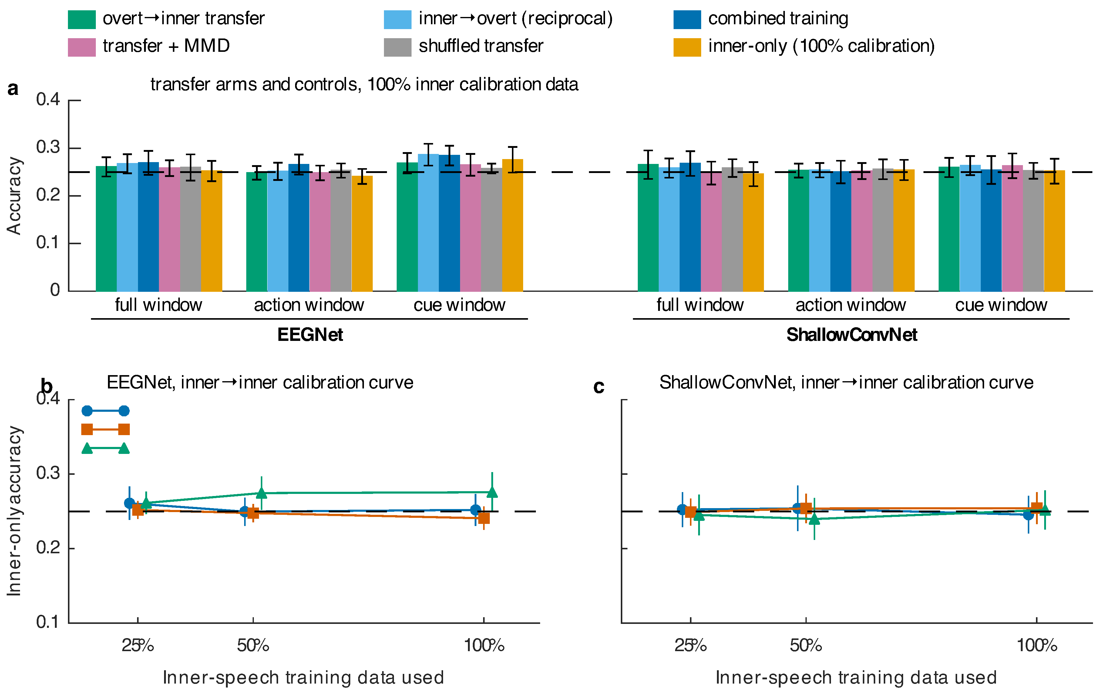
Figure 3.
Subject-dependent pooled-session (solid), held-out-session and leave-one-subject-out (hatched) accuracy in the action window for the four decoders and four arms, mean over participants with 95% CI. Grey points are individual participants, and the dashed line is chance. The numbers above the overt cluster give the pooled-session, held-out-session and LOSO means. The shuffled inner-only arm was not run under the held-out-session protocol (its shuffled overt and shuffled transfer counterparts are in Table 5). Overt speech is decodable within participant, less so when the test session is held out, and not across participants. Inner speech, transfer and the shuffled control are not distinguishable from chance under any protocol.
Figure 3.
Subject-dependent pooled-session (solid), held-out-session and leave-one-subject-out (hatched) accuracy in the action window for the four decoders and four arms, mean over participants with 95% CI. Grey points are individual participants, and the dashed line is chance. The numbers above the overt cluster give the pooled-session, held-out-session and LOSO means. The shuffled inner-only arm was not run under the held-out-session protocol (its shuffled overt and shuffled transfer counterparts are in Table 5). Overt speech is decodable within participant, less so when the test session is held out, and not across participants. Inner speech, transfer and the shuffled control are not distinguishable from chance under any protocol.
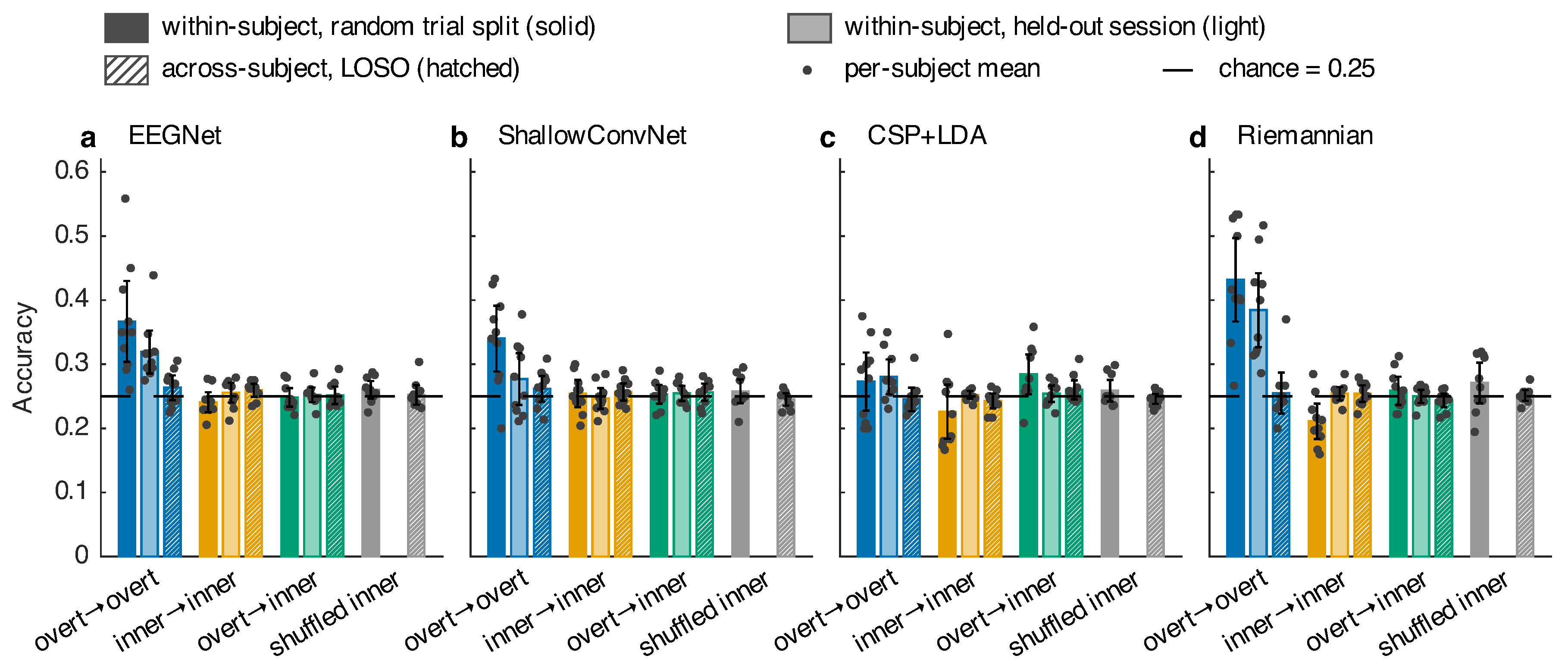
Figure 4.
Per-participant overt accuracy within participant (horizontal) against leave-one-subject-out (vertical), one marker per participant and model. Dashed lines show chance. The vertical grey band marks the within-participant binomial threshold, which applies to the horizontal axis (0.400–0.417, 20–24 test trials). The horizontal grey band marks the LOSO threshold, which applies to the vertical axis (0.317–0.324, 100–120 test trials). The legend counts participants above each threshold (within | LOSO). Of the 40 points, 34 fall below the diagonal. One point (Riemannian, participant 03) exceeds the LOSO threshold.
Figure 4.
Per-participant overt accuracy within participant (horizontal) against leave-one-subject-out (vertical), one marker per participant and model. Dashed lines show chance. The vertical grey band marks the within-participant binomial threshold, which applies to the horizontal axis (0.400–0.417, 20–24 test trials). The horizontal grey band marks the LOSO threshold, which applies to the vertical axis (0.317–0.324, 100–120 test trials). The legend counts participants above each threshold (within | LOSO). Of the 40 points, 34 fall below the diagonal. One point (Riemannian, participant 03) exceeds the LOSO threshold.
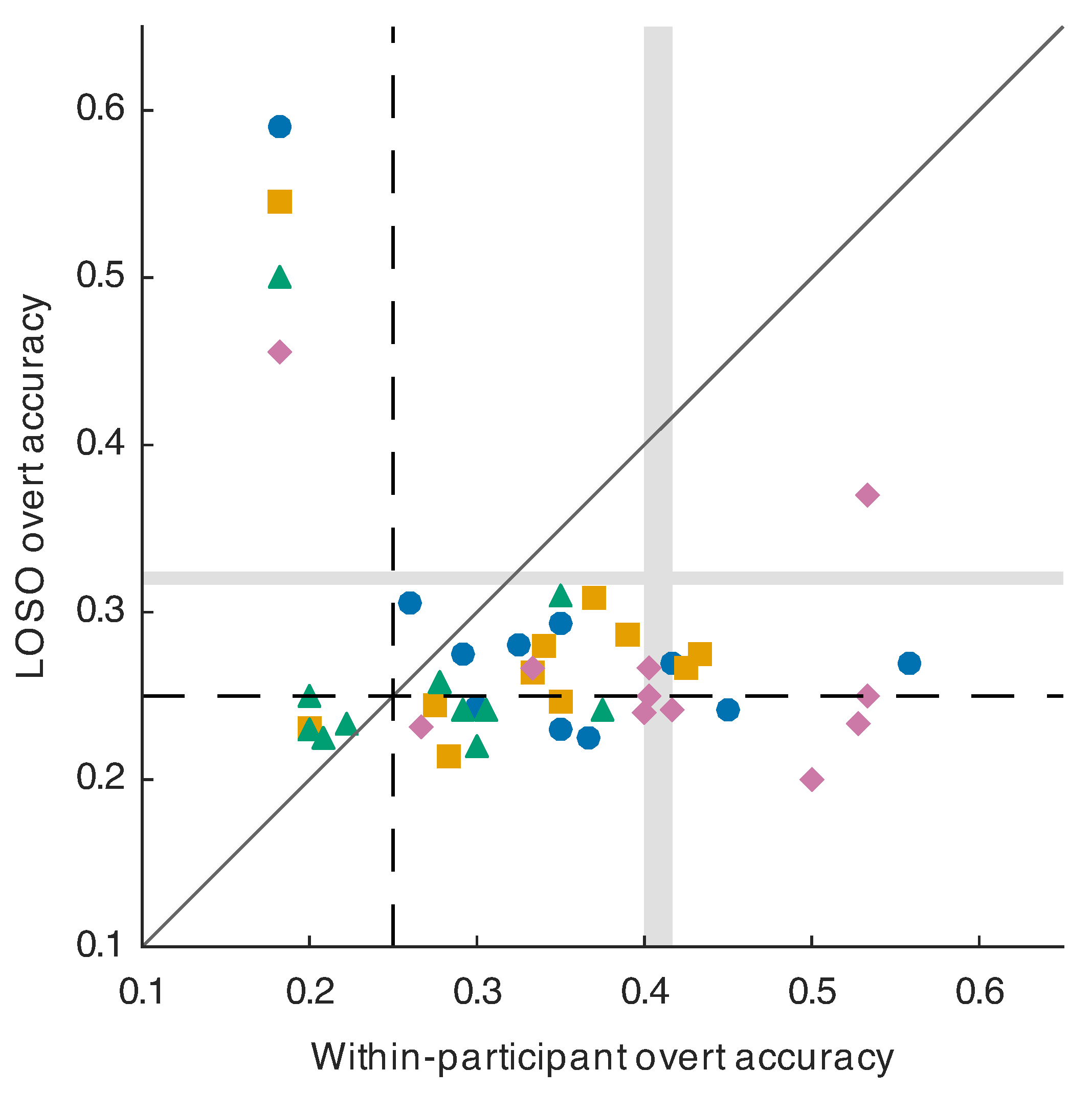
Figure 5.
(a) EEGNet overt-only and inner-only accuracy in the action window from 12 position-based channel conditions (random draws of equal size pooled), mean over participants with 95% CI. (b) Overt-only, inner-only and transfer accuracy for the four decoders on the broadband signal, after an 8–30 Hz band-pass and after a 30–100 Hz band-pass, with shuffled-label controls. The network overt signal disappears in 8–30 Hz. A reduced overt signal remains there for the covariance-based pipelines. Every decoder reads overt speech best in 30–100 Hz. Inner-only and transfer are not distinguishable from chance in any band. The all-channel EEGNet overt values in (a) (0.342, three seeds, separate run) and in (b) (0.367, five seeds) come from different runs of the same configuration. Their intervals overlap.
Figure 5.
(a) EEGNet overt-only and inner-only accuracy in the action window from 12 position-based channel conditions (random draws of equal size pooled), mean over participants with 95% CI. (b) Overt-only, inner-only and transfer accuracy for the four decoders on the broadband signal, after an 8–30 Hz band-pass and after a 30–100 Hz band-pass, with shuffled-label controls. The network overt signal disappears in 8–30 Hz. A reduced overt signal remains there for the covariance-based pipelines. Every decoder reads overt speech best in 30–100 Hz. Inner-only and transfer are not distinguishable from chance in any band. The all-channel EEGNet overt values in (a) (0.342, three seeds, separate run) and in (b) (0.367, five seeds) come from different runs of the same configuration. Their intervals overlap.
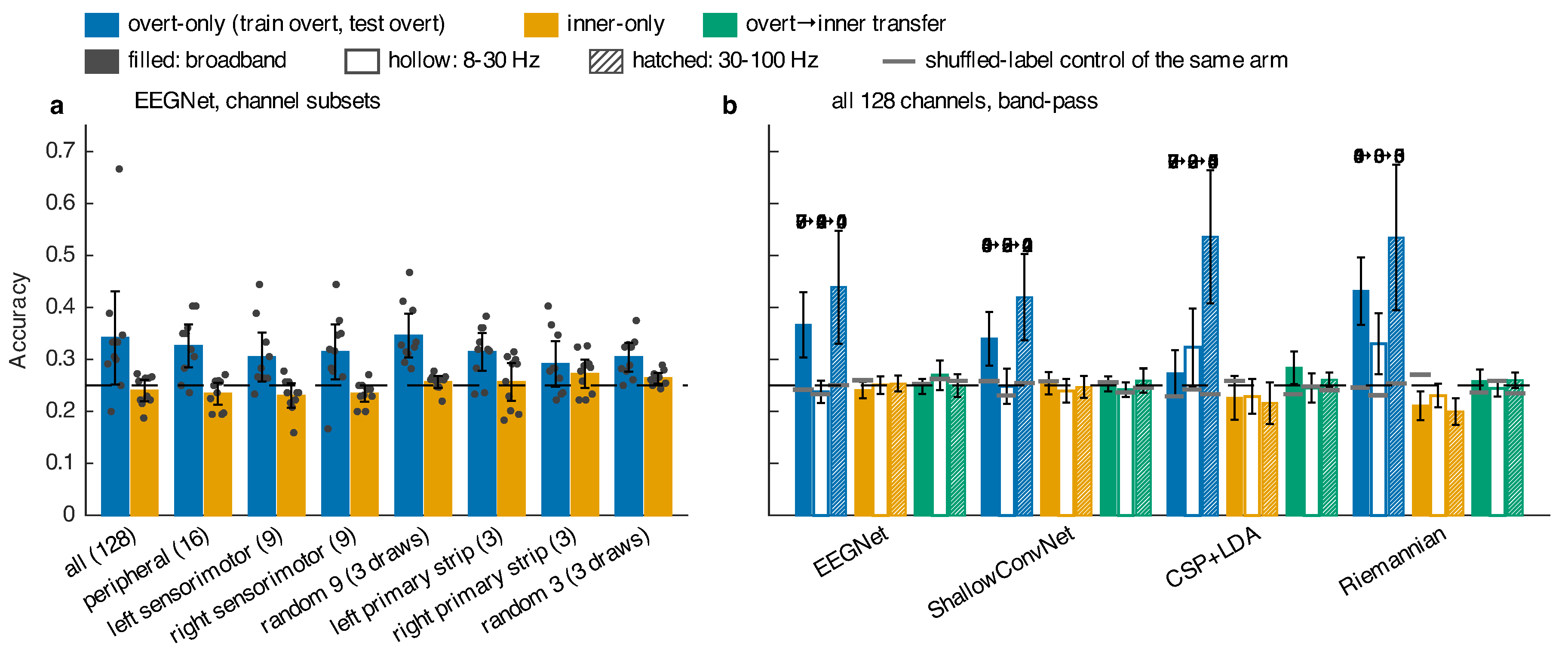
Table 1.
Trials per participant after the dataset authors’ artefact rejection, pooled over the three sessions. Classes are balanced within every cell.
Table 1.
Trials per participant after the dataset authors’ artefact rejection, pooled over the three sessions. Classes are balanced within every cell.
| Participant | 01 | 02 | 03 | 04 | 05 | 06 | 07 | 08 | 09 | 10 |
| Pronounced | 100 | 120 | 100 | 120 | 120 | 108 | 120 | 100 | 120 | 120 |
| Inner speech | 200 | 240 | 180 | 240 | 240 | 216 | 240 | 200 | 240 | 240 |
Table 2.
Network architectures as used (input samples, four outputs). Parameter counts are given for the full (), action () and cue () windows.
Table 2.
Network architectures as used (input samples, four outputs). Parameter counts are given for the full (), action () and cue () windows.
| Model | Layers | Full | Action | Cue |
|---|---|---|---|---|
| EEGNet | temporal conv (), BN; depthwise spatial conv (), BN, ELU, avg-pool , dropout 0.5; separable conv (), BN, ELU, avg-pool , dropout 0.5; flatten; linear | 4308 | 3796 | 3412 |
| ShallowConvNet | temporal conv (40 filters); spatial conv (40 filters), BN; square; avg-pool stride 15; log; dropout 0.5; flatten; linear | 217 244 | 211 804 | 207 644 |
Table 4.
Action-window arms on epochs rebuilt from the raw recordings without independent component analysis (three seeds). Values are means over ten participants [95% t-CI], followed by the number of participants above chance and above their binomial threshold. The value on the derivatives for the same seeds is in parentheses. Shuffled-label counterparts in italics. Holm correction over the 28 cells of this table.
Table 4.
Action-window arms on epochs rebuilt from the raw recordings without independent component analysis (three seeds). Values are means over ten participants [95% t-CI], followed by the number of participants above chance and above their binomial threshold. The value on the derivatives for the same seeds is in parentheses. Shuffled-label counterparts in italics. Holm correction over the 28 cells of this table.
| Arm | EEGNet | ShallowConvNet | CSP+LDA | Riemannian |
|---|---|---|---|---|
| Overt-only (pron.→pron.) | 0.492 [0.396, 0.587]; 10, 5 (0.354) | 0.560 [0.460, 0.659]; 10, 9 (0.336) | 0.386 [0.295, 0.478]; 8, 4 (0.273) | 0.600 [0.507, 0.692]; 10, 9 (0.432) |
| shuffled overt | 0.241 | 0.253 | 0.245 | 0.237 |
| Inner-only (inner→inner) | 0.249 [0.236, 0.263]; 4, 0 (0.239) | 0.245 [0.220, 0.271]; 3, 0 (0.249) | 0.260 [0.233, 0.286]; 6, 0 (0.226) | 0.218 [0.183, 0.253]; 3, 0 (0.211) |
| shuffled inner | 0.252 | 0.266 | 0.251 | 0.254 |
| Transfer (pron.→inner) | 0.252 [0.227, 0.277]; 4, 0 (0.247) | 0.259 [0.234, 0.284]; 7, 0 (0.252) | 0.275 [0.250, 0.300]; 8, 0 (0.284) | 0.258 [0.234, 0.281]; 4, 0 (0.259) |
| shuffled transfer | 0.264 | 0.255 | 0.259 | 0.249 |
| Reciprocal (inner→pron.) | 0.251 [0.229, 0.272]; 5, 0 (0.255) | 0.246 [0.225, 0.267]; 4, 0 (0.253) | 0.245 [0.233, 0.257]; 4, 0 (0.255) | 0.268 [0.239, 0.298]; 6, 1 (0.267) |
Table 5.
Held-out-session accuracy in the action window (one session tested, two trained; three seeds; 30 session–participant rows per cell). Values are means over ten participants [95% t-CI], followed by the number of participants above chance and above their binomial threshold (0.400 pronounced, 0.375 inner). Shuffled-label counterparts in italics. Holm correction over the 24 cells of this table.
Table 5.
Held-out-session accuracy in the action window (one session tested, two trained; three seeds; 30 session–participant rows per cell). Values are means over ten participants [95% t-CI], followed by the number of participants above chance and above their binomial threshold (0.400 pronounced, 0.375 inner). Shuffled-label counterparts in italics. Holm correction over the 24 cells of this table.
| Arm | EEGNet | ShallowConvNet | CSP+LDA | Riemannian |
|---|---|---|---|---|
| Overt-only | 0.319 [0.286, 0.353]; 10, 1 | 0.277 [0.236, 0.317]; 6, 0 | 0.280 [0.253, 0.307]; 8, 0 | 0.384 [0.327, 0.442]; 10, 5 |
| shuffled overt | 0.251 | 0.247 | 0.257 | 0.253 |
| Inner-only | 0.256 [0.240, 0.271]; 6, 0 | 0.247 [0.231, 0.263]; 3, 0 | 0.252 [0.246, 0.258]; 6, 0 | 0.254 [0.244, 0.264]; 6, 0 |
| Transfer | 0.252 [0.241, 0.264]; 5, 0 | 0.255 [0.243, 0.266]; 6, 0 | 0.254 [0.241, 0.267]; 6, 0 | 0.250 [0.240, 0.260]; 5, 0 |
| shuffled transfer | 0.252 | 0.251 | 0.248 | 0.245 |
| Reciprocal | 0.242 [0.222, 0.263]; 4, 0 | 0.249 [0.226, 0.272]; 3, 0 | 0.267 [0.250, 0.283]; 8, 0 | 0.257 [0.234, 0.279]; 6, 0 |
Table 6.
Paired effects in the action window, in percentage points. Each entry is the mean over ten participants of the per-participant difference [95% t-CI], followed by the approximate smallest difference detectable at one-sided with 80% power, before correction (t approximation, Equation 10). Pairs score the same held-out inner-speech trials. Transfer rows use the seeds of Table 3, and fine-tune rows the three re-run seeds of Table 7. No difference survives Holm correction within its family.
Table 6.
Paired effects in the action window, in percentage points. Each entry is the mean over ten participants of the per-participant difference [95% t-CI], followed by the approximate smallest difference detectable at one-sided with 80% power, before correction (t approximation, Equation 10). Pairs score the same held-out inner-speech trials. Transfer rows use the seeds of Table 3, and fine-tune rows the three re-run seeds of Table 7. No difference survives Holm correction within its family.
| Difference | EEGNet | ShallowConvNet | CSP+LDA | Riemannian |
|---|---|---|---|---|
| Inner-only − chance | −0.9 [−2.5, +0.6]; 1.9 | +0.4 [−1.7, +2.6]; 2.6 | −2.4 [−6.6, +1.8]; 5.1 | −3.9 [−6.6, −1.1]; 3.3 |
| Transfer − inner-only | +0.8 [−0.6, +2.1]; 1.6 | −0.1 [−2.4, +2.1]; 2.7 | +5.8 [+0.9, +10.8]; 5.9 | +4.8 [+0.7, +8.8]; 4.9 |
| Transfer − shuffled transfer | −0.5 [−2.4, +1.5]; 2.3 | −0.3 [−3.1, +2.6]; 3.5 | +5.1 [+0.8, +9.3]; 5.1 | +2.2 [−0.1, +4.6]; 2.9 |
| Fine-tune − inner-only (25%) | +1.6 [−1.9, +5.0]; 4.1 | +1.2 [−2.2, +4.6]; 4.1 | – | – |
| Fine-tune − inner-only (50%) | +3.2 [−0.1, +6.5]; 4.0 | +0.9 [−1.2, +3.1]; 2.6 | – | – |
| Fine-tune − inner-only (100%) | +0.9 [−1.9, +3.7]; 3.4 | +0.3 [−2.7, +3.4]; 3.6 | – | – |
Table 7.
Fine-tuning arms in the action window (three seeds). Values are means over ten participants [95% t-CI] on the same held-out inner-speech trials as Table 3, chance 0.250. Target-only trains from scratch on the inner-speech subset. It was re-run alongside the other two arms so that the comparison is paired. Fine-tune pre-trains on pronounced speech first. Shuffled pre-training permutes the pronounced labels before pre-training. No participant exceeded the binomial threshold (0.375) in any cell. Holm correction over the 18 cells of this table gives everywhere.
Table 7.
Fine-tuning arms in the action window (three seeds). Values are means over ten participants [95% t-CI] on the same held-out inner-speech trials as Table 3, chance 0.250. Target-only trains from scratch on the inner-speech subset. It was re-run alongside the other two arms so that the comparison is paired. Fine-tune pre-trains on pronounced speech first. Shuffled pre-training permutes the pronounced labels before pre-training. No participant exceeded the binomial threshold (0.375) in any cell. Holm correction over the 18 cells of this table gives everywhere.
| EEGNet | ShallowConvNet | |||||
|---|---|---|---|---|---|---|
| Inner training set | Target-only | Fine-tune | Shuffled pre-tr. | Target-only | Fine-tune | Shuffled pre-tr. |
| 25% | 0.245 [0.225, 0.265] | 0.261 [0.231, 0.290] | 0.240 [0.215, 0.266] | 0.247 [0.215, 0.279] | 0.259 [0.240, 0.278] | 0.250 [0.227, 0.274] |
| 50% | 0.236 [0.212, 0.259] | 0.268 [0.240, 0.295] | 0.241 [0.207, 0.275] | 0.258 [0.236, 0.279] | 0.267 [0.251, 0.283] | 0.248 [0.225, 0.271] |
| 100% | 0.239 [0.219, 0.260] | 0.249 [0.218, 0.279] | 0.242 [0.209, 0.275] | 0.253 [0.223, 0.283] | 0.256 [0.221, 0.292] | 0.257 [0.239, 0.275] |
Table 8.
Leave-one-subject-out accuracy in the action window. Values are means over ten held-out participants [95% t-CI], followed by the number of participants above chance. Holm-corrected in every cell. One participant exceeded its binomial threshold in Riemannian overt-LOSO and one in CSP+LDA transfer-LOSO. None did in any other cell.
Table 8.
Leave-one-subject-out accuracy in the action window. Values are means over ten held-out participants [95% t-CI], followed by the number of participants above chance. Holm-corrected in every cell. One participant exceeded its binomial threshold in Riemannian overt-LOSO and one in CSP+LDA transfer-LOSO. None did in any other cell.
| Arm | EEGNet | ShallowConvNet | CSP+LDA | Riemannian |
|---|---|---|---|---|
| Overt-LOSO | 0.263 [0.244, 0.283]; 6 | 0.262 [0.241, 0.282]; 6 | 0.245 [0.227, 0.263]; 2 | 0.255 [0.223, 0.287]; 3 |
| Inner-LOSO | 0.259 [0.249, 0.270]; 8 | 0.257 [0.243, 0.270]; 6 | 0.243 [0.231, 0.254]; 2 | 0.254 [0.241, 0.267]; 5 |
| Transfer-LOSO | 0.252 [0.238, 0.265]; 3 | 0.256 [0.243, 0.270]; 7 | 0.260 [0.245, 0.275]; 5 | 0.244 [0.233, 0.254]; 2 |
| Shuffled inner-LOSO | 0.252 | 0.245 | 0.246 | 0.251 |
Table 11.
Action-window arms on the external electrodes and on the regressed scalp (three seeds). Values are means over ten participants [95% t-CI], followed by the number of participants above chance and above their binomial threshold (0.400–0.417 for the overt test sets, 0.354–0.375 for the inner test sets). Seeds 0–2 of the splits of Table 3 were used, so the regressed-scalp arms score the same test trials as the broadband arms of those seeds. The broadband row restates those three seeds (the network values in Table 3 average five), and the paired drops in the text are computed against it. Shuffled overt controls in italics. The shuffled inner and transfer controls were 0.235–0.269 and are omitted. Holm correction over the 72 cells of this run has a floor of 0.070 and is descriptive. The uncorrected one-sided p is 0.001 for every overt cell on the external electrodes and for the Riemannian regressed-scalp cell.
Table 11.
Action-window arms on the external electrodes and on the regressed scalp (three seeds). Values are means over ten participants [95% t-CI], followed by the number of participants above chance and above their binomial threshold (0.400–0.417 for the overt test sets, 0.354–0.375 for the inner test sets). Seeds 0–2 of the splits of Table 3 were used, so the regressed-scalp arms score the same test trials as the broadband arms of those seeds. The broadband row restates those three seeds (the network values in Table 3 average five), and the paired drops in the text are computed against it. Shuffled overt controls in italics. The shuffled inner and transfer controls were 0.235–0.269 and are omitted. Holm correction over the 72 cells of this run has a floor of 0.070 and is descriptive. The uncorrected one-sided p is 0.001 for every overt cell on the external electrodes and for the Riemannian regressed-scalp cell.
| Signal and arm | EEGNet | ShallowConvNet | CSP+LDA | Riemannian |
|---|---|---|---|---|
| Eight external electrodes (EXG1–8) | ||||
| Overt-only | 0.659 [0.538, 0.781]; 10, 9 | 0.813 [0.691, 0.935]; 10, 10 | 0.794 [0.693, 0.896]; 10, 10 | 0.902 [0.829, 0.975]; 10, 10 |
| shuffled overt | 0.224 | 0.256 | 0.256 | 0.243 |
| Inner-only | 0.255 [0.236, 0.273]; 4, 0 | 0.262 [0.234, 0.290]; 5, 0 | 0.259 [0.237, 0.281]; 6, 0 | 0.258 [0.226, 0.290]; 6, 0 |
| Transfer | 0.250 [0.228, 0.273]; 4, 0 | 0.258 [0.219, 0.296]; 3, 1 | 0.251 [0.247, 0.256]; 4, 0 | 0.251 [0.244, 0.258]; 1, 0 |
| Lip pair (EXG7–8) | ||||
| Overt-only | 0.686 [0.582, 0.791]; 10, 10 | 0.826 [0.729, 0.923]; 10, 10 | 0.668 [0.596, 0.739]; 10, 10 | 0.707 [0.612, 0.803]; 10, 10 |
| shuffled overt | 0.256 | 0.255 | 0.276 | 0.255 |
| Inner-only | 0.260 [0.239, 0.281]; 7, 0 | 0.262 [0.230, 0.294]; 6, 0 | 0.249 [0.218, 0.280]; 3, 0 | 0.236 [0.205, 0.267]; 4, 0 |
| Transfer | 0.237 [0.215, 0.260]; 3, 0 | 0.251 [0.242, 0.259]; 2, 0 | 0.249 [0.234, 0.265]; 1, 0 | 0.248 [0.233, 0.264]; 2, 0 |
| 128 scalp channels, EXG regressed out (Equation 1) | ||||
| Overt-only | 0.304 [0.272, 0.336]; 9, 0 | 0.279 [0.243, 0.315]; 7, 0 | 0.306 [0.239, 0.374]; 7, 2 | 0.402 [0.335, 0.468]; 10, 4 |
| shuffled overt | 0.242 | 0.236 | 0.244 | 0.230 |
| broadband scalp, seeds 0–2 | 0.354 | 0.336 | 0.273 | 0.432 |
| Inner-only | 0.232 [0.211, 0.254]; 3, 0 | 0.260 [0.235, 0.284]; 6, 0 | 0.220 [0.194, 0.246]; 1, 0 | 0.212 [0.184, 0.240]; 2, 0 |
| Transfer | 0.253 [0.234, 0.271]; 4, 0 | 0.271 [0.245, 0.297]; 6, 0 | 0.261 [0.235, 0.286]; 6, 0 | 0.244 [0.217, 0.270]; 4, 0 |
Disclaimer/Publisher’s Note: The statements, opinions and data contained in all publications are solely those of the individual author(s) and contributor(s) and not of MDPI and/or the editor(s). MDPI and/or the editor(s) disclaim responsibility for any injury to people or property resulting from any ideas, methods, instructions or products referred to in the content. |
© 2026 by the authors. Licensee MDPI, Basel, Switzerland. This article is an open access article distributed under the terms and conditions of the Creative Commons Attribution (CC BY) license (http://creativecommons.org/licenses/by/4.0/).
Copyright: This open access article is published under a Creative Commons CC BY 4.0 license, which permit the free download, distribution, and reuse, provided that the author and preprint are cited in any reuse.