

Submitted:
11 November 2026
Posted:
12 November 2026
You are already at the latest version
Abstract
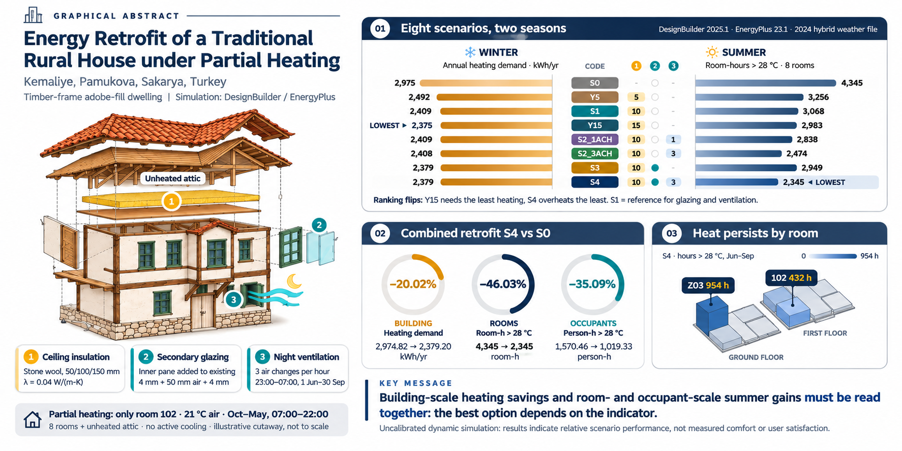
Energy retrofits of traditional dwellings require assessments that account for partial heating and differences in room use. This study evaluates ceiling insulation, secondary glazing, and controlled night ventilation in a traditional timber-frame dwelling in Kemaliye, Sakarya, Türkiye. Eight scenarios were simulated in DesignBuilder using EnergyPlus and a hybrid weather file derived from 2024 meteorological observations. Active heating was restricted to room 102. Annual heating demand and final energy consumption were assessed alongside hourly operative temperatures, summer threshold exceedances, and occupancy-weighted exposure across eight rooms. Ceiling insulation reduced heating demand, with diminishing additional savings as thickness increased. Relative to the baseline, the combined intervention reduced annual heating demand by 20.02%, final energy consumption by 13.68%, and summer exceedance above 28 °C by 46.03%. Night ventilation improved summer performance without appreciably changing heating demand, whereas secondary glazing provided limited additional energy savings. Occupancy-weighted nighttime exposure increased after insulation despite a decrease in total nighttime exceedance. Winter operative temperatures remained low despite attainment of the air temperature setpoint. These findings support evaluating retrofit options through energy indicators and thermal conditions in occupied rooms. Results are specific to the modeled dwelling, occupancy assumptions, and weather data; the model was not calibrated against field measurements.
Keywords:
traditional rural dwelling
; partial heating
; energy retrofitting
; building energy simulation
; thermal performance
1. Introduction
Material selection, construction systems, and spatial organization in traditional dwellings reflect local environmental knowledge and everyday practices. Battistella [1] examines the relationship between traditional ecological knowledge and architectural design in the context of this accumulated environmental knowledge. Research on abandoned rural settlements in Türkiye shows that depopulation and changes in use affect the continuity of built heritage [2]. Conservation therefore encompasses sustaining the use of buildings as well as preserving their physical characteristics.
Energy retrofits can help adapt traditional dwellings to contemporary living requirements. In evaluating interventions, original building components, indoor thermal conditions, and patterns of use are important alongside energy consumption. Occupants’ thermal perceptions and their relationships with spaces can influence both energy use and conservation decisions [3]. The environmentally responsive features of a traditional building do not inherently ensure adequate thermal performance under current patterns of use. Limiting heat losses in winter and removing accumulated heat in summer may entail different requirements. Examining insulation, window, and ventilation options together allows these seasonal interactions to be assessed within the specific context of the building and its climate [4].
Partial heating is an aspect of dwelling use that directly affects this assessment. In her study of Osmaneli, Ergöz Karahan [5] notes that daily life during winter may be concentrated in one or two rooms in stove-heated dwellings. Under such conditions, a low annual heating demand does not indicate that adequate thermal conditions are achieved throughout the dwelling. The room-level and seasonal assessment conducted by Basaly et al. [6] also illustrates the examination of energy results alongside thermal conditions in individual rooms. These studies highlight the importance of patterns of use and spatial differences in assessments of energy and thermal performance. However, the central focus of this study is to compare both the building-level benefits of energy retrofit interventions in traditional dwellings and their room-level outcomes in relation to occupancy schedules.
Within this framework, the central research question is the extent to which the building-level benefits of energy retrofit interventions in a partially heated traditional dwelling are reflected in thermal conditions in occupied rooms during periods of use. The study compares ceiling insulation, secondary glazing, and controlled night ventilation across eight scenarios for a partially heated traditional dwelling in Kemaliye. The effects of these interventions on annual heating demand and summer temperature exceedances are examined at both building and room levels, considering daytime and nighttime periods and the defined occupancy schedule. The study also investigates how occupancy-weighted temperature exceedance indicators alter the performance ranking of the scenarios. Its main contribution lies in revealing, within a single comparative assessment framework, the divergence between building-level benefits and thermal conditions in occupied rooms during periods of use. In doing so, the study aims to support the evaluation of energy retrofit decisions for traditional dwellings in conjunction with patterns of use and architectural conservation requirements.
2. Literature Review
Research on the energy and thermal performance of traditional dwellings focuses on key variables affecting thermal performance, including the relationships among local climatic conditions, the physical properties of building materials, occupant behavior, and natural ventilation strategies. Improving the energy performance of these buildings is a multidimensional research challenge that also involves preserving their character and authenticity. Particularly in historic buildings, factors such as indoor temperatures and patterns of use should be assessed together, with careful consideration of the compatibility of proposed interventions with the existing building.
Lozoya-Peral et al. [4] investigated a traditional dwelling in the Mediterranean climate of southeastern Spain using DesignBuilder to analyze the effects of building envelope insulation, natural ventilation strategies, window dimensions, and glazing properties on energy demand and indoor temperatures. The study showed that improving the insulation of the building envelope could reduce heating demand but could also prolong periods of elevated indoor temperatures. Natural ventilation was found to help limit indoor overheating during the summer months. These findings indicate that the assessment of energy retrofit strategies should consider thermal conditions across different seasons alongside annual energy consumption [4].
Improving the energy performance of traditional buildings constitutes an important research area within the literature on architectural heritage conservation, which seeks to meet occupant needs while preserving the original attributes of buildings. Karabeyeser Bakan et al. [3] examined the role of thermal comfort expectations in energy efficiency approaches and architectural conservation decisions through interviews with occupants of three historic dwellings in the Bey neighborhood of Gaziantep. Their study showed that the values occupants attach to historic buildings and their thermal comfort expectations influence energy retrofit decisions. Fiore et al. [7] conducted a systematic review of 69 studies, assessing the compatibility between architectural conservation and energy efficiency in historic buildings in terms of aesthetic, technical, and energy performance criteria. The researchers emphasized that interventions should be evaluated in terms of their effects on historic features, their reversibility, and their compatibility with existing building materials. These studies highlight the need to assess decisions concerning energy performance improvements in traditional dwellings in conjunction with their architectural characteristics and material composition.
Studies assessing indoor environmental performance in traditional dwellings show that the physical characteristics of buildings and patterns of space use are interrelated and should be examined together. In a systematic review of 105 studies on factors influencing occupant satisfaction in vernacular architecture, Shetty and Patil [8] assessed the relationships between occupant satisfaction and the use of local materials, natural ventilation, spatial organization, and sociocultural factors. Their findings indicate that satisfaction with the indoor environment in traditional dwellings cannot be explained solely by building envelope components; spatial practices and occupant expectations should also be examined within a holistic assessment framework.
The interaction between thermal comfort and occupant behavior is examined from a broader perspective in the adaptive thermal comfort literature. Brager and de Dear [9] explained occupants’ adaptation to the thermal environment in terms of physiological, behavioral, and psychological factors, noting that comfort perceptions in naturally ventilated buildings may differ from those in mechanically conditioned buildings. In their work on adaptive thermal comfort, de Dear et al. [10] emphasized climatic conditions, building typology, and occupant expectations as critical factors shaping thermal comfort. These studies show that indoor temperature alone does not reflect occupants’ perceptions of comfort and that thermal conditions should be considered within the context of building use. This approach is particularly relevant to traditional rural dwellings. Under patterns of use in which spaces are not heated simultaneously and heating is restricted to specific rooms and limited hours, building-level energy demand alone is insufficient to characterize thermal conditions in individual rooms. Achieving the target air temperature in heated rooms does not, in itself, demonstrate that an adequate operative temperature or occupant comfort has been attained; temperatures in unheated rooms may vary depending on outdoor conditions and heat exchange between rooms. Similarly, ventilation dynamics, solar gains, floor level, and building envelope characteristics lead to spatial variations in indoor temperatures during summer. Assessing aggregate building-level energy indicators alongside room-level temperature data is therefore particularly important when evaluating the energy performance of traditional dwellings.
The seasonal outcomes of building envelope retrofit strategies call for a dedicated assessment framework to examine the interaction between summer overheating and energy performance. While thermal insulation reduces heat losses in winter, its effects on indoor temperatures in summer vary depending on ventilation conditions, solar gains, and internal heat loads. The findings of Lozoya-Peral et al. [4] highlight the importance of a comparative approach centered on seasonal variations for accurately interpreting the effects of ventilation, insulation, and glazing interventions in traditional dwellings. Accordingly, high indoor temperatures in summer and heating demand in winter should be assessed together when evaluating energy retrofit scenarios.
The accurate interpretation of research findings depends on the indicators used to quantify summer overheating. Although the total duration above a specified temperature threshold provides information about overheating, it does not, by itself, capture the magnitude of the exceedance. A degree-hour indicator combines the duration and magnitude of temperature exceedances, enabling a more comprehensive assessment. Assigning equal weight to temperature exceedances across rooms at the building level may obscure differences in how these spaces are used. Relating exceedance durations to occupancy schedules therefore allows scenarios to be compared in terms of potential occupant exposure. However, these indicators should not be interpreted as measurements of actual occupants’ satisfaction with thermal comfort or their thermal experiences.
Taken together, existing studies show that the effects of energy retrofit strategies in traditional dwellings on indoor comfort conditions, energy consumption, and the preservation of historic fabric have been investigated using various methodologies. However, particularly under partial heating conditions, the joint assessment of building-level energy savings, room-level temperature exceedances, and exposure indicators accounting for occupancy duration within a single comparative framework warrants further investigation. This research need stems not from a lack of previous studies on interventions such as natural ventilation, insulation, and window improvements, but from the additional insights that can be gained by interpreting their effects through multiple performance indicators. Table 1 compares the scope of selected studies with that of the present research.
The studies compared in Table 1 highlight the importance of evaluating energy retrofit interventions in traditional dwellings in conjunction with building envelope characteristics, climatic conditions, natural ventilation, occupant needs, and architectural conservation principles. While Timur et al. [11], Dervishi et al. [12], and Lozoya-Peral et al. [4] examined the performance effects of energy retrofit interventions under different building and climatic conditions, Karabeyeser Bakan et al. [3] and Shetty and Patil [8] focused on the relationship between occupant experience and indoor environmental conditions. These studies support the methodological framework of the Kemaliye study while highlighting the need for research that jointly compares building-level energy savings and room-level temperature exceedances in relation to occupancy hours under partial heating conditions. Accordingly, the distinctive approach of this study lies in comparing the same energy retrofit scenarios in terms of annual heating demand, room-level operative temperatures, durations of temperature threshold exceedance, degree-hour values, and exposure indicators linked to the occupancy schedule. The effects of different interventions on energy performance and summer overheating are thus assessed while accounting for differences between aggregate building-level results and thermal conditions in occupied rooms. Rather than proposing a single retrofit solution that can be generalized to traditional rural dwellings, the study examines the role of different performance indicators in selecting interventions under specific building and occupancy conditions.
3. Materials and Methods
This research is a comparative numerical case study of a single traditional dwelling. Eight scenarios, encompassing the existing condition and interventions involving ceiling insulation, secondary glazing, and controlled night ventilation, were simulated over a full year using the same Kemaliye–Pamukova hybrid EnergyPlus Weather (EPW) file. Building geometry, room floor areas and volumes, and inputs outside the scope of the interventions were held constant. The analysis is based on the relative changes in energy and thermal performance resulting from the interventions compared with the existing condition or the relevant reference scenario.
3.1. Study Area and Architectural Characteristics of the Case Study Building
The study was conducted in a traditional dwelling in Kemaliye, a settlement in Pamukova district, Sakarya province. Along with Çilekli and Hüseyinli, Kemaliye is one of the settlements included in a regional study on tourism routes focused on rural development [13]. According to official information provided by a local authority, the settlement is approximately 22 km from Pamukova district center and 67 km from Sakarya provincial center [14]. The location of the dwelling within the settlement and its immediate surroundings are shown in Figure 1.
The dwelling is located in the southern part of Kemaliye’s built-up area, on cadastral block 209, parcel 17, at approximately 40.522593° N and 30.004136° E. Its timber frame with adobe infill rests on stone foundation walls, and the wall surfaces are finished with lime-based plaster (Figure 2).
The staircase and door and window joinery are made of timber, and the roof is covered with curved clay tiles. The combined use of stone, timber, adobe, and lime-based plaster reflects the material and construction characteristics of Kemaliye’s traditional residential fabric. For energy modeling purposes, the dwelling was assessed on the assumption that its existing building components remained intact and that no significant physical damage was present. This assumption does not imply that the building’s structural safety or material strength has been verified through detailed technical investigations.
The two-story dwelling is entered through the ground-floor hall (sofa), designated Z01, which provides access to the other ground-floor spaces. A timber staircase connects this space to the first-floor hall, designated 101. Rooms Z02, Z03, and Z04 are currently used to store equipment for agriculture and livestock farming; the adjoining roofed, open-sided outbuilding serves the same function. This pattern of use illustrates the functional links of the dwelling and its outbuilding to rural production activities.
Rooms 102, 103, and 104 on the first floor are accessed from hall 101. Rooms 102 and 104 retain the traditional room layout, each with a hearth flanked by built-in storage cupboards. Storing mattresses and quilts in these cupboards allows the rooms to accommodate sitting, sleeping, and dining activities (Figure 3).
3.2. Development of the Building Energy Model
A building energy model was developed in DesignBuilder 2025.1.1.011 to assess the thermal performance of the traditional dwelling in its existing condition and compare the effects of retrofit scenarios. The model was based on the building’s architectural geometry, construction system, material properties, and spatial organization, together with the number of occupants, room occupancy schedules, and heating conditions. To ensure comparability across scenarios, building geometry and room floor areas and volumes were held constant, and only the model parameters representing the relevant intervention were modified in each scenario. The effects of the retrofits on energy consumption and indoor thermal conditions were thus evaluated under common modeling assumptions.
3.2.1. Model Geometry and Thermal Zoning
The building energy model included eight rooms, coded Z01–Z04 on the ground floor and 101–104 on the first floor (Figure 4). The attic was modeled as a separate thermal zone, with no active heating system assigned to it.
The geometry of the heat transfer surfaces was defined using the building’s external dimensions, whereas room floor areas and volumes were calculated using the internal dimensions option (Table 2). Using different dimensional bases for surface geometry and room area and volume calculations may result in differences between the projected areas of floor surfaces and the room floor areas defined in the model [21]. This approach to area and volume calculations was maintained across all scenarios.
The eight rooms defined in the model have a total floor area of 105.726 m² and a total volume of 278.5404 m³. The unheated attic, with a floor area of 78.4625 m² and a volume of 62.7098 m³, was assessed separately and excluded from these totals.
Floor elevations were set at 0.00, 2.70, and 5.40 m, and net room air volumes were calculated taking surface thicknesses into account.
The model included 151 heat transfer surfaces and 11 external windows. Paired surface records representing opposite sides of internal building elements were not counted twice when determining the number of physical elements. The total area of the window glazing planes defined in the IDF (Input Data File), which contains the EnergyPlus simulation inputs, is approximately 5.147 m². This value represents the glazing planes and differs from the gross architectural opening area, which also includes the frames. Nearby trees and adjoining and neighboring building elements were represented using shading geometries and held constant across all scenarios.
3.2.2. Building Envelope and Material Representation
In the building energy model, the materials constituting the building elements were defined by their thermal conductivity (λ, W/(m·K)), density (ρ, kg/m³), and specific heat capacity (cₚ, J/(kg·K)). These parameters are among the fundamental material inputs used in DesignBuilder to calculate the thermal behavior of construction layers [22].
The thermophysical properties and record names of the materials used in the model are presented in Table 3. The numerical values are based on the Material objects in the EnergyPlus input data files (IDFs) used in this study.
Wall sections comprising timber framing and adobe infill were represented in the model by a single layer with equivalent thermophysical properties. External walls were defined with a total thickness of 20 cm, consisting, from outside to inside, of 2 cm of lime plaster, a 16 cm equivalent timber frame–adobe infill layer, and 2 cm of lime plaster. Internal partitions were assumed to have an equivalent core layer thickness of 12 cm and a total wall thickness of 16 cm. The thermal behavior of the walls was calculated using the equivalent layer properties; detailed heat transfer at the interfaces between the timber frame and adobe infill was not explicitly modeled. The dwelling’s floor system consists of structural timber members and timber boarding layers. In the baseline model, the timber boarding of the ceiling separating the upper-floor rooms from the unheated attic was assigned a thickness of 2 cm, while the timber boarding of the ground floor, intermediate floor, and floors exposed to outdoor air was assigned a thickness of 3 cm. The thermal representation of the ceilings and floors was based on these boarding layers. The roof covering was defined, from outside to inside, as a 2 cm clay tile layer and a 2.5 cm timber boarding layer, while the stone foundation wall was modeled with a thickness of 50 cm. The material properties and layer assumptions for the building elements are presented in Table 3 and Table 4.
A three-dimensional energy model of the dwelling was developed in DesignBuilder based on the building components and layer thicknesses presented in Table 4. The model represented the building geometry, roof form, and arrangement of openings. Nearby trees and neighboring building masses were also included to account for shading from the surrounding environment. A three-dimensional view of the modeled dwelling and its immediate surroundings is presented in Figure 5.
The three-dimensional model, developed from the building geometry and the material definitions assigned to the building envelope, provides the basis for the energy and thermal performance analyses. As both building characteristics and outdoor climatic conditions are critical to interpreting the simulation results, the meteorological data used in the study and the regional climatic characteristics they represent are described in the following section.
3.3. Regional Climatic Context and Weather Data Used
According to the topographic survey map obtained from Pamukova Municipality, the dwelling is located at an elevation of 755 m [23] (Figure S1). However, the data obtained from the meteorological service specified an elevation of 700 m, which was therefore adopted for calculating atmospheric pressure in the EPW file. The monthly regression coefficients used to fill gaps in the temperature and relative humidity data are presented in Table S1 of the Supplementary Materials.
3.3.1. Regional Climate Classification for Sakarya
In the Köppen climate classification based on temperature and precipitation data for 1991–2020 from the Turkish State Meteorological Service (MGM), the Sakarya meteorological station is classified as Cfa [24]. In this classification, C denotes the warm temperate climate group, f indicates the absence of a distinct dry season, and a represents hot summer conditions, with a mean temperature of at least 22 °C in the warmest month. The Cfa classification describes the long-term temperature and precipitation regime; it does not imply that precipitation is evenly distributed throughout the year [24].
Monthly temperature and precipitation values from the 1991–2020 climate normals published by MGM for Sakarya are shown in Figure 6, while summary indicators calculated from these data are presented in Table 5 [25].
The arithmetic mean of the monthly mean temperatures was calculated as approximately 15.17 °C, while the sum of the mean monthly precipitation totals was 878.6 mm/year. The lowest monthly mean temperature is 6.4 °C in January, and the highest is 24.4 °C in August. These temperature values and the monthly distribution of precipitation are consistent with the Cfa classification reported for the Sakarya station [24,25].
Variations in temperature and precipitation throughout the year provide a basis for assessing Sakarya’s seasonal climatic characteristics. Figure 6 presents the monthly temperature and precipitation normals alongside the province’s location on the Köppen climate classification map of Türkiye, providing a visual overview of the regional climatic conditions.
Climatic conditions across Sakarya province vary spatially due to maritime and continental influences, elevation, slope aspect, and landforms. An assessment presented on Sakarya University’s Şehir Hafızası (City Memory) platform indicates that maritime influences are more pronounced on the northern slopes of the Samanlı Mountains, whereas continentality increases on the southern slopes, and precipitation patterns vary according to topographic conditions [26].
This study addressed both the reduction of winter heat losses and the limitation of summer overheating. Sakarya’s long-term climate normals were used to establish the regional climatic context, while the energy and thermal performance of the dwelling and the retrofit scenarios were evaluated using the hourly EPW file developed for Kemaliye–Pamukova.
3.3.2. Preparation of the Local Weather File
The hybrid EPW file was prepared using 2024 observational data obtained from MGM through official correspondence [27]. Kemaliye station 18915 served as the primary source for temperature and relative humidity data. Pamukova station 19118 was used to fill missing records and provide data on wind, daily total horizontal solar radiation, and sunshine duration.
UTC timestamps were converted to local time (UTC+3), and the data were organized on an end-of-hour basis. 29 February was removed to produce a 365-day series comprising 8760 hourly records. Within each seasonal period, the same daily occupancy schedule was applied to all day types.
Missing temperature and relative humidity records at the Kemaliye station were filled using monthly regression models incorporating concurrent observations from Pamukova and sine and cosine terms representing the diurnal cycle. Records from the 5th, 12th, 19th, and 26th days of each month were reserved as test data. Following evaluation on the test data, the final models used for gap filling were refitted using all available concurrent records.
Short gaps with no data available from either station were filled by linear interpolation; the longest consecutive gap encountered was two hours.
ym,h = b0,m + b1,m xP,h + b2,m sin(2πhUTC/24) + b3,m cos(2πhUTC/24)
In Equation (1), ym,h denotes the estimated temperature or relative humidity for Kemaliye, xP,h represents the concurrent observation at the Pamukova station, m denotes the month, and hUTC indicates the hour of the day in UTC. The coefficients b0,m–b3,m were estimated separately for temperature and relative humidity for each month.
Hourly records from the Pamukova station were used for wind direction and speed; eight hours of missing data were filled using vector interpolation. The data sources and extent of gap filling for the temperature, relative humidity, and wind series are presented in Table 6.
The regression models were evaluated using 993 test records. For temperature, the mean absolute error (MAE) was 1.415 °C and the bias was −0.027 °C; for relative humidity, the corresponding values were 5.413 and +0.622 percentage points, respectively. The root mean square error (RMSE) values are reported in Table 6. These metrics characterize the test performance of the interstation gap-filling models.
Daily total solar radiation incident on a horizontal plane was converted from cal/cm² to Wh/m² and distributed into hourly values using the approach of Collares-Pereira and Rabl [28]. The distribution coefficients were normalized to preserve the daily total solar radiation energy. Solar position was calculated using the NOAA equations [29], while the approach of Erbs et al. [30] was used to separate the direct and diffuse radiation components. Daily radiation totals for 364 days in the annual series were obtained from observations, and the missing value for 31 December was filled using the mean of the preceding three days.
Shortwave irradiance was set to zero during calculation intervals when the sun was below the horizon. To limit numerical amplification at low solar elevations, a lower bound of 0.065 was applied to the cosine of the solar zenith angle when calculating the clearness index, which was constrained to the range 0–1. For intervals with a solar zenith angle cosine below 0.065, direct normal irradiance was set to zero; for the remaining intervals, it was capped at the lower of 1200 W/m² and the extraterrestrial normal irradiance. Diffuse horizontal irradiance was recalculated as the difference between global horizontal irradiance and the direct horizontal component. These procedures were applied at 10-minute calculation intervals, and the results were converted to hourly radiation energy totals.
Longwave sky irradiance was estimated using the clear-sky emissivity correlation of Clark and Allen [31] and Walton’s (1983) cloud cover correction, as described in the EnergyPlus 23.1 documentation [31,32,33]. For the cloud cover input, the indicator C = 10(1 − n/N) was derived from the ratio of daily sunshine duration (n) to astronomical day length (N) and constrained to the range 0–10. The same daily indicator was used in both daytime and nighttime calculations for the corresponding day. This conversion was an approximation adopted in this study and did not represent measured hourly cloud cover data. The corrected sky emissivity was constrained to the range 0–1, and longwave irradiance was calculated using absolute air temperature and the Stefan–Boltzmann law.
Atmospheric pressure was represented by a constant value of approximately 93.19 kPa, calculated using the standard atmosphere equation for the assumed elevation of 700 m adopted during weather file preparation. Missing-data codes specified in the EPW data dictionary were used for unavailable precipitation, snow, and illuminance fields [34].
Gap filling accounted for 42.22% and 45.16% of the temperature records in June and July, respectively. The EPW file used in this study had an annual mean outdoor air temperature of 11.465 °C, with hourly minimum and maximum temperatures of −9.4 and 34.6 °C, respectively. The mean relative humidity was 75.82%, the mean wind speed was 2.219 m/s, and the annual total global horizontal irradiation was 1639.065 kWh/m². Monthly temperature ranges and irradiation totals are shown in Figure 7.
The hybrid EPW file, weather-file generation script, hourly data provenance records, and supporting methodological and quality-control documentation are provided in Supplementary File S1.
3.4. Numerical Simulation and Performance Assessment
The numerical assessment considered the effects of the interventions on both annual energy performance and room-level thermal conditions. The simulation settings, boundary conditions, retrofit scenarios, and methods used to calculate the performance indicators are described below.
3.4.1. Thermal Simulation and Boundary Conditions
Annual simulations were performed using EnergyPlus 23.1.0. Six timesteps per hour were used for zone heat balance calculations, and hourly outputs were used for the assessment. The simulation settings held constant across all scenarios are presented in Table 7.
Heat exchange with the ground was represented using Foundation:Kiva objects for the four ground-floor rooms [35]. Thermal conductivity, density, and specific heat capacity were set to 1.73 W/(m·K), 1842 kg/m³, and 419 J/(kg·K), respectively. These are the default values in Foundation:Kiva:Settings. No separate ventilated thermal zone was defined beneath the floor.
The timber mass in the ground-floor rooms was supplemented using internal thermal mass objects with an 8 cm timber layer and a total exposed surface area of 50.32 m². These objects, which do not form boundaries with the outdoor environment, represent heat storage and exchange within the rooms using an equivalent thermal capacity approach.
3.4.2. Occupants, Internal Gains, and Partial Heating
Patterns of use were defined based on field observations conducted inside six dwellings in Kemaliye between May 2025 and February 2026, including the selected case study dwelling. During this period, occupants’ movements between rooms and patterns of space use were examined through observation, while the existing conditions of the buildings were documented through interior and exterior photographs. A measured architectural survey of the case study dwelling was also conducted to record its spatial organization and physical characteristics. The field observations provided a contextual basis for assessing relationships between room uses and establishing the patterns of use represented in the model. However, the hourly occupancy schedules defined in the model were research assumptions informed by the general context provided by these observations, rather than directly measured occupant behavior data. For the ground-floor rooms of the case study dwelling, which are currently used for storage, the modeled patterns of use and internal gains were defined separately from their observed current functions.
For a household of approximately two people, hourly occupancy in each room was calculated as the product of its design occupancy and occupancy fraction. Since the design values assigned to the rooms represent use at different times, their sum does not correspond to simultaneous household occupancy. Example daily occupancy profiles for winter and summer are shown in Figure 8.
The winter occupancy fraction for room 102 was 1.00 during 00:00–07:00, 09:00–17:00, and 19:00–24:00, and 0.50 during 07:00–09:00 and 17:00–19:00. In summer, its occupancy fraction was set to zero during 09:00–17:00. Room Z03 was scheduled for morning and evening use throughout the year, room Z04 for use during 12:00–14:00 in summer, and rooms 103 and 104 for use during 09:00–12:00 and 14:00–17:00 in summer.
Active heating was specified only for room 102, from October to May between 07:00 and 22:00, with an air temperature setpoint of 21 °C (Table 8). Since the system was disabled outside these hours, the 12 °C setback value displayed in the interface did not function as an active nighttime heating setpoint. Temperatures in the other rooms were allowed to vary freely in response to heat exchange through the building envelope and with adjacent rooms, internal gains, and outdoor conditions.
As no verified efficiency measurements or manufacturer data were available for the stove, a seasonal efficiency of 0.60 was assumed based on the default efficiency of 60% specified for closed solid-fuel room heaters in Table 4a of SAP 2012 [36] (p. 205). This value represents a modeling assumption drawn from the cited source and used to convert the calculated heating demand into fuel energy; it does not establish the stove’s efficiency under actual operating conditions.
Based on field observations in the surveyed dwellings, a refrigerator, television, and cooking stove were included as basic household equipment in the model. Their power levels and operating schedules were specified as modeling assumptions. In room Z03, a cooking load of approximately 2 kW was scheduled for 07:30–08:00 and 17:30–18:30, while a refrigerator load of approximately 40 W was applied continuously. In room 102, a television load of approximately 100 W was scheduled for 19:00–23:00. The interior lighting power density was set to 5 W/m², with operation governed by occupancy schedules and daylight controls. The cooking fuel was specified as NaturalGas in the IDF. As no mapping to liquefied petroleum gas (LPG) was performed, cooking energy consumption was reported under this fuel category; emissions and fuel costs were not calculated.
3.4.3. Retrofit Options and Control Logic
S0 represents the existing condition, with 2 cm timber ceiling boarding and 4 mm single glazing. In Y5, S1, and Y15, stone wool layers of 5, 10, and 15 cm, respectively, were added to the attic-facing side of the ceiling to examine the effect of insulation thickness.
S1, with 10 cm of insulation, serves as the common reference for the other interventions. S2_1ACH and S2_3ACH represent controlled night ventilation at air change rates of 1 and 3 h⁻¹, respectively. S3 represents secondary glazing, while S4 combines secondary glazing with night ventilation at 3 h⁻¹ (Table 9).
Secondary glazing was modeled as a 4 mm glass pane installed on the interior side of the existing 4 mm pane, with a 50 mm air gap between them. Frame dimensions and infiltration inputs were held constant; the joints of the secondary sash and changes in airtightness were not taken into account. The surface-to-surface thermal conductance of the frame is distinct from the U-value at the center of the glazing or that of the whole window [37].
Ventilation was available in all eight living spaces, excluding the attic, from 23:00 to 07:00 during the period from 1 June to 30 September. Activation required an indoor air temperature of at least 24 °C, an outdoor air temperature of at least 18 °C, and an indoor–outdoor temperature difference of at least 2 °C. The time schedule and temperature controls were applied jointly [38]. Continuous infiltration was modeled independently of controlled ventilation.
Air change rates of 1 and 3 h⁻¹ were selected as comparative inputs to assess the effects of two nominal ventilation levels under identical control conditions. A comparison of the IDF files for S2_1ACH and S2_3ACH showed that the differences were limited to the design flow rates specified in the ZoneVentilation:DesignFlowRate objects for the eight rooms. Comparisons of these two scenarios with S1 assess the additional effect of ventilation, while the comparison between them assesses sensitivity to airflow rate.
The volumetric airflow rates assigned to the rooms were calculated from the nominal air change rate and room volume using Equation (2):
Here, denotes the ventilation airflow rate (m³/s), n the air change rate (h⁻¹), and Vroom the room volume (m³). For example, for room 102, which has a volume of 29.1875 m³, an air change rate of 3 h⁻¹ corresponds to an airflow rate of approximately 0.02432 m³/s, whereas 1 h⁻¹ corresponds to approximately 0.00811 m³/s.
3.4.4. Performance Indicators and Calculation Method
Scenario performance was assessed in terms of annual heating demand and final energy consumption, threshold exceedance indicators based on operative temperature, and person-hour exposure weighted by occupancy schedules. Common time intervals and indicator definitions were used for all scenarios.
Annual heating demand was calculated by multiplying the hourly mean room heating power by the corresponding time interval and summing the resulting values over the year. With power expressed in kW and the time interval in hours, the result is obtained in kWh. Heating demand and the fuel energy supplied to the system were assessed separately. Final energy consumption was calculated as the sum of heating fuel, cooking fuel, electricity for interior and exterior lighting, and appliance electricity; the heat delivered to the room was not added again to this total.
Heating energy and its percentage reduction relative to the relevant reference scenario were calculated using Equation (3):
Here, Q denotes annual heating energy (kWh), Ph the hourly mean heating power (kW), Δt the time interval (1 h), and Qref and Qscen the energy values for the reference scenario and the scenario under investigation, respectively. A positive value of the percentage reduction indicator s indicates a reduction in energy consumption, whereas a negative value indicates an increase. Relative changes in the other energy components were assessed using the same reference approach.
Hourly operative temperature is consistent with the definition in the DesignBuilder documentation as the arithmetic mean of indoor air temperature and mean radiant temperature [39]. The summer assessment covers 2928 h from 1 June to 30 September, while the nighttime assessment covers 976 h between 23:00 and 07:00 during the same period. In CSV files with end-of-hour timestamps, the 07:00 record corresponds to the 06:00–07:00 interval.
For summer, exceedance durations and degree-hours above 26, 28, and 30 °C were calculated, with 28 °C used for the main comparison. For winter, durations below 18 and 20 °C were examined. These are diagnostic thresholds for comparing scenarios, rather than limits for assessing compliance with standards.
For the eight rooms, total threshold exceedance duration, total degree-hours, and person-hour exposure were calculated using Equations (4), (5), and (6), respectively:
In these equations, i denotes the room, h the hourly time interval, θ the temperature threshold, and Top,i,h the hourly operative temperature of the corresponding room. The indicator function I takes a value of 1 when the specified condition is met and 0 otherwise. Ni,h is the number of occupants, calculated as the product of the room’s design occupancy and its occupancy fraction for the corresponding hour.
Hθ denotes the sum of the durations for which the rooms exceed the threshold, expressed in room-hours; DHθ denotes the total degree-hours, combining the magnitude and duration of temperature exceedance; and PHθ denotes person-hour exposure weighted by the occupancy schedule.
If more than one room exceeds the threshold during the same hour, each room is counted separately in the total. The room-hour indicator therefore differs from the number of distinct hours during which threshold exceedance occurs anywhere in the building. The total summer assessment period comprises 8 × 2928 = 23,424 room-hours. Rooms that are unoccupied during a given hour contribute zero weight to the person-hour calculation.
To compare ceiling insulation thicknesses, the total thermal resistance of the layers and the nominal thermal transmittance of the ceiling assembly were calculated using Equation (7). A surface resistance of 0.10 m²·K/W for upward heat flow was applied to both surfaces of the ceiling separating the living space from the unheated attic, in accordance with Clause 6.7.1.2 and Table 7 in Clause 6.8 of ISO 6946:2017 [40]:
Here, dj denotes layer thickness (m), λj the thermal conductivity of the material [W/(m·K)], Rlayers the total thermal resistance of the layers (m²·K/W), Rs,1 and Rs,2 the surface resistances on the living-space and attic sides, respectively (each 0.10 m²·K/W), and Unom the nominal thermal transmittance [W/(m²·K)]. These values were used to compare insulation thicknesses under steady-state conditions; they do not represent time-dependent heat transfer in the dynamic simulation or the thermal transmittance to the outdoor environment of the entire system, including the attic and roof covering. Thermal capacity per unit area was assessed by summing the products of density, specific heat capacity, and thickness for each layer.
The interaction between glazing and ventilation was calculated using the difference S4 − S3 − S2_3ACH + S1 for the same indicator. This expression subtracts the sum of the changes produced by the individual interventions relative to S1 from the change produced by the combined intervention relative to the same reference. The comparison involves four models with 10 cm of insulation, with an air change rate of 3 h⁻¹ in the models incorporating ventilation. Given the nonlinear nature of the threshold indicators, this arithmetic difference was not treated as evidence of statistical significance or generalizable synergy.
3.4.5. Output Coverage and Data Quality Checks
Record counts, temporal continuity, numerical values, timestamps, and units were checked. Outdoor air temperatures were confirmed to be identical across scenarios, heating was verified to occur only in room 102, and the sum of room-level heating outputs was confirmed to match the building-level output. EPW end-of-hour temperatures were compared with hourly mean simulation temperatures, accounting for averaging across sub-hourly time steps.
The aggregation scope of building-level temperature and heat gain outputs may differ from that of total energy consumption [41]. Some building-level heat gain outputs exclude rooms Z01, Z02, and 101, whereas lighting energy consumption in these rooms is included in the energy totals. Therefore, temperature exceedance indicators were calculated from the hourly time series for all eight rooms rather than from the building-average temperature.
Annual simulations were completed for all eight scenarios, and no errors classified as Severe were identified in the error logs. Warnings were examined as part of the consistency checks on model inputs and output coverage.
4. Results
This section compares the energy and thermal performance results for the baseline and retrofit scenarios. The individual and combined effects of ceiling insulation, secondary glazing, and controlled night ventilation were assessed using annual energy indicators, room-level thermal conditions, and occupancy-weighted exposure results.
4.1. Baseline Energy and Thermal Performance
In the baseline scenario, S0, annual space heating demand was calculated as 2974.82 kWh. This value corresponds to the specified occupancy conditions, under which active heating was provided only in room 102. Based on the assumed seasonal efficiency of 0.60, heating fuel energy consumption was calculated as 4958.03 kWh, while cooking fuel energy consumption and total electricity consumption were 1095.39 kWh and 1159.51 kWh, respectively. Electricity consumption includes appliances and interior and exterior lighting. The annual final energy consumption of S0 was therefore 7212.93 kWh.
During summer, the total exceedance duration calculated from the operative temperatures of the eight rooms was 4345 room-hours for the 28 °C threshold and 1161 room-hours for the 30 °C threshold. The cumulative degree-hours above 28 °C amounted to 6280.58 K·room-hours. Nighttime exceedance duration for the same threshold was 738 room-hours. These findings indicate that high operative temperatures also occurred at night under baseline conditions, highlighting the need to assess nighttime conditions separately when evaluating summer thermal performance.
4.2. Effect of Ceiling Insulation Thickness
Adding stone wool insulation to the ceiling reduced annual heating demand at all thicknesses examined. Heating demand was calculated as 2491.79 kWh for Y5 with 5 cm of insulation, 2409.19 kWh for S1 with 10 cm, and 2374.86 kWh for Y15 with 15 cm. The corresponding reductions relative to S0 were 16.24%, 19.01%, and 20.17%, respectively.
The additional energy savings diminished as insulation thickness increased. The first 5 cm of insulation reduced annual heating demand by 483.03 kWh. Increasing the thickness from 5 to 10 cm yielded an additional reduction of 82.60 kWh/year, while increasing it from 10 to 15 cm provided a further reduction of 34.33 kWh/year. Figure 9 illustrates the changes in annual heating demand and the nominal thermal transmittance of the ceiling as a function of insulation thickness.
The thermal resistance calculated from the layer properties was 0.154 m²·K/W for 2 cm of timber and 2.50 m²·K/W for 10 cm of stone wool. Assuming a surface resistance of 0.10 m²·K/W on each side of the ceiling for upward heat flow, the nominal ceiling U-value was approximately 2.826 W/(m²·K) without insulation, 0.624 W/(m²·K) with 5 cm of insulation, 0.350 W/(m²·K) with 10 cm, and 0.244 W/(m²·K) with 15 cm. The reduction in annual heating demand was not proportional to the reduction in the nominal U-value. This difference should be interpreted in light of the combined influence of heat transfer through the ceiling and other building elements, adjacent unheated rooms, internal gains, and time-varying temperature differences on total heating demand (Figure 9).
During summer, the total duration of operative temperature exceedance above 28 °C decreased to 3256, 3068, and 2983 room-hours in scenarios Y5, S1, and Y15, respectively. Thus, increasing insulation thickness within the investigated range reduced both annual heating demand and total summer threshold exceedance duration. Nighttime occupant exposure was assessed separately using the person-hour indicator weighted by the occupancy schedule.
The S1 scenario, incorporating 10 cm of ceiling insulation, served as the common reference for comparing glazing and ventilation interventions. This thickness defines the basis for comparison in the study; it was not regarded as an economic or technical optimum, as cost, service life, and moisture behavior were not assessed.
4.3. Annual Energy Performance and the Additional Effect of Secondary Glazing
In S3, which incorporates secondary glazing into S1, annual heating demand decreased from 2409.19 to 2379.18 kWh. Secondary glazing therefore provided an additional reduction of 30.01 kWh/year, approximately 1.25%, relative to the reference model with 10 cm of ceiling insulation. In the same comparison, heating fuel energy consumption decreased by 50.02 kWh, while electricity consumption for interior lighting increased by 5.94 kWh. Accounting for both changes, the additional reduction in annual final energy consumption was calculated as 44.08 kWh. These findings indicate that the energy contribution of secondary glazing should be interpreted in the context of the existing window characteristics, unchanged infiltration inputs, and the heating arrangement limited to room 102.
In S2_1ACH and S2_3ACH, which incorporate controlled night ventilation at 1 h⁻¹ and 3 h⁻¹, respectively, annual heating demand was calculated as 2409.20 and 2409.21 kWh, while annual final energy consumption was 6270.23 and 6270.25 kWh. Heating demand in both scenarios was very close to that of the common insulated reference, S1, with a difference of approximately 0.013 kWh/year between the two ventilation scenarios based on unrounded results. Similarly, annual heating demand in S4, which combines secondary glazing with night ventilation, was approximately 0.02 kWh higher than in S3. These differences are negligible relative to the calculated annual energy totals. Thus, controlled night ventilation restricted to the summer period did not produce an appreciable increase in annual heating demand in the models examined; performance differences between the two air change rates were observed primarily in the summer thermal indicators.
In S4, which combines ceiling insulation, secondary glazing, and controlled night ventilation at 3 h⁻¹, annual heating demand and final energy consumption were calculated as 2379.20 and 6226.18 kWh, respectively. Relative to S0, heating demand decreased by 595.62 kWh/year, equivalent to 20.02%. The reduction in final energy consumption, calculated using the values reported in the table, was 986.75 kWh/year, equivalent to 13.68% (Table 10).
The smaller percentage reduction in final energy consumption is associated with unchanged cooking and appliance energy consumption and increased lighting electricity consumption in the scenarios incorporating secondary glazing. Figure 10 presents the breakdown of annual final energy consumption by component for the eight scenarios.
4.4. Duration and Severity of Summer Overheating
Summer threshold exceedance durations and degree-hour results are presented in Table 11, while Figure 11 shows the distribution of exceedance above 28 °C across the eight scenarios.
The duration of exceedance above 28 °C decreased from 4345 room-hours in the baseline scenario (S0) to 2345 room-hours in S4, which combines ceiling insulation, secondary glazing, and controlled night ventilation. This represents a 46.03% reduction relative to the baseline. The exceedance duration in S4 was 23.57% lower than in the common insulated reference, S1, 5.21% lower than in S2_3ACH, and 20.48% lower than in S3.
For the same threshold, cumulative degree-hours decreased from 6280.58 K·room-hours in S0 to 2438.22 K·room-hours in S4, representing a reduction of 61.18%. The concurrent reductions in exceedance duration and cumulative degree-hours indicate that the interventions reduced both the duration of overheating and the cumulative temperature excess above the threshold.
In S2_1ACH, the total duration of exceedance above 28 °C was calculated as 2838 room-hours, while cumulative degree-hours amounted to 3094.73 K·room-hours. Relative to S1, these indicators decreased by 7.50% and 10.96%, respectively. Compared with the 19.36% reduction in exceedance duration achieved in S2_3ACH at 3 h⁻¹, these results indicate that lowering the nominal ventilation flow rate reduced the magnitude of the improvement. Exceedance durations above 26 and 30 °C in S2_1ACH were 9382 and 414 room-hours, respectively.
In S4, exceedance durations above 26 and 30 °C were 8848 and 307 room-hours, respectively. These values indicate that the magnitude of improvement varied with the selected threshold and that overheating was not entirely eliminated. The thresholds were used as indicators for comparative assessment and were not treated as standalone criteria for compliance with a thermal comfort standard.
When considered alongside the insulation thickness results, annual heating demand in Y15 was 4.34 kWh lower than in S4, whereas its summer exceedance duration above 28 °C was higher, at 2983 room-hours. This finding indicates that rankings based solely on heating demand may change when summer performance is considered. The comparison was limited to eight scenarios; the full set of combinations of 5 and 15 cm insulation with secondary glazing and night ventilation was not evaluated.
Figure 11 shows the distribution of results by room for each scenario. Table 12 presents the mean and maximum operative temperatures in S4, together with exceedance durations covering both daytime and nighttime periods.
In S4, Z03 had the longest exceedance duration, at 954 h, accounting for 40.68% of the total. Its maximum operative temperature was 34.35 °C. By comparison, room 102 recorded an exceedance duration of 432 h and a maximum operative temperature of 31.93 °C, while exceedance in Z04 was limited to 51 h. Substantial differences between rooms persisted despite the improvement at the building level.
4.5. Daytime and Nighttime Overheating
From S0 to S4, exceedance above 28 °C decreased from 3607 to 1927 room-hours during the daytime and from 738 to 418 room-hours at night (Figure 12).
Relative to S1, nighttime exceedance decreased to 598 room-hours in S2_1ACH (a 17.52% reduction) and 410 room-hours in S2_3ACH (a 43.45% reduction). From S3 to S4, it decreased from 728 to 418 room-hours (a 42.58% reduction). Nighttime exceedance above 30 °C was 72 room-hours in S1, 35 room-hours in S2_1ACH, and 4 room-hours in S2_3ACH; it also decreased from 71 room-hours in S3 to 4 room-hours in S4.
Although total summer exceedance in S4 was lower than in S2_3ACH, nighttime exceedance was 8 room-hours higher. This difference comprised 2 h in Z02 and 6 h in Z03. Nighttime degree-hour totals were 260.04 and 259.30 K·room-hours in S4 and S2_3ACH, respectively. Adding secondary glazing therefore did not change the total summer and nighttime indicators in the same direction.
4.6. Occupancy-Weighted Thermal Exposure
From S0 to S4, occupancy-weighted exceedance above 28 °C during summer decreased from 1570.46 to 1019.33 person-hours, representing a reduction of 35.09% (Table 13). This reduction was smaller than the 46.03% decrease in the unweighted room-hour total.
From S0 to S1, total nighttime exceedance decreased from 738 to 725 room-hours, whereas occupancy-weighted nighttime exceedance increased from 188.05 to 262.07 person-hours. This difference indicates that, although ceiling insulation reduced annual heating demand, it did not similarly reduce summer exposure in rooms occupied at night. Adding night ventilation reduced occupancy-weighted nighttime exceedance by 39.70% from S1 to S2_3ACH and by 40.15% from S3 to S4.
In S2_1ACH, occupancy-weighted exceedance during summer was calculated as 1155.36 person-hours, while nighttime exceedance was 222.06 person-hours. Relative to S1, these indicators decreased by approximately 5.17% and 15.27%, respectively. In room 102, where nighttime occupancy was concentrated, nighttime exceedance duration was 131 h in S1, 111 h in S2_1ACH, and 79 h in S2_3ACH. These results indicate that, within the model and occupancy schedule examined, increasing the nominal air change rate from 1 to 3 h⁻¹ was more effective in reducing temperature exceedance during occupied nighttime hours.
Nighttime occupancy is concentrated in room 102 in the model. In both S2_3ACH and S4, the nighttime duration of operative temperature exceedance above 28 °C in this room was 79 h, while occupancy-weighted nighttime exceedance was 158.04 person-hours. The additional 8 room-hours of nighttime exceedance observed in Z02 and Z03 in S4 relative to S2_3ACH did not contribute to the occupancy-weighted indicator, as these rooms were assumed to be unoccupied during the relevant hours. Figure 13 compares occupancy-weighted exceedance values for the entire summer period and for nighttime hours.
4.7. Air and Mean Radiant Temperatures during Winter
In room 102, the mean air temperature over the 1350 h between 07:00 and 22:00 during December, January, and February was approximately 21 °C in all scenarios (Table 14). Mean radiant and operative temperatures were calculated as 13.08 and 17.04 °C, respectively, in S0, and 14.20 and 17.60 °C in S4. No differences were observed among S1, S2_1ACH, and S2_3ACH at the reported precision.
The duration with operative temperature below 18 °C decreased from 1146 h in S0 to 957 h in S4. However, operative temperature remained below 20 °C throughout the assessment period in all eight scenarios.
Figure 14 presents the variations in temperature and heating power during the first week of January, together with the system’s daily operating schedule.
4.8. Effectiveness of Night Ventilation and Combined Assessment
During the 976-hour availability period, the number of hourly records indicating active ventilation ranged from 108 to 129 per room in S2_1ACH and from 107 to 129 in S2_3ACH. This count includes records with nonzero ventilation heat exchange; it does not imply that the nominal airflow rate was maintained during every 10-minute time step within each hour.
Net heat removal through ventilation during summer was 53.16 kWh in S2_1ACH, 132.14 kWh in S2_3ACH, and 131.82 kWh in S4. Although the numbers of hourly records with active ventilation were similar, the amount of heat removed differed between the air change rates of 1 and 3 h⁻¹. S4 produced lower total exceedance than S2_3ACH despite slightly lower heat removal. As no active cooling was provided, these values were not interpreted as electricity savings.
In the time series for 18–22 July, the maximum hourly reduction in operative temperature in S4 relative to S3 was approximately 1.80 °C in room 102 and 1.86 °C in Z03 (Figure 15). These reductions represent the largest differences between concurrent hourly values during the selected period. Daytime temperature peaks persisted despite nighttime cooling.
The combined effect of secondary glazing and controlled night ventilation was assessed using the difference S4 − S2_3ACH − S3 + S1, with S1, incorporating 10 cm of ceiling insulation, as the reference. The interaction difference was calculated as −10 room-hours for summer exceedance above 28 °C and +5 room-hours for nighttime exceedance. For annual heating demand, the interaction difference was negligible, at approximately 0.00088 kWh. These results indicate that the effect of the combined intervention on threshold exceedance did not exactly equal the sum of the effects of the individual interventions. The assessment was based on a comparison of four models, with the ventilation rate set to 3 h⁻¹ in S2_3ACH and S4. S2_1ACH was included in the comparisons examining the effect of the nominal air change rate. The calculated interaction is specific to the meteorological dataset and modeling assumptions used and was not interpreted as evidence of statistical significance or generalizable synergy.
Figure 16 presents annual heating demand alongside summer and nighttime temperature exceedance for the eight scenarios. S4 achieved the lowest total summer exceedance among the scenarios examined, while its annual heating demand remained almost identical to that of S3. Although Y15 had slightly lower annual heating demand than S4, its total summer exceedance was higher. S2_1ACH showed annual heating demand comparable to that of S1 and S2_3ACH, while its total summer and nighttime exceedance values fell between those of these two scenarios. Although total nighttime exceedance was lower in S2_3ACH than in S4, occupancy-weighted nighttime exposure was identical in the two scenarios. These findings indicate that energy demand, total temperature exceedance, and occupancy-weighted exposure indicators should be considered together when evaluating the scenarios.
5. Discussion
The findings from the eight scenarios compared in this study highlight the importance of considering annual energy demand, room-level thermal conditions, and occupancy periods together when assessing energy retrofits for traditional dwellings. In the dwelling examined in Kemaliye, ceiling insulation reduced annual heating demand, while controlled night ventilation helped limit summer temperature exceedance. The additional effect of secondary glazing was assessed in the context of the existing window area, unchanged infiltration inputs, and the partial heating arrangement. Variations in scenario rankings across performance indicators demonstrate the importance of considering the intended improvement and the occupancy pattern of the relevant room when selecting interventions.
5.1. Evaluation of Energy Results under Partial Heating Conditions
The restriction of active heating to room 102 in all eight scenarios is a key condition for interpreting the energy results. Dividing annual heating demand by the total floor area of the dwelling is insufficient, on its own, to distinguish whether low energy demand results from the properties of the building envelope or the limited spatial and temporal extent of heating. Therefore, comparisons with dwellings heated continuously throughout should specify the heated floor area, heating hours, and temperature setpoint together.
Heat exchange between the heated room and the outdoor environment, adjacent unheated rooms, and the attic influences the energy benefits of improvements to individual building components. Increasing the thermal resistance of the ceiling limits one of these heat transfer paths, while heat transfer through other building elements, internal gains, and time-varying temperature differences continue to determine total heating demand. The difference between the percentage reduction in the nominal ceiling U-value and that in annual heating demand can be interpreted in this context. However, the present comparison does not quantitatively isolate the individual contributions of these heat transfer paths.
Maintaining the same partial heating arrangement across all scenarios enabled the interventions to be compared under common occupancy conditions. The resulting energy savings percentages should be interpreted within this arrangement. When extending these findings to other buildings or occupancy patterns, the number of heated rooms, heating hours, and temperature setpoints should be considered alongside the properties of the building envelope.
5.2. Effects of Insulation Thickness and Combined Interventions
The diminishing additional savings with increasing insulation thickness indicate that selection cannot be based solely on the difference between the baseline and the thickest insulation option. Y15 performed best in terms of heating demand, whereas S4 achieved the lowest total summer exceedance, indicating that a ranking based on a single performance metric does not capture the benefits in the other season. The joint assessment of intervention packages by Lozoya-Peral et al. [4] is similar to the approach adopted in this study. However, differences in climate conditions and occupancy patterns mean that a direct comparison of percentage energy savings is not appropriate.
The limited additional energy benefit of secondary glazing should be interpreted in relation to the existing window area and the partial heating arrangement. Holding infiltration constant excluded any airtightness benefits that an actual secondary sash might provide. The reduction in heating fuel consumption, accompanied by an increase in lighting electricity consumption, highlights the need to assess glazing options in terms of final energy consumption. The review of building envelope energy retrofit interventions by Kamel and Memari [42] supports the importance of evaluating these effects in the context of building characteristics and climate conditions.
Both nominal ventilation rates produced improvements, although their magnitude differed. However, the difference between 1 and 3 h⁻¹ is insufficient to establish a linear relationship across the full range of airflow rates. When ventilation was combined with secondary glazing, the interaction effects on total summer and nighttime exceedance differed in direction, indicating that the benefit of the combined intervention cannot be determined simply by adding the benefits of the individual measures. For threshold-based indicators, small temperature changes can alter the count of hours close to the threshold; therefore, this arithmetic difference does not, on its own, demonstrate physical synergy.
5.3. Assessment by Room and Time of Occupancy
A reduction in total temperature exceedance summed across rooms does not necessarily imply a corresponding reduction in occupancy-weighted exposure. In the S0–S1 comparison, the slight decrease in total nighttime exceedance alongside an increase in person-hours indicates that changes in room 102, where nighttime occupancy is concentrated, may not be adequately reflected in the building-level total. The differing nighttime room-hour totals in S2_3ACH and S4, despite identical occupancy-weighted nighttime exposure, further demonstrate that temperature changes in rooms assumed to be unoccupied in the model do not contribute to the person-hour indicator.
Interventions should therefore be evaluated in terms of both changes in total temperature exceedance and their effects on thermal conditions in occupied rooms. The room- and season-based assessment conducted by Basaly et al. [6] highlights the importance of examining energy performance at different spatial and temporal scales. In the Kemaliye case, weighting the assessment by the occupancy schedule enabled thermal conditions, particularly in rooms occupied at night, to be examined separately from building-level energy indicators. However, this assessment is based on the occupancy schedule defined in the model and does not represent measurements or subjective assessments of occupants’ thermal comfort.
The persistence of substantial temperature exceedance in Z03 despite the combined intervention indicates a continuing need for room-level assessment following building-wide improvements. Cooking and equipment loads, solar gains, room volume, and relationships with adjacent spaces are variables that may influence this behavior. As the eight scenarios were not designed to isolate the individual contributions of these variables, the exceedance was not attributed to any single factor. Future studies examining the heat balance and ventilation potential of this room in detail could help identify the causes of the remaining temperature exceedance and inform the development of room-specific interventions.
5.4. Interpretation of Seasonal Thermal Conditions
Although the air temperature setpoint was met during winter, operative temperature remained lower, indicating that the room’s thermal conditions cannot be assessed solely against the thermostat setpoint. Ceiling insulation increased mean radiant temperature but did not eliminate the difference between air and operative temperatures. This finding suggests that reduced energy demand alone does not fully explain the thermal conditions experienced by occupants. When evaluating retrofit measures, surrounding surface temperatures and the representation of heating in the model should be considered alongside energy indicators.
The activation of ventilation during only part of the scheduled availability period in summer indicates that its cooling effect depends on the control thresholds and concurrent indoor and outdoor temperatures. Therefore, the nominal air change rate and availability schedule alone do not explain the magnitude of cooling achieved. While the Cfa classification based on the Sakarya station provides a regional climatic context, the dwelling’s nighttime cooling performance was assessed under the hourly conditions represented in the hybrid EPW file. The findings indicate that interventions limiting winter heat loss should be considered together with conditions of use that enable heat removal during summer.
5.5. Implications for Conservation and Implementation Decisions
The interventions examined were defined based on the existing building envelope and spatial layout of the traditional dwelling. Positioning ceiling insulation on the upper surface of the timber lining between the upper floor and the attic has the potential to improve thermal performance while preserving the visible interior surface of the original ceiling and the existing roof form [43]. Installing secondary glazing on the interior side of the existing window offers an option for retaining the original window joinery. However, the suitability of these solutions for conservation should be assessed in terms of their effects on exterior and interior appearance, the extent of intervention in original materials, fixing details, maintenance access, and removability without permanent loss of original components. BS EN 16883:2017 calls for energy retrofit measures to be selected based on the investigation and documentation of the building’s heritage values and the assessment of intervention impacts [44]. Preserving the existing hall–room layout also requires retrofit measures to be considered in relation to the building’s spatial character and continuity of use.
The implementation of ceiling insulation should consider the condition of existing timber elements, the installation method, access to the attic for maintenance, and the moisture behavior of the construction layers [43]. For secondary glazing, visual compatibility with the existing joinery and glazing divisions should be assessed alongside sash operability, access for cleaning and maintenance, airtightness, and potential moisture conditions in the cavity between the panes [45]. Decisions to improve window performance should therefore consider the calculated energy benefits together with the physical characteristics of the existing joinery, conditions of use, and conservation requirements. The study by Timur et al. [11], which combines field measurements and material investigations with numerical modeling, supports the importance of basing intervention decisions on building-specific physical data. As component junction details and moisture behavior were not analyzed in the present study, the calculated energy and thermal performance gains alone do not establish the suitability of the proposed interventions for architectural conservation.
The findings allow the extent of an intervention to be considered alongside its additional benefits. In S3, where secondary glazing was added to ceiling insulation, the 1.25% reduction in annual heating demand relative to S1 highlights the need to assess the window intervention in light of its limited additional energy contribution under this occupancy pattern. Furthermore, the identical occupancy-weighted nighttime exceedance of 158.04 person-hours in S2_3ACH and S4 indicates that the contribution of secondary glazing varies with the selected performance indicator. Although S4 provided an additional reduction in total summer exceedance, this finding does not establish it as the most suitable option across all implementation and conservation criteria. Implementing secondary glazing requires the intended energy and thermal improvements to be assessed alongside the extent of intervention in the original joinery and its effects on window operation.
The feasibility of controlled night ventilation also depends on the suitability of existing openings and internal airflow paths, occupants’ window-opening behavior, and security and rainfall conditions. Whether the air change rates specified in the model can be achieved in the actual building should be examined separately under these conditions. From a conservation perspective, implementation can be supported by documenting the condition of existing components, developing intervention details, and monitoring temperature and moisture conditions after installation. The study contributes to conservation decisions by clarifying the performance objectives served by the interventions and their additional benefits, thereby providing a basis for identifying options to be assessed during detailed design for compatibility with original materials and architectural characteristics.
5.6. Study Limitations
The findings should be interpreted within the context of the characteristics of the dwelling examined and the specified simulation conditions. The main limitations affecting the interpretation of the results and their transferability to other buildings are outlined below.
5.6.1. Case Study Scope and Model Validation
The eight scenarios represent different intervention configurations for a single traditional dwelling and do not constitute independent building samples. A large number of hourly outputs does not, on its own, increase the generalizability of the findings to other traditional dwellings. The transferability of the results should be assessed in relation to the envelope characteristics, surroundings, and occupancy pattern of the building examined.
The model was not calibrated against concurrent measurements of indoor temperature and fuel consumption. Checking input–output consistency and completing the simulation without errors classified as Severe do not establish that the model accurately represents the behavior of the actual building. Although keeping inputs outside the scope of the interventions unchanged supports comparisons between scenarios, both the absolute results and the differences between scenarios may be affected by model uncertainties.
5.6.2. Meteorological Data and Climatic Representation
The simulations used a single hybrid EPW file constructed from meteorological data for 2024. As no comparisons were conducted using weather data from other years, the stability of scenario rankings under interannual meteorological variability was not tested. The file was not treated as a typical meteorological year representative of long-term conditions, and no long-term local climate classification was established for the dwelling’s coordinates.
The MGM file notes confirmed that timestamps were expressed in UTC, and UTC+3 was used for conversion to local time. However, the source files did not explicitly specify the measurement or averaging periods represented by the hourly values or the start and end times of the accumulation intervals for the daily solar data. During data processing, hourly records were treated as values corresponding to the stated times and mapped to EPW end-of-hour timestamps, while daily solar data were assigned to the specified UTC calendar day. The effects of these temporal alignment assumptions on the results were not tested separately.
Gap filling, the disaggregation of daily solar radiation into hourly values, the transfer of wind data from another station, and the estimation of sky longwave radiation are sources of uncertainty in the meteorological inputs. In particular, gap-filled records during summer may affect temperature exceedance indicators and the hours during which controlled night ventilation is activated. Furthermore, the effect on performance results of the difference between the elevation used to calculate pressure in the EPW file and the building elevation determined from the map was not examined.
5.6.3. Material Properties and Geometric Representation
The thermophysical properties of the materials were based on equivalent or library values rather than building-specific laboratory measurements. Representing the timber framing and adobe infill as an equivalent layer does not separately resolve detailed heat flow at junctions or local thermal bridges. Moisture-dependent changes in material properties and coupled heat and moisture transport were not investigated. Therefore, the results do not establish the suitability of insulation or secondary glazing interventions with respect to condensation, moisture accumulation, or long-term durability.
The detailed three-dimensional geometry of the structural timber elements was not modeled, and no independently ventilated air zone was defined beneath the floor. The agreement of the equivalent thermal capacity and layer assumptions with the actual building was not verified through field investigation. The individual performance contributions of tree and canopy shading, which were held constant across all scenarios, were not isolated.
5.6.4. Occupancy Assumptions and Thermal Exposure Indicators
Infiltration rates, occupant numbers, occupancy schedules, and internal gains were defined using research assumptions. The occupancy schedules were not based on year-round monitoring of the actual household’s movements. The person-hour indicator represents simulated temperature exceedance durations weighted by assumed hourly occupant numbers. These values may change if the distribution of occupants among rooms or their occupancy periods changes. Ideal air heating does not resolve the actual stove’s local radiant field, combustion cycle, or fuel-loading patterns. Fuel energy derived from the assumed seasonal efficiency was not matched to measured wood or coal consumption.
The airflow rates corresponding to the nominal air change rates of 1 and 3 h⁻¹ used for controlled night ventilation were not derived from an AirflowNetwork or computational fluid dynamics (CFD) analysis resolving window openings, wind pressures, and airflow between rooms. Comparing these two rates does not verify their achievability in the actual building or establish a physical lower bound or an optimal ventilation rate. Security, rainfall, and occupant behavior affecting window opening were not modeled separately. As outdoor air humidity and enthalpy were not used as ventilation control criteria, the calculated temperature reductions do not demonstrate improvements in humidity-related indoor conditions.
Operative temperature thresholds and occupancy-weighted exceedance durations were used as comparative indicators of thermal performance. A validated occupant comfort model incorporating clothing, metabolic activity, adaptive behavior, and subjective assessments was not developed. Therefore, person-hour values should not be interpreted as measured thermal sensation, the number of dissatisfied occupants, or health risk. A reduction in threshold exceedance also does not establish compliance with a specific thermal comfort standard.
5.6.5. Scenario Coverage and Uncertainty Analysis
The eight scenarios do not constitute a full factorial design. Not all combinations of 5 and 15 cm ceiling insulation with secondary glazing and night ventilation were evaluated. Secondary glazing combined with ventilation at 1 h⁻¹, intermediate air change rates, and alternative ventilation control temperatures were also not examined. The insulation thickness series and the comparison between air change rates of 1 and 3 h⁻¹ demonstrate the effects of selected model inputs while other inputs remain fixed. Assessing operative temperatures against thresholds of 26, 28, and 30 °C reveals the sensitivity of the calculated exceedance indicators to the selected assessment threshold.
No comprehensive uncertainty analysis jointly varying infiltration, material properties, occupancy schedules, and meteorological data was conducted, and no statistical confidence intervals were assigned to the results. Scenario rankings, particularly for scenarios with similar performance values, may change under different input assumptions.
Implementation costs, maintenance requirements, service life, life cycle energy, and carbon impacts were not assessed. Reversibility and material compatibility from a conservation perspective were also not verified through detailed implementation assessments. Therefore, this study did not establish whether the 10 cm insulation thickness used as the common basis for comparison represents an economic or technical optimum. Future work should prioritize evaluating the model against field data and documenting geometric definitions, followed by testing scenario rankings across different meteorological years and justified ranges of input values.
6. Conclusions
The comparison of eight scenarios for the partially heated traditional dwelling in Kemaliye showed that energy savings did not yield the same degree of thermal improvement across all rooms and occupancy periods. The performance rankings of the interventions varied depending on whether annual heating demand, total temperature exceedance, or occupancy-weighted exposure was used as the basis for assessment.
The greatest additional energy benefit from ceiling insulation was achieved with the first 5 cm, with diminishing additional savings as insulation thickness increased. Relative to the baseline, the combined scenario S4 reduced annual heating demand by 20.02%, final energy consumption by 13.68%, and total summer temperature exceedance above 28 °C by 46.03%. Secondary glazing provided limited additional energy savings, while ventilation reduced summer temperature exceedance at both nominal airflow rates examined without appreciably changing annual heating demand.
The finding that occupancy-weighted exceedance could increase despite a reduction in total nighttime temperature exceedance following ceiling insulation highlighted the need to assess rooms occupied at night separately. Persistent summer temperature exceedance in Z03 despite the combined intervention, together with low winter operative temperatures despite attainment of the air temperature setpoint, demonstrated that aggregate building-level indicators alone may not adequately explain room-level thermal conditions. Intervention selection should therefore consider both energy savings and the thermal improvements achieved in occupied spaces during occupancy hours.
These findings indicate the need to consider energy efficiency, summer overheating risk reduction, and architectural heritage conservation together when adapting traditional rural dwellings to climate change. The main contribution of this study is a comparative approach that assesses energy retrofit interventions using annual building-level performance indicators alongside room-level thermal conditions and exposure indicators linked to occupancy schedules.
The results provide a comparative basis for decision-making within the scope of a single building and a weather file based on 2024 data. Applying these findings in practice requires evaluating the model results against field measurements and further assessing the proposed interventions in terms of moisture behavior, cost, maintenance requirements, and compatibility with original building components.
Supplementary Materials
The following supporting information can be downloaded at the website of this paper posted on Preprints.org. File S1: Kemaliye–Pamukova hybrid weather data and EPW generation package (2024); Figure S1: Topographic survey map of Kemaliye obtained from Pamukova Municipality; Table S1: Monthly regression coefficients for gap filling of temperature and relative humidity data.
Author Contributions
Conceptualization, F.Ş.Y., S.Ç. and E.Y.K.; methodology, F.Ş.Y. and S.Ç.; software, S.Ç.; validation, F.Ş.Y. and S.Ç.; formal analysis, F.Ş.Y. and S.Ç.; investigation, F.Ş.Y. and S.Ç.; data curation, F.Ş.Y. and S.Ç.; writing—original draft preparation, F.Ş.Y. and S.Ç.; writing—review and editing, F.Ş.Y., S.Ç. and E.Y.K.; visualization, F.Ş.Y. and S.Ç.; supervision, E.Y.K. All authors have read and agreed to the published version of the manuscript.
Funding
This research received no external funding.
Data Availability Statement
The data supporting the findings of this study comprise the 2024 meteorological observations obtained from the Turkish State Meteorological Service (MGM) through official correspondence, together with the building energy model and simulation outputs generated as part of the research. Access to and redistribution of the raw meteorological data supplied by MGM are subject to the conditions established by the relevant institution. Methodological details and validation results concerning the processing of the meteorological data are presented in the article and Supplementary Materials. Other data and simulation outputs generated in this study are available from the corresponding author upon reasonable request.
Acknowledgments
During the preparation of this manuscript, ChatGPT (GPT-6), developed by OpenAI, was used to assist with editing the language and expression of the academic text and with the visual editing of Figure 1. The outputs produced with artificial intelligence assistance were reviewed and revised as necessary by the authors. The authors take full responsibility for the research methodology, analyses, findings, interpretations, and accuracy of the published content.
Conflicts of Interest
The findings, assessments, and interpretations presented in this study are solely those of the authors. The authors declare no conflicts of interest. No sponsor had any role in the design or conduct of the study; in the collection or analysis of data; in the interpretation of the results; in the preparation of the manuscript; or in the decision to publish the results.
Abbreviations
The following abbreviations are used in this manuscript:
| ACH | Air changes per hour |
| BS EN | British Standard adopting a European Standard |
| CC BY-SA | Creative Commons Attribution–ShareAlike |
| Cfa | Warm temperate climate with no dry season and hot summers (Köppen classification) |
| CFD | Computational fluid dynamics |
| CSV | Comma-separated values |
| CTF | Conduction Transfer Function |
| DOE-2 | DOE-2 building energy simulation program; exterior convection algorithm |
| EPW | EnergyPlus Weather |
| IDF | Input Data File |
| ISO | International Organization for Standardization |
| LPG | Liquefied petroleum gas |
| MAE | Mean absolute error |
| MGM | Turkish State Meteorological Service (Meteoroloji Genel Müdürlüğü) |
| NOAA | National Oceanic and Atmospheric Administration |
| RMSE | Root mean square error |
| SAP | Standard Assessment Procedure |
| TARP | Thermal Analysis Research Program |
| UTC | Coordinated Universal Time |
References
- Battistella, A.D. Intelligent Ecologies in Architecture: From Traditional Ecological Knowledge to Circular Design. Architecture 2026, 6, 79. [Google Scholar] [CrossRef]
- Güler, K.; Kâhya, Y. Developing an approach for conservation of abandoned rural settlements in Turkey. A|Z ITU J. Fac. Archit. 2019, 16, 97–115. [Google Scholar] [CrossRef]
- Karabeyeser Bakan, M.; Fouseki, K.; Altamirano, H. Investigating the Role of Thermal Comfort Perception on Negotiating Heritage Conservation and Energy Efficiency Decisions through System Dynamics. Buildings 2024, 14, 1800. [Google Scholar] [CrossRef]
- Lozoya-Peral, A.; Pérez-Carramiñana, C.; Galiano-Garrigós, A.; González-Avilés, Á.B.; Emmitt, S. Exploring Energy Retrofitting Strategies and Their Effect on Comfort in a Vernacular Building in a Dry Mediterranean Climate. Buildings 2023, 13, 1381. [Google Scholar] [CrossRef]
- Ergöz Karahan, E. Sustainability of Traditional and Contemporary Housing and Household Lifestyles: Case of Osmaneli. Megaron 2017, 12, 497–510. [Google Scholar] [CrossRef]
- Basaly, L.G.; Hashemi, A.; Elsharkawy, H.; Newport, D.; Badawy, N.M. Effects of Retrofit Strategies on Thermal Comfort and Energy Performance in Social Housing for Current and Future Weather Scenarios. Buildings 2025, 15, 80. [Google Scholar] [CrossRef]
- Fiore, P.; Di Nucci, I.; Grimaldi, M. Compatibility of Energy Efficiency with the Protection of Historic Buildings: A Systematic Literature Review. Buildings 2026, 16, 839. [Google Scholar] [CrossRef]
- Shetty, S.S.; Patil, S. Vernacular Architecture and Indoor Environmental Satisfaction: A Systematic Review of Influencing Factors. Architecture 2025, 5, 87. [Google Scholar] [CrossRef]
- Brager, G.S.; de Dear, R.J. Thermal adaptation in the built environment: A literature review. Energy Build. 1998, 27, 83–96. [Google Scholar] [CrossRef]
- de Dear, R.; Xiong, J.; Kim, J.; Cao, B. A review of adaptive thermal comfort research since 1998. Energy Build. 2020, 214, 109893. [Google Scholar] [CrossRef]
- Timur, B.A.; Başaran, T.; İpekoğlu, B. Thermal retrofitting for sustainable use of traditional dwellings in Mediterranean climate of southwestern Anatolia. Energy Build. 2022, 256, 111712. [Google Scholar] [CrossRef]
- Dervishi, S.; Pashako, F.; Dushaj, X.; Osmani Dervishi, I. Energy performance optimization of traditional housing in Mediterranean climate. J. Build. Eng. 2022, 45, 103423. [Google Scholar] [CrossRef]
- Karakuzulu, Z.; Arıci, F.; Doğan, S. Identifying Tourism Routes for Rural Development: The Case of Çilekli, Hüseyinli, and Kemaliye Villages (Pamukova, Sakarya). In Atatürk University Geography Research Series 2021: Tourism Geography; Koday, S., Sevindi, C., Eds.; Gazi Kitabevi: Ankara, Türkiye, 2021; pp. 221–236. [Google Scholar]
- Kemaliye Primary School. About Our School. Ministry of National Education of the Republic of Türkiye. Available online: https://pamukovakemaliyeio.meb.k12.tr/tema/okulumuz_hakkinda.php (accessed on 6 November 2026).
- TUBS. Turkey on the Globe (Europe Centered).svg. Wikimedia Commons. 2011. Available online: https://commons.wikimedia.org/wiki/File:Turkey_on_the_globe_(Europe_centered).svg (accessed on 6 November 2026).
- TUBS. Sakarya in Turkey.svg. Wikimedia Commons. 2011. Available online: https://commons.wikimedia.org/wiki/File:Sakarya_in_Turkey.svg (accessed on 6 November 2026).
- Rarelibra; KureCewlik81. One Homo Sapiens; Chumwa. Sakarya Districts.png. Wikimedia Commons, 2006; revised 2014. Available online: https://commons.wikimedia.org/wiki/File:Sakarya_districts.png (accessed on 6 November 2026).
- Google. Google Earth: Satellite Imagery of Kemaliye, Pamukova, Sakarya, Türkiye; Imagery provider: Airbus; Imagery date. 27 August 2023. Available online: https://earth.google.com/ (accessed on 6 November 2026).
- Şahin Yayla, F. Architectural Characteristics of the Traditional Dwelling Examined; Unpublished photographic documentation; Kemaliye, Pamukova, Sakarya, Türkiye, 2 July 2025. [Google Scholar]
- Şahin Yayla, F.; Çiftcioğlu, S. Measured Drawings of the Traditional Dwelling Examined; Unpublished measured drawings; Kemaliye, Pamukova, Sakarya, Türkiye, 2 July 2025. [Google Scholar]
- DesignBuilder Software Ltd. Geometry Areas and Volumes. DesignBuilder Help, Version 2025.1. Available online: https://designbuilder.co.uk/helpv2025.1/Content/GeometryAreasAndVolumes.htm (accessed on 6 November 2026).
- DesignBuilder Software Ltd. Material Thermophysical Properties. DesignBuilder Help, Version 2025.1. Available online: https://designbuilder.co.uk/helpv2025.1/Content/Material_Properties.htm (accessed on 6 November 2026).
- Pamukova Municipality. Topographic Survey Map, Sheet G24-d-21-d-1-a; Unpublished map sheet approved on; Pamukova Municipality: Pamukova, Sakarya, Türkiye, 17 April 2017. [Google Scholar]
- Bölük, E.; Eskioğlu, O.; Çalık, Y.; Yağan, S. The Climate of Türkiye According to the Köppen Climate Classification; Turkish State Meteorological Service: Ankara, Türkiye, 2023; Available online: https://www.mgm.gov.tr/files/iklim/iklim_siniflandirmalari/koppen.pdf (accessed on 6 November 2026).
- Turkish State Meteorological Service. Climate Normals for Sakarya. Available online: https://www.mgm.gov.tr/Veridegerlendirme/il-ve-ilceler-istatistik.aspx?k=H&m=SAKARYA (accessed on 6 November 2026).
- Sakarya University. Physical Geography: Climate Characteristics. City Memory. Available online: https://sehirhafizasi.sakarya.edu.tr/tr/icerik/30067/162481/fiziki-cografya (accessed on 6 November 2026).
- Turkish State Meteorological Service (MGM). Hourly Meteorological Observation Data for Kemaliye (Station No. 18915) and Pamukova (Station No. 19118), 2024. Unpublished dataset obtained through official correspondence dated 27 October 2026; MGM: Ankara, Türkiye, 2026. [Google Scholar]
- Collares-Pereira, M.; Rabl, A. The average distribution of solar radiation—Correlations between diffuse and hemispherical and between daily and hourly insolation values. Sol. Energy 1979, 22, 155–164. [Google Scholar] [CrossRef]
- NOAA Global Monitoring Division. General Solar Position Calculations. Available online: https://gml.noaa.gov/grad/solcalc/solareqns.PDF (accessed on 6 November 2026).
- Erbs, D.G.; Klein, S.A.; Duffie, J.A. Estimation of the diffuse radiation fraction for hourly, daily and monthly-average global radiation. Sol. Energy 1982, 28, 293–302. [Google Scholar] [CrossRef]
- Clark, G.; Allen, C. The Estimation of Atmospheric Radiation for Clear and Cloudy Skies. In Proceedings of the 2nd National Passive Solar Conference (AS/ISES), Philadelphia, PA, USA, 16–18 March 1978; pp. 675–678. [Google Scholar]
- Walton, G.N. NBSIR 83-2655; Thermal Analysis Research Program Reference Manual. National Bureau of Standards: Washington, DC, USA, 1983.
- U.S. Department of Energy. EnergyPlus 23.1 Engineering Reference: Climate Calculations—Sky Radiation Modeling. 2023. Available online: https://bigladdersoftware.com/epx/docs/23-1/engineering-reference/climate-calculations.html#sky-radiation-modeling (accessed on 6 November 2026).
- U.S. Department of Energy. EnergyPlus 23.1 Auxiliary Programs: EnergyPlus Weather File (EPW) Data Dictionary. 2023. Available online: https://bigladdersoftware.com/epx/docs/23-1/auxiliary-programs/energyplus-weather-file-epw-data-dictionary.html (accessed on 6 November 2026).
- U.S. Department of Energy. EnergyPlus 23.1 Input Output Reference: Foundation:Kiva and Foundation:Kiva:Settings. 2023. Available online: https://bigladdersoftware.com/epx/docs/23-1/input-output-reference/group-advanced-surface-concepts.html#foundationkiva (accessed on 6 November 2026).
- Department of Energy and Climate Change. The Government’s Standard Assessment Procedure for Energy Rating of Dwellings, 2012 ed., Version 9.92; BRE: Watford, UK, 2014; Volume Table 4a, p. 205. [Google Scholar]
- DesignBuilder Software Ltd. Frame. DesignBuilder Help, Version 2025.1. Available online: https://designbuilder.co.uk/helpv2025.1/Content/Frame.htm (accessed on 6 November 2026).
- U.S. Department of Energy. EnergyPlus 23.1 Input Output Reference: ZoneVentilation:DesignFlowRate. 2023. Available online: https://bigladdersoftware.com/epx/docs/23-1/input-output-reference/group-airflow.html#zoneventilationdesignflowrate (accessed on 6 November 2026).
- DesignBuilder Software Ltd. Comfort Analysis. DesignBuilder Help, Version 2025.1. Available online: https://designbuilder.co.uk/helpv2025.1/Content/Comfort_Analysis.htm (accessed on 6 November 2026).
- ISO 6946:2017; Building Components and Building Elements—Thermal Resistance and Thermal Transmittance—Calculation Methods, corrected version 2021-12. International Organization for Standardization: Geneva, Switzerland, 2017. Available online: https://www.iso.org/standard/65708.html (accessed on 6 November 2026).
- DesignBuilder Software Ltd. Simulation Calculation Options: Output. DesignBuilder Help, Version 2025.1. Available online: https://designbuilder.co.uk/helpv2025.1/Content/Output_Options.htm (accessed on 6 November 2026).
- Kamel, E.; Memari, A.M. Residential Building Envelope Energy Retrofit Methods, Simulation Tools, and Example Projects: A Review of the Literature. Buildings 2022, 12, 954. [Google Scholar] [CrossRef]
- Historic England. Energy Efficiency and Historic Buildings: Insulating Pitched Roofs at Ceiling Level—Cold Roofs; Historic England: Swindon, UK, 2016; Available online: https://historicengland.org.uk/images-books/publications/eehb-insulating-pitched-roofs-ceiling-level-cold-roofs/ (accessed on 6 November 2026).
- BS EN 16883:2017; Conservation of Cultural Heritage—Guidelines for Improving the Energy Performance of Historic Buildings. British Standards Institution: London, UK, 2017.
- Historic England. Energy Efficiency and Historic Buildings: Secondary Glazing for Windows; Historic England: Swindon, UK, 2016; Available online: https://historicengland.org.uk/images-books/publications/eehb-secondary-glazing-windows/ (accessed on 6 November 2026).
Figure 1.
Geographic location of Kemaliye: (a) locations of Türkiye, Sakarya, and Pamukova, adapted from maps by TUBS [15,16] and a map of Sakarya districts [17]; (b) schematic representation of Kemaliye and its immediate surroundings, based on Google Earth/Airbus satellite imagery [18] (image date: 27 August 2023). The figure was edited as part of this study. Map adaptations based on [15,16] are licensed under CC BY-SA 3.0; the map in [17] is in the public domain.
Figure 1.
Geographic location of Kemaliye: (a) locations of Türkiye, Sakarya, and Pamukova, adapted from maps by TUBS [15,16] and a map of Sakarya districts [17]; (b) schematic representation of Kemaliye and its immediate surroundings, based on Google Earth/Airbus satellite imagery [18] (image date: 27 August 2023). The figure was edited as part of this study. Map adaptations based on [15,16] are licensed under CC BY-SA 3.0; the map in [17] is in the public domain.
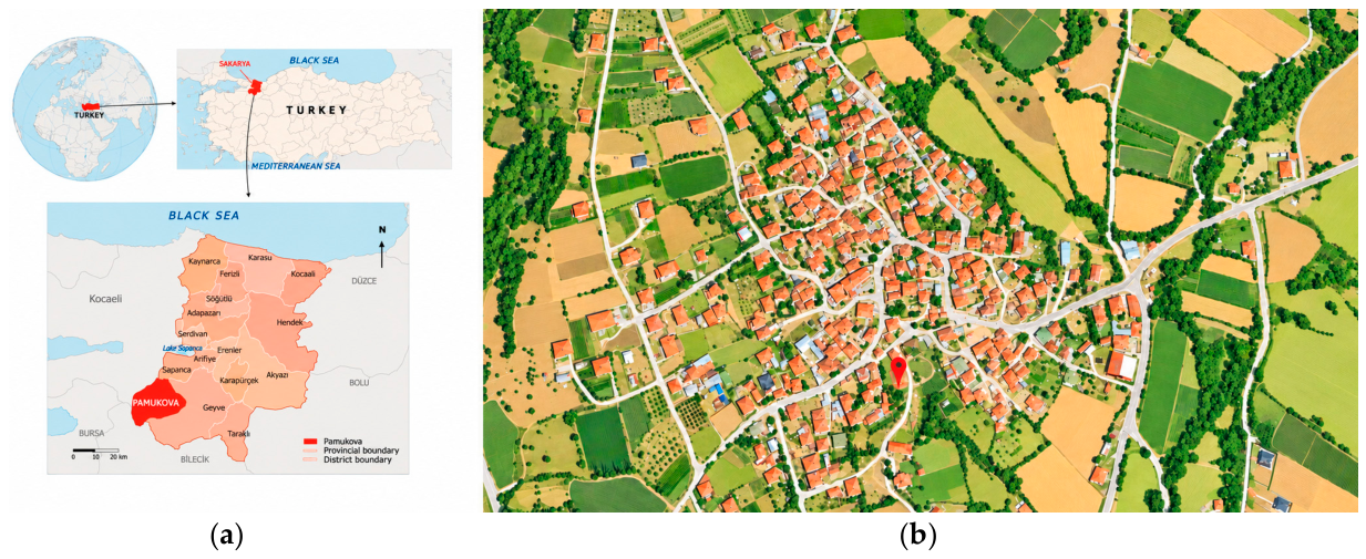
Figure 2.
Dwelling examined in this study: (a) northeast facade; (b) southwest facade; (c) room Z04; (d) room 102 [19].
Figure 2.
Dwelling examined in this study: (a) northeast facade; (b) southwest facade; (c) room Z04; (d) room 102 [19].
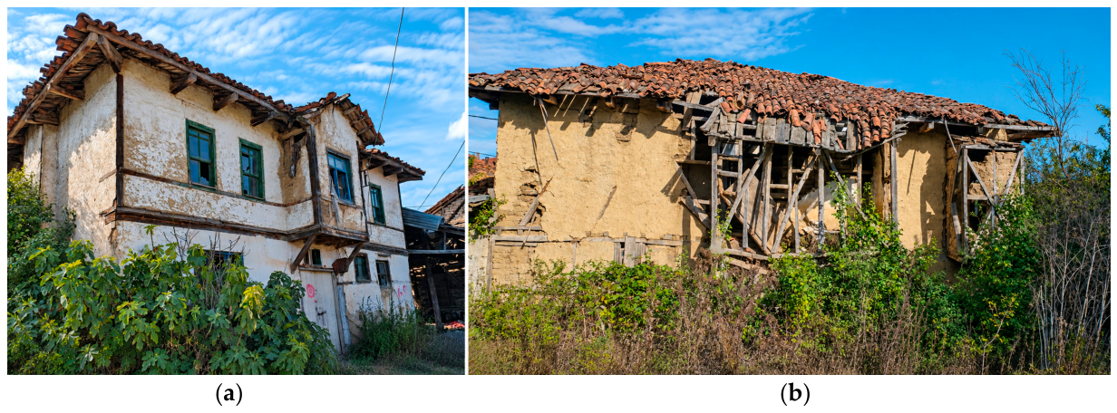
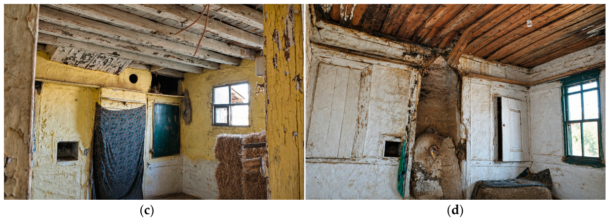
Figure 3.
Plans of the dwelling on cadastral block 209, parcel 17: (a) site plan; (b) ground-floor plan; (c) first-floor plan [20].
Figure 3.
Plans of the dwelling on cadastral block 209, parcel 17: (a) site plan; (b) ground-floor plan; (c) first-floor plan [20].
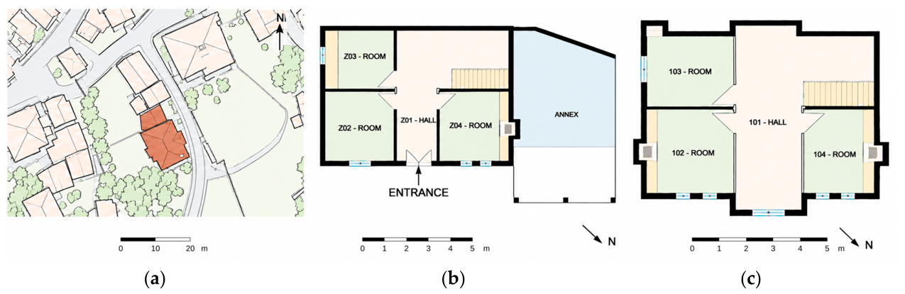
Figure 4.
Thermal zoning scheme and room floor areas in the dwelling’s energy model: (a) ground-floor plan; (b) first-floor plan.
Figure 4.
Thermal zoning scheme and room floor areas in the dwelling’s energy model: (a) ground-floor plan; (b) first-floor plan.
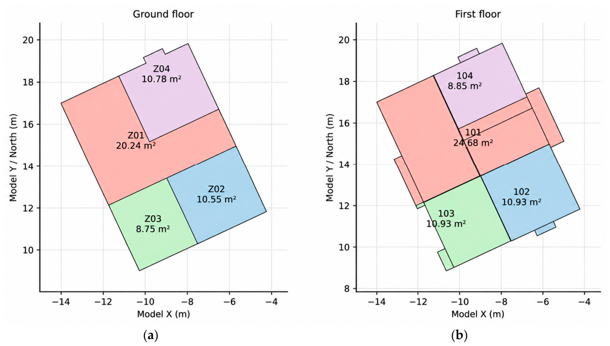
Figure 5.
Three-dimensional model of the dwelling and its immediate surroundings developed in DesignBuilder.
Figure 5.
Three-dimensional model of the dwelling and its immediate surroundings developed in DesignBuilder.
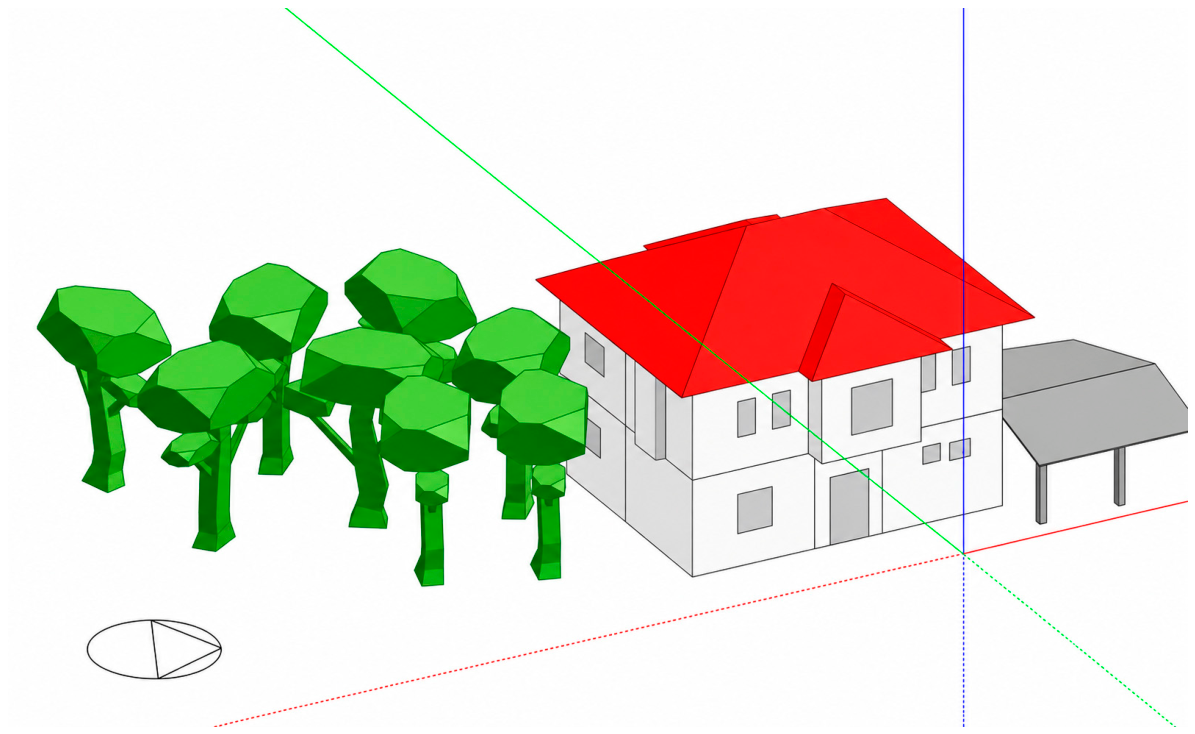
Figure 6.
Climate normals for the Sakarya station and regional climate classification: (a) monthly temperature and precipitation normals for 1991–2020 [25]; (b) location of Sakarya on MGM’s Köppen climate classification map of Türkiye [24]. The data and map were adapted for this study.
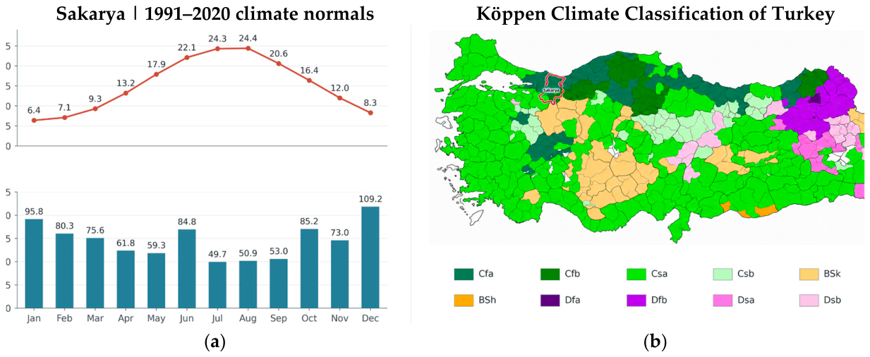
Figure 7.
Hybrid weather file based on 2024 data used in this study: (a) monthly temperatures; (b) summary of solar irradiation.
Figure 7.
Hybrid weather file based on 2024 data used in this study: (a) monthly temperatures; (b) summary of solar irradiation.
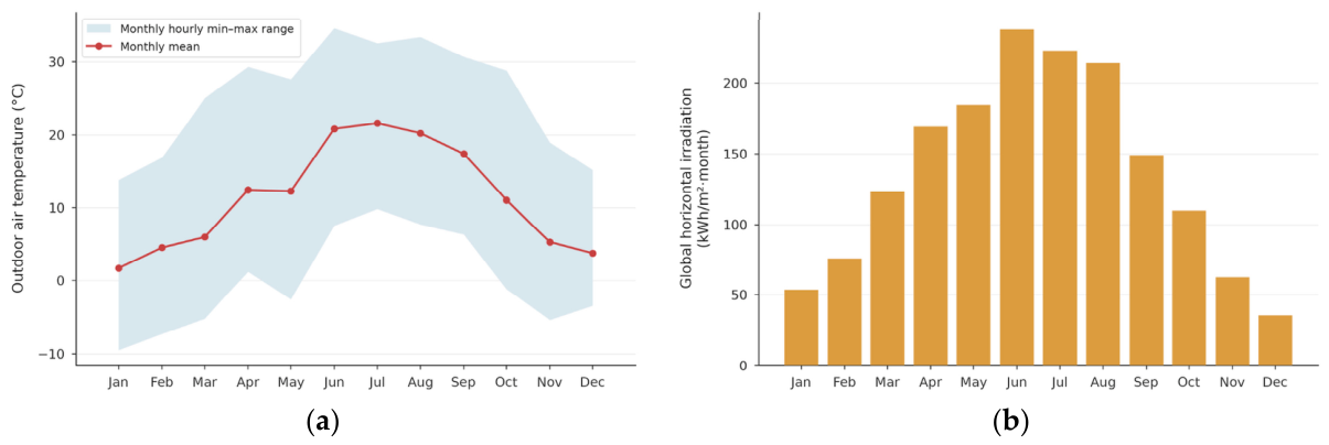
Figure 8.
Room occupancy fraction profiles used in the model: (a) winter day; (b) summer day.
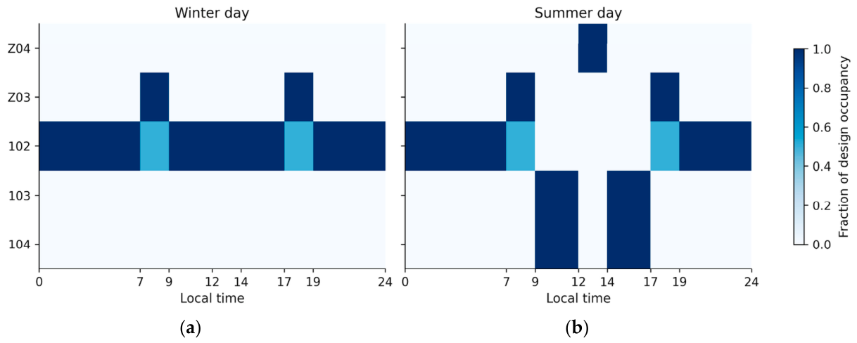
Figure 9.
Changes with ceiling insulation thickness: (a) annual heating demand; (b) nominal thermal transmittance of the ceiling assembly, calculated using a surface resistance of 0.10 m²·K/W on each side for upward heat flow.
Figure 9.
Changes with ceiling insulation thickness: (a) annual heating demand; (b) nominal thermal transmittance of the ceiling assembly, calculated using a surface resistance of 0.10 m²·K/W on each side for upward heat flow.
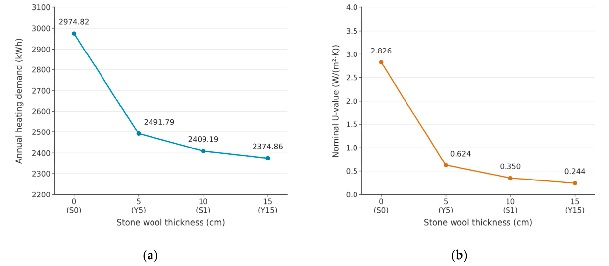
Figure 10.
Breakdown of annual final energy consumption into heating fuel, cooking fuel, and electricity for the eight scenarios. The hatched bar represents S2_1ACH. Values above the bars indicate total consumption rounded to the nearest kWh; results to two decimal places are presented in Table 10.
Figure 10.
Breakdown of annual final energy consumption into heating fuel, cooking fuel, and electricity for the eight scenarios. The hatched bar represents S2_1ACH. Values above the bars indicate total consumption rounded to the nearest kWh; results to two decimal places are presented in Table 10.
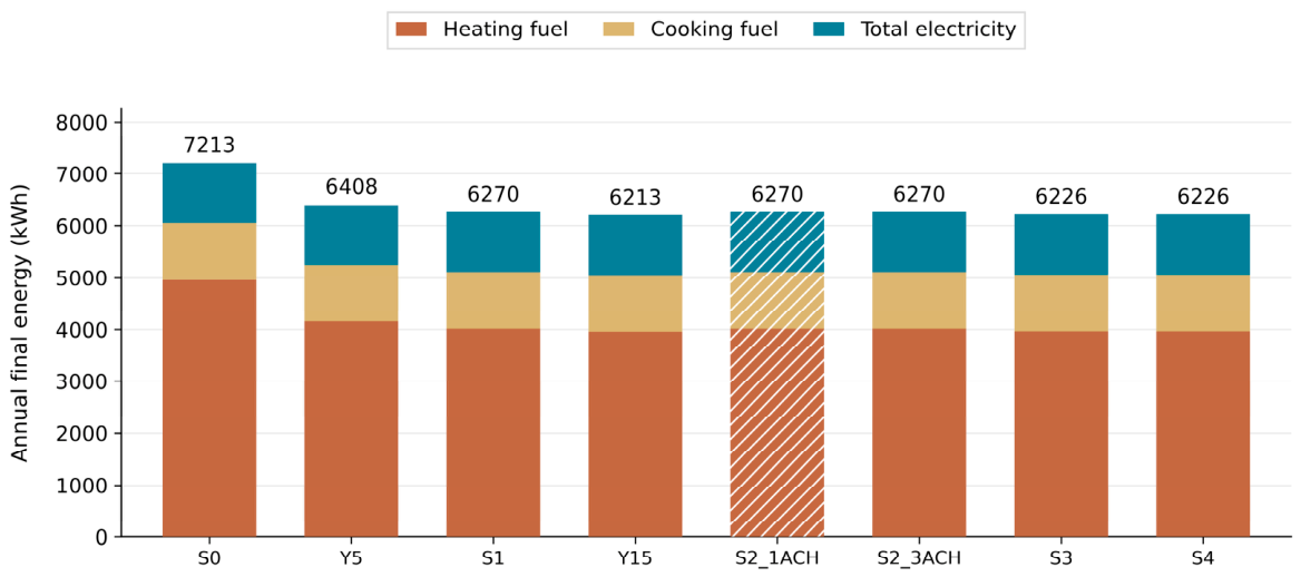
Figure 11.
Summer operative temperature exceedance durations above 28 °C for the eight scenarios: (a) exceedance durations by room (hours); (b) sum of exceedance durations across the eight rooms (room-hours). Each heatmap cell represents the exceedance duration over the same 2928-hour period (1 June–30 September).
Figure 11.
Summer operative temperature exceedance durations above 28 °C for the eight scenarios: (a) exceedance durations by room (hours); (b) sum of exceedance durations across the eight rooms (room-hours). Each heatmap cell represents the exceedance duration over the same 2928-hour period (1 June–30 September).
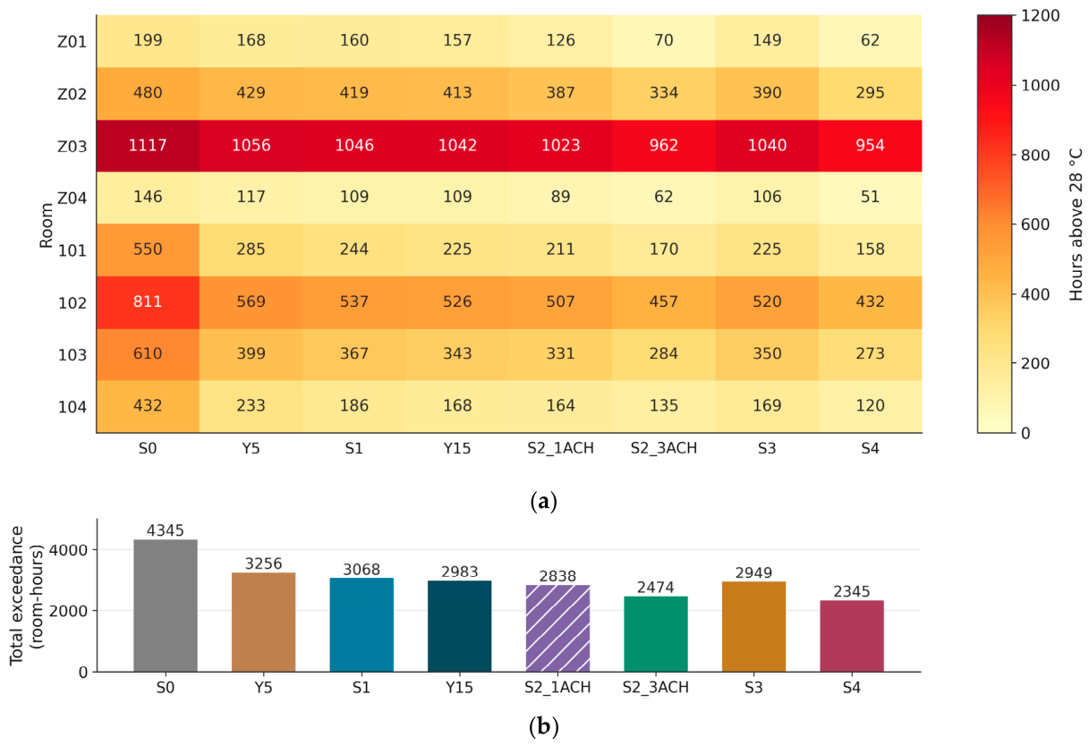
Figure 12.
Summer operative temperature exceedance durations above 28 °C for scenarios S0, S1, S2_1ACH, S2_3ACH, S3, and S4: (a) daytime (07:00–23:00); (b) nighttime (23:00–07:00). Exceedance durations are summed across the eight rooms and expressed in room-hours. The panels use different vertical axis scales.
Figure 12.
Summer operative temperature exceedance durations above 28 °C for scenarios S0, S1, S2_1ACH, S2_3ACH, S3, and S4: (a) daytime (07:00–23:00); (b) nighttime (23:00–07:00). Exceedance durations are summed across the eight rooms and expressed in room-hours. The panels use different vertical axis scales.
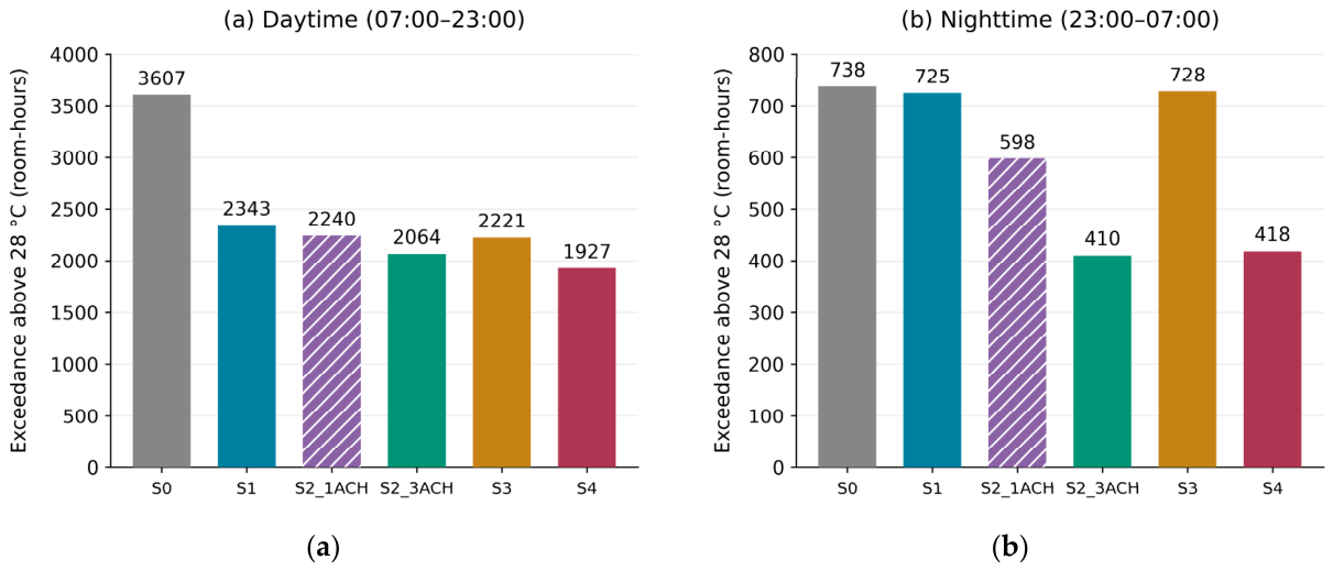
Figure 13.
Occupancy-weighted operative temperature exceedance above 28 °C for scenarios S0, S1, S2_1ACH, S2_3ACH, S3, and S4: (a) total for the summer period (1 June–30 September); (b) nighttime (23:00–07:00). Values are expressed in person-hours. The panels use different vertical axis scales.
Figure 13.
Occupancy-weighted operative temperature exceedance above 28 °C for scenarios S0, S1, S2_1ACH, S2_3ACH, S3, and S4: (a) total for the summer period (1 June–30 September); (b) nighttime (23:00–07:00). Values are expressed in person-hours. The panels use different vertical axis scales.
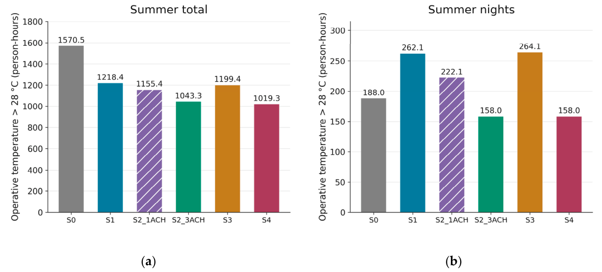
Figure 14.
Variations in temperature and heating power in room 102 during the first week of January: (a) operative temperatures in S0, S1, and S4, indoor air temperature in S4, and outdoor air temperature; (b) heating power in S0, S1, and S4.
Figure 14.
Variations in temperature and heating power in room 102 during the first week of January: (a) operative temperatures in S0, S1, and S4, indoor air temperature in S4, and outdoor air temperature; (b) heating power in S0, S1, and S4.
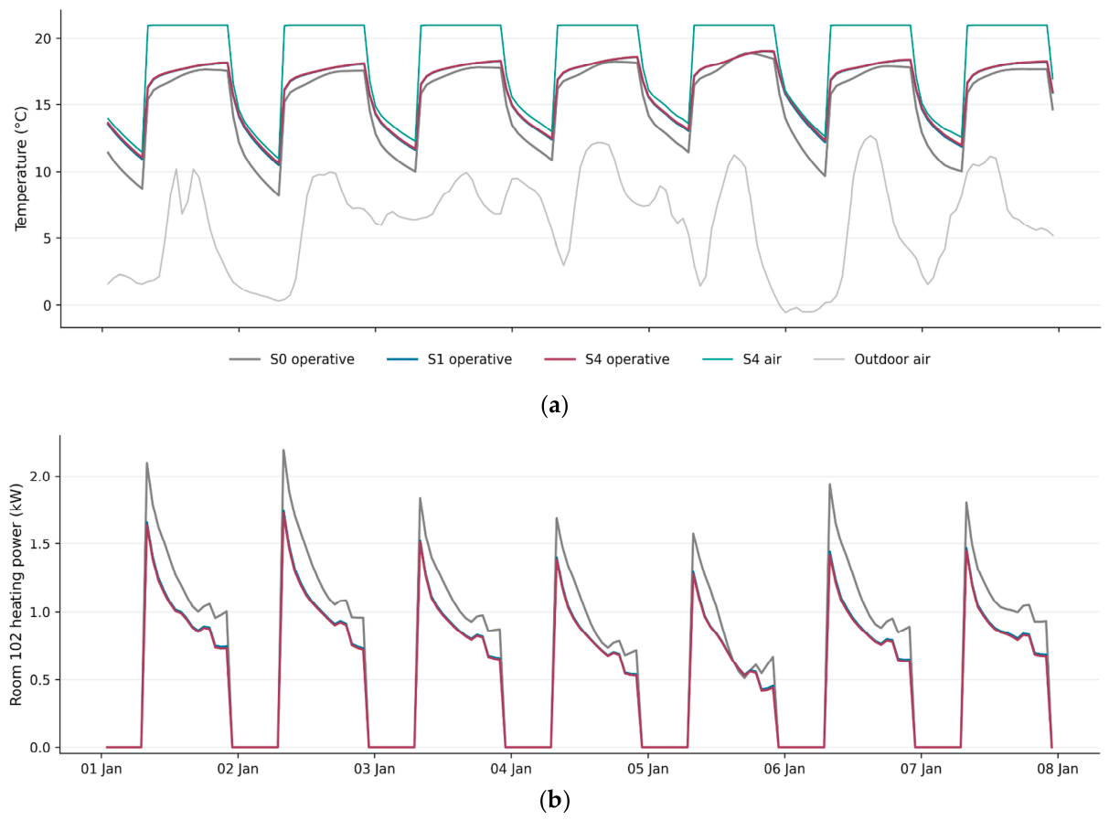
Figure 15.
Hourly operative temperatures for scenarios S1, S2_3ACH, S3, and S4 during 18–22 July: (a) room Z03; (b) room 102. The gray line represents outdoor air temperature, and the horizontal dotted lines indicate the 28 °C threshold. The shared legend between the panels applies to both panels.
Figure 15.
Hourly operative temperatures for scenarios S1, S2_3ACH, S3, and S4 during 18–22 July: (a) room Z03; (b) room 102. The gray line represents outdoor air temperature, and the horizontal dotted lines indicate the 28 °C threshold. The shared legend between the panels applies to both panels.
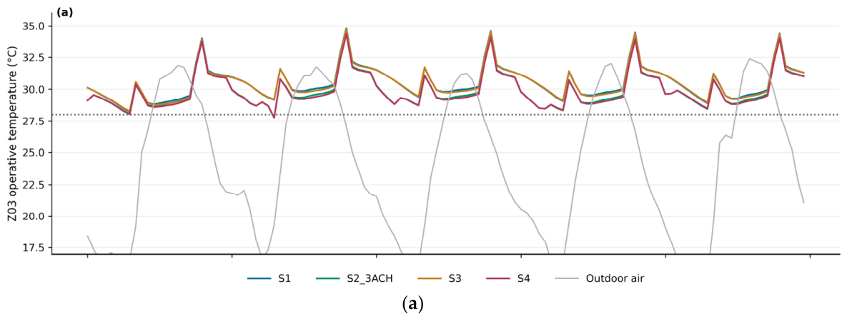
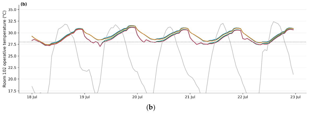
Figure 16.
Comparison of annual heating demand and operative temperature exceedance durations above 28 °C across the eight scenarios: (a) total for the summer period; (b) nighttime hours during summer (23:00–07:00). Exceedance durations are summed across the eight rooms and expressed in room-hours. The purple diamond represents S2_1ACH, in which the nominal air change rate is set to 1 h⁻¹. The panels use different vertical axis scales.
Figure 16.
Comparison of annual heating demand and operative temperature exceedance durations above 28 °C across the eight scenarios: (a) total for the summer period; (b) nighttime hours during summer (23:00–07:00). Exceedance durations are summed across the eight rooms and expressed in room-hours. The purple diamond represents S2_1ACH, in which the nominal air change rate is set to 1 h⁻¹. The panels use different vertical axis scales.
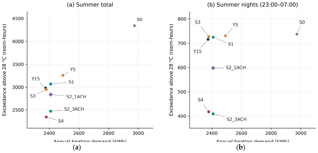

Table 1.
Comparison of approaches adopted in selected studies with the scope of the Kemaliye study.
| Assessment dimension | Approaches adopted in selected studies | Scope of the Kemaliye study |
| Building and climatic context | Timur et al. [11] examined traditional dwellings in Muğla; Dervishi et al. [12] investigated traditional dwelling typologies in Albania; and Lozoya-Peral et al. [4] studied a traditional building in the dry Mediterranean climate of southeastern Spain. | The study examined a traditional rural dwelling with a timber frame and infill walls in Kemaliye village, Pamukova district, Sakarya province. The findings are specific to the building’s physical characteristics, local climate data, and defined patterns of use. |
| Research methods and data sources | Timur et al. [11] combined field measurements, material testing, and DesignBuilder simulations. Lozoya-Peral et al. [4] compared different energy retrofit interventions through simulation. | The dwelling was modeled in its existing condition using DesignBuilder, and the baseline and retrofit scenarios were compared under identical boundary conditions. The model was not calibrated against field measurements. |
| Energy performance | Dervishi et al. [12] examined the effects of building envelope retrofit scenarios on energy performance, while Lozoya-Peral et al. [4] investigated the effects of changes in insulation and window properties on energy demand. | Annual heating demand and final energy consumption were assessed as separate indicators, and their percentage changes relative to the corresponding reference scenario were compared. |
| Summer thermal conditions | Lozoya-Peral et al. [4] showed that insulation could reduce heating demand while prolonging periods of elevated indoor temperatures in summer, whereas natural ventilation could limit overheating. | Hourly operative temperatures during summer, durations of temperature exceedance above 28 °C, and overheating indicators were assessed at the room level. The relationship between energy savings and summer thermal conditions was examined. |
| Thermal comfort approach | Brager and de Dear [9] examined the relationship between thermal comfort, environmental conditions, and occupant adaptation. de Dear et al. [10] reviewed approaches and developments in adaptive thermal comfort research. | Summer thermal conditions were assessed using exceedance indicators based on a specified temperature threshold. These indicators were not interpreted as measures of occupant satisfaction validated against an adaptive thermal comfort standard. |
| Partial heating and patterns of use | Karabeyeser Bakan et al. [3] used interviews to examine the relationships between occupants’ thermal comfort perceptions and decisions concerning energy efficiency and conservation in historic dwellings. In her study of Osmaneli, Ergöz Karahan [5] noted that space use during the winter months could be concentrated in one or two rooms in stove-heated dwellings. Shetty and Patil [8] assessed factors influencing occupants’ spatial experiences and satisfaction with the indoor environment. | The modeled pattern of use involved heating only one designated room of the dwelling. Thermal conditions in heated and unheated rooms were assessed in accordance with the defined heating and occupancy schedules. |
| Room-level and temporal scales | Timur et al. [11] examined the energy and thermal performance of traditional dwellings using measurement and simulation data. Lozoya-Peral et al. [4] compared the effects of energy retrofit interventions on energy demand and indoor temperatures. | Annual heating energy was assessed at the building level, while summer operative temperatures and overheating indicators were evaluated on an hourly basis for each room. Temperature exceedance durations were also examined in relation to occupancy hours. |
| Energy retrofit strategies | Timur et al. [11] examined interventions such as floor insulation, airtightness improvements, and secondary glazing; Dervishi et al. [12] investigated improvements to wall, roof, and window properties; and Lozoya-Peral et al. [4] considered insulation, glazing properties, window dimensions, and natural ventilation strategies. | Ceiling insulation thicknesses of 5, 10, and 15 cm were compared. Relative to a common baseline with 10 cm of insulation, the additional effects of secondary glazing, controlled night ventilation at air change rates of 1 and 3 h⁻¹, and the combination of secondary glazing with night ventilation at 3 h⁻¹ were evaluated. |
| Architectural conservation and intervention compatibility | Fiore et al. [7] examined the relationship between energy efficiency and conservation requirements in historic buildings, emphasizing the technical and aesthetic suitability of interventions, material compatibility, and reversibility. Karabeyeser Bakan et al. [3] assessed the role of heritage values in energy retrofit decisions. | The interventions were discussed in the context of preserving the traditional construction system and original architectural features. As moisture behavior and long-term material durability were not analyzed, the suitability of the interventions from a conservation perspective was not conclusively established. |
| Relationship between occupant satisfaction and the indoor environment | Shetty and Patil [8] examined the relationships between spatial organization, natural ventilation, local materials, sociocultural conditions, and satisfaction with the indoor environment in vernacular architecture. Karabeyeser Bakan et al. [3] assessed the influence of occupants’ comfort perceptions on energy and conservation decisions. | Occupant behavior was represented by the heating and room occupancy schedules defined in the simulation. Occupancy-weighted temperature exceedance indicators were assessed; occupant satisfaction was not measured through surveys or interviews. |
| Model reliability and limitations | Timur et al. [11] integrated field measurements and material test results with simulations. Lozoya-Peral et al. [4] and Dervishi et al. [12] evaluated energy retrofit options under specified modeling and climatic conditions. | The results are based on meteorological data, material properties, and operational assumptions. As the model was not calibrated against measured data, the findings were interpreted in terms of relative performance changes across scenarios. |
| Distinctive approach of the study | Timur et al. [11], Dervishi et al. [12], and Lozoya-Peral et al. [4] examined the effects of energy retrofit interventions on the energy and thermal performance of traditional dwellings. Karabeyeser Bakan et al. [3] and Shetty and Patil [8] addressed variables related to occupant perceptions, patterns of space use, and satisfaction with the indoor environment. | For a partially heated traditional rural dwelling, the effects of the same retrofit scenarios were compared in terms of both annual heating energy demand and room-level summer overheating indicators linked to occupancy hours. |
* This table compares methodological approaches in selected studies with the scope of the Kemaliye study; it does not constitute a systematic literature review. Numerical results obtained under different climatic conditions, building characteristics, and patterns of use were not directly compared. The temperature exceedance indicators used in the Kemaliye study were not interpreted as measures of occupant satisfaction or as thermal comfort levels verified against standards.
Table 2.
Room floor areas and volumes in the DesignBuilder model.
| Room | Function | Floor area (m²) | Volume (m³) | Active heating |
| Z01 | Hall | 20.2445 | 54.6602 | No |
| Z02 | Storage | 10.5544 | 28.4969 | No |
| Z03 | Kitchen/storage | 8.7532 | 23.6336 | No |
| Z04 | Traditional room | 10.7818 | 29.1109 | No |
| 101 | Hall | 24.6770 | 65.8877 | No |
| 102 | Traditional room | 10.9317 | 29.1875 | Yes |
| 103 | Traditional room | 10.9303 | 23.9258 | No |
| 104 | Traditional room | 8.8531 | 23.6378 | No |
Table 3.
Thermophysical properties and IDF record names of the materials defined in the model.
| Material |
λ [W/(m·K)] Thermal conductivity |
ρ [kg/m³] Density |
cₚ [J/(kg·K)] Specific heat capacity |
IDF record name |
| Timber | 0.13 | 500 | 1600 | Project-specific record: kemaliye_ahsap |
| Lime plaster | 0.80 | 1600 | 1000 | Project-specific record: kemaliye_kirec_siva |
| Equivalent timber–adobe layer | 0.36 | 1140 | 1040 | Project-specific equivalent record: kemaliye_karkas_kerpic_esdeger |
| Limestone rubble masonry (dry) | 1.40 | 2200 | 840 | Masonry - quarrystones, calcareous Dry |
| Painted oak | 0.19 | 700 | 2390 | Painted Oak |
| Stone wool (rolls) | 0.04 | 30 | 840 | MW Stone Wool (rolls) |
| Clay roof tiles | 1.00 | 2000 | 800 | Clay Tile (roofing) |
Table 4.
Building components and layer thicknesses.
| Component | Layers (outside to inside) | Total thickness |
| External wall | 2 cm lime plaster + 16 cm equivalent timber–adobe layer + 2 cm lime plaster | 20 cm |
| Internal partition | 2 cm lime plaster + 12 cm equivalent timber–adobe layer + 2 cm lime plaster | 16 cm |
| Baseline ceiling | Timber | 2 cm |
| Scenarios with 10 cm insulation S1, S2_1ACH, S2_3ACH, S3, S4 |
10 cm stone wool + 2 cm timber | 12 cm |
| Pitched roof | 2 cm clay tiles + 2.5 cm timber | 4.5 cm |
| Ground and intermediate floors | Timber | 3 cm |
| Foundation wall | Limestone (dry) | 50 cm |
| External / internal door | Painted oak | 4 / 3.5 cm |
Table 5.
Summary indicators calculated from Sakarya’s 1991–2020 climate normals.
| Indicator | Value | Period / scope |
| Mean temperature of the coldest month | 6.4 °C | January |
| Mean temperature of the warmest month | 24.4 °C | August |
| Arithmetic mean of monthly mean temperatures | 15.17 °C | January–December |
| Mean annual total precipitation | 878.6 mm | January–December |
| Total precipitation in the summer half-year | 359.5 mm | April–September; 40.9% of annual precipitation |
| Total precipitation in the winter half-year | 519.1 mm | October–March; 59.1% of annual precipitation |
| Precipitation in the driest month of the summer half-year | 49.7 mm | July |
| Precipitation in the wettest month of the winter half-year | 109.2 mm | December |
| Köppen climate class | Cfa | Sakarya meteorological station |
Table 6.
Data sources and extent of gap filling for meteorological variables in the hybrid weather file.
Table 6.
Data sources and extent of gap filling for meteorological variables in the hybrid weather file.
| Variable | Direct source | Regression | Interpolation | Test RMSE |
| Temperature | 7547 h (Kemaliye) | 1194 h | 19 h | 1.923 °C |
| Relative humidity | 7546 h (Kemaliye) | 1195 h | 19 h | 7.202 percentage points |
| Wind | 8752 h (Pamukova) | None | 8 h | Not evaluated |
Table 7.
Numerical simulation settings and boundary conditions.
| Parameter | Value used in the model |
| Simulation period | 1 January–31 December; 8760 h |
| Zone heat balance timestep | 10 min; six timesteps per hour |
| Output reporting interval | Hourly |
| Heat conduction in building elements not modeled with Kiva | Conduction Transfer Function (CTF) |
| Interior surface convection algorithm | TARP |
| Exterior surface convection algorithm | DOE-2 |
| Solar distribution option | FullExterior |
| Terrain class | Suburbs |
| Ground heat transfer model | Kiva |
Table 8.
Operational assumptions held constant across scenarios.
| Parameter | Value used in the model |
| Active heating | Room 102 only; October–May, 07:00–22:00 |
| Heating setpoint and representation | 21 °C air temperature; ideal heating load |
| Seasonal heating efficiency | 0.60 |
| Active cooling / domestic hot water | Disabled / disabled |
| Air infiltration | Living spaces: 0.7 h⁻¹; attic: 1.0 h⁻¹; continuous |
| Daylight-responsive lighting control | 50 lux; continuous dimming; minimum power and light output fractions of 0.10 |
Table 9.
Retrofit components and scope of comparison for the eight scenarios.
| Code | Stone wool | Glazing configuration | Controlled night ventilation | Scope of comparison |
| S0 | None | 4 mm single glazing | Disabled | Existing condition reference |
| Y5 | 5 cm | 4 mm single glazing | Disabled | Effect of insulation thickness (5 cm) |
| S1 | 10 cm | 4 mm single glazing | Disabled | Effect of insulation thickness; common reference for subsequent interventions |
| Y15 | 15 cm | 4 mm single glazing | Disabled | Effect of insulation thickness (15 cm) |
| S2_1ACH | 10 cm | 4 mm single glazing | 1 h⁻¹ (controlled) | Additional effect of ventilation relative to S1; comparison of ventilation rates with S2_3ACH |
| S2_3ACH | 10 cm | 4 mm single glazing | 3 h⁻¹ (controlled) | Additional effect of night ventilation relative to S1 |
| S3 | 10 cm | 4–50 (air gap)–4 mm | Disabled | Additional effect of secondary glazing relative to S1 |
| S4 | 10 cm | 4–50 (air gap)–4 mm | 3 h⁻¹ (controlled) | Comparison of the combined intervention with S2_3ACH and S3 |
Table 10.
Annual energy results for the scenarios.
| Scenario |
Heating demand (kWh) |
Heating fuel energy (kWh) |
Electricity consumption (kWh) |
Final energy consumption (kWh) |
| S0 | 2974.82 | 4958.03 | 1159.51 | 7212.93 |
| Y5 | 2491.79 | 4152.98 | 1159.51 | 6407.87 |
| S1 | 2409.19 | 4015.32 | 1159.51 | 6270.22 |
| Y15 | 2374.86 | 3958.10 | 1159.51 | 6213.00 |
| S2_1ACH | 2409.20 | 4015.33 | 1159.51 | 6270.23 |
| S2_3ACH | 2409.21 | 4015.35 | 1159.51 | 6270.25 |
| S3 | 2379.18 | 3965.30 | 1165.45 | 6226.14 |
| S4 | 2379.20 | 3965.33 | 1165.45 | 6226.18 |
Note: Cooking fuel energy consumption is 1095.39 kWh in all scenarios. Electricity consumption includes appliances and interior and exterior lighting. Heating energy delivered to the room was not added separately to the final energy total. Totals were calculated from unrounded output values; therefore, minor rounding differences may occur between the reported totals and the sums of the displayed components.
Table 11.
Summer operative temperature exceedance indicators for scenarios S0, S1, S2_1ACH, S2_3ACH, S3, and S4.
Table 11.
Summer operative temperature exceedance indicators for scenarios S0, S1, S2_1ACH, S2_3ACH, S3, and S4.
| Scenario |
Exceedance duration above 26 °C (room-hours) |
Exceedance duration above 28 °C (room-hours) |
Exceedance duration above 30 °C (room-hours) |
Degree-hours above 28 °C (K·room-hours) |
| S0 | 10,719 | 4345 | 1161 | 6280.58 |
| S1 | 9570 | 3068 | 498 | 3475.84 |
| S2_1ACH | 9382 | 2838 | 414 | 3094.73 |
| S2_3ACH | 9064 | 2474 | 325 | 2598.85 |
| S3 | 9361 | 2949 | 461 | 3304.91 |
| S4 | 8848 | 2345 | 307 | 2438.22 |
Note: The values represent the sum of the results for the eight rooms over the same 2928-hour period. Degree-hours account for both the duration of exceedance and the extent to which the temperature exceeds the threshold.
Table 12.
Summer operative temperatures and exceedance durations by room in scenario S4.
| Room |
Mean operative temperature (°C) |
Maximum operative temperature (°C) |
Exceedance duration above 28 °C (hours) |
Nighttime exceedance duration above 28 °C (hours) |
| Z01 | 24.71 | 29.02 | 62 | 2 |
| Z02 | 25.67 | 30.07 | 295 | 37 |
| Z03 | 27.09 | 34.35 | 954 | 223 |
| Z04 | 24.31 | 28.71 | 51 | 0 |
| 101 | 24.51 | 30.40 | 158 | 10 |
| 102 | 25.75 | 31.93 | 432 | 79 |
| 103 | 25.30 | 30.89 | 273 | 56 |
| 104 | 24.22 | 30.05 | 120 | 11 |
Note: The summer period is defined as 1 June–30 September, and the nighttime period as 23:00–07:00. Nighttime exceedance durations are included in the total exceedance duration reported in the same row.
Table 13.
Summer operative temperature exceedance above 28 °C weighted by the occupancy schedule.
| Scenario |
Summer exceedance duration (person-hours) |
Nighttime exceedance duration (person-hours) |
Summer degree-hours (person·K·h) |
| S0 | 1570.46 | 188.05 | 2761.88 |
| S1 | 1218.37 | 262.07 | 1770.12 |
| S2_1ACH | 1155.36 | 222.06 | 1640.39 |
| S2_3ACH | 1043.33 | 158.04 | 1466.05 |
| S3 | 1199.37 | 264.07 | 1721.37 |
| S4 | 1019.33 | 158.04 | 1415.10 |
Note: The summer period covers 1 June–30 September, and nighttime is defined as 23:00–07:00. The occupancy-weighted degree-hour indicator accounts for both the hourly number of occupants and the temperature difference above the threshold.
Table 14.
Mean temperatures and durations of low operative temperature in room 102 during winter heating hours.
Table 14.
Mean temperatures and durations of low operative temperature in room 102 during winter heating hours.
| Scenario |
Mean air temperature (°C) |
Mean radiant temperature (°C) |
Mean operative temperature (°C) |
Duration with operative temperature below 18 °C (hours) |
| S0 | 21.00 | 13.08 | 17.04 | 1146 |
| Y5 | 21.00 | 13.98 | 17.49 | 1026 |
| S1 | 21.00 | 14.14 | 17.57 | 975 |
| Y15 | 21.00 | 14.21 | 17.60 | 954 |
| S2_1ACH | 21.00 | 14.14 | 17.57 | 975 |
| S2_3ACH | 21.00 | 14.14 | 17.57 | 975 |
| S3 | 21.00 | 14.20 | 17.60 | 957 |
| S4 | 21.00 | 14.20 | 17.60 | 957 |
Note: All values refer to the same assessment period, comprising 1350 h between 07:00 and 22:00 during December, January, and February.
Disclaimer/Publisher’s Note: The statements, opinions and data contained in all publications are solely those of the individual author(s) and contributor(s) and not of MDPI and/or the editor(s). MDPI and/or the editor(s) disclaim responsibility for any injury to people or property resulting from any ideas, methods, instructions or products referred to in the content. |
© 2026 by the authors. Licensee MDPI, Basel, Switzerland. This article is an open access article distributed under the terms and conditions of the Creative Commons Attribution (CC BY) license (http://creativecommons.org/licenses/by/4.0/).
Copyright: This open access article is published under a Creative Commons CC BY 4.0 license, which permit the free download, distribution, and reuse, provided that the author and preprint are cited in any reuse.